Low-level atmospheric turbulence dataset in China generated by combining radar wind profiler and radiosonde observations

Low-level atmospheric turbulence plays a critical role in cloud dynamics and aviation safety. Nevertheless, altitude-resolved turbulence profiles remain scarce, largely owing to observational challenges. By leveraging collocated radar wind profiler (RWP) and radiosonde observations from 29 stations across China in 2023, a high vertical resolution dataset of low-level turbulence-related parameters is generated based on the spectral width method. This dataset includes squared Brunt–Väisälä frequency (N²), turbulent dissipation rate (ε), vertical eddy diffusivity (K), inner scale (l₀), and buoyancy length scale (L_B), which are provided twice daily at 00:00 and 12:00 UTC with a vertical resolution of 120 m, covering altitudes from 0.12 to 3.0 km above ground level (a.g.l.). Spatial analysis reveals significant regional disparities in turbulence-related parameters across China, where ε, K, and L_B are higher in northwest and north China compared to south China, while N² and l₀ display an inverse spatial pattern. These contrasting geographical distributions suggest distinct atmospheric instability across China. In terms of seasonality, turbulence-related variables showed maxima during spring and summer. Vertical profile characteristics show distinct altitudinal dependencies: ε, L_B, and K exhibit progressive attenuation with altitude, while N² and l₀ increase with altitude. Statistical analysis indicates that ε and K follow log-normal distributions, whereas l₀ and L_B align with Gamma distributions. This dataset is publicly accessible at https://doi.org/10.5281/zenodo.14959025 (Meng and Guo, 2025) and provides crucial insights into the fine-scale structural evolution of low-level turbulence. The preliminary findings based on the dataset have great implications for improving our understanding of the pre-storm environment, conducting scientific planning, and guiding low-level flight routes in the emerging low-altitude economy in China.

1 Introduction

The low-level atmosphere below 3.0 km altitude serves as a critical interface for planetary boundary layer (PBL) and cloud interactions and for convective initiation processes (Marquis et al., 2021; Nowak et al., 2021). This dynamic transition zone facilitates exchange of water vapor, thermal energy, moment flux, and aerosol particles between Earth's surface and free atmosphere (Muñoz-Esparza et al., 2018; Brunke et al., 2022). The turbulence-driven exchanges can be quantitatively characterized by key physical parameters such as N², ε, K, l₀, L_B, and atmospheric refractive index structure constant (Cn²) (Fukao et al., 1994; Wilson, 2004). These parameters collectively govern the energy cascade processes and momentum transfer mechanisms that dominate PBL thermodynamics. Accurately understanding the spatiotemporal evolution of low-level turbulence is crucial not only for improving the predictive skill of severe convective systems through refined parameterization schemes but also for implementing operational safeguards for low-altitude aviation safety.

Therefore, advances have been made in recent years in observational techniques for characterizing low-level turbulence. Conventional in-situ platforms include weather balloons (e.g., Clayson and Kantha, 2008; Guo et al., 2016; Kohma et al., 2019), rockets (Namboodiri et al., 2011), and aircraft (Nicholls et al., 1984; Brunke et al., 2022; Chechin et al., 2023). Concurrently, unoccupied aerial vehicles (UAVs) have demonstrated growing potential in capturing low-level turbulence features that traditional aircraft and radiosonde networks cannot systematically resolve (Shelekhov et al., 2021). Nevertheless, these approaches face inherent limitations, such as high operational costs, discontinuous temporal sampling, and spatially constrained coverage limited to point measurements or linear transects. Such restrictions fundamentally impede the acquisition of vertically resolved turbulence profiles with sufficient spatiotemporal continuity.

To address these observational gaps, ground-based lidars and radars have emerged as pivotal solutions (Gage and Balsley, 1978). Radar wind profilers (RWPs) and coherent Doppler wind lidar systems have demonstrated effectiveness in obtaining turbulence parameters with both high temporal resolution and operational continuity (Sato and Woodman, 1982; Hocking, 1985; Fukao et al., 1994; Nastrom and Eaton, 1997; Luce et al., 2023a; Meng et al., 2024).

ε, in conjunction with K, l₀, and L_B, derivable from ε (Fukao et al., 1994), serves as a critical determinant in radar-derived quantification of atmospheric turbulence metrics. Three principal methodological frameworks have emerged for retrieving ε in the low-level atmosphere from RWP observations, namely the power method (Hocking, 1985; Hocking and Mu, 1997), variance method (Satheesan and Murthy, 2002), and Doppler spectral width method (Nastrom, 1997; Dehghan and Hocking, 2011). The power method utilizes backscattered signal intensity modulated by refractive index fluctuations (Weinstock, 1981a; Cohn, 1995). The variance method establishes a direct mathematical relationship between ε and the variance of vertical velocity (Satheesan and Murthy, 2002). Comprehensive reviews by Cohn (1995), Gage and Balsley (1978), and Wilson (2004) have thoroughly evaluated their underlying assumptions, advantages, and limitations. As highlighted by Satheesan and Murthy (2002), the power method necessitates thermodynamic profiles, and the variance method demands accuracy in Doppler measurements, particularly challenged by contamination from non-turbulent motions in vertical beam observations, while the influence of ground clutter and the differences in the calculation of various spectral broadening terms are the main factors contributing to the large uncertainty in turbulence spectral width. Most widely adopted is the Doppler spectrum width technique, which isolates turbulence-induced spectral broadening through systematic removal of non-turbulent contributions (e.g., Cohn, 1995; Nastrom and Eaton, 1997; Eaton and Nastrom, 1998; Jacoby-Koaly et al., 2002; Dehghan and Hocking, 2011; Kohma et al., 2019; Jaiswal et al., 2020; Solanki et al., 2022; Chen et al., 2022a, b; Luce et al., 2023b). The non-turbulent spectral widths are mainly contributed by beam broadening, shear effects, and gravity wave perturbations, which can be estimated using the algorithms proposed by Hocking (1985), Nastrom (1997), and Dehghan and Hocking (2011), respectively. Recent work by Chen et al. (2022b) identifies a critical vertical wind shear (VWS) threshold of 0.006 s⁻¹, beyond which turbulence spectral width retrievals become increasingly susceptible to negative value artifacts, highlighting unresolved challenges under extreme shear conditions that frequently accompany severe convective systems.

Complementing radar-based methodologies, radiosonde measurements have long been used to derive the profiles of N² and ε using the Thorpe analysis method (Thorpe, 1977). Originally designed to diagnose turbulent overturning in the troposphere and lower stratosphere, this method enables cross-validation with radar-derived turbulence metrics through coordinated multi-platform campaigns (Clayson and Kantha, 2008; Wilson et al., 2014; Li et al., 2016; Kohma et al., 2019; Jaiswal et al., 2020; Lv et al., 2021; Rajput et al., 2022; Ko et al., 2024). Nevertheless, the Thorpe analysis method is not suitable for turbulence retrieval in the low-level atmosphere below 3.0 km a.g.l.

Even though significant strides have been made in calculating temporally continuous profiles of ε, other turbulence-related parameters such as l₀, L_B, and K in the low atmosphere remain insufficiently analyzed, particularly on a national scale, largely due to the lack of concurrent observations of high vertical resolution temperature, humidity, and wind profiles. Fortunately, the RWP observational network has been built up and operated by the China Meteorological Administration (CMA), and most RWP stations are collocated with radiosonde stations. Furthermore, attempts were made to retrieve all the above-mentioned turbulence metrics by combining the measurements of RWP and radiosonde by Solanki et al. (2022). This motivates us to construct such a low-level turbulence dataset in China, enabling a holistic view of the turbulence features throughout China. The paper is structured as follows. Section 2 details the data sources and methodology, including instrumentation specifications from the observational station and the retrieval method employed for turbulence-related parameters. Section 3 presents a multi-scale analysis of turbulence dynamics, encompassing vertical profile examinations and spatiotemporal variation patterns of low-level turbulence in China. Finally, summary and concluding remarks are given in Sect. 4.

2 Data and methodology

2.1 RWP and radiosonde measurements

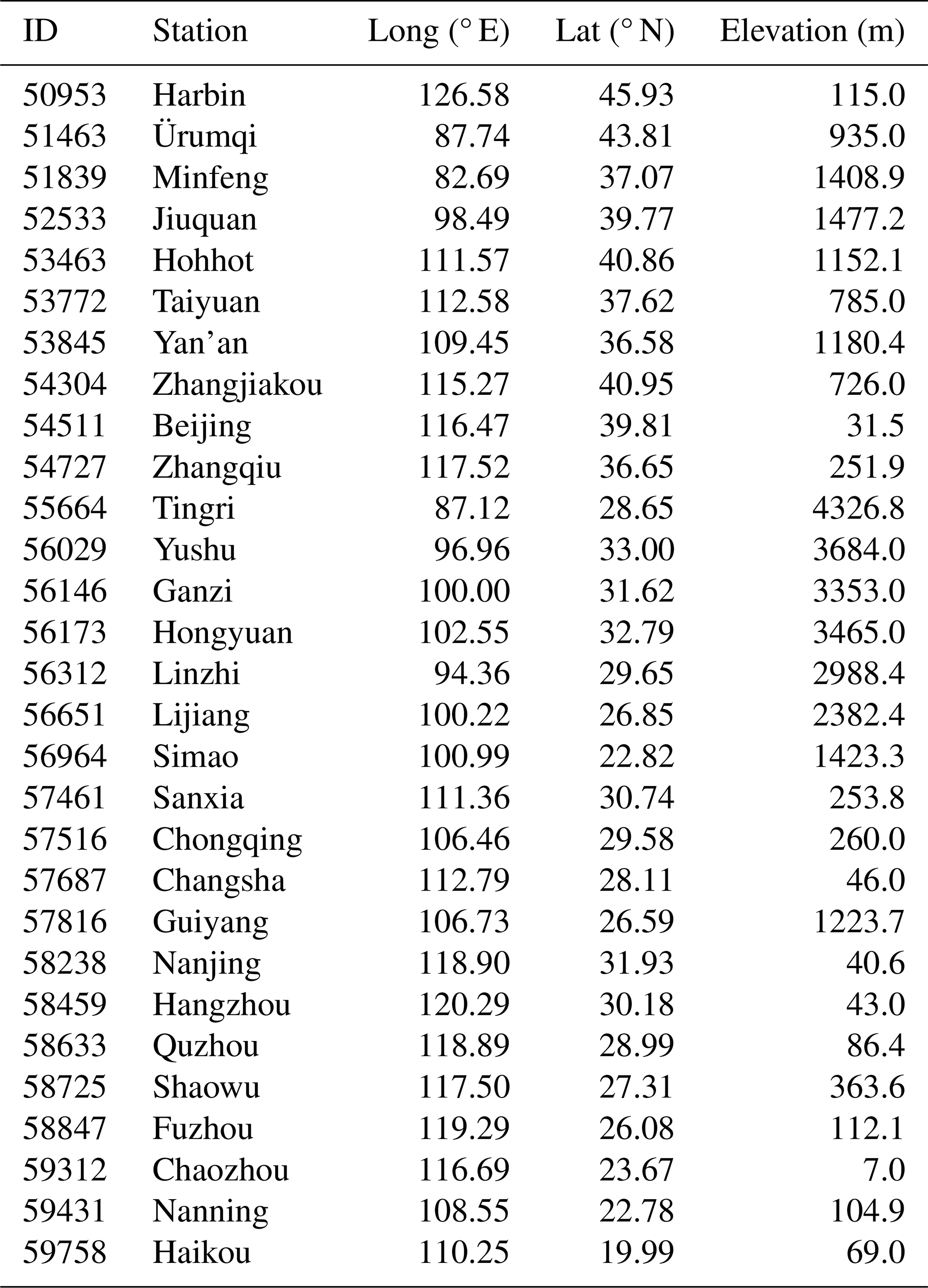
As of 31 December 2023, CMA operates a modern vertical meteorological observing network consisting of 120 L-band radiosonde and over 200 RWP stations. Through a rigorous station selection process, 29 optimally collocated observation stations were identified (Fig. 1) based on systematic evaluation of spatial representativeness and instrument performance metrics. These stations are equipped with an advanced RWP–radiosonde synergetic observation system specifically designed for retrieving low-level turbulence-related parameters. The network spans latitudes from 16.83 to 49.22° N and longitudes from 75.98 to 129.47° E, covering China's primary geomorphological regions, ranging from coastal plains (−0.4 m a.s.l., a.m.s.l.) to high-mountain plateaus (4326.8 m a.m.s.l.). Detailed station information is provided in Table 1.

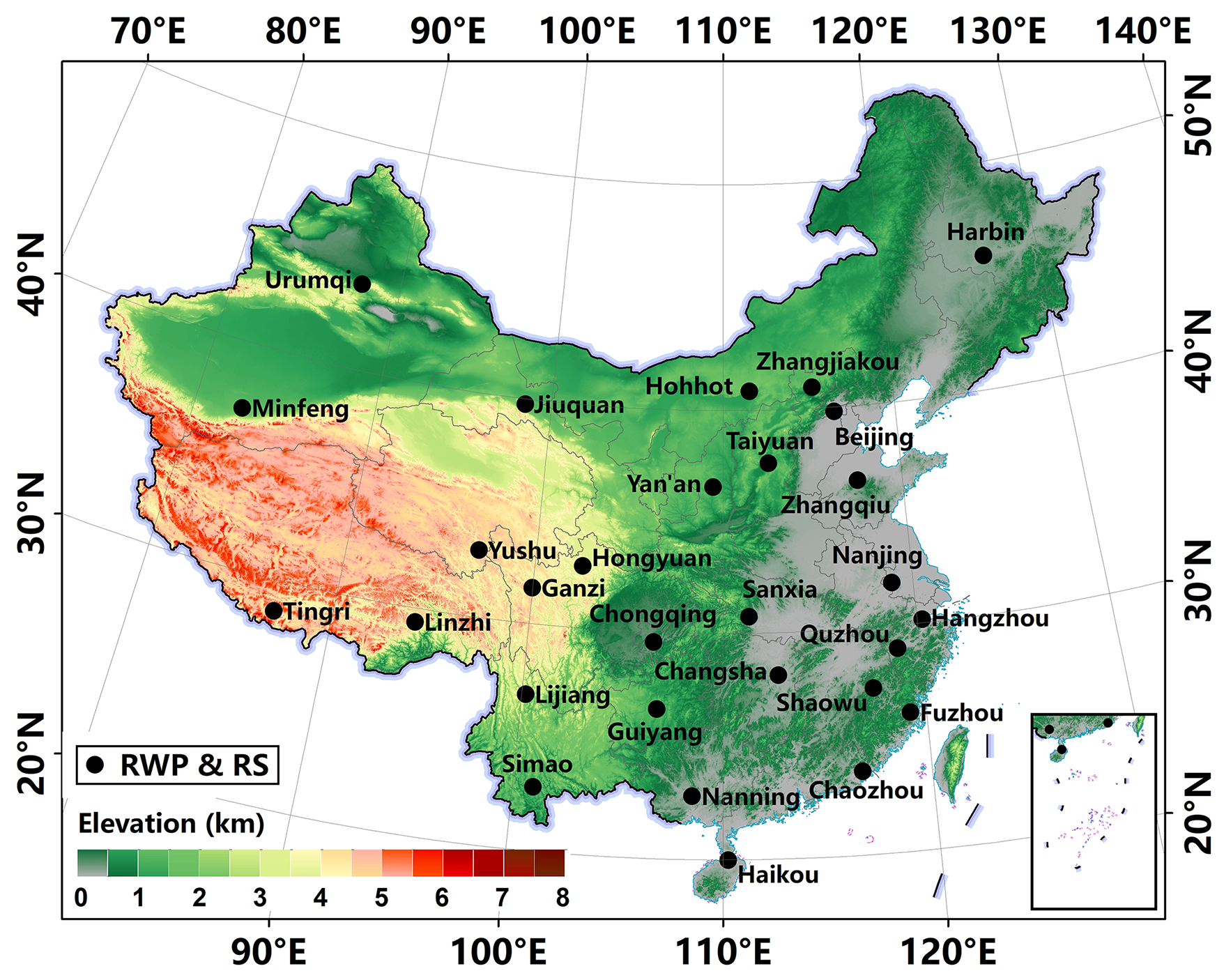
Figure 1 Spatial distribution of the collocated radar wind profiler (RWP) and radiosonde stations in China. Publisher's remark: please note that the above figure contains disputed territories.

Table 1 Summary of the radar wind profiler (RWP) stations used in the calculation of turbulence-related parameters.

The RWP system provides continuous wind profiling from 0.12 to 5.0 km a.g.l., with a temporal resolution of 6 min and a vertical resolution of 120 m within the low-level atmosphere. The system incorporates advanced signal processing techniques, including ground clutter suppression algorithms and adaptive spectral filtering, to mitigate ground clutter interference and enhance real-time data fidelity (Solanki et al., 2022; Guo et al., 2023).

The L-band radiosonde system delivers high vertical resolution profiles with a temporal resolution of 1 s and a vertical resolution of 5–8 m. Routine observations are conducted twice daily at 00:00 and 12:00 UTC. The radiosonde data undergo rigorous quality control and have been widely used in previous studies to examine spatiotemporal variations in turbulence and instability within the free atmosphere and PBL (Guo et al., 2016; Lv et al., 2021; Sun et al., 2025). Although horizontal displacement occurs between launch stations and balloon trajectories, the spatial exclusivity of these trajectories ensures non-overlapping sampling domains among stations. This spatial segregation, combined with high-density vertical profiling, enables statistically independent measurements of turbulence-related parameters at each station (Ko et al., 2024).

Prior to turbulence retrieval through RWP–radiosonde synergetic analysis, precipitation events were excluded using ground-based 1 min precipitation observations. Profiles from the RWP and radiosondes were synchronized to a 6 min time resolution, and data collected 30 min before and after precipitation events were excluded to minimize residual moisture effects on radar refractivity and balloon trajectory perturbations (Wu et al., 2024). This rigorous quality assurance process yielded 16 942 validated non-precipitation profiles, enabling statistically robust characterization of turbulence regimes across China.

2.2 Algorithms for the estimation of turbulence-related parameters

Figure 2 presents the flowchart illustrating the main steps involved in estimating the following turbulence-related parameters: N², ε, l₀, L_B, and K.

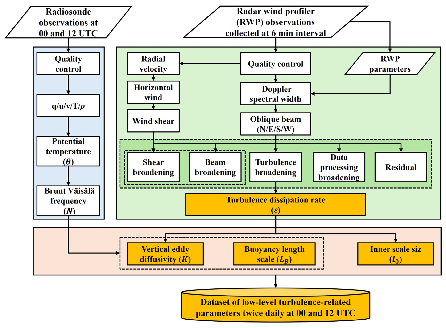
Figure 2 Flowchart used to generate the low-level atmospheric turbulence-related dataset at 00:00 and 12:00 UTC in China. Turbulence-related parameters include squared Brunt–Väisälä frequency (N²), turbulent dissipation rate (ε), inner scale (l₀), buoyancy length scale (L_B), and vertical eddy diffusivity (K).

N² is usually used as a parameter that indicates the stability of the stratification (s⁻²). It can be estimated based on the pressure and temperature profiles from radiosonde measurements (Lilly et al., 1974):

$$\begin{array}{}\text{(1)}& N^{\mathrm{2}}={\displaystyle \frac{g}{\mathit{\theta }}}{\displaystyle \frac{\partial \mathit{\theta }}{\partial z}},\end{array}$$

where g (units: m² s⁻¹) is the gravitational acceleration, z (units: m) is the altitude a.g.l., and θ (units: K) is the potential temperature, which is expressed as follows:

$$\begin{array}{}\text{(2)}& \mathit{\theta }=T{\left({\displaystyle \frac{\mathrm{1000}}{P}}\right)}^{\mathrm{0.286}},\end{array}$$

where T (units: K) denotes temperature and P denotes pressure (units: hPa).

ε represents the rate of energy cascading to smaller and smaller eddies until the energy is transformed into heat at the Kolmogorov scale (Fukao et al., 2014) and has units of m² s⁻³. ε can be estimated by the Doppler spectral width method (Nastrom, 1997). Turbulent spectral broadening (${\mathit{\sigma }}_{\mathrm{turb}}^{\mathrm{2}}$, units: m² s⁻²) is quantified by deducting non-turbulent broadening components (i.e., beam broadening, shear broadening, and transient effects) from the observed spectral width (σ_turb, units: m s⁻¹) (Dehghan and Hocking, 2011). The equation is as follows:

$$\begin{array}{}\text{(3)}& {\mathit{\sigma }}_{\mathrm{obs}}^{\mathrm{2}}\approx {\mathit{\sigma }}_{\mathrm{turb}}^{\mathrm{2}}+{\mathit{\sigma }}_{\mathrm{beam}+\mathrm{shear}}^{\mathrm{2}}.\end{array}$$

Beam and shear broadening (${\mathit{\sigma }}_{\mathrm{beam}+\mathrm{shear}}^{\mathrm{2}}$, units: m² s⁻²) is calculated using the following equations (Dehghan and Hocking, 2011):

$$\begin{array}{}\text{(4)}& \begin{array}{rl}{\mathit{\sigma }}_{\mathrm{beam}+\mathrm{shear}}^{\mathrm{2}}& ={\displaystyle \frac{{\mathit{\theta }}_{\mathrm{0.5}}^{\mathrm{2}}}{k}}{u}^{\mathrm{2}}\cos \mathit{\alpha }-a_{\mathrm{0}}{\displaystyle \frac{{\mathit{\theta }}_{\mathrm{0.5}}}{k}}\sin \mathit{\alpha }\left(u{\displaystyle \frac{\partial u}{\partial z}}\mathit{\zeta }\right)\\ & +b_{\mathrm{0}}{\displaystyle \frac{\mathrm{2}{\sin }^{\mathrm{2}}\mathit{\alpha }}{\mathrm{8}k}}{\left({\displaystyle \frac{\partial u}{\partial z}}\mathit{\zeta }\right)}^{\mathrm{2}}+c_{\mathrm{0}}{\sin }^{\mathrm{2}}\mathit{\alpha }{\cos }^{\mathrm{2}}\mathit{\alpha }\left|u\mathit{\xi }\right|\\ & +d_{\mathrm{0}}{\sin }^{\mathrm{2}}\mathit{\alpha }{\cos }^{\mathrm{2}}\mathit{\alpha }{\mathit{\xi }}^{\mathrm{2}},\end{array}\end{array}$$

where k=4ln 2, ζ=2Rθ_0.5sin α, $\mathit{\xi }=\frac{\partial u}{\partial z}\frac{\mathrm{\Delta }R}{\sqrt{\mathrm{12}}}$, a₀=0.945, b₀=1.500, c₀=0.030, and d₀=0.825 (Dehghan and Hocking, 2011). α is the beam zenith angle of the radar beam, θ_0.5 is the radar half-power beam width, R is the radar radial sampling distance (units: m), ΔR is the radial distance resolution, Δz is the vertical resolution, u (units: m s⁻¹) is the horizontal wind speed at R₀, and $\frac{\partial u}{\partial z}$ (units: s⁻¹) is the VWS at R₀.

ε can be expressed as a function of turbulence-induced spectral broadening through the following relationship:

$$\begin{array}{}\text{(5)}& \mathit{\epsilon }={\mathit{\sigma }}_{\mathrm{turb}}^{\mathrm{3}}{\left({\displaystyle \frac{\mathrm{4}\mathit{\pi }}{\mathrm{1.6}}}\right)}^{\mathrm{3}/\mathrm{2}}{J}^{-\mathrm{3}/\mathrm{2}}.\end{array}$$

The term J (m${}^{\mathrm{2}/\mathrm{3}}$) can be computed numerically with an estimate of the mean wind speed provided by RWP as follows:

$$\begin{array}{}\text{(6)}& \begin{array}{rl}& J=\mathrm{12}\mathrm{\Gamma }\left({\displaystyle \frac{\mathrm{2}}{\mathrm{3}}}\right){\int }_{\mathrm{0}}^{\frac{\mathit{\pi }}{\mathrm{2}}}d\mathit{\phi }{\int }_{\mathrm{0}}^{\frac{\mathit{\pi }}{\mathrm{2}}}{\sin }^{\mathrm{3}}\mathit{\psi }\left(b^{\mathrm{2}}{\cos }^{\mathrm{2}}\mathit{\psi }\right.\\ & {\left.+a^{\mathrm{2}}{\sin }^{\mathrm{2}}\mathit{\psi }+{\displaystyle \frac{L^{\mathrm{2}}}{\mathrm{12}}}{\sin }^{\mathrm{2}}\mathit{\psi }{\cos }^{\mathrm{2}}\mathit{\phi }\right)}^{\frac{\mathrm{1}}{\mathrm{3}}}d\mathit{\psi },\end{array}\end{array}$$

where Γ is the gamma function, $a=\frac{R{\mathit{\theta }}_{\mathrm{0.5}}}{\mathrm{4}\sqrt{\ln \mathrm{2}}}$ is the radius of the pulse volume, $b=\frac{\mathrm{\Delta }z}{\mathrm{8}\sqrt{\ln \mathrm{2}}}$ is the half-length of the pulse, L is the product of the mean wind speed and dwell time of the RWP during the sampling time, which can be expressed as u_tΔt, and a, b, and L have units of meters. The double integration is taken between 0 and $\mathit{\pi }/\mathrm{2}$ for both spherical coordinates ψ and φ (Solanki et al., 2022).

In the inertial subrange, l₀ (units: m) represents the scale for determining the transition region between the viscous and inertial subranges, and L_B (units: m) represents the scale for determining the transition region between the inertial and buoyancy subranges (Weinstock, 1978; Hocking, 1985; Fukao et al., 2014). L_B and l₀ can be computed as follows:

$$\begin{array}{}\text{(7)}& {\displaystyle }{L}_{\mathrm{B}}={\displaystyle \frac{\mathrm{2}\mathit{\pi }}{\mathrm{0.62}}}{\left({\displaystyle \frac{\mathit{\epsilon }}{N^{\mathrm{3}}}}\right)}^{\mathrm{1}/\mathrm{2}},\text{(8)}& {\displaystyle }{l}_{\mathrm{0}}=\mathrm{74}\cdot {\left(v^{\mathrm{3}}/\mathit{\epsilon }\right)}^{\mathrm{1}/\mathrm{4}},\end{array}$$

where v (units: m² s⁻¹) is the kinematic viscosity, $v=\mathrm{2}\times {\mathrm{10}}^{-\mathrm{5}}/\mathit{\rho }$, and ρ represents atmospheric density, which can be calculated based on the pressure and temperature profiles measured by radiosonde (Eaton and Nastrom, 1998; Solanki et al., 2022).

K is the ratio of kinematic heat flux to the mean potential temperature gradient (Weinstock, 1981b) and has units of m² s⁻¹. K can be calculated from the following equation:

$$\begin{array}{}\text{(9)}& K=\mathit{\gamma }\mathit{\epsilon }{N}^{-\mathrm{2}},\end{array}$$

where γ is the mixing efficiency, the value of which is empirically determined to vary between 0.2 and 1 (Fukao et al., 2014). $\mathit{\gamma }\approx R{i}_{\mathrm{f}}/(\mathrm{1}-R{i}_{\mathrm{f}}$), where Ri_f is the flux Richardson number, an important parameter in turbulence that is indicative of the ratio of buoyancy production to shear production (Fukao et al., 2014). A value of 0.25 corresponding to Ri_f=0.20 is used in this study (Clayson and Kantha, 2008).

3 Results and discussion

3.1 Horizontal distribution of turbulence-related parameters

The climatological analysis of the low-level turbulence regime below 3.0 km a.g.l. across China at 00:00 and 12:00 UTC in 2023 (Fig. 3) reveals distinct spatial patterns in turbulence-related parameters. Those turbulence-related parameters contain gradient Richardson number (Ri) (Guo et al., 2016), N², ε, K, L_B, and l₀. To examine the regional changes in the above-mentioned turbulence parameters, we divided China into four subregions: north China (NC), northwest China (NWC), south China (SC), and southwest China (SWC) (Fig. 3a).

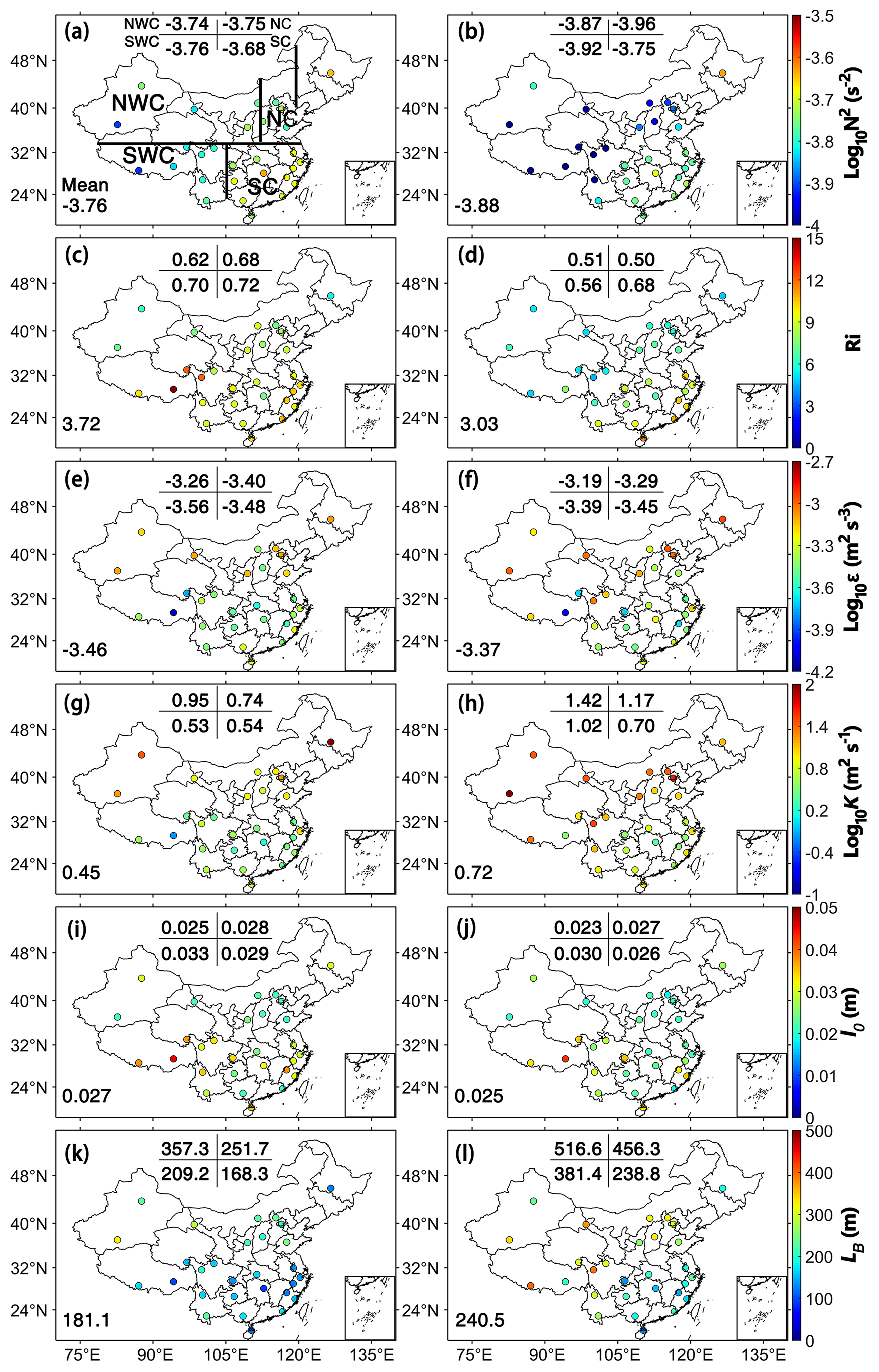
Figure 3 Spatial distribution and mean values of N² below 3.0 km a.g.l. in 2023 at (a) 00:00 UTC and (b) 12:00 UTC, (c, d) Ri, (e, f) ε, (g, h) K, (i, j) l₀, and (k, l) L_B. Here, China is divided into four subregions: north China (NC), northwest China (NWC), south China (SC), and southwest China (SWC). Publisher's remark: please note that the above figure contains disputed territories.

N² displays pronounced regional heterogeneity across China, characterized by enhanced static stability in SC and diminished stratification in NWC (Fig. 3a and b). This may be associated with the smaller Ri in NWC, indicating a more unstable atmospheric stratification (Fig. 3a–d). This instability may arise from intensified surface–atmosphere interactions driven by the unique environmental conditions over NWC, including elevated solar radiation flux due to reduced cloud cover, the predominance of bare soil and rock substrates with low albedo, and enhanced sensible heat flux from arid landscapes as compared to those in SC (Xu et al., 2021). As can be seen from Fig. 3e and f, turbulence is stronger in NC and NWC compared to SC by approximately 1 to 1.5 orders of magnitude, which may be related to stronger mechanically driven mixing from VWS and thermally driven convective mixing from surface heating (Chen et al., 2022b). The K shows a two-order amplification in NWC (Fig. 3g–h), governed by the synergistic enhancement of ε and N² through Eq. (9). This contrasts with SC's suppressed turbulence regime, where higher vegetation density and moisture increase atmospheric stability (Guo et al., 2016; Xu et al., 2021).

For the two turbulence scales, L_B demonstrates inverse spatial patterns compared to l₀ (Fig. 3i–l). L_B shows larger values across NC, NWC, and SWC, in contrast with smaller values in SC. Equation (8) indicates that L_B is proportional to ε and inversely proportional to N³, suggesting that smaller N², along with larger ε, contributes to a larger value of L_B. In contrast, l₀ demonstrates an opposite distribution compared to L_B (Fig. 3i and j). Since l₀ is proportional to ρ³ and inversely proportional to ε, lower ρ leads to larger l₀ values in SWC. As previously indicated, compared to SC, the strong sensible heat flux in NWC contributes to a more pronounced low-level turbulence characterized by larger L_B and smaller l₀ values.

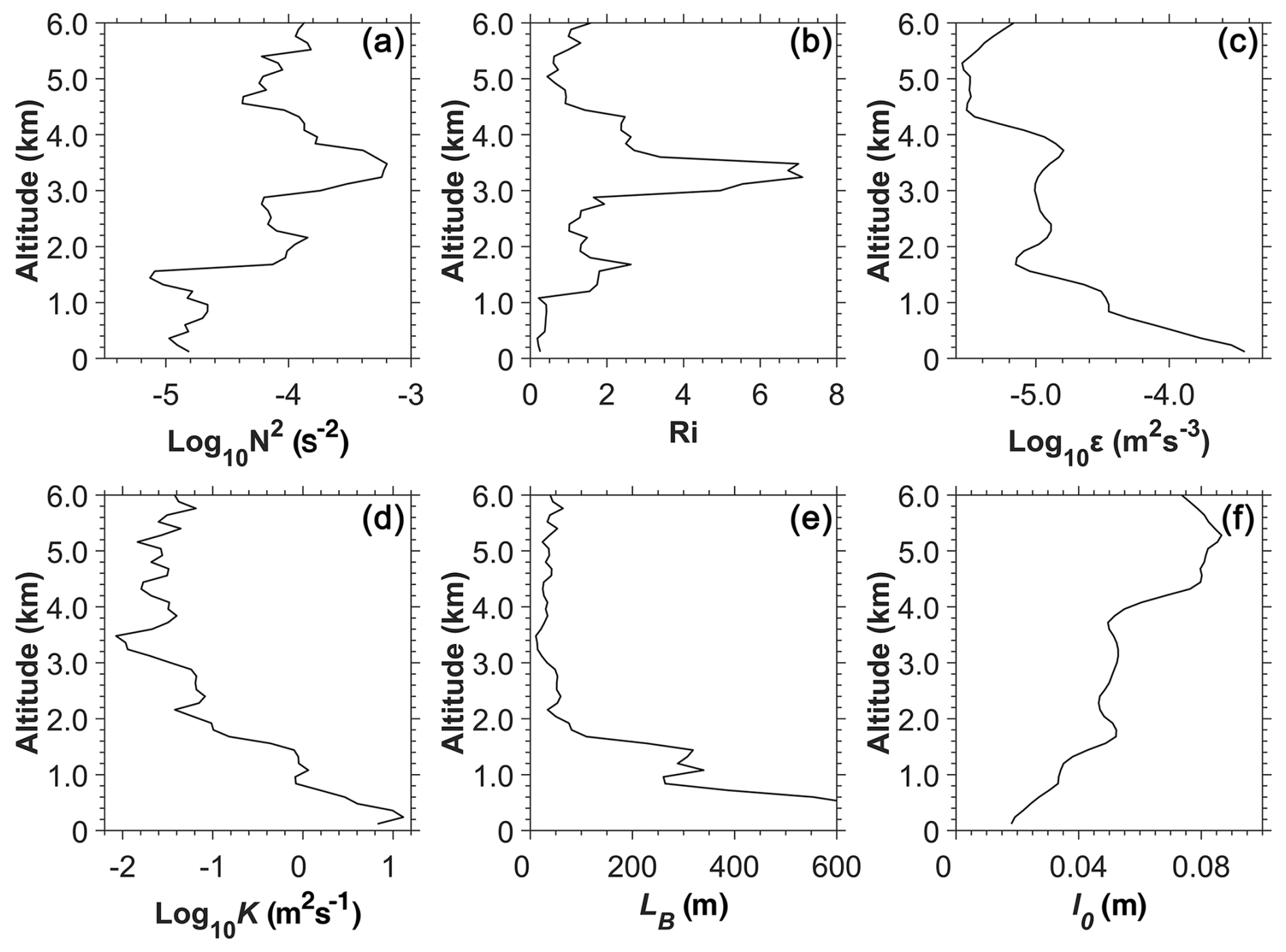
Figure 4 Vertical profiles of (a) N², (b) Ri, (c) ε, (d) K, (e) L_B, and (f) l₀ at 12:00 UTC for 16 July 2023 at Minfeng in northwest China. Note that N² is deduced from the sorted θ; it shows no regions of negative stability. However, Ri is inferred from the unsorted θ profile.

Further analysis reveals that the climatological mean values for N² are 10^−3.76 s⁻² at 00:00 UTC and 10^−3.88 s⁻² at 12:00 UTC, while the corresponding values for Ri are 3.72 and 3.03, indicating greater atmospheric instability at 12:00 UTC. Under a more unstable atmosphere, turbulence is stronger at 12:00 UTC, with climatological values of 10^−3.37, 10^0.72 m² s⁻¹, and 240.5 m for ε, K, and L_B, respectively. The enhancement in turbulence metrics at 12:00 UTC versus 00:00 UTC baseline originates from the delayed local solar noon in NWC (UTC + 6 zones) compared to SC (UTC + 8 zones). This leads to stronger turbulence (as shown in Fig. 3f, h) and larger maximum scale of eddy in the inertial subrange (Fig. 3l) in the NWC. Notably, low-level turbulence in SWC at 12:00 UTC exceeds those values in SC by ∼ 25 % (Fig. 3f, h, l), attributable to stronger surface heating over the Tibetan Plateau foothills and Taklamakan Desert.

3.2 Vertical structure and probability distribution function (PDF) characteristics of turbulence-related parameters

Figure 4a–f shows the profiles of N², Ri, ε, l₀, L_B, and K at 12:00 UTC on 16 July 2023 at Minfeng in NWC. It is evident that the vertical structure characteristics of N² and Ri are similar (Fig. 4a and b). Below 1.0 km a.g.l., N² is lower than 10^−4.60 s⁻² (Fig. 4a) and Ri is lower than 0.5 (Fig. 4b), which suggests static instability within the low-level atmosphere. In the altitude range from 1.5 to 3.0 km a.g.l., Ri exceeds 1, suggesting that an increase in static stability is a common feature. As shown in Fig. 4c–e, ε, K, and L_B display consistent vertical structure below 3.0 km a.g.l., characterized by a pronounced decreasing trend with altitude. ε varies from 10^−5.2 to 10^−4.0 m² s⁻³ (Fig. 4c), while K ranges from 10^−2.1 to 10^0.5 m² s⁻¹ (Fig. 4d) in the low-level atmosphere. L_B can reach up to 600 m at 0.5 km but decreases to around 50 m at 3.0 km a.g.l. (Fig. 4e). Conversely, l₀ increased with altitude, ranging from approximately 0.03 m at 0.5 km to about 0.06 m at 3.0 km a.g.l. (Fig. 4f). Reduced stratification N² and Ri synergistically intensify turbulent mixing within the low-level atmosphere and result in larger eddies in the inertial subrange. Furthermore, the intensity of turbulent motions and L_B diminishes with altitude, while l₀ increases (Ghosh, 2003).

Figure 5 demonstrates the vertical stratification through stability parameters (N², Ri), turbulence characteristics (ε, K), and turbulence scales (l₀, L_B) within the low-level atmosphere in 2023 across China. Below 1.5 km a.g.l., the values of N² and Ri at 12:00 UTC are markedly lower than those at 00:00 UTC (Fig. 5a and b), reflecting enhanced atmospheric instability. Log₁₀ε shows a nearly linear decrease with increasing altitude below 3.0 km (Fig. 5c), exhibiting gradients of −10^−3.70 m² s⁻³ km⁻¹ at 00:00 UTC and −10^−3.68 m² s⁻³ km⁻¹ at 12:00 UTC. This indicates stronger turbulence at lower altitudes with minimal differences in decay rates. Aligned with ε, K decreases with altitude at rates of −10^−0.14 m² s⁻¹ km⁻¹ (00:00 UTC) and −10^0.33 m² s⁻¹ km⁻¹ (12:00 UTC), further supporting reduced turbulent mixing at higher altitudes (Fig. 5d). Larger values of L_B are observed at lower altitudes, while the values of l₀ are larger at higher altitudes (Fig. 5e, f) (Ghosh, 2003; Rajput et al., 2022). L_B decreases sharply with altitude, showing steeper gradients at 12:00 UTC (−180.6 m km⁻¹) compared to 00:00 UTC (−69.6 m km⁻¹), consistent with stronger turbulence (Fig. 5f). This logarithmic decline suggests rapid attenuation of large turbulent eddies with altitude. In contrast, l₀ increases with altitude at rates of 0.0083 m km⁻¹ (00:00 UTC) and 0.0069 m km⁻¹ (12:00 UTC), reflecting a shift toward smaller-scale turbulence between the viscous and inertial subranges at higher altitudes (Fig. 5e). Marked vertical variability in L_B and l₀ dynamics reveals turbulence–stratification coupling mechanisms.

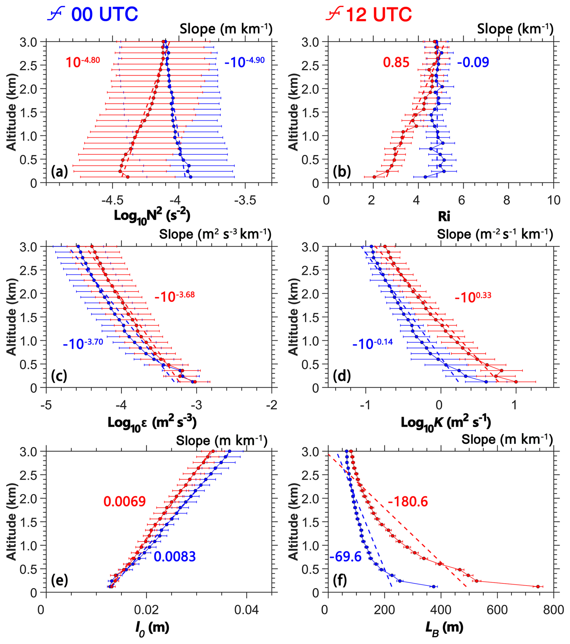
Figure 5 Vertical profiles of (a) N², (b) Ri, (c) ε, (d) K, (e) l₀, and (f) L_B in the 0.12 to 3.0 km altitude range a.g.l. at 00:00 UTC (blue) and 12:00 UTC (red) for 2023, and the slope values of turbulence-related parameters with altitude are also given in each panel where red and blue values represent 00:00 and 12:00 UTC, respectively.

Figure 6 presents the PDFs for low-level atmospheric stability parameters (N², Ri), turbulence metrics (ε, K), and turbulence scales (l₀, L_B). It can be observed that Log₁₀N² exhibits an approximately Beta-like distribution, with standard deviations of 10^−3.72 s⁻² at 00:00 UTC and 10^−3.78 s⁻² at 12:00 UTC (Fig. 6a). Ri displays characteristics of an approximate Gamma distribution (Fig. 6b), consistent with its sensitivity to shear-driven instabilities. Both ε and K show traits typical of log-normal distributions (Rajput et al., 2022), with standard deviations of 10^−3.11 m² s⁻³ (10^−3.07 m² s⁻³) for ε and 10^0.93 m² s⁻¹ (10^1.09 m² s⁻¹) for K at 00:00 UTC (12:00 UTC) (Fig. 6c–d). For the horizontal turbulence scale sizes, l₀ and L_B exhibit approximate Gamma distributions (Fig. 6e and f). l₀ exhibits standard deviations of 0.013 m and 0.012 m at 00:00 UTC and 12:00 UTC, respectively. L_B displays larger variability deviations of 219.8 m and 264.1 m at 00:00 UTC and 12:00 UTC, respectively. The distinct PDF shapes reflect fundamental differences in the statistical behavior of stability, turbulence, and mixing parameters. The near log-normal distributions of ε and K suggest Gaussian-like randomness in turbulent processes, while the Gamma and Beta-like distributions of Ri and Log₁₀N² align with their dependency on threshold-governed instabilities.

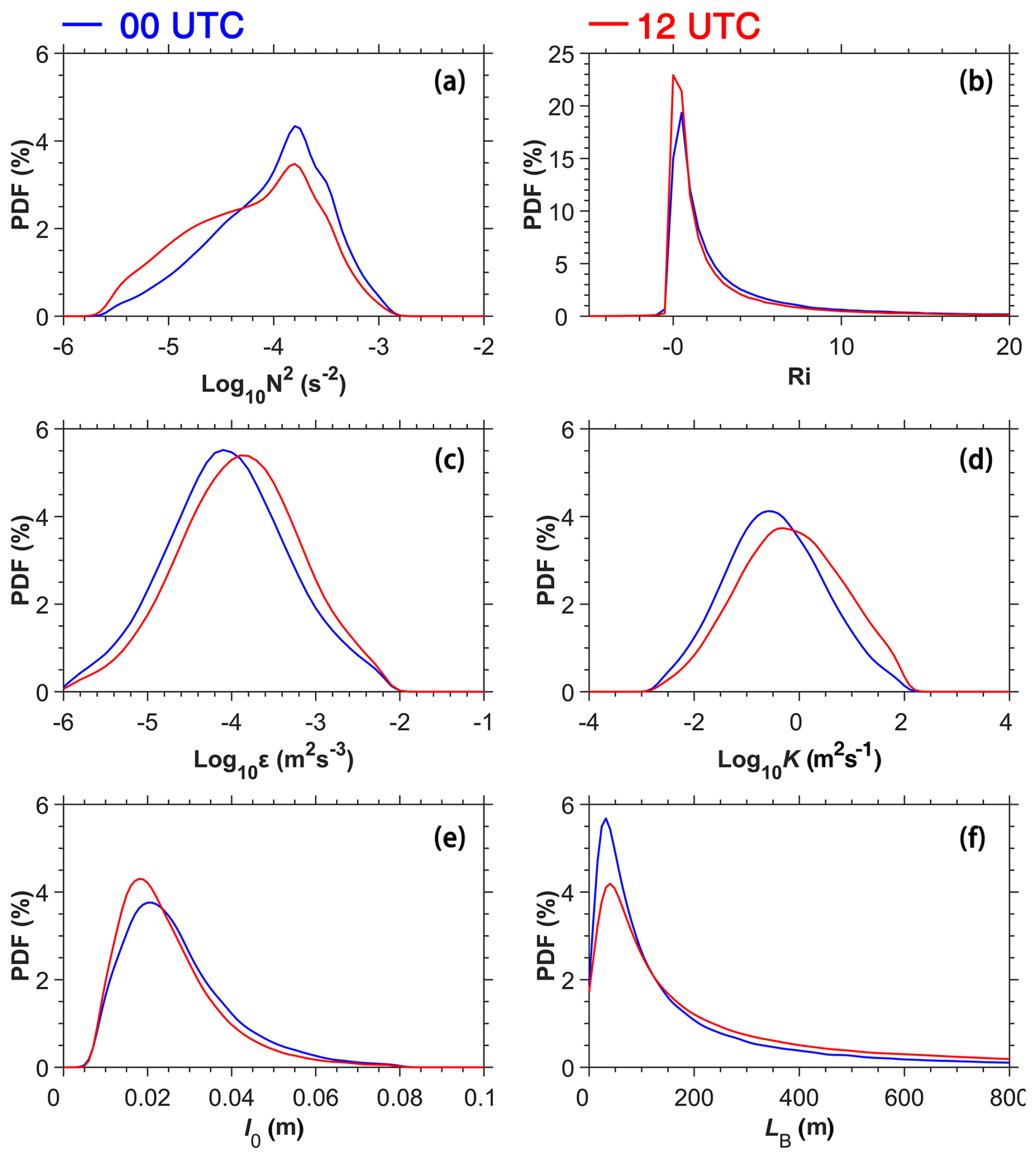
Figure 6 The probability density functions (PDFs) of (a) N², (b) Ri, (c) ε, (d) K, (e) l₀, and (f) L_B in the 0.12 to 3.0 km altitude range a.g.l. at 00:00 UTC (blue) and 12:00 UTC (red) for 2023.

Figure 7 demonstrates the relationships among turbulence-related parameters, with their quantitative correlation coefficients systematically presented at 00:00 and 12:00 UTC. Notably, Log₁₀N² and Ri exhibit strong covariation, reflecting progressive stratification breakdown during atmospheric destabilization. The correlation coefficients for Log₁₀ε with Log₁₀N² at 00:00 UTC (Fig. 7a) and 12:00 UTC (Fig. 7b) are −0.19 and −0.13, while the coefficients with Ri are −0.22 and −0.12, respectively. These values suggest that turbulence tends to be stronger in unstable atmospheric regimes. Log₁₀K demonstrates robust covariance with Log₁₀ε (R>0.80), whereas inverse mechanistic linkages emerge with stability indices (Log₁₀N² and Ri). L_B exhibits divergent relationships, showing positive correlations with turbulent metrics (R>0.65 with Log₁₀ε and Log₁₀K), while displaying inverse correlations with stability indices ($R<-\mathrm{0.45}$ with Log₁₀N² and Ri). The characteristic l₀ shows an inverse pattern to L_B with negative correlations to Log₁₀ε ($R<-\mathrm{0.80}$) and Log₁₀K ($R<-\mathrm{0.60}$) but positive correlations with Log₁₀N² and Ri. The interaction manifests as a marked negative correlation between L_B and l₀, with statistical confirmation of their anticorrelation pattern. These systematic correlations collectively suggest that atmospheric stability of stratification in the buoyancy subrange fundamentally modulates turbulent cascades and energy transfer processes through their coordinated effects on both buoyancy-dominated and shear-driven turbulent structures (Lotfy et al., 2019; Rajput et al., 2022).

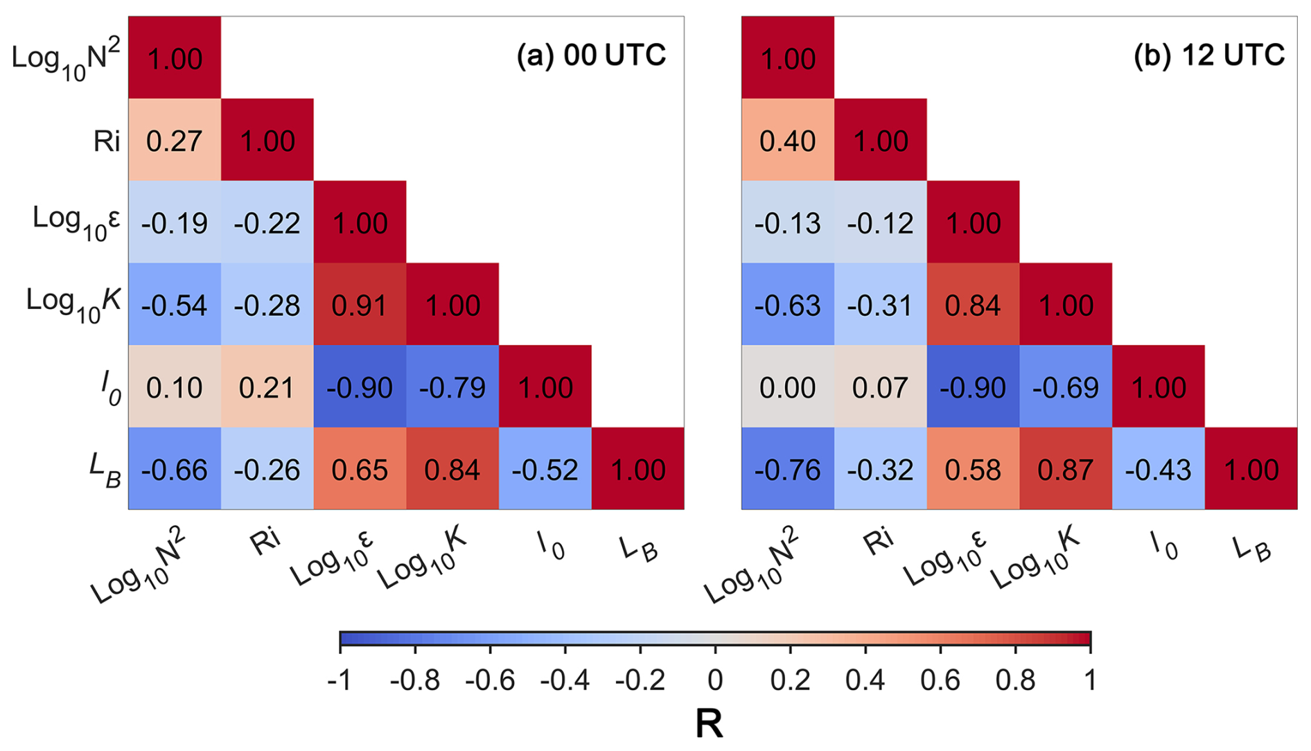
Figure 7 The correlation coefficients between turbulence-related parameters at (a) 00:00 UTC and (b) 12:00 UTC.

3.3 Seasonal variation of turbulence-related parameters with atmospheric stability

The previous subsection analyzed the spatial distribution and vertical structure of climatological turbulence-related parameters across China. This subsection focuses on the temporal turbulent variation in the low-level atmosphere.

Figures 8–9 systematically delineate interannual variability and seasonal cyclic patterns of N², Ri, ε, l₀, L_B, and K. N² is lower in spring and summer but higher in autumn and winter, indicating greater atmospheric instability during warmer months (Figs. 8a and b, 9a). In summer, N² reaches its minimum below 1.2 km a.g.l., indicating a more unstable stratification. Both ε and K exhibit higher values in spring and summer and lower values in autumn and winter, with an approximate increase of 1 order of magnitude during warmer seasons (Chen et al., 2022a) (Figs. 8c–f, 9c–d). L_B follows a similar seasonal pattern to ε and K (Figs. 8i–j, 9f), further supporting the link between turbulence intensity and turbulence scales in the buoyancy subrange. In contrast, the annual evolution of l₀ (Figs. 8g and h, 9e) is inversely related to ε and K, with smaller values in spring and summer and larger values in autumn and winter (Fig. 8g, h). The vertical profiles of ε, K, and L_B consistently decrease with altitude across all seasons, highlighting the altitude-dependent characteristics of turbulent processes.

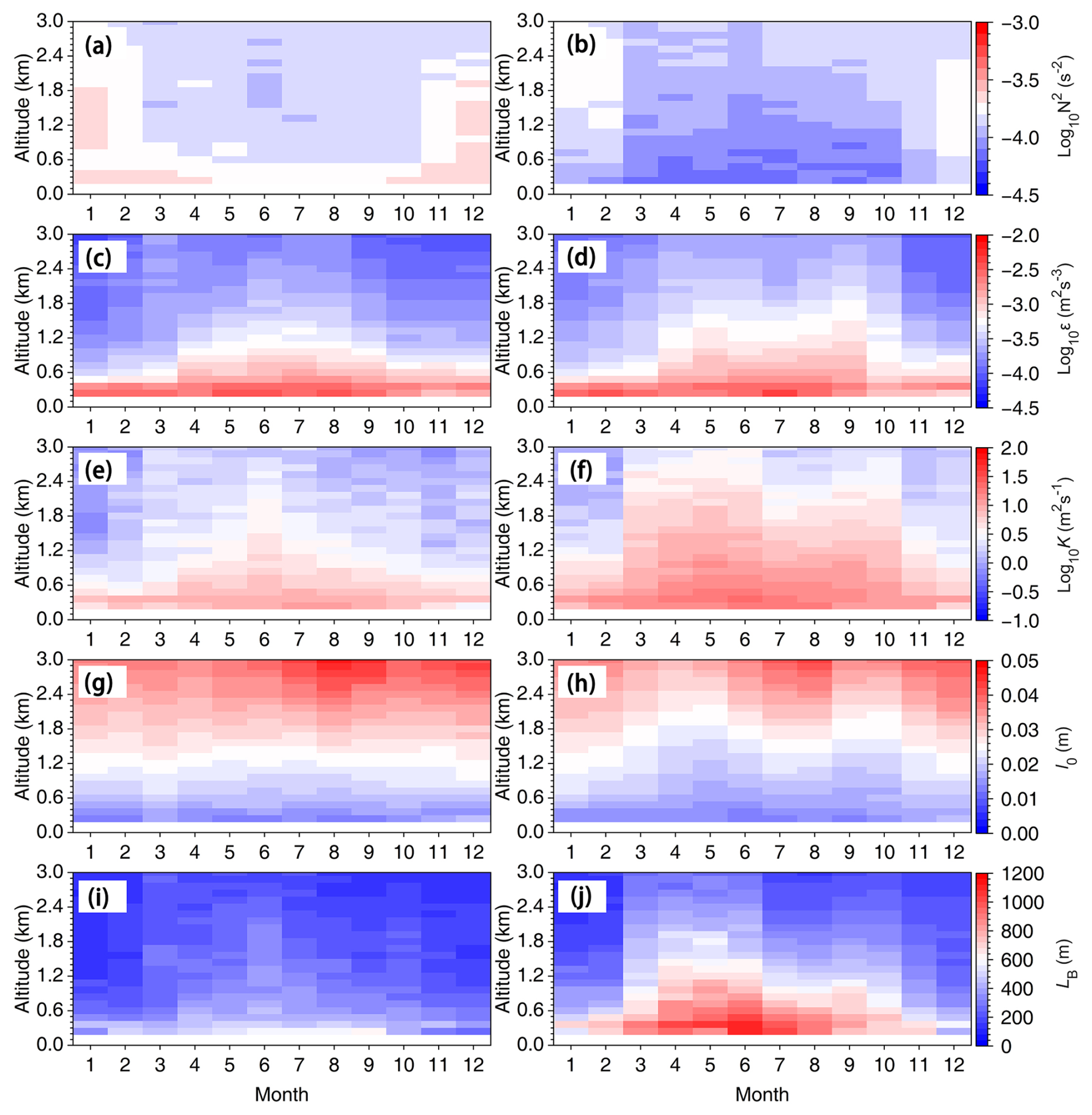
Figure 8 Monthly variation of (a) N², (b) Ri, (c) ε, (d) K, (e) l₀, and (f) L_B in the 0.12 to 3.0 km altitude range a.g.l. at 00:00 UTC (a, c, e, g, i) and 12:00 UTC (b, d, f, h, j) for 2023.

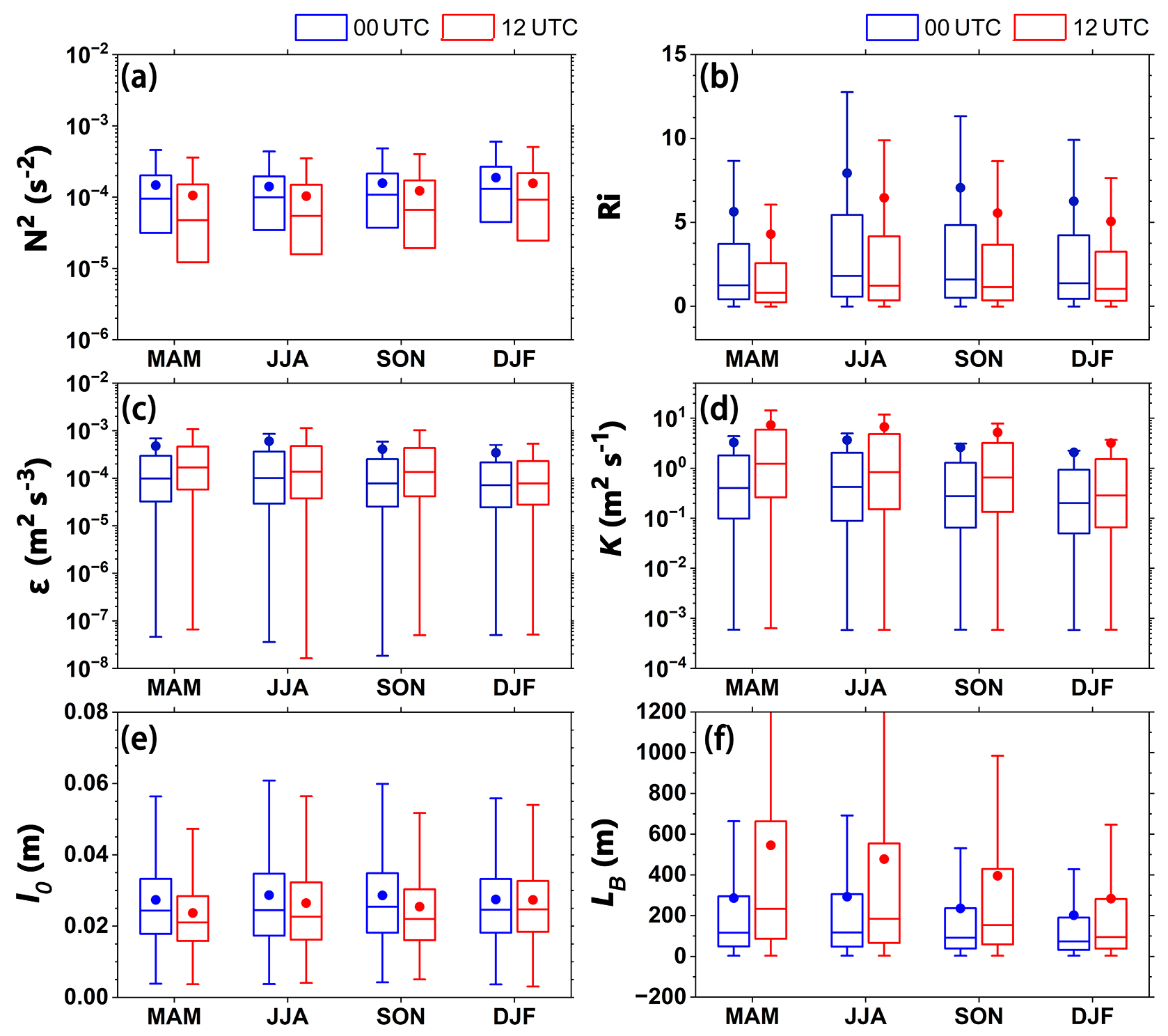
Figure 9 Box plot of seasonal (a) N², (b) Ri, (c) ε, (d) K, (e) l₀, and (f) L_B in the 0.12–3.0 km altitude range at 00:00 UTC (light blue) and 12:00 UTC (light red) for 2023. Note that the median is shown as a line, the mean value is displayed as a circle, while the outer boundaries of the boxes represent the 25th and 75th percentiles, and the lines represent the interquartile range (IQR). Seasonal divisions are MAM (March–May), JJA (June–August), SON (September–November), and DJF (December–February).

The seasonal evolutions of ε at 00:00 and 12:00 UTC are broadly similar, though ε is consistently stronger at 12:00 UTC, likely due to lower values of N² and Ri (Fig. 8a–b). In summer at 12:00 UTC, ε exceeds 10^−3.5 m² s⁻³ at an altitude of 1.8 km a.g.l., whereas in winter, this altitude is only reached at 0.6 km. This highlights the influence of seasonal turbulent dynamics on the development of the PBL. This suggests the existence of a maximum descent gradient region for ε and K at the PBL top (Meng et al., 2024). At 12:00 UTC, the l₀ values at 0.5 km are 0.012 m in summer and 0.013 m in winter, while at 1.2 km, those values are 0.021 m in summer and 0.024 m in winter (Fig. 8i). The values of L_B at 12:00 UTC are 910 m in summer and 550 m in winter at an altitude of 0.5 km (Fig. 8j). At 1.2 km, the values of L_B are 570 m in summer and 300 m in winter, which is approximately half of the values observed at 0.5 km. The seasonal variations in turbulence parameters underscore the critical role of atmospheric stability and PBL processes in modulating low-level turbulence intensity and mixing.

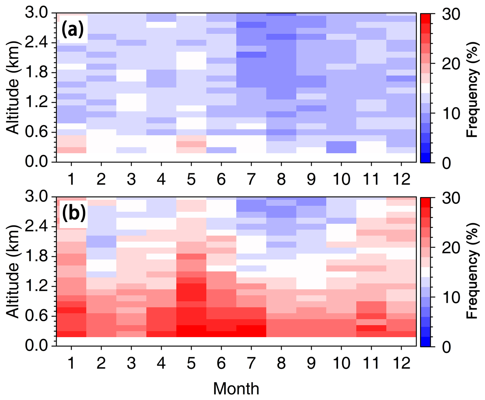
Figure 10 Monthly variation of the occurrence frequency of Ri<0.25 as a function of altitude, spanning from 0.12 to 3.0 km a.g.l. at 00:00 UTC (a) and 12:00 UTC (b) for the year 2023.

As previously discussed, the low-level atmosphere at 12:00 UTC exhibits greater instability compared to 00:00 UTC, resulting in stronger turbulence. However, it should be noted that 12:00 UTC corresponds to local standard time (LST) between 18 and 20, during which the PBL may exist in either a mixed or transitional state (Guo et al., 2016). To further investigate the relationship between turbulence structure and atmospheric stability at 12:00 UTC, this study adopted Ri<0.25 as an indicator of atmospheric instability (Chen et al., 2022a).

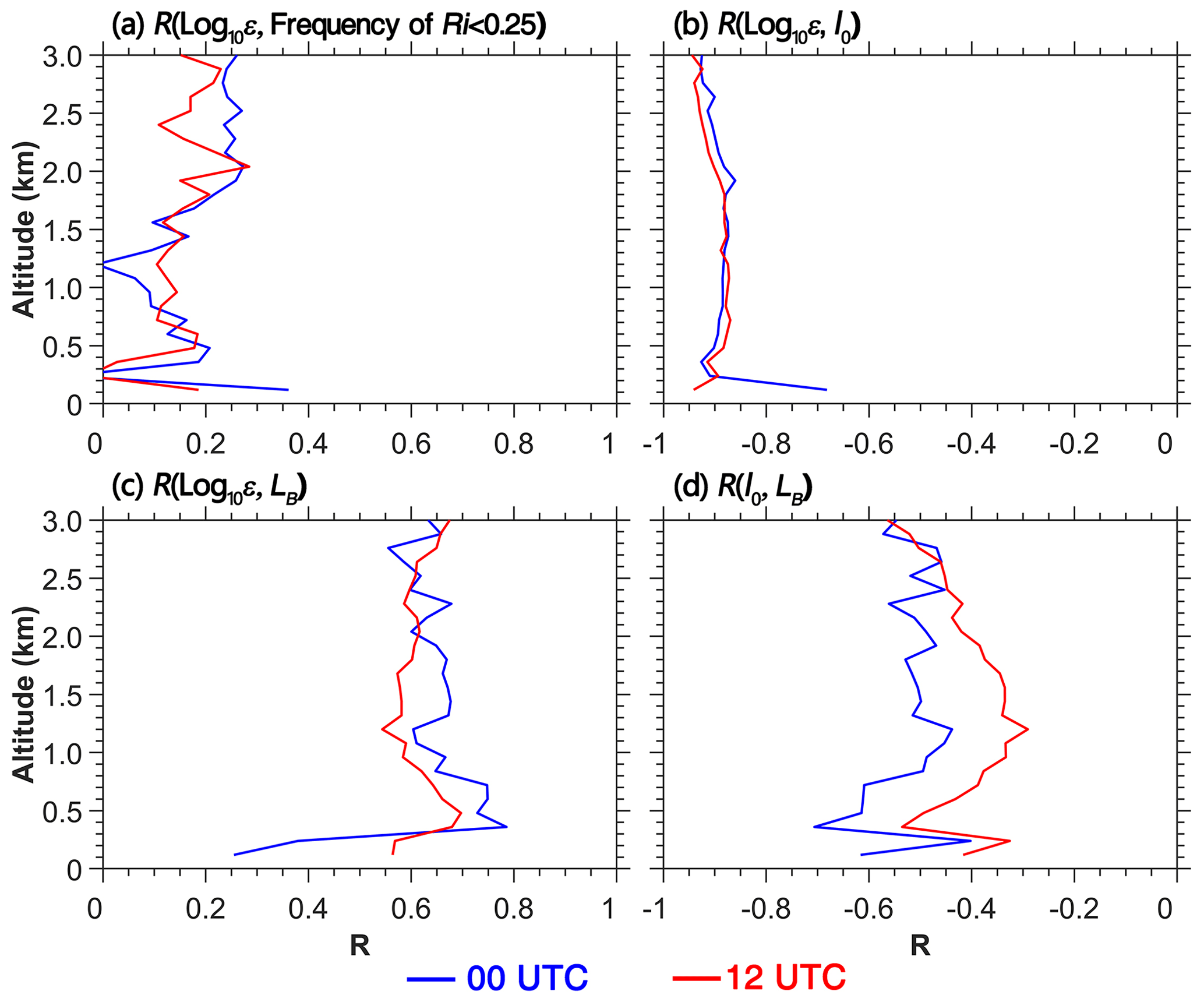
Figure 11 Profiles of correlation coefficient (R) between (a) Log₁₀ε and the frequency of Ri<0.25 at 00:00 UTC (blue) and 12:00 UTC (red). (b) Same as (a) but for the correlations of Log₁₀ε with l₀. (c) Same as (a) but for the correlations of Log₁₀ε with L_B. (d) Correlations between l₀ and L_B in the inertial subrange.

Figure 10 shows the vertical and seasonal distribution frequency of Ri<0.25 at 00:00 and 12:00 UTC. A distinct seasonal variation in the occurrence frequency is observed. Analysis of the occurrence frequency climatology reveals pronounced seasonality in low-level instability, with peak intensity and maximum eddies (L_B≈ 573.9 m) occurring at 12:00 UTC in May during the spring–summer transition period, dominated by enhanced thermal convection and synoptic-scale frontal activity (Chen et al., 2022a). This seasonal maximum coincides with weakened static stability and enhanced turbulence (Fig. 8), facilitating vigorous vertical mixing through buoyancy-driven plumes. Conversely, autumn–winter months exhibit suppressed turbulence and smaller L_B (minimum L_B≈ 272.6 m in January), corresponding to increased atmospheric stratification and reduced surface heat fluxes under frequent temperature inversion regimes (Xu et al., 2021).

Furthermore, a significant discrepancy exists between the occurrence frequency of Ri<0.25 at 00:00 and 12:00 UTC. For instance, in May, the vertical mean frequency of Ri<0.25 at 12:00 UTC is 23.6 %, whereas at 00:00 UTC it registers only 14.9 %. This disparity indicates a more unstable atmosphere and stronger turbulence at 12:00 UTC (Figs. 6d and 8c–f). Vertically, the frequency exhibits a decreasing trend with altitude, suggesting that the vertical structure of atmospheric instability contributes to the altitude-dependent attenuation of turbulence intensity (Figs. 5c–d and 8c–f).

Figure 11 presents the vertical structural distribution of correlations among turbulence-related parameters. Log₁₀ε shows positive correlations with the occurrence frequency of Ri<0.25 across altitudes (Fig. 11a), though Log₁₀K exhibits stronger correlations (not shown). This indicates that K responds more sensitively to atmospheric instability, particularly at 12:00 UTC, where the correlation coefficient exceeds 0.5 at 1.0–2.0 km a.g.l. As shown in Fig. 11b, l₀ demonstrates significant negative correlations ($R<-\mathrm{0.90}$) with Log₁₀ε vertically, suggesting that enhanced turbulence under lower atmospheric instability corresponds to smaller l₀ between the viscous and inertial subranges (Fig. 11b). Conversely, L_B shows significant positive correlations with Log₁₀ε, implying that stronger turbulence enlarges the maximum turbulent eddies between the inertial and buoyancy subranges (Fig. 11c). The correlation between l₀ and L_B is more pronounced at lower altitudes but remains relatively stable above 1.0 km. Hence, when the instability of the low-level atmosphere increases, the enhanced turbulence expands the range of the inertial subrange (Rajput et al., 2022).

4 Data availability

The low-level turbulence-related dataset in China can be accessed at https://doi.org/10.5281/zenodo.14959025 (Meng and Guo, 2025).

5 Summary and concluding remarks

The estimation of turbulence-related parameters can help improve the accuracy of short-term local weather forecasts. Despite its importance, detailed research on the structure of low-level atmospheric turbulence has been hindered by a lack of comprehensive observational data. This study aims to address this gap by investigating the temporal and spatial evolution patterns of low-level turbulence in China.

Using observational data from 29 collocated RWP and radiosonde stations across China, this research employs the Doppler spectrum width method to estimate critical parameters of lower-level atmospheric turbulence. These parameters include N², ε, l₀, L_B, and K. A comprehensive dataset of turbulence-related parameters was developed at the station scale for China in 2023, with a temporal resolution of 6 min and a vertical resolution of 120 m below 3.0 km a.g.l.

Spatially, low-level turbulence demonstrates significant geographical variability. Compared to SC, N² and l₀ are lower in NWC and NC, while ε, L_B, and K are higher. This indicates stronger turbulence in the NWC and NC. It can be concluded that the predominance of bare land with low soil moisture in NWC and NC results in higher sensible heat flux, promoting greater heat transfer to the PBL, more unstable atmospheric stratification, and stronger turbulence compared to the forested, high soil moisture regions of SC.

As altitude increases, ε, L_B, and K exhibit a decreasing trend, while N² and l₀ increase. The PDF of ε and K conforms to a log-normal distribution, whereas l₀ and L_B approximately follow a Gamma distribution. Temporally, turbulence-related parameters display pronounced seasonal variations, with stronger turbulence observed in spring and summer and weaker turbulence in autumn and winter. Additionally, turbulence intensity at 12:00 UTC is notably stronger than at 00:00 UTC, primarily due to the unstable atmospheric stratification with a larger occurrence frequency of Ri<0.25.

Although the dataset of low-level atmospheric turbulence-related parameters developed in this study encompasses typical regions across China, the limited station density and sparse radiosonde observations constrain the dataset's ability to provide high spatiotemporal resolution turbulence profiles for the entire country. In future work, additional data sources, such as coherent Doppler wind lidars and reanalysis datasets, will be integrated to construct a more refined, grid-scale turbulence dataset for China, enabling a more comprehensive understanding of atmospheric turbulence dynamics.