Statistical atlas of European agriculture: gridded data from the agricultural census 2020 and the spatial distribution of CAP contextual indicators

International organizations have voiced the need to integrate geographical information from agricultural holdings into official statistics to gain a better understanding of the spatial dynamics of the European agricultural sector. This paper presents a set of thematic maps based on the European 2020 agricultural census to explore the major structural differences between regions and countries. To comply with the confidentiality requirements associated with the census data, we applied a multi-resolution gridded approach by varying the resolution of the grid cells as a function of the density, dominance, and quality of individual observations. The datasets contain a mixture of grid resolutions ranging from 1 to 40 km, preserving a hierarchical structure where higher-resolution grid cells are aggregated into lower resolutions until the statistical disclosure requirements are met. The variables presented here correspond to the Contextual Indicators of the Performance Monitoring and Evaluation Framework of the Common Agricultural Policy and are divided into three broad categories: structural components (i.e., agricultural holdings, land use, livestock patterns, and labor input); the demographics of farmers (i.e., age, gender, and skills); and agricultural production methods (i.e., irrigation and organic farming). Our exploratory analysis indicates that high farm density occurs in plains, lowlands, and fertile soil in valleys; that high shares of organic farming tend to be concentrated in certain areas with high proportions of grassland; and that agricultural holdings managed by young farmers are located in a belt stretching from France through to Switzerland, Austria, Czechia, Slovakia, and Poland. These novel datasets are highly versatile, not only allowing policies to evaluate funding schemes at more local levels, but also offering researchers new opportunities to draw causal spatial inference from the multi-resolution gridded data. The dataset is the first attempt to create an unprecedented harmonized view of European agriculture with high spatial resolution and is available at https://doi.org/10.5281/zenodo.14852709 (Eurostat, 2025).

1 Introduction

The Common Agricultural Policy (CAP) is at the heart of European integration, reflecting the first attempt to create a single policy for an economic sector in the European Union (EU). While its objectives were enshrined in the Treaty of Rome in 1957, the cross-national harmonization of agricultural policy came into force in 1962 (Giuliani and Baron, 2023; European Commission, 2024c). The CAP was intended to mitigate against food shortages in Europe following the aftermath of World War II by implementing laws that would foster increases in agricultural productivity and self-sufficiency in food while stabilizing food markets and ensuring the availability of food at reasonable prices across Europe. Since then, the CAP has undergone several fundamental changes that have moved the CAP away from direct payments solely for agricultural production to a more diversified payment scheme that incentivizes sustainable management practices under the EU Green Deal (European Commission, 2019; Fettering, 2020).

The CAP has witnessed six major reforms in the last 30 years. The first reform under Ray MacSharry in 1992 aimed to reduce price support policies, causing trading conflicts with the main partners due to high production surpluses and the compensation payments introduced that were based on agricultural area or number of livestock (Beard and Swinbank, 2001; Sinabell and Schmid, 2017). A few years later, the European Commission presented the Agenda 2000 proposals for the CAP, in light of the preparation for the 2004 enlargement, continuing reductions in intervention prices for arable crops, beef, and dairy products with partial compensation in the form of direct payments. At the same time, Agenda 2000 was an initiative to open up the prospect of regionalization of rural policy, which was transformed into a second pillar of the CAP to reinforce the support for farm investments and agri-environmental and rural development measures (Papadopoulos, 2005). Important elements of the Luxembourg agreement in 2003 comprised the linking of direct payments to cross-compliance (i.e., rules on environmental protection, animal welfare, and plant health) and shifting funds from the market-oriented agricultural policy pillar to the second pillar by capping direct aid. In response to environmental concerns from nongovernmental organizations (NGOs) in 2013, the European Commission introduced greening payments, meaning that farmers only received direct payments if they complied with minimum standards on crop diversity, the preservation of permanent grasslands, and dedicated at least 5 % of their arable land to ecologically beneficial areas (e.g., hedges, nitrogen-fixing crops, fallow land) (Erjavec and Erjavec, 2015). In this current period of 2021-2027, about 30 % of the EU budget goes towards the CAP (European Parliament, 2023), with 6 out of 9 million farms receiving support (European Commission, 2024d). As part of recent CAP reforms, a more regional approach has been implemented in which EU Member States (MS) have produced national CAP strategic plans (European Commission, 2023a). Covering the period 2023–2027, MS have outlined how they plan to achieve the broader CAP objectives while taking into account the local context and conditions.

In parallel, a Performance Monitoring and Evaluation Framework (PMEF) has been developed for the CAP that uses a wide range of indicators to assess progress at the national level, as well as by administrative region using the nomenclature of territorial units for statistics, abbreviated as NUTS¹ (European Commission, 2023a).

A key input to the PMEF and previous CAP monitoring systems is data from the agricultural census and surveys, which involves the regular and systematic collection of data on the structure of a nation’s agricultural sector. Following the recommended methodology for agricultural censuses and surveys provided by the Food and Agriculture Organization of the United Nations (FAO) (FAO, 2017a, b), MS have conducted agricultural censuses every 10 years, as required by Regulation (EU) 2018/1091 of the European Parliament and of the Council of 18 July 2018 on Integrated Farm Statistics (IFS) (European Commission, 2018). Based on a common data collection methodology to ensure harmonization and comparability across MS, IFS is also used to monitor the state of agriculture more generally, with a myriad of applications that have been performed, such as a review of the environmental risks of agriculture (Delbaere and Nieto Serradilla, 2004), the investigation of labor productivity in different agricultural systems in Europe (Giannakis and Bruggeman, 2018), and the development of a crop-specific European irrigation map (Wriedt et al., 2009; Zajac et al., 2022).

The last agricultural census took place in 2020, collecting more than 300 variables on agriculture and farm structure from 9 million farmers in the EU (and EFTA countries Iceland, Switzerland, and Norway). Data from the IFS are aggregated to NUTS 2, NUTS 1 or national levels before they are publicly released on the Eurostat website due to confidentiality regulations that do not allow individual data to be disclosed (European Commission, 2018). During the previous CAP period (2014–2022), the Common Monitoring and Evaluation Framework (CMEF) developed a set of context indicators which take the form of quantifiable variables used to assess overall policy performance and provide information on structural, economic, and environmental trends. Most indicators have used IFS data (European Commission, 2023c) and can be viewed on the EU Agridata Portal² (see, for example, context Indicator C17 on Agricultural Holdings) (European Commission, 2023b). Most of the information related to context indicators is presented at the national level, although some of the maps display information in NUTS 2 administrative zones. However, NUTS 2 regions are too coarse and mask the large structural disparities within NUTS 2 regions that are not identifiable using such data. To more effectively monitor and evaluate the implementation of the CAP, and to guide the design of future funding schemes, more highly resolved spatial information from agricultural censuses and surveys is needed. This would also benefit many other applications and models that need high-resolution input related to the agricultural sector.

Few attempts have been made to create interactive cartography in the form of an agricultural atlas with information and data showing single agricultural indicators at a finer level of resolution. A notable example is the Agrarian Atlas (see https://agraratlas.statistikportal.de/, last access: 30 May 2025) disseminated by the German statistical office, which provides a range of agricultural variables on a 5 km grid. The layers are accessible through a web coverage service (WCS) but only by the aggregated classes as they appear in the atlas and not by the raw data. Gridded agricultural data are also available for the UK at resolutions of 2, 5 and 10 km hosted by the University of Edinburgh (see https://agcensus.edina.ac.uk/, last access: 15 May 2025) (EDINA), but free access is only available for academic institutions; otherwise, the data must be purchased.

Other examples of gridded agricultural data are those that are down-scaled to a resolution of around 10 km based on data originally disseminated at the level of administrative zone. This includes FAO's Gridded Livestock of the World, which provides gridded livestock numbers for 2010 and 2015 (Gilbert et al., 2018, 2022) and crop types from the Spatial Production Allocation Model (SPAM) dataset for 2010 (Yu et al., 2020). Gridded data on crop types are also available from EarthStat, a collaboration between two universities from the United States, for the year 2000 (Ramankutty et al., 2008), which has been updated for the year 2020, named as the CROPGRIDS product (Tang et al., 2024), and includes other gridded layers, such as the application of nutrients for major crops. In addition, the World Bank provides a catalog of gridded datasets, including global gridded agricultural gross domestic product (World Bank, 2023). The disadvantage of these down-scaled datasets is the uncertainty related to estimated values from models instead of employing aggregations from actual census data.

To fill these gaps, we developed a method for gridding agricultural census data that employs a flexible, multi-resolution grid cell approach. This procedure can present the data at a much higher resolution than NUTS 2 while respecting the statistical disclosure requirements for confidentiality that protect the identities of individual farms (Skøien et al., 2025). The resolution of the grid varies from a minimum of 1 km (based on the Infrastructure for Spatial Information in Europe (INSPIRE) Statistical Units Grid for pan-European data) to 40 km, which is the maximum size that nullifies the disclosure risk while maximizing the utility of the information content presented.

By applying this new approach to the variables in the 2020 IFS, we now have an unprecedented and harmonized view of European agriculture compared to previous analyses carried out at the coarser NUTS 2 level. To illustrate this innovation, we have selected key variables from the 2020 IFS that are relevant to the CAP containing information on structural components (i.e., agricultural holdings, land use, livestock pattern and labor input), the demographics of farmers (i.e., age, gender, and skills), and agricultural production methods (i.e., irrigation and organic farming). These datasets are publicly accessible through an interactive map viewer called Gridviz³, which is publicly accessible from the Eurostat Experimental Statistics web page (https://ec.europa.eu/assets/estat/E/E4/gisco/farmstatistics/index.html, last access: 2 June 2025). The gridded data from the different layers are available at https://doi.org/10.5281/zenodo.14852709 (Eurostat, 2025).

Eurostat and MS coordinate the organization of agricultural surveys and censuses in the IFS Working Group. The release of geospatial data was approved in November 2024 by all countries except Germany. For this reason, we had to exclude the data from Germany in this paper. Eurostat and Germany are working together to overcome secondary confidentiality concerns and hope to release German IFS data within these EU spatial data layers as soon as possible. Overall, it is clear that such a statistical atlas of European agriculture provides new opportunities for policy evaluation, assessment, analysis, and the creation of land use related maps at high spatial resolution.

2 Methods

This section provides further information about the data collected at EU level and the context indicators that have been selected to produce the statistical atlas of gridded layers using the multi-resolution approach.

2.1 Agricultural census data and CAP context indicators

While the decennial census of agriculture forms the backbone of agricultural statistics, in addition it also constitutes a unique statistical source that covers the broadest spectrum of agricultural holdings⁴ in the EU to aid the development of the CAP. Data collection aims to produce harmonized, coherent and comparable statistics to meet current policy and emerging user needs (Lampach and Maríınez-Solano, 2023; Selenius et al., 2021). These statistical requirements are laid down in the Regulation (EU) 2018/1091 on IFS by establishing a coverage of 98 % of the utilized agricultural area (UAA) and 98 % of the livestock units (LSU) for the main structural agricultural variables, named core,⁵ such as land use, livestock patterns, economic size, farmer characteristics, or production methods (European Commission, 2018). Where the frame does not meet these requirements, the MS should extend the frame by establishing lower physical thresholds than those specified in Annex II of the legal basis. While countries have the obligation to fulfill this condition with respect to the coverage of the core variables, it is not mandatory to collect data on specific topics, called modules, or for the composition of the agricultural labor force of agricultural holdings or information related to soil management practices, manure management, or animal housing. To reduce the burden on countries, samples can be carried out to gather relevant data on specific topics according to the precision requirements of Annex V of the legislation.

Table 1 summarizes the number of holdings and the coverage of the agricultural holdings for each country in the 2020 agricultural census. It should be noted that the share of coverage can exceed 100 % as the total UAA and the total LSU are subject to variations, as these values are determined prior to data collection in the period t−1. Particularly interesting is that a number of countries (e.g., CY, ES, IT, MT, RO, SI, NO) cover their entire agricultural area and animal stock with the IFS survey. On the other hand, we observe that most countries satisfy the main coverage conditions (98 % UAA and 98 % LSU) when referring to samples that meet at least one of the physical thresholds (e.g., UAA is greater than 5 ha, number of bovine animals is greater than 10 head).

National data providers (i.e., national statistical offices, agricultural ministries, or other governmental bodies) prepare the questionnaire, conduct interviews, and complete the survey with additional information from administrative registers (e.g., wine, bovine herd, integrated information, and the control system). Individual records at the farm level are encrypted and transmitted to Eurostat through a secure system that implements an automated procedure to validate the content and structure of the microdata.

Table 1 Coverage of the 2020 agricultural census in terms of utilized agricultural area (UAA), excluding kitchen gardens, and livestock units (LSU) for each country. Country abbreviations are given in Table A2.

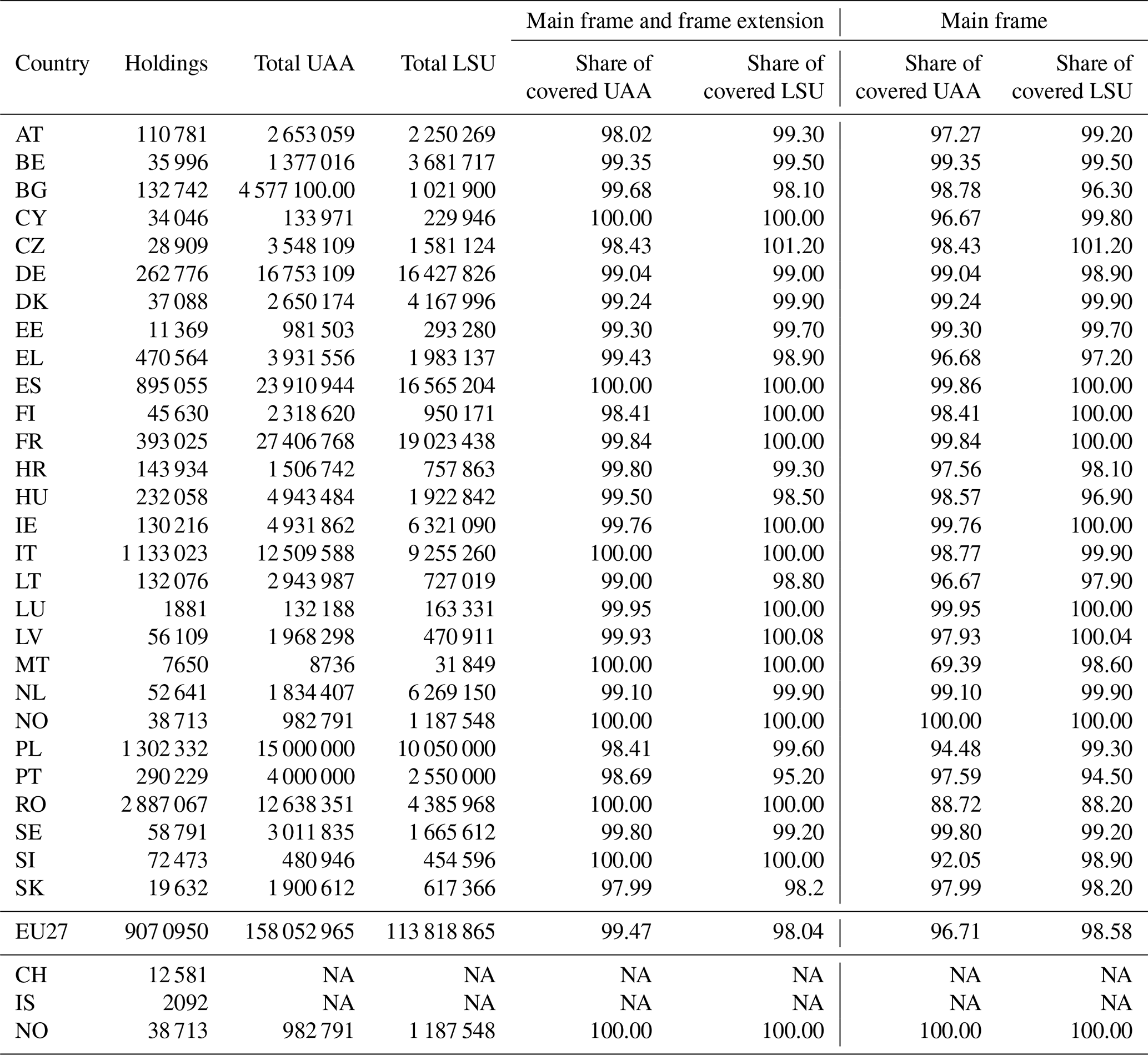
Note: incomplete quality reports from CH and IS cause missing information on total area and LSU. Source: European Commission (2024e). NA – not available.

The 2020 agricultural census was carried out during the COVID-19 pandemic, posing significant challenges for countries to meet the official deadline of the data collection period. Although some countries did not experience an impact from the pandemic due to the early adoption of information and communication technologies (e.g., computer-assisted data collection mode, administrative registers), other countries were negatively affected, particularly those that could not conduct face-to-face interviews due to social distancing restrictions.

However, these exceptional circumstances also motivated around a third of these countries to adopt remote data collection methods (e.g., computer-assisted telephone/web interviewing, data collection by post).

Table 2 Overview of contextual indicators in the framework of monitoring the Common Agricultural Policy (CAP).

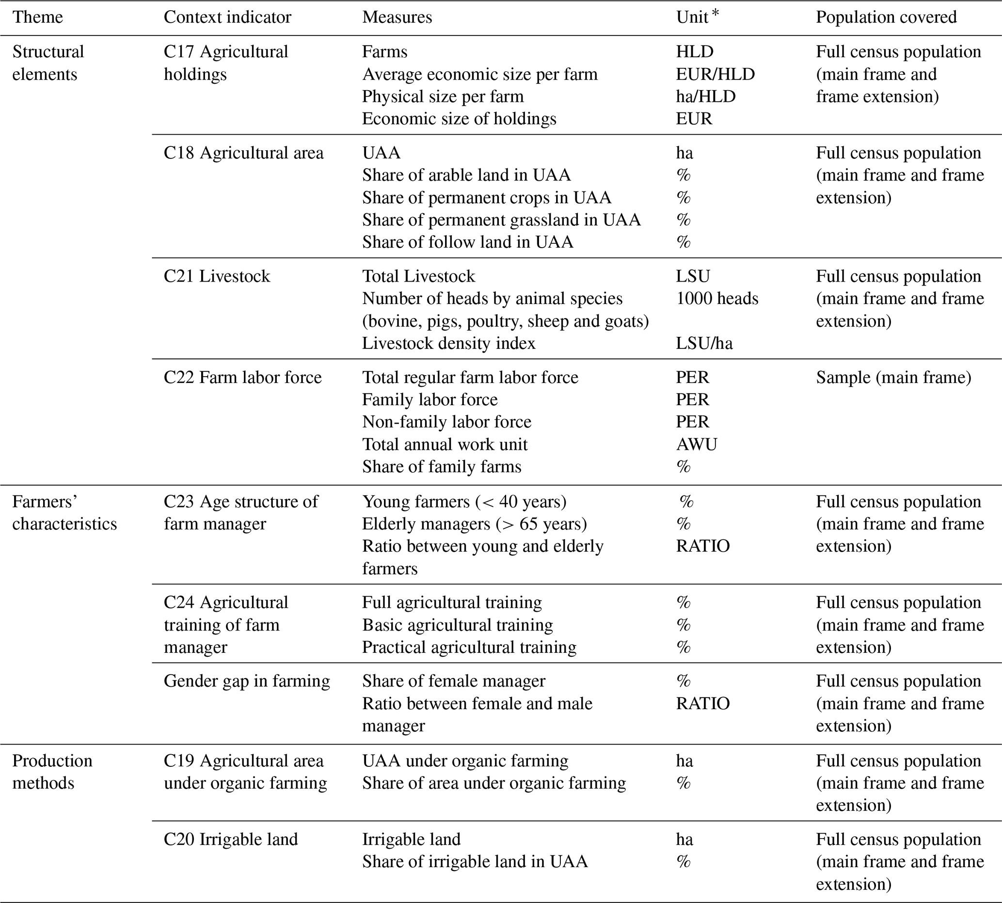
^* Abbreviations in the “Unit” column are as follows: ha – hectares; HLD – holding; EUR/HLD – euros per holding; EUR – euros; LSU – livestock unit; LSU/ha – livestock units per hectare; PER – people; AWU – annual work unit; RATIO – ratio.

As outlined in the introduction, the CAP is evaluated using a set of indicators, some of which are derived from the IFS. In addition to the indicators in the CMEF for the period 2014 to 2022 and the new framework of indicators that is used for the current CAP period (PMEF), there are also context indicators. These are used to provide a more general picture of the agricultural sector and rural areas, as well as trends in the economy and environment (European Commission, 2025). In the past, these context indicators have only been provided at the aggregated level of NUTS 2 or NUTS 3.

In this paper, we have selected the context indicators that are relevant to the agricultural sector and present them for the first time as high-resolution gridded layers based on the 2020 IFS. The indicators have been organized into three main categories: structural components, farmer demographics, and agricultural production methods. The specific indicators within each component are described in Table 2.

2.2 A multi-resolution gridded approach for statistical disclosure control and quality rating

There are different approaches available that can be used to grid census data while ensuring that confidential information from individual units is sufficiently masked. According to Implementing Regulation (EU) 2018/1874 on IFS and a series of recommendations from Eurostat (2020) on confidentiality rules, values cannot be disseminated on a 1 km grid when the cell includes fewer than 10 agricultural holdings (i.e., the threshold rule), the two largest values in the grid cell contribute more than 85 % of the total value of the grid cell (i.e., the dominance rule), or the value does not satisfy certain quality criteria (i.e., data accuracy is evaluated based on sampling errors that can be estimated from the sample itself using the standard errors of the estimated values. If the coefficient of variation of the estimated values is greater than 35 %, the cell is usually suppressed). Alternatively, aggregating to a nested 5 km or larger grid size is required to meet these rules.

The most common approach is a regular grid with a single resolution. However, to comply with the confidentiality rules in every grid cell, a coarser resolution grid would be required, even in locations where a higher resolution could be used. This comes from the fact that the confidentiality rules must be satisfied in all locations. Instead, a higher-resolution grid size could be chosen, but it will result in little avail due to the suppression of many small grid cells causing information loss. For example, EDINA releases three versions of its agricultural census data from the highest resolution at 2 km to the coarsest at 10 km (Macdonald, 2004). Since these data are released at a single grid size, the data are suppressed in many areas where the disclosure requirements are not met or are less reliable (Khan et al., 2013). Hence, in these gridded approaches, there is a trade-off between the choice of resolution and data utility.

Instead, it is preferable to produce a gridded dataset with a variable grid size that is organized in a hierarchical structure, i.e., grid sizes that are multiples of the smallest grid size. This approach is referred to as a multi-resolution grid or a quadtree (Samet, 1984; Skøien et al., 2025), which is a data structure used for the efficient storage of spatial data and images. The resolution of the grid will vary on the basis of the underlying density of the observed values in such a way that the confidentiality rules and the quality criteria of the estimated values are respected for all grid cells.

Figure 1 gives a broad overview of the methodology developed by Skøien et al. (2025) and implemented in the open source R package MRG that is applied to produce the gridded dataset (IFSGRID) and the maps in Sect. 3.1.

The values in Fig. 1 refer to the number of farms per grid cell; we only consider the threshold rule (i.e., at least 10 farms need to be in a grid cell) in this example for the sake of brevity (see Fig. A2 in Appendix A explaining more in detail the iterative process of producing a nested structure of multiple grids satisfying a set of confidentiality rules and quality requirements). The procedure for the compilation of multi-resolution grids in compliance with the confidentiality rules can be summarized as follows:

1. All records are aggregated to the highest grid resolution (1 km in the case of IFS data), as shown in the left panel.

2. Grid cells that do not respect the confidentiality rules will be aggregated with their neighbors to larger grid cells (5 km for IFS, but only double for this simplified example) (central panel).

3. Grid cells that still do not respect the confidentiality rules will be aggregated with their neighbors to larger grid cells (right panel). This step is repeated until there are no more confidential grid cells or until a maximum grid cell size has been reached. Grid cells that are still confidential need to be suppressed.

4. As an alternative, the method allows for a contextual suppression of grid cells. This means that grid cells that have a small value compared to the new and aggregated grid cells will be suppressed instead of aggregated to a lower level of resolution. This would be the case for the lower left corner in the lower right panel, where it might be better to keep the intermediate resolution with data for one grid cell, rather than creating a larger cell that only has one more farm. Typical suppression limits would be 0.02 or 0.05, whereas the grid cell in the lower right panel would be suppressed if the limit is more than $\mathrm{1}/\mathrm{12}$ (where 1 is the value to be suppressed and 12 the total value of a potentially merged grid cell.

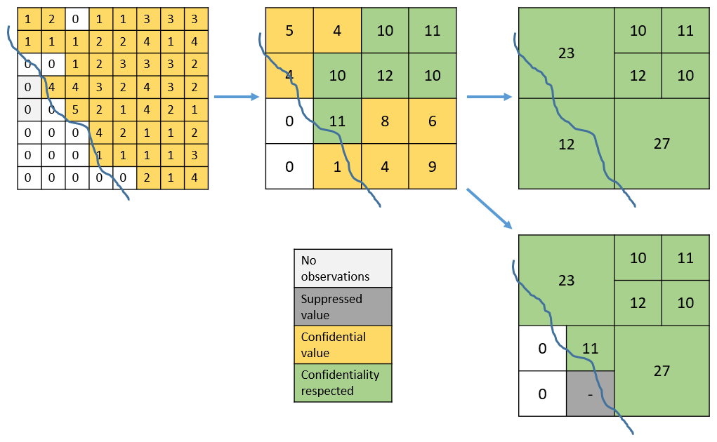
Figure 1 Illustration of the creation of multi-resolution grids in compliance with the confidentiality rules.

Several parameters related to the confidentiality rules, the quality rating, the suppression limit, the set of resolutions, and the rounding method can be defined by users. The default parameters follow the recommendations of Eurostat (2020) and the Implementing Regulation (EC) 2018/1874 as mentioned above. The suppression limitation parameter was set to 0.05, which means that if a grid cell contributes less than 5 % of the total aggregated new grid cell at a lower-resolution level, it will be suppressed to maximize the utility of the data. In addition, it is also possible to add customized user-defined functions for other possible restrictions, such as a confidentiality rule depending on another or multiple variables.

In Sect. 3.2 we demonstrate the added value of higher-resolution maps by comparing gridded data with tabular data for specific NUTS 2 regions. We carried out a statistical analysis that demonstrates the divergences between the value of the average aggregated value and the individual grid cell within a specific NUTS 2 region in Europe.

Figure 2 Example of consolidating two gridded datasets to a common multi-resolution grid.

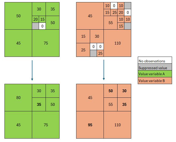
Although the creation of multi-resolution grids of standalone maps can be informative to identify common patterns, it is widely recognized that the temporal and spatial comparison of distinct maps is impeded due to heterogeneous grid sizes. To analyze the relationships between two spatially gridded variables, we have developed a procedure to consolidate grids from different datasets with different resolution grid sizes in a given location (see Skøien et al., 2025 for more details on the methodology and see https://github.com/jskoien/mrg, last access: 2 June 2025, for the implementation in the open source software R). The final grid cell sizes in the common resolution is the lowest available resolution from the selected maps and smaller grid cells from one map will be aggregated to the required resolution level. Figure 2 presents an example showing the consolidation of two indicators. For example, the upper left part in the upper left panel (i.e., the small grid cells) of the multi-resolution grid data for indicator A is aggregated to a lower-resolution level. In the end, both datasets contain the same common multi-resolution grids, allowing for statistical correlation and spatio-temporal analysis.

This conservative approach nullifies the risk of disclosing confidential information when consolidating different multi-resolution grids datasets. The outcome of the merger depends on whether the data are post-processed (i.e., rounding is applied or cells are suppressed due to noncompliance with the confidentiality rules). To present the potential of this approach, we examine the relationship between two indicators in Sect. 3.3.

3 Results and discussion

The results are divided into three main sections. In Sect. 3.1, we provide examples of a range of indicators from Table 2, showing the diversity of spatial patterns in the IFS data. We will first discuss how patterns differ between countries and regions and suggest possible explanations for these patterns. We then compare the gridded data with the tabular data, published at the NUTS 2 level, to demonstrate the added value of higher-resolution maps (Sect. 3.2). Finally, we zoom into some areas within Europe to highlight more detailed spatial variations for some variables of interest (Sect. 3.3).

3.1 Spatial variation of context indicators across Europe

In this section, we present a selection of indicators from each of the three main themes in Table 2. The choice of measures presented here is based on their policy relevance to the CAP and other agricultural topics that have received widespread attention from farmers' unions, NGOs, and researchers over the last several years.

3.1.1 C17 – farm density

From the set of measures described in the structural elements (theme 1), Fig. 3 shows the context indicator C17 that highlights the spatial allocation and densities of agricultural holdings in Europe. We use the number of farms registered per square km as a relative measure. An arbitrary cut-off value of 100 farms per square km is applied to enhance the visualization because either higher numbers are a result of the location of the farm being recorded at an administrative center or few farms are registered to a fraction of a grid cell (after clipping with coast lines and other borders) with a small area. The occurrence of farms showing high spatial variations is mainly determined by factors of physical location and natural constraints, such as elevation, climate, and soil characteristics (Carmona et al., 2010; Kempen et al., 2011; Van de Steeg et al., 2010). Although we observe a lower farm density in large parts of Scandinavia and mountainous regions in continental Europe, the fertile soil areas in the valleys of France, Italy, and Spain reveal a higher farm density. The high concentration of agricultural holdings stretches along the Italian coast of the Adriatic Sea, the Iberian coast ranging from the region of Catalonia to Valencia, and to some extent it is found to be higher in plains and lowlands, such as the Pannonia basin enclosed by the Carpathian Mountains and the Transylvanian Plateau to the east and north, the Po Valley in northern Italy or along the rift of the Upper Rhine Plain. However, the divergences in farm density might also be explained by political, legal, economic, and cultural factors (Calus and Huylenbroeck, 2010; Eastwood et al., 2010). The concentration of farms is low in Czechia and Slovakia, which had a tradition of larger communal farms in the period before 1990 (Bičík and Gabrovec, 2019; Hrabák and Konečnỳ, 2018; Jančák et al., 2019).

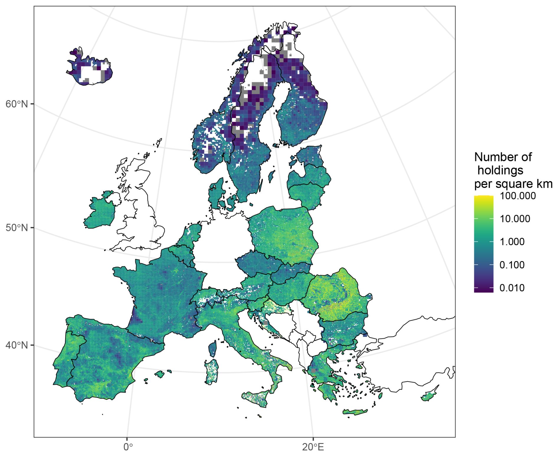
Figure 3 The number of farms per square km across Europe in 2020. Note: as a result of some lower-resolution grid cells, there are situations where grid cells overlap borders to non-EU countries; an example is the grid cells that overlap between Ireland and Northern Ireland. However, all grid cells relate to data from the survey countries. Alternatively, clipping the grids to survey country borders and coastlines would remove this undesirable effect.

On the other hand, high farm concentration might also be directly related to the widespread existence of small-scale subsistence⁶ or semi-subsistence patterns. Most of these farms are located in Eastern countries, notably Romania, Poland, and Bulgaria, but high numbers also occur in southern European countries such as Greece, Italy, and Portugal (Davidova et al., 2009; Davidova, 2014; Kostov and Lingard, 2002). Although Romania and Poland had the majority of subsistence farms in 2020, both countries have a history of mainly family farms, which in many cases were partitioned among the heirs, creating many smaller farms.

The grid cell sizes are generally too small to be seen in this figure, except for Scandinavia and Iceland. Greater detail will be more easily visualized in some of the zoomed-in maps provided in the later subsections, as well as directly from the interactive map viewer as described in Sect. 4.

3.1.2 C18 – share of arable land

Arable land includes temporary crops that do not last more than one season, such as cereals, fodder crops, dry pulses, root crops, or industrial crops (Eurostat, 2020). Figure 4 maps the share of arable land in the UAA and highlights divergent geographical patterns. High shares are particularly evident in large areas of Scandinavia, south and east of the Carpathian mountains in Romania, and in several other regions such as the Paris Basin and South Aquitaine in France, Castile-Leon in Spain, the Po Valley in Italy, and the regions of Poludniowy and Zachodni in Poland. This observation coincides with the findings of Ballot et al. (2023), demonstrating that the crop sequence types are concentrated in specific parts of Europe. Substantially lower shares of arable land often arise from natural constraints, soil characteristics, or favorable conditions to grow perennial crops (e.g., fruit trees, olive trees, or grapes for wine). For instance, grassland is predominant in Ireland due to the mild maritime climate conditions, while permanent crops dominate in the European Mediterranean region such as in the southeast of France, Spain, Italy, Portugal, and Greece. This differentiation may be determined mainly by factors of physical location, natural constraints, and climate change, which impact the choice of crop production, compared to cultural traditions and political choices (Schneider et al., 2023; Ronchetti et al., 2024).

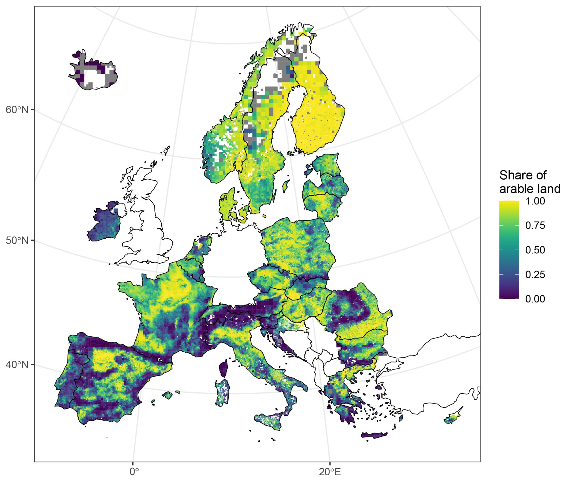
Figure 4 The share of arable land in the UAA across Europe in 2020. Note: as a result of some lower-resolution grid cells, there are situations where grid cells overlap borders to non-EU countries; an example is the grid cells that overlap between Ireland and Northern Ireland. However, all grid cells relate to data from the survey countries. Alternatively, clipping the grids to survey country borders and coastlines would remove this undesirable effect.

3.1.3 C21 – livestock density index

The livestock density index (LDI) provides an indication of the pressure of land-based animal farming on the environment, such as nutrient surpluses. The index is expressed as the number of LSU per hectare of UAA. A single livestock unit is a reference unit that facilitates the aggregation of livestock from various species and ages according to an agreed standard through the use of specific coefficients,⁷ established initially based on the nutritional or feed requirements of each type of animal (European Commission, 2024a). Figure 5 illustrates the concentration of high index values in Europe.

The map has a cutoff point at the animal stock rate of 10 to better highlight the patterns and to avoid displaying those that contain mainly specialized livestock and indoor farming with almost no UAA. Consistent with the findings of Tattari et al. (2012), LDI is more pronounced in the heterogeneous landscapes of Finland and Sweden, where the spatial variation in arable land (e.g., temporary grasslands) is high.

Values above 3–4 LSU per hectare tend to be indications that animals in these regions depend on other feedstuffs rather than grass, maize, harvested greens or cereals (Green et al., 2016). This pattern becomes even clearer if compared with Fig. 4, which shows that many of the regions with high LDI values are also regions with a high share of arable land, most notably Brittany in France, North Brabant in the Netherlands, West Flanders in Belgium, and Lombardy in Italy. Although some of the arable land can be used as temporary grazing land or self-produced feed, it is not sufficient to support livestock in these regions. Wang et al. (2018) undertook a cross-country study showing that variations in livestock density were associated with changes in the net import of soybeans and maize. The density of livestock increased even faster in the main soybean and maize importing countries, such as France, Spain, Germany, and the Netherlands, which have experienced a strong increase in LSU/ha in recent decades. For example, the volume of imported protein for livestock production in France increased from 0.2×10⁶ t in 1961 to 5.24×10⁶ t in 2003 (Chatzimpiros and Barles, 2010). High livestock densities and the import of feed protein drive land-use changes and generate negative externalities due to the physical flows of nitrogen (Burke et al., 2009; Chatzimpiros and Barles, 2010). Other studies revealed that the density of livestock affects the function and structure of the ecosystem, such as species composition, loss of biodiversity, and the alteration in the nitrogen and phosphorus cycles (Kasiske et al., 2023; Kok et al., 2020).

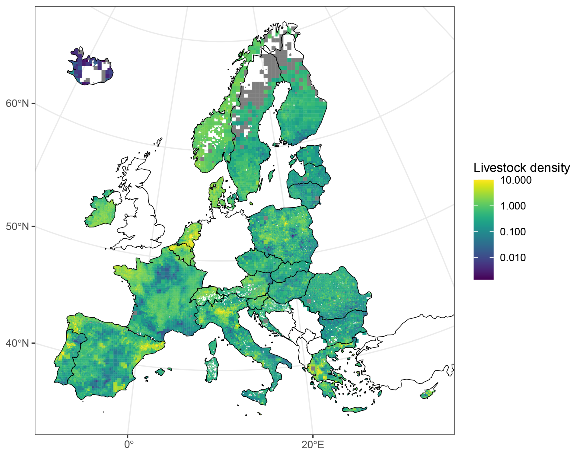
Figure 5 The livestock density index across Europe in 2020. Note: as a result of some lower-resolution grid cells, there are situations where grid cells overlap borders to non-EU countries; an example is the grid cells that overlap between Ireland and Northern Ireland. However, all grid cells relate to data from the survey countries. Alternatively, clipping the grids to survey country borders and coastlines would remove this undesirable effect.

3.1.4 C22 – family farming

Family farms have been the backbone of EU agriculture for centuries. An indication of their importance is that family farms accounted for approximately 90 % of the 9 million farms in 2020 (European Commission, 2023d). Although family farms constitute the most predominant farming business model, they operate at very different scales in the EU ranging from small semi-subsistence farms to much larger farms that are managed by the family and passed down through generations.

There is no formal agreed definition of a family farm in the literature, yet the most common element used to distinguish between family and non-family farms is the labor criterion, which implies that the majority of the labor force is supplied by the family (Calus and Huylenbroeck, 2010; Djurfeldt, 1996; Graeub et al., 2016; Toader and Roman, 2015; van Vliet et al., 2015). Based on the statistical definition of FAO (2014), we use the term family farm hereafter to refer to any farm under family management (i.e., sole holder holdings) where 50 % or more labor was provided by family workers (European Commission, 2023d).

With respect to corporate farming, no information on family workers was collected in the IFS as it is presumed that group holdings and legal entities do not have family workers, and thus by default, they are not family farms. In reality, this may not necessarily be the case, as a family-run business – where family workers make up 50 % or more – can choose a legal entity for legal and economic reasons.⁸ Figure 6 maps the spatial distribution of family farms in 2020 across Europe. Although the share of family farms is evenly distributed and substantially high in most countries, the proportion of family labor is particularly low in France and Estonia. This could be explained by the fact that there is a high proportion of large incorporated farms that operate mainly on the basis of wage labor. Moreover, the share of non-family labor in terms of employed persons is almost 10 times higher in France (56 %) and Estonia (45 %) than in Poland (5 %) (Eurostat, 2024a).

In addition, we observe a heterogeneous pattern in Denmark, Belgium, Finland, Czechia, Slovakia, Bulgaria, Spain, and Portugal where the distribution of the family farm is more dispersed and the share is on average 5 % to 15 % lower. In contrast, the proportion of family farms is over 90 % and is mostly homogeneous in Lithuania, Latvia, Poland, Romania, Switzerland, Greece, Croatia, and Slovenia.

Although the variation in the share of family farms is less pronounced in most countries, there are considerable local and regional divergences within certain countries and regions such as between the north and south of France, Spain, and Portugal. For example, there is a relatively high density of family farms in the northwestern part of Portugal in the Terras de Trás-os-Montes region, while a much lower concentration is found in the Alentejo region. With its vast plains, fertile soils and good environmental conditions, Alentejo is the main agricultural region in Portugal that is known for its production of cereals, olive oil, wine, and cork. In the last decade, the region has witnessed the continuous disappearance of farms and, at the same time, rapid agricultural intensification leading to concentration in large agricultural companies. The new agrarian business model in this region is mainly based on intensive monoculture encompassing the usage of modern irrigation technology and relying on seasonal foreign workers (Almeida, 2020; Cardoso, 2018).

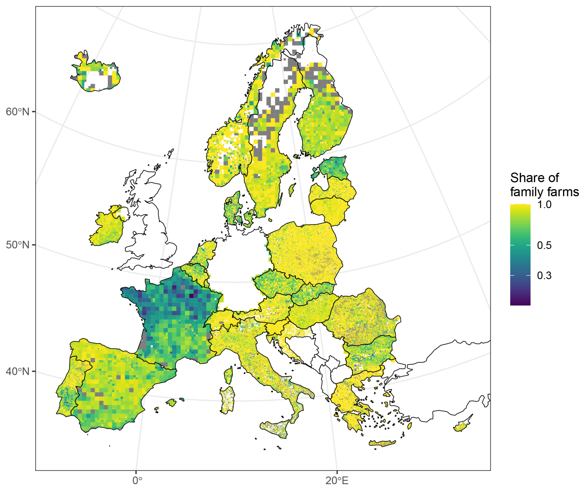
Figure 6 The share of family farms across Europe in 2020. Note: as a result of some lower-resolution grid cells, there are situations where grid cells overlap borders to non-EU countries; an example is the grid cells that overlap between Ireland and Northern Ireland. However, all grid cells relate to data from the survey countries. Alternatively, clipping the grids to survey country borders and coastlines would remove this undesirable effect.

3.1.5 C23 – age structure of farmers

The aging crisis in agriculture poses a considerable threat to global food security, and it remains a major challenge in rural areas of Europe. The CAP is dedicating specific policy measures to support generational renewal to secure the transfer of farms from one generation to the next. We emphasize this topic in theme 2 on farmer demographics.

Figure 7 depicts the current situation of an aging crisis by mapping the distribution of the average age of farm managers in Europe in 2020. The map highlights striking patterns for this indicator not only between and within countries, but also within specific regions. The average age of farm managers is typically higher in southern Europe than in central and northern Europe, and it is higher in northern Europe compared to central Europe. The youngest farm managers are found in a “belt” that runs from France through Switzerland, Austria, Czechia, Slovakia, and Poland. We can observe particularly high ages in some regions of Spain and Portugal, while Bulgaria and the northern part of Greece have younger managers than the rest of these regions. Moreover, Norway, Finland, and Estonia have older farmers than other northern countries. Yet, there is also significant differentiation in the age groups of farm managers within certain regions, such as Galicia and Catalonia in Spain, Veneto in Italy, or Plovdiv in Bulgaria (see Fig. 10d in Sect. 3.2 for further illustrations and explanations).

Analyzing the aging crisis of farmers in Europe is a daunting challenge due to the multitude of interacting factors. Farm entrepreneurship can be determined by cultural and political dimensions, where varying practices or traditions can occur in different regions with respect to how farmers are granted the responsibility to manage the farm. While in some parts of Europe farms will typically change the farm manager when the responsibility for the daily farming duties is altered, in other regions, a farm manager might keep the administrative responsibility much longer, even if another family or non-family member is actually responsible for the main agricultural operations. These divergences in the uptake of the farm management role can be explained by cultural traditions, legal aspects that create economic benefits and tax reductions, or the type of farming (i.e., a family farm or a more industrial type of farming). Nevertheless, the spatial variations in the aging pattern still point towards structural differences in management, and they can help to identify geographical areas that have a high risk of farm disappearance. A report on farming in Romania has indicated that older farmers generally manage smaller farms in comparison to younger ones, and the percentage of succession of ownership within the family was only 26.5 % in 2010 (Baker-Smith, 2016). By cross-correlating different management characteristics (e.g., age, gender, vocational training, management practices, and skills) on a grid cell basis, we can better understand the policies needed to keep or modify the current situation.

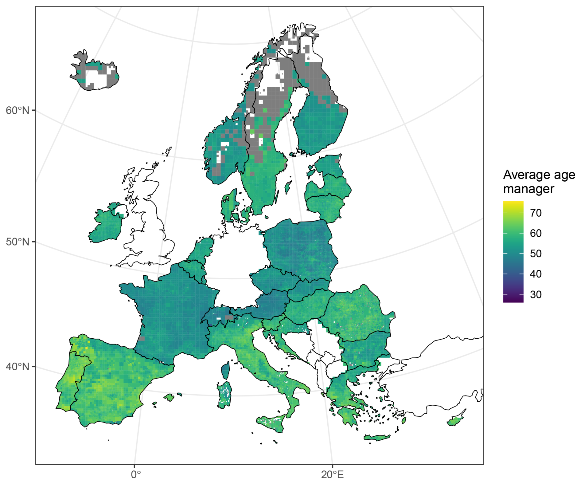
Figure 7 The average age of farm managers across Europe in 2020. Note: as a result of some lower-resolution grid cells, there are situations where grid cells overlap borders to non-EU countries; an example is the grid cells that overlap between Ireland and Northern Ireland. However, all grid cells relate to data from the survey countries. Alternatively, clipping the grids to survey country borders and coastlines would remove this undesirable effect.

3.1.6 Female managers

Although gender mainstreaming has become an important principle within the CAP, due to the poor implementation and weak commitments, several EU institutions and studies have criticized the lack of achievement of gender balance in agriculture (ECA, 2021; EPRS, 2022; Prügl, 2010; Shortall and Marangudakis, 2022, 2024). Moreover, there was a clear shortfall in specific measures to address gender mainstreaming in the CAP for the period 2014 to 2022 as no clear objective or statement on gender equality was included in the EU Regulation to support rural development (European Commission, 2013) and, additionally, no contextual indicator on the gender gap in farming was established. Nevertheless, current CAP strategic plans (2023–2027) are required to include a gender equality approach by setting specific targets at the national level to improve the participation of women in agriculture.

At a first glance, the gender gap in agricultural entrepreneurship seems to be unevenly distributed across Europe in 2020 (see Fig. 8). The map indicates the opposite picture of what one would initially expect. While Finland, Sweden, and the Netherlands are well-known to rank high in the overall gender equality indicators established by various international organizations (European Institute for Gender Equality, 2023; World Economic Forum, 2024; Eurostat, 2024b), Fig. 8 highlights a clear pattern of gender gap, with women uniformly underrepresented in agricultural entrepreneurship in almost all regions in these countries. In contrast, the share of women who are operating as a farm manager is, on average, higher in two Baltic countries (Latvia, Lithuania), Austria, Poland, Romania and parts of Italy, Greece and Spain.

Zooming into Spain, we can observe that the gender gap is much less pronounced in Galicia compared to other regions of Spain. Galician rural areas have preserved small-holding cultural practices based on polyculture and family farming instead of heading for exclusively industrial agricultural development. Moreover, Galicia has a long tradition of small-scale cooperatives representing one of the most important cooperative sectors in Spain, accounting for 25 % of agricultural enterprises in this region (Ferrás-Sexto and O'Flanagan, 2012; Bastida et al., 2020; Fandiño et al., 2006).

Recent research has shown that there is a positive association between cooperatives and female entrepreneurship (Bastida et al., 2020; Henry et al., 2016). The role of women in cooperatives is determined by legal, cultural, and economic determinants, and it seems that this economic model is suitable for the work and lifestyle of women in such regions (Bastida et al., 2020). Studies on social entrepreneurship have found that women prefer this corporate model over the more traditional ones, because cooperative principles, such as solidarity, fair and democratic management, and social responsiveness, fit well with their individual preferences and their perception to pursue personal and professional development (Senent, 2008; Senent Vidal, 2011; Ribas Bonet, 2005; Vidal, 2014). Moreover, women perceive cooperatives to be less risky due to profit and cost sharing (Bastida et al., 2020; Salvador et al., 2016).

These wide-ranging factors might partially explain the high share of women involved in farm management in Galicia, but further research is needed to better understand the interaction of exogenous and endogenous factors in a local context across Europe. Displaying the relationship between two or more variables in bivariate and trivariate maps might be useful for identifying common patterns in a European context.

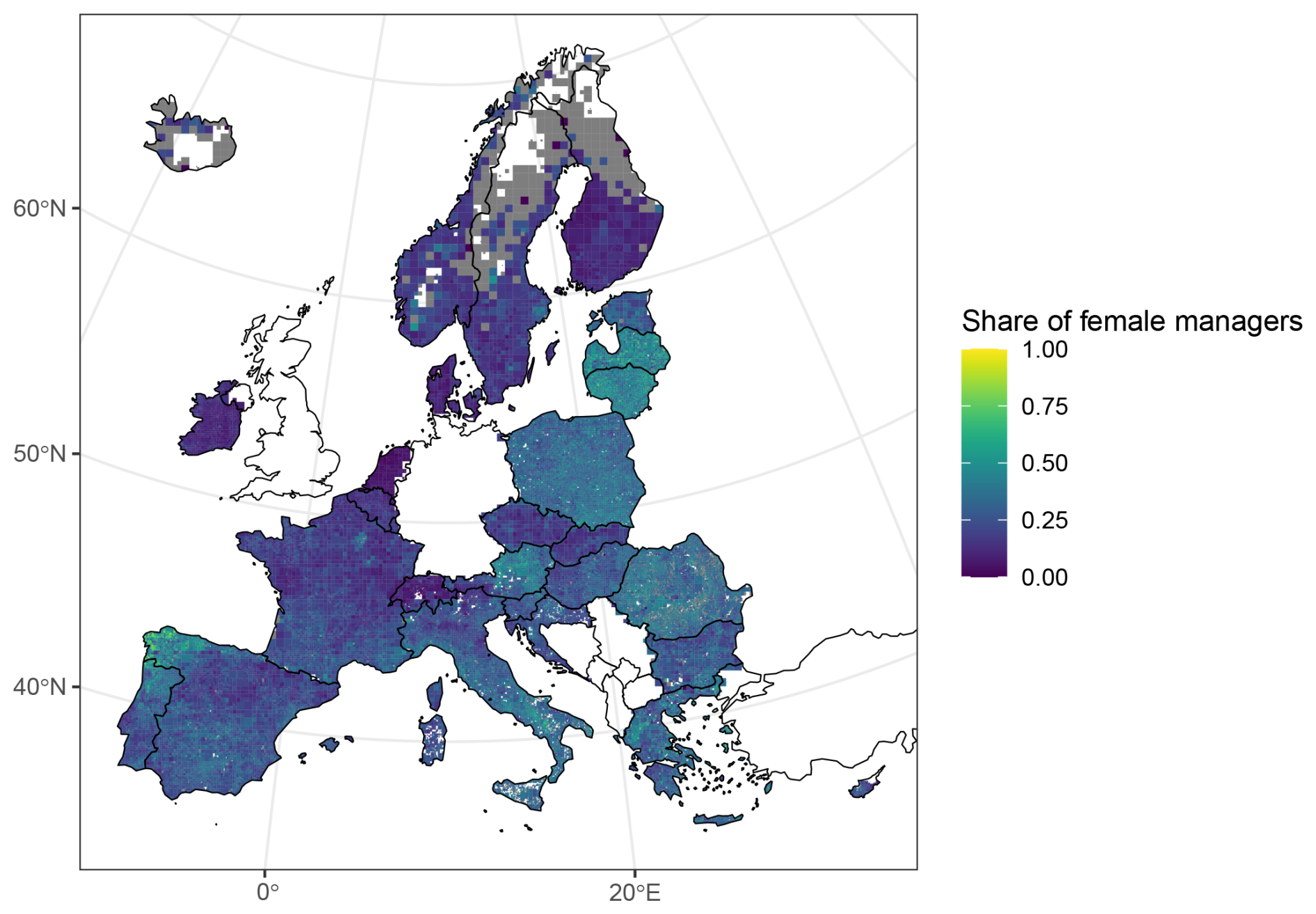
Figure 8 The share of female managers across Europe in 2020. Note: as a result of some lower-resolution grid cells, there are situations where grid cells overlap borders to non-EU countries; an example is the grid cells that overlap between Ireland and Northern Ireland. However, all grid cells relate to data from the survey countries. Alternatively, clipping the grids to survey country borders and coastlines would remove this undesirable effect.

3.1.7 C19 – organic farming

Organic farming is an agricultural production method that aims to use natural substances and processes. It tends to limit the environmental impact of agriculture through a more responsible use of natural resources, allowing the maintenance of biodiversity and water quality, the enhancement of soil fertility, and the preservation of the regional ecological balance (European Commission, 2024b).

Expanding agricultural land in organic farming is at the heart of the Farm-to-Fork strategy under the European Green Deal. The European Commission launched an organic action plan in March 2021 to increase organic agricultural land, which should represent at least 25 % of agricultural land in the EU by 2030 (European Commission, 2021). In 2020, organic agriculture covered an estimated 14.7×10⁶ ha of agricultural land in the EU, which is equivalent to 9.12 %⁹ of total UAA (Eurostat, 2024).

As part of the third theme on agricultural production methods, Fig. 9 shows the spatial distribution of organic farming in 2020, which is the contextual indicator C19 of the CAP. Although it is widely recognized that the diffusion of organic farming is substantially higher in certain countries (Austria, Czechia, Estonia, Finland, France, Italy, Latvia, Spain, Switzerland, and Sweden), the map additionally reveals specific organic farming hotspots with common patterns. These include the border triangle of Italy–Croatia–Slovenia, the low mountain range in Central Europe (Bohemian Forest), the main islands in Estonia, and the mountain ranges of Madonie and Monti Nebrodi in the northeast of Sicily, covering mainly large areas of pasture, meadow, and grasslands. This pattern is particularly evident in the Salzburg region in Austria, which represents the highest share of organic farming (52 %) in Europe, where extensive grasslands account for almost 97 % of the organic area.¹⁰

Moreover, the map indicates that organic farming might be linked to livestock farming in areas with a high share of organic forage legumes, cereals for feed, and temporary and permanent grasslands. Grassland and harvested greens (e.g., forage legumes, perennial clover, grass plants) from arable land play a crucial role in organic livestock farming because they build up soil fertility with minimal use of non-renewable resources, in addition to providing a valuable and cheap feed supply for livestock products (Huyghe et al., 2014; Fraser et al., 2022; Younie and Baars, 2019).

In addition, we can observe higher organic farming diversity in Puglia, Calabria, and Sicily in the south of Italy and areas in Andalusia and the region of Murcia in the south of Spain where organic permanent grassland dominates in highland areas and organic permanent crops, pulses, and cereals for grain production are more pronounced in valleys and lowlands. However, we did not observe this pattern in similar regions in Greece, Bulgaria, or Romania. In addition to the topographic and climatic factors that favor good conditions for organic agriculture production, there may be other intrinsic and extrinsic factors that will play a key role in the diffusion of more sustainable farming practices.

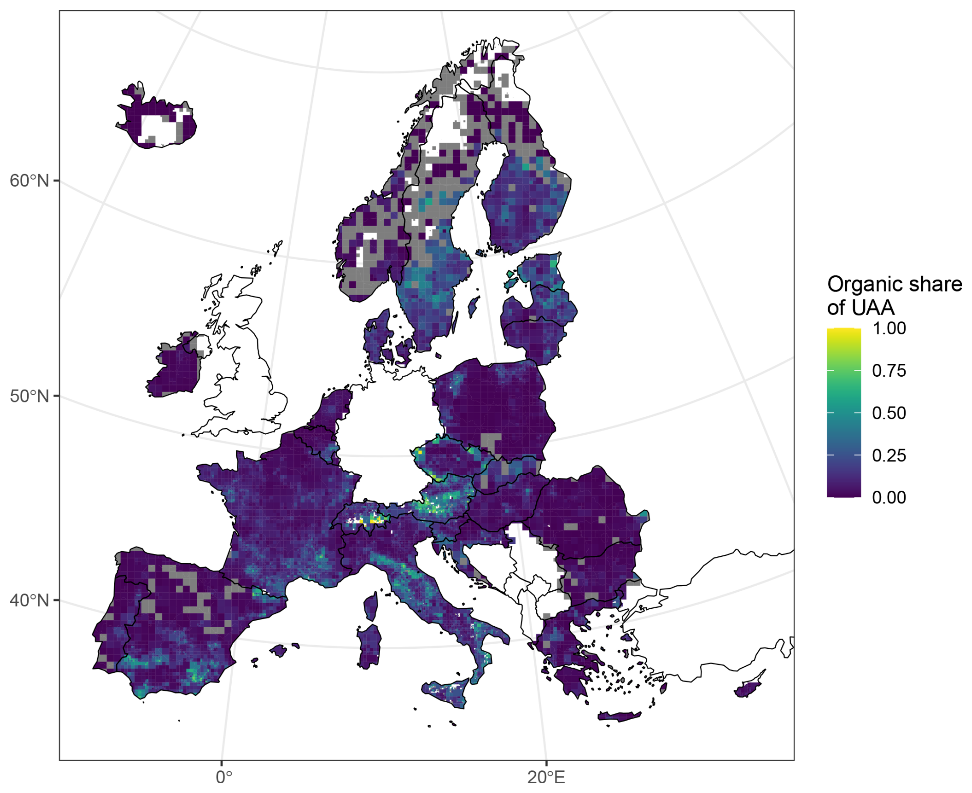
Figure 9 Share of area under organic farming across Europe in 2020 (C19). Note: as a result of some lower-resolution grid cells, there are situations where grid cells overlap borders to non-EU countries; an example is the grid cells that overlap between Ireland and Northern Ireland. However, all grid cells relate to data from the survey countries. Alternatively, clipping the grids to survey country borders and coastlines would remove this undesirable effect.

3.2 Divergent patterns within NUTS 2 regions

One of the advantages of a multigridded approach is the ability to provide the data at a much higher resolution than the NUTS 2 region, which is the smallest administrative zone at which aggregated data are currently released by Eurostat. However, some of these regions are quite large, so the finer spatial variations in the data are lost at this scale.

To demonstrate that multi-resolution grid data provide greater insight into the spatial variations within the broader region, Fig. 10 displays the deviations between the grid values and the regional summary statistics for different agricultural indicators in 2020 published by Eurostat¹¹ for four NUTS 2 regions, which are Helsinki-Finland (Fig. 10a), Pays de Loire-France (Fig. 10b), Catalonia-Spain (Fig. 10c), and Yuzhen-Bulgaria (Fig. 10d).

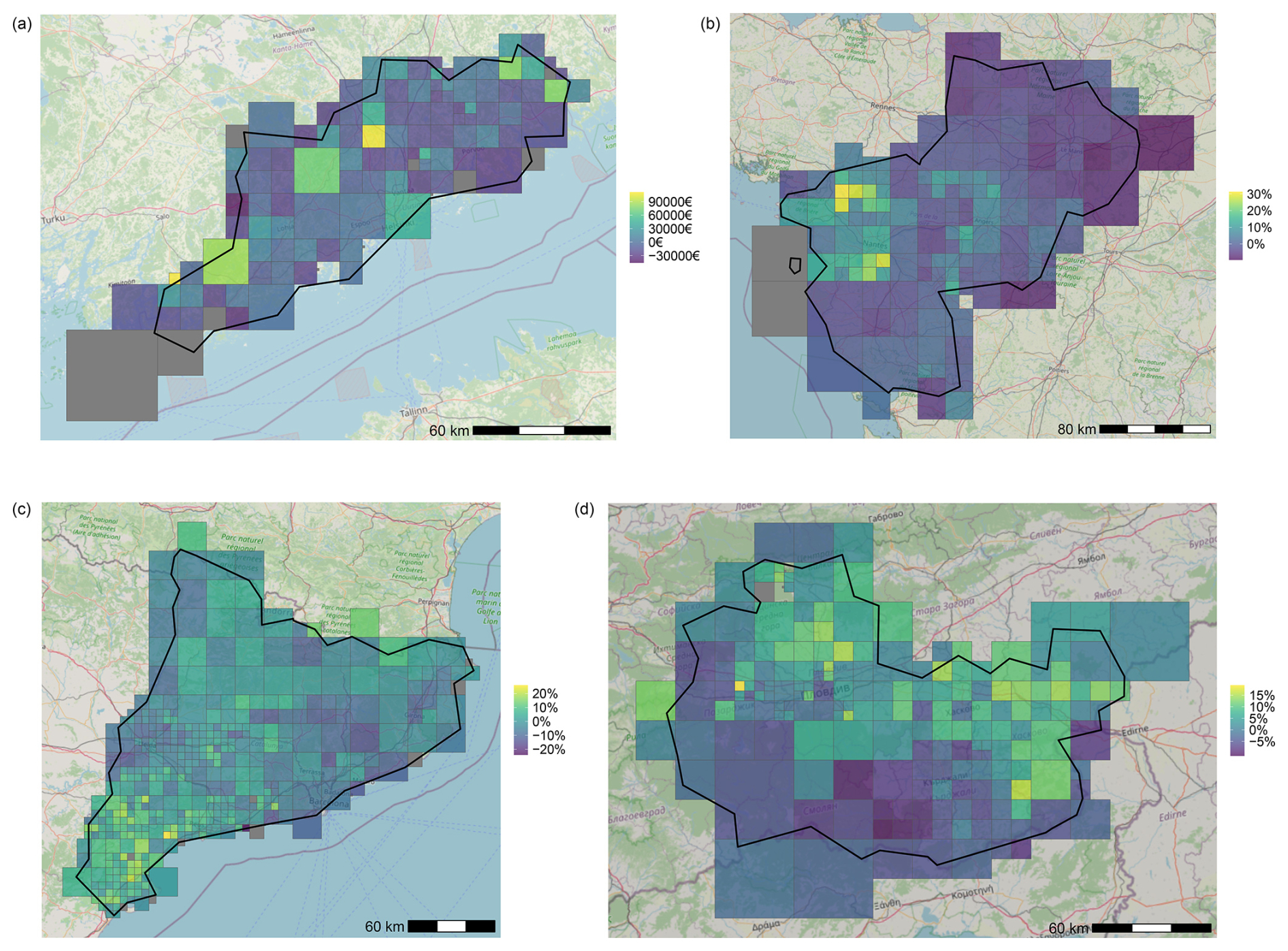
Figure 10 Absolute differences between the multi-resolution gridded data and the NUTS 2 values for the 2020 agricultural census.

Our analysis reveals that there are large discrepancies within the region ranging from more dispersed local concentrated areas in the region of Helsinki (FI1B) to the appearance of distinct spatial clusters in the region of Pays de Loire (FRG0), Catalonia (ES51), and Yuzhen (BG42). For example, the concentration of young farmers tends to be higher in specific areas in the north of Plodiv, the second largest city in Bulgaria, and in the Haskovo province, which neighbors Greece and Türkiye, varying between 20 % and 30 % compared to the average regional value of 14 % in the Yuzhen region.

3.3 Linking measures from contextual indicators

Side-by-side univariate maps may initially be useful for identifying common characteristics; however, they do not reveal relationships and patterns between two different types of data. To further explore the potential of the data, we have established the statistical association between two variables from two distinct context indicators through a bivariate choropleth map.

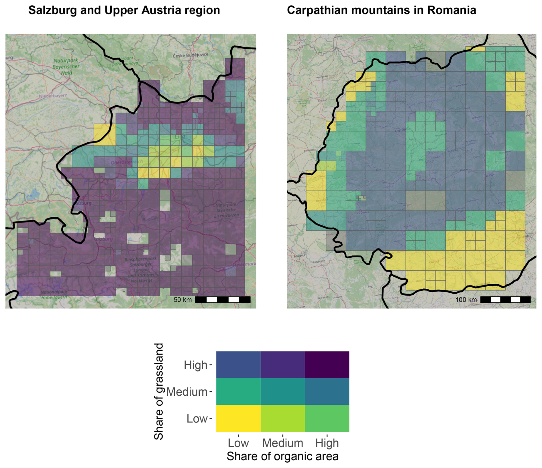
Figure 11 Bivariate choropleth map of the proportion of organic area and permanent grassland.

To illustrate an example, we link the data from the share of permanent grasslands (C18) with the share of organic area (C19) and display two contrasting outcomes in Fig. 11. The grid cells use color to show the proportion of agricultural holdings with a high share of organic farming areas and permanent grasslands, as highlighted in the legend. For example, a dark purple cell indicates a high percentage of organic areas and permanent grasslands, while a blue cell shows most farms with a low proportion of organic areas, but a high share of permanent grasslands.

As explained in Sect. 3.1.7, we observe a strong pattern in the Salzburg region in Austria where the share of organic area and extensive grasslands is substantially high. Although both regions share similar topographic conditions, we do not observe the same pattern for the Carpathian mountains in Romania, where non-organic grasslands dominate the farming landscape. The Pearson correlation between both variables is 0.24 for all European countries, 0.72 for the selected area in Austria, and −0.16 for the selected area in Romania (see Table A2 and Fig. A1 in the Appendix for a quantitative assessment by country).

It seems that organic farming occurs in some parts of Europe in less favored areas, where economic incentives for conversion to organic farming are less stringent and the economic loss of production is relatively small (Gabriel et al., 2009). However, our exploratory analysis highlights that environmental factors are not the only ones that could play a vital role in the conversion to organic farming. These divergent outcomes hint at the fact that the uptake of organic agriculture could be influenced by a multitude of intervening factors at the micro and macro level (Lampach et al., 2020). To better understand the key drivers that explain the spatial distribution of organic farms, it would be beneficial to analyze the size of the farm and the use of farmland (Gabriel et al., 2009; Parré et al., 2024), the establishment and maintenance of market access, such as proximity to urban centers with high population densities (Allaire et al., 2015), location factors and agglomeration effects (Schmidtner et al., 2012), imitation and neighborhood effects (Boncinelli et al., 2016; Bjørkhaug and Blekesaune, 2013; Zollet and Maharjan, 2021; Van et al., 2023), social-cultural effects (Ilbery and Maye, 2011), and non-economic factors such as personal motivation, attitude towards the environment, and healthy lifestyles (Cranfield et al., 2010; Blaće et al., 2020), which requires the use of additional input datasets.

4 Interactive map viewer

To allow users to interact with the rich content of the data, we use an interactive mapping application that has been developed by GISCO (2024) and Gaffuri and Davies (2024) to visualize the grid layers in a web browser. The mapping tool is based on a JavaScript library that contains a large variety of features, such as zooming, displaying city names and boundaries, and different cartographic styles. The gridded data from the different layers are available at https://doi.org/10.5281/zenodo.14852709 (Eurostat, 2025) and the viewer is publicly accessible from the Eurostat Experimental Statistics web page (https://ec.europa.eu/assets/estat/E/E4/gisco/farmstatistics/index.html).

In the viewer, users can select specific contextual indicators from the drop-down box located in the upper left corner of the map. Figure 12 provides a screenshot of the web-based interactive mapping application. By zooming in and out, users can hover over the grid cells to extract detailed information about the indicators at a specific geographical location.

Users might face difficulties in the interpretation of data in a multi-resolution grid format due to the presence of varying grid sizes in a specific area. For clarification, the size of the grid provides information on the density of farms located in a cell and structural differences are immediately visible. Although a smaller grid cell at a lower level of resolution contains a high density of individual units, large cells represent a limited number of agricultural holdings.

In addition, the color scheme, which ranges from light yellow to dark blue, represents the magnitude of the indicator. The color scheme has been adjusted for each measure, and the range varies according to the chosen unit of the respective variable (see Table 2 in Sect. 2.1). Users should also be aware of the relevant information about each indicator and variable that can affect how the maps could be interpreted. This information is provided in Table A1 in the Appendix.

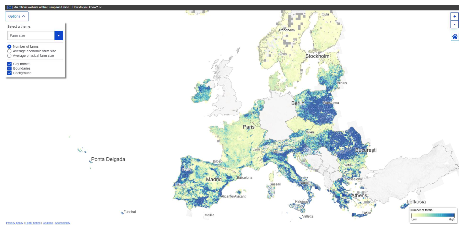
Figure 12 An interactive map to visualize the grid layers of the context indicators.

5 Code and data availability

The code for creating the multi-resolution gridded data is available as an R package called MRG from Comprehensive R Archive Network (https://doi.org/10.32614/CRAN.package.MRG, Skøien and Lampach, 2025). The data described in this manuscript can be accessed at https://doi.org/10.5281/zenodo.14852709 (Eurostat, 2025). Eurostat and MS coordinate the organization of agricultural surveys and censuses in the IFS Working Group. The release of geospatial data was approved by all countries except Germany. Eurostat and Germany are working together to overcome secondary confidentiality concerns and hope to release German IFS data within these EU spatial data layers as soon as possible.

6 Conclusions

This paper provides an overview of newly available data from the 2020 European agricultural census in the form of key context indicators that are used for monitoring the CAP as well as other contextual variables of interest related to the European agricultural sector. The data are provided as hierarchical multi-resolution grids varying from 1 to 40 km in size, which ensure that any legal statistical disclosure requirements have been fully met. The spatial distributions of a selected set of indicators were presented here although users can view and download the complete set from the GISCO viewer as described in Sect. 4.

In addition to the improved monitoring potential for the CAP (and other EU Green Deal policies), the multi-resolution gridded agricultural census data can be used to compare various aspects of the agricultural sector in different countries across Europe for gaining insights into regional agricultural development. A greater understanding of the spatially explicit patterns observed within an individual country could also be undertaken. Studies on drivers of certain types of agricultural practices such as organic farming would be possible at a higher resolution than previously undertaken, while detailed analyses of farmer demographics and high-resolution changes in the farming sector over time are now possible. Combinations of variables would also allow for the development of detailed farm typologies, while the data could be useful inputs for modeling the impacts of agriculture in areas such as the environment and biodiversity, among others. We envisage that such spatially explicit high-resolution information on the agricultural sector in Europe will open up whole new avenues of research and innovation, as has already been observed when public sector data have been openly shared (Coyle et al., 2020).

Future developments include the release of other variables of interest from the 2020 European agricultural census as well as plans for processing variables from previous censuses and surveys, e.g., the 2010 agricultural census and various agricultural surveys that took place between 2010 and 2023. Attention will be paid to methods for aligning the temporal multi-resolution grids for studies that will specifically consider changes over time.

Appendix A

(Eurostat, 2020)(Eurostat, 2020)

Table A1 Caveats related to the multi-resolution gridded data.

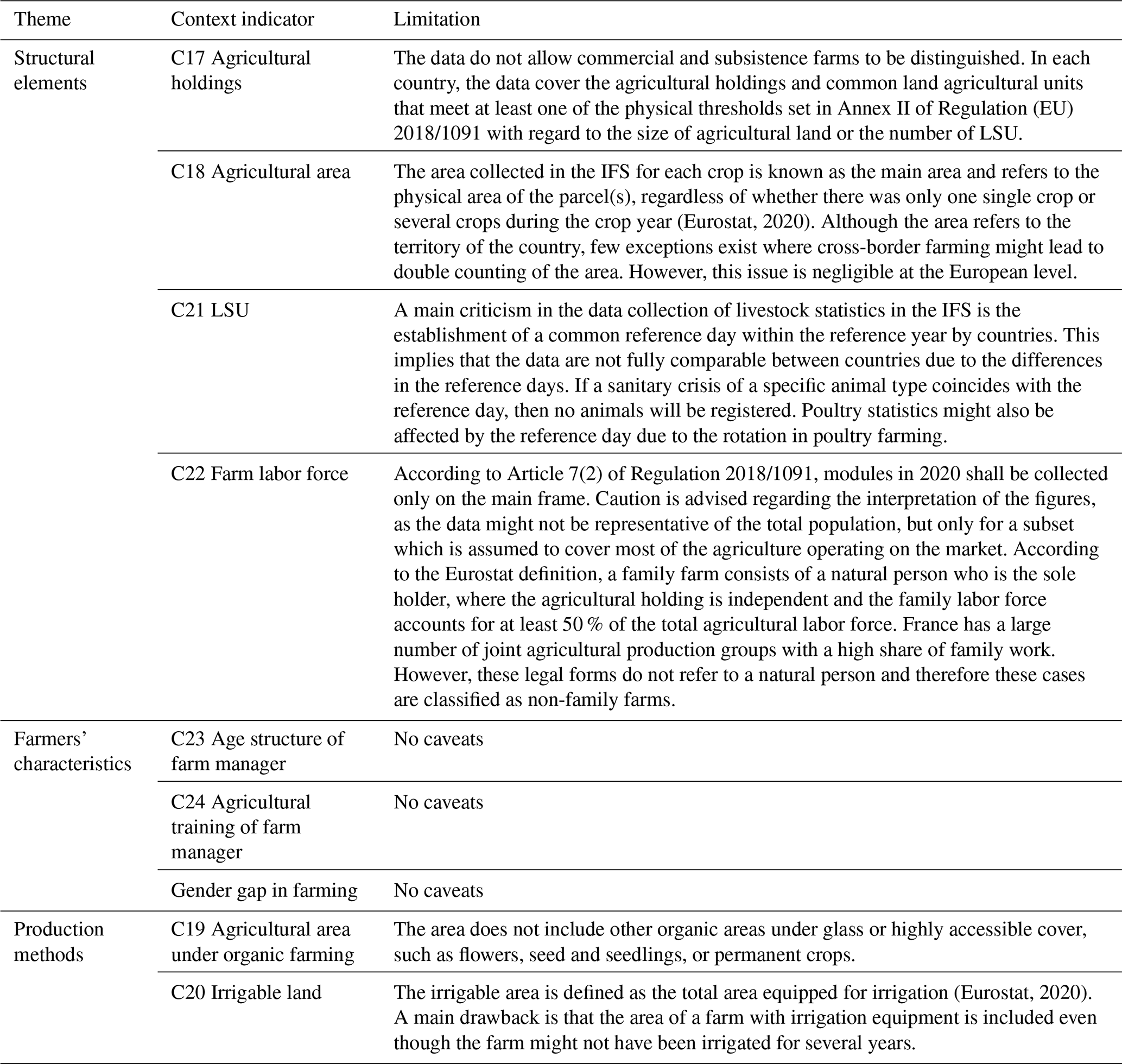
Note: further information can be found in the metadata of the IFS survey (https://ec.europa.eu/eurostat/cache/metadata/en/ef_sims.htm, last access: 19 May 2025).

Table A2 Statistical association between grasslands and organic area by country.

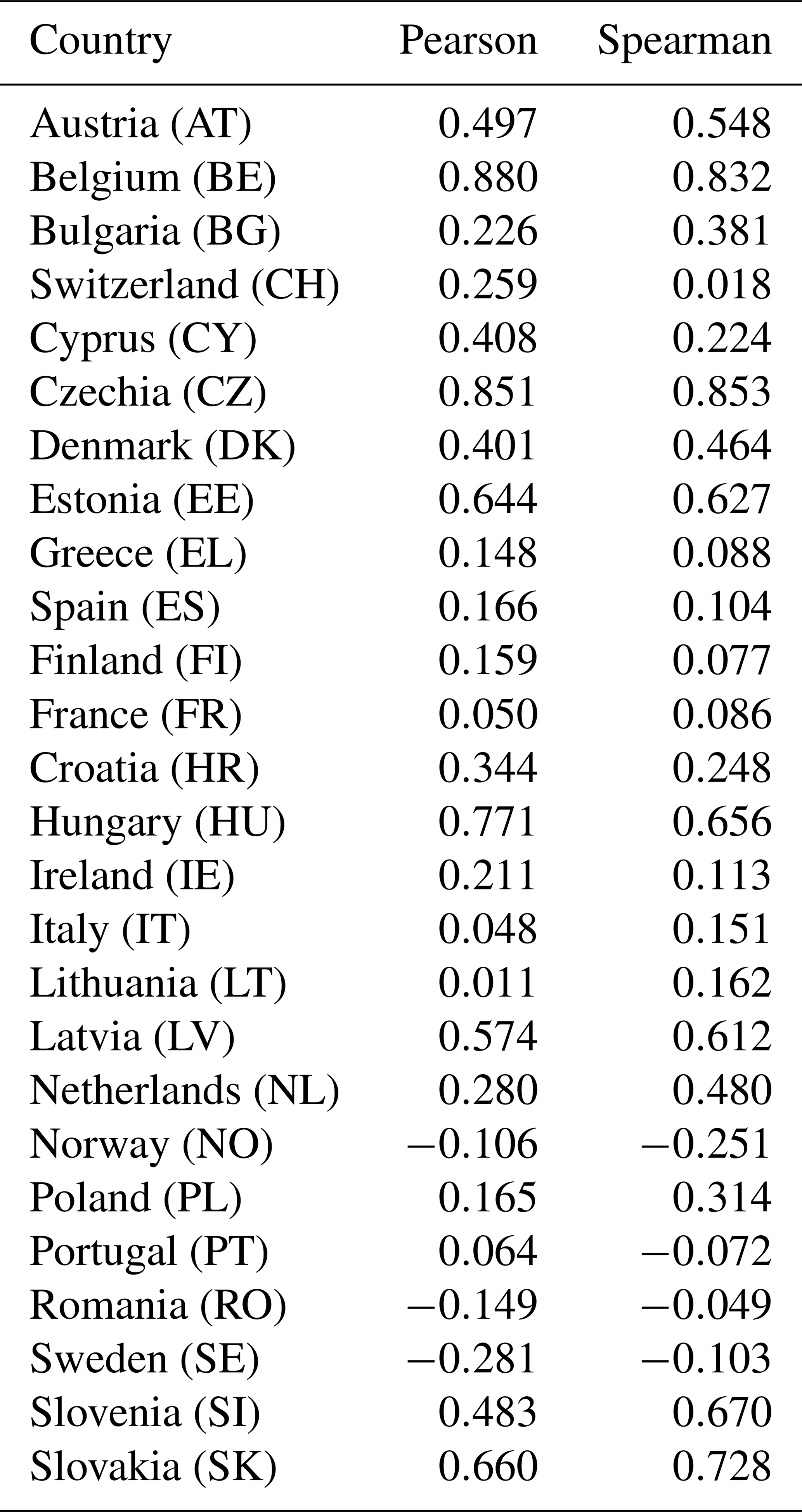
Note: Luxembourg is excluded due to insufficient information.

According to Skøien et al. (2025), the list below and Fig. A2 explains the iterative process of producing a nested structure of multi-hierarchical grids satisfying a set of confidentiality rules and quality requirements. We denote the resolution level k∈K with $K=\mathit{\{}{k}_{\mathrm{0}},k_{\mathrm{1}},\mathrm{\dots },k_m\mathit{\}}$ where k₀ is the highest resolution (1 km) and k_m the lowest resolution. The first iteration is i₁, the possible aggregation from k₀ to k₁, and continues until it reaches the maximum level k_m ($i\in \mathit{\{}{i}_{\mathrm{1}},\mathrm{\dots },i_m\mathit{\}}$). For each iteration, the following steps are evaluated (it is sufficient to pass one of the dominance rules):

1. Threshold rule:

   If the aggregated extrapolated number of farms in grid cell l (W_l) for resolution k_i is less than 10 (W_l<10 with $W_l={\sum }_{j=\mathrm{1}}^{n_l}{w}_j$; n_l is the number of records in l).

2. Dominance rule I:

   This rule is satisfied if, after ordering the variable of interest in descending order, the sum of the weights ($w_{j{max}_{\mathrm{1}}}$ and $w_{j{max}_{\mathrm{2}}}$) of the two highest values ($x_{j{max}_{\mathrm{1}}}$ and $x_{j{max}_{\mathrm{2}}}$) is greater than 2 ($w_{j{max}_{\mathrm{1}}}+w_{j{max}_{\mathrm{2}}}>\mathrm{2}$). (The weights in IFS are rounded before this step, so greater than 2 means at least 3.)

3. Dominance rule II:

   If the weighted sum of the two potential dominant contributors are less than or equal to 85 % of the extrapolated aggregated value of the grid cell ($w_{j{max}_{\mathrm{2}}}\times x_{j{max}_{\mathrm{2}}}+w_{j{max}_{\mathrm{1}}}\times x_{j{max}_{\mathrm{1}}}\le \mathrm{0.85}\times X$), then the confidentiality rules are satisfied.

4. Reliability of the results:

   The indicator is reliable if the estimated coefficient of variation for the grid cell at k_i is less than 35 %, (will be disseminated with a warning if above 25 %);

5. Repeat:

   If not passing the threshold rule, the quality rule (if applicable), or one of the dominance rules, the grid cell will be aggregated with neighboring grid cells, and the steps above will be repeated (unless the value is below the suppression limit).

After the last iteration, and as a measure to add further perturbation to the disclosed information, all nonconfidential extrapolated number of farms and extrapolated aggregated values of variables are rounded to the nearest multiple of 10.

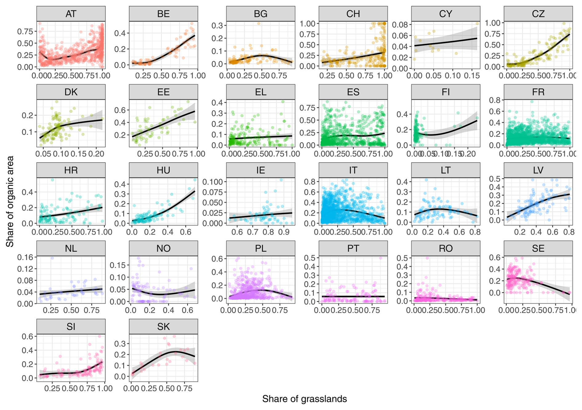
Figure A1 Relationship between grasslands and organic area by country. Note: Luxembourg is excluded due to insufficient information.

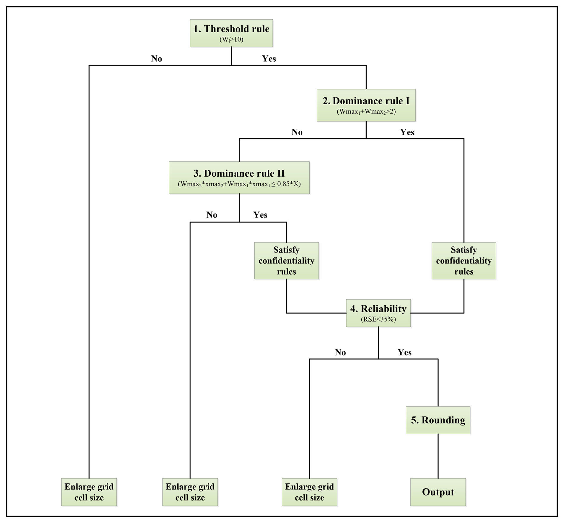
Figure A2 Iterative process to produce multi-resolution grids from Integrated Farm Statistics (IFS) data that satisfies the confidentiality rules and quality criteria. Source: Skøien et al. (2025).