PL1GD-T: a high-resolution gridded daily air temperature dataset for Poland

This paper presents a high-resolution gridded dataset of daily minimum (TN), mean (TG), and maximum (TX) near-surface air temperatures over Poland, covering the period from 1951 to 2020, with a spatial resolution of 1 km². The PL1GD-T dataset was developed using radial basis functions (RBFs), which were applied to quality-controlled observations from 347 ground weather stations at the Institute of Meteorology and Water Management – National Research Institute. TG is calculated consistently using the same formula throughout the entire period, and daily TN, TG, and TX fields are generated based on available daily records. Cross-validation methods evaluated the gridding procedure on a monthly basis. The linear RBF was selected by hold-out cross-validation (HO-CV) as the most suitable for the gridding procedure among other RBFs. The leave-one-out cross-validation (LOO-CV) was performed to ensure the ability to reproduce the original characteristics variability. The values of the scores averaged over all stations for individual months are in the range of 0.3–0.2, 0.3–0.2, and 0.1–0.2 (K) for the bias; in the range of 1.23–1.46, 0.69–0.92, and 0.84–0.99 (K) for the root-mean-squared difference (RMSD); and in range of 0.91–0.97, 0.98–0.99, and 0.98–0.99 for the correlation for TN, TG, and TX, respectively. The RMSD is clearly altitude-dependent, increasing from lowland to mountainous regions. The dataset's scope and resolution allowed for the robust estimation of local climate variability characteristics and observed trends. The availability of high-resolution datasets in both spatial and temporal contexts is essential for climate change impact analysis on a smaller scale. This new dataset provides a quality-validated, high-resolution, and open-access dataset that could be utilised by society, administrative bodies, or research institutions for climate-related applications. The dataset is publicly available from the repository of the Institute of Meteorology and Water Management – National Research Institute at https://doi.org/10.26491/imgw_repo/PL1GD-T (Jaczewski et al., 2024).

1 Introduction

Contemporary climate change is one of the most significant issues facing civilisation. It affects societies in many ways, from direct physical impacts (droughts, floods, extreme events like tornadoes, heatwaves, and wildfires) to influencing the economies. We have no other way than to adapt, but our measures strongly depend on the quality and quantity of climate information we can acquire. Applications in research, natural resource management, and infrastructure planning typically require adequate spatial and temporal resolution (often 30 years of climate normality), and for a record of past climate change (historical time series), you need long-term climate baseline data. The applicability of such data lies in the availability of measurement data from National Meteorological and Hydrological Services (NMHS) networks and in the ability to assess climate change locally, which is more important in the context of adaptation. Climate change impact analysis requires the availability of high-resolution datasets in both spatial and temporal contexts. This is especially crucial if the study is to be performed on a smaller scale (administrative, physical–geographic). This assumption is rarely met with the stations' density operating in NMHS. Thus, there is a clear need to prepare a quality, validated dataset with open access at high temporal and spatial scales.

During the 21st century, there were several attempts to provide such data. The E-OBS gridded dataset is one of the most used European daily databases (https://www.ecad.eu/download/ensembles/download.php, last access: March 2025). However, the spatial resolution is relatively coarse (0.1°×0.1° or 0.25°×0.25°; ca. 11 or 25 km², respectively), which in the latter case may be insufficient for analyses of climatological conditions at small spatial scales. The present version is 30.0e and was updated in March 2025. However, a substantial advantage of this dataset is that it is derived from in situ measurements. E-OBS is a daily gridded land-only observational dataset over Europe. The blended time series from the station network of the European Climate Assessment & Dataset (ECA&D) project forms the basis for the E-OBS gridded dataset. All station data are sourced directly from the NMHS or other data-holding institutions. For many countries, the number of stations is the complete national network. Therefore, it is much more dense than the station network routinely shared among NMHS (which is the basis of other gridded datasets). The density of stations gradually increases through collaborations with NMHS within European research contracts. The position of E-OBS is unique in Europe because of the relatively high spatial horizontal grid spacing, the daily resolution of the dataset, the provision of multiple variables, and the length of the dataset. Aside from E-OBS, other European databases were produced at a daily resolution. The set of gridded datasets covering Europe is provided in Table 1. Usually, the data available comprise mean and extreme daily temperatures.

Table 1 Selected global and European air temperature gridded datasets with a high spatial and daily temporal resolution.

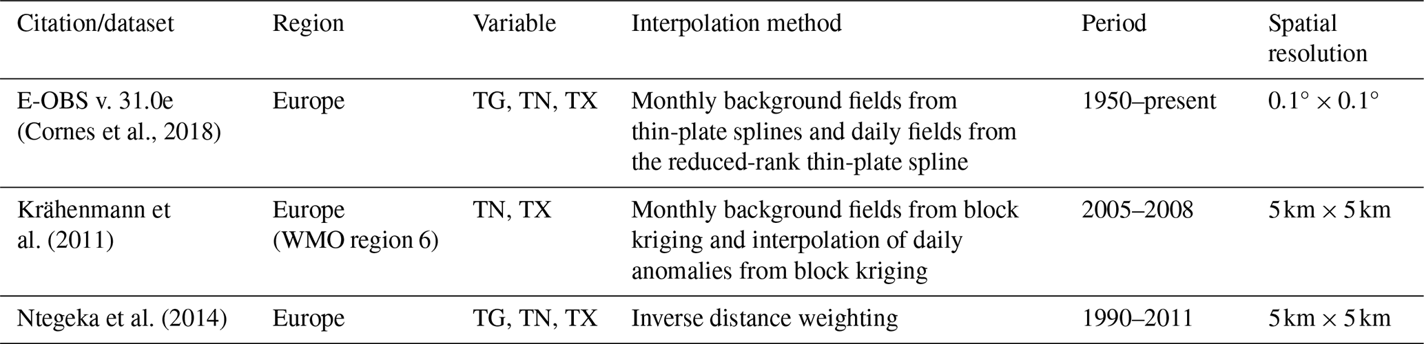
Variables – TN: daily minimum temperature, TG: mean daily temperature, TX: maximum daily temperature.

As shown in Table 2, there is an extensive range of methods used in the calculations, starting from the nearest-neighbour (NN) approach through linear interpolation aided with inverse distance weighting (IDW), distance weighting interpolation, thin-plate splines, kriging, external drift kriging, inverse distance weighting, optimal interpolation, or combined methods. In most cases, the resolution rarely reaches 1 km² and is usually restricted to 5 km² or larger. In central Europe, there are few daily databases of meteorological variables with a resolution higher than 5 km² and spanning at least 30 years, and only Swiss datasets are routinely updated (MeteoSwiss, 2025). This shows a need to produce gridded datasets of essential thermal characteristics on a daily scale covering the most extended possible period and utilising all possible verified quality station data. Thus, for the reasons stemming from the needs of potential end users and the scientific community, it is crucial to make an effort to provide such data for Poland.

Table 2 This table lists national gridded datasets containing temperature variables with at least daily temporal resolution.

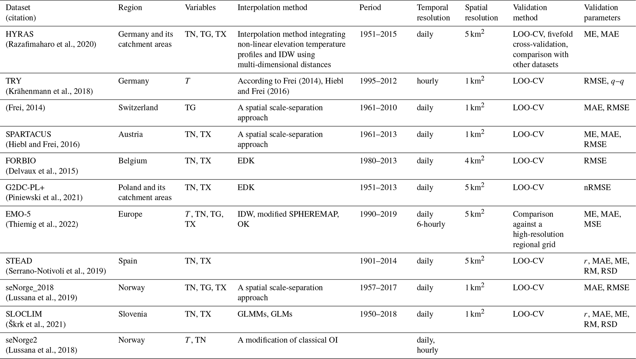
Variables – TN: daily minimum temperature, TG: mean daily temperature, TX: maximum daily temperature, T: sub-daily temperature. Interpolation methods – OK: ordinary kriging, OI: optimal interpolation, EDK: external drift kriging, IDW: inverse distance weighting, GLMM: generalised linear mixed models, GLM: generalised linear models. Validation methods – LOO-CV: the leave-one-out cross-validation. Validation metrics – r: correlation, (n)RMSE: (SD-normalised) the root-mean-square error, RMSD: the root-mean-square difference, MAE: the mean absolute error, ME: the mean error (bias), RM: the ratio of means, RSD: the ratio of standard deviations, SD: standard deviation.

The spatial resolution of most NMHS station networks is limited, and in the case of Poland, it is ca. 50 km² (depending on the relief). This is a severe impediment in the adaptation or mitigation analyses, preventing the proper assessment of climate variability. The increasing availability and application of high-resolution regional climate models (RCMs), including convection-permitting models (CPMs), necessitate corresponding high-resolution observational datasets for robust evaluation and allow for more direct comparisons and validation. The research aims to develop a gridded database of daily mean, maximum, and minimum temperatures (hereafter denoted as TG, TX, and TN, respectively) with a spatial resolution of 1 km² (Jaczewski et al., 2024). The gridding procedures involved the application of RBFs (radial basis functions) with several covariates, and the procedure's results were the subject of thorough comparison with in situ measurements to ensure the ability to reproduce the original climate characteristics variability. The research outcome in netCDF format database covers the 1951–2020 period, thus comprising 70 years of systematic measurements in the Polish NMHS network. The study's main purpose is to provide a high-temporal-and-spatial-resolution climate dataset for Poland, initially consisting of temperature variables. The provided methodology is the basis for introducing subsequent variables available from the network to the following versions of the dataset and will be improved by relying on the gained experience.

2 Data and methods

2.1 Station data

Using a long series of meteorological data makes it possible to carry out analyses related to the impact of the variability of meteorological conditions over a selected area on various sectors of human activity. Ensuring data quality is crucial in this case. IMGW-PIB has taken steps to develop complete information on the daily variability of thermal and precipitation conditions in Poland since 1951. The analysis and prepared data series include information on the daily values of the following meteorological variables: average daily air temperature, maximum daily air temperature, and minimum daily air temperature. The routine measurements from SYNOP and CLIMAT stations are subject to formal checks based on WMO standards (World Meteorological Organization, 1993). On the other hand, WMO have justified different methods of calculating the characteristics, particularly the average daily air temperature. The methods varied in different periods and depended on the stations' measurement programme, which was different at synoptic and climatological stations and is the main source of the series' inhomogeneity. One method of calculating the average temperature was necessary to compare data and ensure consistency across the available range of stations in the whole period. The same method was used to calculate the daily mean temperature following the one used for the Polish climatological stations since 1996:

$$\begin{array}{}\text{(1)}& \text{TG}={\displaystyle \frac{\text{T06}+\text{T18}+\text{TX}+\text{TN}}{\mathrm{4}}},\end{array}$$

where T06 and T18 are measurements at 06:00 and 18:00 UTC, respectively; TX is the daily maximum temperature, and TN is the daily minimum temperature. The day for TX and TN readings begins at 18:00 UTC of the previous day. This way, consistent information was obtained on the spatial variability of thermal conditions throughout the country in the multiannual period. In this way, the so-called uniform air temperature data were elaborated for 347 stations (Fig. 1). Additionally, this approach mitigated inconsistencies introduced by network automatisation since the 1990s. Mostly, interpolated gridded datasets developed for climate applications rely on homogenised station series. The homogenisation of daily series is more complicated than on a monthly scale. The procedure must consider weather variability to incorporate stations' metadata and support higher-order adjustments. Existing homogenisation techniques regard these issues, but their application to daily data is still developing (Killick et al., 2022).

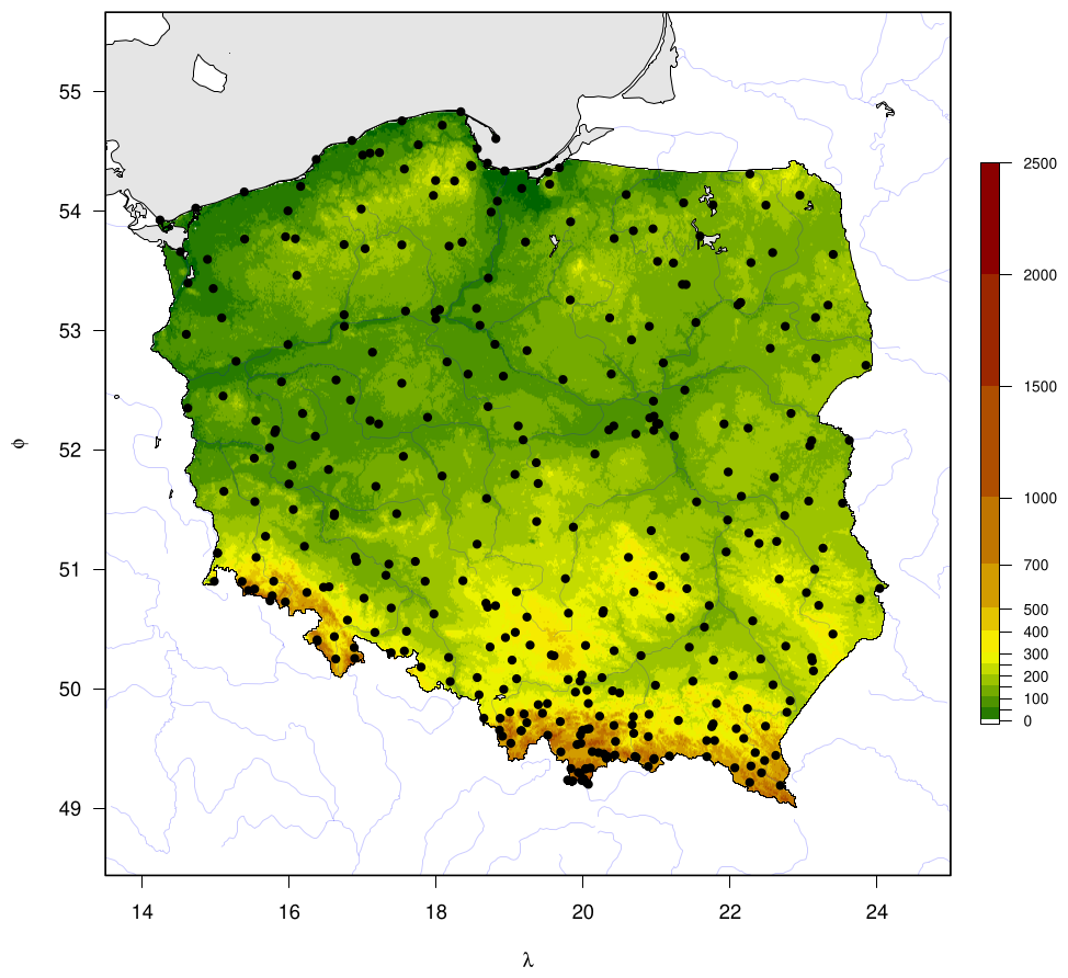
Figure 1 Orography and spatial distribution of meteorological stations in Poland with temperature time series in the 1951–2020 period.

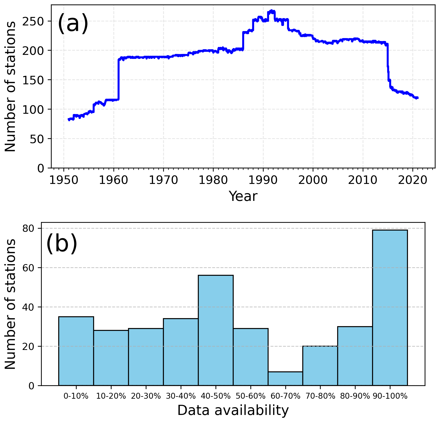
It should be noted that daily data availability varies from 1951 to 2020. A daily number of stations available for spatial interpolation is presented in Fig. 2a. The number of stations increased up to the late 1980s and early 1990s, resulting in a maximum number of uniform data at 268 records. Since the late 1990s, spatial coverage has degraded to only 119 locations. The number of stations by data availability is presented in Fig. 2b. Nearly 80 stations allowed for more than 90 % of records, and half of the locations overlapped for more than half of the period. Neither possible degradation in temporal consistency nor missing value filling was considered in this study.

Figure 2 Number of daily records (a) and stations by data availability ranges (b).

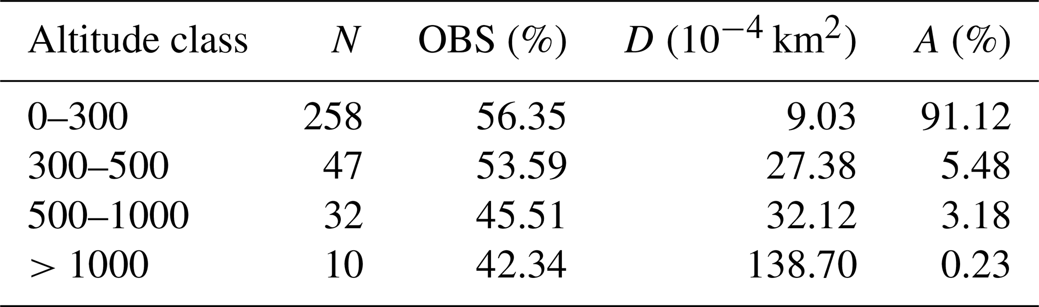
The station density in Poland is relatively low compared to other European countries, reaching nearly one station per 1000 km² in the year when the number of operating stations was the highest. Most stations are located in the lowland area, which occupies most of the country. Meteorological networks in mountainous regions across many countries are often sparse, but this is not the case in Poland. The station density in the Polish mountains, covering 0.23 % of the country (area with altitude exceeding 1000 m a.s.l.), is relatively high compared to the lowland and is occupied by 10 stations (Table 3), resulting in station density higher by an order of magnitude in these regions. On the other hand, data availability decreases with altitude from more than 56 % in the lowlands to 42 % in the highest mountains on average.

Table 3 The data records statistics by altitude ranges (m a.s.l.). N: number of stations, D: station density, OBS: percentage of available records, A: percentage of country area occupied by grid points.

2.2 Spatial interpolation

To interpolate the temperature data from the relatively sparse meteorological stations across our area, we employed radial basis functions (RBF). Referenced in Tables 1 and 2, the temperature datasets of high spatial and temporal resolution often use alternative interpolation methods, and RBFs have been successfully applied for interpolation station observational data in meteorology (Antal et al., 2021; Fathizad et al., 2017; Piri, 2017; Ryu et al., 2024; Saaban et al., 2013; Wang et al., 2014; Yang and Xing, 2021) or hydrology (Gao et al., 2022; Wypych and Ustrnul, 2011). The RBF interpolation models have also been used in agricultural applications for prediction purposes (Rocha and Dias, 2018, 2019). RBF interpolation method could be defined by Eq. (2):

$$\begin{array}{}\text{(2)}& F\left(r\right)={\sum }_{j=\mathrm{1}}^m{\mathit{\alpha }}_j\mathit{\phi }\left(r_j\right),\end{array}$$

where α_j is the weights, φ(r_j) RBF function of the distance r_j between interpolation point to m sample points and r is the Euclidean vector (coordinates) of the interpolation point. Selecting the appropriate RBF function determines the accuracy of the interpolation. Different RBF functions were found to be suitable for the interpolation of temperature data (Piri, 2017; Ryu et al., 2024; Saaban et al., 2013). In our study, six RBFs were used and are given as follows:

$$\begin{array}{}\text{(3)}& {\displaystyle }\text{Linear. }\mathit{\phi }\left(r_j\right)=r_j\text{(4)}& {\displaystyle }\text{Cubic. }\mathit{\phi }\left(r_j\right)=r_j^{\mathrm{3}}\text{(5)}& {\displaystyle }\text{Thin-plate spline. }\mathit{\phi }\left(r_j\right)=r_j^{\mathrm{2}}\log r_j\text{(6)}& {\displaystyle }\text{Gaussian. }\mathit{\phi }\left(r_j\right)=e^{-{\left(\frac{r_j}{\mathit{\beta }}\right)}^{\mathrm{2}}}\text{(7)}& {\displaystyle }\text{Multiquadric. }\mathit{\phi }\left(r_j\right)=\sqrt{\mathrm{1}+{\left({\displaystyle \frac{r_j}{\mathit{\beta }}}\right)}^{\mathrm{2}}}\text{(8)}& {\displaystyle }\text{Inverse multiquadric. }\mathit{\phi }\left(r_j\right)={\displaystyle \frac{\mathrm{1}}{\sqrt{\mathrm{1}+{\left(\frac{r_j}{\mathit{\beta }}\right)}^{\mathrm{2}}}}}\end{array}$$

Here, β is the shape parameter. In the three-dimensional space, the Euclidean distance is given by

$$\begin{array}{}\text{(9)}& r_j=\sqrt{(x-x_j{)}^{\mathrm{2}}+(y-y_j{)}^{\mathrm{2}}+(z-z_j{)}^{\mathrm{2}}},\end{array}$$

where $(x,y,z)$ represent the coordinates of interpolation point. For a given dataset of m points, the interpolated n values are obtained by following the linear system of n equations:

$$\begin{array}{}\text{(10)}& F(x_i,y_i,z_i)={\sum }_{j=\mathrm{1}}^m{\mathit{\alpha }}_j\mathit{\phi }\left(r_j\right),i\in \mathit{\left\{}\mathrm{1}\mathrm{\dots }n\mathit{\right\}}.\end{array}$$

In our case, m corresponds to the number of stations varying temporally according to daily data availability, x and y correspond to geographical coordinates, and z is elevation. Generally, the coordinates and elevation are treated as predictors, and more explanatory variables can be introduced to the interpolation procedure. It is identified that the incorporation of elevation data as an auxiliary variable accounts for orographic effects, mitigates the smoothing effect, and improves the representation of gradients in daily gridded datasets (Brinckmann et al., 2016; Delvaux et al., 2015; Frei, 2014). Choosing the optimal value of the shape parameter is not a straightforward task (Fasshauer and Zhang, 2007). Often, this problem is paved over in the application studies, and it should be assumed that the value has been chosen as the mean distance between the nearest points (observational stations) as it is implemented in numerical tools as the default option. We have used this value in the interpolation procedure with Gaussian, multiquadric, and inverse multiquadric functions. The shape parameter ranges from 15 to 22 km for the daily maximum (268 stations) and minimum (81 stations) number of data records, respectively.

2.3 Temporal and spatial reference of the dataset

The dataset consists of daily gridded TN, TG, and TX covering Polish territory at 1 km² spatial resolution for 1951–2020. The interpolation is in the grid projected in the PUWG 1992 (EPSG:2180) coordinate reference system. The elevation data originate from the digital terrain model (DTM) for Poland (DTM 100 m, 2023), corresponding to the digital elevation model (DEM). Given the data, simplify the interpolation procedure as all three coordinates (x, y, and z) are in the same units (meters). Additionally, we avoided topography interpolation by defining the grid as every 10th x and y coordinate of the 100 m×100 m DTM mesh and assigning the average elevation values over the 1 km² surrounding area.

3 Results

3.1 Validation

The most popular technique for validating interpolation techniques is leave-one-out cross-validation (LOO-CV). It involves using all except one point of observation data for interpolation, and the remaining station is used for validation. The main drawback of this method is relatively high computational time as the procedure has to be repeated for every station, which has to be removed from the whole dataset. Another cross-validation method, the hold-out technique (HO-CV), is used to avoid long calculations. This method splits the observation data into interpolation and validation sets. Daily, 95 % of stations are randomly removed, and 5 % are used for validation. The procedure is repeated every day. The hold-out technique was chosen to select the RBF function, and the LOO-CV technique was used to evaluate results with the selected RBF function.

To evaluate the accuracy of the interpolated data, mean error (ME), root-mean-square difference (RMSD), centred RMSD (cRMSD), and Pearson's correlation coefficient have been used. The latter two metrics and standard deviations have been presented through Taylor's diagrams. The tables with numeric results rounded to two decimal points were provided, including differences between the 5th and 95th percentiles. The observed data were compared to the nearest interpolation grid point, and validation was performed monthly. The following equations define the metrics:

$$\begin{array}{ll}\text{(11)}& {\displaystyle }& {\displaystyle }\text{Mean error (bias). }\text{ME}={\displaystyle \frac{\mathrm{1}}{N}}{\sum }_{n=\mathrm{1}}^N(I_n-O_n){\displaystyle }& {\displaystyle }\text{Root-mean-square difference. }\\ \text{(12)}& {\displaystyle }& {\displaystyle }\text{RMSD}=\sqrt{{\displaystyle \frac{\mathrm{1}}{N}}{\sum }_{n=\mathrm{1}}^N(I_n-O_n{)}^{\mathrm{2}}}{\displaystyle }& {\displaystyle }\text{Centred root-mean-square difference. }\\ \text{(13)}& {\displaystyle }& {\displaystyle }\text{cRMSD}=\sqrt{{\displaystyle \frac{\mathrm{1}}{N}}{\sum }_{n=\mathrm{1}}^N\left[\right(I_n-\stackrel{\mathrm{‾}}{I})-(O_n-\stackrel{\mathrm{‾}}{O}){]}^{\mathrm{2}}}{\displaystyle }& {\displaystyle }\text{Pearson's correlation coefficient. }\\ \text{(14)}& {\displaystyle }& {\displaystyle }r={\displaystyle \frac{\frac{\mathrm{1}}{N}{\sum }_{n=\mathrm{1}}^N(I_n-\stackrel{\mathrm{‾}}{I})(O_n-\stackrel{\mathrm{‾}}{O})}{{\mathit{\sigma }}_I{\mathit{\sigma }}_O}}\end{array}$$

Here, I and O denote interpolated and observed values, N is the number of observations, and σ_I and σ_O are standard deviations of interpolated and observed values, respectively. $\stackrel{\mathrm{‾}}{I}$ and $\stackrel{\mathrm{‾}}{O}$ are the means of interpolated and observed values, respectively.

3.2 Hold-out cross-validation (HO-CV)

The validation process results are presented using Taylor diagrams, which provide a quick statistical summary of how well the interpolated and observed data align. We show mean values of correlations, centred root-mean-square differences, and standard deviations for all RBF methods every month. While a common approach is to normalise the differences and standard deviations of interpolated data by the standard deviations of observations, it may negatively impact the clarity of the figures in our case. As the variability (SDs) of the variables differ across seasons and variables, we can present the results for all methods and temperatures in the exact figure.

The linear approach is undoubtedly the most accurate for all months and variables (Fig. 3). Only for TX in April and August do the values interpolated by the inverse multiquadric RBF function agree similarly with observations. The mean cRMSD for the linear RBF function is lower than 1 for TG and TX, but for TN, it exceeds 1. This method also sustains observed variability as the standard deviations of interpolated and observed values are similar. Correlations exceed 0.95 for all variables and months except TN from April to September. These results allowed us to proceed further only with the linear method.

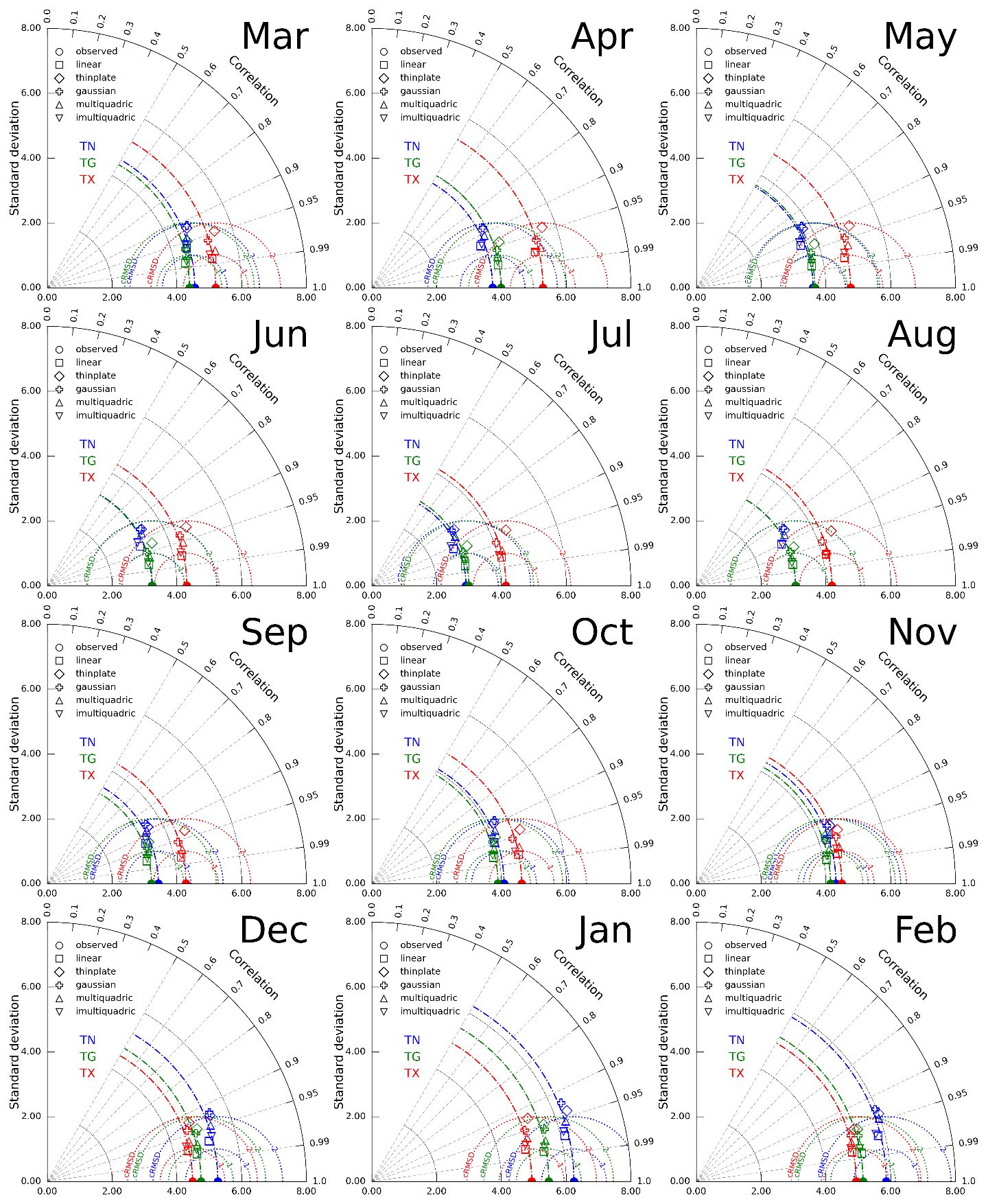
Figure 3 Taylor diagrams for HO-CV of spatial interpolation of TN, TG, and TX by different RBF functions. The colours correspond to the variables in the following order: blue, green, and red. Filled circles on the x axis and dot-dashed minor arcs represent standard deviations of observed values; dotted semicircles correspond to cRMSD values. The azimuthal position represents the correlation coefficient. The marker's shape describes the type of RBF used for interpolation. For a detailed explanation of the diagram's principles, see Fig. 2 in Taylor (2001).

3.3 Leave-one-out cross-validation (LOO-CV)

LOO-CV has emerged as a widely used verification methodology for spatial interpolation techniques in meteorology and climatology. In executing this method, the given station is removed from the daily observation dataset, and the remaining stations are used to construct the interpolated field. The value at the grid nearest to the removed station is compared to the observed value. The procedure is repeated for all stations and days in the analysed period, and the mean values of the comparison metrics are presented in Taylor diagrams (Fig. 4). The charts depict the level of agreement between the observed and interpolated values. The results show that the best agreement is achieved for TG in winter and spring, with the lowest cRMSD and the highest correlation values. Although the agreement for TX is slightly worse than the mean, it is still relatively favourable overall, with the best agreement seen in autumn. However, the interpolation methodology performs worse in capturing the nuances of TN, with the best agreement observed in winter. It is important to note that the variability in all temperatures is preserved in the standard deviation, with similar values between observed and interpolated data.

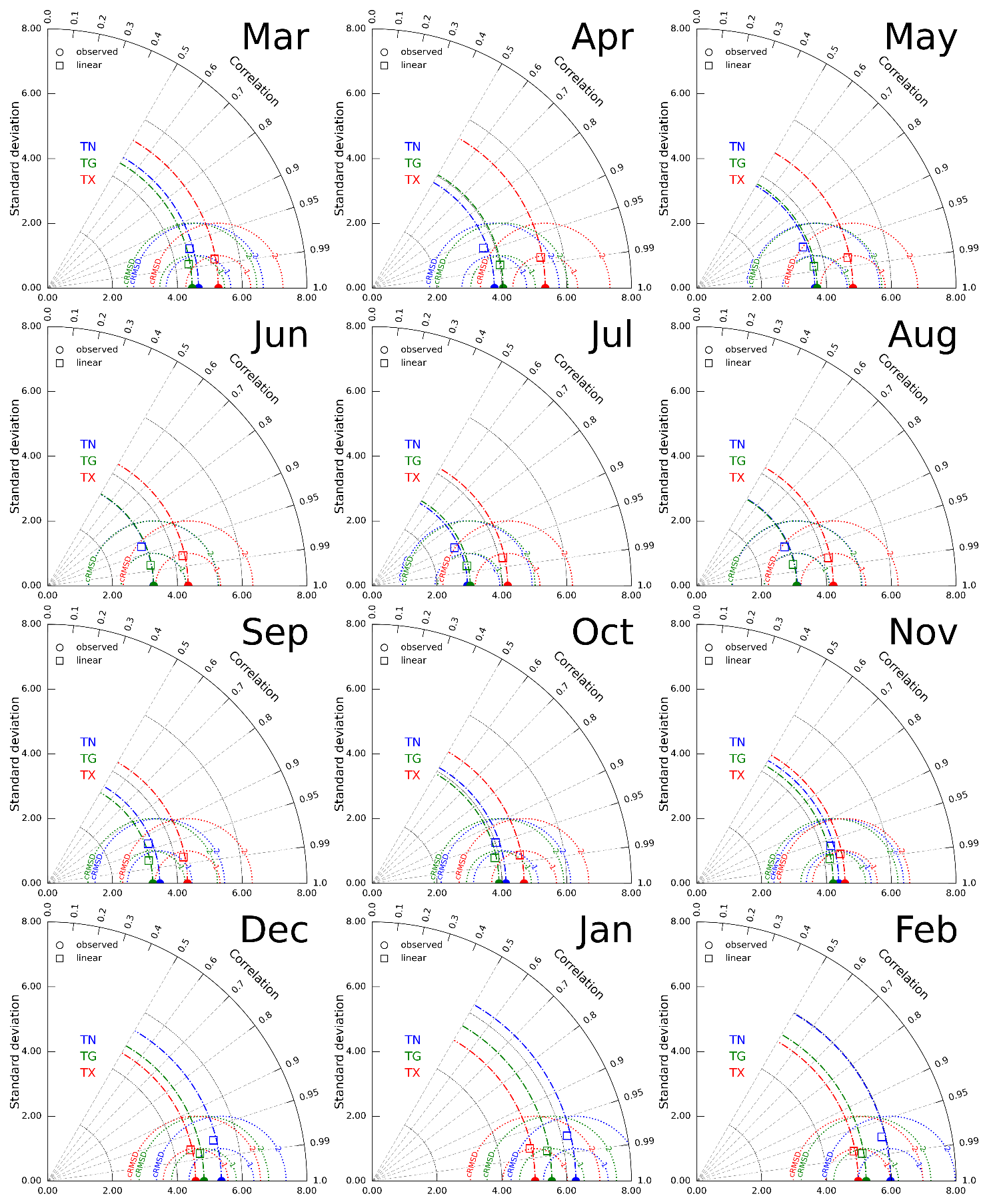
Figure 4 Taylor diagrams for LOO-CV of spatial interpolation of TN, TG, and TX by linear RBF function. See Fig. 3 for more details.

Table 4 provides the set of quality metrics for RBF interpolation. Mean error (ME, a.k.a. bias) is minimal and, for all variables, does not exceed 0.03 with minuscule interannual variability. TN is characterised by the highest RMSD, reaching, on average, 1.29. The RMSD annual value for TG equals 0.75, whereas for TX, it is slightly higher (0.92). The highest average annual value is recorded for TN (1.29). For all analysed variables, Pearson's correlation coefficient is very high. An annual course ranges from 0.94 (TN) to 0.98 (TG, TX). Only in the case of TN is there a slight seasonal variability, with the lowest values (0.91) in July and the highest (0.97) in winter (December–January). RM (the ratio of means) is close to 1 with a range of 0.99–1.01 for all months. RSD (the ratio of standard deviation) is very high, nearing 1 for all variables, pointing to slight variability underestimation. Slight seasonal variability is observed for TN, and lower values are seen in the summer. The difference in the values of the 5th and 95th percentiles suggests a slight underestimation in the case of Q95 and an overestimation for Q05. This pattern repeats for all variables (TN, TG, and TX), with the highest differences in average annual values recorded for TN.

Table 4 Overall monthly validation measures (OBS vs. gridded).

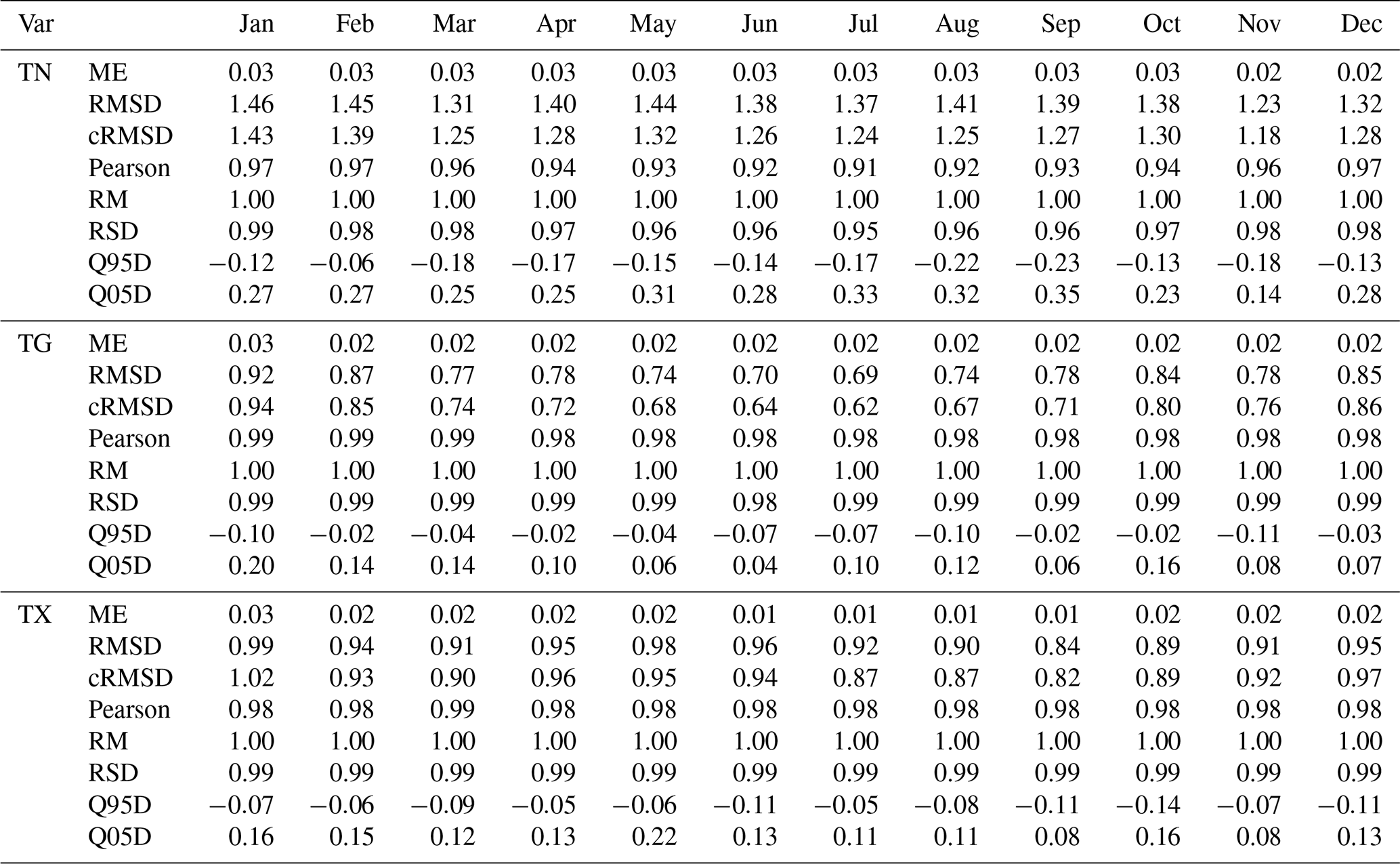
ME: mean error (K), RMSD: the root-mean-square difference (K), cRMSD: centred root-mean-square difference (K), Pearson: Pearson's correlation coefficient, RM: the ratio of means, RSD: the ratio of standard deviations, Q95D and Q05D: the difference in 95th and 5th between gridded and observed values (K).

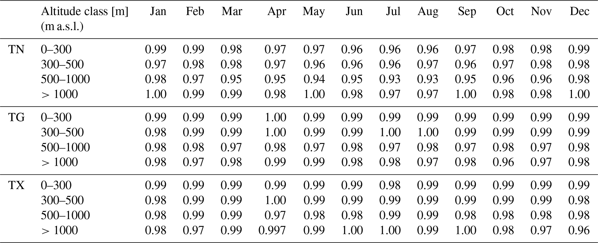
Verification of RBF interpolation quality based on RM for distinct altitude (m a.s.l.) classes confirms overall quality characteristics. A table is intentionally not shown as the values for particular stations are in the range of 0.992–1.008, resulting in 1.00 after rounding to two decimal places for all months and altitude ranges.

The ratio of standard deviation (RSD) showed slight variance underestimation (Table 5), the highest being for TN at 500–1000 m in summer. The ratio for TN also experiences the highest seasonal variability, where the smallest values are seen in summer and the highest in winter. Surprisingly, the cases of agreement close to perfect are seen most often at >1000 m.

Table 5 Overall monthly RSD values for station altitude classes.

4 Example applications of the datasets

4.1 Trend analysis

One of the most important features required from grid data, which is to be used in climatological analysis and subsequently in the application of climate adaptation schemes, is the ability to represent the trends of analysed variables. Figure 5 presents the interannual course of trend coefficients for TG, TX, and TN at the nodes nearest to selected stations. The locations represent the low-lying stations (Hel, Łódź-Lublinek, Wrocław) and stations from mountainous areas: Zakopane (∼900 m a.s.l.) and Kasprowy Wierch (1984 m a.s.l.). There is a striking complete coherence of trend coefficients for stations outside the mountainous areas, where the values are virtually equal when comparing observational (OBS) and interpolated (RBF) data. More significant discrepancies occur in the mountainous regions, but the differences are within the range of 0.05 °C per 10 years. In the case of Zakopane, there is a systematic difference in the case of minimum temperature (TN) with slightly higher trend coefficient values for observational data. This situation, but to a much lower extent, is also visible in mean temperature (TG). In the case of Kasprowy Wierch (a station which is a mountain observatory and located in the terrain of highly variable relief), the differences in trend coefficients present themselves in the case of all analysed variables. For TX, there is a bias with higher trend values for interpolated values, most visible in cold months (with the difference not exceeding 0.05 °C per 10 years, however). It is less evident for TG, where greater bias is recorded for winter/cold months (October–March), with much more minor differences for the warm half of the year. Minimum temperature exhibits a reversing pattern with higher values of observed trends in the warmer part of the year and reversed bias (RBF>OBS) during cold months (October–March). It should be noted that the significance of trends based on interpolated data follows the results for observed trends. Exceptionally, non-significant observable TX trends in January and February appear significant for interpolated data in Kasprowy Wierch. Conversely, significant observable TN trends in November and December are non-significant in Zakopane based on interpolated data. The above examples confirm the possibility of using the RBF gridded data to analyse multiannual air temperature variability in Poland, including even the areas of high relief variability.

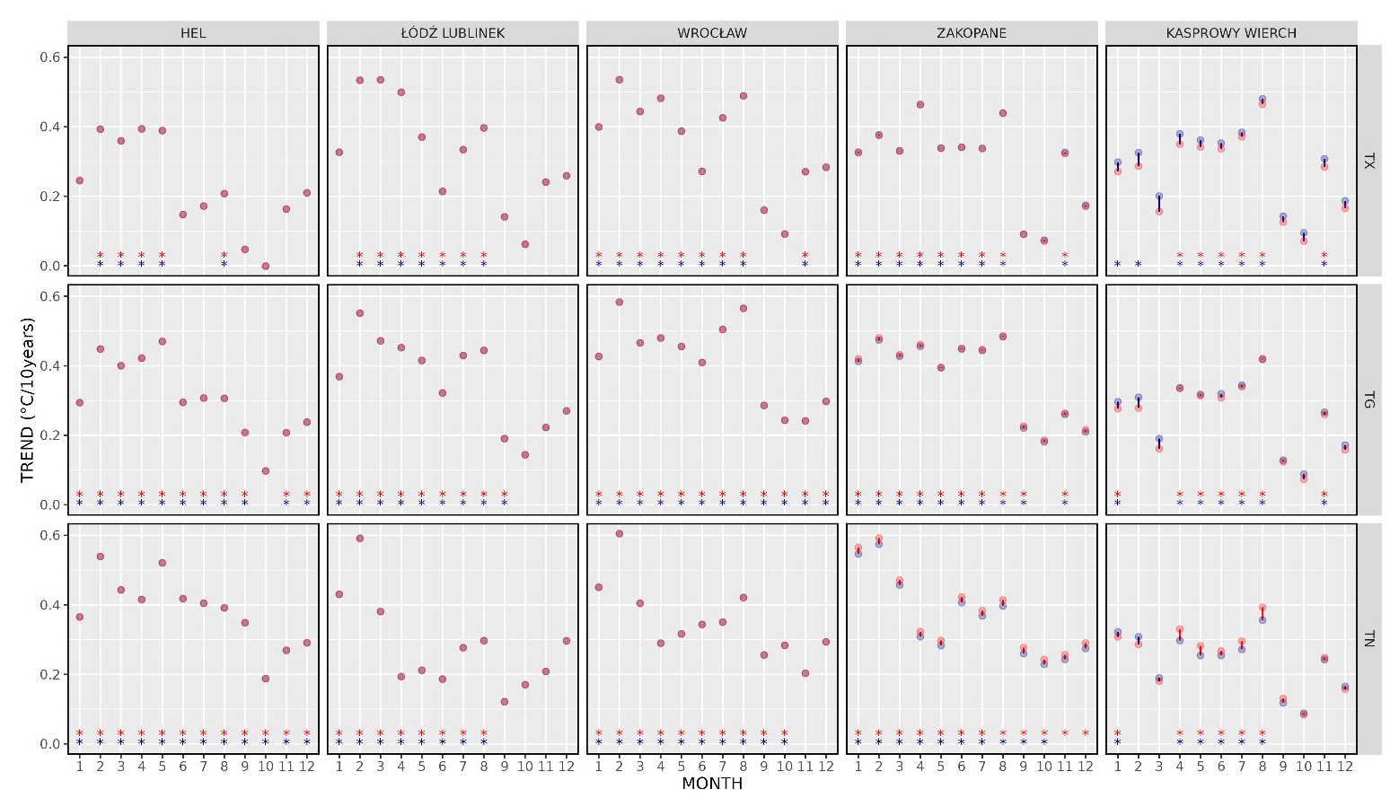
Figure 5 Monthly trend coefficients (°C per 10 years) at selected stations for 1951–2020. Red dots: OBS, blue dots: RBF. The asterisks in the corresponding colours indicate significant trends.

4.2 Extreme analysis

The daily temporal resolution of the dataset allows the possibility of deriving multiple statistical characteristics with very high spatial resolution and detailed analysis of the thermal characteristics on the regional or even local scale (counties, small cities, or villages). For example, Fig. 6 provides an insight into the spatial variability of the TX 90th quantile in Poland for two 30-year periods: 1951–1980 and 1991–2020 in January and July. As expected in January, there is a substantial shift in the values of TX. The overall range of recorded values changes from −1.4 to 7.7 °C (1951–1980) and from 1.1 to 10.6 °C (1991–2020), which indicates a 2.5 °C shift in the lower boundary and 2.9 °C in the upper limit of the spatial distribution, indicating higher variability in the maximum values of TX. The overall spatial pattern of the TX 90th quantile remains relatively intact. However, the shift is visible in the whole country. In July, the change in the range of the TX 90th quantile also reaches 2 °C and is from 13.6 to 30.8 °C in the case of the first sub-period and from 15.6 to 32.9 °C for the second one. This is also clearly visible for nearly the whole country but less pronounced in the mountains and the vicinity of the Baltic Sea.

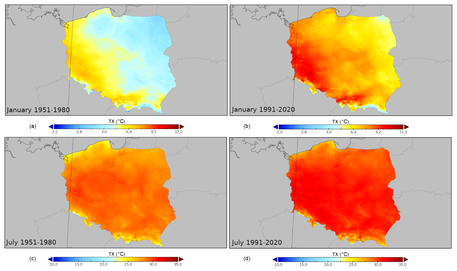
Figure 6 Spatial variability of the 90th quantile of TX in Poland for selected 30-year periods (1951–1980, a, c; 1991–2020, b, d) in January (a, b) and July (c, d).

Figure 7 presents a similar analysis, but in this case, it is for the minimum temperature (TN) probabilistic characteristics. Again, the comparison between selected 30-year periods shows a substantial change in the derived values concordant with the observed trends in the TN values in central Europe (Ustrnul et al., 2021). For January, the change in the range of recorded values is 1.3 °C (an increase from −21.1 to −19.8 °C) in the case of the lower limit and 1.2 °C (an increase from −8.1 to −6.9 °C) for the upper limit. Also, in this case, the overall observed change is characteristic for nearly the entire country, except the Baltic Sea coast, where the positive change is less pronounced. In July, the overall change in the range of values is +2.2 °C (for minimum) and +0.9 °C (for maximum values).

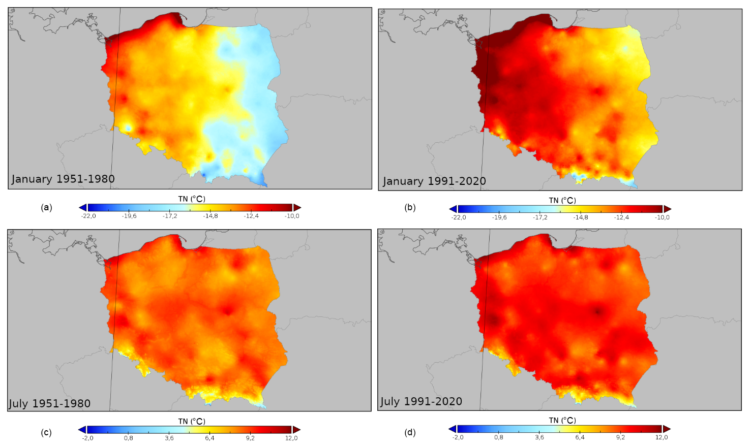
Figure 7 Spatial variability of the 10th quantile of TN in Poland for selected 30-year periods (1951–1980, a, c; 1991–2020 b, d) in January (a, b) and July (c, d).

Figure 8 and Table 6 provide an additional example of the potential application of the dataset. In this case, we present it for the whole country. Still, with the spatial resolution of 1 km², it is equally applicable for the counties or even smaller areas desired by, for example, organisations preparing climate adaptation plans. The analysis presents the differences between the values of selected characteristics (in this case, extremes: the 90th quantile of TX and 10th quantile of TN) for selected 30-year periods: 2020–1991 and 1980–1951. The map indicates the areas where the observed climate change (expressed as the difference in temperature's extreme characteristics) was the most pronounced and also allows for a further insight into the spatial variability in chosen metrics.

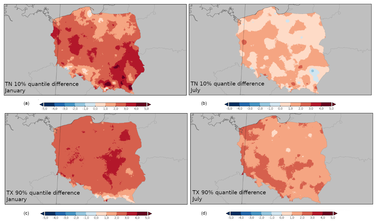
Figure 8 January (a, c) and July (b, d) differences (°C) between the values of the TN 10th quantile (a, b) and the TX 90th quantile (c, d) for the periods of 1991–2020 and 1980–1951.

Table 6 Essential field characteristics (mean, quantiles: 0.1, 0.5 and 0.9) of TX 90th and TN quantile differences (°C) averaged over the country area between 1951–1980 and 1991–2020.

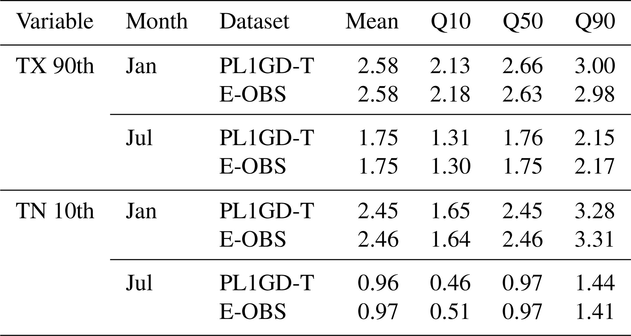
A further analysis of such fields provides additional context. Table 6 shows the precise information on the area average change in the values of the abovementioned characteristics, extended by comparison to the E-OBS dataset. The analysis not only refers to the averages but, thanks to the calculation of the percentiles provides information on the distribution of the shift magnitude in a given area. In this case, providing the percentiles' values cutting off the extreme 10 % of grid point values. In the case of the PL1GD-T dataset, it shows that the area average change for TX and TN quantiles (10th and 90th, respectively) was relatively similar in January (ca. +2.5 °C) and much lower in July; however, in July, this change was more pronounced for TX (+1.75 °C) than TN (+0.96 °C) extremes. In the case of the TX 90th quantile, 10 % of the analysed area experienced a shift of over +3.00 °C in January. For June, this value is lower and equals +2.15 °C. For the TN 10th quantile, 10 % of the area had a shift more significant than +3.28 °C in January, whereas in July, it was much lower (+1.44 °C). The lower quantile (10th) of the TX 90th and TN 10th quantiles, showing the threshold for the area experiencing less or equal values, also indicates a more pronounced shift magnitude in January than in July. It is worth noting that in the case of TX, in the 90th quantile in January, only 10 % of the country experienced a change lower than +2.13 °C (1.31 °C in July). In the case of TN 10th quantile, this is only +0.46 °C in July and +1.65 °C in January.

5 Data availability

PL1GD-T – gridded dataset of the mean, minimum, and maximum daily air temperature at the level of 2 m for the area of Poland at a resolution of 1 km×1 km – is publicly available in the public repository of the Institute of Meteorology and Water Management – National Research Institute under the https://doi.org/10.26491/imgw_repo/PL1GD-T (Jaczewski et al., 2024). The data are archived as netCDF files in 10-year chunks for every variable separately. The resulting datasets consist of fields with values rounded to one decimal, with data values encoded as integers with a scale factor of 0.1. It allowed the files' size to be decreased by a factor of 2. The naming convention is variable_startyear_endyear.nc with variable prefixes “tn”, “tg”, and “tx” for minimum, mean, and maximum temperature, respectively. The netCDF files comply with the CF-1.6 convention.

6 Summary and outlook

The paper presents a comprehensive study on developing a high-resolution gridded dataset of daily air temperatures at 2 m above the ground (minimum, mean, and maximum) over Poland from 1951 to 2020 with a spatial resolution of 1 km². The dataset was created using quality-controlled observations from ground weather stations. Hold-out cross-validation was chosen to select appropriate radial basis functions (RBFs) for interpolation. Leave-one-out cross-validation assessed product quality on a seasonal, monthly, and station basis. The findings indicate the best performance for mean temperature in winter and spring, with high correlation and low root-mean-square deviation. Although the performance for maximum temperature is slightly below average, it still shows relatively good agreement, especially in autumn. The method is less successful at accurately capturing minimum temperature, with the best results seen in winter. The analysis also confirms that the standard deviation of temperatures, representing variability, is consistent between observed and interpolated data. All variables have a bias that does not exceed 0.03, with minimal interannual variability. Pearson's correlation coefficient is very high, ranging from 0.94 to 0.98. The difference between the 5th and 95th percentiles suggests a slight underestimation for Q95 and overestimation for Q05. There is a noticeable increase in seasonal RMSD variability with altitude, with relatively small interannual differences at a lower altitude and the greatest in the case of the highest altitude class. Mean values are preserved, and the interpolated data's standard deviation is slightly lower. Finally, we show an example of the application of the resulting gridded product in the field of climate change.

The validation results demonstrate the dataset's accuracy and suitability for climatological applications. However, some limitations and potential areas for improvement have been identified. Notably, while computationally efficient, the RBF interpolation method may smooth out extremes and underestimate spatial variability, particularly in areas with complex terrain. Future work could explore refining the RBF implementation to mitigate this, such as by investigating adaptive shape parameters that vary spatially based on station density or terrain complexity, employing anisotropic RBFs to account for directional dependencies in temperature variability or using an ensemble of RBF interpolations with varying parameters to capture uncertainty in the interpolation. Furthermore, while beyond the scope of this study, future releases will include a measure of uncertainty for all estimates, enhancing the dataset's utility for users. In addition, future work may consist of homogenising the input station data. The availability of detailed station metadata (https://klimat.imgw.pl/pl/meta-dane/, last access: June 2025) will be crucial for applying appropriate homogenisation techniques. Finally, given the dataset's demonstrated value, we envision transitioning to a quasi-routine production system and incorporating other surface meteorological variables, enabling regular updates and wider accessibility for the climate research community and related applications.

This open-access dataset is crucial for climate change impact studies on a smaller scale and can serve a wide range of users, including researchers, administrative bodies, and society. One important application of such a dataset is serving as reference data for bias correction of regional dynamical downscaling results (e.g. EURO-CORDEX initiative) to elaborate effective adaptation and mitigation strategies.