The Italian contribution to the Synoptic Arctic Survey programme: the 2021 CASSANDRA cruise (LB21) through the Greenland Sea Gyre along the 75° N transect

In September 2021, as part of the Italian Arctic research programme, a multidisciplinary cruise along the 75th parallel north through the Greenland Sea Gyre was conducted aboard the Italian icebreaker Laura Bassi in the framework of the CASSANDRA project, which also contributed to the Synoptic Arctic Survey (SAS) 2020/22. The cruise took place during the period of the lowest summer sea ice extent ever measured. The data show strong horizontal gradients with temperatures between 1.5 and 9.0 °C and salinity between 30 and 35. Warm and salty Atlantic Water (AW, θ > 3.0 °C, S around 35) dominates on the eastern side of the transect in the upper 500 m with surface temperatures of 4.5–9.0 °C, while Polar Water (PW, θ < 0 °C, S < 33) occupies the surface layer (50–80 m) in the west. The intermediate layer (100–500 m) consists of mixed water, and below 500 m the deep water of the Greenland Sea and the Norwegian Sea predominates. The oxygen enrichment is higher in the intermediate layers, while the values in deep layers and western regions are lower (<300 µmol kg⁻¹). A stratified upper layer (30–50 m deep) with low surface nutrients, especially nitrate, is observed, while an accumulation of silicate occurs in deep water masses. The surface water in the eastern part of the transect has high pH_T and total alkalinity values due to photosynthesis and the presence of salty AW, while the fresh PW in the west has a lower alkalinity. Respiratory activity and organic matter concentrations (particulate/dissolved organic carbon) vary horizontally at the surface, decrease with depth, and increase slightly near the seafloor. A west–east gradient is also observed for δ¹⁸O and δD, with the ratios indicating the influence of freshwater at the surface near the Greenland coast. The abundance of prokaryotes decreases from the photic zone (<100 m depth) to the sea floor. Carbohydrates and carboxylic acids are identified as well-utilised polymers at every station and in every layer. Overall, the microbial enzyme patterns show a decrease from the surface to deeper layers, with some hotspots of metabolic activity at 20–40 m and in the aphotic layer. The enzyme patterns vary spatially, with activity peaks at the ends and in the middle of the transect. Phytoplankton biomass, expressed as chlorophyll a, varies across the transect, with higher values at the westernmost and easternmost stations. The micro-phytoplankton fraction dominates in PW, while the nano-phytoplankton fraction predominates in AW, even at the interface between the two water masses. Data of phytoplankton communities show low abundances and a dominance of nano-sized organisms, with diatoms being more abundant in the western part. Microzooplankton represents an important fraction of the planktonic community in this area, with tintinnids being the most important groups along the transect. Micrometazoans and aloricate ciliates are more abundant in the AW, resulting in higher biomass values at the eastern stations. Copepods are the most abundant mesozooplanktonic taxon both at the surface and in the upper 100 m water layer (97 % and 94 % of total mesozooplankton abundance, respectively), mainly represented by the genus Calanus.

The data are publicly available at the Italian Arctic Data Centre (IADC), see https://doi.org/10.71761/c082c3ca-40bf-42b1-a61a-7b3697ab2c5a (Bensi et al., 2024), https://doi.org/10.71761/f7474404-3331-43e5-883b-25755e94956d (Azzaro et al., 2024).

1 Introduction

The Greenland Sea, in the north Atlantic, is a region of deep ocean convection that contributes to the Atlantic Meridional Overturning Circulation (AMOC) and the exchange of water masses between the Atlantic and Arctic oceans. Its sensitivity to climate change remains uncertain, as the ecosystems of the subarctic Atlantic are particularly sensitive to global warming (Whitt, 2023). In fact, the Greenland Sea serves also as a hub for heat, salts, nutrients, carbon, and organisms between the Arctic, subarctic, and lower latitudes. Arctic and subarctic regions have experienced warming twice as fast as global warming over the past 50 years (Rantanen et al., 2022). This has led to significant environmental changes, including increasing wetness, reduced sea ice thickness and coverage, changes in snow cover, thawing of permafrost, and melting of the Greenland ice sheet (Carmack et al., 2015; Polyakov et al., 2017, 2023; Babb et al., 2023). These changes have created a positive feedback loop known as “Arctic amplification” which is likely to intensify in the future. Despite its crucial role in the global climate system, the Arctic Ocean remains poorly understood due to its remote location, harsh weather, and seasonal ice cover. The Arctic Ocean receives heat through the inflow of Atlantic Water (AW, with temperature (T) > 0 °C). AW flows northward transported by the Norwegian Atlantic Current (NAC) and the West Spitsbergen Current (WSC) along the eastern slope of the North Atlantic and crosses the Greenland Sea and Fram Strait, where it is partly deflected by the local circulation (Fig. 1). On the other hand, the Arctic outflow of Polar Water (PW, T < 0 °C), together with the sea ice export from the Arctic, is driven by the East Greenland Current (EGC, Chatterjee et al., 2018). Greenland freshwater flux shows a large seasonal variation, with peaks in July (4–6 times higher than in winter), but also a consistent increase since the 2000s (Dukhovskoy et al., 2019). Changes in annual and multi-year sea ice trends are also an important factor to consider when analysing the physical and biogeochemical conditions in the Greenland Sea. Sea ice extent and thickness in the Arctic regions have continuously decreased over the last four decades, and significant changes have also been observed in the Fram Strait since 2015 (de Steur et al., 2023). Since 2020, however, sea ice extent in the Fram Strait and marginal seas has shown a slight recovery in seasonal winter maxima (Onarheim et al., 2024). Open-ocean convection also occurs in the Greenland Sea during winter seasons. It is thought to represent a significant proportion of dense water production for the regions, even though a large variability in this process has been observed in recent decades, including changes in the depth of convection (Clarke et al., 1990; Simpkins, 2019; Brakstad et al., 2019). Overall, the predominant atmospheric conditions over the Arctic are characterised by the presence of high pressure (i.e. polar highs) over the western Arctic and low pressure over the Siberian region, which trigger the main anticyclonic wind regime. However, after 2007, a secondary dipole, characterised by higher sea level pressure over the Beaufort Gyre and the Canadian Archipelago along with lower sea level pressure over the Siberian Arctic, became dominantly positive, favouring reduced flows into the Arctic through the Fram Strait along with enhanced inflows through the Barents Sea Opening (Polyakov et al., 2023). Consequently, from 2007 to 2021, the predominant cyclonic atmospheric regime over the Arctic Ocean pushed large amounts of freshwater from the Siberian shelves into the Beaufort Gyre (Polyakov et al., 2023).

The cyclonic Greenland Sea Gyre (GSG) in the central Greenland Sea, which is mainly driven by large-scale cyclonic winds, contributes to the regulation of the inflow and outflow of AW and PW between the Atlantic and Arctic oceans (Chatterjee et al., 2018). The GSG, and the North Atlantic Subpolar Gyre (SPG), south of Iceland, have large implications for the large-scale changes in the subpolar and polar marine environment. A strong GSG triggers a northwestward shift of the subpolar front, which intensifies the poleward transport of Atlantic water towards the Fram Strait, Barents Sea, and Arctic Ocean (Chatterjee et al., 2018). In contrast, a weak phase (i.e. a negative index, see Fan et al., 2023) in the SPG enables the northward expansion of subtropical warm and saline waters, while a strong SPG feeds cold and fresh subpolar waters into the Atlantic inflow.

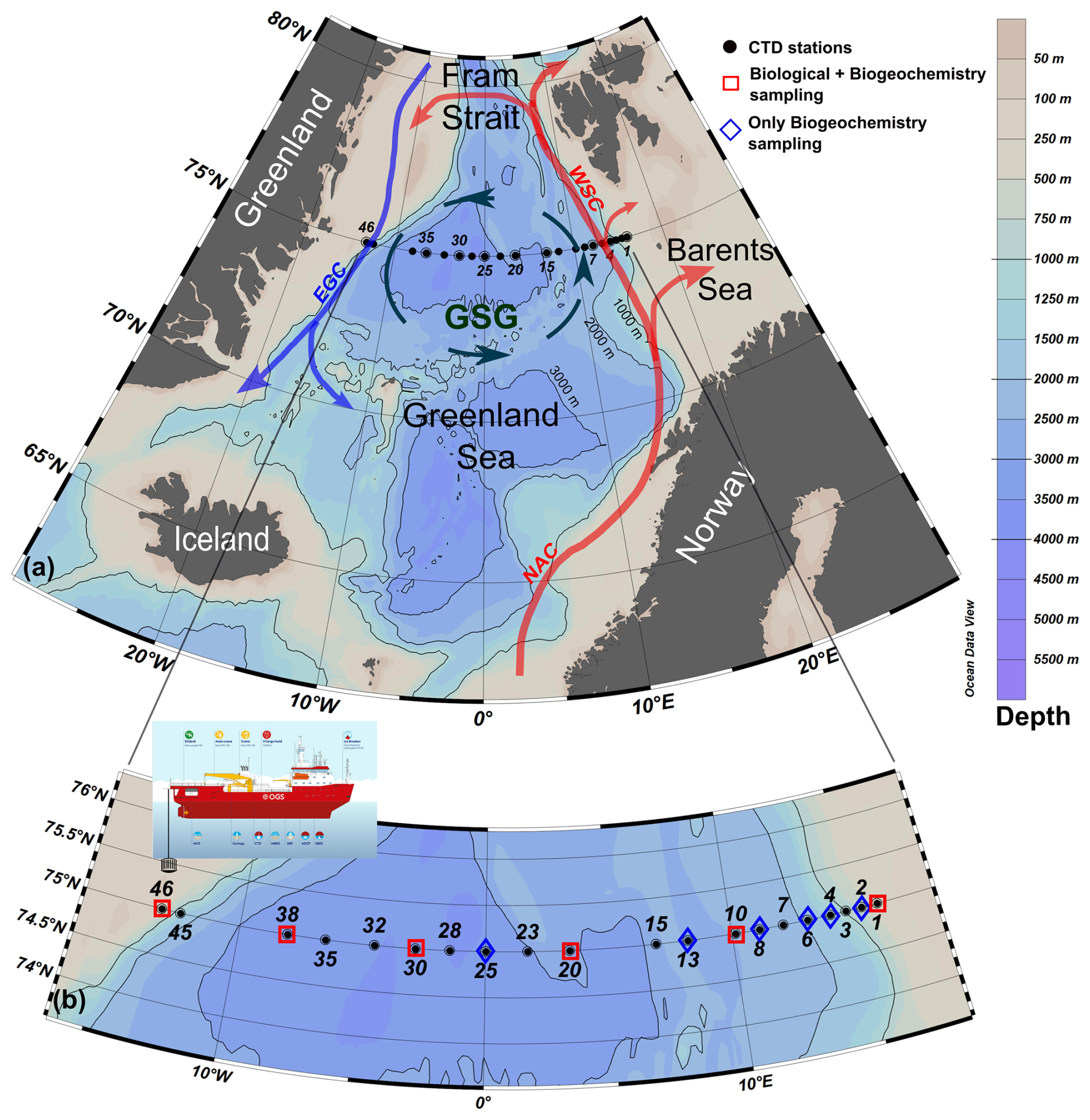
Figure 1 (a) Schematic of the general circulation in the Greenland Sea (GSG – Greenland Sea Gyre; WSC – West Spitsbergen Current; EGC – East Greenland Current; NAC – Norwegian Atlantic Current). (b) Distribution of hydrological (CTD) stations conducted during the LB21 CASSANDRA cruise (29 August–14 September 2021) with the positions of the physical (black dots) and biogeochemical and biological stations (blue and red symbols). Panels created with Ocean Data View (Schlitzer, 2024).

A time lag of 3–5 years is expected for the thermohaline anomalies to propagate in the Nordic seas (Fan et al., 2023) from the subpolar regions. In other words, while the GSG regulates the AW inflow into the Arctic, the SPG modulates the proportion of subtropical and subpolar waters moving at high latitudes. Wind forcing and heat loss combine to drive the full variability of the flow and water mass transformations in the region (Smedsrud et al., 2022).

The anomalous inflow of AW from the Nordic seas and the subpolar regions is referred to as a process called Atlantification, which has various direct and indirect effects on the Arctic environment. This process has intensified since the 2000s, leading to, among other effects, increasing anomalies in temperature and salinity in the upper layer, a reduction in sea ice cover, reduced stratification of the upper ocean, increased primary production and a shift of the summer bloom to earlier periods, changes in the phenology, distribution, and community composition of zooplankton, and spreading of subarctic species (Polyakov et al., 2017; Ingvaldsen et al., 2021; Csapó et al., 2021). Microbial communities are also affected by the co-occurrence of Atlantification and Arctic amplification, as pointed out by recent observations (Ahme et al., 2023; Priest et al., 2023). Microorganisms are pivotal drivers in all the earth ecosystems as primary degraders of organic matter and main players in nutrient cycling. They are thus particularly sensitive to the external environmental conditions and, as such, play a role of optimal sentinels of global changes and trends (Caruso et al., 2015). Distinct bacterial communities have been reported between Atlantic- and Arctic-derived waters (Carter-Gates et al., 2020), and a direct effect of organic matter dissolution from the sea ice on the microbial diversity has been demonstrated by documenting the occurrence of diverse bacterial assemblages between sea ice and seawater (Yergeau et al., 2017). The Greenland Sea, like other Nordic Seas, is a sink for atmospheric CO₂ during the year (Skjelvan et al., 2005). The annual flux of CO₂ absorbed by the sea has been estimated at 53 gC m⁻² yr⁻¹. Of this amount, about half was attributed to the flux caused by heat loss and the other half to biological production (Anderson et al., 2000). Higher estimates of annual fluxes, ranging from 40 to 85 gC m⁻² yr⁻¹, were presented by Skjelvan et al. (2005 and reference therein). Total carbon in surface waters varies seasonally because of physical and biological processes that influence the amount of carbon exported to deep waters (von Bodungen et al., 1995; Noji et al., 1999). The mixing of the open ocean contributes to the transport of carbon from the surface to the deep interior. As a result of the increasing CO₂ input from the atmosphere, the pH in the Nordic Seas has decreased by ∼ 0.0028 units per year in the period 1981–2019 (Fransner et al., 2022).

Here, we present data and main results obtained in the framework of the CASSANDRA (advanCing knowledge on the present Arctic Ocean by chemical-phySical, biogeochemical and biological obServAtioNs to preDict the futuRe chAnges) project, funded by the Italian Arctic Research Programme (https://www.programmaricercaartico.it/, last access: 10 June 2025). CASSANDRA contributed to the Synoptic Arctic Survey (SAS) by investigating the historical zonal transect at 75° N through the Greenland Sea Gyre during the summer of 2021 (29 August–14 September). The SAS initiative aims to quantify the current state of the Arctic Ocean and its changes, focusing on water masses, ecosystems, and the carbon cycle (see https://synopticarcticsurvey.w.uib.no/, last access: 10 June 2025). SAS sees the participation of 11 countries in 25 Arctic cruises.

2 Data and methods

The LB21 CASSANDRA cruise (hereinafter, LB21 cruise) was carried out between 29 August 2021 (Longyearbyen, Svalbard) and 14 September 2021 (Bergen, Norway) on board the icebreaker Laura Bassi (https://www.ogs.it/en/research-vessel-laura-bassi, last access: 10 June 2025). All methods used for the CASSANDRA activities were in line with the recommendations of the SAS and Go-Ship programme (https://www.go-ship.org/, last access: 10 June 2025), the latter including the 75° N transect. This approach was chosen to obtain data that were as comparable as possible to other SAS programme cruises. During the LB21 cruise, a total of 28 vertical conductivity–temperature–depth (CTD) profiles were conducted at 20 hydrological stations (some stations include repeated casts). Of these, biogeochemical and biological data were also collected at 12 and 6 stations, respectively (see Fig. 1). Unfortunately, some technical problems and 2 d of adverse meteorological conditions in the middle of the cruise prevented the completion of all planned stations. Some of the figures presented here were created with Ocean Data View (Schlitzer, 2024).

2.1 Hydrographic data

All hydrographic profiles were recorded with a Seabird SBE911plus equipped with some additional sensors. CTD measurements provide vertical profiles of in situ temperature (T) and conductivity (C) approaching the seafloor to ∼ 5–10 m, depending on sea conditions. Potential temperature (θ), salinity (S), and potential density anomaly (σ_θ, referred to 0 dbar) were calculated from in situ data using the MATLAB (The MathWorks Inc., 2024) toolbox TEOS-10 (Gibbs SeaWater Oceanographic Toolbox) including the thermodynamic equations for seawater (http://www.teos-10.org/software.htm, last access: 10 June 2025). Dissolved oxygen concentration was measured using an SBE43 sensor. T and S data were quality checked and averaged every 1 dbar, with overall accuracy within ±0.002 °C for T, ±0.005 for S, and 2 % of saturation for oxygen. Fluorescence and turbidity in the water column were measured with optical sensors WET Labs ECO-AFL/FL. Water sampling was carried out using a rosette system equipped with 24 10 L Niskin bottles.

2.2 Biogeochemistry data

The chemistry of seawater was investigated at 12 stations from discrete water samples (Fig. 1) by measuring dissolved oxygen, nutrients (nitrite, nitrate, phosphate, silicate), dissolved and particulate organic carbon (DOC and POC), total dissolved nitrogen and phosphorus (TDN and TDP), δ¹⁸O and δD of H₂O, inorganic carbonate system characterisation by total alkalinity, pH_T, and derived parameters. The dissolved oxygen concentration (DO) was determined by a potentiometric Winkler titration (Oudot et al., 1988; Grasshoff et al., 1999). Samples for inorganic nutrients (nitrite – NO₂, nitrate – NO₃, ammonium – NH₄, phosphate – PO₄, and silicate – Si(OH)₄) were collected and analysed as described in Ingrosso et al. (2016a) using a four-channel continuous flow analyser QuAAtro (Seal Analytical Inc., Mequon, WI, USA) AutoAnalyzer. Detection limits were 0.01, 0.02, 0.03, 0.01, and 0.01 µmol L⁻¹ for NO₂, NO₃, NH₄, PO₄, and Si(OH)₄, respectively. Dissolved organic phosphorus (DOP) and dissolved organic nitrogen (DON) were calculated as the difference between dissolved total phosphorus (TDP) and PO₄ and between dissolved total nitrogen (TDN) and dissolved inorganic nitrogen (DIN = NO₃ + NO₂ + NH₄), respectively. TDP and TDN were determined as PO₄ and NO₃, respectively, after quantitative conversion to inorganic P and N by persulfate oxidation (Hansen and Koroleff, 1999). The accuracy and precision of the analytical procedures are annually checked through the quality assurance programme (AQ1) QUASIMEME Laboratory Performance Studies (Wageningen, the Netherlands, Aminot et al., 1997), and internal quality control samples were used during each analysis. Samples for pH_T analysis were collected and analysed on board as described in Ingrosso et al. (2016b) and Urbini et al. (2020) using a spectrophotometer (Varian Cary 50 UV-visible). The results were expressed on the “pH total hydrogen ion scale” (pH_T) at 25 °C with a reproducibility of 0.0048, determined by replicates from the same Niskin bottles. To measure total alkalinity (A_T, µmol kgSW⁻¹), water samples were collected and analysed as described in Ingrosso et al. (2016a) and Urbini et al. (2020) using the seawater certified reference materials (CRMs) for TCO₂ and A_T supplied by Andrew G. Dickson (https://www.ncei.noaa.gov/access/ocean-carbon-acidification-data-system/oceans/Dickson_CRM/batches.html, last access: 30 July 2025) (Dickson et al., 2003), Scripps Institute of Oceanography, USA (Batch number #185) to calibrate HCl for analyses. The A_T precision and accuracy were less than ±2.0 µmol kg⁻¹, assessed by analysing CRMs. All other carbonate system parameters, including pH_T at in situ temperature, seawater partial pressure of CO₂ (pCO₂), TCO₂, and aragonite saturation state (Ω_ar) were calculated using the CO2Sys program as described in Urbini et al. (2020). The estimated uncertainties were ±0.005 for pH_T at in situ temperature, ±7.8 µatm for pCO₂, ±5.6 µmol kg⁻¹ for TCO₂, and ±0.12 for aragonite saturation state. Samples for stable isotopic composition of dissolved inorganic carbon (δ¹³C-DIC) were collected in 12 mL Exetainer^® (Labco Limited, Ceredigion, UK) evacuated glass tubes containing 2 µL of saturated HgCl₂. Samples were stored at 4 °C in the dark until analysis was performed as described in Relitti et al. (2020). To determine the optimal extraction procedure for water samples, two standard Na₂CO₃ solutions were prepared with a known ¹³C value of −10.8 ± 0.1 ‰ (k=1) and −4.2 ± 0.1 ‰ (k=1), respectively. The stable isotopic composition of dissolved inorganic carbon is given conventionally in δ-notation in per mil deviation (‰) from the Vienna Peedee Belemnite (VPDB) standard.

For POC concentrations, filters were freeze dried, subsampled by punching 18 % of the 45 mm filter area, and fitted into silver capsules/boats. The subsamples were treated with 1 M HCl to remove inorganic carbon and then placed into an oven at 60 °C until dry. Afterwards, the samples were wrapped in tin capsules/boats to aid combustion during analysis. The samples were analysed with a Thermo Fisher elemental analyser (FLASH 2000 CHNS = O) coupled with a Thermo Finnigan DeltaC isotope ratio mass spectrometer (IRMS). At least two replicates were analysed for each sample. Spatial variability was within ±2.5 % on the filter.

Water samples for DOC analyses were filtered aboard, immediately after collection, through precombusted (4 h at 480 °C) Whatman GF/F glass fibre filters (0.7 µm nominal pore size). Filtration was performed by using a disposable polycarbonate syringe and a polypropylene 25 mm filter holder (Nuclepore) to prevent atmospheric contamination. Filtered samples were stored in 25 mL high density polyethylene (HDPE) bottles (previously treated with HNO₃ 1.2 M at 50 °C for 1 h) which were quickly frozen in an aluminium block at −20 °C. In the laboratory, filtered samples were thawed, acidified to pH = 2 with ultrapure HCl, and purged with N₂ for about 10 min to remove inorganic carbon, as outlined in Pettine et al. (2001). Dissolved organic carbon (DOC) was assayed by high temperature catalytic oxidation (HTCO) using a Shimadzu TOC-L series analyser.

Samples for stable isotope ratio measurements in seawater were collected in 5 mL amber glass bottles. The bottles were filled to avoid the presence of air, immediately sealed, and stored at a temperature of 4 °C until the analyses. Analyses were performed by means of a Thermo Delta V Advantage mass spectrometer equipped with a GasBench. For the analysis, a quantity of 200 µL of water sample was used in a glass vial firmly closed with a membrane cap. The samples were flushed with a gas mixture of 2 % H in helium with a purity of 99.998 and analysed to determine δD. Immediately after the δD analyses, the same samples were flushed with a gas mixture of 0.4 % CO₂ in helium with a purity of 99.998 and analysed to determine δ¹⁸O after 20 h of equilibration. All samples were measured at least in triplicate, and the isotopic data are the means of consistent results. The standard deviation of our results is always 0.50 ‰ and 0.06 ‰ or better for δD and δ¹⁸O, respectively. The SMOW2 and SLAP2 isotopic standards were used as a reference together with a “home-made” standard. The home-made standard is analysed every 3 measurements (3 replicates of a single sample) to assess the stability of the measurements. The isotopic composition is expressed as

$$\mathit{\delta }X=\left[\right(R_{\mathrm{s}}-R_{\mathrm{r}})/R_{\mathrm{r}}]\times \mathrm{1000},$$

where δX represents the isotope of interest (δD or δ¹⁸O) and R represents the ratio of the isotope of interest and its natural form ($R=D/H$ or ¹⁸ $/$ ¹⁶O), for the samples (s) and for the reference (r), respectively.

2.3 Phytoplankton data

2.3.1 Total and size-fractionated chlorophyll a (chl-a)

Chlorophyll a (chl-a) and phaeopigment (phaeo) concentration were measured fluorometrically. Samples were filtered on Whatman GF/F glass fibre and polycarbonate membranes (of 2.0 and 10.0 µm) to separate three size fractions: micro-phytoplankton (>10 µm), nano-phytoplankton (10–2.0 µm), and pico-phytoplankton (2.0–0.45 µm) as reported in Decembrini et al. (2021).

2.3.2 Utermöhl phytoplankton

For the determination of Utermöhl phytoplankton (i.e. all species/taxa detectable by light microscopy, thus excluding prokaryotic phytoplankton and the majority of picoeukaryotes < 1 µm), 500 mL water samples were collected in opaque polyethylene bottles and immediately fixed with pre-filtered and neutralised formaldehyde (1.6 % final concentration) (Throndsen, 1978). Inverted microscopes equipped with phase contrast (Zeiss Axiovert 200M and Leica DMi8) were used for the taxonomic identification analysing a variable volume of sample (10–50 mL), according to the Utermöhl method (Zingone et al., 2010). Counting was performed along transects across the microscope chambers at a magnification of 400× for small (5–20 µm) or very abundant species and observing half of the sedimentation chamber at a magnification of 200× for less abundant microphytoplankton (>20 µm). The abundance was expressed as the number of cells per litre (cells L⁻¹). The minimum value of the counted cells was 200 cells per sample for a confidence limit of 14 % (Andersen and Throndsen, 2004).

2.4 Zooplankton data

2.4.1 Microzooplankton

Microzooplankton (MZP) samples were collected in six stations at different depths depending on water column vertical profiles (Fig. 1). For MZP analyses, 10 L of seawater were reverse filtered through a 10 µm mesh to reduce the volume to 250 mL and immediately fixed with buffered formaldehyde (1.6 % final concentration). Subsamples (50 mL) were then examined in a settling chamber using an inverted microscope (magnification 200×) (Leitz Labovert, Leica DMI 300B), following the Utermöhl (1958) method. The entire surface of the chamber was examined. Among the MZP community, five main groups were considered: heterotrophic dinoflagellates, aloricate ciliates, tintinnids, micrometazoans, and other rare protozoans. Tintinnids' empty loricae were not differentiated from filled loricae because the tintinnid protoplasts are attached to the lorica by fragile strands that can easily detach during the collection and fixing of the samples. For each taxon, the biomass was estimated by measuring the linear dimensions of each organism with an eyepiece scale and relating the shapes to standard geometric figures. Cell volumes were converted into carbon values using the appropriate conversion factors as follows: aloricate ciliates, pg C cell⁻¹ as µm³ × 0.14 (Putt and Stoecker, 1989); tintinnids, pg C cell⁻¹ as µm³ × 0.053 + 444.5 (Verity and Lagdon, 1984); athecate heterotrophic dinoflagellates, pg C cell⁻¹ as µm³ × 0.11 (Edler, 1979); thecate heterotrophic dinoflagellates, pg C cell⁻¹ as µm³ × 0.13 (Edler, 1979); other protozoans, pg C cell⁻¹ as µm³ × 0.08 (Beers and Stewart, 1970).

2.4.2 Mesozooplankton

Three hauls were conducted at six stations (Fig. 1): one horizontally at the surface with the Manta net (333 µm, 0.098 m² net opening) and two vertically (from 100 m depth to the surface) with the WP2 net. A Hydro-Bios flowmeter mounted in the net opening was used to measure the volume of seawater filtered through each net. Immediately after the catch, samples were treated to estimate biomass, taxa composition, and abundance of the zooplanktonic community. Samples collected with the Manta net were split by using the Huntsman beaker technique (van Guelpen et al., 1982) and treated as follows: $\mathrm{1}/\mathrm{2}$ of the sample was fractionated by passing it through a series of steel sieves with decreasing mesh size (>2; 2–1; 1–0.5; 0.5–0.2 mm) and immediately frozen at −20 °C for biomass analysis; $\mathrm{1}/\mathrm{4}$ was fixed and preserved in a seawater-buffered formaldehyde solution (4 % final concentration) for later determination of taxa composition and abundance; and $\mathrm{1}/\mathrm{4}$ was fixed in 96 % ethanol for molecular analysis (data not shown in this manuscript). Samples collected with the WP2 net were treated as follows: one sample was entirely fractionated and frozen at −20 °C for biomass analysis using the same procedure as the Manta net samples, and one sample was split in half and fixed in seawater-buffered formaldehyde solution (4 % final concentration) and 96 % ethanol, respectively. In the laboratory, to estimate biomass (dry mass), each size fraction was resuspended in a small volume of filtered seawater and dewatered by vacuum filtration on pre-dried and weighed GF/C filters (47 mm diameter) after being briefly rinsed with distilled water to remove the salts of the seawater (Postel et al., 2000). Each filter was then placed in a small plastic Petri dish, dried in an oven at 60 °C for 24 h or longer until completely dry, and weighed on an electronic microbalance. The fixed samples were concentrated to remove the formaldehyde, and the organisms were suspended in filtered seawater and carefully passed through the same set of sieves used for the biomass. Depending on the abundance, the organisms present in the subsamples or in the entire fractionated sample were counted and identified (Copepoda, Chaetognatha, Mollusca, and others) under stereo-microscopes (Leica 165C: 120×; Leica 205C: 160×).

2.5 Microbiological data

2.5.1 Prokaryotic biomass, viable and dead cells, and respiring cells

The microbial components were investigated using different approaches. The detailed methodological procedures for assessing prokaryotic cell abundances, biomass, and morphometric features are reported by La Ferla et al. (2012). The viability of prokaryotic cells quantified by the Live/Dead BacLight™ Bacterial Viability Kit and the number of respiring cells quantified by the BacLight™ RedoxSensor™ CTC Vitality Kit were estimated as reported by Azzaro et al. (2022).

2.5.2 Physiological profiles of microbial community

Physiological profiles were determined by the Biolog EcoPlate™ microplate assay. The metabolic potentials of bacterial assemblages were quantified as the optical density (OD) values of the formazan produced by oxidation of the 31 carbon sources included in the Biolog EcoPlates. The absorbance was recorded at 590 nm excitation wavelengths using a compact plate reader Byonoy Absorbance 9 and spectrophotometrically measured according to Azzaro et al. (2022) and references therein.

2.5.3 Microbial activities involved in organic matter decomposition and mineralisation (enzymatic and respiratory activity rates)

The potential decomposition rates of organic polymers (proteins, polysaccharides, and organic phosphates), mediated by the microbial enzymes leucine aminopeptidase (LAP), beta glucosidase (GLU), and alkaline phosphatase (AP), respectively, were estimated by incubation with fluorogenic substrates derived from methylcoumarin (MCA) and methylumbelliferone (MUF), as reported by Hoppe (1993) and adapted by Caruso et al. (2020). Fluorescence readings were converted into enzymatic activity rates and expressed as the maximum rate (Vmax) of hydrolysis of the substrates, in nM h⁻¹.

2.5.4 Respiratory activity

The respiration rates were measured by the electron transport system (ETS) activity assay. This method is based on the conversion of tetrazolium salt into formazan. The detailed methodological procedures were reported by Azzaro et al. (2006, 2021) and references therein.

3 Results

The LB21 cruise (see Fig. 1) was conducted in early September, when the seasonal minimum of sea ice extent is recorded in the Arctic and sub-Arctic regions (Fig. 2). The ice extent in the Fram Strait fluctuates from year to year. In the long term, the lowest extent in September was recorded exactly in 2021, the highest in 1987. After 2021, a slight recovery of the summer seasonal sea ice extent was observed. For winter, the lowest extent was observed in 2006 and the highest in 1986. Our cruise therefore took place during the period of the lowest summer sea ice extent measured to date.

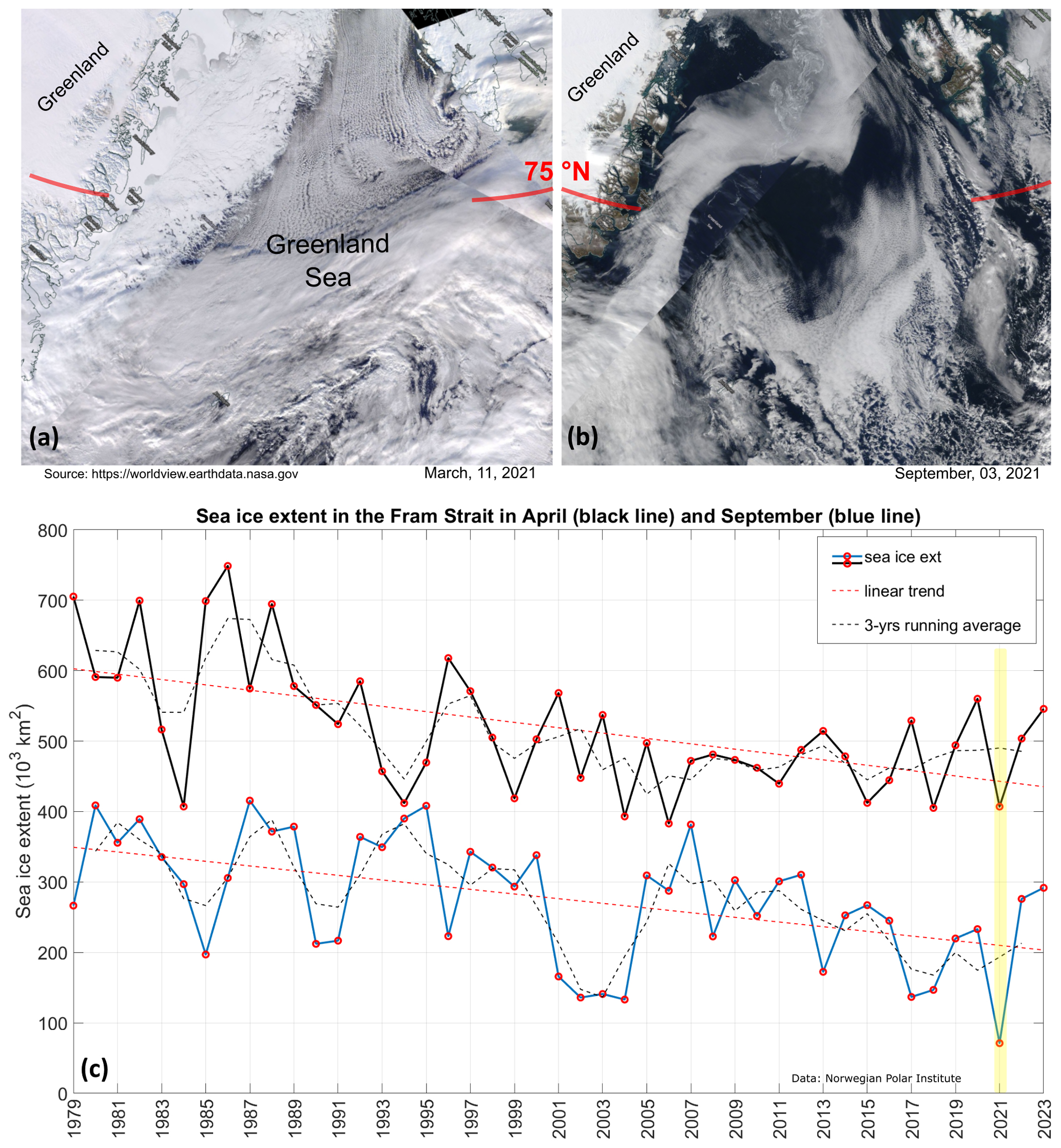
Figure 2 (a, b) Satellite images of the Greenland Sea and the Fram Strait in March and September 2021 (MODIS Corrected Reflectance Imagery, source NASA). (c) April (black line) and September (blue line) mark the annual maximum and minimum sea ice extension in the Fram Strait (source: Norwegian Polar Institute, 2024, Environmental monitoring of Svalbard and Jan Mayen (MOSJ). URL: https://mosj.no/en/indikator/climate/ocean/sea-ice-extent-in-the-barents-sea-and-fram-strait/, last access: 3 June 2025). The yellow vertical bar indicates the year 2021.

3.1 Physical oceanography: thermohaline properties distribution

We grouped our data according to the definition of main water masses from Rudels et al. (1999) and Wang et al. (2021) and adjusted them to include most of our data. Due to some data gaps, it was not possible to define all relevant water masses in this area more precisely. Along the zonal transect at 75° N, the ocean temperature shows a very pronounced horizontal gradient, with typical values of AW (θ>3.0 °C, S>35) in the uppermost 500 m of the water column on the eastern side (Fig. 3). At the surface, the AW has temperatures between 4.5 and 9.0 °C (Fig. 4). The AW extends to the west and gradually becomes shallower, so that from station 20 to station 35 it only occupies the uppermost 50–80 m. In contrast, the surface layer on the western side, from station 38 to station 46, has a thin (about 40–80 m) layer of PW with temperature and salinity values that are typical of sea ice meltwater (θ<0 °C, S≤33). The intermediate zone between 100 m and 500 m is largely occupied by mixed water and we refer to it as the transition layer. The deep layer below 500 m depth is occupied by Greenland Sea Arctic Intermediate Water (GSAIW, −0.9 < θ < 0 °C, S ∼ 34.9) and Greenland Sea Deep Water (GSDW, $\mathit{\theta }<-\mathrm{1.0}$ °C, S < 34.9) in the central and westernmost part, respectively, and Norwegian Sea Deep Water (NSDW, θ ∼ −1.0 °C, S ∼ 34.9) in the easternmost part of the section. We find that the deep layer below 500 m has homogeneous thermohaline properties with a slightly pronounced difference at the easternmost edge where the NSDW flows northwards. The isotherm at 0 °C and the overall distribution of isopycnals (Fig. 3a, c) show a classic dome shape with an upwelling in the central part caused by the effect of the GSG, which tends to lift the intermediate water towards the surface due to its cyclonic (i.e. anticlockwise) sense of rotation. In addition, we are certain that the strong horizontal shear and local meteorological conditions can induce the formation of several mesoscale structures (i.e. eddies, hardly shown by our spatial resolution ranging from about 20 km (along the sides) to 40–60 km (in the centre of the transect). They can change the internal distribution and even trap nutrients and other chemical–biological properties. The dissolved oxygen values show a higher oxygen enrichment (>350 µmol kg⁻¹) in the intermediate layer between stations 15 and 38 (Fig. 3d), while the maximum values are found in the upper layer near the Greenland coasts, where the PW flows southwards. In contrast, lower oxygen values (<300 µmol kg⁻¹) are found below 1500 m depth and in the easternmost part of the section where AW and NSDW occur (Fig. 3d). Turbidity is higher at the surface and along the continental slopes, both on the eastern and western sides, while the fluorescence maximum is at a depth of about 25–30 m, and higher values are found in the easternmost part of the section (Fig. 3e, f). Overall, θ spans from 1.5 °C to almost 9.0 °C, while S spans from 30 (melting waters) to 35 (AW, Fig. 4).

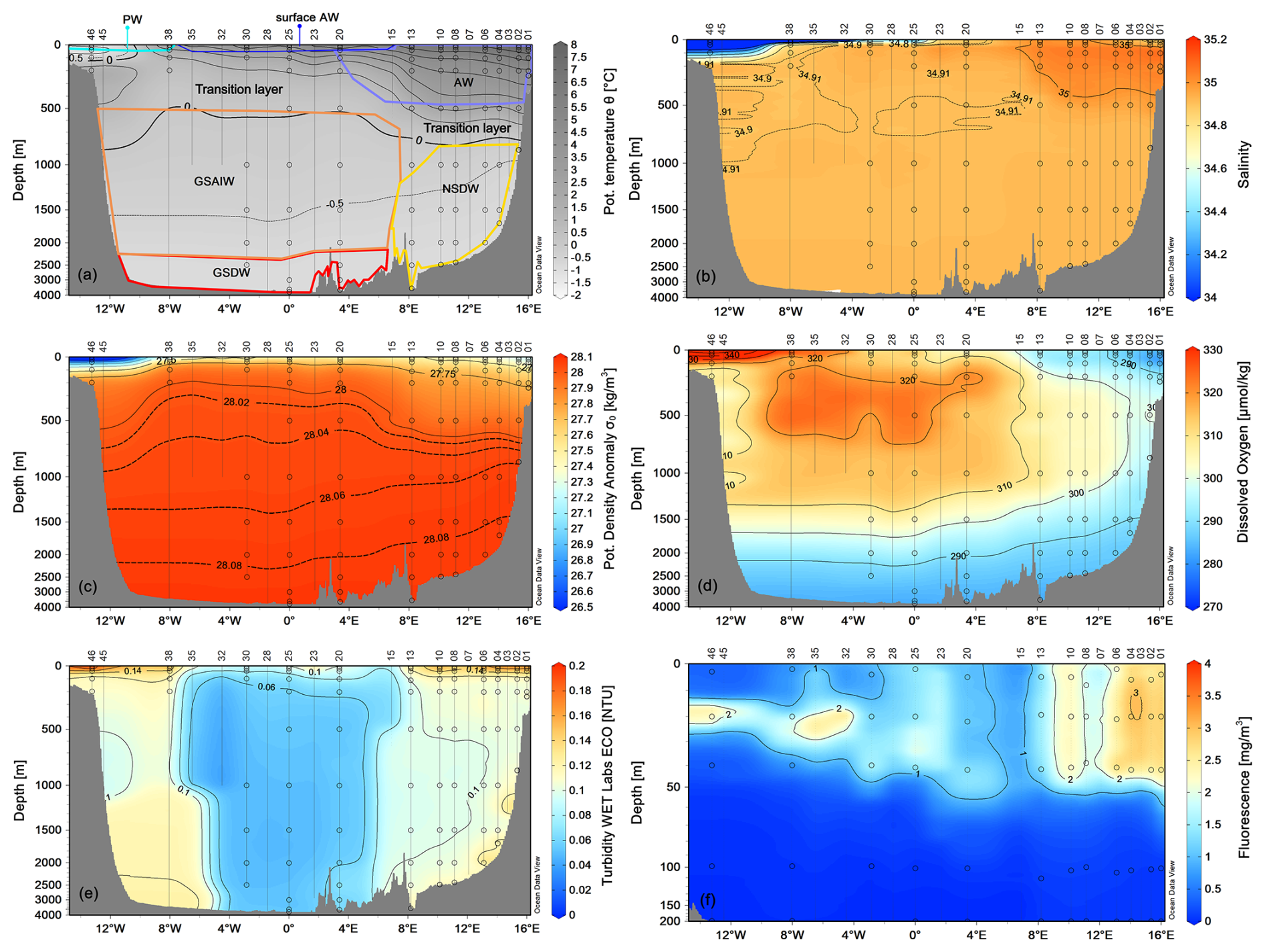
Figure 3 Vertical distribution of (a) potential temperature (°C), (b) salinity, (c) potential density anomaly (kg m⁻³), (d) dissolved oxygen (µmol kg⁻¹), (e) turbidity (NTU), and (f) fluorescence (mg m⁻³) along the zonal transect at 75° N in September 2021. The empty dots indicate the sampling points of the Niskin bottles. Panel (a) also shows the distribution of principal water masses according to their core values (AW – Atlantic Water; GSAIW – Greenland Sea Arctic Intermediate water; NSDW – Norwegian Sea Deep Water; GSDW – Greenland Sea Deep Water; PW – Polar Water or Melting Water). Depths on the y-axis are non-linear. Panels were created with Ocean Data View (Schlitzer, 2024).

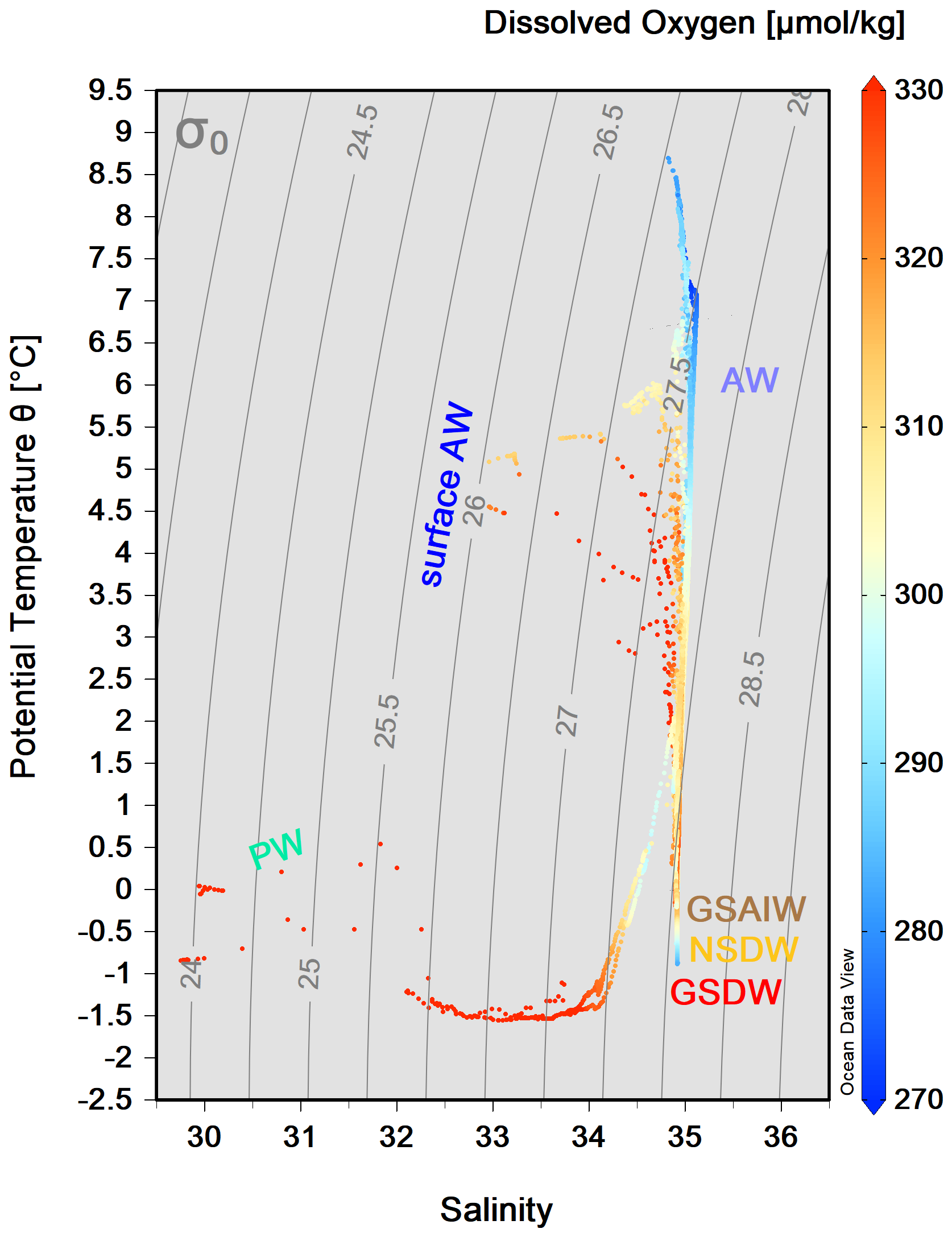
Figure 4 $\mathit{\theta }/S$ diagram from the CTD data collected along the 75° N section during the LB21 cruise in September 2021. The colour bar on the right-hand side refers to the values for dissolved oxygen concentration (µmol kg⁻¹). (For water mass acronyms, see the caption of Fig. 3.) The figure was created with Ocean Data View (Schlitzer, 2024).

3.2 Biogeochemistry

Along the entire transect, except for the two edges, the seasonal warming in summer had created a well-stratified upper layer about 30–50 m deep. At the surface, the central Greenland Sea appears to be almost nutrient poor (Fig. 5). The western side of the transect is characterised by higher concentrations of phosphate and silicate, good indicators of the upper halocline of Arctic surface water along the Greenland slope, whereas nitrate concentrations are very low. At depth, NSDW and GSDW (see Figs. 3 and 5) were enriched with silicate.

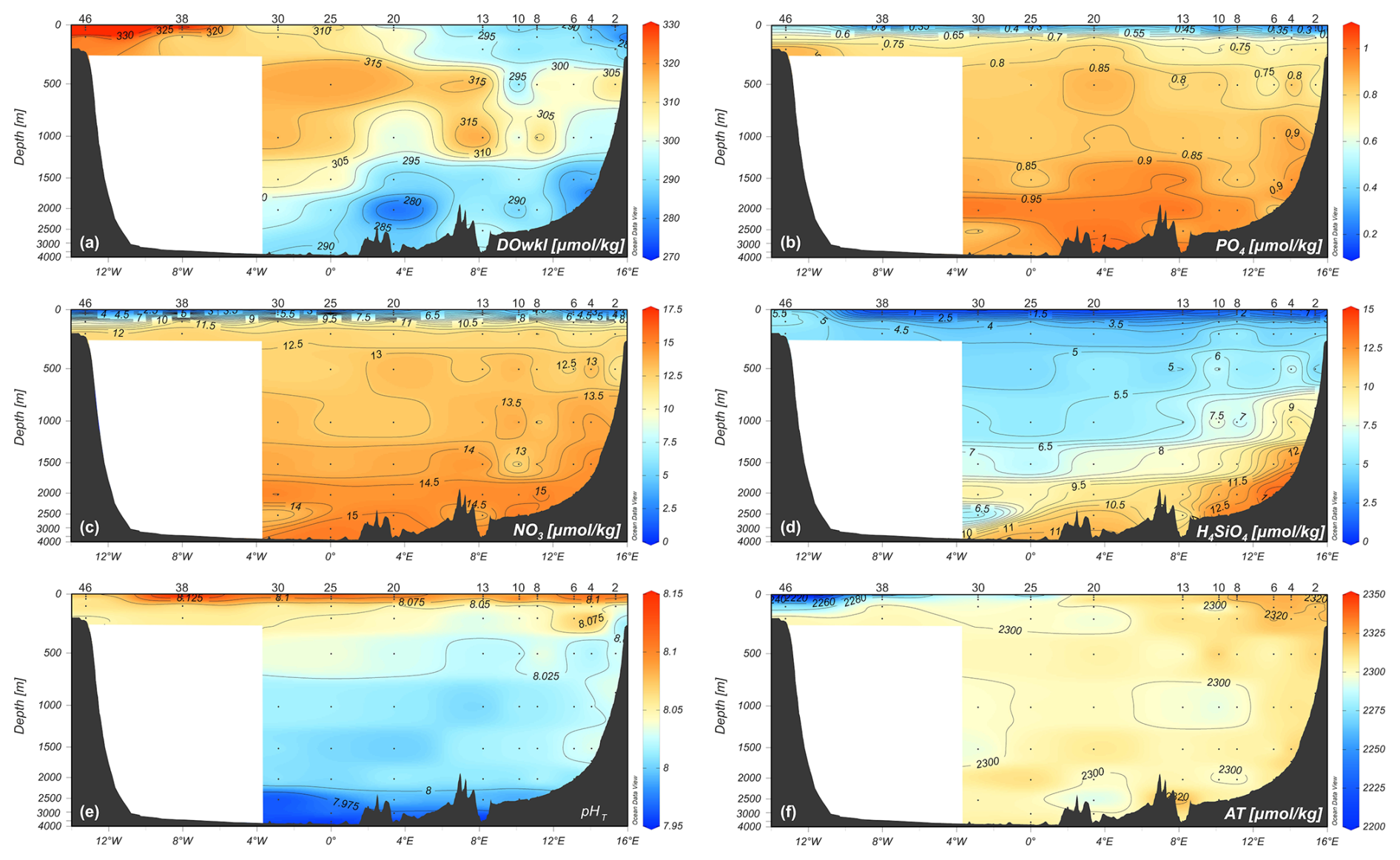
Figure 5 Vertical distribution of (a) dissolved oxygen concentration (µmol kg⁻¹), (b, c, d) nutrients concentration (µmol kg⁻¹), (e) pH_T, and (f) total alkalinity (µmol kg⁻¹) along the zonal transect at 75° N during the LB21 cruise in September 2021. Data are obtained from the laboratory analyses on water samples. Depths on the y-axis are non-linear. Panels created with Ocean Data View (Schlitzer, 2024).

A marked vertical gradient is found along the entire transect with higher pH_T values (up to 8.227, Fig. 5e) in the photic layer (<100 m depth) decreasing with increasing depth and reaching the lowest values (7.946–7.997) in the deep layer of the Greenland Sea, presumably due to the degradation of settling organic matter. High total alkalinity values (Fig. 5f) are found on the easternmost side where the AW and NSDW flow northwards. The highest values (A_T up to 2320–2348 µmol kg⁻¹) are found in the higher salinity AW and particularly in the photic layer also due to the contribution of photosynthetic activity. The lowest values are instead associated with fresh PW found at the surface on the westernmost part of the section.

At the surface layer, a high variability in the organic matter pool (POC and DOC) is observed (Fig. 6); a decreasing trend down to 1000 m depth and an increase towards greater depths characterise the vertical profiles of DOC. POC concentrations range from 11.2 µg C L⁻¹ (station 30, at 2002 m depth; 0.93 µM C) to 160 µg C L⁻¹ (station 46, at 198 m depth; 13.3 µM C). A greater variability with depth is observed (coefficient of variation higher than 65). The highest values are generally found at the surface and within the depth interval of 20–40 m. The highest (mean) concentration is measured at station 46 (80.5 ± 53.4 µg C L⁻¹), while slightly lower (mean) values are found at stations 1, 30, and 38 (67.2 ± 46.8, 41.0 ± 23.1, and 60.0 ± 15.3 µg C L⁻¹, respectively), and the lowest values are found at stations 10 and 20 (34.1 ± 31.0 and 28.2 ± 20.5 µg C L⁻¹, respectively). DOC shows classic vertical profiles, with the highest concentrations (1.22 mg C L⁻¹; 101.7 µM C) at station 30 (20 m depth) and a decrease to a minimum of 0.5 mg C L⁻¹ (41.7 µM C) at station 10 (499 m depth). Between 200 and 1000 m depth, the values remain low (mean 0.83 ± 0.22 mg C L⁻¹; 69.2 ± 18.3 µM C), while a slight increase was observed in the bottom water, particularly at stations 20 and 10 (Fig. 6).

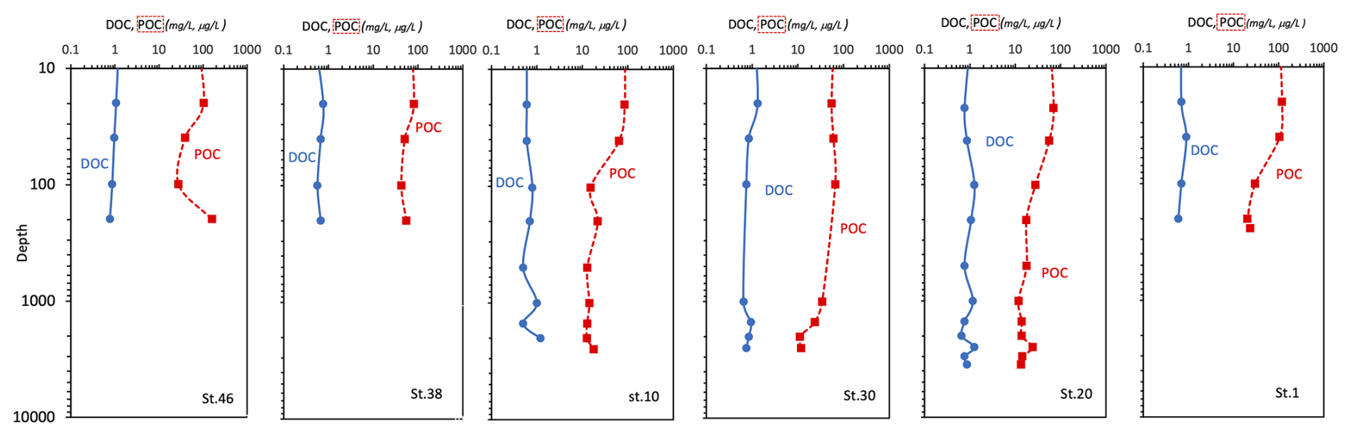
Figure 6 Vertical profiles of dissolved organic carbon (DOC, mg L⁻¹) and particulate organic carbon (POC, µg L⁻¹) concentrations; data are represented in natural log (ln) scale.

The isotope values in the total of 96 analysed samples range from −0.43 ‰ to 0.8 ‰ for δ¹⁸O and from −2.51 ‰ to 5.36 ‰ for δD. Along the transect, a gradient from west to east can be seen in the surface waters, with lower values for δ¹⁸O and δD on the westernmost side (Fig. 7). The lowest values at the surface in the westernmost part of the section could be related to fresh PW, while the higher values in the easternmost part could be related to northward-flowing AW. At depths between 500 m and 1000 m, isotope values drop to a relative minimum, while maxima occur near the bottom at stations 20 and 25, where GSDW is identified. In addition, a minimum is observed at depth at stations 8 and 10, in an area occupied by NSDW.

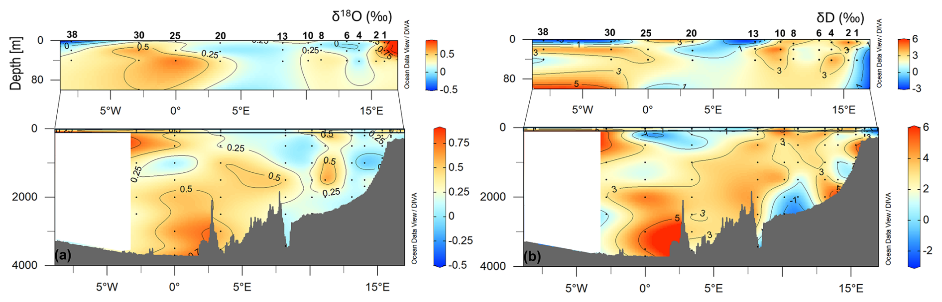
Figure 7 Vertical distribution of δ¹⁸O (a) and δD (b) along the zonal transect at 75° N during the LB21 cruise in September 2021. Panels were created with Ocean Data View (Schlitzer, 2024).

3.3 Phytoplankton

3.3.1 Total and size-fractionated chlorophyll a (chl-a)

Integrated total chl-a in the euphotic layer (0–100 m) averages 55.4 mg m⁻², while the highest concentrations (73.1 mg m⁻²) are found at stations located at the ends of the transect (65.3 mg m⁻²) close to the continental shelf (Fig. 8). The concentration of chl-a at different depths ranges between 0.20 mg m⁻³ (station 1, 100 m) and 2.90 mg m⁻³ (station 1, 20 m) with an average value of 0.63 ± 0.64 mg m⁻³. Degraded pigments (phaeo) are around 40 % with respect to chl-a. The size spectrum of the phytoplankton community biomass along the water column shows different percentage contributions to the total, with 65 % for the nano-phytoplankton, 21 % for the micro-phytoplankton, and 14 % for the pico-phytoplankton (Fig. 8). Exception to this composition is observed in the westernmost station (station 46) where the micro-fraction dominates, replacing the nano-phytoplankton.

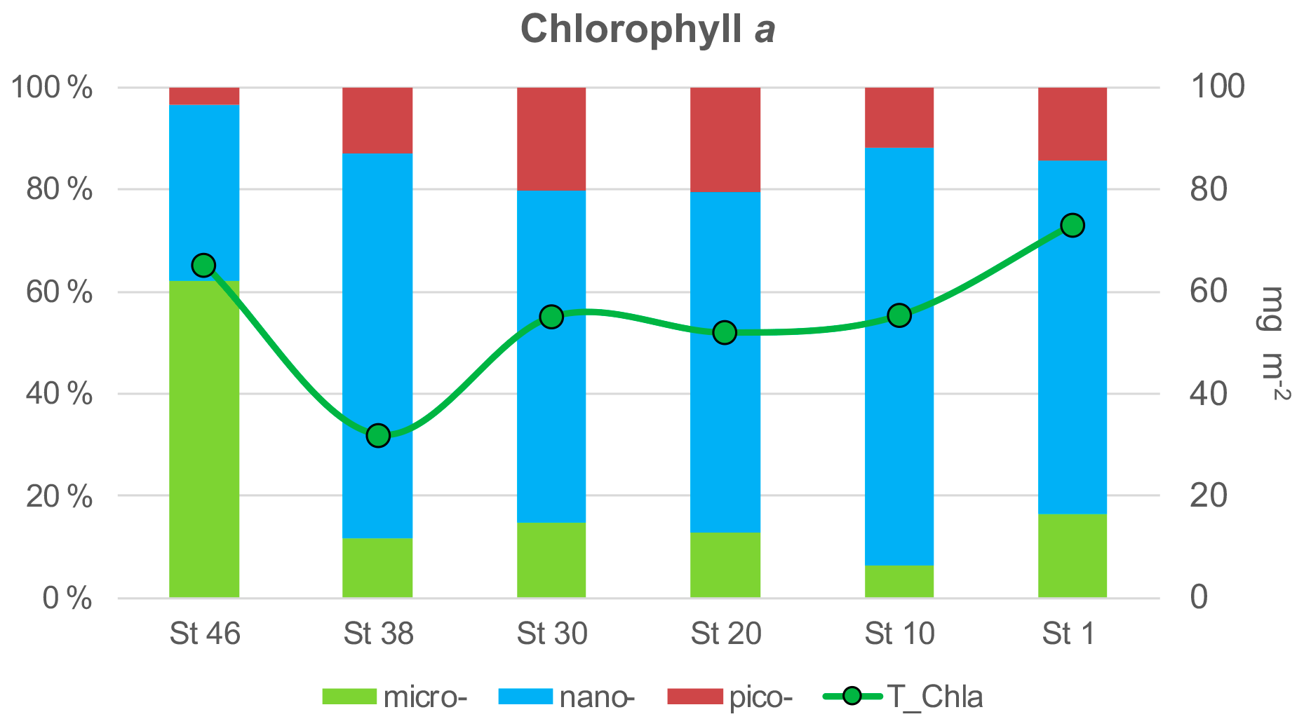
Figure 8 Integrated total chl-a concentration (0–100 m depth) at the stations along the 75° N zonal transect (green line) with the percentage of contribution of micro-, nano-, and pico-phytoplankton size fractions (histogram).

3.3.2 Phytoplankton composition and abundances

The phytoplankton analyses do not reveal a clear pattern along the transect, although some differences in abundance and composition were observed. The integrated abundances of phytoplankton, ranging from 7.00 (station 30) to 23.48×10⁴ cells L⁻¹ (station 20), are higher at the easternmost stations than at the westernmost ones (on average 19.33×10⁴ cells L⁻¹ at stations 1, 10, and 20 and 9.44×10⁴ cells L⁻¹ at stations 30, 38, and 46; see Fig. 9). This is mainly due to a more even vertical distribution of abundance at the eastern stations. In contrast, the westernmost stations have even higher phytoplankton abundances, but limited to subsurface maxima, like 50.40×10⁴ cells L⁻¹ at 38 m at station 20, while abundances in the rest of the water column are very low. The phytoplankton community along the transect is characterised by the dominance of the flagellate group (70 % of the total phytoplankton), mainly represented by small (<10 µm) forms with uncertain taxonomic identification (on average, 61 %). Diatoms (on average, 9 % of the total phytoplankton) are present in very low abundances in the easternmost and central stations (on average, 0.43×10⁴ cells L⁻¹ at stations 1, 10, 20, and 30), while higher values were recorded in the two westernmost stations 38 and 46 (on average, 3.24×10⁴ cells L⁻¹). Finally, dinoflagellates accounted for an average of 21 % of the total phytoplankton, with higher abundances occurring in the easternmost stations than in the westernmost stations (3.32×10⁴ and 1.42×10⁴ cells L⁻¹, respectively).

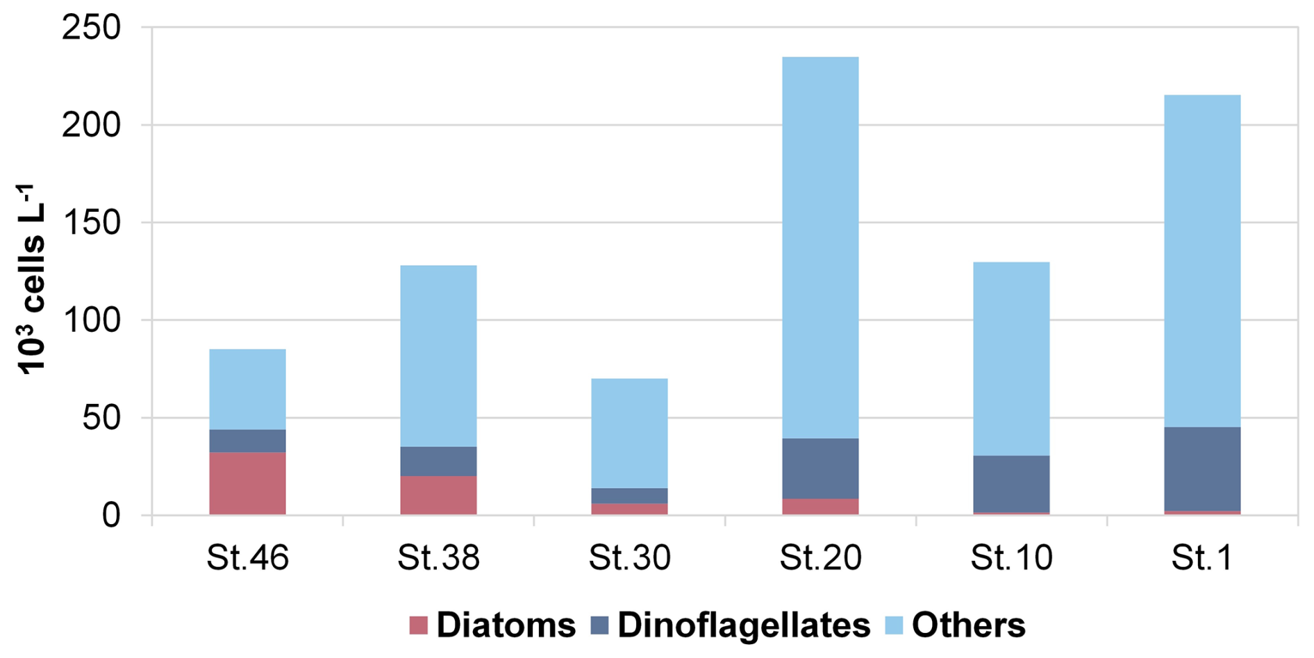
Figure 9 Integrated values (0–100 m) of abundance (cell L⁻¹) of the main phytoplankton groups (diatoms, dinoflagellates, and others) at the sampled stations along the 75° N transect.

3.4 Zooplankton

3.4.1 Microzooplankton abundance and biomass

The MZP abundance in the study area varies between 721.5 ind. L⁻¹ (station 38, at 0 m) and 6.25 ind. L⁻¹ (station 20, at 3500 m). The carbon content shows higher values at the surface with a maximum value of 1.7 µgC L⁻¹ (station 38, 0 m) and a minimum of 0.01 µgC L⁻¹ at 2520 m depth (station 10). The vertical distribution of organisms, based on their abundance along the water column, shows higher abundances in the first 200 m compared to the zone >200 m. In particular, the integrated abundance of MZP in the upper layer reaches its maximum at station 38, mainly due to the higher presence of tintinnids, while the lowest values are found at station 20, in the centre of the transect (Fig. 10). The highest carbon content is recorded at station 10, which is due to the high abundance of other protists and micrometazoans (Fig. 10). Tintinnids are the most abundant taxa in the study area, followed by heterotrophic dinoflagellates and aloricate ciliates (Fig. 10).

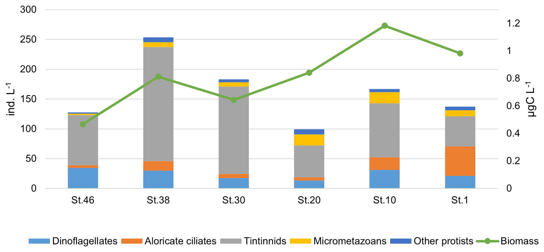
Figure 10 Integrated values (0–200 m) of abundance (ind. L⁻¹) and biomass (µgC L⁻¹) of microzooplankton groups (dinoflagellates, aloricate ciliates, tintinnids, micrometazoans, and other protists) at the sampled stations along the 75° N transect.

3.4.2 Mesozooplankton biomass and abundance

Biomass and abundance of mesozooplankton have the same distribution along the transect both at the surface (ca. 20 cm depth, Fig. 11a) and in the upper layer (0–100 m depth, Fig. 11b), with the highest values found in the central part of the transect (station 20). Nevertheless, the surface samples are richer in organisms than those collected in the water column (mean abundance: Manta net: 1257 ± 1110 ind. m⁻³; WP2 net: 492 ± 387 ind. m⁻³), which also corresponds to a higher biomass (mean biomass: Manta net: 41 ± 32 mg DM m⁻³; WP2 net: 10 ± 7 mg DM m⁻³). Overall, organisms 1–2 mm in size account for 61 % of the mesozooplanktonic biomass in the surface waters and are the most abundant at almost all stations (Fig. 11a), while in the samples collected with the WP2 net, the biomass fractions consisting of organisms 1–2 mm and >2 mm in size were the most abundant, accounting for 35 % and 38 % of the total biomass, respectively (Fig. 11b). Copepods are the most abundant taxon both at the surface and in the upper layer (97 % and 94 % of the total mesozooplankton abundance, respectively), mainly represented by the genus Calanus. Chaetognaths, although much less abundant than copepods, are found along the entire transect both at the surface and in the upper layer, being most numerous at stations 10, 20, and 30. Molluscs are almost absent in the surface water and are mainly found in the water column at the eastern stations of the transect (station 1 and station 10).

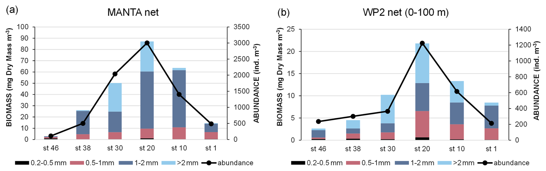
Figure 11 Biomass and abundance of mesozooplankton: (a) Manta net sampling at surface and (b) WP2 net sampling in the 0–100 m layer.

3.5 Microbial compartment: abundance, biomass, and activities

The abundance of prokaryotes is high in the photic (0–100 m depth) layer (range: 5.57×10⁵ to 11.3×10⁵ cells m⁻³) and decreases with depth. The highest values are measured at stations 20 and 1. From 100 m to 1000 m depth, the abundance ranges from 1.75×10⁵ to 3.21×10⁵ cells m⁻³ and from 0.53×10⁵ to 0.64×10⁵ cells m⁻³ at greater depths. The cell volume ranges from 0.049 to 0.098 µm³ with a mean value of 0.072 ± 0.018 µm³. In the photic and aphotic layers, the cell volumes vary in a similar range (0.08±0.02 µm³). The highest volumes at great depths characterise stations 30 and 10, where large, curved rods are observed. Apart from stations 30 and 10, data show a similar vertical profile in the size distribution. The highest percentage of live cells (about 33 %) is observed at station 46 in the photic layer. However, peaks are also found in the deeper layers. The number of respiring cells (CTC+) is in the order of 104 cells mL⁻¹. Variability between the layers is observed at all stations. In general, the high proportion of respiring cells below 100 m depth is observed at stations 46, 30, and 20. Conversely, the higher percentages are found in the photic layer at stations 10 and 1 (Fig. 12).

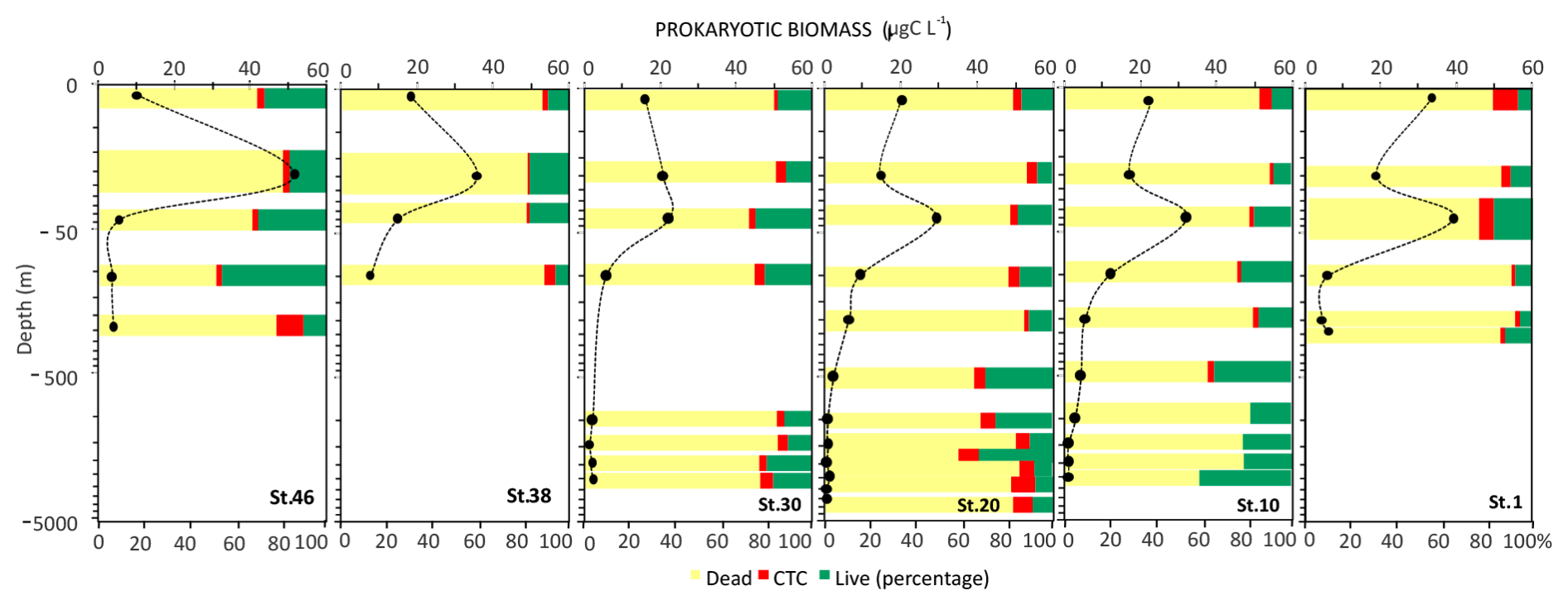
Figure 12 Vertical profiles of prokaryotic biomass, viable and dead cells (Live/Dead) and respiring cells (CTC). Data on the y axis are represented in natural log (ln) scale.

Overall, the average percentages of carbon source utilisation determined by Biolog EcoPlates show that carbohydrates and carboxylic acids were well-utilised polymers at each station and in each layer. Especially in the aphotic layer, these polymers showed the highest percentage utilisation at most stations. Complex carbon sources and phosphate carbon are utilised at similar percentages throughout the water column; conversely, amino acids are preferentially utilised in the aphotic layer. Amines are only little used (Fig. 13).

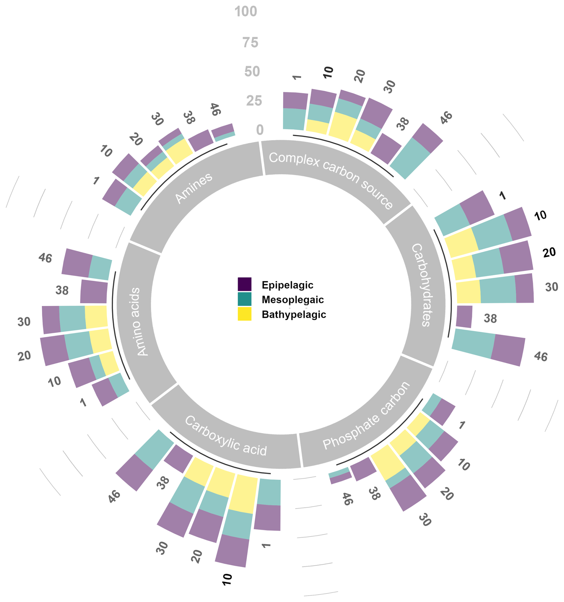
Figure 13 Carbon substrate utilisation (as percentage of the total) determined in the epi-, meso-, and bathy-pelagic layers.

Enzymatic activity measurements yield values of LAP, GLU, and AP ranging from 0.072 to 8.08 nM h⁻¹, from 0.007 to 0.35 nM h⁻¹, and from 0.001 to 0.36 nM h⁻¹, respectively (Fig. 14). Total enzymatic patterns depict vertical trends generally decreasing from surface towards deep layers, with some hotspots of metabolic activity at 20–40 m and in the aphotic layer. LAP activity peaks at the lateral ends of the transect as well as at station 20. AP and GLU decrease from the western (Greenland) side moving towards station 20, then increase again towards the eastern side (station 10) of the transect.

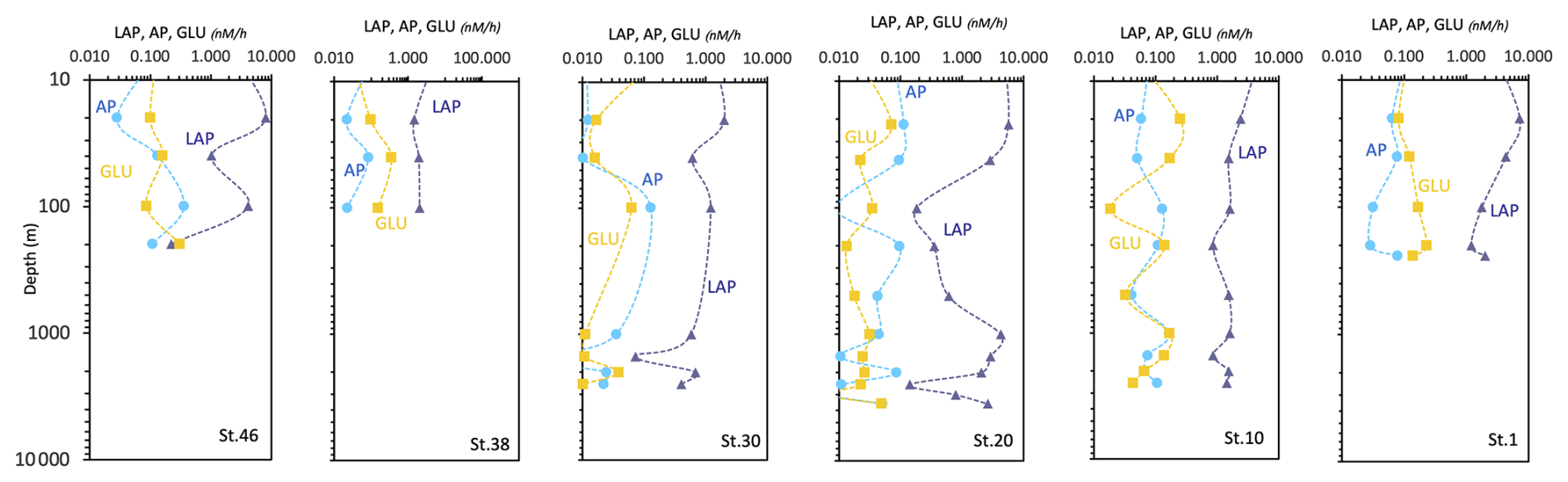
Figure 14 Vertical profiles of the enzymatic activity rates measured at the sampled stations (LAP, leucine aminopeptidase; AP, alkaline phosphatase; GLU, beta glucosidase). Data are represented in natural log (ln) scale.

The respiration rates (ETS) range from 0.0290 to 0.329 µL O₂ h⁻¹ L⁻¹ (Fig. 15). The respiratory activity values generally decrease from the surface down to 1000 m depth and then increase again in the deep layer (below 1000 m depth). A high value of respiratory activity was also determined in the deepest sample of station 46.

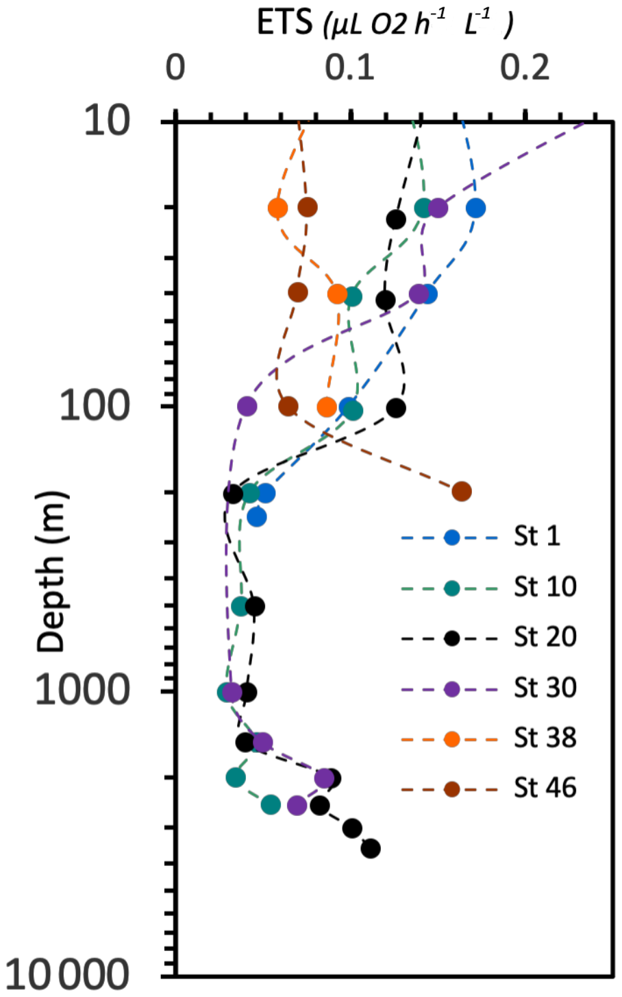
Figure 15 Vertical profiles of electron transport system (ETS) respiratory activity. Data on the y axis are represented in natural log (ln) scale.

4 Data availability

Data presented here are available through the repository Italian Arctic Data Center (IADC), at the following links. CTD casts are available at https://doi.org/10.71761/c082c3ca-40bf-42b1-a61a-7b3697ab2c5a (Bensi et al., 2024). Physical, biological, and biogeochemical analyses on water samples from Niskin bottles are available at https://doi.org/10.71761/f7474404-3331-43e5-883b-25755e94956d (Azzaro et al., 2024). Satellite data used in this work and data on sea ice extension are freely available (see Fig. 2).

5 Summary and conclusions

Here we present the main data and results of the multidisciplinary oceanographic campaign carried out between 29 August and 14 September 2021 on board the Italian icebreaker Laura Bassi in the Greenland Sea (along the 75° N latitude section) as part of the Italian project CASSANDRA, funded by the Italian Ministry of Research in the framework of the Italian Arctic Programme. The Greenland Sea, in the north Atlantic, is a region of deep ocean convection that contributes to the AMOC and the exchange of water masses between the Atlantic and Arctic Oceans. On its easternmost side, it is dominated by the presence of AW, while on the westernmost side, by the presence of Polar waters. Large-scale patterns, local meteorological conditions, and ice extent can all influence physical and biogeochemical properties. Different phases of the North Atlantic Oscillation index (NAO, i.e. atmospheric pressure difference between the Azores high and the subpolar low at sea level) can modulate basin-wide changes in the intensity and position of the North Atlantic jet stream and storm track, as well as influence patterns of zonal and meridional heat and moisture transport, which in turn can affect temperature and precipitation patterns over the Arctic and sub-Arctic regions. Increasingly positive phases of the NAO are associated with increased AW inflow, as was the case in the late 1980s/early 1990s (Dickson et al., 2000). The winter of 2020/2021, which preceded the cruise, had a slightly negative NAO index (−0.72), after 2 years of predominantly positive values. A negative NAO means weaker westerly winds in the mid-latitude regions in terms of climatology and stronger winds in the North Atlantic west of Iceland. Sea ice in the Fram Strait fluctuates from year to year. The lowest extent in September was recorded exactly in 2021, the highest in 1987. In the long term, the regions of the Norwegian Sea and the Fram Strait experienced a drop in temperature from 2018 to 2020, which rose again in 2021. Instead, a strong freshening phase set in after 2013, which is continuing. Continuous warming was also observed in the deep-water layer of the Greenland Sea at a depth of 3000 m. In particular, the GSDW temperature shows a relatively steady increase from −1.18 °C to −0.86 °C between 1993 and 2021 (ICES Report on Ocean Climate 2021, available at https://ices-library.figshare.com/articles/report/ICES_Report_on_Ocean_Climate_2021/24755574?file=43769571, last access: 8 May 2025). Our measurements report temperature values of about −0.9 °C for the GSDW. Relatively warm and saline Atlantic Water (AW, θ > 3.0 °C, S about 35), with highest A_T concentrations, dominates on the eastern side in the upper 500 m with surface temperatures of 4.5–9.0 °C. A dome-shaped isotherm distribution indicates upwelling from the Greenland Sea Gyre, while several mesoscale structures such as eddies seem to be responsible for the large spatial variability in the upper layer. At the surface, the central Greenland Sea is almost nutrient poor. On the western side, however, higher phosphate and silicate values are good indicators for the upper halocline of the Arctic surface water along the Greenland slope. Nitrate levels remained very low there. The deep waters NSDW and GSDW presented the lowest pH_T values and the highest enrichment of silicate. Phytoplankton biomass along the euphotic water column, expressed as chl-a, showed a difference between the central-eastern and western sectors with greater abundances at the extremes of the transect. The dimensional structure of the phytoplankton community characterises the PW with a predominance of the micro-phytoplankton fraction that almost entirely replaces the nano-phytoplankton fraction, more abundant in the AW, even in the front station between these two water masses. The plankton communities were analysed with more detail in the upper layer (0–100 m), where the phytoplankton and zooplankton diversity reflected the different water masses (AW and PW). Diatoms increased at the western stations affected by PW, while dinoflagellates and small flagellates were more abundant at the eastern stations affected by AW. The higher MZP abundance was recorded at station 38, where the layer below 30–40 m depth was still occupied by AW, while the surface layer was affected by PW. The MZP abundance and biomass decreased drastically in the presence of cold PW on the Greenland slope. Micrometazoans and aloricate ciliates increased towards the easternmost side of the section, where the stations were characterised by higher sea temperatures. Copepods of the genus Calanus were the main taxa observed, but the structure of the mesozooplankton communities changed along the transect and polar taxa increased westwards. The δ¹⁸O and δD isotope ratios indicate the influence of freshwater at the surface level near the Greenland shelf. We also highlight a marked difference in δ¹⁸O and δD isotope ratios between GSDW and NSDW, which occupies the bottom region of the studied area, with NSDW showing lower values compared to GSDW. Prokaryotic abundance and microbial enzymes generally depicted vertical decreasing trends with peaks of cells and activity recorded at station 20 as well as at the ends of the transect. While living cells prevailed at station 46 in the photic layer, actively respiring cells were quite variable in their distribution. Large, curved rods were found at stations 30 and 10. A high utilisation of carbohydrates and carboxylic acids regardless of the examined station or depth characterised the microbial community metabolism. Amino acids were actively metabolised in the aphotic layer, while no differences were found in the utilisation of complex carbon sources and phosphate carbon compounds along the water column.

This study emphasises the significant spatial and vertical variability of water properties, nutrient distribution, and biological communities caused by local and seasonal oceanographic dynamics in a region characterised by a strong exchange of water masses between the Arctic and Atlantic Oceans and a major influence of atmospheric teleconnections between the polar and subpolar regions.