Multi-temporal high-resolution data products of ecosystem structure derived from country-wide airborne laser scanning surveys of the Netherlands

Recent years have seen a rapid surge in the use of light detection and ranging (lidar) technology for characterizing the structure of ecosystems. Even though repeated airborne laser scanning (ALS) surveys are becoming increasingly available across several European countries, so far, only a few studies have derived data products of ecosystem structure at a national scale, possibly due to a lack of free and open-source tools and the computational challenges involved in handling the large volumes of data. Nevertheless, high-resolution data products of ecosystem structure generated from multi-temporal country-wide ALS datasets are urgently needed if we are to integrate such information into biodiversity and ecosystem science. By employing a recently developed, open-source, high-throughput workflow (named “Laserfarm”), we processed around 70 TB of raw point clouds collected from four national ALS surveys of the Netherlands (AHN1–AHN4, 1996–2022). This resulted in ∼59 GB raster layers in GeoTIFF format constituting ready-to-use multi-temporal data products of ecosystem structure at a national scale. For each AHN (Actueel Hoogtebestand Nederland) dataset, we generated 25 lidar-derived vegetation metrics at 10 m spatial resolution, representing vegetation height, vegetation cover, and vegetation structural variability, together with auxiliary data (∼12 GB) such as raster layers of point density; pulse density; flight line timestamp information; terrain and surface elevation; and masks of water areas, roads, buildings, power lines, and NA values (areas with no points available). The data enable an in-depth understanding of ecosystem structure at a fine resolution across the Netherlands and provide opportunities for exploring ecosystem structural dynamics over time. To illustrate the utility of these data products, we present ecological use cases that monitor forest structural change and analyse vegetation structure differences across various Natura 2000 habitat types, including dunes, marshes, grasslands, shrublands, and woodlands. The provided data products and the employed workflow can facilitate a wide use and uptake of ecosystem structure information in biodiversity and carbon modelling, conservation science, and ecosystem management. The full data products are publicly available on Zenodo (https://doi.org/10.5281/zenodo.13940846, Shi et al., 2025a).

1 Introduction

Monitoring ecosystem structure is essential for sustainable forest management (Lindenmayer et al., 2000), species distribution research (Jetz et al., 2019; Kissling et al., 2018), dynamic ecosystem modelling (Kucharik et al., 2000), biodiversity monitoring (Noss, 1990), and the conservation and restoration of terrestrial ecosystems (Ruiz-Jaén and Aide, 2005). As one of the classes of Essential Biodiversity Variables (EBVs) (Pereira et al., 2013), ecosystem structure provides detailed insights into both the vertical and horizontal profiles of ecosystems, facilitating a deeper understanding of the relationship between vegetation structure and animal ecology (Davies and Asner, 2014), forest attribute modelling (Coops et al., 2021), and carbon and biomass dynamics (Zhao et al., 2018; Dalponte et al., 2019). However, until a decade ago, the collection of vegetation structure data was difficult and labour intensive, especially over large spatial extents. Although previous studies have explored the use of passive remote sensing technologies, such as high-resolution satellite imagery and aerial photographs alongside field measurements to obtain structural information (e.g. Wolter et al., 2009; Lamonaca et al., 2008), these applications have largely been confined to plot or local scales, with limited scalability and uncertain transferability between different regions.

Over the past few decades, the advent of airborne laser scanning has enabled precise and spatially contiguous measurements of ecosystem structural properties such as high-resolution topographic variation and accurate estimation of vegetation height, cover, and canopy structure (Lefsky et al., 2002). The lidar technology used in airborne laser scanning (ALS) surveys generates discrete returns (point clouds) and/or full-waveform signals by emitting laser pulses from the sensor towards the target objects (e.g. ground, trees, and buildings), recording the distance between the sensor and the objects (“X”, “Y”, “Z” coordinates), the amount of energy returned to the sensor (“intensity”), the sequence of returns generated from one pulse (“return number” and “number of returns”), the time at which the objects were observed (“GPS time”), and so on. Advances in sensor systems and techniques also allow many countries to carry out ALS campaigns over national or regional extents, producing fine-scale ecosystem measurements across broad spatial extents (Kissling et al., 2022; Assmann et al., 2022). ALS surveys often generate massive amounts of data (e.g. point clouds with a multi-terabyte data volume) which contain ecosystem structural information that is essential for ecological and biodiversity research (Kissling et al., 2022; Koma et al., 2021b; Bakx et al., 2019). Although tools and software for processing large amounts of lidar data are becoming increasingly available (Roussel et al., 2020; Isenburg, 2017; Meijer et al., 2020; Kissling et al., 2022; Fischer et al., 2024), significant challenges remain, including the need for specialist expertise, extensive data storage, and substantial computational power (Assmann et al., 2022). Ultimately, ecologists, foresters, biodiversity researchers, and land managers require raster layers with vegetation structural information that can be readily integrated into analytical workflows using software that they are familiar with (e.g. GIS, R, Python). Such raster layers, e.g. lidar-derived vegetation metrics, are often generated by statistically aggregating the 3D point cloud information within spatial units such as voxels or 2D raster cells (Meijer et al., 2020; Kissling et al., 2022; Fischer et al., 2024). These lidar-derived vegetation metrics typically capture three key dimensions of ecosystem structure: vegetation height (e.g. maximum vegetation height, vegetation height at a certain percentile), vegetation cover (e.g. the density of vegetation at a given height layer), and vegetation structural variability (e.g. the vertical or horizontal distribution and variability of vegetation within a spatial unit) (Kissling et al., 2023; Bakx et al., 2019). Providing high-resolution (e.g. 10 m) ready-to-use lidar metrics and making them accessible to the public are thus critical for monitoring Essential Biodiversity Variables (EBVs) (Valbuena et al., 2020), modelling species distributions (de Vries et al., 2021; Koma et al., 2021b; Zellweger et al., 2013), and estimating species diversity (Moeslund et al., 2019; Zellweger et al., 2017; Aguirre-Gutiérrez et al., 2017) at a regional or national scale.

Ecosystem structure is a three-dimensional phenomenon with horizontal and vertical components that change over time (Zenner and Hibbs, 2000). The increasing frequency of ALS data acquisition offers a unique opportunity to monitor ecological changes and ecosystem dynamics at fine spatial and temporal scales. Several countries have been conducting repeated (sub-)national ALS surveys to obtain fine-scale information on topography and forest ecosystems (Nilsson et al., 2017). For example, the Dutch national ALS programme (AHN, Actueel Hoogtebestand Nederland, https://www.ahn.nl/, last access: 24 July 2025) has been collecting country-wide lidar data since 1996, providing four complete ALS datasets (AHN1–AHN4), with an ongoing fifth survey (AHN5), conducted at intervals of 3 to 5 years. In Spain, under the PNOA-LiDAR project, two national ALS campaigns took place during 2008–2015 (lidar first coverage) and during 2015–2021 (lidar second coverage), while the third acquisition (lidar third coverage) started in 2023 and is planned to finish in 2025 (https://centrodedescargas.cnig.es/CentroDescargas/modelos-digitales-elevaciones, last access: 24 July 2025). While the primary goal of many ALS campaigns is to produce terrain and surface elevation models, such as digital terrain models (DTMs) and digital surface models (DSMs), the multi-temporal lidar datasets also capture detailed 3D characteristics of vegetation structure over time, providing valuable information for evaluating changes in biomass (Cao et al., 2016; Feng et al., 2024), forest structure (McCarley et al., 2017; Riofrío et al., 2022; Vepakomma et al., 2011), and forest carbon stocks (Dalponte et al., 2019; Zhao et al., 2018). Furthermore, these datasets are increasingly being integrated with other remote sensing data, such as satellite imageries from Landsat, Sentinel-2, and synthetic aperture radar (SAR), to assess forest changes caused by disturbances like wildfires (Li et al., 2023; Feng et al., 2024) and to model aboveground biomass (Musthafa and Singh, 2022). However, despite the growing availability of multi-temporal ALS datasets, there is a noticeable lack of publicly available data products, i.e. lidar-derived vegetation metrics, from national ALS surveys.

Several challenges emerge when generating accurate and standardized data products from multi-temporal ALS data (Valbuena et al., 2020). Over the last 3 decades, advances in lidar sensors and associated technologies have led to improvements in point density, classification accuracy, and additional attributes provided in each point (Riofrío et al., 2022). However, these advancements also introduce complexities into data harmonization. In addition to the challenges associated with processing large datasets and high computational costs (Meijer et al., 2020), discrepancies in sensor technology and flight configurations across different ALS surveys can hinder the generation of consistent data products (Lin et al., 2022). For instance, the first Dutch national ALS campaign (AHN1, 1996–2003) had an average point density ranging from 1 point per 16 m² to 1 point m⁻², with no detailed point classification available. By contrast, in the fourth campaign (AHN4, 2020–2022), the point density improved to 20–30 points m⁻², with a detailed classification code being provided for each point following the ASPRS standard (ASPRS, 2019). These technological variations inevitably result in data products with varying quality and accuracy, introducing uncertainties with regard to their usability (Tompalski et al., 2021; Hopkinson et al., 2008). To understand ecosystem dynamics accurately, changes detected from multi-temporal ALS datasets should reflect actual ecological changes in the target of interest rather than differences in data acquisition or quality (Riofrío et al., 2022). Identifying the limitations and providing usage notes of derived data products are important for users to interpret the data products correctly and to apply them optimally in their analyses.

Here, we present a new set of multi-temporal data products of ecosystem structure derived from four national ALS surveys of the Netherlands (AHN1–AHN4). The data products, with a spatial resolution of 10 m, include four sets of 25 lidar-derived vegetation metrics representing vegetation height, vegetation cover, and vegetation structural variability, aimed at supporting a wide range of ecological applications. In this paper, we (1) describe the ALS data collection from AHN1–AHN4 and the employed “Laserfarm” workflow used to generate the data products; (2) present the detailed characteristics of the generated multi-temporal data products (i.e. lidar-derived vegetation metrics as GeoTIFF raster layers) and their known limitations and corresponding usage notes; (3) provide auxiliary data (e.g. raster layers of point density, pulse density, flight line timestamp information, DTMs, DSMs, and mask layers of water areas, roads, buildings, power lines, and NA values (areas with no points available) to facilitate multi-temporal comparisons) to facilitate multi-temporal comparisons; (4) demonstrate two use cases for using the generated data products in ecological applications; and (5) discuss the potential use of these data products and recommendations for utilizing these data products in future research. Note that the AHN1 dataset has a rather poor quality, which limits its use for ecological applications. To facilitate open science, we make the data products, employed workflow, Python script, and related documentation publicly available. We anticipate that this will not only allow the upscaling of ecological and biodiversity research but also benefit a broad range of scientists and decision-makers who are interested in using ecosystem structure information for environmental monitoring and management.

2 Raw data and processing workflow

2.1 Geography and ecology of the Netherlands

The Netherlands is situated in northwestern Europe (52°22^′ N, 4°53^′ E), covering a total land area of 33 893 km². It has mostly flat coastal lowlands and reclaimed land (polders), with an average elevation of approximately 30 m above sea level. The primary ecosystems in the Netherlands include agricultural land, dunes and beaches, forests, wetlands, grasslands, and other (semi-)natural environments (Hein et al., 2020). The Netherlands has a temperate maritime climate with a continental influence, resulting in an average annual precipitation of 854.7 mm and a mean temperature of 10.5°.

2.2 Four Dutch national ALS campaigns

The initial purpose of the AHN programme was to monitor and manage water systems in the Netherlands. It is a collaboration between 26 regional water boards, provinces, and Rijkswaterstaat (the executive directorate general for public works and water management of the Dutch government), with the aim of producing accurate digital elevation models of the Netherlands. To minimize the impact of foliage on ground detection during the laser scanning, the AHN data acquisition is performed in the winter period, from December to April. The first generation of the AHN programme (AHN1) was conducted during 1996–2003, with a point density of 1 point per 1–16 m², which largely depended on the viability in the technology and the date of acquisition (Swart, 2010). Due to errors in the AHN1 data (e.g. inaccuracies in the inertial navigation system, misalignment of overlapping scanning strips, and the presence of artefacts), the data quality of AHN1 is rather poor, especially for areas covered by vegetation (Brand et al., 2003). It is therefore limited in its use for quantifying vegetation structure with high accuracy and at fine (e.g. 10 m) resolutions. To support both water and dike management, the second generation of the AHN programme (AHN2) was started in 2007, with improved specifications such as a higher point density (on average, 6–10 points m⁻²) and a higher planimetric or vertical accuracy (5–15 cm). It also required some raster data (i.e. DTMs and DSMs) to be delivered, with grid cell sizes of 0.5 and 5 m. With the main aim of obtaining terrain surface information, both the AHN1 and AHN2 datasets were delivered in two separate parts: point clouds representing the terrain (“gefilterde puntenwolk”) and point clouds representing non-ground points, i.e. trees, buildings, bridges, and other objects (“uitgefilterde puntenwolk”).

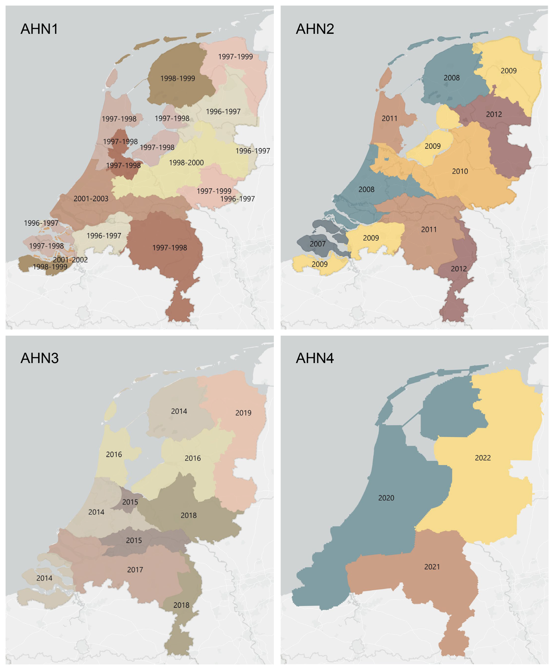
Figure 1 Data acquisition times for AHN1–AHN4. Different colours indicate the different years of data collection for each dataset.

Table 1 Summary of raw point cloud characteristics collected by different AHN surveys (AHN1–AHN4). Some flight configurations are not available, for instance, the type of sensor, the flight height, flight speed, and the scan angle, especially for the AHN1 dataset. NAP: normal Amsterdam level.

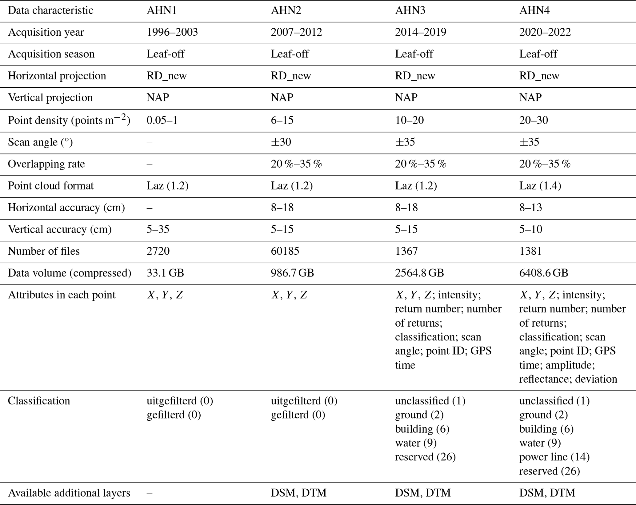
Benefitting from the advances in lidar sensors and related technologies, the third generation of the AHN programme (AHN3) provided not only a higher density of point clouds but also the storage of more information for each point, such as point classification code, intensity values, and number of returns (Table 1). Even though both AHN2 and AHN3 were collected within a 6-year cycle (2007–2012 for AHN2 and 2014–2019 for AHN3), the actual time difference between AHN2 and AHN3 varies between 4–10 years depending on the area of interest (Fig. 1). For the latest completed AHN survey (i.e. AHN4), the sampling was conducted between 2020 and 2022 (3-year cycle), making the country-wide dataset more quickly available for the whole of the Netherlands. All four AHN datasets were provided in LAZ format (i.e. version 1.2 for AHN1–AHN3 and version 1.4 for AHN4) under the local Dutch coordinate system “RD_new” (EPSG: 28992, NAP: 5709). The datasets from AHN1 to AHN4 show an increase in data volume and improved classification, as well as the storage of additional attributes for each point (Table 1). An ongoing fifth ALS survey (AHN5) started in 2023 (the first part of the data is available; see https://www.ahn.nl/heel-westelijk-nederland-gereed, last access: 24 July 2025), and the data acquisition will be completed in 2025.

2.3 Processing workflow

We employed the high-throughput workflow “Laserfarm” (https://laserfarm.readthedocs.io/en/latest/, last access: 24 July 2025) to process the multi-temporal AHN datasets. Laserfarm is an open-source workflow designed for processing large amounts of lidar point cloud data into geospatial data products of ecosystem structure (Kissling et al., 2022). It builds on the feature extraction module of the open-source “Laserchicken” software to compute lidar metrics (Meijer et al., 2020). The Laserfarm workflow consists of four main modules: (1) re-tiling, where the original LAZ files (covering 5 km × 6.5 km per tile) are re-tiled into 1 km × 1 km LAZ files for an efficient, scalable, and distributed processing; (2) normalization, where a DTM is constructed using the lowest point within a given grid cell (1 m  × 1 m), with every point in the cell then being assigned a normalized height with respect to the derived DTM height so that the influence of terrain is removed from subsequent processing (note that outliers with z values higher than 10 000 m were removed from further processing); (3) feature extraction, where user-defined features (e.g. lidar metrics such as the 95th percentile of vegetation height and the skewness of vegetation height) are calculated at 10 m resolution using points within an infinite square cell (i.e. a 3D square column with a base area of 10 m × 10 m and an infinite z value) (Meijer et al., 2020); and (4) rasterization, where the extracted feature files (.PLY files) are merged and exported as single-band GeoTIFF raster files. Note that, in all four AHN datasets, vegetation points are not classified separately based on the ASPRS standard. Instead, they are assigned a classification value of 0 (“uitgefilterd”) in AHN1 and AHN2 and a value of 1 (“unclassified”) in AHN3 and AHN4. These classification values were used as the vegetation class during the feature extraction. We chose the Laserfarm workflow to process the four country-wide AHN datasets because (1) it enables the efficient, scalable, and distributed processing of multi-terabyte lidar point clouds at a national scale; (2) it is a free and open-source tool implemented in Python and available in the form of Jupyter Notebooks; and (3) it allows for the automated generation of consistent and reproducible geospatial data products of ecosystems structure from different ALS data.

Due to the different characteristics of each AHN dataset (Table 1), several pre-processing steps were implemented before executing the main modules of the Laserfarm workflow (Fig. 2). In particular, for the AHN1 and AHN2 datasets, the step of “reclassification” was carried out before re-tiling as both datasets only have “gefilterd” (ground) and “uitgefilterd” (non-ground) files provided, and the raw classification value was set to 0 (never classified) for all points. We therefore reassigned a classification value of 2 to the ground points (“gefilterd”) and a classification value of 0 to the non-ground points (“uitgefilterd”). These classification values were later used for filtering the points during feature extraction. Note that there is no publicly available information on the methods and/or algorithms used in the pre-classification, and it is therefore difficult to assess the accuracy of the pre-classification of the AHN datasets. However, a preliminary assessment of the terrain-filtering process in the Dutch coastal dunes did not reveal a strong impact of the ground point pre-classification of AHN datasets on vegetation change detection (Appendix C). For the AHN4 dataset, the volume of a single original LAZ file varies from 0.3 MB to 16.5 GB, with an average size of 4.6 GB per file (Table 2). Since handling such volumes is challenging for many computing infrastructures (due to their CPUs and random-access memory or RAM), we applied a “splitting” step before the re-tiling (Fig. 2), with a maximum data volume of ∼500 MB being used for splitting the original tiles into smaller ones.

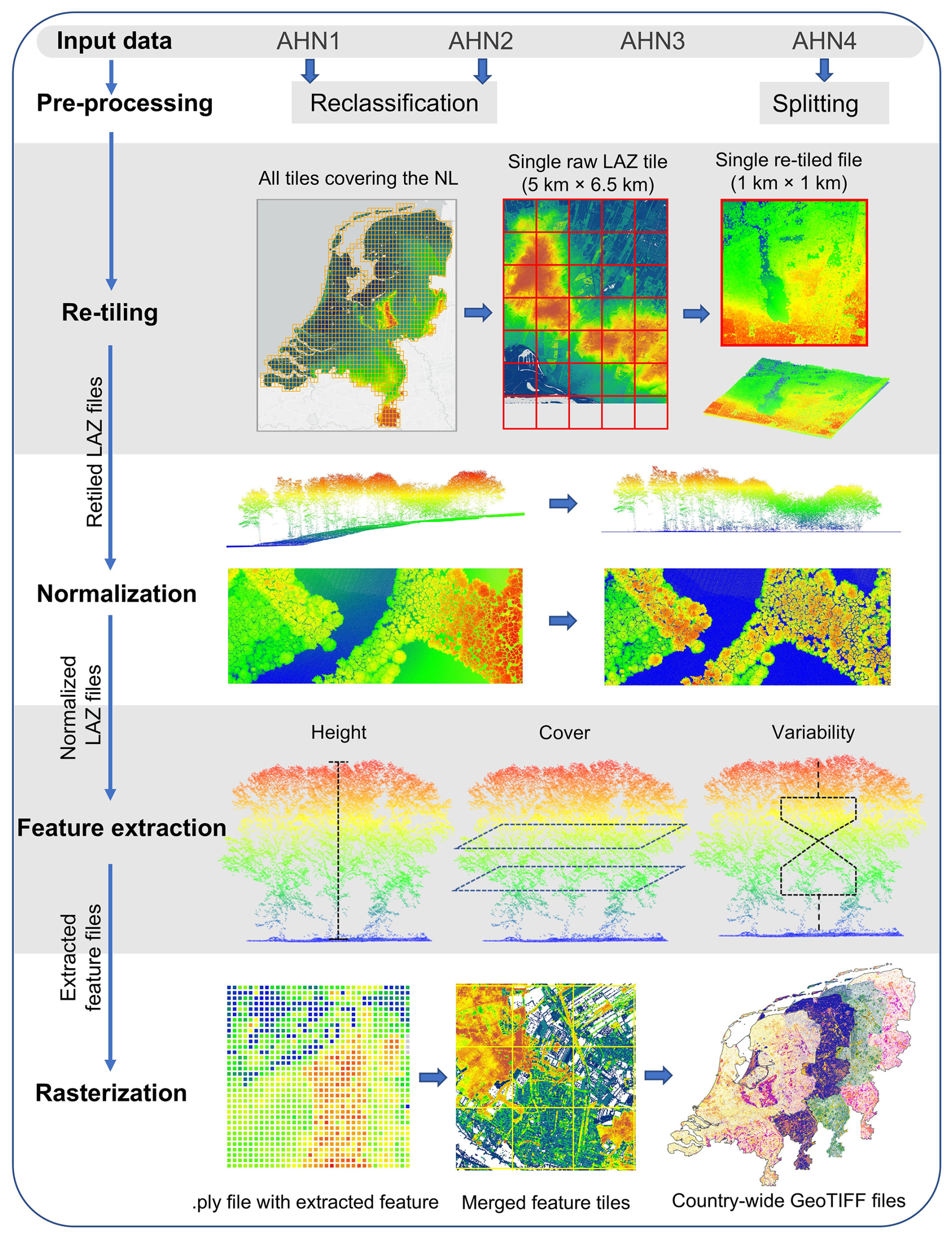
Figure 2 Overview of the processing workflow employed for four country-wide AHN datasets of the Netherlands (AHN1–AHN4). The pre-processing step “reclassification” was only conducted for the AHN1 and AHN2 datasets, where ground points were reassigned a classification value of 2. The splitting step was added to split the large LAZ files from AHN4 into smaller ones before re-tiling. Re-tiling, normalization, feature extraction, and rasterization are the four main modules of the Laserfarm workflow, which has been applied for all four AHN datasets to generate country-wide lidar-derived vegetation metrics. The input data were raw LAZ files with different point densities, and the output data were 25 single-band GeoTIFF raster layers at 10 m resolution for each AHN dataset.

2.4 IT infrastructure and computational cost

All four AHN datasets were processed on the IT infrastructure services provide by SURF, the Dutch national facility for information and communication technology (https://www.surf.nl/, last access: 24 July 2025). Specifically, we used the dCache platform for data storage (https://www.surf.nl/en/services/dcache, last access: 24 July 2025) and the HPC (high-performance computing) Cloud (https://www.surf.nl/en/services/hpc-cloud, last access: 24 July 2025) or Spider platform (https://www.surf.nl/en/services/high-performance-data-processing, last access: 24 July 2025) for high-performance data processing. The data processing platforms have fast access to the data storage while enabling scalable and flexible processing of multi-terabyte datasets on distributed resources. We first downloaded the raw AHN1–AHN4 lidar point clouds from the PDOK web services (https://www.pdok.nl/introductie/-/article/actueel-hoogtebestand-nederland-ahn, last access: 24 July 2025) to the dCache data storage using a customized Python script (https://github.com/ShiYifang/AHN/tree/main/AHN_downloading, last access: 24 July 2025). We then ran the Laserfarm workflow for processing the AHN1–AHN3 datasets on the HPC Cloud, where we set up a cluster of 11 virtual machines (VMs), with each VM having two cores, 32 GB or 64 GB RAM, and 256 GB local hard disc drive (HDD). Due to migration of the computing resources by SURF (from HPC Cloud to Spider), we processed the AHN4 dataset with the Laserfarm workflow on Spider, where a number of flexible and customizable workers with assigned CPU cores were defined based on the computing requirement for each workflow step. We used 2–10 workers, each with 2–4 cores and 16–32 GB RAM, for splitting, re-tiling, normalization, and feature extraction and 2 workers, each with 12 cores and 94 GB RAM, for the rasterization step. All input data (i.e. raw LAZ files), intermediate results (e.g. re-tiled LAZ files, normalized LAZ files, featured PLY tiles), and final outputs (i.e. GeoTIFF raster layers) were automatically stored (and/or retrieved for the next step) in the dCache data storage.

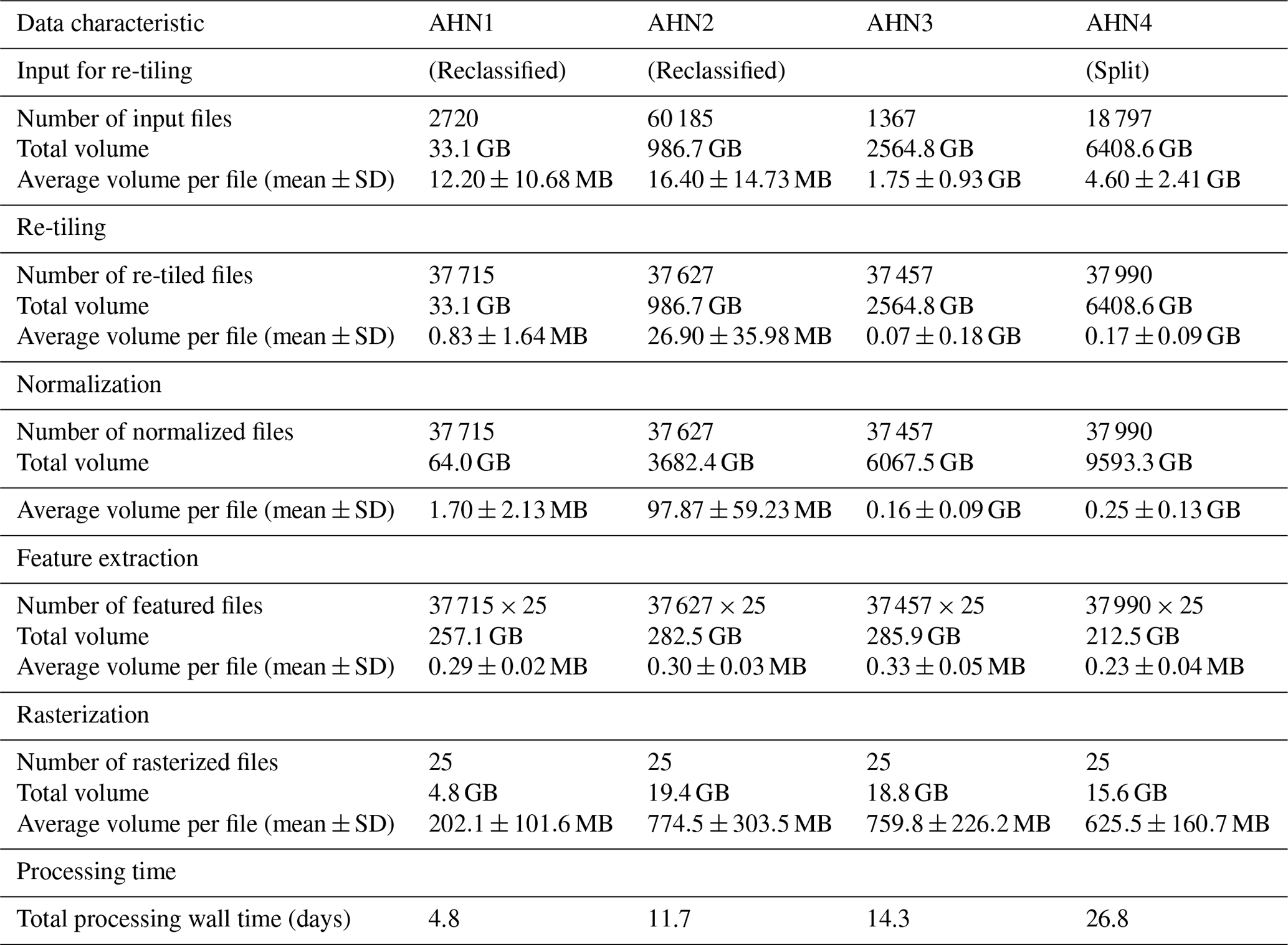
The computing time for each AHN dataset varies based on the input data volume, the required processing steps (Table 2), and the settings of the employed infrastructure. The increase in data volume from AHN1 to AHN4 resulted in a strong increase in the processing time (Table 2). In total, it required 57.6 d (wall time) to process the multi-temporal AHN datasets (AHN1–AHN4). AHN1 (data volume of 33.1 GB) only took a wall time of 4.8 d to complete, whereas AHN4 (data volume of 6408.6 GB) took a total wall time of 26.8 d. It is worth noting that the actual computing time of the process might be longer than the wall-time estimates, e.g. due to processing errors, worker failures, and system maintenance.

Table 2 Overview of the number of input files, the total volume and the average volume per file for each processing step, and the total processing wall time for each AHN dataset. Note that the total wall time was estimated based on different infrastructure settings for processing the AHN1–AHN3 (HPC Cloud) and AHN4 (Spider) datasets.

3 Data product description

3.1 Overview of data products

The generated data products from each AHN campaign cover the whole of the Netherlands, ranging from 50.77 to 53.36° N and from 3.57 to 7.11° E. The data products are provided as 10 m resolution GeoTIFF raster files (25 single-band raster layers for each AHN dataset) in the local Dutch coordinate system RD_new (EPSG: 28992, NAP: 5709). The total volume of the four sets of 25 lidar metrics is approximately 59.2 GB, and the total volume of additional masks and auxiliary data is 12.3 GB. The pixel value is stored in 32-bit floating-point precision. The data products are freely accessible via a permanent Zenodo repository (see Sect. 6).

3.2 Lidar-derived vegetation metrics

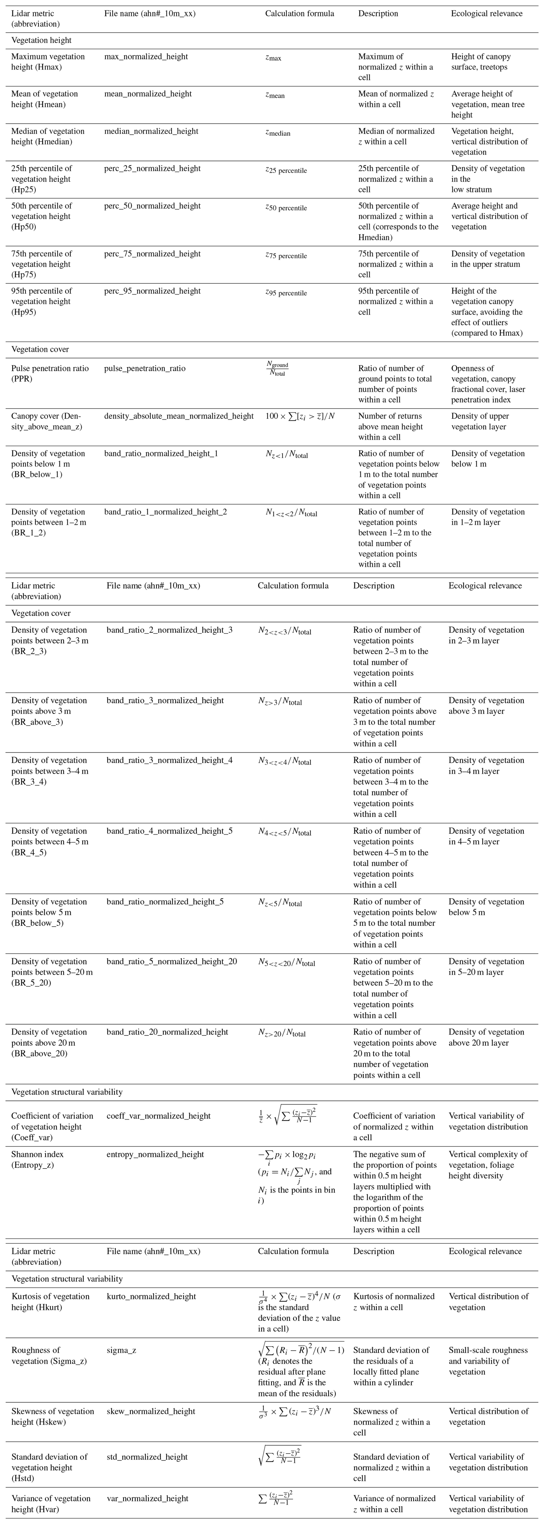
In total, 25 lidar-derived vegetation metrics were generated from each AHN dataset, representing vegetation height, vegetation cover, and vegetation structure variability (Table 3). For vegetation height, we generated seven lidar metrics (i.e. maximum; mean; median; and 25th, 50th, 75th, and 95th percentile of vegetation height) representing the height of the vegetation at the canopy surface and for low, middle, and upper vegetation strata (Fig. 3a). For vegetation cover, we derived 11 lidar metrics consisting of 1 metric describing the openness of vegetation (i.e. pulse penetration ratio), 1 metric describing the density of the upper vegetation layer (i.e. canopy cover), and 9 metrics quantifying vegetation density at different height layers (i.e. below 1 m, 1–2 m, 2–3 m, 3–4 m, 4–5 m, 5–20 m, above 3 m, below 5 m, and above 20 m) (Fig. 3b). The height layers reflect the most relevant height strata to capture the vegetation distribution of major growth forms (e.g. grass, reed, shrubs, and trees) (Morsdorf et al., 2010; Miura and Jones, 2010). Special attention was given to representing low-vegetation strata (1–5 m) as they are essential for low-stature terrestrial ecosystems such as grasslands, shrublands, or agricultural areas when monitoring animal habitats and species distributions (Koma et al., 2021a; Bakx et al., 2019). Note that the pulse penetration ratio is the only lidar metric (among the 25 metrics) that used ground points for the calculation. All of the other 24 metrics are only calculated with vegetation points (i.e. “unclassified” in AHN). For vegetation structural variability, we derived seven lidar metrics representing the vertical variability of the vegetation distribution within a cell (Fig. 3c), including the coefficient of variation, Shannon index, kurtosis, skewness, standard deviation, variance, and roughness (sigma) of vegetation height. The detailed description of how these metrics are calculated and of their ecological relevance can be found in Table 3.

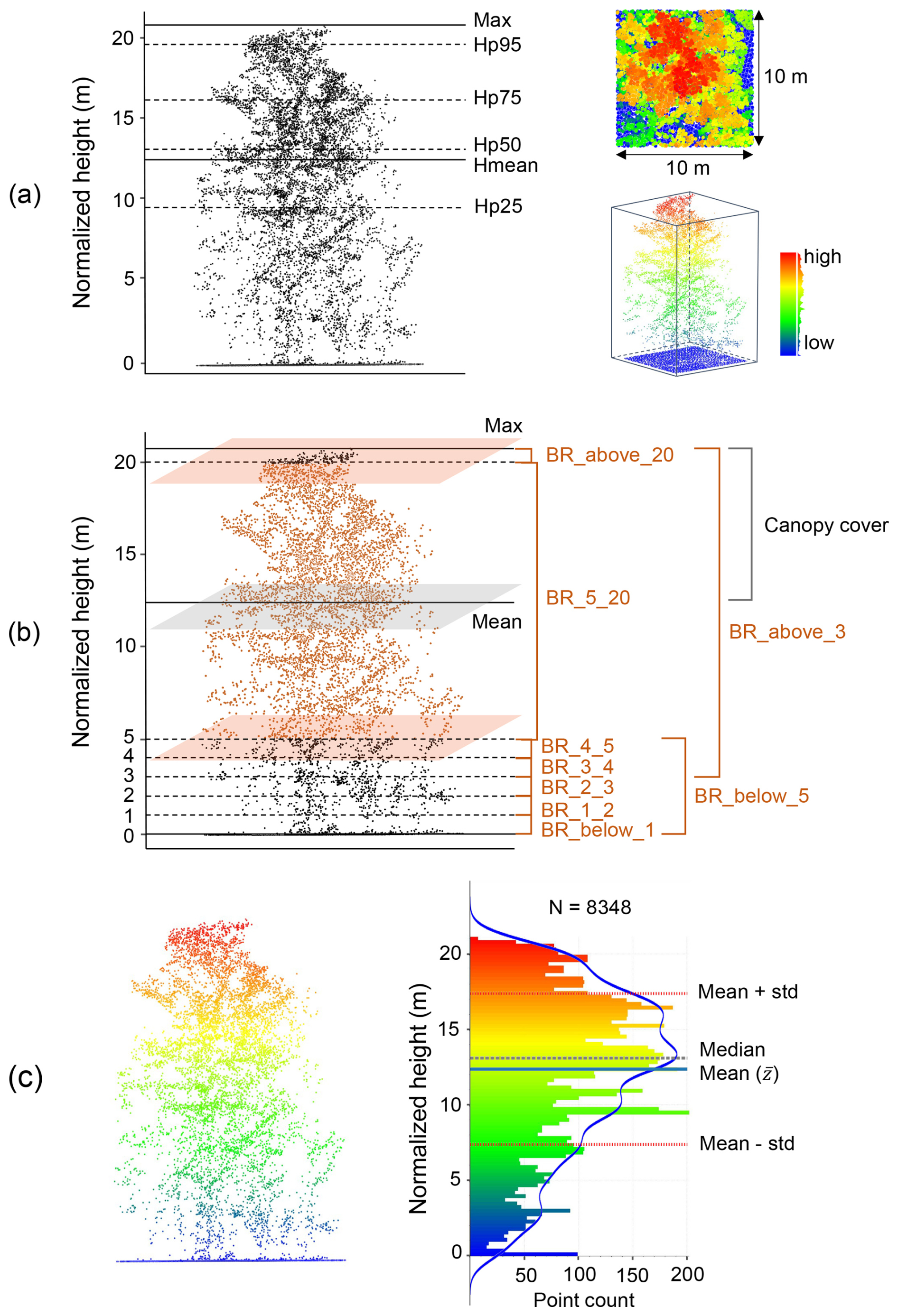
Figure 3 Examples of lidar metric generation in a 10 m × 10 m grid cell (the number of all points: N=8348). (a) Metrics of vegetation height (mean, max, and percentiles of normalized height). (b) Vegetation cover metrics representing vegetation density within specific height layers (e.g. “BR_4_5” indicates the vegetation density between 4–5 m; feature name: “band_ratio_4_normalized_height_5”). (c) Metrics of vegetation structural variability (e.g. standard deviation and variance of vegetation height are calculated based on mean height $\stackrel{\mathrm{‾}}{z}$; kurtosis and skewness of vegetation height are calculated based on the standard deviation and mean height within a cell) (see detailed calculation formula in Table 3). The blue line in (c) represents a kernel density estimate (KDE) showing the shape of the point distribution. See abbreviations and calculation formulae of all metrics in Table 3.

Table 3 The 25 lidar-derived vegetation metrics capturing ecosystem structure in three key dimensions (vegetation height, vegetation cover, and vegetation structural variability), together with their file names in the data products, the formulae for calculation, their descriptions, and examples of their ecological relevance. Each lidar metric is provided as a single-band GeoTIFF raster layer at 10 m resolution, with the file name “ahn#_10m_xx”, where # is the number of the AHN campaign (“1–4”), and xx is the name of the lidar metrics. For instance, “ahn4_10m_perc_95_normalized_height” represents the 95th percentile of vegetation height derived from the AHN4 dataset. For the calculation formulae, N is the total number of normalized vegetation points within a cell, z_i represents all normalized z values in a cell, and $\stackrel{\mathrm{‾}}{z}$ is the mean normalized z value in a cell.

3.3 Auxiliary data

Since the point density of AHN datasets changes across space and time, we also provide a raster layer of point density (using all point classes) for each AHN dataset (four in total) (Fig. 4). AHN1 has a much lower point density (average of less than 0.5 points m⁻²) throughout the whole country compared to the other AHN datasets due to sensor limitations back in 1996. AHN2 and AHN3 have a similar point density (on average, 10–20 points m⁻²), while AHN4 has the highest point density (25–30 points m⁻²). Especially for the AHN2–AHN4 datasets, distinct patterns (e.g. patches, lines, edges) can be observed in different parts of the Netherlands. These are partially due to the influence of the water surface (yellow areas in AHN2, AHN3, and AHN4; see Fig. 4) but are also related to flight lines and operational configurations (e.g. flying altitude and flight speed) during the campaign.

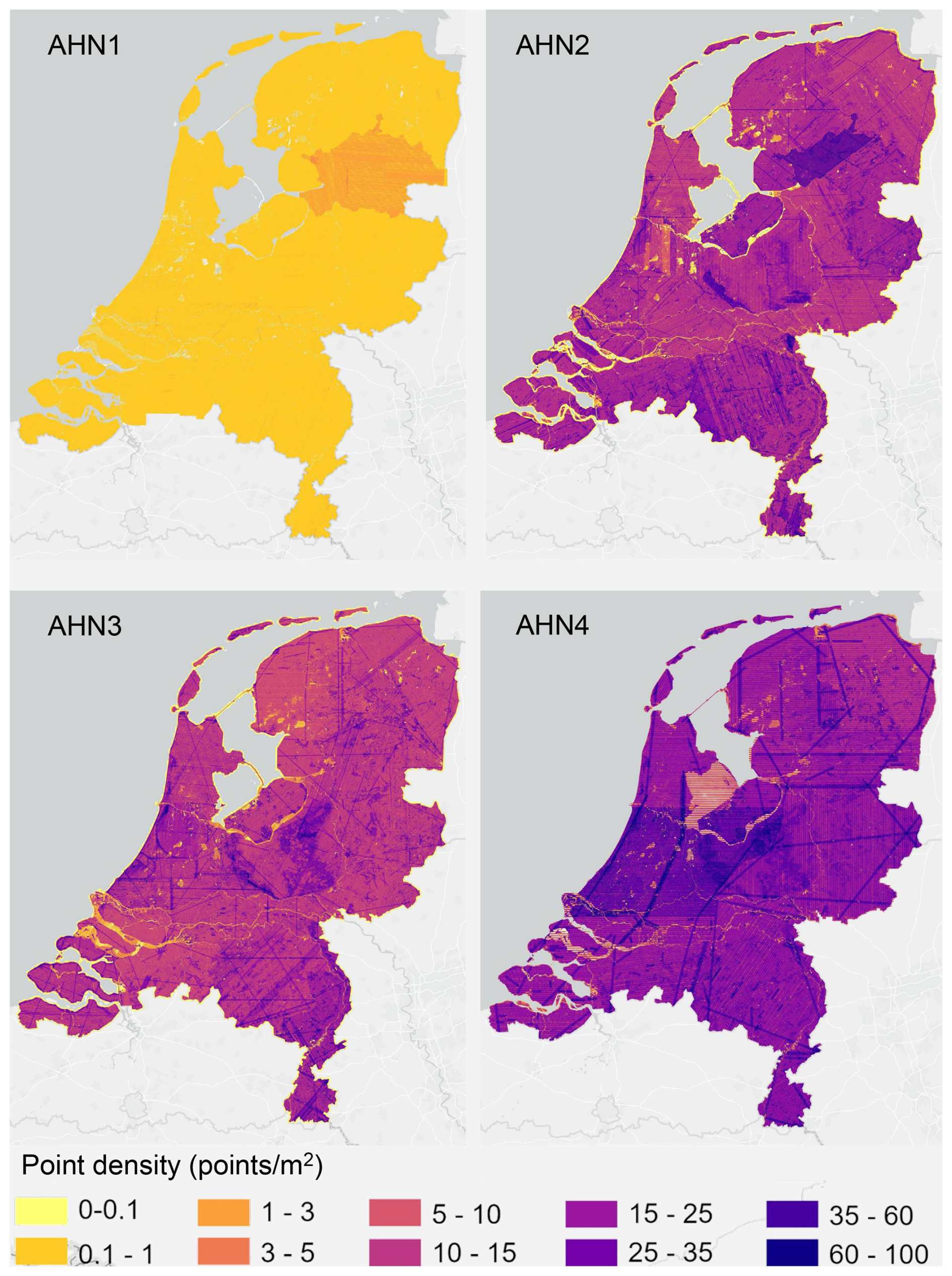
Figure 4 Point density of AHN1–AHN4 ALS campaigns across the Netherlands. The total number of points was used for calculating the density of points at 10 m spatial resolution. The four point density layers are made available in the data repository as auxiliary data together with the derived lidar metrics (see Sect. 6).

In addition to point density (i.e. density of all return points), we also provide raster layers of pulse density (i.e. density of first return points) for the AHN3 and AHN4 datasets. Pulse density is less instrument dependent than point density and more directly reflects the scan quality and condition. Since there is no pulse information available from the AHN1 and AHN2 datasets, we only provide pulse density layers for AHN3 and AHN4. The two pulse density layers are made available in the data repository as auxiliary data together with the derived lidar metrics (see Sect. 6).

Although AHN campaigns have been conducted during the leaf-off season, the actual date/month during which an area is scanned can vary from December (late winter) to April (early spring), making it difficult to distinguish actual vegetation change (over the years) from leaf phenology. We therefore provide the flight line timestamps as raster layers with a 10 m resolution for comparing the dates of data acquisition across the datasets and generated properties. For AHN3 and AHN4, we first downloaded the flight line vector layers from https://www.ahn.nl/dataroom (last access: 24 July 2025) and then generated a buffer zone around the flight lines using the function “Buffer” in ArcGIS Pro (version 3.3.0), with the setting of a distance (on both sides of each flight line) of 300 m for AHN3 and of 700 m for AHN4. The neighbouring buffer zones were then dissolved if they had the same flight time. The specific distance value of the buffer zone was derived from the distance between two flight lines in each AHN survey. We then rasterized the generated buffer zone polygons into raster layers at 10 m resolution using the “Polygon to Raster” function in ArcGIS Pro. In areas where multiple flight lines are overlapping, we assigned the latest flight date to the raster pixel to be in line with the flight year maps provided by the AHN programme (see Fig. 1). Users should take the surrounding pixel values into account when investigating overlapping areas. The generated timestamp layers for AHN3 and AHN4 are made available in the same data repository as the data products (see Sect. 6).

Although the AHN provides DTM and DSM layers at 0.5 and 5 m resolution for AHN2–AHN4, these do not come at the same spatial resolution as the generated lidar-derived vegetation metrics. To facilitate users in comparing DTMs and DSMs with the generated lidar metrics, we generated DTM and DSM layers at 10 m resolution for each AHN datasets (except AHN1). The generated DTM and DSM layers were derived by resampling DTM and DSM tiles provided by the AHN to a 10 m resolution using an unweighted average method. The Jupyter Notebook used for this step is made available in GitHub (see Sect. 7).

3.4 Limitations and usage notes

3.4.1 Classification-related errors and masks

In the pre-classification of the raw AHN point clouds, there is no “vegetation” class provided based on the ASPRS standard (i.e. class 3: low vegetation; class 4: medium vegetation; or class 5: high vegetation). Instead, the vegetation points in the raw AHN1 and AHN2 datasets are included in the non-ground class (“uitgefilterd”, classification value of 0), whereas they belong to the “unclassified” class (classification value of 1) in the AHN3 and AHN4 datasets (Table 1). This can introduce errors and biases when using the “uitgefilterd” or “unclassified” class for calculating ecosystem structure properties because points belonging to human infrastructures can still be included in these classes. In particular, buildings and bridges are included (together with objects other than ground) in the “uitgefilterd” class in the AHN1 and AHN2 datasets, while they are classified separately (buildings in class 6: “buildings”, and bridges in class 26: “reserved”) in the AHN3 and AHN4 datasets, eliminating the errors caused by buildings and bridges in the final data products of the AHN3 and AHN4. Power lines are not separated from the “uitgefilterd” class in the AHN1 and AHN2 datasets and are included in the “unclassified” class in the AHN3 dataset, but, in the AHN4 dataset, they are separately classified as class 14: “power line”. Yet, other human objects and infrastructures (e.g. cars, fences, and transmission towers) are not separated in any of the four AHN datasets and are thus included in the non-ground class (“uitgefilterd”) of the AHN1 and AHN2 datasets and in the “unclassified” class in the AHN3 and AHN4 datasets, introducing some errors and biases into the final data products. There are also points appearing on water surfaces (e.g. reflected by boats and birds) which are included in the “uitgefilterd” or “unclassified” class, causing inaccuracies in the final products. In a previous study (Kissling et al., 2023), the accuracy of the 25 lidar metrics generated from the AHN3 dataset was assessed, particularly in relation to the error caused by using the “unclassified” class for calculating ecosystem structure properties. The results showed that the overall accuracy of the generated lidar metrics was high (0.90±0.04, n=25 lidar metrics, tested for 100 randomly selected plots throughout the Netherlands, with 10 m × 10 m size per plot), ranging from 0.87 to 1. It is worth noting that the impact of those errors on the 25 lidar metrics varies; for instance, a stronger bias (i.e. the difference between the generated lidar metrics and the ground truth) can be observed in height metrics describing the top canopy layer (i.e. Hmax and Hp95) compared to in other height metrics or in metrics of vegetation cover in the low strata (i.e. BR_below_1 and BR_below_5) (Kissling et al., 2023).

To minimize the inaccuracies of the data products as caused by human infrastructures and water surfaces, we provide mask layers of water areas, roads, and buildings for both the AHN3 and AHN4 data products based on the Dutch cadastral data (TOP10NL) from 2018 (corresponding to AHN3) and 2021 (corresponding to AHN4) (https://www.kadaster.nl/zakelijk/producten/geo-informatie/topnl, last access: 24 July 2025). TOP10NL is part of the Basic Topography Registry (BRT), which provides the standard topographic base files for the whole of the Netherlands. Like the lidar metrics, the masks are calculated at 10 m resolution with the RD_new/EPSG 28992 projection coordinate system and provided as raster layers in GeoTIFF format. In the masks, water surfaces, buildings, and roads were merged into one class with an assigned pixel value of 1, and the rest were merged into one class with a pixel value of 0 (Fig. 5). Since the historical versions of TOP10NL data are not available for AHN1 (1996–2003) and AHN2 (2007–2012), we can only provide the masks for the AHN3 and AHN4 datasets (see Sect. 6 for data availability). However, despite the potential changes in buildings and roads over time, it is still possible to apply the generated masks to all four AHN data products, for instance, to minimize errors and to have comparable areas of interest. Note that water surfaces were already masked out from the pulse penetration ratio layers by removing 0 values that result from areas with waterbodies (i.e. falsely indicating dense vegetation). This was done by masking out water areas (from TOP10NL) from the pulse penetration ratio layers using the “Extract by Mask” function in ArcGIS Pro. Areas with buildings and roads have the value of 1 in the pulse penetration ratio layers, which indicates total openness (no vegetation).

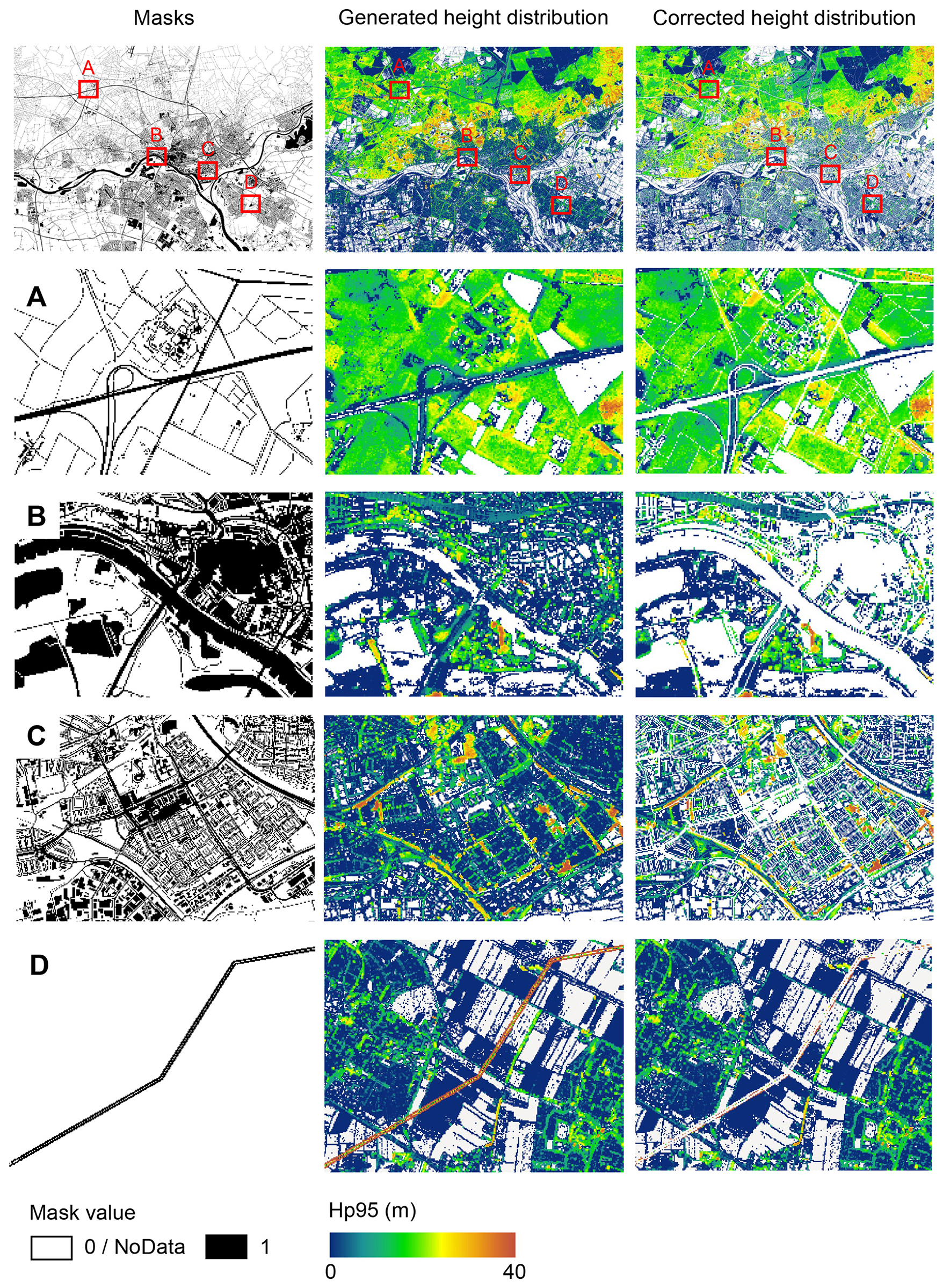
Figure 5 Examples of masking roads, water surfaces, and buildings as derived from the 2018 Dutch cadastral data (areas A, B, and C) and power lines generated from the AHN4 dataset (area D). Illustrated is the rasterized mask (first column), the generated vegetation height metric (i.e. Hp95) from AHN3 (second column), and the corrected vegetation height using the masks (third column). Four subareas show the inaccuracies in the originally generated vegetation height metric and the removal effect of using the mask for roads (area A), water (area B), buildings (area C), and power lines (area D). A mask value of 1 represents the pixels with roads, water surfaces, buildings, and power lines, while a value of 0 or the label “NoData” represents the rest. The masks and the lidar metrics are at 10×10 m resolution. The subareas A–D are located around Arnhem in the east of the Netherlands (51.9825248° N, 5.9102228° E). Hp95 denotes the 95th percentile of vegetation height.

Since power lines are not classified separately for the AHN1–AHN3 datasets and thus are included in the vegetation metric calculation, this may cause abnormal values of vegetation structure, especially for vegetation height and vegetation cover above 20 m (Shi and Kissling, 2023). However, in AHN4, the points belonging to power lines are classified separately (Table 1), which provides a way to minimize errors caused by power lines in the data products generated using AHN1–AHN3. We therefore extracted all power line points from the AHN4 raw point cloud and generated a mask (at 10 m resolution) where pixels containing power lines are assigned a value of 1 and the rest are labelled with “NoData” (Fig. 5). Since the transmission towers are not classified separately in all four AHN datasets, the mask covers only the power lines and not the transmission towers. Users can apply the power line mask generated from AHN4 to the data products from AHN1–AHN3 and consequently improve the comparability of the lidar metrics across time. Note that the power line infrastructure may also change over time, and the classification of power lines using AHN4 may thus not fully represent the power line distributions in earlier time periods.

3.4.2 Strip issues

Several strip patterns occur in the data products from AHN2 (Fig. 6). These strip issues specifically affect the pulse penetration ratio layer (representing vegetation openness), where both ground points (ground class) and vegetation points (“unclassified” class) were used for the metric calculation. A possible reason for this could be that the scan angle of the laser scanner used for point cloud acquisition was rather wide, and so the scanner received more laser pulses from the areas located at the edges of the flight lines. Those overlapping areas (edges of the flight lines) often have a doubled point density, which also contributes to the strip patterns in the calculation of the lidar metrics using ground points (e.g. pulse penetration ratio). This issue mostly occurs in an area in the centre of the Netherlands (Fig. 6). Some vegetation density metrics (e.g. BR_below_1, BR_below_5) also seem to be influenced by this strip issue.

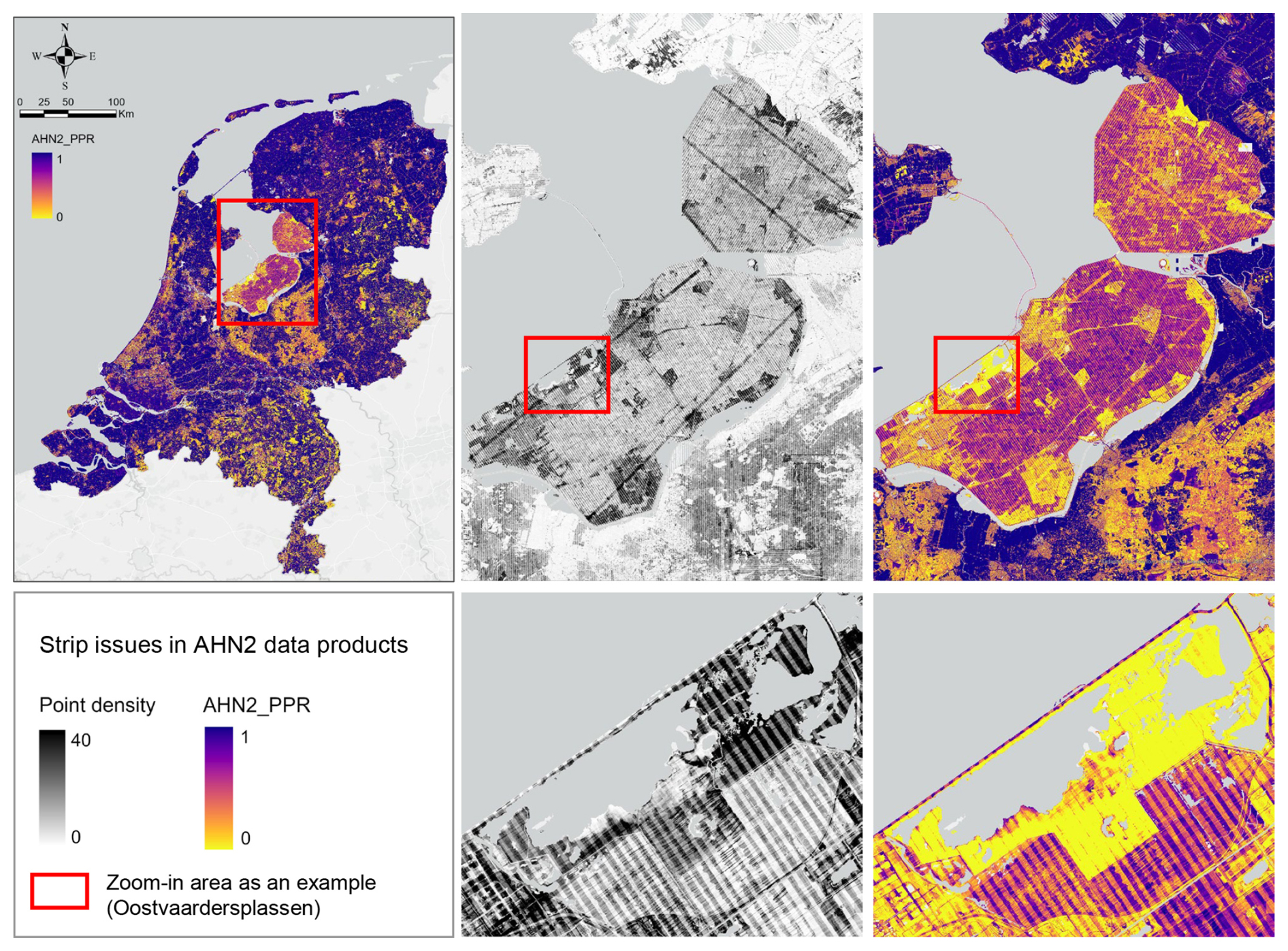
Figure 6 Strip issues in the AHN2 dataset. The point density (black and white, including all points) and the pulse penetration ratio (colour, representing vegetation openness) show similar strip patterns.

3.4.3 Abnormal values

A few pixels with abnormal values still exist in the final products. For instance, several pixels in the Hp95 layer have a value higher than 100 m, which cannot represent the upper canopy of vegetation since the tallest tree in the Netherlands (a Douglas fir, Pseudotsuga menziesii, i.e. a tall and fast-growing conifer native to western North America, which was planted between 1860 and 1870 in Apeldoorn, the Netherlands) has been measured to be ∼50 m tall. More generally, most measurements of the tallest trees in the Netherlands range between 20–45 m. Hence, abnormal values of vegetation height (e.g. >50 m) most likely reflect the occurrence of human infrastructures that are not included in the AHN1 and AHN2 “uitgefilterd” class or that are not sufficiently captured in the AHN3 and AHN4 “building” and “reserved” classes, e.g. aerial and radio masts (up to 350 m tall), tall industrial and meteorological towers and chimneys (50–200 m), cranes (50–130 m), elements of bridges (e.g. pylons and steel cables up to 140 m tall), wind turbines (up to 260 m), and power lines (up to 80 m). Flying objects, such as birds and planes, can also be captured in the datasets, resulting in abnormal height values in the data products. We recommend filtering out those abnormal values before using the data products for further analysis, e.g. by removing grid cells with Hp95 > 50 m, Hp95 > 40 m, or Hp95  > 30 m.

Although the Netherlands has a rather flat terrain, it is worth noting that the normalization method implemented in the Laserfarm workflow may introduce inaccuracies into normalized vegetation height values, especially if steep terrain occurs within a grid cell (Kissling et al., 2022). When applying the same workflow to other countries or regions, abnormal values may occur in areas with drastic topographic changes (e.g. cliffs, mountainous area). Users may consider using a different normalization method, for instance, normalizing non-ground points by subtracting the derived DTM from all points or by interpolating the elevation of non-ground points using the exact position of ground points beneath (Roussel et al., 2020). Some studies also suggest using raw point clouds (e.g. the non-normalized DSM) to preserve the geometry of treetops or plant area index profiles in high-slope areas (Khosravipour et al., 2015; Liu et al., 2017).

Since we only used the points from the “unclassified” class of the AHN datasets for calculating vegetation metrics (except for the pulse penetration ratio, for which all points were used), grid cells with no vegetation points resulted in NA values. Those areas are often bare ground, buildings, or waterbodies, which should be excluded from vegetation structure assessments. We therefore generated an NA value mask for each AHN dataset (AHN1–AHN4), which can be used for masking areas that potentially have no vegetation (see Sect. 6). Those NA value masks can also be combined and used for vegetation change detection across multi-temporal AHN data products. Note that NA values can also result in areas where very low vegetation is misclassified as ground points, given that the vertical accuracy of the z values in AHN products is typically 5–15 cm (Table 1). Hence, “no-vegetation areas” as derived from the NA value masks can differ from the real land cover.

3.4.4 Sensitivity analysis

We conducted a sensitivity analysis to gain a better understanding of the robustness of the lidar metrics in relation to the varying pulse densities of the different AHN datasets. We focused on pulse density (i.e. density of the first return points) instead of point density (i.e. density of all return points) as pulse density is less dependent on instrument-specific multiple-return detection capabilities. This makes it more directly related to the scanning parameters (e.g. pulse rate, scanning geometry) and conditions (e.g. flight speed, altitude), reflecting a clearer measure of scan quality. For the four completed AHN surveys, only AHN3 and AHN4 provide pulse information (e.g. “return number”, “number of returns”) in the point cloud, whereas AHN1 and AHN2 do not provide such information. For the latter two, we therefore approximated the pulse information by assuming a pulse density of one-quarter and one-half of AHN3. Since varying pulse density may have different impacts on lidar metrics from structurally different habitat types, we performed the sensitivity analysis for five main habitat types (i.e. dunes, marshes, grasslands, shrublands, and woodlands) within Natura 2000 sites in the Netherlands. For each habitat type, 100 sample plots (10 m × 10 m, 500 plots in total) were randomly selected, where Hp95 is not NA (assuming that vegetation occurring in the plots) (see details of plot selection in Appendix A). For each sample plot, the pulse density of AHN4 was systematically down-sampled to the same pulse density as AHN3 and then to one-half of the pulse density of AHN3 (assuming comparability with AHN2) and then, lastly, to one-quarter of the pulse density of AHN3 (assuming comparability with AHN1). For systematic down-sampling, we used the same methodology as described in Appendix B of Kissling et al. (2024a); i.e. the first return points were first sorted according to their GPS acquisition time (from earliest to latest) and then were down-sampled to the different densities. For instance, for woodlands, we down-sampled the pulse density from 25 pulses m⁻² (AHN4) to 14, 7, and 4 pulses m⁻². We then compared the 25 lidar metrics generated from the original AHN4 point cloud to those from the down-sampled point clouds for each habitat type. Our analysis revealed that almost all lidar-derived vegetation metrics in all habitats are robust in relation to varying pulse densities at 10 m resolution, even when calculated with strongly down-sampled pulse densities of ≤4 pulses m⁻² (see Figs. B1–B5 in the Appendix). The exceptions were canopy cover (Density_above_mean_z) and Shannon index (Entropy_z), which decrease markedly with lower pulse densities in all habitat types, and the coefficient of variation of vegetation height (Coeff_var) in grasslands and shrublands (see Figs. B3 and B4). Some metrics in grasslands also showed larger variability with down-sampled pulse densities.

Given the vertical accuracy of AHN2–AHN4 (i.e. 5–15 cm), classification-related errors, and the potential influence of data acquisition time, we suggest that small vegetation changes (e.g. less than 0.5–1 m) should be interpreted with caution. These can be influenced by vertical height uncertainties, low vegetation points being wrongly classified as ground points, or differences in leaf phenology due to varying data acquisition times rather than representing real vegetation changes. When comparing vegetation changes between the AHN3 and AHN4 metrics, users can make use of the flight time raster layers to take vegetation phenology differences into account. Based on our sensitivity analysis, we also suggest that users should be aware that some lidar metrics from open and heterogeneous habitats such as grasslands and shrublands might be less robust in relation to varying point and pulse densities compared to those from dunes, marshes, and woodlands.

4 Demonstration of ecological use cases

4.1 Monitoring forest structural change across time using multi-temporal ALS data

As a use case, we demonstrate here how the multi-temporal data products generated from the Dutch ALS surveys can capture forest structural change over the last 2 decades (2000–2023). We included the ongoing ALS campaign (AHN5) since the data were made available for the sample area (central location coordinates: 52.3250517° N, 5.7409230° E) at the time when the analysis was conducted. This provided a longer time series for detecting forest change. The sample area (in a forest area north of the national park De Hoge Veluwe) experienced a clear forest cut in 2011 (between the AHN2 and AHN3 surveys), with further forest loss and some regenerations captured by AHN4, while the latest AHN5 showed a forest regrowth in the middle–low-vegetation strata (<10 m) compared to AHN4 (Fig. 7). Based on the AHN point clouds, the average vegetation height changed from 20.9 m (SD: ±4.9 m) (AHN1) to 22.6 m (SD: ±8.0 m) (AHN2) and showed a drastic decrease from 18.0 m (SD: ±12.1 m) (AHN3) to 3.1 m (SD: ±4.9 m) (AHN4) and then a slight regrowth to 3.4 m (SD: ±2.6 m) (AHN5). The histograms derived directly from the AHN1–AHN5 point clouds show the distribution of points shifting from tall vegetation (above 20 m, AHN1–AHN3) to low vegetation (below 10 m, AHN4 and AHN5). Due to the very low point density of the AHN1 data, high-resolution information on vegetation structure in the year 2000 is lacking. However, the histogram from AHN1 implies a pattern of canopy height similar to that from AHN2 (Fig. 7). Google Earth images obtained for the closest available dates from each AHN survey also provide a good reference for the forest change events, except for the time of AHN1.

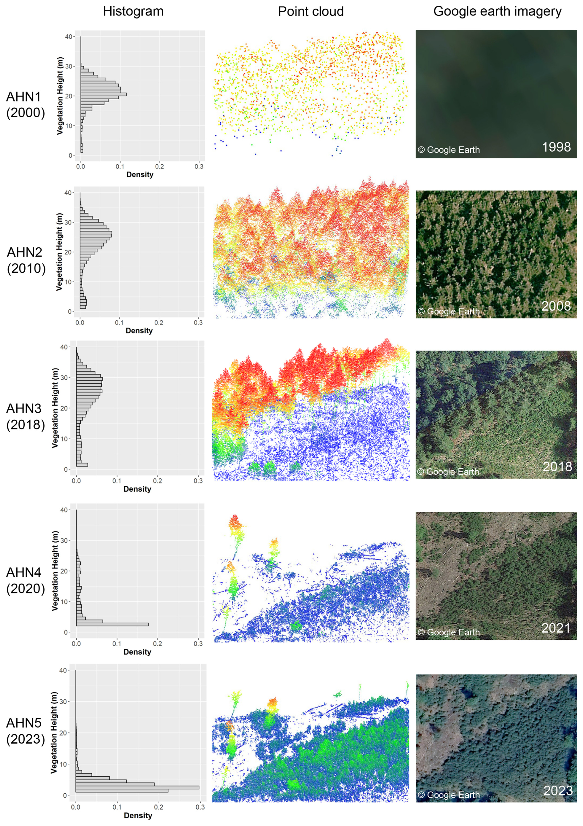
Figure 7 Forest structural change in a sample plot (100 m × 100 m) between 1998–2023 captured by the multi-temporal AHN datasets (AHN1–AHN5). The histograms were generated from each AHN point cloud, showing the distribution of the normalized vegetation height within the plot. The point clouds were coloured by height (blue indicates lower vegetation height, and red indicates higher vegetation height). AHN1 has a rather poor point density but shows a histogram of vegetation height that is similar to that of AHN2. The forest cut can be observed from the point clouds of AHN3 and AHN4 compared to AHN2, with forest regrowth occurring in AHN5. Google Earth images from the example area show the changes in the forest. Note that the dates of the Google Earth images do not correspond exactly to the dates of the airborne laser scanning surveys but rather to the closest dates available. Map data: © Google Earth.

Six selected lidar-derived vegetation metrics derived from AHN1–AHN5 at 10 m resolution effectively capture the changes in vegetation structure over time (Fig. 8). The 95th percentiles of vegetation height (Hp95) and mean vegetation height (Hmean) highlight reductions in forest canopy height due to cutting in 2011 (between AHN2 and AHN3) and in 2019 (between AHN3 and AHN4). The pulse penetration ratio (PPR) reveals shifts in vegetation openness, with openness peaking in AHN4, while the density of vegetation points at 2–3 m (BR_2_3) indicates regrowth in the understorey, particularly in AHN4 and AHN5 (after 2021). The Shannon index (entropy_z) reflects the vertical distribution of vegetation points (i.e. proportion of points within 0.5 m height layers), with AHN2 showing the highest value due to a more even point distribution of the canopy foliage before the canopy was cut. AHN3 shows the widest Shannon index range, capturing both high-canopy trees and new re-growth. The standard deviation (i.e. vertical variability) of vegetation height (Hstd) shows a pattern similar to that seen in Hp95.

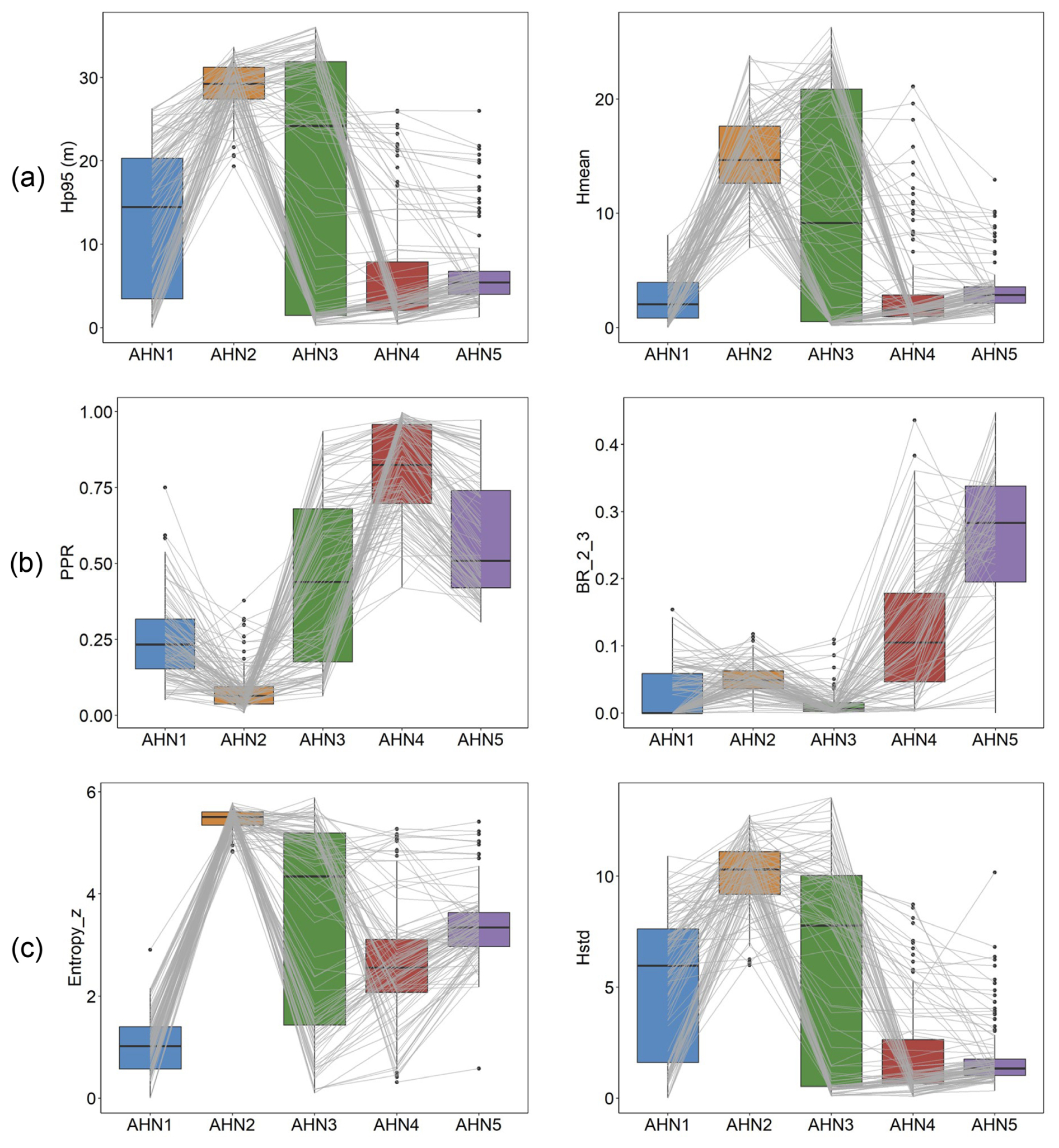
Figure 8 Boxplots of lidar metrics derived from multi-temporal AHN datasets capturing the changes in the vegetation structure in a 100 m × 100 m sample area (compare Fig. 7). (a) The 95th percentile of vegetation height (Hp95) and the mean vegetation height (Hmean) representing vegetation height. (b) The pulse penetration ratio (PPR) and the density of vegetation points between 2–3 m (BR_2_3) representing vegetation cover. (c) The Shannon index (Entropy_z) and the standard deviation of vegetation height (Hstd) representing vegetation structural variability. Boxes show the median and interquartile range, with whiskers extending to 1.5 times the interquartile range, and outliers are plotted as dots. Each grey line represents a single pixel (10 m × 10 m) value changing from AHN1 to AHN5, showing the influence of the events on vegetation within each pixel (e.g. forest cut and regrowth).

4.2 Comparison of vegetation structural differences within Natura 2000 sites

In a second use case, we analyse how vegetation structure varies spatially across different Natura 2000 habitat types in the Netherlands. Terrestrial habitats were categorized into five main classes – dunes, marshes, grasslands, shrublands, and woodlands – based on the dominant habitat type within each site (see details in Appendix A). For each habitat class, 100 random sample plots (10 m × 10 m, 500 plots in total) were selected, where Hp95 is not NA (assuming that vegetation occurs in the plots) (Fig. A1). We used the data products from AHN4 for the analysis as they are the latest complete products for the whole of the Netherlands. Four lidar metrics were compared: the 95th percentile of vegetation height (Hp95), vegetation point density at 1–2 m (BR_1_2) and 4–5 m (BR_4_5), and the coefficient of variation of vegetation height (Coeff_var). Structural differences among the five habitat types were assessed using the non-parametric Kruskal–Wallis test by ranks (Kruskal and Wallis, 1952), which compares two or more independent groups of equal or different sample sizes without assuming a normal distribution of the residuals. Pairwise comparisons of the statistical significance were conducted among groups (i.e. habitat types) using the Wilcoxon rank sum test (Wilcoxon et al., 1970).

The strongest structural differences among the five habitat types were observed in canopy height (Hp95) and vegetation density in the lower strata (BR_1_2), followed by vegetation vertical variability (Coeff_var) and vegetation density in the middle strata (BR_4_5) (Fig. 9). The canopy height (i.e. Hp95) of both woodlands and shrublands was highest and showed a statistically significant difference compared to all other habitat types, whereas grasslands, marshes, and dunes did not differ in terms of canopy height (Fig. 9a). The latter three habitat types showed a median canopy height of ∼2.3 m, whereas this is around 9.9 and 17.6 m for shrublands and woodlands, respectively. Vegetation density in the low-vegetation stratum (between 1–2 m) also did not differ statistically between grasslands, marshes, and dunes (Fig. 9b). However, woodlands and shrublands, with their more shaded understorey and stronger light competition, had, proportionally, much less vegetation in the lower layer (between 1–2 m) than the three open habitat types (Fig. 9b). In the mid-layer (4–5 m), only the vegetation density of woodlands and marshes showed a statistically significant difference (Fig. 9c). The low mid-layer density in woodlands reflects the fact that understorey shrubs are proportionally underrepresented compared to the vegetation density of high-canopy trees, whereas shrubs and trees in marshes can be abundant but may generally have a lower canopy height than woodland trees, thus showing high vegetation density at 4–5 m. In terms of structural variability, grasslands and marshes have the highest median values of the coefficient of variation of vegetation height across the 100 plots, showing significant differences compared to woodlands, shrublands, and dunes (Fig. 9d). This probably reflects a high heterogeneity in vegetation structure in both grasslands and marshes, where a large variability of low vegetation (grasses, herbs) and high vegetation (shrubs, trees) can be present within the 10 m × 10 m plots. It is also the only metric among the four selected metrics where dunes showed statistically significant differences compared to grasslands and marshes.

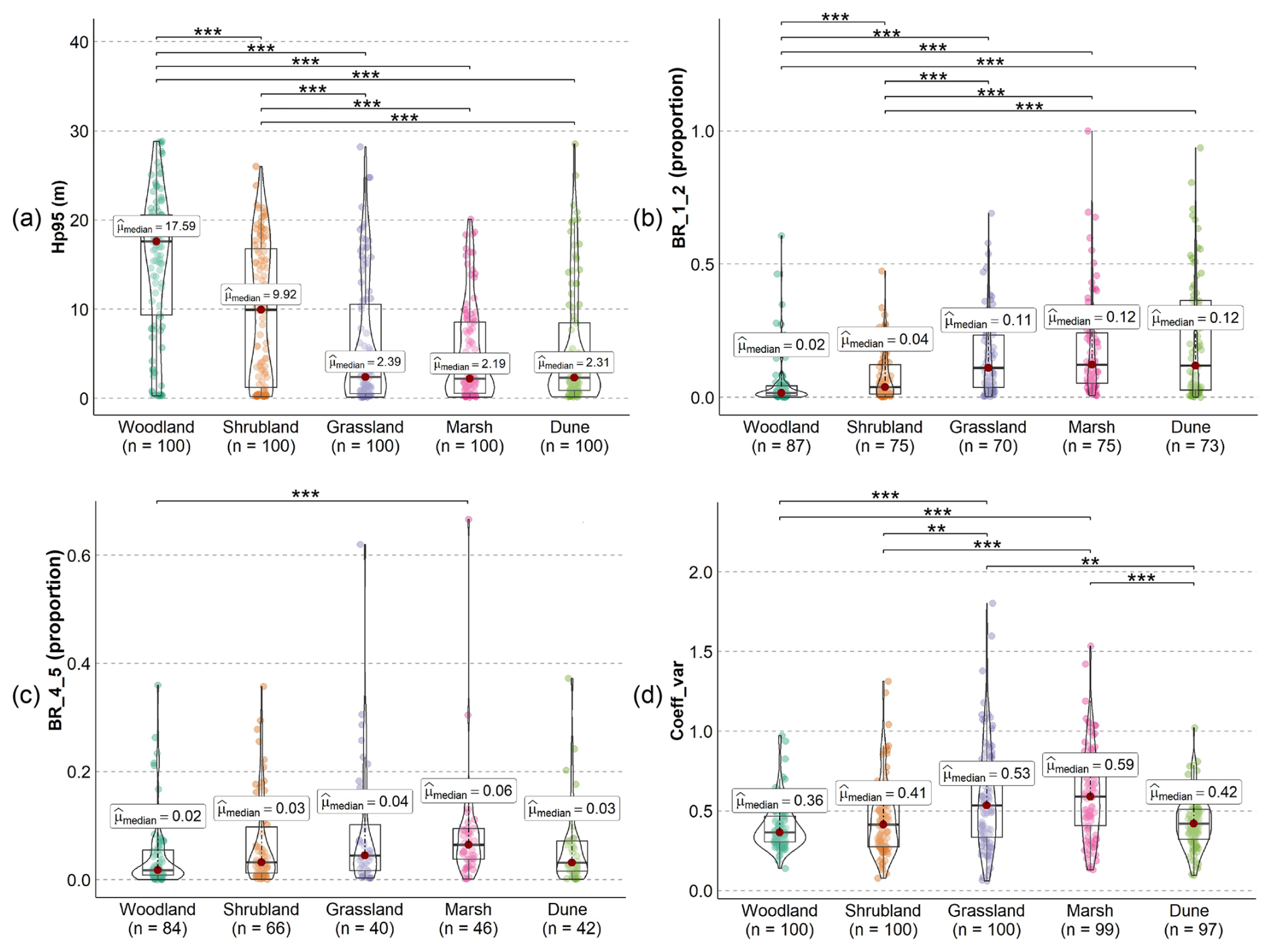
Figure 9 Comparison of ecosystem structure between five Natura 2000 habitat types using four different lidar metrics of vegetation structure. (a) Canopy height (the 95th percentile of vegetation height, Hp95), (b) vegetation density at 1–2 m (BR_1_2), (c) vegetation density at 4–5 m (BR_4_5), and (d) structural variability of vegetation height (coefficient of variation in vegetation height, Coeff_var). The bars above the violin plot indicate whether there is a statistical significance between two compared habitat types. The pairwise comparisons of the statistical significance were conducted using the Wilcoxon rank sum test after the non-parametric Kruskal–Wallis test by ranks. The significant level is marked as follows: ${}^{***}$ (p<0.001), ${}^{**}$ (p<0.01), and ^* (p<0.05). Red dots indicate the median value (${\widehat{\mathit{\mu }}}_{\mathrm{median}}$) of the lidar metrics measured for each habitat type. Note that not all sampled plots have vegetation points (from the “unclassified” class) between 1–2 m and between 4–5 m; therefore, the total number of sample plots for the BR_1_2 and BR_4_5 analysis was <100 for each habitat type (after removing the NA value). The NA value also occurs for Coeff_var when there is only one point (from the “unclassified” class) in the sampled plot (see metric calculation in Table 3).

5 Discussion

We present a set of multi-temporal high-resolution data products of ecosystem structure derived from country-wide ALS surveys of the Netherlands (AHN1–AHN4), capturing vegetation structure dynamics over the last 2 decades (1998–2022). For each AHN dataset, we provide 25 lidar-derived vegetation metrics as GeoTIFF raster layers representing vegetation height, vegetation cover, and vegetation structural variability at 10 m resolution. We further complement these metric layers with auxiliary data to reduce uncertainties in metric calculations and to facilitate multi-temporal comparisons. In total, we processed ∼70 TB (uncompressed) raw point clouds from four national ALS surveys into ∼59 GB GeoTIFF raster layers as final data products, together with auxiliary data (∼12 GB) including raster layers of point density; pulse density; flight line timestamp information; terrain and surface elevation; and masks of water areas, roads, buildings, power lines, and NA values. These data products hold great value for ecological and geospatial applications, including species distribution modelling, habitat characterization, and forest and biodiversity dynamics monitoring. The availability of these ready-to-use lidar metrics enables ecologists and researchers to integrate detailed ecosystem structural information from complex 3D point clouds into their studies without the burden of handling large ALS datasets and computational challenges. Additionally, the dataset serves as a valuable resource for detecting vegetation structural changes and for analysing ecosystem dynamics using multi-temporal remote sensing techniques.

Several key aspects should be considered when utilizing the presented data products. First, many commonly used lidar-derived metrics, especially those related to vegetation height (e.g. maximum vegetation height, 95th percentile height, mean height), are often highly correlated (Kissling and Shi, 2023; Shi et al., 2018a). To gain a more comprehensive understanding of ecosystem structure, it is advisable to use a complementary set of lidar metrics that captures different dimensions of ecosystem structure or to use dimensionality reduction methods (such as a principal component analysis) to avoid multi-collinearity (Kissling and Shi, 2023). For instance, using the coefficient of variation of vegetation height (Coeff_var) instead of the standard deviation (Hstd) as a metric of structural variability can avoid correlations with mean or canopy vegetation height (Hmean and Hp95) (Kissling and Shi, 2023). Second, vegetation cover in different height layers is a crucial component of forests and other ecosystems, influencing energy fluxes between the ecosystem and the atmosphere (Shugart et al., 2010; Toivonen et al., 2023). Unlike the cover metrics proposed by Moudrý et al. (2022), where herbaceous, shrub, and tree layers were used to represent different vegetation strata, our metrics use fixed height intervals (e.g. 1–2, 2–3, 3–4, 4–5, and 5–20 m and above 20 m) to ensure applicability across diverse ecosystems. Not all ecosystems share the same vegetation growth forms, making these height-bin-defined metrics more ecosystem agnostic. The cover metrics from different height layers can be used as predictors of species distributions (Davies and Asner, 2014), plant diversity (Coverdale and Davies, 2023), and habitat characteristics (Vierling et al., 2008; Bakx et al., 2019). Third, lidar metrics related to vegetation structural variability (e.g. Hstd, Hskew, and Hkurt) are often influenced by various ecological and sensing-methodology-related factors, making them potentially challenging to interpret (Assmann et al., 2022). However, metrics representing structural variability are valuable inputs for models assessing forest functional diversity and structural types (Atkins et al., 2023), especially when combined with optical remote sensing (Kamoske et al., 2022; Zheng et al., 2021). Thus, careful selection of lidar metrics for specific applications is highly recommended. Terrain and surface descriptors such as DTMs and DSMs (or canopy height models as derivatives) can be additionally considered because they are important for forest and habitat classifications (Shoot et al., 2021), quantifying soil moisture or wetness (Assmann et al., 2022), and analysing species composition (Toivonen et al., 2023; Hill and Thomson, 2005).

While multi-temporal ALS data offer valuable insights into fine-scale vegetation structural changes and ecosystem dynamics, there are also notable challenges, especially when performing change detection and spatial comparisons across point clouds with different characteristics, such as point or pulse density, scanning angle, and varying vertical and horizontal accuracy (White et al., 2016; Kissling et al., 2024a). Instead of performing change detection directly on point clouds (Xu et al., 2015; Kharroubi et al., 2022), many studies use rasterized lidar metrics for monitoring changes in vegetation structure. This is computationally less intensive and better suited for areas with a complex vegetation structure as it regularizes complex 3D point cloud information onto a 2D grid (Vastaranta et al., 2013; Choi et al., 2023). Several commonly used change detection methods can be applied to the multi-temporal data with rasterized lidar metrics. These include image differencing (i.e. subtracting the pixel values of one raster layer, such as Hp95 from AHN3, from the other, such as Hp95 from AHN4), threshold-based change detection (i.e. classifying the pixels as “changed” or “unchanged” based on a set threshold after image differencing), and post-classification comparison (i.e. comparing classified raster layers, such as maps of vegetation types based on derived lidar metrics, from different time periods) (Noordermeer et al., 2019; Dalponte et al., 2019). These methods can be applied to the provided AHN data products, especially after masking water areas, roads, buildings, power lines, and NA values. Change metrics derived from multi-temporal lidar data can also be combined with clustering methods to characterize areas of structural changes, such as modifications of forests by the eastern spruce budworm (Trotto et al., 2024). Together with the development of deep learning based on change detection (Bai et al., 2023), more in-depth insights from the presented AHN datasets can be revealed, enabling accurate and comprehensive analysis of ecosystem dynamics. Given the consistent coordinate system used in the four AHN datasets (EPSG: 28992, NAP: 5709; see Table 1), additional georeferencing steps are unnecessary before conducting further analysis with the data products that we provide. The scan angle, overlapping rate, and vertical accuracy of AHN2–AHN4 are rather comparable (Table 1), potentially reducing errors related to systematic differences across time. Nevertheless, the data products are generated from point clouds with different point and pulse densities, which may introduce inconsistencies into capturing vegetation structure. However, our sensitivity analyses showed that most of the vegetation metrics calculated at a 10 m resolution are robust in relation to changes in pulse density, even when down-sampled to pulse densities of ≤4 pulses m⁻². This was largely consistent across different habitat types. Exceptions are canopy cover (Density_above_mean_z) and the Shannon index (Entropy_z) and, to a lesser extent, the coefficient of variation of vegetation height (Coeff_var), especially in grasslands and shrublands. Low vegetation (e.g. in grasslands and dunes) is generally prone to being misclassified as ground points, and a low pulse and point density can influence normalization and feature extraction. We therefore recommend that temporal vegetation changes of <0.5–1 m should be carefully explored, e.g. by using the provided auxiliary data of point density, pulse density, and flight line timestamp information. Still, several studies indicate that the spatial distribution of the point cloud remains similar, with variations in point density, and that increases in point density do not necessarily increase area-based estimation accuracy (Hudak et al., 2012; Fekety et al., 2015; Cao et al., 2016). We therefore anticipate that the data products from AHN2, AHN3, and AHN4 are reliable for careful change detection. However, due to the low point density and reduced accuracy, we do not recommend including the data products from AHN1 in multi-temporal analysis.

All of the software and tools employed in the pipeline for producing the data products are free and open source, ensuring a standardized yet flexible processing framework for country-wide ALS data and enabling reproducibility for future surveys. While existing ALS processing software such as OPALS (Pfeifer et al., 2014) and LAStools (http://lastools.org/, last access: 24 July 2025) are not (fully) open source and while others like FUSION (https://forsys.sefs.uw.edu/fusion/fusionlatest.html, last access: 24 July 2025), CloudCompare (https://www.danielgm.net/cc/, last access: 24 July 2025), and lidR (Roussel et al., 2020) lack horizontal scalability and are not specifically designed for processing large ALS datasets on cloud infrastructures with reproducible end-to-end workflows, the employed Laserfarm workflow fills a niche by addressing these challenges. Laserfarm is a high-throughput, modular, and reproducible end-to-end workflow designed for efficiently extracting lidar metrics of ecosystem structure using distributed computing infrastructures (Kissling et al., 2022). With the workflow materials that we provide, users can implement additional pre-processing steps (e.g. splitting, reclassification) and customize required parameters based on the input ALS data and available computing resources. The demonstrated configurations of IT infrastructure, computational cost, and time efficiency for processing multi-temporal AHN datasets serve as a reference for users to estimate the processing requirements for future national or regional ALS datasets. It is worth noting that the normalization method implemented in the Laserfarm workflow subtracts the elevation of the lowest point within a given neighbourhood to remove the influence of the terrain. This approach was specifically chosen for its effectiveness in handling small ditches and canals that are common in the Dutch landscape, providing a straightforward way to generate positive height values after normalization. However, it may be less suited to capturing continuous normalized height values and fine-scale terrain variability in smaller grid cells (<1 m) (Kissling et al., 2022). For complex terrains and mountainous areas, both ground classification and terrain model derivation remain challenging and could lead to uncertainties in the generation of vegetation structure properties.

The data products presented here also make a great contribution to multi-source data fusion in remote sensing and ecological research (Ghamisi et al., 2019). Through the two use cases discussed in Sect. 4, we demonstrate the utility of these multi-temporal datasets for monitoring long-term forest dynamics and characterizing habitat types. These applications can be further extended to other studies, such as for improving land cover classification accuracy, particularly for objects composed of similar vegetation (e.g. grasslands, shrubs, and trees). Moreover, the fusion of vegetation structural information from lidar, spectral data from optical remote sensing (e.g. high-resolution digital aerial photogrammetry, Landsat and Sentinel-2 imagery), climate data, and field measurements underscores the value of integrating complementary remote sensing data across diverse applications. These include wildlife habitat characterization (Boelman et al., 2016), tree species identification (Shi et al., 2018b), forest structure and carbon stock mapping (Li et al., 2024), and assessing disturbances to and the recovery of ecosystem processes (Li et al., 2023). Additionally, combining ecosystem structure data from multiple lidar platforms, such as terrestrial, drone-based, airborne, and spaceborne lidar, could provide a more comprehensive understanding of ecosystem structure, spanning from the understorey to canopy level and across local plots to the national or continental level.

6 Data availability

All data products from AHN1–AHN4 (25 GeoTIFF layers for each AHN dataset), six DTM and DSM layers (for AHN2–AHN4), seven masks (two for roads, water surfaces, and buildings from both AHN3 and AHN4; one for power lines generated from AHN4; and four for NA values for AHN1–AHN4), four point density layers (for AHN1–AHN4), two pulse density layers (for AHN3–AHN4), and two flight timestamp layers (for AHN3–AHN4) are available from a Zenodo repository (https://doi.org/10.5281/zenodo.13940846, Shi et al., 2025a). The data used for the demonstrated use cases are also provided in the same repository. A detailed description of the provided data can be found in the README file in the data repository.

7 Code availability

The code that generates the data products from AHN1–AHN4 and their auxiliary data, as well as the two use cases, can be found at https://doi.org/10.5281/zenodo.15579064 (Shi et al., 2025b).

8 Conclusions

Ecosystem structure information derived from country-wide ALS data is becoming increasingly necessary for biodiversity science and ecosystem research and monitoring. The multi-temporal data products of ecosystem structure and the employed workflow presented here not only provide ready-to-use information for ecosystem monitoring and modelling within the Netherlands but also enable the reproduction of the desired data products from existing and upcoming large-scale ALS data beyond the Netherlands. We highlight the capability of multi-temporal ALS data products in capturing ecosystem structural dynamics across time and their usability in combination with other data sources. We also carefully evaluated the limitations and usability of the generated data products and provided solutions and/or recommendations for future processing and usage. We envisage that the provided data products and the employed workflow will empower a wider use and uptake of ecosystem structure information in biodiversity and ecosystem science, land management, natural resource conservation, and policy support and decision-making.

Appendix A

The source information about Natura 2000 sites was retrieved from the Europe Environment Agency (Natura 2000 (vector) – version 2021). The shapefile of the Natura 2000 sites and the attributes of each site that we used for the analysis were downloaded via https://sdi.eea.europa.eu/datashare/s/JWt9KJCFMrPQDc7/download (last access: 24 July 2025). The information on the habitat class (from the table named “Natura2000_end2021_HABITATCLASS.csv”) was used to group them into five habitat types (i.e. dunes, marshes, shrublands, grasslands, and woodlands). The table contains the following information: description of the habitat class, habitat code, site code, and percentage of habitat composition within the site.

We first selected all of the Natura 2000 sites within the Netherlands (i.e. SITECODE starting with NL) and then summarized the highest percentage of habitat class within each site and grouped them into six main habitat types: water, dunes, marshes, shrubland, grassland, and woodland. For water, we included marine areas, sea inlets (habitat code: N01), tidal rivers, estuaries, mud flats, sand flats, lagoons (habitat code: N02), and inland waterbodies (habitat code: N06). For dunes, we included coastal sand dunes, sand beaches, and machair (habitat code: N04). For marsh, we included bogs, marshes, water-fringed vegetation, and fens (habitat code: N07) and salt marshes, salt pastures, and salt steppes (habitat code: N03). For shrubland, we included heath, scrub, maquis and garrigue, and phygrana (habitat code: N08). For grassland, we included dry grassland, steppes (habitat code: N09), humid grassland, mesophile grassland (habitat code: N10), and improved grassland (habitat code: N14). For woodland, we included broadleaved deciduous woodland (habitat code: N16), coniferous woodland (habitat code: N17), evergreen woodland (habitat code: N18), and mixed woodland (habitat code: N19). For each Natura 2000 site, the habitat type with the highest composition percentage was chosen as the dominant habitat. In total, there were 197 Natura 2000 sites within the Netherlands, including 36 water sites, 25 dune sites, 23 marsh sites, 17 shrubland sites, 54 grassland sites, and 42 woodland sites. For our study, we excluded water sites for the vegetation structure analysis (remaining: 161 sites in total). For each habitat type, we randomly selected 100 sample plots (10 m × 10 m for each plot, i.e. 500 plots in total) where Hp95 is not NA (assuming that vegetation occurs in the plots) using the sampleRandom( ) function in R (Fig. A1). The shapefile of the 500 sample plots across the Natura 2000 sites was then used to extract the pixel values of the lidar metrics for comparison.

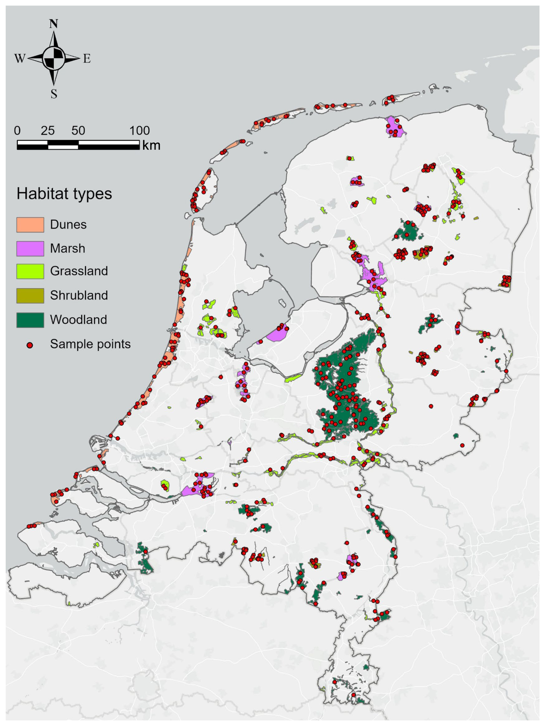
Figure A1 Natura 2000 sites and their habitat types in the Netherlands. The non-water habitat types were grouped into five classes (i.e. dunes, marshes, grasslands, shrublands, and woodlands) to conduct vegetation structure comparisons. For each class, we randomly sampled 100 plots (10 m × 10 m each) where Hp95 was not NA (assuming that vegetation occurs in the plots) for the analysis (n=500 in total).

The shapefile of the Natura 2000 sites within the Netherlands (with habitat class information in attributes), 100 sample plots for each habitat class, original and grouped habitat class information (.csv files), and the R processing script are provided in the data repository (see Sect. 6) and the code repository (see Sect. 7).

Appendix B

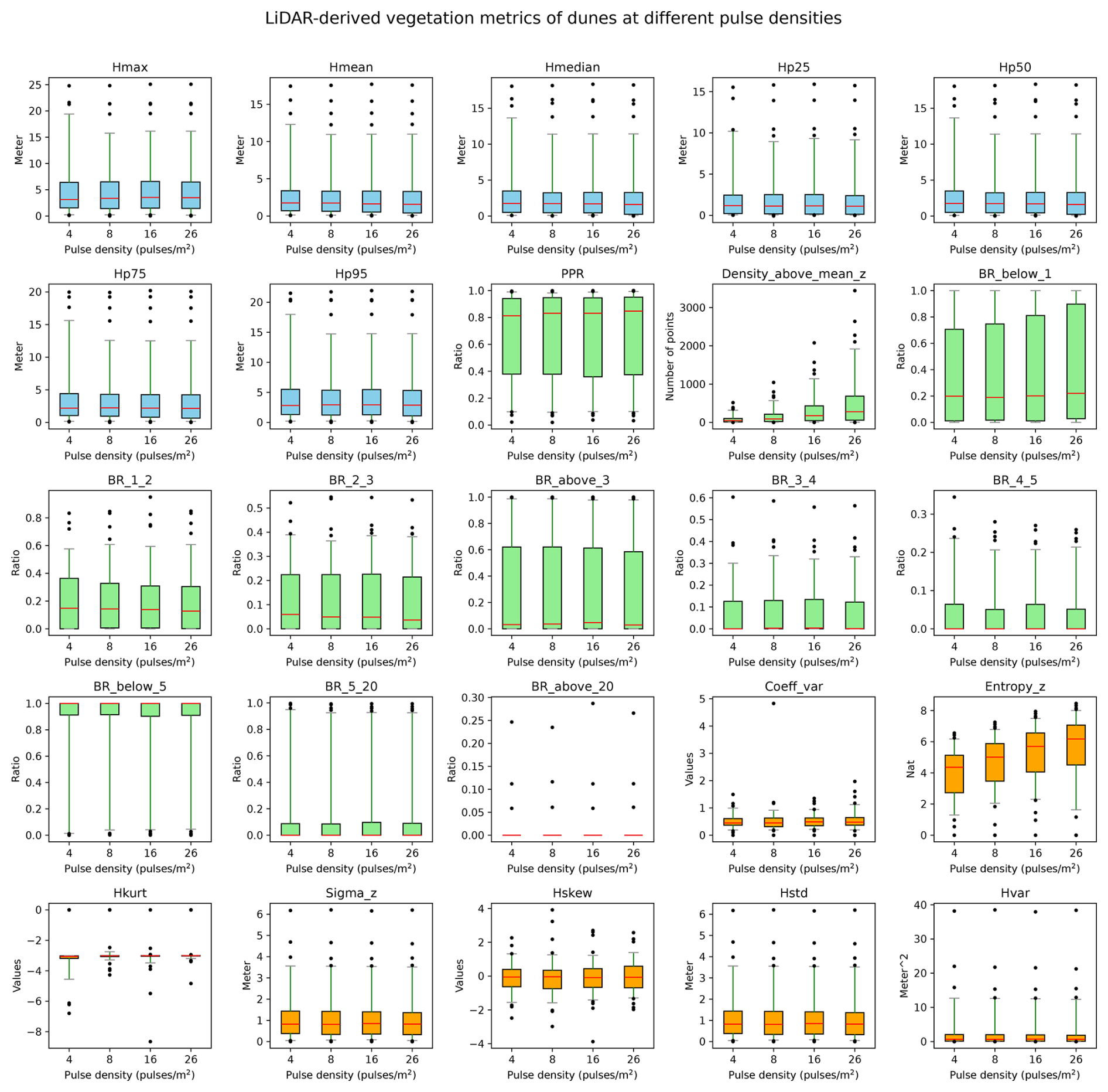
Figure B1 Robustness of vegetation metrics in dune habitats. A total of 25 lidar metrics (blue: vegetation height metrics, green: vegetation cover metrics, orange: vegetation structural variability metrics) were calculated with different pulse densities across 100 plots of 10×10 m resolution in dune habitats in the Netherlands. Pulse densities were systematically down-sampled based on their GPS time from the original AHN4 dataset to the pulse density of AHN3 and two lower pulse densities (i.e. one-half and one-quarter of the pulse density of AHN3 to represent AHN2 and AHN1, respectively). Boxes represent the interquartile range, horizontal red lines represent the medians, whiskers extend to the 5th and 95th percentiles, and outliers are plotted as dots. See Table 3 for metric explanations.

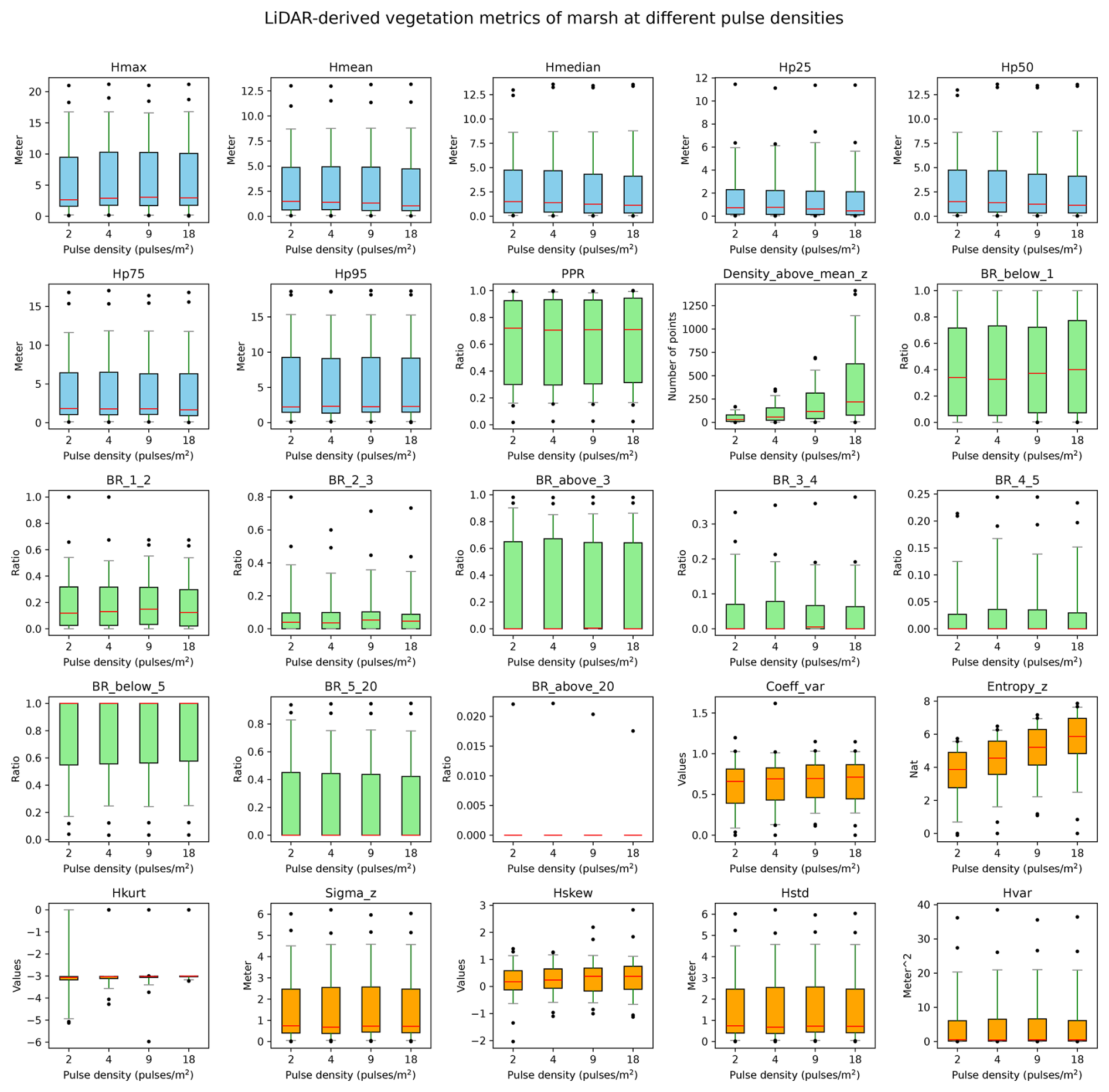
Figure B2 Robustness of vegetation metrics in marsh habitats. A total of 25 lidar metrics (blue: vegetation height metrics, green: vegetation cover metrics, orange: vegetation structural variability metrics) were calculated with different pulse densities across 100 plots of 10×10 m resolution in marsh habitats in the Netherlands. Pulse densities were systematically down-sampled based on their GPS time from the original AHN4 dataset to the pulse density of AHN3 and two lower pulse densities (i.e. one-half and one-quarter of the pulse density of AHN3 to represent AHN2 and AHN1, respectively). Boxes represent the interquartile range, horizontal red lines represent the medians, whiskers extend to the 5th and 95th percentiles, and outliers are plotted as dots. See Table 3 for metric explanations.

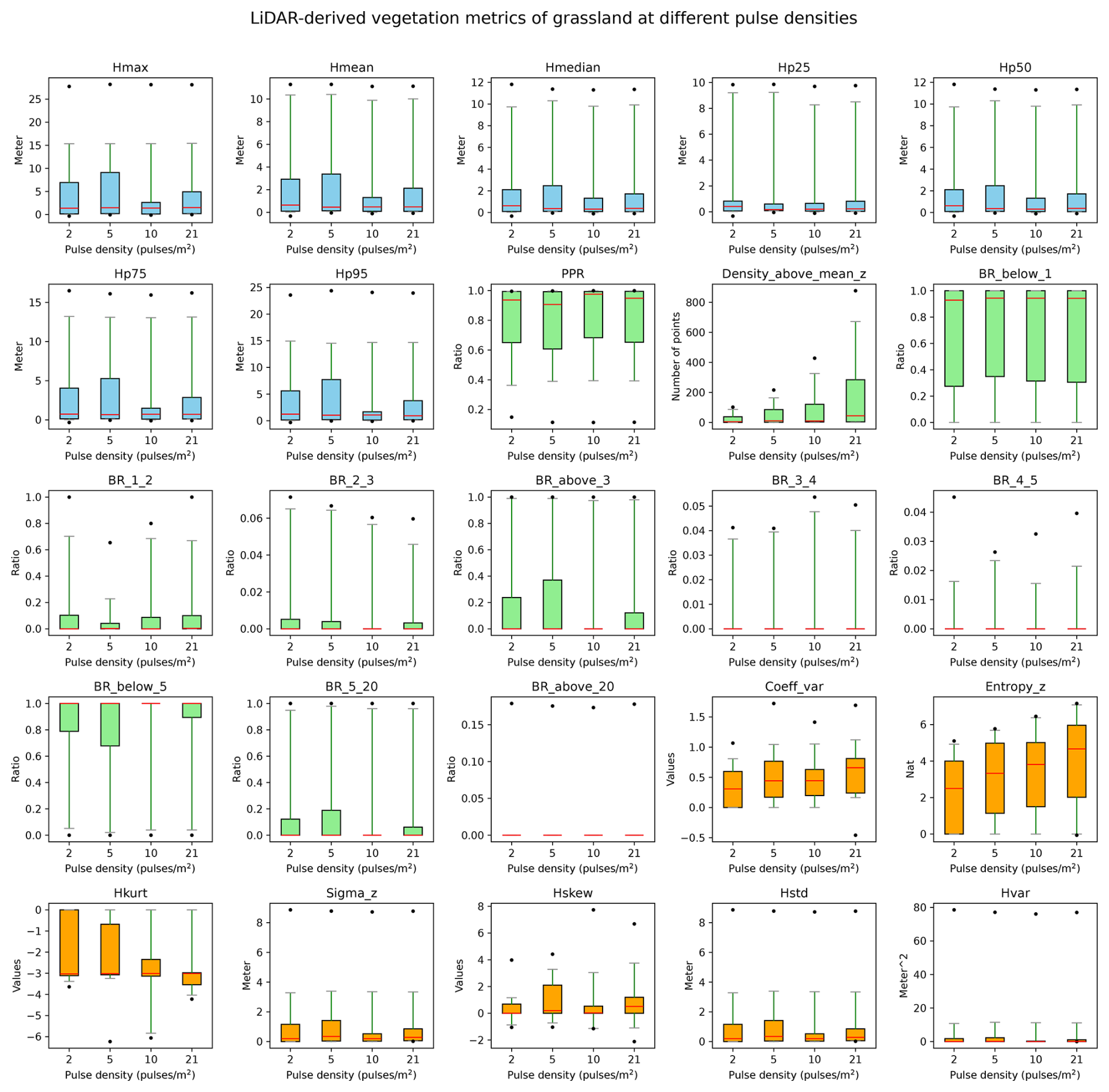
Figure B3 Robustness of vegetation metrics in grassland habitats. A total of 25 lidar metrics (blue: vegetation height metrics, green: vegetation cover metrics, orange: vegetation structural variability metrics) were calculated with different pulse densities across 100 plots of 10×10 m resolution in grassland habitats in the Netherlands. Pulse densities were systematically down-sampled based on their GPS time from the original AHN4 dataset to the pulse density of AHN3 and two lower pulse densities (i.e. one-half and one-quarter of the pulse density of AHN3 to represent AHN2 and AHN1, respectively). Boxes represent the interquartile range, horizontal red lines represent the medians, whiskers extend to the 5th and 95th percentiles, and outliers are plotted as dots. See Table 3 for metric explanations.

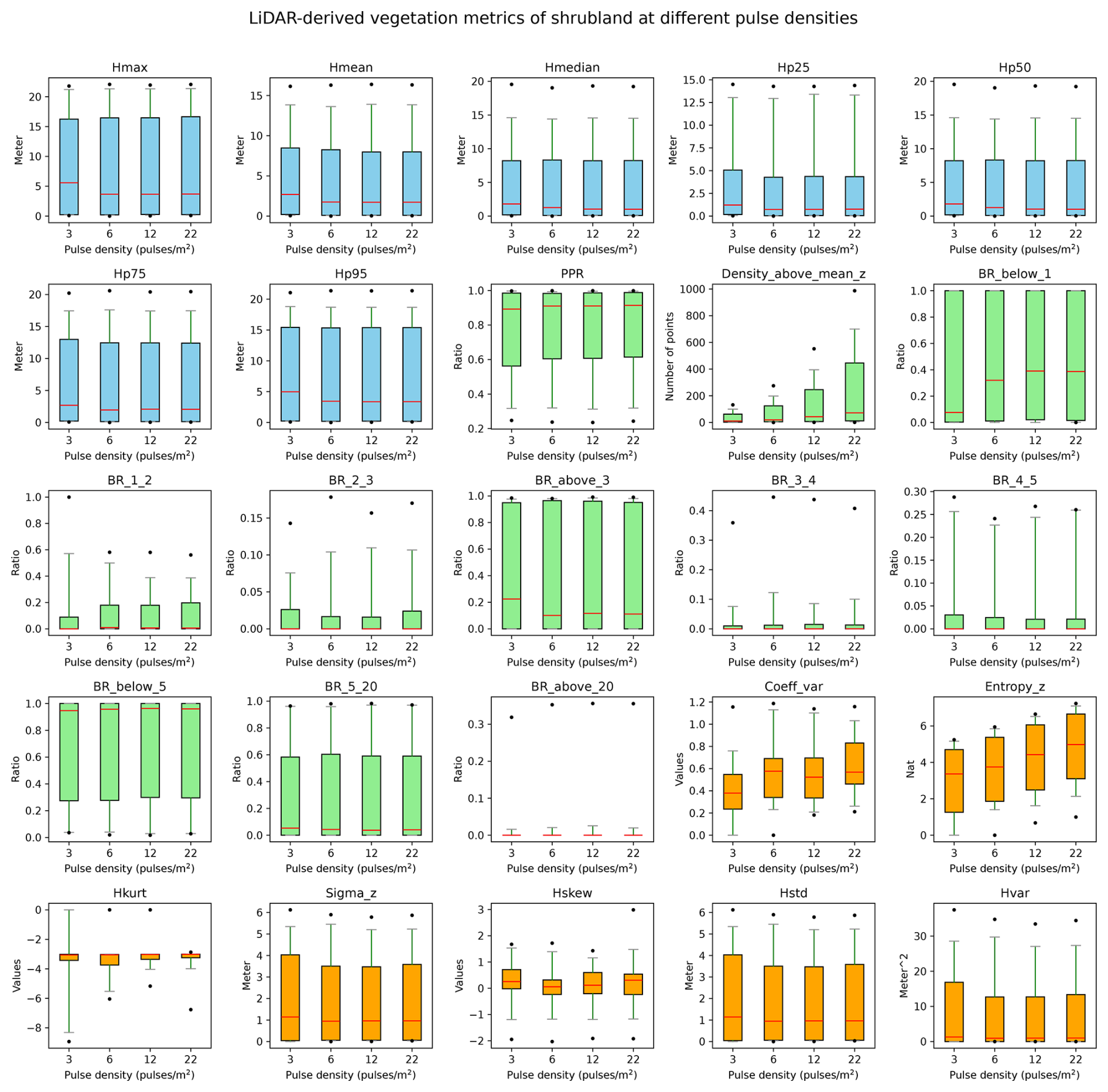
Figure B4 Robustness of vegetation metrics in shrubland habitats. A total of 25 lidar metrics (blue: vegetation height metrics, green: vegetation cover metrics, orange: vegetation structural variability metrics) were calculated with different pulse densities across 100 plots of 10×10 m resolution in shrubland habitats in the Netherlands. Pulse densities were systematically down-sampled based on their GPS time from the original AHN4 dataset to the pulse density of AHN3 and two lower pulse densities (i.e. one-half and one-quarter of the pulse density of AHN3 to represent AHN2 and AHN1, respectively). Boxes represent the interquartile range, horizontal red lines represent the medians, whiskers extend to the 5th and 95th percentiles, and outliers are plotted as dots. See Table 3 for metric explanations.

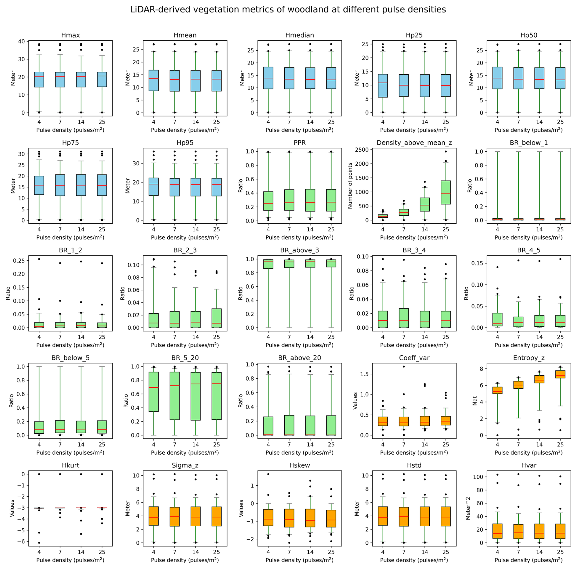
Figure B5 Robustness of vegetation metrics in woodland habitats. A total of 25 lidar metrics (blue: vegetation height metrics, green: vegetation cover metrics, orange: vegetation structural variability metrics) were calculated with different pulse densities across 100 plots of 10×10 m resolution in woodland habitats in the Netherlands. Pulse densities were systematically down-sampled based on their GPS time from the original AHN4 dataset to the pulse density of AHN3 and two lower pulse densities (i.e. one-half and one-quarter of the pulse density of AHN3 to represent AHN2 and AHN1, respectively). Boxes represent the interquartile range, horizontal red lines represent the medians, whiskers extend to the 5th and 95th percentiles, and outliers are plotted as dots. See Table 3 for metric explanations.

Appendix C

C1 Background

Since the methods and/or algorithms used in the pre-classification of the AHN datasets are unclear (no specific documents or information are publicly available) and because differences in pre-classification methods between AHN datasets can potentially lead to some biases in vegetation change detection (Fareed et al., 2023; Wu et al., 2019), we performed a preliminary assessment of the effect of terrain filtering on vegetation change detection across AHN datasets (i.e. AHN2–AHN4).

C2 Study area

The study area for this analysis is in the Amsterdam Water Supply Dunes (AWD), which is a 34 km² dune ecosystem in the west of Amsterdam, stretching 8 km along the Dutch North Sea coast, with a width varying from 1.5 to 5 km. The AWD area is dominated by various dune habitats, including shifting white dunes, fixed coastal dunes with herbaceous vegetation, dunes with sea buckthorn formations, wooded dunes, and humid dune slacks (Kissling et al., 2024b). Vegetation types include grasses (46 %), scrublands (22 %), forests (21 %), sand (6 %), and other low vegetation. To evaluate the impact of varying ground point classification approaches (for AHN2, AHN3, and AHN4) on derived lidar vegetation metrics, we selected three sample plots within the AWD area to conduct our analysis. We selected three sample areas (1 km × 1.3 km each) for this analysis, and the specific locations of each sample plots are as follows: area 1 – 52.304127° N, 5.437882° E; area 2 – 52.278998° N, 5.480002° E; and area 3 – 52.289103° N, 5.501239° E.

C3 Methods

First, we computed 25 lidar-derived vegetation metrics using the pre-classified AHN datasets (“unclassified” class) as in the main text. Second, we applied a filtering algorithm with identical parameter settings to the original multi-temporal AHN point clouds to reclassify the terrain and vegetation points consistently across AHN2–AHN4. We then derived the same 25 lidar metrics using the reclassified data, following the same workflow applied to the pre-classifications. All lidar metrics were derived and compared at a 10 m resolution. To further assess the differences in lidar-derived vegetation metric change across multi-temporal datasets, we conducted pairwise comparisons between AHN2 and AHN3 and between AHN3 and AHN4. The differences (delta metrics) were calculated by subtracting the vegetation metrics of the earlier datasets from those of the later ones (i.e. subtracting AHN2 from AHN3 and subtracting AHN3 from AHN4). The height of non-ground points was normalized using the height of the lowest point within each 1 m × 1 m grid cell (in line with the Laserfarm workflow). The resulting vegetation metrics were first exported as GeoTIFF files with a 10 m resolution, after which pixel-wise subtraction was performed.

We used an iterative grid-based filtering approach to segment terrain (i.e. ground) points from raw lidar point clouds, enabling efficient separation of vegetation and ground points in the dune environments. This filtering approach consists of four steps.

C3.1 Step 1: preprocessing

This step mainly removes the outliers of the original point cloud of AHN datasets. The statistical outlier removal (SOR) was employed to remove noise points with the method proposed in Rusu et al. (2008). Suppose that P is a set of 3D points, and, for each query point p_query∈P, $\stackrel{\mathrm{‾}}{d}$ is the mean distance of a query point to its k nearest neighbours. For all points in P, the mean distance and standard deviation of the distances of their k nearest neighbours are then determined. Only those points that have distances that are close to the mean distance of the closest neighbours are kept, using Eq. (C1).

$$\begin{array}{}\text{(C1)}& P^k=\left\{p_q\in P|\left({\mathit{\mu }}_k-\mathit{\alpha }{\mathit{\sigma }}_k\right)\le \stackrel{\mathrm{‾}}{d}\le \left({\mathit{\mu }}_k+\mathit{\alpha }{\mathit{\sigma }}_k\right)\right\}\end{array}$$

Here, α is a density threshold coefficient, and μ_k and σ_k are the mean and standard deviation of the distance from a query point to its k nearest neighbours. P^k is the point set that is kept, i.e. after removing the outliers.

C3.2 Step 2: grid initialization

The original 3D point cloud of the AHN is divided into a virtual grid layer, starting with a coarse resolution. The indices of the grids are calculated using Eq. (C2).

$$\begin{array}{}\text{(C2)}& n^i={\displaystyle \frac{P^i-P_{\min }^i}{{\mathrm{Size}}_{\mathrm{g}}^i}}(i\in x,y,z)\end{array}$$

Here, Pⁱ denotes the coordinates of a point, and size${}_{\mathrm{g}}^i$ is the grid size.

C3.3 Step 3: elevation interpolation

For each grid cell in the bottom layer, elevation E_g is interpolated using a distance-weighted average of points within the grid using Eq. (C3).

$$\begin{array}{}\text{(C3)}& E_{\mathrm{g}}={\displaystyle \frac{\sum E_{\mathrm{p}}\left(\frac{L}{\sqrt{\mathrm{2}}}-D_{\mathrm{g}}\right)}{\sum \left(\frac{L}{\sqrt{\mathrm{2}}}-D_{\mathrm{g}}\right)}}\end{array}$$

Here, L is the grid size, E_p is the elevation of a point, and D_g is the distance from the point to the geometric centre of the grid.

C3.4 Step 4: iterative refinement

The generated grids are iteratively subdivided by halving the grid size per iteration until reaching the minimum grid size. The points that exceed a height threshold above the interpolated terrain elevation are classified as vegetation points.

Finally, the original points are classified into terrain (i.e. ground) point and vegetation point categories. The classified vegetation and terrain points are applied to the computation of the lidar vegetation metrics. The parameter settings in this workflow were minimum grid size (1 m), maximum grid size (15 m), and height threshold (0.5 m).

C4 Results and conclusions

Our results revealed that the differences between the vegetation changes generated from point clouds using the AHN pre-classification and using a consistent terrain-filtering method across the AHN2–AHN4 datasets are negligible. The only exceptions were the pulse penetration ratio (PPR), the coefficient of variation of vegetation height (Coeff_var), and the Shannon index (Entropy_z), where small differences were observed (Figs. C1–C3). This analysis thus provides the first insights into the reliability of the pre-classification of the AHN datasets when calculating vegetation change. Conditional on those results, we conclude that most lidar metrics based on the pre-classifications of AHN (AHN2–AHN4) datasets are reliable, with only a few vertical variability metrics showing a detectable effect of potential differences in the ground classification methods between AHN2–AHN4 datasets. It should be noted that we conducted this assessment only in the Dutch coastal dunes, and similar assessments can be done across different sites and different habitats in future studies for a more comprehensive understanding of this topic.

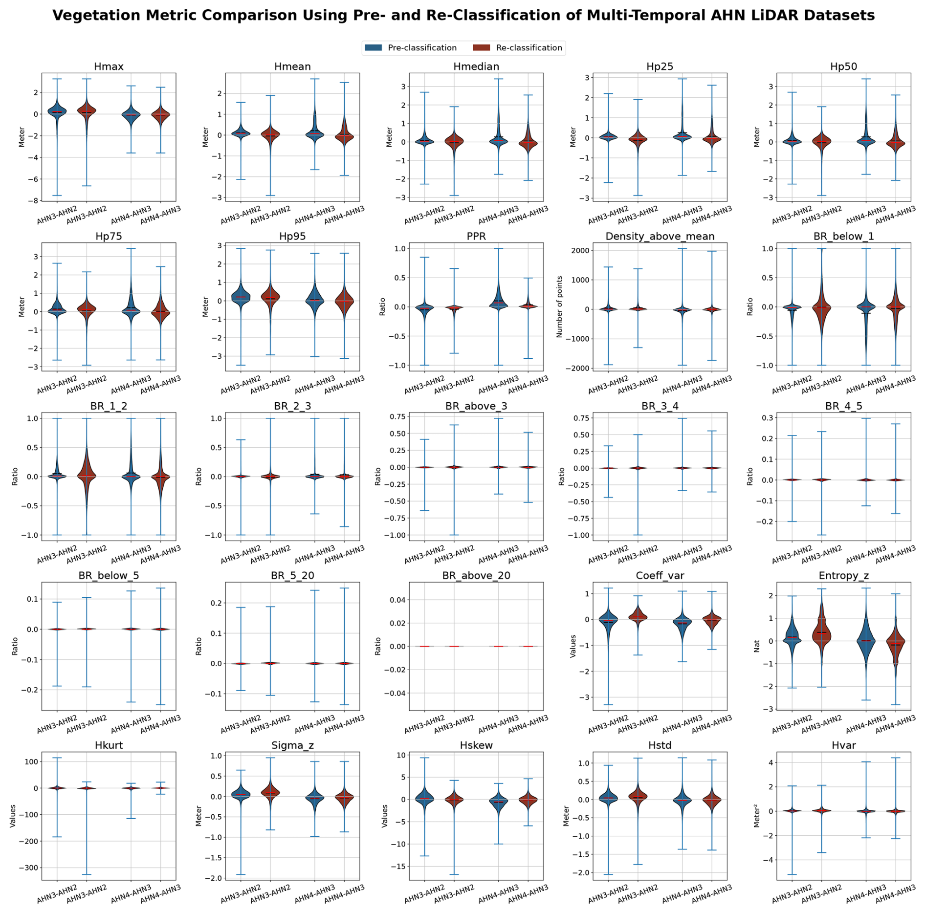
Figure C1 Pixel-wise comparisons of lidar-derived vegetation changes from area 1 using the pre-classifications from the AHN2–AHN4 datasets (blue) vs. those using a consistent terrain-filtering method across the three AHN datasets (red). The total number of pixels in area 1 is 13 416 (n=13 416).

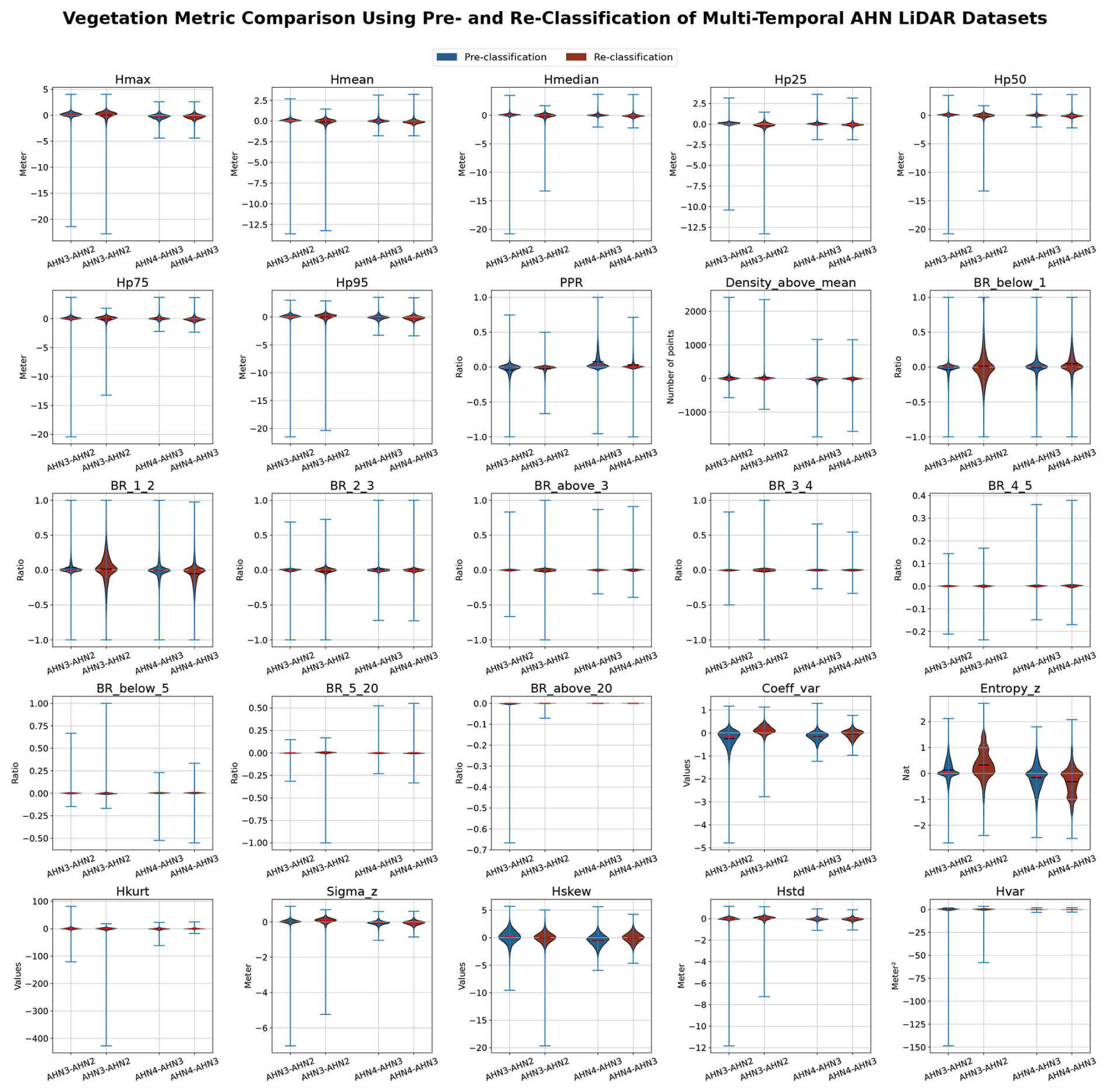
Figure C2 Pixel-wise comparisons of lidar-derived vegetation changes from area 2 using the pre-classifications from the AHN2–AHN4 datasets (blue) vs. those using a consistent terrain-filtering method across the three AHN datasets (red). The total number of pixels in area 2 is 13 416 (n=13 416).

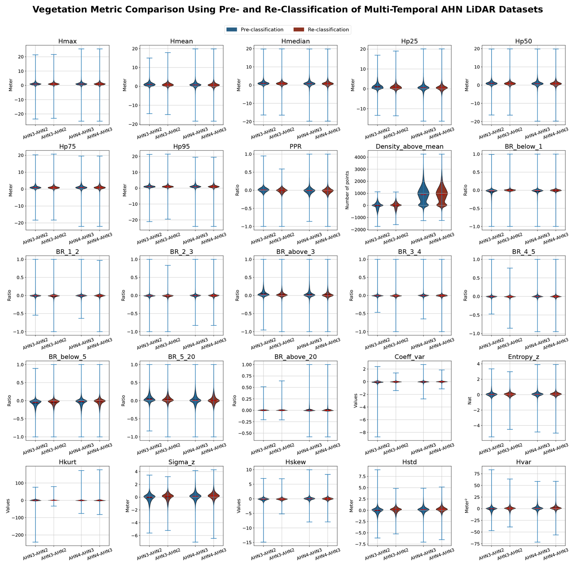
Figure C3 Pixel-wise comparisons of lidar-derived vegetation changes from area 3 using the pre-classifications from the AHN2–AHN4 datasets (blue) vs. those using a consistent terrain-filtering method across the three AHN datasets (red). The total number of pixels in area 3 is 13 416 (n=13 416).