Antarctic Ice Sheet grounding line discharge from 1996–2024

Grounding line discharge is a key component of the mass balance of the Antarctic Ice Sheet. Here, we present a time-varying estimate of Antarctic Ice Sheet grounding line discharge, at up to monthly intervals, from 1996 through to November 2024. We calculate ice flux through 16 algorithmically generated flux gates across 998 ice sheet, glacier, ice stream and ice shelf drainage basins. We draw on a range of ice velocity and thickness data to estimate grounding line discharge. For ice thickness, we use three bed topography datasets, two firn models and a time-varying ice surface. For the ice velocity, we utilise a range of publicly available ice velocity maps at resolutions ranging from 200 m×200 m to 1000 m×1000 m, as well as new 100 m×100 m monthly velocity mosaics derived from intensity tracking of Sentinel-1 image pairs, available since October 2014. Our dataset also includes the contributions to discharge from changes in ice thickness due to surface lowering, time-varying firn air content, and surface mass change between the flux gates and grounding line. We find that Antarctic Ice Sheet grounding line discharge increased from 1999±175 to $\mathrm{2224}\pm \mathrm{200}\mathrm{Gt}{\mathrm{yr}}^{-\mathrm{1}}$ between 1996 and 2024, much of which was due to the acceleration of ice streams in West Antarctica but with substantial contributions from ice streams in East Antarctica and glaciers on the Antarctic Peninsula. The errors in our discharge dataset stem approximately equally from errors in the underlying ice velocity and thickness measurements. However, we find that the spread in possible discharge estimates depending on the choice of bed topography dataset and flux gate location is much larger than the error in any single estimate. It is our intention to update this discharge dataset each month, subject to continued Sentinel-1 acquisitions and funding availability. The dataset is freely available at https://doi.org/10.5281/zenodo.10051893 (this paper was prepared using version 7 of the dataset) (Davison et al., 2024).

1 Introduction

The rate of mass loss from the Antarctic Ice Sheet has accelerated since the early 1990s (Otosaka et al., 2023; Diener et al., 2021; Slater et al., 2021; Shepherd et al., 2019). Mass loss has been the greatest and most rapid in West Antarctica, where ice streams draining into the Amundsen Sea embayment have accelerated dramatically during the satellite era (Mouginot et al., 2014; Konrad et al., 2017). As such, the majority of mass loss from the Antarctic Ice Sheet is attributed to increases in grounding line discharge – the flux of ice into ice shelves or directly into the Southern Ocean from the grounded Antarctic Ice Sheet (henceforth discharge). Discharge is therefore a key component for quantifying the “health” of the Antarctic Ice Sheet, particularly when combined with surface mass balance (SMB) estimates, to determine overall ice sheet mass change (Rignot et al., 2019; Sutterley et al., 2014). This mass budget or input–output approach to measuring ice sheet mass change complements other ice sheet mass change measurements derived from altimetry measurements (Smith et al., 2020; Shepherd et al., 2019) or gravimetric approaches (Diener et al., 2021; Velicogna et al., 2020; Sutterley et al., 2020). The principal benefits of the input–output method are twofold. Firstly, when combined with an estimate of steady-state SMB and discharge, it permits the partitioning of mass change between SMB and discharge, which provides an insight into the processes driving ice sheet mass change. Secondly, discharge is derived from ice velocity and thickness datasets, which can now be generated through continuous satellite-based monitoring at relatively frequent (∼monthly) intervals at the continent scale. These data are available at higher spatial resolution than the other mass change measurement approaches, making the input–output method particularly useful in smaller drainage basins and in mountainous terrain, where it is limited primarily by SMB model performance. Despite their utility, grounding line discharge measurements for Antarctica are relatively sparse (Rignot et al., 2019; Gardner et al., 2018; Miles et al., 2022; Depoorter et al., 2013), resulting in only one estimate of ice sheet mass change using the input–output method (Rignot et al., 2019; Otosaka et al., 2023; Shepherd et al., 2018), which means that independent verification of ice sheet mass balance using this method is lacking. Furthermore, the limited available discharge estimates disagree in some regions and basins (for example, the Antarctic Peninsula) such that opposing conclusions regarding basin-scale mass change must be reached for those basins (Hansen et al., 2021).

Here, we present a new grounding line discharge dataset for the Antarctic Ice Sheet. We draw on several bed topography products and velocity measurements from 1996 through to November 2024, and we use time-varying rates of ice surface elevation change and firn air content. The velocity measurements range in spatial resolution from 1 km×1 km annually to 100 m×100 m every month since October 2014, thereby increasing the detail and frequency of continent-wide discharge estimates over time. We provide these discharge estimates integrated over every published basin definition available for Antarctica – ranging in scale from the whole ice sheet down to 1 km wide glaciers on the Antarctic Peninsula. It is our intention to update this discharge dataset each month, subject to continued Sentinel-1 acquisitions and funding availability. In addition, we will endeavour to provide irregular updates following the release of new bed topography datasets or grounding lines and if any bugs are identified.

2 Data and methods

2.1 Bed topography, ice surface and ice thickness

We estimate grounding line discharge using multiple bed elevation datasets. Our primary estimates of bed elevation and bed elevation error draw predominantly on BedMachine v3 (Morlighem, 2020; Morlighem et al., 2020), but we replace the BedMachine bed and bed error with a dedicated bed topography dataset over the Antarctic Peninsula (Huss and Farinotti, 2014) after conversion to a common geoid (GL04c). We use the MATLAB tool wgs2gl04c to perform this conversion (Greene et al., 2019). Henceforth, we refer to this merged bed topography dataset as BM + HF14 (Figs. 1, A2 and A3). For comparison, we also provide discharge estimates using the bed topography data and associated error from BedMap2 (Fretwell et al., 2013).

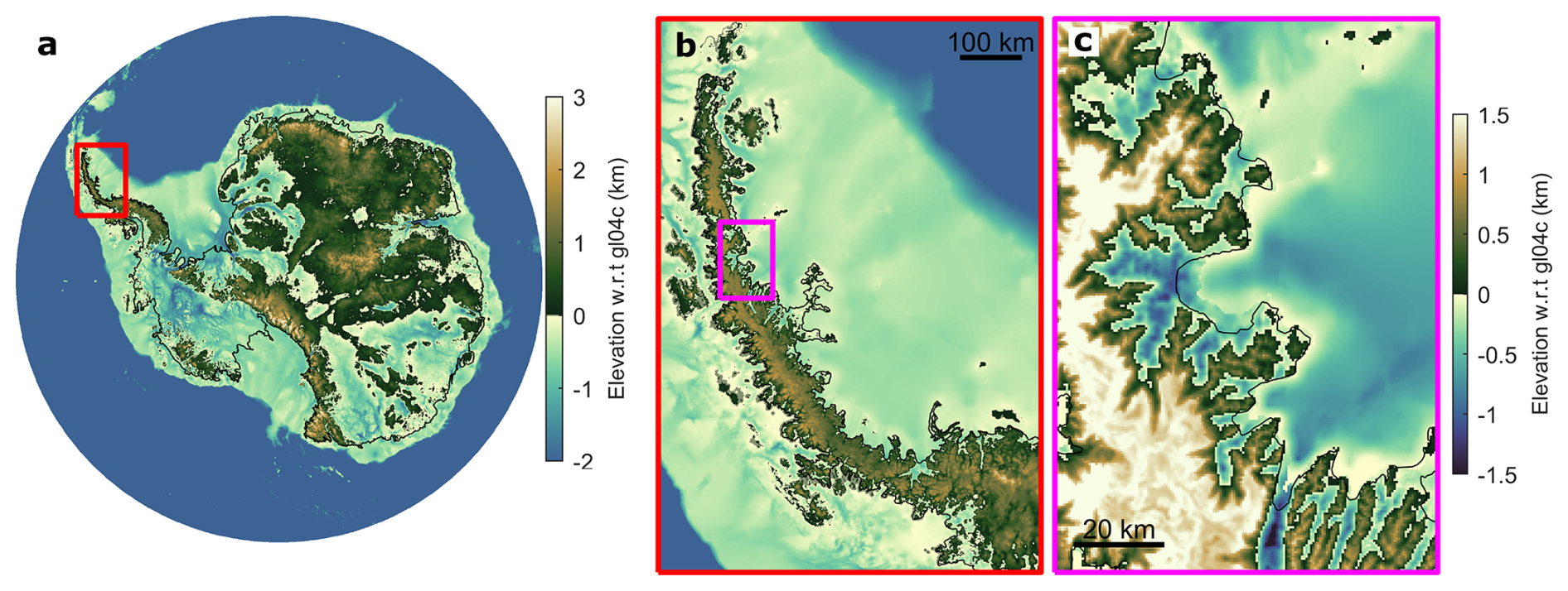
Figure 1 Antarctic Ice Sheet bed topography overview. (a) Overview of BedMachine v3. Also shown are overviews of (b) the Antarctic Peninsula (Huss and Farinotti, 2014) and (c) the Larsen B embayment with BM + HF14. The coastline and grounding line are shown as black lines.

For each of these bed products, we calculate ice thickness using the Reference Elevation Model of Antarctica (REMA) digital elevation model (DEM), posted at 100 m×100 m and timestamped to 9 May 2015 (Howat et al., 2019). Before calculating ice thickness, we reference the REMA DEM elevations to the GL04c geoid and remove the climatological mean (1979–2008) firn air content (Veldhuijsen et al., 2023) (Sect. 2.4). Henceforth, we refer to this firn-corrected ice surface as our reference ice surface, which we assume has a spatially uniform 1 m error (Howat et al., 2019). For the thickness grid calculated using BM + HF14, we fill exterior gaps through extrapolation along ice flowlines using the same method applied to the reference velocity map described in Sect. 2.3. The purpose of the extrapolation is to ensure that ice thickness estimates are available at each flux gate pixel (Sect. 2.4). We chose to extrapolate along flowlines rather than using a more conventional nearest-neighbour interpolation because the latter can lead to erroneous or poorly targeted sampling near shear margins. To generate an ice thickness time series from each of these baseline thickness estimates, we modify the REMA DEM using observed changes in ice surface elevation from 1992–2023 (Fig. A1) derived from satellite radar altimetry following the methods of Shepherd et al. (2019). Because satellite altimetry measurements do not fully observe the ice sheet margins at monthly intervals, we estimate monthly time series of ice surface elevation change by fitting time-dependent quadratic polynomials (Fig. A1) to the observed surface elevation changes posted on a 5 km×5 km grid at quarterly intervals, which we linearly interpolate to our gate pixels and evaluate at each velocity epoch (Sect. 2.3). We apply these modelled time series of elevation change to each reference ice thickness estimate to form time series of ice thickness at each gate pixel. We quantify the errors in the elevation change by calculating upper and lower bounds to the quadratic fit from the 95 % confidence interval on each of the model coefficients (Sect. 2.7.3). South of 81.5°, where elevation change measurements have only been available since the launch of CryoSat-2 in 2010, we assume static ice thickness rather than extrapolate the historical thinning rates from those observed between 2010 and 2023. Given that the flux gate pixels south of 81.5° only contribute 6 % to the pan-Antarctic discharge and that the applied thickness changes elsewhere around the continent only modify the total discharge by 0.7 %, this choice has little impact on our pan-Antarctic discharge estimate. We then account for temporal variations in firn air content by adjusting the climatological firn air content correction in each flux gate pixel using time series of firn air content anomalies from two firn models (Sect. 2.2) at each velocity epoch. For discharge estimates after the last available output from each firn model, we use the monthly firn air content climatology (1979–2008) in order to capture seasonal changes in firn air content. For discharge estimates after January 2023, when our thickness change observations end, we continue to use the quadratic fit. We also assume no changes in bed elevation due to erosion of the substrate or changes in ice thickness due to changes in subglacial melt rates, both of which are expected to be negligible.

2.2 Firn air content

We use two firn models (Fig. 2) to remove firn air content from our ice thickness estimates, to determine the ice equivalent thickness at each flux gate and to permit the use of a single ice density value in the discharge calculation (Sect. 2.7). These are the Institute for Marine and Atmospheric Research Utrecht Firn Densification Model (IMAU FDM) (Veldhuijsen et al., 2023) and the Goddard Space Flight Center FDM (GSFC-FDMv1.2), which draws on the Community Firn Model framework and is forced by the Modern-ERA Retrospective analysis for Research and Applications Version 2 (MERRA-2) climate forcing (Medley et al., 2022b, a). The resolution of the IMAU FDM is 27 km×27 km and of the GSFC-FDMv1.2 is 12.5 km×12.5 km. Both models provide daily firn air content for all of Antarctica and span the periods January 1979–December 2021 for the IMAU FDM and January 1980–July 2022 for GSFC-FDMv1.2. We use both solutions independently and provide a discharge estimate using each.

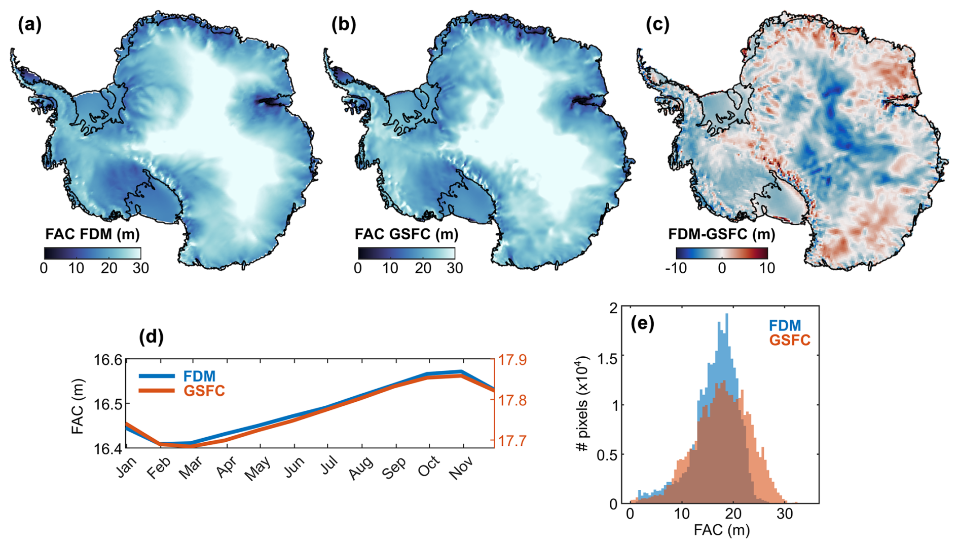
Figure 2 Overview of firn air content models. Overviews of (a) the IMAU FDM, (b) the GSFC-FDMv1.2 and (c) the difference between the two models. (d) The climatological seasonal cycle of firn air content (FAC) in each firn model. Note that in panel (d) the IMAU FDM and the GSFC-FDMv1.2 are plotted on separate y axes to facilitate comparison of their seasonal variability; their units are the same. (e) The frequency distribution of FAC at every flux gate pixel in each model.

2.3 Ice velocity

Prior to constructing an ice velocity and discharge time series, we generate a reference velocity grid in order to fill gaps in the time series velocity products. We construct the reference velocity grid by combining two velocity products. First, we use a 100 m×100 m multi-year velocity mosaic derived from feature tracking of Sentinel-1 imagery between January 2017 and September 2021 (Davison et al., 2023a). Sentinel-1 imagery is only continuously acquired around the Antarctic Ice Sheet margin, with sparser measurements further inland acquired in 2016. To fill the pole hole in the reference grid, we use the 450 m×450 m MEaSUREs reference velocity product (Rignot et al., 2017), which is linearly interpolated to the grid of the Sentinel-1 product. We fill interior gaps in this mosaic using the regionfill algorithm in MATLAB, which smoothly interpolates inward from the known pixel values on the outer boundary of each empty region by computing the discrete Laplacian over each region and solving the Dirichlet boundary value problem. This interior gap filling has no bearing on our discharge estimate, but it allows for easier filling of external gaps. We then fill exterior gaps through extrapolation along flowlines following the method of Greene et al. (2022), where the observed velocity is multiplied by the observed thickness mosaic (described in Sect. 2.1), before extrapolating along the hypothetical direction of flow and inpainting between flowlines. We multiply the ice velocity by the reference ice thickness before extrapolating and inpainting so as to give appropriate weight to flow directions of thicker ice that contribute more to ice flux. As with the reference thickness map, we choose to extrapolate along flowlines to avoid erroneous sampling of ice velocity, especially near shear margins. This produces a gapless ice velocity map of Antarctica (Fig. 3), broadly representing the average velocity of the ice sheet from 2015–2021. We emphasise that the purpose of the gap filling is only to ensure that a velocity estimate is available at every flux gate pixel. As such, the velocity in the ice sheet interior and the extrapolated velocity seaward of the flux gates in this reference map have no bearing on our discharge estimate.

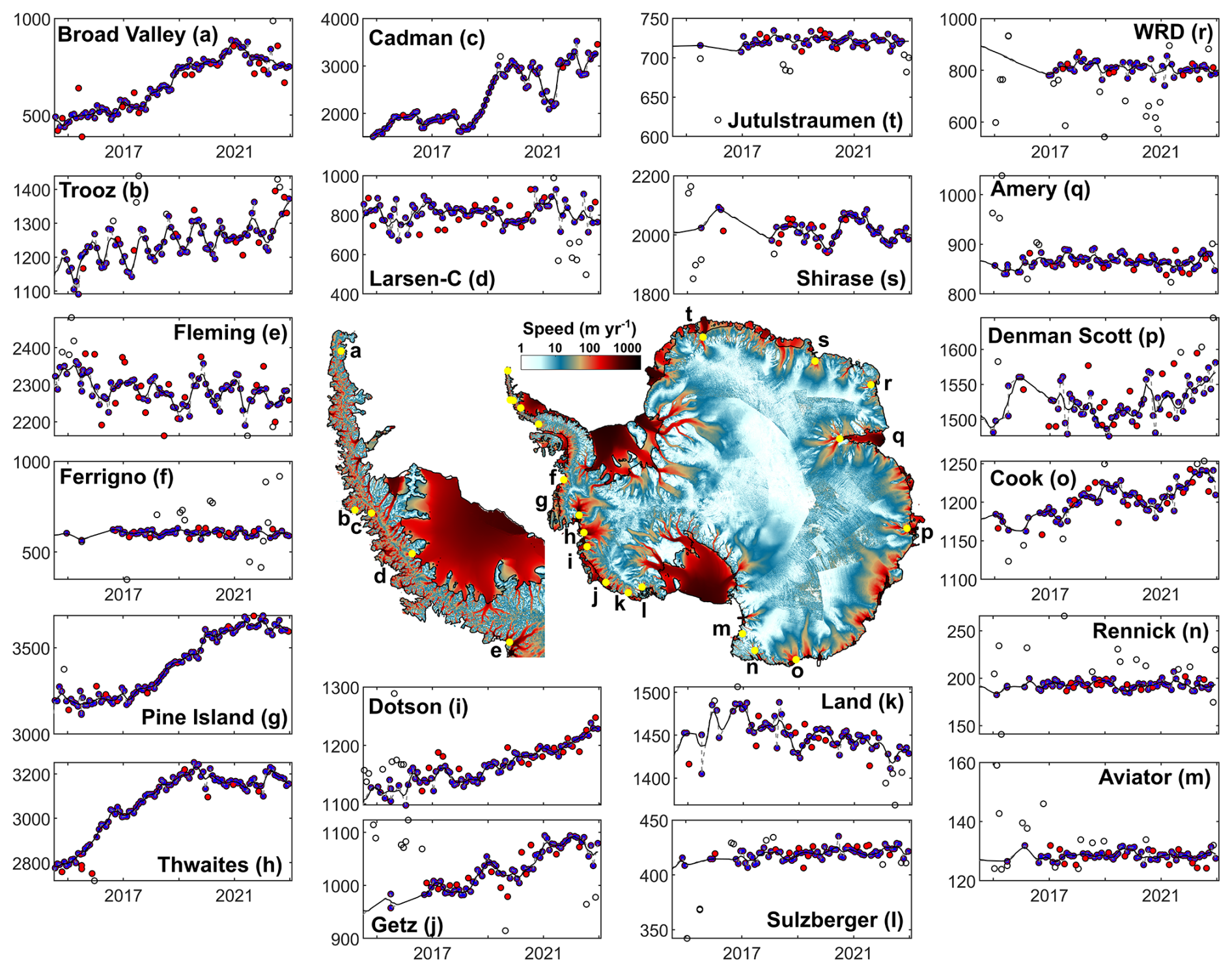
Figure 3 Reference ice velocity map and time series, with outlier removal. The central plot shows the reference ice velocity map (with extrapolated velocities masked to aid visualisation). Panels (a)–(t) show example time series of cross-gate velocity (in m yr⁻¹) extracted from single flux gate pixels. The black circles show points removed by the global outlier filters, and the red dots show points removed by the local outlier filters. The unsmoothed filled time series is shown as a dashed grey line, and the smoothed time series is shown as a black line. WRD is Wilma Robert Downer.

For our time series product, we compile multiple velocity sources:

1. the 1 km×1 km MEaSUREs annual velocity mosaics (Mouginot et al., 2017b, a) for the year 2000 and from 2005–2016;

2. monthly 100 m×100 m velocity mosaics derived from intensity tracking of Sentinel-1 image pairs (described in Appendix A), available from October 2014–November 2024 (Davison et al., 2023b, a);

3. monthly 200 m×200 m velocity mosaics derived from intensity and coherence tracking of Sentinel-1 image pairs, available from October 2014–December 2021 (Nagler et al., 2015).

4. in the Amundsen Sea embayment in 1996, we also use a combination of 450 m×450 m MEaSUREs InSAR-based velocities derived from 1 d repeat ERS-1 imagery (Rignot et al., 2014), which covers the region spanning Cosgrove to Kohler Glacier, and 200 m×200 m velocities from ERS-1 offset tracking over the Getz Basin (https://cryoportal.enveo.at/data/, last access: 6 March 2024), where the latter had been filled using an optimisation procedure supported by the BISICLES ice sheet model (Selley et al., 2021).

5. the 240 m×240 m ITS_LIVE annual mosaics (Gardner et al., 2019) during 1996–2018;

6. two 450 m×450 m MEaSUREs multi-year velocity mosaics, which incorporate velocity estimates in the periods 1995–2001 and 2007–2009 (Rignot et al., 2022);

7. in the Amundsen Sea embayment, gap-filled 240 m×240 m ITS_LIVE annual mosaics from 1996–2018 (Paolo et al., 2023; Gardner, 2023);

8. over Pine Island Glacier, 500 m×500 m mosaics of ice velocity derived from speckle tracking of TerraSAR-X and TanDEM-X imagery, averaged over 2–5-month periods from 2009–2015 (Joughin et al., 2021).

Each of these velocity products spans a time period; following Mankoff et al. (2019, 2020), we treat each product as an instantaneous measurement with the timestamp given by the central date in the estimate.

From these data, we generate discharge-ready gapless velocity time series at up to monthly temporal resolution at each gate pixel as follows. We linearly interpolate the easting and northing velocities and their respective errors from each product to each flux gate pixel. There are differences between velocity data sources that we assume are related to differences in the spatial resolution of the input satellite datasets, offset tracking parameter choices, digital elevation models used in the tracking, image co-registration procedures, outlier removal routines and final dataset posting. The differences between data sources at similar time periods are often the greatest in ice stream shear margins and are not consistent around Antarctica. Treating each gate pixel as a time series, we first remove extreme outliers defined as points more than 2 times or less than half of the reference velocity. We reduce the differences between data sources by applying a five-point moving-mean filter prior to the Sentinel-1 period and then a 3-month window thereafter to the raw velocities. This approach has the benefits of preferentially weighting data sources that provide similar velocity estimates within each window and does not require choosing a master data source with which to align the others. The differences between data sources and the effect of the alignment are detailed more in Appendix B.

Treating each flux gate pixel as a time series, we remove outliers in two stages. Firstly, we remove global time series outliers after detrending using two passes of a scaled median absolute deviation filter with thresholds of five and then three. This global filter is only applied to time series with more than 30 % of non-NaN measurements. Secondly, we remove local outliers using two passes of a moving median filter with a threshold of 2 median absolute deviations and window sizes of 4 months and then 3 months.

We fill gaps in each of our flux gate velocity time series in three stages. Firstly, we linearly interpolate across short temporal gaps (2 months or less). Secondly, we linearly interpolate across short spatial gaps (three gate pixels or fewer). Thirdly, we fill remaining temporal gaps using linear interpolation followed by back- and forward filling at the ends of each time series. The forward-filling of the velocity time series is used on all flux gate pixels south of 81.8° during the Sentinel-1 era, which contribute 6.2 % to our Antarctic-wide discharge. For gate pixels with no data at any time and more than three gate pixels from neighbouring finite pixels (after outlier removal), we use our reference ice velocity estimate, which has no gaps by definition. This final step affects just 0.05 %–0.15 % of flux gate pixels. After infilling, we smooth each pixel-based time series with two passes of a moving mean filter with window sizes of 3 months and then 4 months. Where we had removed outliers then infilled the time series, we set the easting and northing error to be $\left|\mathrm{10}\mathit{\%}\right|$ of the interpolated and smoothed easting and northing velocity components, respectively, at the gate pixel and velocity epoch in question. As in previous studies (Rignot et al., 2019; Gardner et al., 2018; Mankoff et al., 2019, 2020; Mouginot et al., 2014), we assume plug flow i.e. the depth-averaged velocity is the same as the measured surface velocity. Examples of our outlier removal and infilling are shown in Fig. 3.

2.4 Flux gates

We algorithmically generate 16 flux gates close to the Antarctic Ice Sheet grounding line (Fig. 4). Each flux gate is continuous around the Antarctic Ice Sheet and Wilkins Island; other Antarctic islands are not included in this analysis. The seaward grounding line is placed 3 years of ice flow upstream of the MEaSUREs grounding line (Mouginot et al., 2017c). The ice velocity for this migration is taken from the reference velocity dataset (described in Sect. 2.3), and the migration is performed in increments of 0.1 years to account for variations in ice velocity along the migration path. Gate pixels are spaced every 100 m for ice flowing faster than 100 m yr⁻¹ and 200 m for slower ice, defined on a polar stereographic grid (EPSG 3031) and accounting for distance distortions introduced by that projection. In total, 15 additional gates are generated at 200 m increments further upstream of the first gate such that the most upstream gate is 3 km upstream of the first gate. We provide discharge and error estimates for each of these flux gates and for the mean of all of the gates, weighted by the reciprocal of the error at each gate.

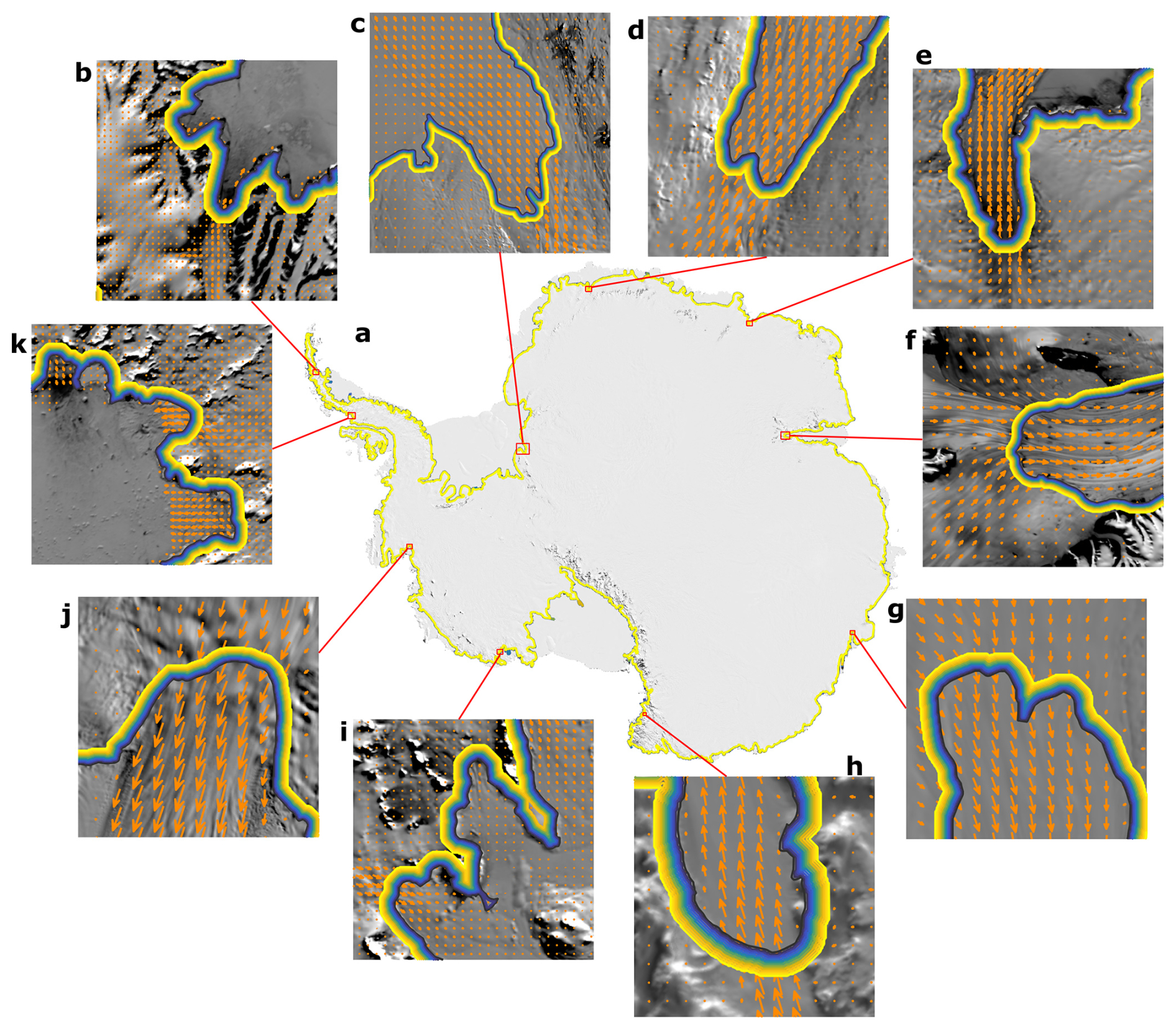
Figure 4 Flux gate overview. (a) Overview of Antarctica with flux gates plotted, where yellow lines represent the most inland gate and the blue lines represent the most seaward flux gate. Panels (b)–(k) show zoomed-in examples of the 16 flux gates in small regions around Antarctica, with ice velocity vectors overlain (orange arrows). The background image is the MODIS Mosaic of Antarctica (Scambos et al., 2007; Haran et al., 2021).

2.5 Mass change between flux gates and grounding line

Mass changes occur between each flux gate and the grounding line due to surface processes and due to subglacial melting. Here, we estimate mass changes due to surface processes only. We estimate this mass change for each drainage basin (Sect. 2.6) by integrating the climatological (1979–2008) surface mass balance from three regional climate models: RACMO2.3p2 (van Wessem et al., 2018), MAR (Agosta et al., 2019; Kittel et al., 2018) and HIRHAM5 (Hansen et al., 2021) in the area enclosed between each flux gate and the MEaSUREs grounding line (Mouginot et al., 2017c). This mass correction is applied at each velocity epoch. Since surface mass balance is generally positive downstream of the flux gates, this correction increases our Antarctic-wide grounding line discharge by 64 Gt yr⁻¹ on average.

2.6 Drainage basins

We provide a discharge estimate for all available Antarctic Ice Sheet drainage basins (Fig. 5). This includes the MEaSUREs regional basins and MEaSUREs glacier basins (Mouginot et al., 2017c), Zwally basins (Zwally et al., 2012), ice shelf basins (Davison et al., 2023a), and Antarctic Peninsula basins (Cook et al., 2014). In total, there are 998 drainage basins used in this study. For each basin, we provide the discharge through each of the 16 flux gates and the average of all flux gates (weighted by the reciprocal of their respective errors) along with their errors. These metrics are provided using each of the three bed topography estimates and with two firn models. In total, therefore, we provide 136 discharge time series for each basin. In addition, we provide the impact of the two ice thickness corrections – (1) IMAU FDM firn air content and (2) ice surface elevation changes – as well as the impact of downstream surface mass balance on each basin-integrated discharge estimate for each flux gate.

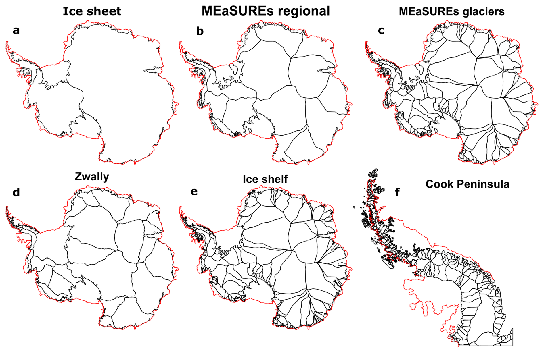
Figure 5 Overview of Antarctic Ice Sheet drainage basins. (a) Main ice sheet basins – East Antarctica, West Antarctica and the Antarctic Peninsula. Also shown are smaller drainage basin definitions, including (b) the MEaSUREs regional basins (Mouginot et al., 2017c), (c) the MEaSUREs glacier basins (Mouginot et al., 2017c), (d) the Zwally basins (Zwally et al., 2012), (e) the ice shelf basins (Davison et al., 2023a) and (f) the peninsula glacier basins (Cook et al., 2014). The coastline (Mouginot et al., 2017c) is shown in red.

2.7 Grounding line discharge

2.7.1 Balance discharge

We define the balance discharge as the discharge required to maintain the mass of a given ice sheet basin on long timescales (decades). In order to maintain the mass of a basin, the hypothetical balance discharge would therefore need to equal the basin-integrated SMB input on average. Accordingly, we estimate the balance discharge of each basin by integrating the 1979–2008 SMB from the mean of three regional climate models (RACMO2.3p2, MAR and HIRHAM5) within each of the above basins. We estimate the balance discharge error in each basin as the standard deviation of 10 realisations of 20-year climatologies from 1979–2008 (i.e. 1979–1999, 1980–2000, etc.). Note that only RACMO2.3p2 is available in 1979.

2.7.2 Discharge

We estimate grounding line discharge, D, across each flux gate pixel as

$$\begin{array}{}\text{(1)}& D=VHw\mathit{\rho },\end{array}$$

where V is the depth-averaged gate-normal ice velocity (assumed to be equal to the surface velocity), H is the ice equivalent thickness, w is the pixel width and ρ is ice density (917 kg m⁻³). This is an upper bound on bulk ice density and does not account for the effect of crevasses lowering ice density near the grounding line. The effect of ice density on discharge is linear, so reducing ice density to, for example, 900 kg m⁻³ would reduce our grounding line discharge estimate by approximately 2 %.

The gate-normal ice velocity is given by

$$\begin{array}{}\text{(2)}& V=\sin \left(\mathit{\theta }\right)V_x-\cos \left(\mathit{\theta }\right)V_y,\end{array}$$

where V_x and V_y are the easting and northing components of the horizontal ice velocity, as defined by the south polar stereographic grid (EPSG 3031), respectively, and θ is the angle of the flux gate relative to the same grid. To calculate the total discharge from each basin at each velocity measurement epoch, we simply sum the discharge through each flux gate pixel contained within the basin.

2.7.3 Discharge error

The uncertainties in our grounding line discharge stem primarily from errors in the ice velocity and ice thickness estimates. We calculate the cross-gate velocity uncertainty, V_σ, at each pixel and measurement epoch from the errors in the easting and northing velocity components:

$$\begin{array}{}\text{(3)}& \begin{array}{rl}{\displaystyle }& {\displaystyle }{V}_{x_{max}}=\sin \left(\mathit{\theta }\right)(V_x+V_{x_{\mathit{\sigma }}})-\cos \left(\mathit{\theta }\right)V_y,\\ {\displaystyle }& {\displaystyle }{V}_{x_{min}}=\sin \left(\mathit{\theta }\right)(V_x-V_{x_{\mathit{\sigma }}})-\cos \left(\mathit{\theta }\right)V_y,\\ {\displaystyle }& {\displaystyle }{V}_{y_{max}}=\sin \left(\mathit{\theta }\right)V_x-\cos \left(\mathit{\theta }\right)(V_y+V_{y_{\mathit{\sigma }}}),\\ {\displaystyle }& {\displaystyle }{V}_{y_{min}}=\sin \left(\mathit{\theta }\right)V_x-\cos \left(\mathit{\theta }\right)(V_y-V_{y_{\mathit{\sigma }}}),\\ {\displaystyle }& {\displaystyle }{V}_{\mathit{\sigma }}=\sqrt[\mathrm{2}]{(V-V_{x_{max}}{)}^{\mathrm{2}}+(V-V_{x_{min}}{)}^{\mathrm{2}}+(V-V_{y_{max}}{)}^{\mathrm{2}}+(V-V_{y_{min}}{)}^{\mathrm{2}}},\end{array}\end{array}$$

where $V_{x_{\mathit{\sigma }}}$ and $V_{y_{\mathit{\sigma }}}$ are the errors in the easting and northing component of the ice velocity, respectively.

The thickness uncertainty, H_σ, at each measurement epoch and gate pixel is calculated as

$$\begin{array}{}\text{(4)}& H_{\mathit{\sigma }}=\sqrt[\mathrm{2}]{(B_{\mathit{\sigma }}+\mathrm{1}{)}^{\mathrm{2}}+F_{\mathit{\sigma }}^{\mathrm{2}}+\mathrm{\Delta }{H}_{\mathit{\sigma }}^{\mathrm{2}}},\end{array}$$

where B_σ is the bed elevation error, taken from the respective bed elevation products, to which we add 1 m of ice surface elevation error (Howat et al., 2019). F_σ is the error in the firn air content correction, which we assume is 10 % of the correction. ΔH_σ is the error in the applied surface elevation change time series, which we calculate as follows:

$$\begin{array}{}\text{(5)}& \begin{array}{rl}{\displaystyle }& {\displaystyle }\mathrm{\Delta }{H}_{max}=t(a+a_{\mathit{\sigma }}{)}^{\mathrm{2}}+t(b+b_{\mathit{\sigma }})+(c+c_{\mathit{\sigma }}),\\ {\displaystyle }& {\displaystyle }\mathrm{\Delta }{H}_{min}=t(a-a_{\mathit{\sigma }}{)}^{\mathrm{2}}+t(b-b_{\mathit{\sigma }})+(c-c_{\mathit{\sigma }}),\\ {\displaystyle }& {\displaystyle }\mathrm{\Delta }{H}_{\mathit{\sigma }}=\left({\displaystyle \frac{{\mathit{\lambda }}_{\mathrm{1}}}{{\mathit{\lambda }}_{\mathrm{0}}}}\right)\left({\displaystyle \frac{(\mathrm{\Delta }{H}_{max}-\mathrm{\Delta }H)+(\mathrm{\Delta }H-\mathrm{\Delta }{H}_{\text{min}})}{\mathrm{2}}}\right).\end{array}\end{array}$$

Here, a, b and c are the quadratic, linear and intercept coefficients of the quadratic fit to the ice surface elevation change data. a_σ, b_σ and c_σ provide the bounds on the 95 % confidence interval for each coefficient. λ₀ and λ₁ are the sampling frequency of the fit (monthly) and the original observations (every 140 d) on which the fit is based, which together provide a scaling factor that prevents the uncertainty in ΔH scaling with the observational frequency.

Using the uncertainties in ice velocity and ice thickness described above, we calculate the velocity component of the discharge error, $D_{{\text{vel}}_{\mathit{\sigma }}}$, and the thickness component of the discharge error, $D_{H_{\mathit{\sigma }}}$, at each flux gate pixel and each measurement epoch. Both components of the discharge error are calculated in a Monte Carlo approach with 100 iterations. In each iteration, the timestamped cross-gate velocity and thickness in each pixel are separately modified using uniformly distributed random numbers generated from the timestamped and pixel-based cross-gate velocity and thickness errors. This produces 200 estimates of grounding line discharge at each measurement epoch and each flux gate pixel: 100 using the range of possible ice velocity values and 100 using the range of possible thickness values. The standard deviation of resulting timestamped pixel-based discharge estimates amongst each set of 100 iterations is taken as the velocity and thickness components of the discharge error.

We define our discharge error, D_σ, in each flux gate pixel and each measurement epoch, which is calculated as

$$\begin{array}{}\text{(6)}& D_{\mathit{\sigma }}=\sqrt[\mathrm{2}]{D_{{\text{vel}}_{\mathit{\sigma }}}^{\mathrm{2}}+D_{H_{\mathit{\sigma }}}^{\mathrm{2}}}.\end{array}$$

We calculate the basin-integrated discharge error, $D_{{\text{basin}}_{\mathit{\sigma }}}$, in two ways. Firstly, we follow Mankoff et al. (2019, 2020) and set the basin-integrated discharge error as the mean difference between the central discharge estimate and minimum and maximum possible discharge implied by the thickness and velocity errors described above:

$$\begin{array}{}\text{(7)}& D_{{\text{basin}}_{\mathit{\sigma }}}={\displaystyle \frac{(D_{max}-D)+(D-D_{min})}{\mathrm{2}}}.\end{array}$$

These errors are typically 7 % to 13 % of the basin-integrated discharge, and, because they accumulate the error in every pixel, they represent an upper bound on the discharge error. Secondly, we also provide the 95 % confidence interval of the gate-mean discharge based on the standard error in the discharge estimates through each of the 16 flux gates. The latter approach provides a measure of the uncertainty in the discharge estimate associated with the gate location, which in turn reflects the errors in the underlying ice velocity and ice thickness datasets and is typically less than 5 % of the basin-integrated discharge. In the following, all statistics use the former upper-bound estimate of discharge error, whilst plots use the latter estimate to facilitate visualisation of discharge changes.

3 Results

3.1 Grounding line discharge

We provide grounding line discharge estimates through 16 flux gates using 3 bed topography products and 2 firn models for 998 drainage basins. In the following, we primarily present values from the mean of all flux gates (weighted by the reciprocal of their errors) using our favoured bed topography dataset (BM + HF14) and the IMAU FDM. We also present comparisons across gates, bed topography datasets and firn models in turn.

Our primary discharge dataset (Fig. 6) gives a total Antarctic grounding line discharge of $\mathrm{1999}\pm \mathrm{175}\mathrm{Gt}{\mathrm{yr}}^{-\mathrm{1}}$ in 1996, rising to $\mathrm{2224}\pm \mathrm{200}\mathrm{Gt}{\mathrm{yr}}^{-\mathrm{1}}$ in 2024. On average, Antarctic discharge has increased at a rate of 8.7 Gt yr⁻² or 0.4 %yr⁻¹ over the study period from 1996. Our dataset shows that Antarctic grounding line discharge has not risen at a constant rate during our study period. Discharge increased steadily from 1998–2012 and has been increasing since 2016. These periods of rising discharge were interrupted by a period of gently declining discharge.

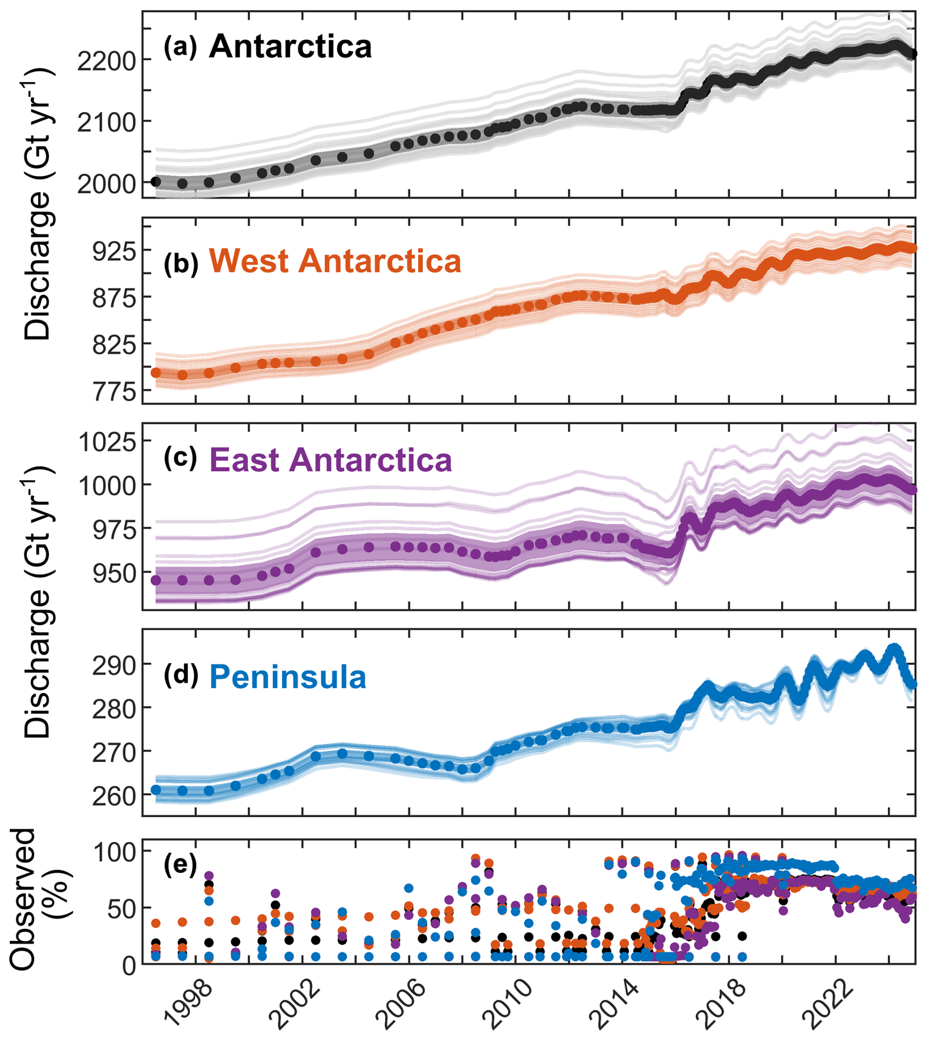
Figure 6 Antarctic Ice Sheet grounding line discharge. Discharge time series for (a) Antarctica, (b) West Antarctica, (c) East Antarctica and (d) the Antarctic Peninsula. In each panel, the dots show the central discharge estimate with 95 % confidence bounds (shading) and the discharge through each individual flux gate (faint lines). (e) The proportion of discharge that is observed, as opposed to infilled, shown for the whole Antarctic Ice Sheet (black dots), West Antarctica (orange dots), East Antarctica (purple dots) and the Antarctic Peninsula (blue dots).

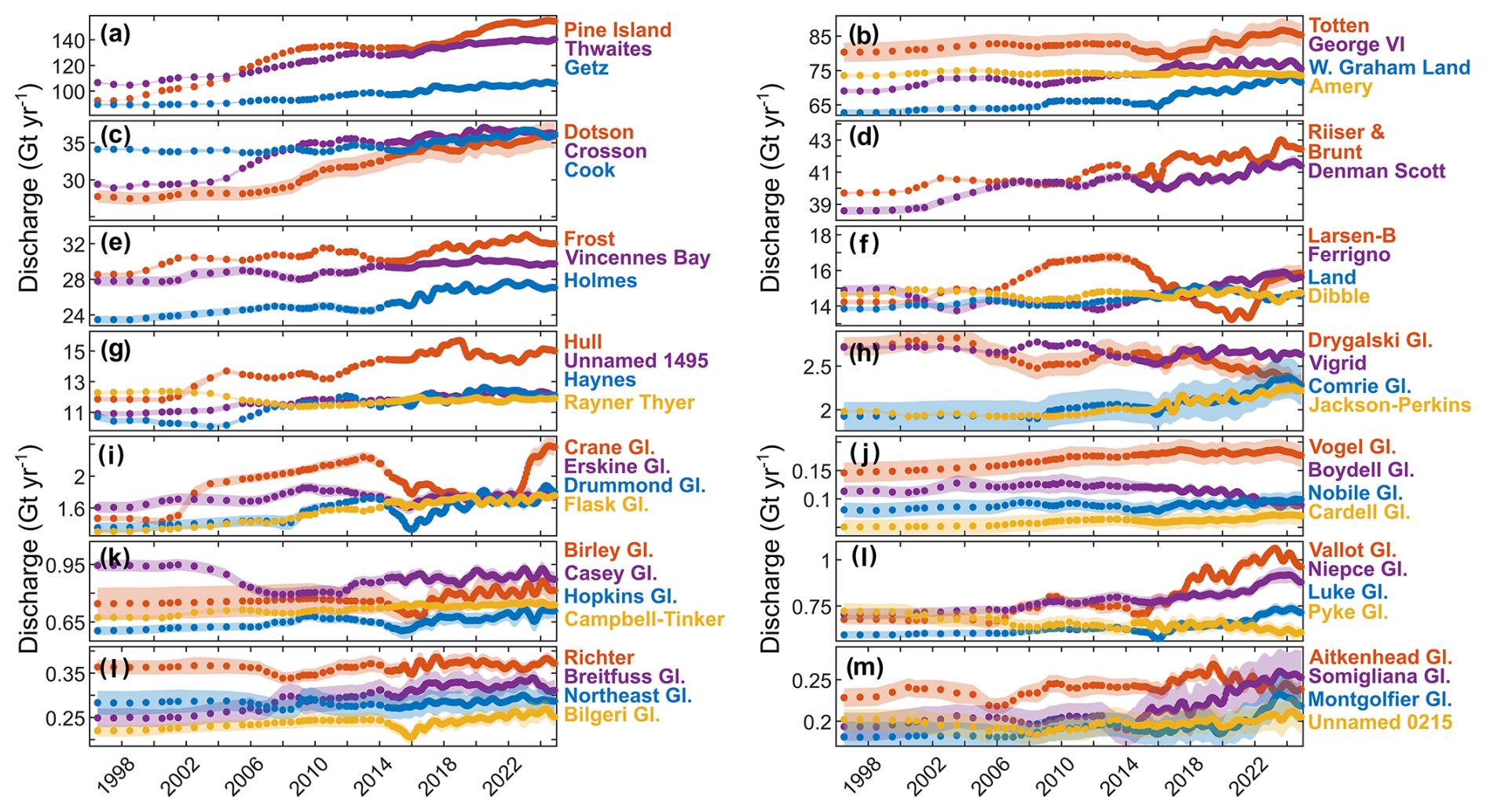
Figure 7 Basin-scale grounding line discharge examples. Grounding line discharge for selected basins from 1996 through 2024. The points show the gate-average discharge estimate, and the shading shows the discharge uncertainty (95 % confidence limits). Glacier locations are shown in Fig. 8.

Our dataset also provides grounding line discharge measurements for distinct Antarctic regions (Fig. 6). Grounding line discharge from West Antarctica increased from $\mathrm{793}\pm \mathrm{68}\mathrm{Gt}{\mathrm{yr}}^{-\mathrm{1}}$ in 1996 to $\mathrm{929}\pm \mathrm{80}\mathrm{Gt}{\mathrm{yr}}^{-\mathrm{1}}$ in 2024, with a trend of 5.3 Gt yr⁻² or 0.6 %yr⁻¹ and following a similar pattern of temporal variability described above. West Antarctica therefore currently accounts for approximately 42 % of all Antarctic grounding line discharge and 60 % of the total Antarctic increase in discharge from 1996 through 2024. Discharge from East Antarctica also increased from $\mathrm{945}\pm \mathrm{82}\mathrm{Gt}{\mathrm{yr}}^{-\mathrm{1}}$ in 1996 to $\mathrm{1001}\pm \mathrm{91}\mathrm{Gt}{\mathrm{yr}}^{-\mathrm{1}}$ in 2024, with a statistically significant trend of 2.2 Gt yr⁻². However, East Antarctic discharge is the most uncertain of any region and fluctuated on approximately 10-year timescales with an amplitude of approximately 20 Gt yr⁻¹. This relatively large uncertainty and temporal variability means that East Antarctic grounding line discharge during 2011–2015 was not significantly different from that during 2002–2008 and may explain previous reports of unchanging East Antarctic grounding line discharge that were based on comparisons between two epochs during those periods (Gardner et al., 2018). Grounding line discharge from the Antarctica Peninsula was $\mathrm{261}\pm \mathrm{25}\mathrm{Gt}{\mathrm{yr}}^{-\mathrm{1}}$ in 1996, increasing to $\mathrm{289}\pm \mathrm{29}\mathrm{Gt}{\mathrm{yr}}^{-\mathrm{1}}$ on average during April to September 2023, with a significant trend of 1.2 Gt yr⁻² or 0.4 %yr⁻¹. Our monthly discharge estimates since 2015 contain pronounced seasonal variations in discharge on the Antarctic Peninsula as a whole and on many of its outlet glaciers, as shown by two other studies to date (Boxall et al., 2022; Wallis et al., 2023). The seasonal cycles across the whole Peninsula have an amplitude of approximately 5–10 Gt yr⁻¹ but with substantial variability between years (Fig. 6).

Within the above regions, we provide discharge time series for individual glacier, ice stream and ice shelf basins. A selection of these basins, spanning discharges from less than 0.1 Gt yr⁻¹ to over 100 Gt yr⁻¹, are shown in Fig. 7. The top five contributors to Antarctic-wide grounding line discharge, on average since 2016, are Pine Island Glacier ($\mathrm{145}\pm \mathrm{3}\mathrm{Gt}{\mathrm{yr}}^{-\mathrm{1}}$), Thwaites Glacier ($\mathrm{136}\pm \mathrm{2}\mathrm{Gt}{\mathrm{yr}}^{-\mathrm{1}}$), Getz drainage basin ($\mathrm{103}\pm \mathrm{2}\mathrm{Gt}{\mathrm{yr}}^{-\mathrm{1}}$), Totten Glacier ($\mathrm{83}\pm \mathrm{0.3}\mathrm{Gt}{\mathrm{yr}}^{-\mathrm{1}}$) and George VI ($\mathrm{72}\pm \mathrm{1}\mathrm{Gt}{\mathrm{yr}}^{-\mathrm{1}}$). Discharge from Pine Island Glacier increased from 92±8 to $\mathrm{156}\pm \mathrm{13}\mathrm{Gt}{\mathrm{yr}}^{-\mathrm{1}}$ from 1996–2024, but this increase was interrupted by slightly declining discharge from 2009–2016, followed by steady discharge in 2021 and 2022 and a further increase in discharge since 2022 (Fig. 7a). Our dataset also includes other documented changes in grounding line discharge around Antarctica, including increases at Thwaites Glacier (Fig. 7a; Mouginot et al., 2014) and Crosson and Dotson ice shelves (Fig. 7c; Scheuchl et al., 2016) and a progressive deceleration of the Larsen B tributary glaciers until their recent acceleration in 2022 (Fig. 7f; Ochwat et al., 2023; Surawy-Stepney et al., 2023) and Whillans Ice Stream (Fig. 8; Joughin et al., 2005). Our dataset also reveals substantial changes in discharge at many glaciers and ice shelves that are less well known. These include, for example, increases in discharge from Cook Ice Shelf basin (Miles et al., 2022), Muller Ice Shelf, Denman Scott Glacier, Holmes, Vincennes Bay (primarily from Vanderford Glacier), Frost Ice Shelf and Ferrigno Ice Shelf, as well as numerous glaciers on the Antarctic Peninsula (Fig. 7). Other basins, such as Boydell Glacier, Drygalski Glacier and Pyke Glacier show declining discharge, whilst many others, such as Totten Glacier, undergo large multi-year fluctuations in discharge (Fig. 7).

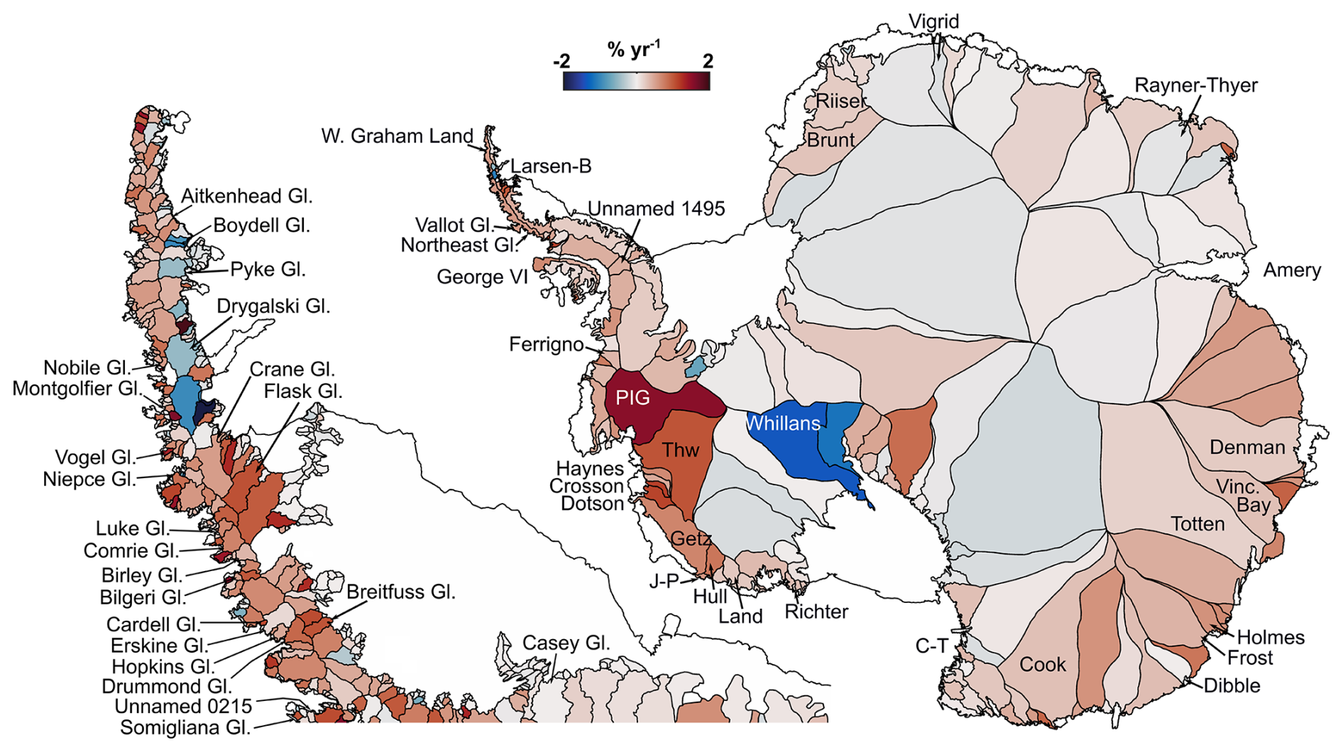
Figure 8 Basin-scale grounding line discharge trends from 1996–2024. Overview of grounding line discharge trends from 1996 through 2024 as a percentage of the median discharge in each drainage basin. Basins mentioned in the main text and Fig. 7 are labelled. Some basin names have been shortened for display purposes: Vinc. Bay is Vincennes Bay, PIG is Pine Island Glacier, Thw is Thwaites, Riiser is Riiser–Larsen, C-T is Campbell–Tinker, and J-P is Jackson–Perkins. The Antarctic Peninsula basins are from Cook et al. (2014), and the ice sheet basins are from Mouginot et al. (2017c).

Figure 8 provides an overview of 1996–2024 trends in grounding line discharge from individual glacier and ice stream basins around Antarctica. This overview highlights the rapid increase in grounding line discharge from the Amundsen Sea embayment of West Antarctica as well as weaker increases in the Bellingshausen Sea, the west coast of the Antarctica Peninsula and across the Indian Ocean-facing sector of Antarctica. It also shows declines in grounding line discharge from Whillans Ice Stream, numerous basins around Amery Ice Shelf in East Antarctica and many glaciers on the east coast of the Antarctic Peninsula (Fig. 8). This broad spatial pattern of grounding line discharge change is consistent with, but adds more detail to, changes in ice sheet surface elevation over a similar time period (Shepherd et al., 2019).

3.2 Effect of bed topography dataset on discharge

The choice of bed topography dataset affects the Antarctic-wide discharge estimate by 57 Gt yr⁻¹ on average (Fig. 9). BedMap2 gives discharge that is 4 % lower than BM + HF14 in West Antarctica, 1.4 % greater in East Antarctica and 24 % lower on the Antarctic Peninsula. The use of HF14 on the peninsula increases peninsula discharge by 21 % compared to using BedMachine only. Within individual MEaSUREs glacier basins, the discharge derived using BedMap2 is typically lower than from BM + HF14 by 1 % to 5 % (Fig. 9). The impact can be much larger for some individual basins, especially those on the Antarctic Peninsula; for example, the discharge from Drygalski Glacier is over 40 % lower using BedMap2 than it is with BM + HF14. The standard error in discharge across our 16 flux gates is similar between BM + HF14 and BedMap2 despite the increase in bed topographic observations and improvements in interpolation and assimilation methods since BedMap2 was developed.

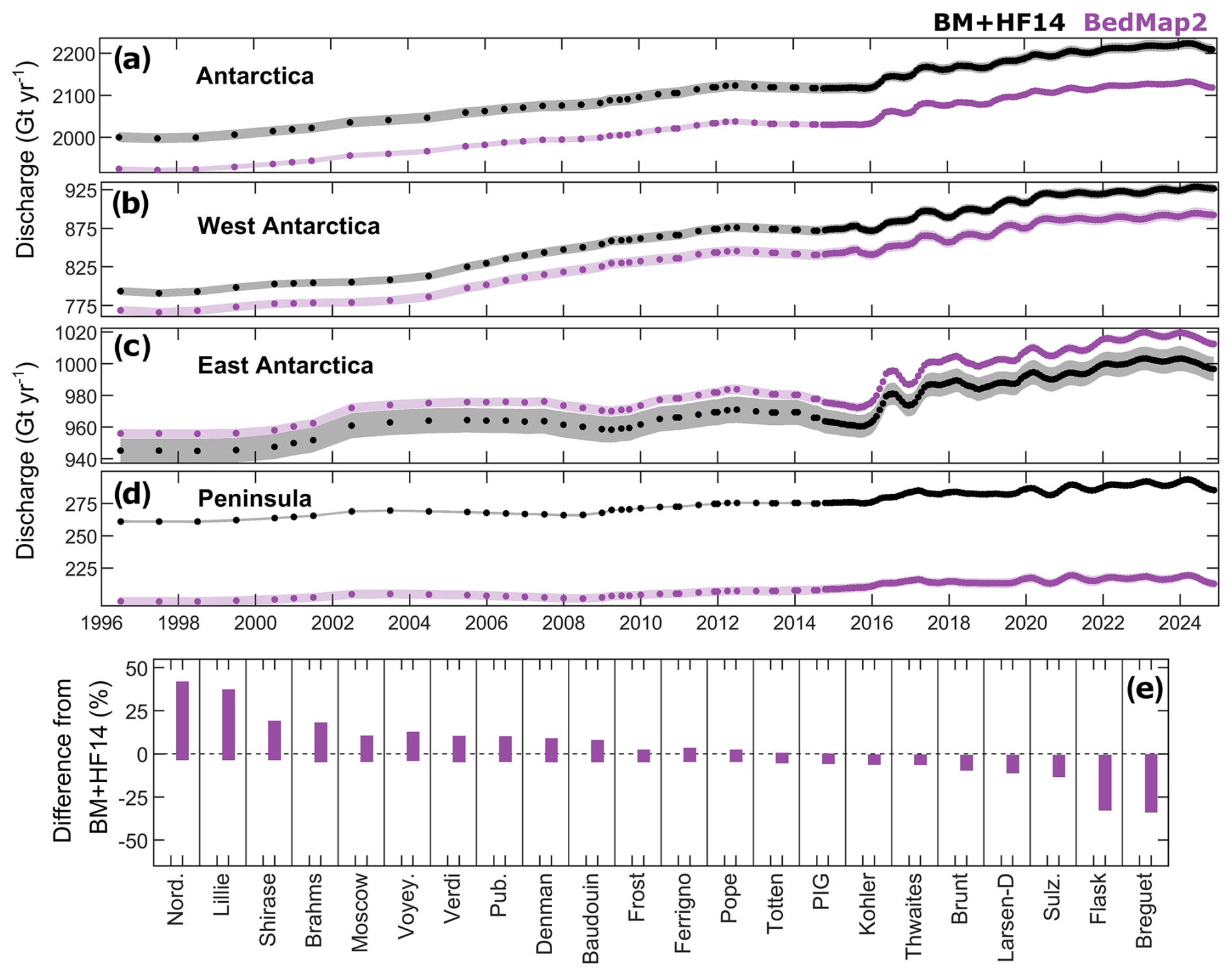
Figure 9 Impact of bed topography dataset on grounding line discharge. Grounding line discharge time series averaged across all flux gates for (a) Antarctica, (b) West Antarctica, (c) East Antarctica and (d) the Antarctic Peninsula. Panel (e) shows the percentage difference in grounding line discharge produced using BedMap2 compared to BM + HF14 for a range of drainage basins. The vertical extent of each bar represents the potential spread in the differences between bed products owing to error in each discharge estimate. Some basins have been shortened for display purposes: Nord. is Nordenskjold Ice Shelf, Voyey. is Voyeykov Ice Shelf, Pub. is Publications Ice Shelf, and Sulz. is Sulzberger Ice Shelf.

3.3 Effect of gate location

Antarctic-wide grounding line discharge varies by 48 Gt yr⁻¹ (2.2 %) on average between our most upstream and downstream flux gates, and individual gates are generally less than 2 % different from the gate-average discharge (Fig. 10). East Antarctica has the largest relative change in discharge between flux gates: discharge from the most seaward gate is 3.6 % greater than the most upstream gate and 2.4 % from the gate-mean discharge. The Antarctic Peninsula exhibits some seasonality in the inter-gate discharge differences (Fig. 10), likely reflecting seasonal changes in velocity retrieval in summer and winter. The differences between flux gates primarily reflects the difficulty in conserving mass with imperfect ice thickness, velocity and surface mass balance data, rather than algorithmic errors. Reflective of this, the location of the flux gate makes a small difference for basins where the bed is well surveyed. For example, at Pine Island Glacier, the maximum discharge difference between any flux gate and the gate average is just 1.2 Gt yr⁻¹ (0.9 %). Some studies (Gardner et al., 2018; Davison et al., 2023b) have minimised the impact of uncertain bed topography by placing their flux gates directly over bed topographic observations (primarily from radar flight lines). We opt instead to use the inverse error-weighted average of all gates, which has the advantage of permitting algorithmic gate generation and prioritises gates positioned closer to bed elevation observations since the error in the bed products is primarily determined by the distance to the nearest bed elevation observation.

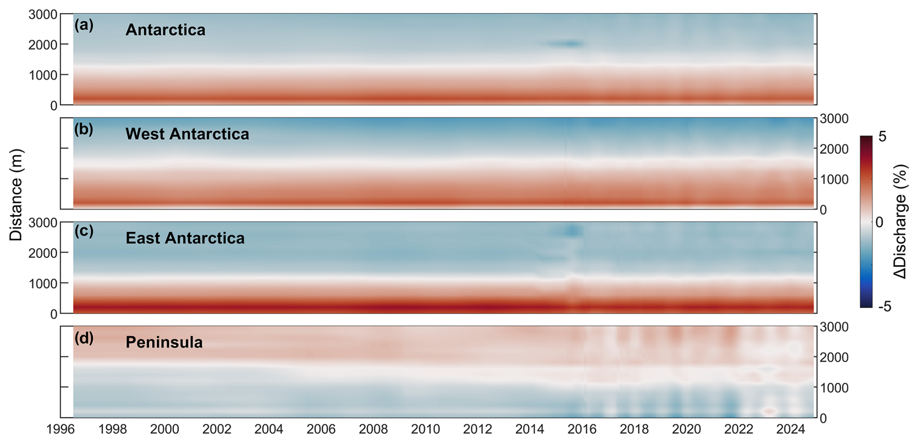
Figure 10 Impact of flux gate location on grounding line discharge. Time series of the percentage difference in grounding line discharge from the inverse error-weighted mean discharge across all flux gates for (a) Antarctica, (b) West Antarctica, (c) East Antarctica and (d) the Antarctic Peninsula. The y axes correspond to the distance upstream of the first flux gate.

3.4 Effect of thickness adjustments

We apply two modifications to the reference ice thickness extracted at each flux gate. These are (1) applying observed rates of surface elevation change based on a quadratic fit to elevation change observations from 1992–2023 to obtain a time series of ice thickness at each flux gate pixel and (2) removing firn air content using a time series of firn air content from two firn models. We also correct the basin-integrated discharge to account for surface mass balance changes between each flux gate and the grounding line. Antarctic-wide, the overall impact of these modifications is to increase grounding line discharge by 27 Gt yr⁻¹ in 1996 and reduce it by 7.7 Gt yr⁻¹ in 2024 (Fig. 11). The individual corrections for firn air content and surface mass balance impacts are larger (over 50 Gt yr⁻¹) but are opposing and change little over time. The majority of the change in the impact of these modifications from 1996 through 2024 is due to changes in ice surface elevation during that period, which cause an overall decrease in discharge of 28 Gt yr⁻¹ from 1996 through 2024 (Fig. 11). The impact of surface elevation changes on grounding line discharge is the greatest in West Antarctica where thinning rates are the highest (Figs. 11 and A1). The impact of firn air content removal is comparable in East and West Antarctica (approximately 21 Gt yr⁻¹ or 2 % discharge reductions each on average) and is the greatest in relative terms on the peninsula (12 Gt yr⁻¹ or 4 %). The effect of gate-to-grounding line SMB changes is to increase Antarctic grounding line discharge by 21 Gt yr⁻¹ at the most seaward flux gate, increasing to 105 Gt yr⁻¹ at the most upstream gate (Fig. 11).

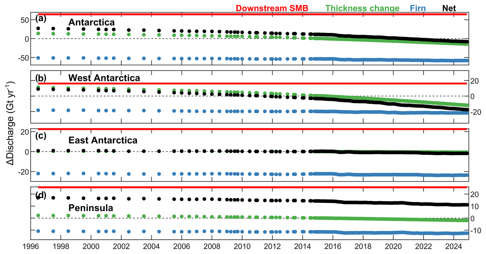
Figure 11 Time series of ice thickness and surface mass balance (SMB) corrections. The impact of SMB changes downstream of the flux gate (red dots), altimetry-derived thickness change (green dots) and removal of firn air content (blue dots) (described in text) on the derived grounding line discharge from (a) Antarctica, (b) West Antarctica, (c) East Antarctica and (d) the Antarctic Peninsula. The sum of the three corrections is also shown (black dots). Note that surface elevation changes are applied to our reference Antarctic Ice Sheet surface, which is timestamped to 9 May 2015.

The choice of firn densification model has a negligible (0.35 %) impact on Antarctic-wide grounding line discharge (Fig. 12) regardless of which flux gate is used. The IMAU-FDM gives consistently lower firn air content (Fig. 2d) so produces slightly higher discharge values than the GSFC-FDMv1.2. The differences between the firn models are generally the greatest (∼1 % discharge equivalent) on the peninsula, which we interpret to be primarily due to the ability of each model to resolve the impact of steep topography on surface processes, owing to their different spatial resolutions (12.5 km×12.5 km for the GSFC-FDMv1.2 and 27 km×27 km for the IMAU FDM). In some basins, the choice of firn model makes an appreciable difference; for example, at Moser Glacier, the IMAU-FDM decreases grounding line discharge by 4 % relative to the GSFC-FDMv1.2 on average. Basins with large relative differences are generally very small – with widths much smaller than the resolution of either firn model – so contribute little to total Antarctic discharge and require extraction from a single firn model pixel that will in many cases not resolve the glacier geometry. Overall, the use of a firn model has a large enough of an impact on grounding line discharge to be relevant to glacier mass balance, but the choice of firn model seems to have little impact on Antarctic discharge, at least for the two firn models examined here.

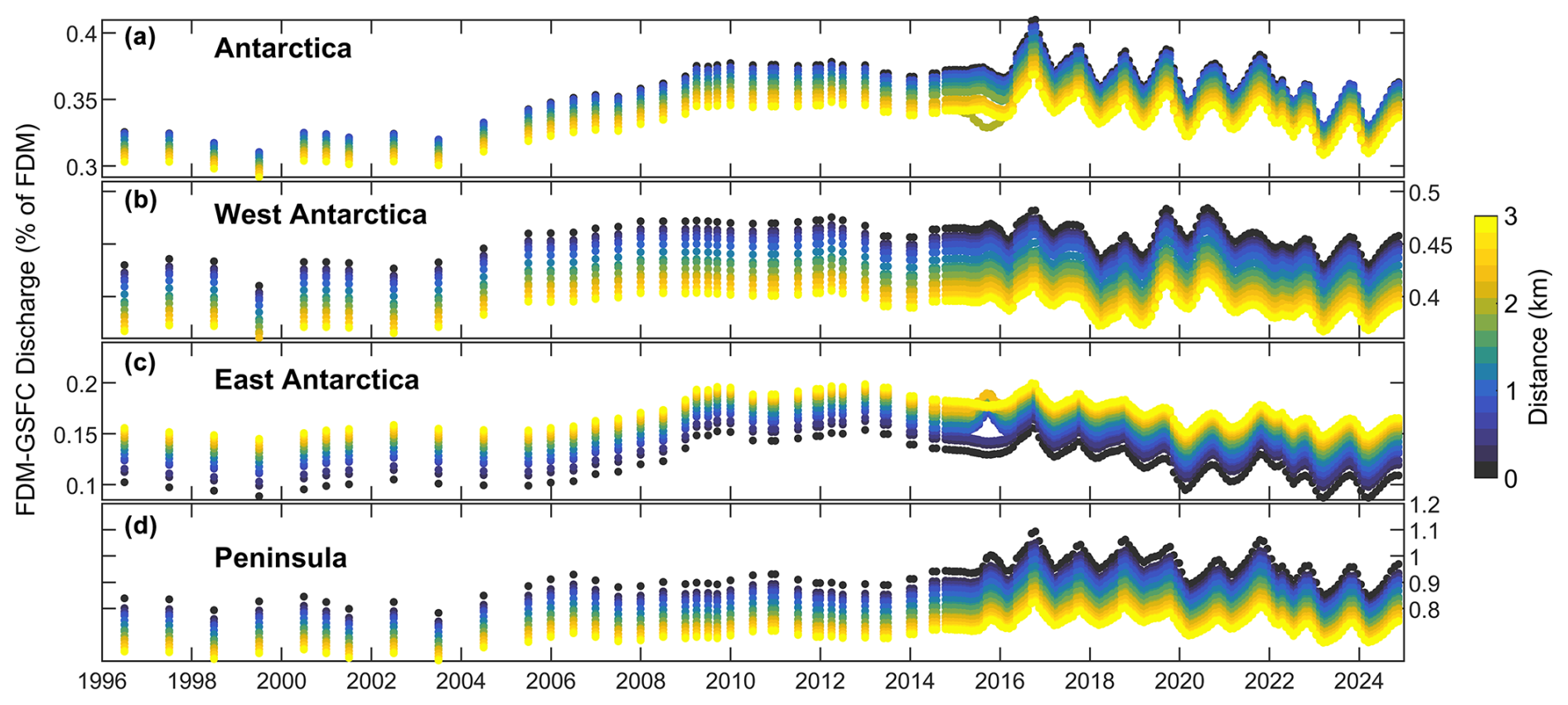
Figure 12 Impact of firn model choice on Antarctic grounding line discharge. Time series of the difference in grounding line discharge when using the IMAU FDM compared to the GSFC-FDMv1.2 from (a) Antarctica, (b) West Antarctica, (c) East Antarctica and (d) the Antarctica Peninsula. Points are coloured according to their distance in kilometres from the most downstream flux gate (blue) compared to the most inland flux gate (yellow).

4 Discussion

4.1 Comparison to previous estimates

We focus our comparison on previous estimates that encompass the majority or all of the Antarctic Ice Sheet (Gardner et al., 2018; Rignot et al., 2019; Depoorter et al., 2013; Miles et al., 2022). Miles et al. (2022) provide only percentage discharge changes, which hinders comparisons here, so we focus on the other datasets. For ease, we refer to Rignot et al. (2019) as R19, Depoorter et al. (2013) as D13 and Gardner et al. (2018) as G18. We note that the “2008” discharge estimates from G18 and D13 were estimated using a velocity mosaic (Rignot et al., 2017) compiled from images acquired during the 1996–2009 period, but the majority of those images were acquired between 2007 and 2009. To compare our discharge time series to those data, we use our average discharge from January 2007 to December 2009. Similarly, to enable comparisons with R19 we use the time-average discharge from both datasets during their overlapping time periods and common basins.

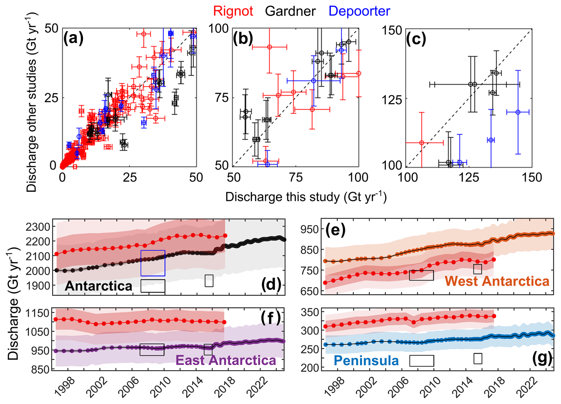
Figure 13 Comparison to existing grounding line discharge estimates. Panels (a)–(c) show comparisons with Rignot et al. (2019), Gardner et al. (2018) and Depoorter et al. (2013) for equivalent basins and during overlapping time periods. Each point shows the discharge for a single basin, with errors provided where available. Panels (d)–(g) show time series of our primary discharge estimate (using BM + HF14) compared to other estimates; data from Rignot et al. (2019) are shown as red dots, with dark shading indicating 5 % uncertainty and pale shading indicating 10 % uncertainty. The black boxes in panels (d)–(g) show data from Gardner et al. (2018), and the blue box in panel (d) shows data from Depoorter et al. (2013).

There are substantial differences between the few existing grounding line discharge estimates, and our results generally fall within the spread of existing estimates (Fig. 13). The common period for all datasets is 2007–2009, for which we estimate an Antarctic grounding line discharge of $\mathrm{2082}\pm \mathrm{178}\mathrm{Gt}{\mathrm{yr}}^{-\mathrm{1}}$, whilst the other studies estimate $\mathrm{2190}\pm \mathrm{142}\mathrm{Gt}{\mathrm{yr}}^{-\mathrm{1}}$ (R19), $\mathrm{1894}\pm \mathrm{43}\mathrm{Gt}{\mathrm{yr}}^{-\mathrm{1}}$ (G18) and $\mathrm{2049}\pm \mathrm{87}\mathrm{Gt}{\mathrm{yr}}^{-\mathrm{1}}$ (D13). The overall spread of all four estimates is 296 Gtyr⁻¹ or 14.4 % relative to the mean, from which our estimate differs by 28 Gt yr⁻¹ or 1.4 % of the mean. For West Antarctica, our 2007–2009 discharge estimate of $\mathrm{853}\pm \mathrm{71}\mathrm{Gt}{\mathrm{yr}}^{-\mathrm{1}}$ is approximately 100 Gt yr⁻¹ greater than R19 ($\mathrm{749}\pm \mathrm{42}\mathrm{Gt}{\mathrm{yr}}^{-\mathrm{1}}$) and G18 ($\mathrm{724}\pm \mathrm{24}\mathrm{Gt}{\mathrm{yr}}^{-\mathrm{1}}$). For East Antarctica, our 2007–2009 estimate of $\mathrm{960}\pm \mathrm{82}\mathrm{Gt}{\mathrm{yr}}^{-\mathrm{1}}$ is very similar to the $\mathrm{952}\pm \mathrm{31}\mathrm{Gt}{\mathrm{yr}}^{-\mathrm{1}}$ from G18, both of which are $\sim \mathrm{50}\mathrm{Gt}{\mathrm{yr}}^{-\mathrm{1}}$ lower than the $\mathrm{1111}\pm \mathrm{69}\mathrm{Gt}{\mathrm{yr}}^{-\mathrm{1}}$ from R19. Our discharge estimate of $\mathrm{268}\pm \mathrm{25}\mathrm{Gt}{\mathrm{yr}}^{-\mathrm{1}}$ from the Antarctic Peninsula falls between existing estimates, which range from $\mathrm{217}\pm \mathrm{15}\mathrm{Gt}{\mathrm{yr}}^{-\mathrm{1}}$ (G18) and $\mathrm{330}\pm \mathrm{26}\mathrm{Gt}{\mathrm{yr}}^{-\mathrm{1}}$ (R19). D13 did not provide estimates for East Antarctica, West Antarctica or the peninsula. Overall, our Antarctica discharge estimate agrees with D13 and falls between R19 and G18. In West Antarctica, our estimates are consistently greater than G18 and R19 but overlap within error with R19. In East Antarctica, our estimates agree with D18 but are consistently lower than R19. On the peninsula, our estimate falls between that of R19 and G18.

At smaller scales, there are differences between the available discharge estimates within individual basins (Fig. 14 and Table S1 in the Supplement). In East Antarctica, our grounding line discharge is typically lower in each of the MEaSUREs glacier basins, though Totten is the obvious exception to this pattern. In West Antarctica, our grounding line discharge from the MEaSUREs glacier basins are typically larger than R19. For the major basins in the Amundsen Sea embayment, our estimates are similar to other estimates. For example, our Pine Island discharge differs from R19 by just 5 Gt yr⁻¹ on average (although it is almost always greater in this study) and at most by 15 Gt yr⁻¹ in 2008, which is reflected in the 17 Gt yr⁻¹ difference to D13 at Pine Island. At Thwaites Glacier, the differences are 12 Gt yr⁻¹ compared to R19 and 19 Gt yr⁻¹ for D13. G18 provide discharge for basin 22 (approximately Pine Island and Thwaites combined), which agrees with our estimates to within 2 Gt yr⁻¹ in 2008 and 6 Gt yr⁻¹ in 2015. Several basins have very large (>50 %) percentage residuals compared to R19, for example, Kamb Ice Stream, but these basins all have very low discharge ($<\mathrm{1}\mathrm{Gt}{\mathrm{yr}}^{-\mathrm{1}}$).

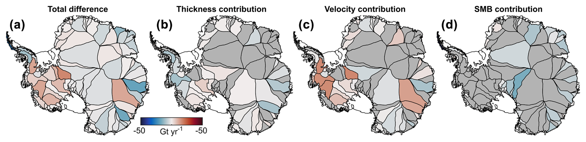
Figure 14 Contributions to differences with Rignot et al. (2019) in each MEaSUREs glacier basin. (a) Time-average difference between this study and Rignot et al. (2019), during overlapping time periods. (d) Contribution of ice thickness to the total discharge difference. (c) Contribution of everything except ice thickness, assumed to be predominantly due to ice velocity differences, to the total discharge difference. (d) Contribution of surface mass balance (SMB) uncertainty (from the spread in SMB estimates in three regional climate models) to the discharge difference, in basins where Rignot et al. (2019) used the long-term average SMB to estimate the balance ice flux.

The basin-scale contributions of ice thickness, ice velocity and SMB to the discharge differences between this study and R19 are shown in Fig. 14. We estimate the contributions of ice velocity and thickness to discharge differences as follows: for the MEaSUREs glacier basins in which R19 used BedMap2 as their thickness source, we assume the differences between our BedMap2-based discharge and R19 are entirely due to ice velocity differences. This is a simplification that will form an upper bound on the velocity contribution. Although we incorporate MEaSUREs annual velocity mosaics into our grounding line discharge estimate, differences owing to ice velocity are nevertheless expected because (1) we reduce offsets between velocity data sources using a temporal moving mean filter, whereas R19 use only the MEaSUREs annual mosaics and a reference velocity grid; (2) we fill gaps in our velocity estimates primarily using linear temporal interpolation, whereas R19 use linear spatial interpolation of velocity or the nearest in time ice velocity or flux estimate, depending on the size of the data gap; and (3) where velocity coverage is low, R19 scale their fluxes and velocities across the whole basin based on changes in speed in the fastest part of the basin when it is observed. For basins where R19 assume steady-state discharge, derived from the long-term average SMB from a combination of RACMO2.3p1 and p2, we cannot estimate the contributions of thickness and velocity of the discharge discrepancy. Instead, we estimate the SMB contribution to the discharge difference as the spread in SMB estimates among RACMO2.3p2, MAR and HIRHAM5.

For the major Amundsen Sea embayment basins, our use of BM + HF14 decreases ice discharge compared to BedMap2, but differences in ice velocity more than offset this, resulting in slightly greater discharge than R19 (Fig. 14). For the Ross West ice streams, both differences in ice thickness and ice velocity contribute approximately equally to the greater discharge we estimate there. In other basins (e.g. Academy, Aviator, Byrd, Larsen C, Mertz, Ninnis and Sulzberger), BM + HF14 increases discharge compared to BedMap2, whilst velocity differences decrease it, generally resulting in a small net decrease in discharge compared to R19.

Out of the 199 MEaSUREs glacier basins, our estimates agree within error with R19 at 170 basins (85 %), with a root mean square error between datasets of 17.5 Gt yr⁻¹. In 15 of the 29 remaining basins, R19 use steady-state discharge from modelled SMB. For 13 of those 15 basins, the SMB uncertainty (from the spread in SMB estimates from three RCMs) is greater than the difference between our discharge and R19. The remaining two basins where R19 used balance flux are Princess Martha Coast1 and Princess Astrid Coast1, which each discharge less than 0.05 Gt yr⁻¹ in R19. That leaves 14 basins where our estimates do not overlap with R19. The total difference between our discharge and R19 in those 14 basins is 69 Gt yr⁻¹, the majority of which (59 Gt yr⁻¹) stems from six basins (Whillans, MacAyeal, Foundation, Evans, Crosson and Bindschadler). With the exception of Whillans, differences in ice velocity overwhelmingly cause the discharge discrepancies from those basins.

4.2 Implications for mass budget estimates

At present, only one input–output estimate of Antarctic Ice Sheet mass balance is available (Rignot et al., 2019). This sparsity of input–output data limits the otherwise comprehensive scope of ice sheet mass balance intercomparison exercises (Otosaka et al., 2023) and limits insights conferred by mass budget partitioning attempts. Here, we examine the mass balance implied by our grounding line discharge and the mean of three regional climate models (Fig. 15) in comparison to a reconciled mass balance estimate (Otosaka et al., 2023). Using BM + HF14, we find that mass balance of Antarctica, West Antarctica, East Antarctica and the peninsula from 2017 through 2020 is $-\mathrm{90}\pm \mathrm{20}$, $-\mathrm{243}\pm \mathrm{7}$, 147±19 and $\mathrm{10}\pm \mathrm{6}\mathrm{Gt}{\mathrm{yr}}^{-\mathrm{1}}$, respectively. For comparison, the latest Ice Sheet Mass Balance Intercomparison Exercise (IMBIE) found mass change rates of $-\mathrm{115}\pm \mathrm{55}\mathrm{Gt}{\mathrm{yr}}^{-\mathrm{1}}$ (Antarctica), $-\mathrm{94}\pm \mathrm{25}\mathrm{Gt}{\mathrm{yr}}^{-\mathrm{1}}$ (West Antarctica), $\mathrm{0}\pm \mathrm{47}\mathrm{Gt}{\mathrm{yr}}^{-\mathrm{1}}$ (East Antarctica) and $\mathrm{21}\pm \mathrm{12}\mathrm{Gt}{\mathrm{yr}}^{-\mathrm{1}}$ (peninsula), respectively. Each of our mass balance estimates capture the interannual and longer-term variability in rate of mass change visible in the IMBIE dataset, but the magnitude and sign of mass change varies substantially between discharge estimates (Fig. 15). Our BM + HF14 mass balance generally overlaps with the uncertainty in IMBIE for Antarctica as a whole and at times on the peninsula but results in an >100 % greater rate of mass loss from West Antarctica compared to IMBIE and implies rapid (150 Gt yr⁻¹) mass gain in East Antarctica rather than negligible mass change. Figure 13 shows that the spread in discharge estimates from this study and other studies (Gardner et al., 2018; Rignot et al., 2019; Depoorter et al., 2013) is such that they have different implications for the direction of mass change in major regions of Antarctica. This has been demonstrated previously at the ice sheet scale (Mottram et al., 2021) and on the peninsula (Hansen et al., 2021). This discharge-induced uncertainty in input–output mass balance is compounded by the $\sim \mathrm{500}\mathrm{Gt}{\mathrm{yr}}^{-\mathrm{1}}$ spread in modelled SMB estimates, depending on which regional climate model is used (Mottram et al., 2021). The combined uncertainty in discharge and SMB must be narrowed to improve the accuracy of the input–output method for estimating Antarctic Ice Sheet mass change at any spatial and temporal scale. This is true also for other approaches to calculate ice sheet mass balance that rely on SMB data as an input.

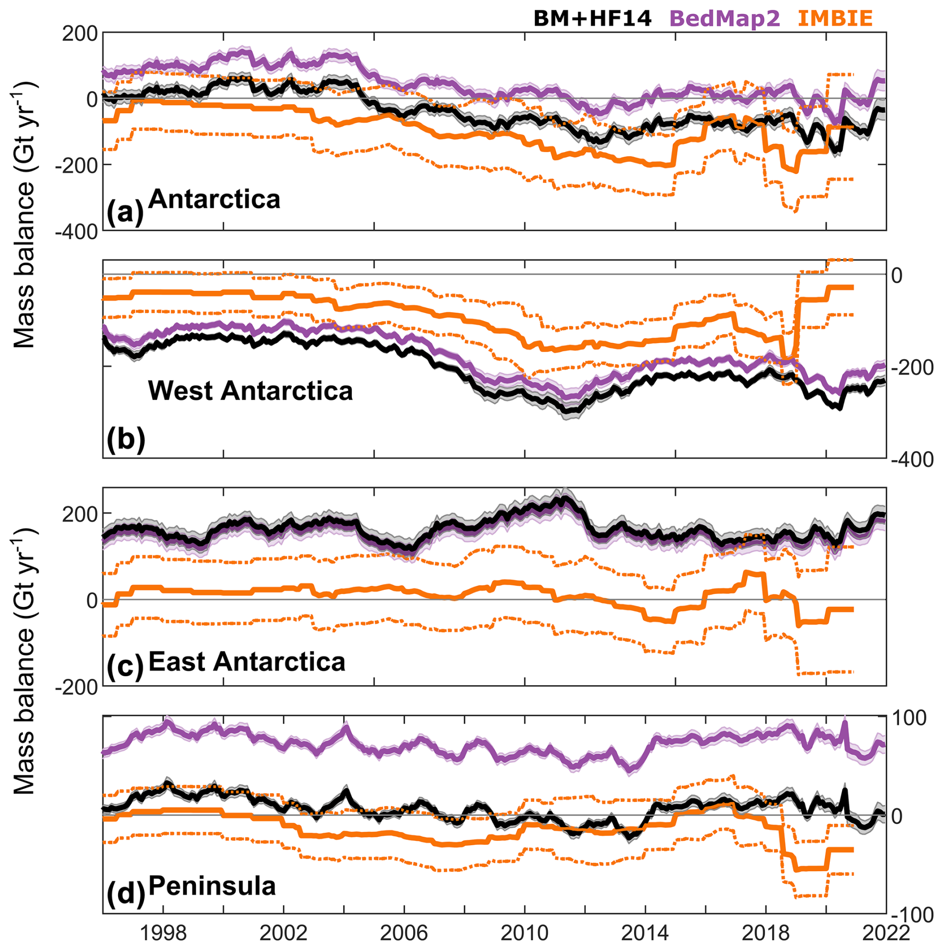
Figure 15 Antarctic Ice Sheet mass balance. Mass balance time series for (a) Antarctica, (b) West Antarctica, (c) East Antarctica and (d) the Antarctic Peninsula, compared to the third IMBIE assessment in orange (Otosaka et al., 2023). Mass balance is calculated using the mean of the three regional climate models described in the main text.

5 Data availability

The ice sheet basins, balance discharge and grounding line discharge estimates are available at https://doi.org/10.5281/zenodo.10051893 (Davison et al., 2024).

6 Conclusions

We present a new grounding line discharge product for Antarctica and all of its drainage basins available from 1996 through to November 2024. The temporal resolution and coverage increase from annual and <25 %, respectively, in the early years of our dataset to monthly and over 50 %, respectively, in the latter years of our dataset. We show that grounding line discharge from Antarctica increased from $\mathrm{1999}\pm \mathrm{175}\mathrm{Gt}{\mathrm{yr}}^{-\mathrm{1}}$ in 1996, rising to $\mathrm{2224}\pm \mathrm{200}\mathrm{Gt}{\mathrm{yr}}^{-\mathrm{1}}$ in 2024. Much of this grounding line discharge change is due to increasing flow speeds of West Antarctic ice streams, but we also observe large increases in discharge at some basins in East Antarctica, including Holmes, Vanderford Glacier, Denman Scott and Cook Ice Shelf. The high spatial and temporal resolution of our ice velocity mosaics since October 2014 allows us to measure substantial seasonal variability and pronounced multi-year trends in discharge even on small ∼1 km wide glaciers draining the Antarctic Peninsula.

There are large differences between existing Antarctic discharge estimates, and our estimates generally fall within this range. These differences arise primarily due to uncertainties in both bed topography and ice velocity, but the choice of flux gate location, velocity gap filling approaches and other algorithm choices also contribute. For some basins, the differences between existing discharge datasets, including our own, are significant enough to have bearing on the mass change of those basins when using the input–output method, particularly in basins which remain close to balance but which are persistently above or below balance. This is particularly acute on the Antarctic Peninsula and in East Antarctica, where deriving estimates of ice thickness, ice velocity, firn air content and surface mass balance is fraught with difficulties owing to the steep topography, narrow glaciers, high snowfall and (in places) intense summertime surface melting.

We emphasise that significant uncertainty in both grounding line discharge and SMB currently limits the utility of the input–output method for estimating ice sheet mass change, therefore further work must be done to address this. These uncertainties need to be narrowed to support multi-method mass balance assessments and to improve estimates of the dynamic and SMB contributions to mass change, which inform our understanding of the spatially and temporally varying drivers of ice sheet mass change. The progressive increase in ice thickness measurements around Antarctica (Frémand et al., 2023) and the improvements in assimilation and interpolation methods (Morlighem et al., 2020; Leong and Horgan, 2020) will lead to improved estimates of ice thickness around Antarctica; our workflow is designed to facilitate the addition of new bed topography datasets as they become available, and we aim to do so. However, we suggest that more validation of modelled SMB and ice velocity is also required to accurately estimate Antarctic mass balance using the input–output method. Irrespective of the implications for mass balance, grounding line discharge remains an important metric for measuring and investigating ice dynamic change; our dataset reveals substantial variability in discharge at hundreds of individual glaciers, offering huge opportunity for furthering our understanding into environmental and internal drivers of flow variability.

Appendix A: Sentinel-1 ice velocity maps

We generate monthly velocity mosaics from October 2014 through to January 2024 by applying standard intensity tracking techniques (Strozzi et al., 2002) to Copernicus Sentinel-1 synthetic aperture radar (SAR) single look complex (SLC) interferometric wide (IW) mode image pairs (Hogg et al., 2017; Davison et al., 2023b). We process all available 6 and 12 d image pairs acquired over Antarctica; all image pairs prior to the launch of Sentinel-1b in April 2016 and after the failure of Sentinel-1b in December 2021 are 12 d pairs. We estimate ice motion by performing a normalised cross-correlation between image patches with dimensions of 256 pixels in range and 64 pixels in azimuth and a step size of 64 pixels in range and 16 pixels in azimuth. To maximise tracking results in regions where velocity varies by more than an order of magnitude, we also use patch sizes of 362×144 and 400×160 pixels over East and West Antarctica and 4 further patch sizes on the Antarctic Peninsula (192×48, 224×56, 288×72 and 320×80 pixels in range and azimuth). For scenes in East and West Antarctica, we use the 1 km DEM (Bamber et al., 2009), whereas for scenes in the Antarctic Peninsula, we use the REMA 200 m DEM (Howat et al., 2019). Prior to image cross-correlation, we perform image geocoding using the precise orbit ephemeris (accurate to 5 cm) where available and the restituted orbits otherwise (accurate to 10 cm) (Fernández et al., 2015). In common with comparable estimates of Greenland Ice Sheet velocity (Solgaard et al., 2021), we find no significant difference between pairs processed using each orbit type. Each image pair velocity field is posted on a 100 m×100 m grid in Antarctic polar stereographic coordinates (EPSG 3031).

For each image pair, we generate a signal-to-noise ratio (SNR) weighted mean velocity field of all available cross-correlation window sizes after removing outliers in the 2-D velocity fields. To remove outliers in each window size for every scene pair, we first compare each speed field to a reference speed map (Rignot et al., 2017); speed estimates more than 4 times greater or 4 times smaller than the reference map are considered outliers and removed. Secondly, flow directions more than 45° different from the reference map are considered outliers and removed. Thirdly, pixels in which the speed differs by more than 3 standard deviations from its neighbours in a 5×5 moving window are removed. Similarly, pixels in which the flow direction differs by more than 45° from its neighbours in a 5×5 moving window are removed. Finally, we use a hybrid median filter with a 3×3 moving window which removes the central pixel if it more than 3 times the median of the horizontally and diagonally connected pixels. After forming the SNR weighted mean of the resulting velocity fields, we generate Antarctic-wide mosaics of ice velocity for every unique date pair since October 2014. From these date-pair mosaics, we generate monthly Antarctic-wide velocity mosaics as the mean of all date pairs that overlap with the target month. When doing so, we weight each date pair by the number of days of overlap with the target month; in this way, 12 d pairs are weighted twice as much as 6 d pairs, which is appropriate because they should contribute more to the average velocity in the month. We also generate two quality parameters, the number of observations in each month in each pixel (after outlier removal) and the proportion of each month that is observed in each pixel in addition to an error estimate defined as the speed divided by the SNR (Lemos et al., 2018).

Appendix B: Ice velocity data source differences and alignment

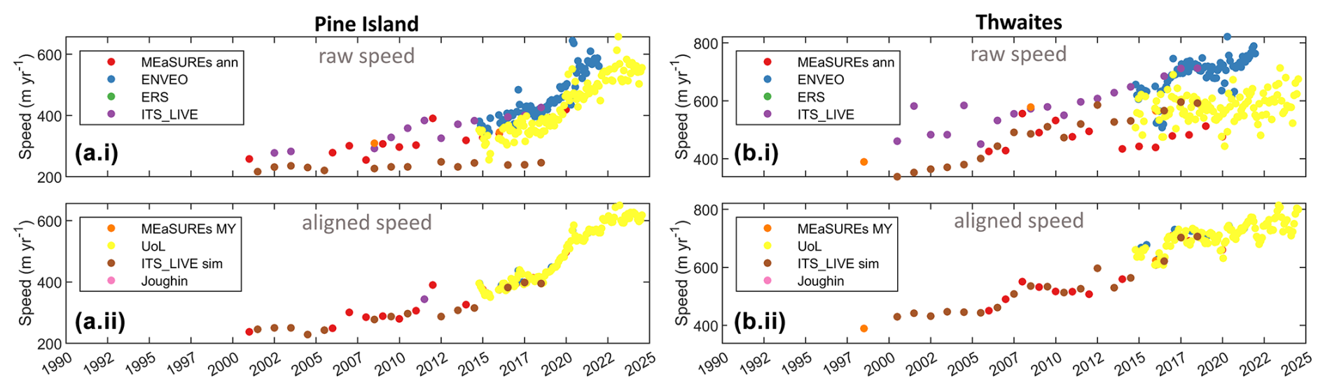
Figure B1 Velocity alignment example one. Panels (a.i) and (b.i) show the raw speed from a single pixel on our most seaward flux gate. Panels (a.ii) and (b.ii) show the final aligned speed.

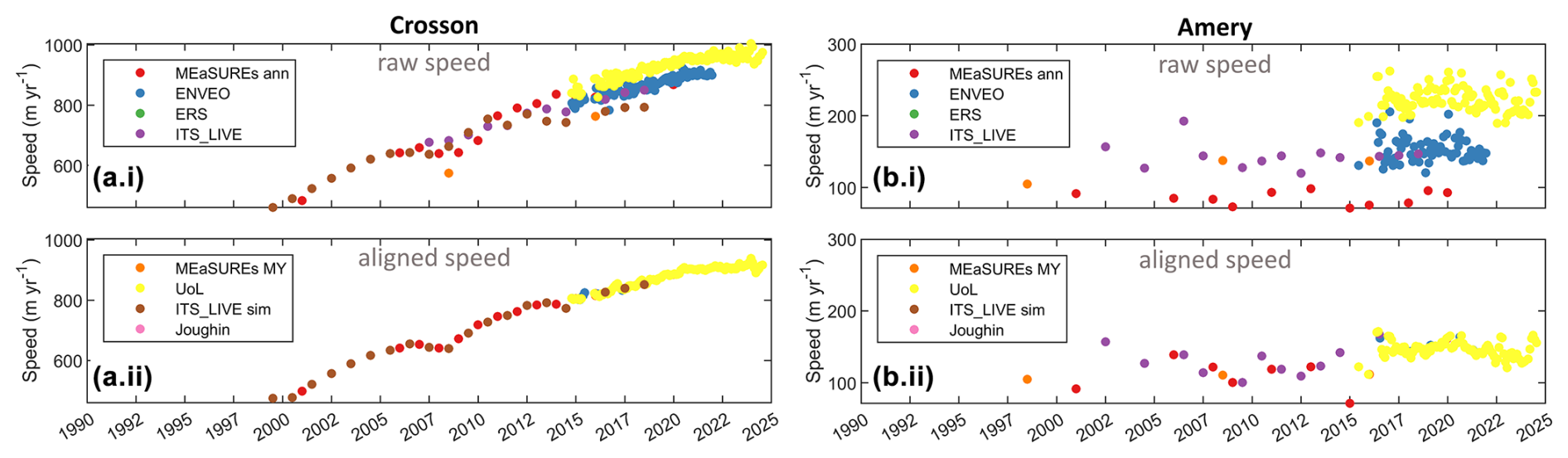
Figure B2 Velocity alignment example two. Panels (a.i) and (b.i) show the raw speed from a single pixel on our most seaward flux gate. Panels (a.ii) and (b.ii) show the final aligned speed.

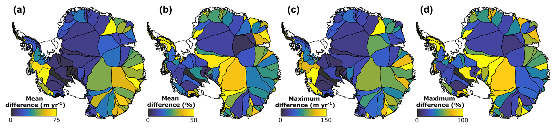
Figure B3 Velocity alignment overview. Each panel shows the differences between all velocity data sources in all flux gate pixels in each MEaSUREs glacier basin. The individual data sources are as described in the main text. Differences between velocity data sources are calculated in 1-year moving windows prior to alignment and averaged through time in each flux gate pixel prior to calculating basin-scale statistics. (a) The mean velocity difference, in metres per year. (b) The mean difference as a percentage of the basin- and time-averaged post-aligned speed. (c) The maximum time-averaged difference. (d) As for panel (c) as a percentage of the basin- and time-averaged post-aligned speed.

We use eight sources of velocity data to estimate grounding line discharge. These velocity datasets span different spatial extents and time periods. Where they overlap in space and time, there are differences between velocity estimates from different data sources. Generally, the differences in velocity between data sources are systematic in a given location; for example, one data source will be consistently slower or faster than another data source. These differences can arise for several reasons. Firstly, the differences could reflect true temporal variations in ice velocity when, for example, comparing annual averages centred on June (ITS_LIVE) vs. December (MEaSUREs). Secondly, differences can arise particularly in shear margins due to different feature tracking choices, including (but not limited to) window and step sizes, image co-registration algorithms, image pre-processing to enhance feature visibility, and cross-correlation peak-finding algorithms.

Figures B1 and B2 shows examples of such differences and the resulting aligned speed from single pixels along our most seaward flux gate. The differences between data sources at a given time are typically 50–100 m yr⁻¹ but can be several hundred metres per year. Figure B3 shows the average and maximum differences between data sources in each of the MEaSUREs glacier basins.

To reduce the differences between data sources, we make the assumptions that no single velocity dataset is perfect and that all velocity datasets will be clustered around the true velocity. We therefore use a simple moving-mean filter to align the data sources. We first use the difference between the median of the linear fits through the ENVEO and University of Leeds datasets during their overlapping time periods to shift the University of Leeds data over the ENVEO data. This first step is necessary because the University of Leeds data extend beyond the temporal extent of any other dataset. We then use a moving-mean filter with a five-point window size on all data sources except the University of Leeds and ENVEO (both of which provide monthly velocities). We then use a 3-month moving mean filter to align the monthly datasets and further align the other datasets.

It is not possible to determine exactly what impact this alignment has on the grounding line discharge estimate. Using no alignment results in much greater data loss during the outlier removal stages and a much more variable discharge when the underlying velocity data source changes. Using larger moving-mean window sizes has the effect of smoothing the discharge time series but does not greatly affect the average discharge. Using smaller window sizes can result in some data sources being unaligned, especially when coverage is low, again resulting in more variable discharge.