A high-resolution temperature–salinity dataset observed by autonomous underwater vehicles for the evolution of mesoscale eddies and associated submesoscale processes in the South China Sea

Marginal seas are often characterized by dynamic mesoscale eddies (MEs), whose evolution plays a critical role in regulating global oceanic energy budgets, triggering submesoscale processes with strong vertical velocity, and facilitating biogeochemical transport. However, traditional observation methods, constrained by passive sampling modes, struggle to resolve the temporal evolution of MEs and associated submesoscale processes at kilometer-scale resolutions. Autonomous underwater vehicles (AUVs) and underwater gliders (UGs), operating in active sampling modes, provide spatio-temporal synchronized measurements of these highly dynamic features. Here, we present a 9-year (2014–2022) high-resolution temperature–salinity dataset collected by AUVs/UGs in the South China Sea (SCS), accessible via https://doi.org/10.57760/sciencedb.11996 (Qiu et al., 2024b). In total, the dataset comprises 11 cruise experiments that deployed 50 UGs and two AUVs, achieving spatial and temporal resolutions of < 7 km and < 7 h, respectively. This dataset offers unprecedented insights into ME evolution life stages, covering the zones of an eddy's birth, propagation, and dissipation. A total of 40 % of the data resolve submesoscale processes (< 1 km, < 4 h), capturing dynamic instabilities along and across frontal zones at eddy peripheries. This dataset has the potential to improve the forecast accuracy in physical and biogeochemistry numerical models. Much more aggressive field investigation programs will be promoted by the National Natural Science Foundation of China in the future.

1 Introduction

The evolution of mesoscale eddies (MEs), characterized by intense geostrophic strain rates, leads to the generation of submesoscale processes with kilometer-scale spatial resolutions (McWilliams, 2016). This dynamic interplay requires observational systems with high spatio-temporal synchronization and enhanced resolution capabilities. MEs obtain kinetic energy from large-scale currents and subsequently dissipate to submesoscale or finer-scale processes in the slope regions via combined shear and baroclinic instabilities (Oey, 1995; Okkonen et al., 2003). Marginal seas (such as the Gulf of Mexico or the Mediterranean Sea) are usually filled with MEs (Rossby number $R_{\mathrm{o}}=U/fL\approx \mathrm{0.1}$), alongside smaller-scale processes (R_o>1). The South China Sea (SCS), as a tropical marginal sea, demonstrates particularly vigorous ME dynamics (Chen et al., 2011; Wang et al., 2003; Xiu et al., 2010). These coherent vortices, spanning 50–300 km horizontally and persisting several weeks to months, play vital roles in the transport of matter and energy (Chelton et al., 2007; Morrow et al., 2004).

Table 1 Previous observational studies of mesoscale eddies (MEs) in the South China Sea.

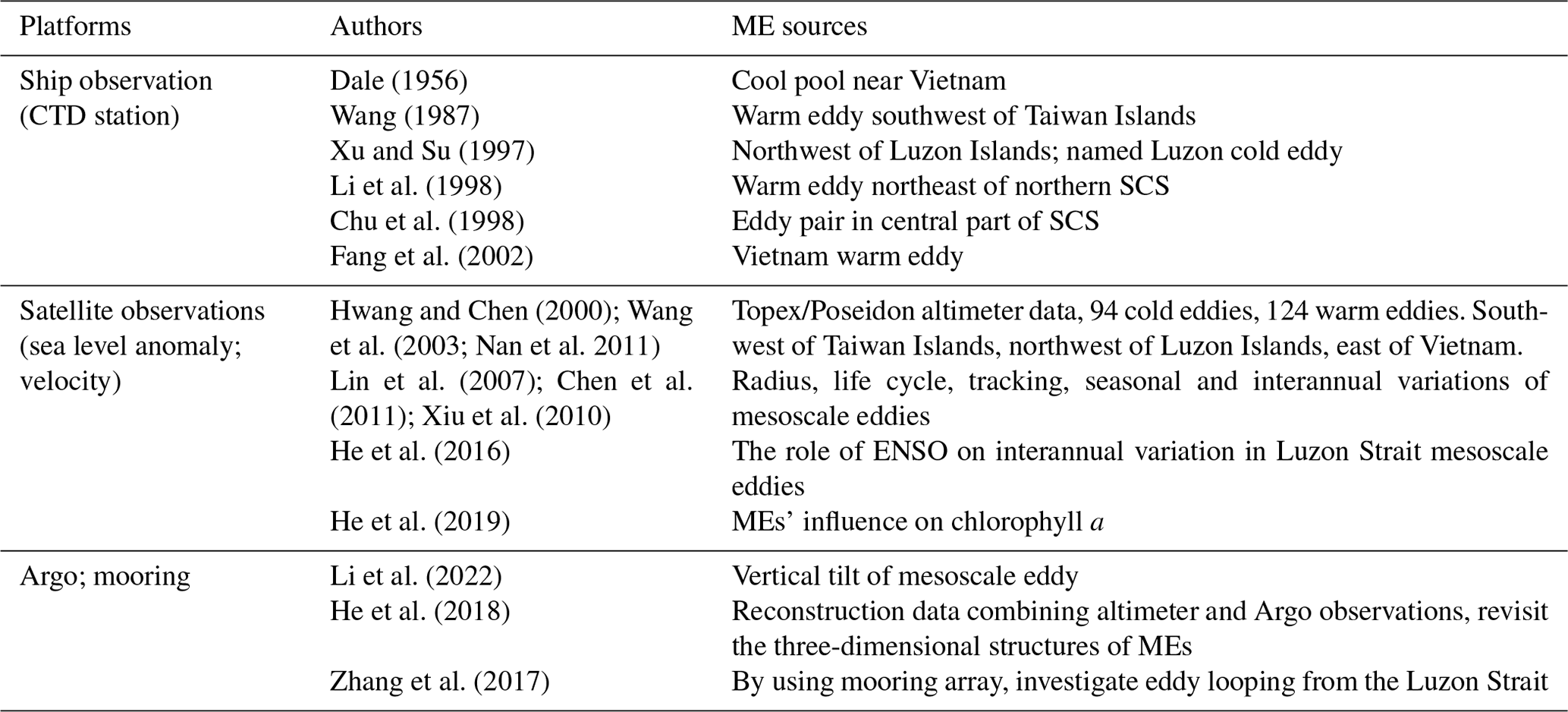
Contemporary observation platforms for MEs include shipborne surveys, satellite remote sensing, Argo float arrays, Lagrangian drifters, autonomous underwater vehicles (AUVs), and underwater gliders (UGs). While ship-based observations are the most fundamental to investigate MEs' general structures, their temporal resolution limits continuous evolution tracking. Satellite altimetry provides comprehensive surface signatures of MEs, including spatio-temporal metrics, radius evolution, and trajectory mapping (Chelton et al., 2011). Four primary ME generation hotspots have been identified in the SCS: southwest of Taiwan, northwest of the Luzon Islands, the Xisha Islands region, and the eastern Vietnamese coastal zone (Hwang and Chen, 2000; Wang et al., 2003; Nan et al., 2011). ME propagation patterns (westward, southwestward, or northwestward) are predominantly governed by first-baroclinic Rossby wave dynamics (Lin et al., 2007; Xiu et al., 2010; Chen et al., 2011). Since 2002, a large number of Argo arrays have been deployed, providing routine measurements to describe the vertical structures of MEs (He et al., 2018; Table 1). However, the spatio-temporal resolutions of Argo profiles are approximately 100 km and 10 d, remaining insufficient to capture the high-frequency variability of MEs and submesoscale processes (Table 1).

Attributed to the active tracking, AUVs and UGs have become increasingly more important tools for exploring marine environments over the last 2 decades. They have the advantages of being low cost, long-lasting, controllable, and reusable. Our research consortium has acquired high-resolution spatio-temporal datasets through coordinated UG and AUV deployments across ME features. UGs became available to the marine science community in 2004, and they adjust buoyancy to generate gliding motion through water columns by a pair of wings (Rudnick et al., 2004; Caffaz et al., 2010). These UG platforms execute “sawtooth” transects at sustained velocities of ∼ 0.3 m s⁻¹, while AUVs are propeller-driven, acting by combining “sawtooth” and “cruise” modes at a maximum speed of 1 m s⁻¹ (Hobson et al., 2012). For a representative SCS ME with a 100 km radius, full feature transection requires approximately 2.7 d for either platform type. Both platforms carry conductivity-temperature-depth (CTD) sensors for concurrent thermohaline structure mapping, enabling successful detection of dynamic features, such as the warming trend in the Gulf Stream (Todd and Ren, 2023) and the water mass exchanges between the Bay of Bengal and the Arabian Sea (Rainville et al., 2022). Our systematic observation program initiated UG deployments in 2014 (Qiu et al., 2015) and commenced AUV field campaigns in 2018 (Huang et al., 2019; Qiu et al., 2020). We present a consolidated 9-year dataset (2014–2022) from SCS operations, demonstrating the unique capabilities of these platforms in resolving ME evolution dynamics and associated submesoscale processes.

Table 2 Available datasets from UGs and AUVs. The bold terms highlight the UG arrays consisting of ≥ 3 units.

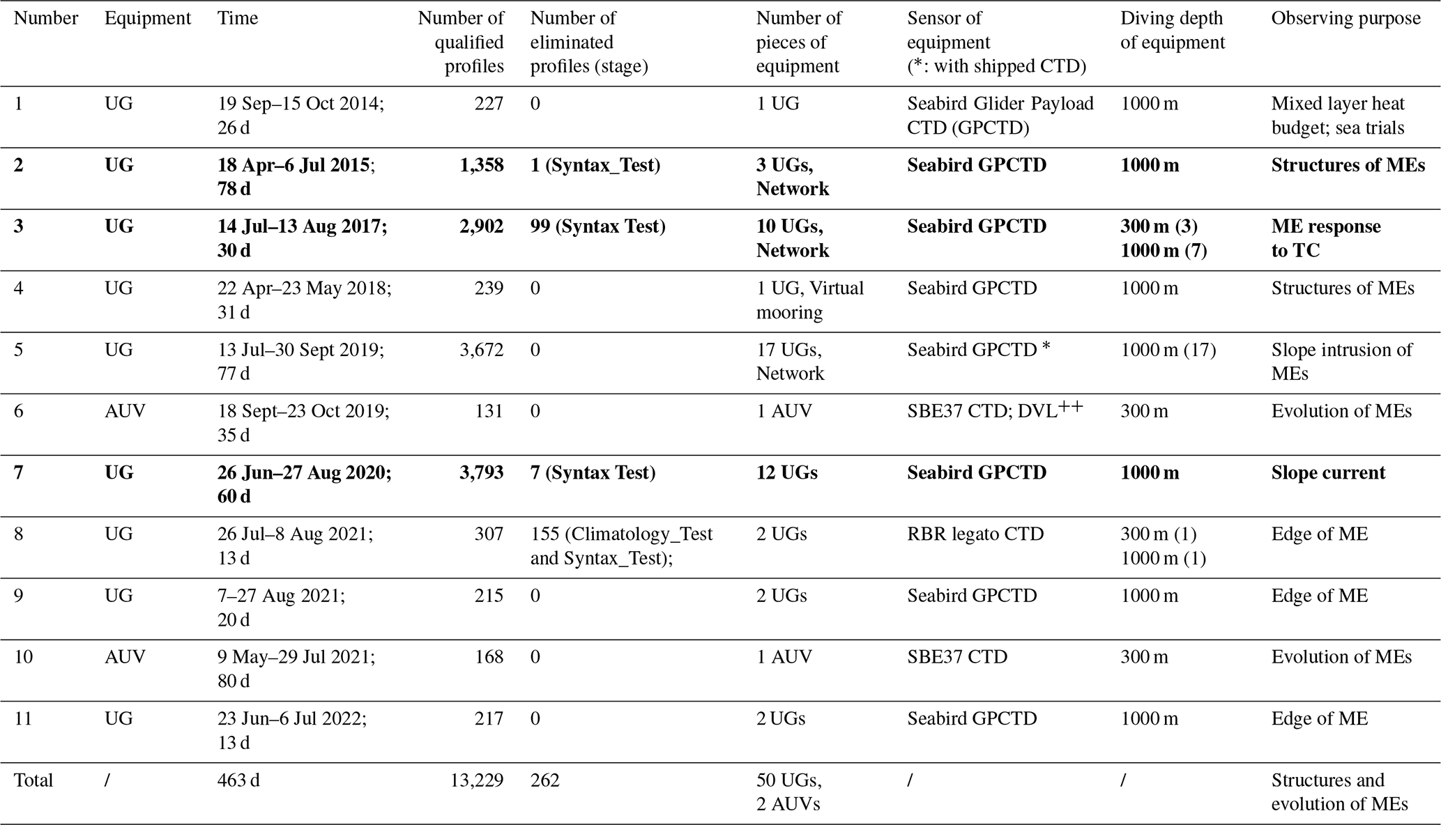
ME: mesoscale eddy; AUV: autonomous underwater vehicle; UG: underwater glider.

2 Datasets

2.1 UG and AUV experiment sites

Our experimental design specifically targeted ME evolution and submesoscale process characterization. This study employs two types of Chinese-developed UG platforms: “Sea-Wing” (Yu et al., 2011) and “Petrel” (Wu et al., 2011). Since 2014, we have conducted 11 field campaigns in the northern SCS, deploying 50 UGs and two AUVs to collect 13 491 temperature–salinity profiles. Platform deployment parameters, including the deploying time, installed sensors, and diving depths of UGs/AUVs for each experiment are shown in Table 2. Complete mission metadata (vehicle serial number, waypoints, matching time, latitude, and longitude) are archived in the data using the *.nc format. The bold terms in Table 2 highlight the UG arrays consisting of ≥ 3 units. Notably, in the experiments of 2017, 2019, and 2020, more than 10 UGs were deployed to resolve the three-dimensional structures of the MEs.

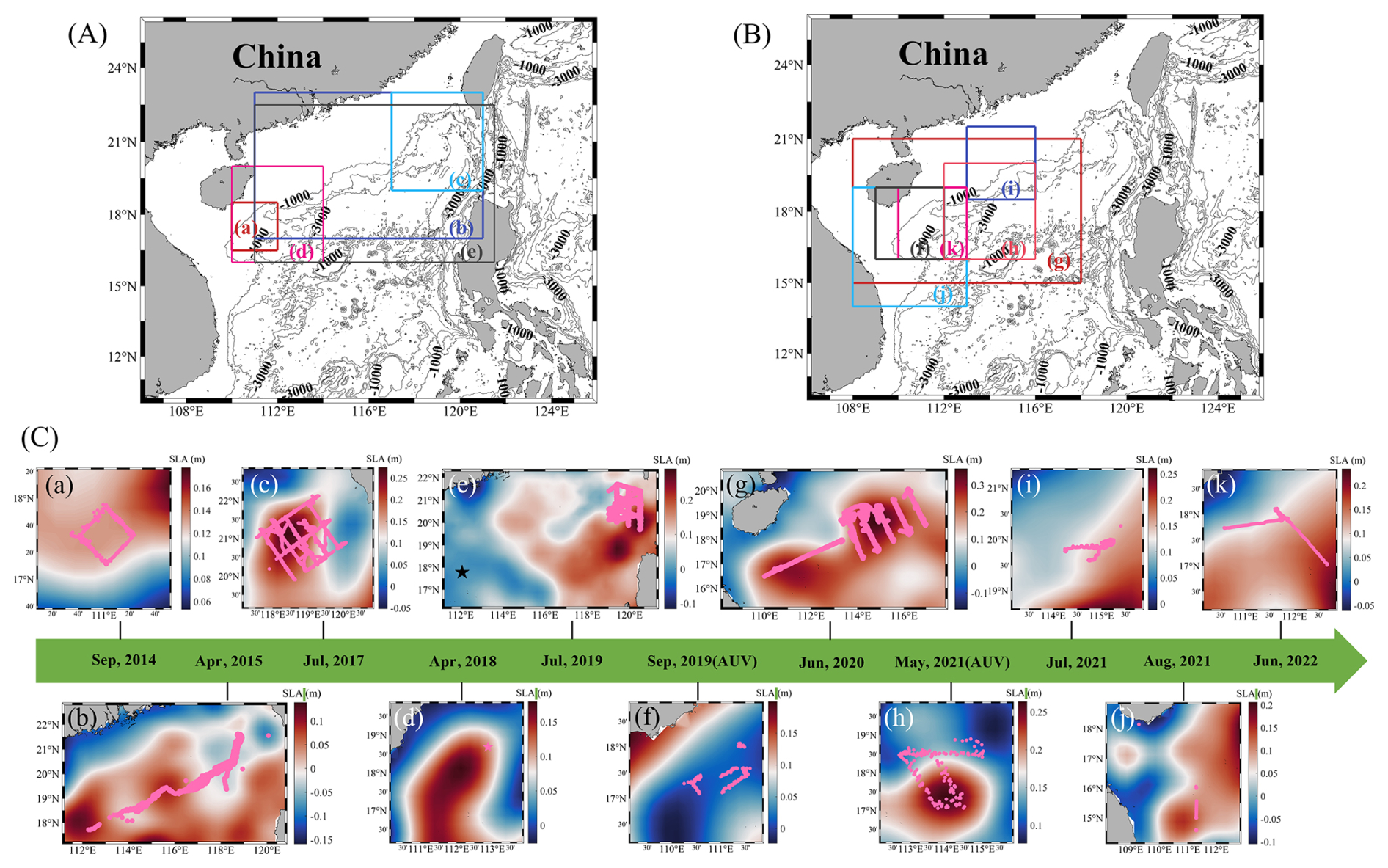
Figure 1 Underwater glider (UG) and autonomous underwater vehicle (AUV) observation sites. (a) Observation area for subplots (c.a)–(c.e); (b) area for subplots (c.f)–(c.j). The gray lines in (a) and (b) are the water depths. (c.a)–(c.k) Observation stations (pink dots) with mean sea level anomalies (shading colors). The observation times are (c.a) September 2014; (c.b) April 2015; (c.c) July 2017; (c.d) April 2018; (c.e) July 2019; (c.f) September 2019; (c.g) June 2020; (c.h) May 2021; (c.i) July 2021; (c.j) August 2021; and (c.k) June 2022.

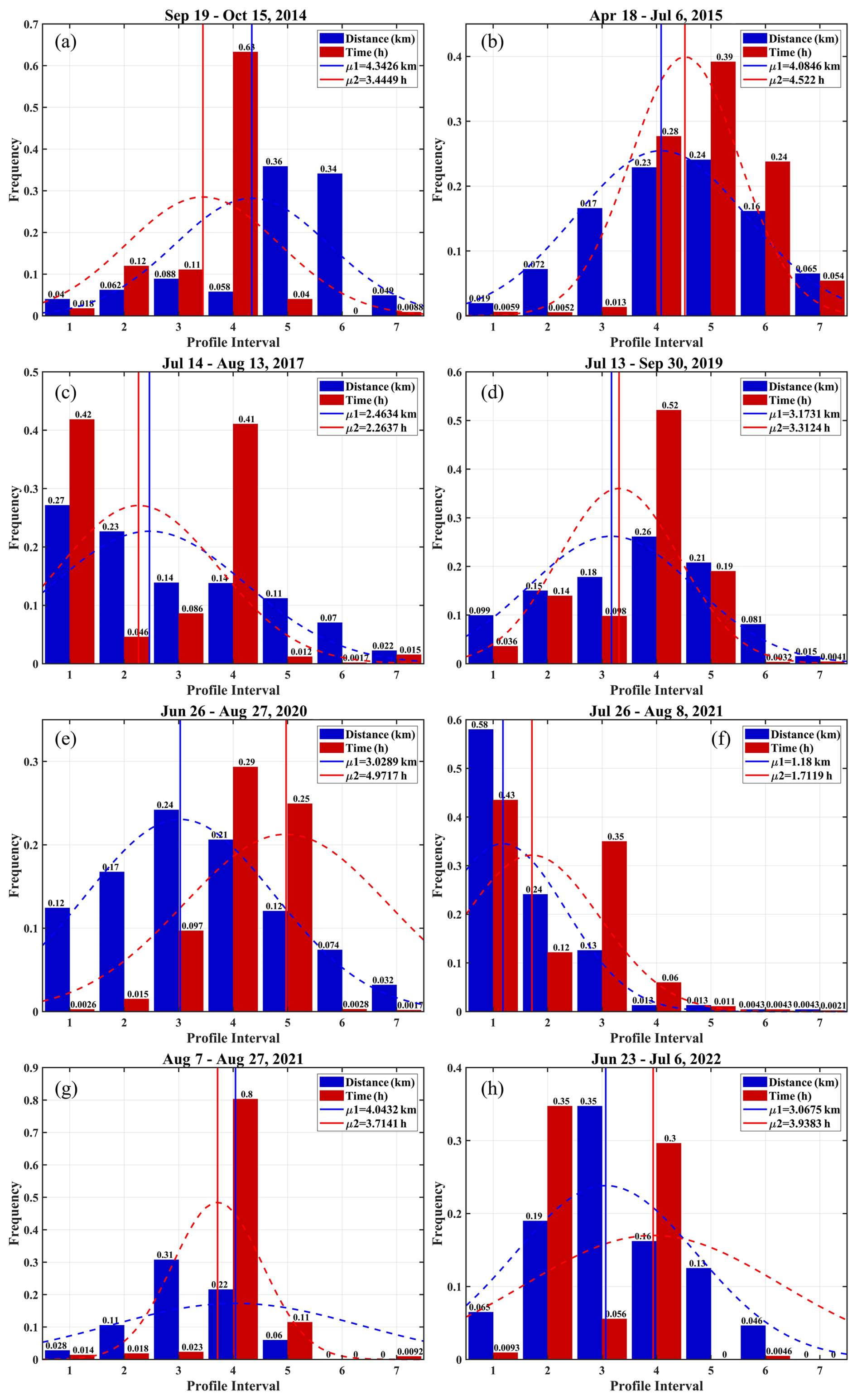
Figure 2 Frequency of spatial (blue bar) and temporal (red bar) sample intervals. “Profile interval” indicates the spatial interval (red) and temporal interval (blue). Bars are the probabilities. Dashed lines are normal distributions of the spatial (red) and temporal (blue) intervals. Mean values of the spatial and temporal intervals are depicted by the red and blue solid lines, respectively. The observation times are (a) September 2014; (b) April 2015; (c) July 2017; (d) July 2019; (e) June 2020; (f) July 2021; (g) August 2021; and (h) June 2022.

2.2 Intercomparison of UG and AUV resolutions

The trajectories of AUVs and UGs are depicted in Fig. 1. Each trajectory is superimposed on sea level anomaly (SLA) fields. The maximum absolute value of an SLA is the ME center. Note that all the UGs and AUVs crossed MEs. Spatio-temporal sampling characteristics are presented in Fig. 2. The horizontal resolution reveals two distinct regimes: 4–7 km resolution dominated the 2014, 2015, and 2019 campaigns (blue histograms), while sub-3 km sampling was achieved in the other years. The temporal sampling intervals exhibited similar bimodal distribution, reaching an optimal 1–2 h cadence during the 2017, July 2021, and 2022 deployments (Fig. 2c, f, and h), compared to the 4–7 h resolutions in the remaining experiments. This observational matrix demonstrates that 100 % of datasets resolve ME-scale dynamics (50–300 km spectral range), while 40 % of campaigns attained sufficient resolution to capture submesoscale features (< 3 km; < 4 h characteristic scale) through synergistic UG/AUV coordination.

3 Data quality control method

Prior to investigating the three-dimensional structures of MEs, we performed rigorous data quality control (QC) for the UG and AUV datasets.

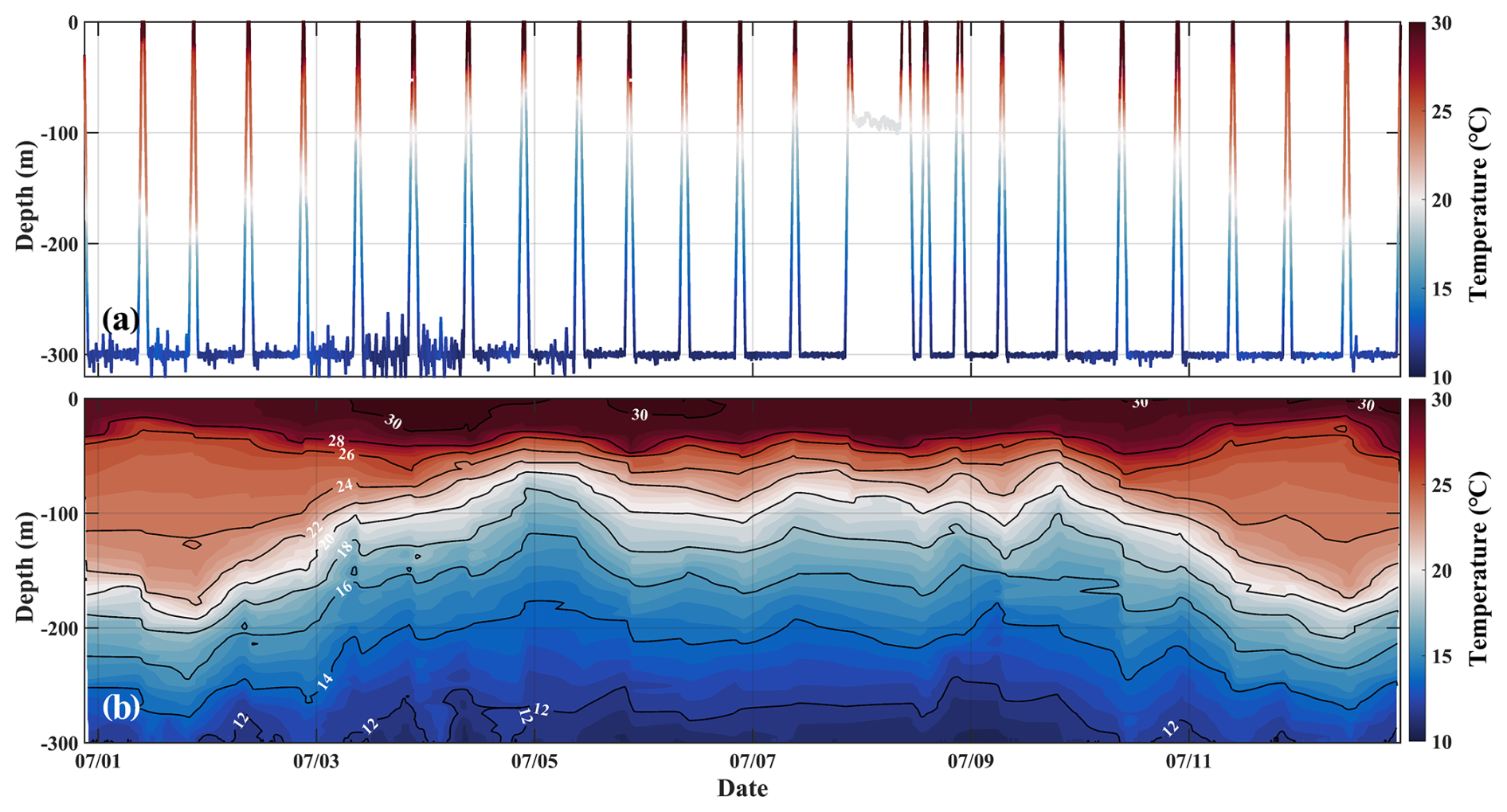
Figure 3 Illustration of (a) original and (b) interpolated temperature data after quality control. The AUV observation period is July 2021. AUV: autonomous underwater vehicle.

3.1 UG data quality control

Two Chinese UGs named “Sea-Wing” and “Petrel” were employed in this study. These platforms integrate communication and navigation subsystems comprising iridium satellite communication devices, wireless communication devices, a precision navigation attitude sensor, a Global Positioning System (GPS) device, a pressure sensor, an obstacle avoidance sonar, and a CTD sensor with a 6 s sampling interval.

Before investigating oceanic phenomena, we performed data quality control following the integrated ocean observing system (IOOS) standard. The QC procedure for UGs (https://repository.oceanbestpractices.org/handle/11329/289?show=full last access: 17 October 2024) includes nine steps: (1) Timing/gap test: this test determines that the profile has been received within the expected time window and has the correct time stamp. (2) Syntax test: this test ensures the structural integrity of data messages. (3) Location test: this tests if the reported physical location (latitude and longitude) is within the reasonable range determined by the operator. (4) Gross range test: this test ensures that the data points do not exceed the minimum/maximum output range of the sensor. (5) Pressure test: this tests if the pressure records increase monotonically with depth, sorts the vertical depth values, and removes any duplicate depth values. The data obtained after steps (1)–(5) are directly output by the UGs. (6) Climatology test: this tests if the data points are within the seasonal expectation range. (7) Spike test: this tests if the data points exceed the selected threshold compared to adjacent data points, excluding the data with temperature–salinity larger than 35°/35 psu. (8) Rate of change test: this tests if the rate of change in the time series exceeds the threshold determined by the operator. (9) Flat line test: this is a test for continuously repeated observations of the same value, which may be the result of sensor or data collection platform failure. Post-stage (6) and (7) data are designated as *_RO (remove outliers), while the outputs of stages (8) and (9) generate *_TSD (triple standard deviation) following 3σ outlier exclusion.

We performed cross-validation using the UG-observed temperature and salinity profiles and shipborne CTD cast data for July 2019 (Fig. 1e, black star, and Fig. 4). Quantitative analysis revealed that the mean bias of the temperature is 0.05 °C and that of the salinity is 0.01 psu. The vertical temperature–salinity profiles observed by the ship and UG are consistent, supporting the notion that the data are credible.

3.2 AUV data quality control

Both CTD and GPS instruments were installed on the “Sea-Whale 2000” AUV. The platform was designed by the Institute of Shenyang Automation, Chinese Academy of Sciences. It could operate in two modes: “sawtooth” mode and “cruise” mode at a specific depth of 300 m (Huang et al., 2019).

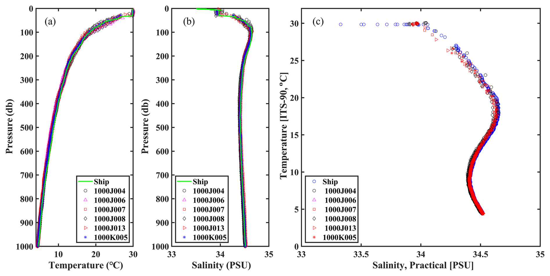
Figure 4 Comparison of (a) temperature, (b) salinity, and (c) temperature–salinity scatter plots between ship-installed CTD and AUV-installed CTD at station (17.7778° N, 112.0661° E). Green line in (a) and (b) is the ship-measured values. The dot, pink triangle, red square, diamond, red triangle, and blue star correspond to UGs named 1000J004, 1000J006, 1000J007, 1000J008, 1000J013, and 1000K005, respectively.

For the “sawtooth” mode data, we applied identical quality control protocols as described in Sect. 3.1 for UGs (Figs. 3 and 4). In “cruise” mode, the AUV navigates at a depth of around 300 m. Following Qiu et al. (2020), we first transformed the temperature and salinity at depth z to those at 300 m using a linear regression method ($T^{\prime }=\mathrm{0.008}{z}^{\prime }+\mathrm{0.017};S^{\prime }=-\mathrm{0.0002}{z}^{\prime }+\mathrm{0.0006}$):

$$\begin{array}{}\text{(1a)}& {\displaystyle }& {\displaystyle }{T}^{\prime }=T_z-T_{\text{mean}},\text{(1b)}& {\displaystyle }& {\displaystyle }{S}^{\prime }=S_z-S_{\text{mean}},\end{array}$$

where T_mean is averaged using a 10-point smoothed average, which could maintain the spatial variations from 20 to 30 km. The depth anomaly is defined as the measured depth minus 300 m, i.e., $z^{\prime }=z-\mathrm{300}$, and the temperature and salinity anomalies are defined as T^′ and S^′, respectively. Validation against the potential temperature algorithm demonstrated that the temperatures reconstructed at 300 m were highly consistent.

3.3 Density derived from temperature and salinity

Seawater density (ρ, in kg m⁻³) was computed based on temperature (T, in °C), salinity (S, in psu), and pressure (P, in dbar) using the UNESCO international equation of state (Fofonoff and Millard, 1983). The UNESCO formula provides a simplified approach to estimate seawater density as follows:

$$\begin{array}{}\text{(2a)}& {\displaystyle }\mathit{\rho }(S,T,P)={\displaystyle \frac{{\mathit{\rho }}_{\mathrm{0}}(S,T)}{\mathrm{1}-\frac{P}{K(S,T,P)}}},\text{(2b)}& {\displaystyle }\begin{array}{rl}{\mathit{\rho }}_{\mathrm{0}}(S,T)=& {\mathit{\rho }}_{\text{sw}}\left(T\right)+\left(b_{\mathrm{0}}+b_{\mathrm{1}}{T}_{\mathrm{68}}+b_{\mathrm{2}}{T}_{\mathrm{68}}^{\mathrm{2}}+b_{\mathrm{3}}{T}_{\mathrm{68}}^{\mathrm{3}}\right.\\ & \left.+b_{\mathrm{4}}{T}_{\mathrm{68}}^{\mathrm{4}}\right)S+\left(c_{\mathrm{0}}+c_{\mathrm{1}}{T}_{\mathrm{68}}+c_{\mathrm{2}}{T}_{\mathrm{68}}^{\mathrm{2}}\right)\\ & \times S\sqrt{S}+d_{\mathrm{0}}{S}^{\mathrm{2}},\end{array}\text{(2c)}& {\displaystyle }{\mathit{\rho }}_{\text{sw}}\left(T\right)=a_{\mathrm{0}}+a_{\mathrm{1}}{T}_{\mathrm{68}}+a_{\mathrm{2}}{T}_{\mathrm{68}}^{\mathrm{2}}+a_{\mathrm{3}}{T}_{\mathrm{68}}^{\mathrm{3}}+a_{\mathrm{4}}{T}_{\mathrm{68}}^{\mathrm{4}}+a_{\mathrm{5}}{T}_{\mathrm{68}}^{\mathrm{5}},\text{(2d)}& {\displaystyle }{T}_{\mathrm{68}}=T\times \mathrm{1.00024},\end{array}$$

where $K(S,T,P)$ is the secant bulk modulus and a₀ and others are coefficients. The coefficients follow the original formulation, accounting for nonlinear compressibility effects.

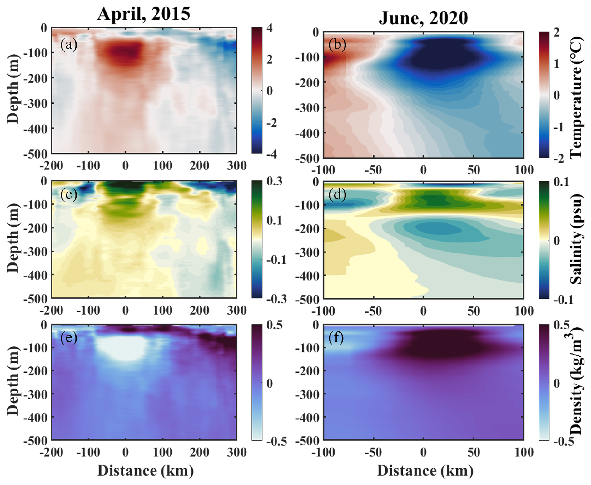
Figure 5 Contours of the (a) and (b) temperature anomaly, (c) and (d) salinity anomaly, and (e) and (f) density anomaly in April 2015 (a, c, and e) and June 2020 (b, d, and f). The contours were generated by interpolating the original data points.

4 Data application

4.1 Subsurface MEs observed by UGs and AUVs

Glider arrays successfully captured the full-depth thermohaline signatures of both warm and cold eddies through cross-eddy transects (Fig. 4). In April 2015, one UG deployment crossed a warm eddy and observed a subsurface warm core (Figs. 1b and 5a), corresponding to the subsurface eddy (50–500 m depth, 100 km radius) as described by Shu et al. (2016). Qiu et al. (2019b) utilized this dataset to investigate the asymmetry structures of this subsurface eddy, suggesting that the centrifugal force should be taken into account when revealing the velocity of MEs, i.e., gradient wind balance theory. June 2020 glider observations captured a subsurface cold eddy exhibiting pronounced thermohaline anomalies within the main pycnocline layer (Figs. 1g and 5d–f). This density-compensated structure, defined as local deviations from zonal mean conditions, manifested through compensating for temperature and salinity anomalies that generated a baroclinic density core penetrating the upper 500 m. The colocated thermohaline signatures demonstrate the UG's capability to resolve three-dimensional eddy characterization, including core localization, spatial footprint delineation, and dynamic intensity assessment.

Both UGs and AUVs demonstrate the ability to monitor the temporal evolutions of subsurface MEs. During their developmental stages, these vortices exhibit morphological instabilities that induce cross-slope transport along continental margins (Wang et al., 2018; Su et al., 2020; Qiu et al., 2022) while simultaneously generating submesoscale processes through frontal instability (Dong and Zhong, 2018; Yang et al., 2019). To capture the eddy evolution process, we executed five successive AUV transects along rectangular trajectories across an anticyclonic ME during May to July 2021 (Fig. 1h), supported by the National Key Research and Development Program.

Figure 6 illustrates a subsurface-intensified anticyclone occupying the 50–200 m depth stratum, exhibiting weakened stratification with a reduced Brunt–Väisälä frequency squared value ($N^{\mathrm{2}}=\frac{\mathrm{1}}{\mathit{\rho }}\frac{\mathrm{d}\mathit{\rho }}{\mathrm{d}z}<{\mathrm{10}}^{-\mathrm{4}}$). The AUV mission was divided into five discrete phases: T1 (8–11 June), T2 (19–23 June), T3 (29 June-4 July), T4 (10–15 July), and T5 (21–26 July). Delineating the eddy boundaries using isopycnals at 22.5 and 23.5 kg m⁻³, we quantified temporal variations in the eddy area and thermal properties. A progressive decline in both areal extent and mean temperature occurred between T1 and T3, followed by subsequent recovery from T4 to T5, indicating distinct weakening and reintensification phases. This life cycle aligns with Qiao et al.'s (2023) trajectory analysis documenting eastward propagation during T1–T3 and topographic trapping during T4 and T5.

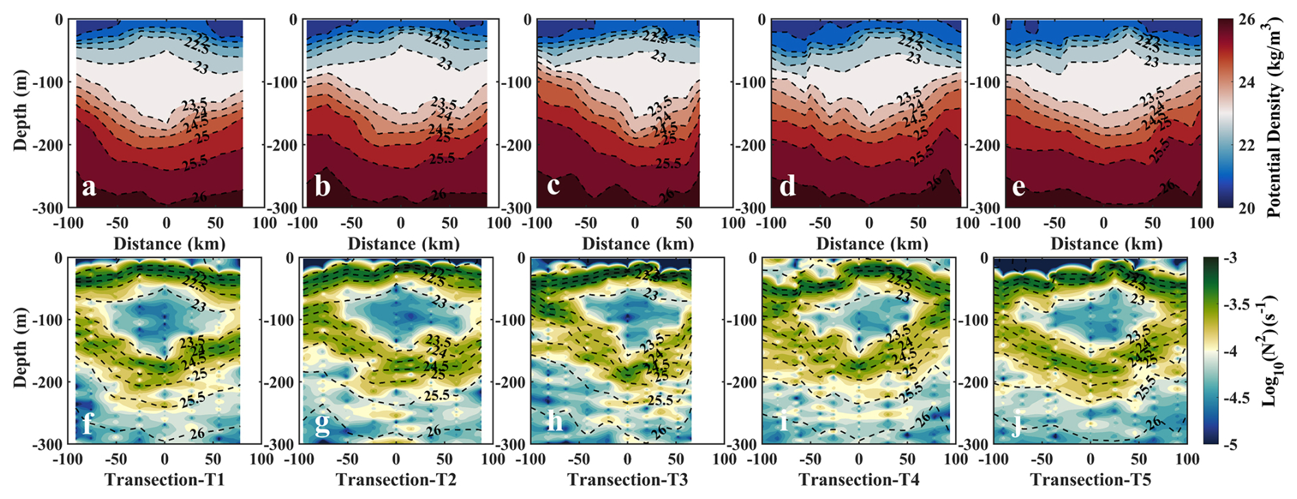
Figure 6 The profiles of density (a–e) and Brunt frequency (f–j) during (a, f) T1, (b, g) T2, (c, h) T3, (d, i) T4, and (e, j) T5 in 2021, which correspond to 06/08–06/11, 06/19–06/23, 06/29–07/04, 07/10–07/15, 07/21–07/26, respectively. The contours were generated by interpolating the original data points.

4.2 Vertical tilt of MEs at different life stages observed by UGs

Coordinated glider deployments were executed in 2015, 2017, 2019, and 2020 to resolve ME dynamics. The complete ME life cycle progresses through four distinct phases, i.e., birth, development, maturity, and dissipation stages (Zhang and Qiu, 2018; Yang et al., 2019), with each phase exhibiting different kinetic energy budgets. The Luzon Strait serves as an eddy birth zone, where the Kuroshio branch intrudes the SCS (Chen et al., 2011; Su et al., 2020). After birth, most of the eddies move westward to the continental shelf zone under the modulation of a Rossby wave before finally dissipating in the Dongsha Islands and Xisha Islands or merging with other eddies (Yang et al., 2019; Su et al., 2020; Qiu et al., 2022).

These deployments of AUVs and UGs enabled three-dimensional structural characterization across the ME life stages. Quality-controlled temperature–salinity profiles were interpolated into 1 km × 1 km × 1 m grids prior to density (ρ) computation. Assuming geostrophic balance, the geostrophic velocity, v_g, could be derived under the force balances between the pressure gradient and Coriolis forces:

$$\begin{array}{}\text{(3)}& v_{\mathrm{g}}\left(xyz\right)=v_{\mathrm{0}}-{\displaystyle \frac{g}{f{\mathit{\rho }}_{\mathrm{0}}}}\underset{z\mathrm{0}}{\overset{z}{\int }}\left({\displaystyle \frac{\partial \mathit{\rho }(x,y,z)}{\partial x}}+{\displaystyle \frac{\partial \mathit{\rho }(x,y,z)}{\partial y}}\right)\mathrm{d}z,\end{array}$$

where ρ₀ is the referenced water density, f is the Coriolis frequency, and v₀ (set to 0) represents the referenced geostrophic velocity at depth 1000 m.

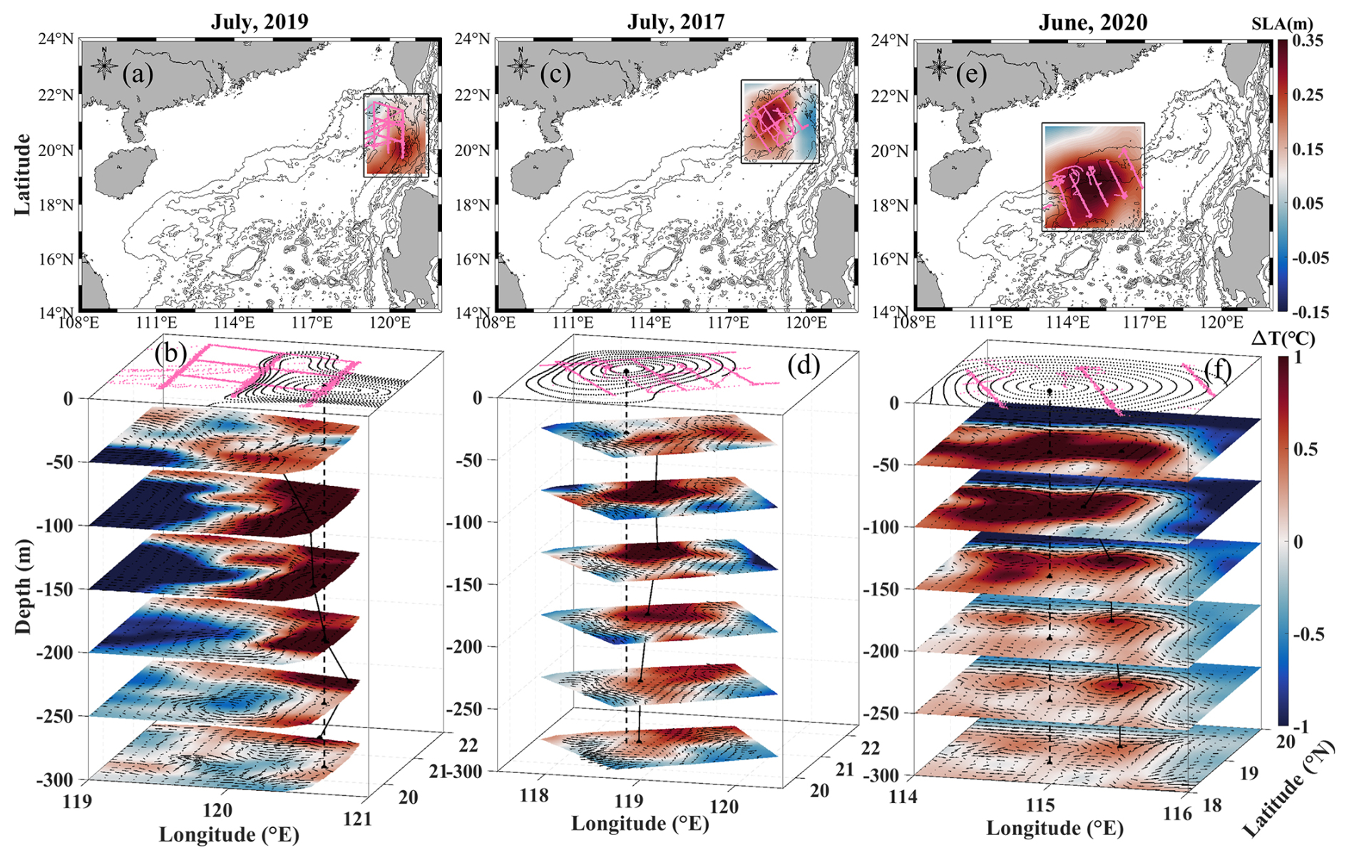
Figure 7 Eddy structures during periods of (a, b) eddy birth, (c, d) westward movement, and (e, f) dissipation along the slope. Sea level anomaly (SLA) and UG positions are superimposed in the upper panels (a, c, and e); isobaths are represented by solid lines. The UG-observed temperature and derived geostrophic velocities are shown in the 3D plots (b, d, and f). Pink lines are the tracks of UGs. Dashed lines denote the centers of mesoscale eddies from SLA fields, and solid lines show the centers of the warm cores at each depth. UG: underwater glider. The contours were generated by interpolating the original data points.

The July 2019 deployment (12 UGs, 120° E) observed the three-dimensional temperature and geostrophic velocity structures of an ME in the birth stage and captured the subsurface warm core exhibiting a northeastward vertical tilt (solid black line in Fig. 7). The July 2017 observations (10 UGs, 119° E) revealed a developing eddy that exhibited an eastward tilt through a 500 m water column, which may be attributed to combined forcing from westward-propagating Rossby waves and background current shear (e.g., Qiu et al., 2015; Zhang et al., 2016), as well as thermal front advection (e.g., Bonnici and Billant, 2020; Gaube et al., 2015). Throughout this experiment, the UGs encountered the tropical storm “Haitang”, resulting in the ME undergoing horizontal deformation and giving rise to submesoscale processes (Yi et al., 2022; Yi et al., 2024).

The June 2020 observations (12 gliders; Figs. 1g and 6e–h) documented a dissipating anticyclone with a southwestward tilt from 500 m to the surface (Fig. 7e and f). This kind of southwestward vertical tilt was revealed in a numerical model, which showed that the steep topography caused asymmetries of the velocities within the MEs (Qiu et al., 2022). The June 2021 AUV measurements (Qiao et al., 2023; Fig. 1h) further captured an eastward movement of the ME, which was dominated by wave-current interactions.

4.3 Submesoscale instabilities at the edge of MEs observed by UGs

Submesoscale processes usually occur within MEs, either at the eddy peripheries (front; filament) or entrained in the eddy center, in terms of spiral structures or “eye-cat” structures (Zhang and Qiu, 2018; Ni et al., 2021; Hu et al., 2023; Qiu et al., 2024a). These processes facilitate bidirectional energy transfers, driving forward cascades to dissipating scales through symmetric and centrifugal instabilities while simultaneously energizing inverse energy pathways to MEs via mixed-layer baroclinic instabilities (i.e., Fox-Kemper et al., 2008; McWilliams, 2016). Conventional Argo floats, constrained by 10 d sampling intervals, provide insufficient data to resolve rather short-duration features. Recent technological advancement reveals diverse observational capabilities. For example, Lagrangian platforms, like NAVIS floats, have identified frontal genesis dominated by mixed-layer baroclinic instability (Tang et al., 2022), while glider arrays employing virtual mooring configurations achieve Eulerian frontal characterization through programmable sampling strategies (Qiu et al., 2019a; Shang et al., 2023). This methodological contrast highlights glider advantages in enabling simultaneous cross-front and along-front measurements through active navigation, overcoming the spatial limitations inherent to passive Lagrangian drifters.

Our observational dataset reveals that 40 % of UG missions resolved submesoscale processes (< 3 km horizontal resolution, < 4 h temporal resolution; Fig. 2). To demonstrate this operational advantage, we analyzed two representative cases of submesoscale instabilities along ME peripheries.

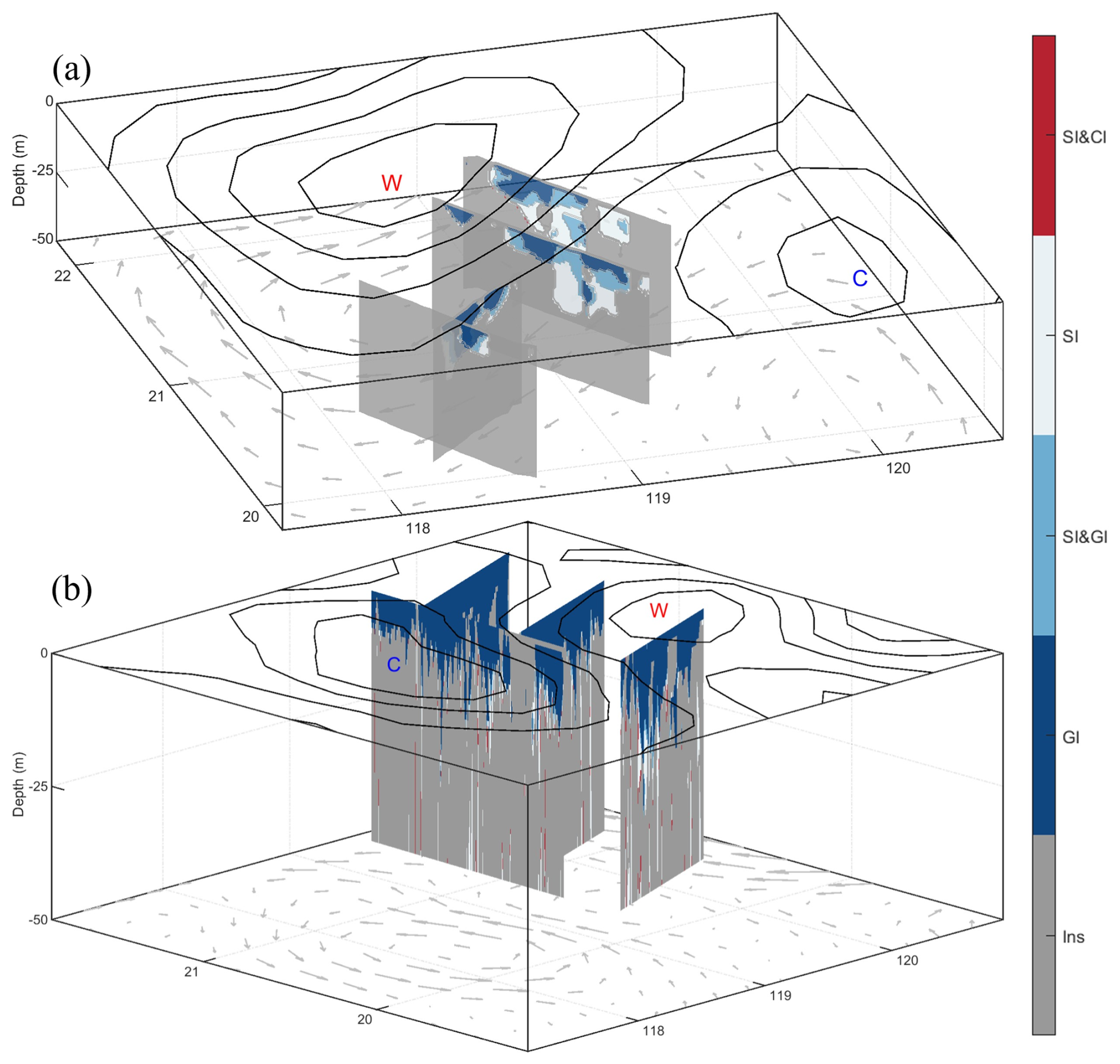
Figure 8 Analyzed submesoscale instabilities at the edge of mesoscale eddies in (a) 2017 and (b) 2019. SI: symmetric instability; CI: centrifugal instability; GI: gravity instability; W: anticyclonic eddy; C: cyclonic eddy. Isolines are the sea level anomalies, and vectors are the geostrophic velocities. The contours were generated by interpolating the original data points.

The 2017 deployment illustrates multi-platform sampling strategies, with four UGs strategically positioned at an anticyclonic ME boundary (Fig. 8a). Three UGs executed cross-front transects, while one maintained along-front tracking, enabling comprehensive instability characterization through the Richardson number phase angle, ϕ_Ri, defined as,

$$\begin{array}{}\text{(4a)}& {\displaystyle }& {\displaystyle }{\mathit{\varphi }}_{Ri}={\text{tan}}^{-\mathrm{1}}\left(-{\displaystyle \frac{\mathrm{1}}{Ri}}\right)={\text{tan}}^{-\mathrm{1}}\left({\displaystyle \frac{{\left|\mathrm{\nabla }\cdot b\right|}^{\mathrm{2}}}{N^{\mathrm{2}}\cdot f^{\mathrm{2}}}}\right),\text{(4b)}& {\displaystyle }& {\displaystyle }Ri\approx R{i}_{\mathrm{g}}={\displaystyle \frac{N^{\mathrm{2}}}{{\left(\frac{\partial {\mathit{v}}_{\mathrm{g}}}{\partial z}\right)}^{\mathrm{2}}}}={\displaystyle \frac{N^{\mathrm{2}}\cdot f^{\mathrm{2}}}{{\left|\mathrm{\nabla }\cdot b\right|}^{\mathrm{2}}}}<{\displaystyle \frac{f}{{\mathit{\zeta }}_{\mathrm{g}}}}\text{ and }f\cdot {\mathit{\zeta }}_{\mathrm{g}}>\mathrm{0},\end{array}$$

where $b=-g\mathit{\rho }/{\mathit{\rho }}_{\mathrm{0}}$ is the buoyancy flux and g is the gravitational acceleration. $N^{\mathrm{2}}=\partial b/\partial z$ is the vertical buoyancy frequency. ζ_g=curl(v_g) is the vertical relative vorticity (Thomas et al., 2013). For anticyclonic eddies, inertial instability or symmetric instability occurs when −45° < ϕ_Ri<ϕ_c. ${\mathit{\varphi }}_c={\tan }^{-\mathrm{1}}(-(f+{\mathit{\zeta }}_{\mathrm{g}})/f)$ is the critical angle. Only symmetric instability occurs when −90° < ${\mathit{\varphi }}_{Ri}<-\mathrm{45}\mathit{°}$; symmetric instability or gravitational instability occurs when −135° < ${\mathit{\varphi }}_{Ri}<-\mathrm{90}\mathit{°}$; and gravitational instability occurs when −180° < ${\mathit{\varphi }}_{Ri}<-\mathrm{135}\mathit{°}$.

The 2017 dataset revealed coexisting gravitational, symmetric, and centrifugal-symmetric instabilities along the ME periphery (Fig. 8a). Figure 8b shows submesoscale instabilities in 2019. In this case, gravity instability dominates the upper mixed layer, while symmetric and centrifugal instabilities are not significant. These two cases provide us enough information to detect frontal genesis processes in Eulerian view, while NAVIS or Argo devices provide frontal information in Lagrangian view.

5 Data availability

The dataset of temperature–salinity observed by AUVs and UGs in this paper was deposited in the Science Data Bank, whose DOI is https://doi.org/10.57760/sciencedb.11996 (Qiu et al., 2024b). The dataset includes two files: “Grid_data” and “Observation_data”.

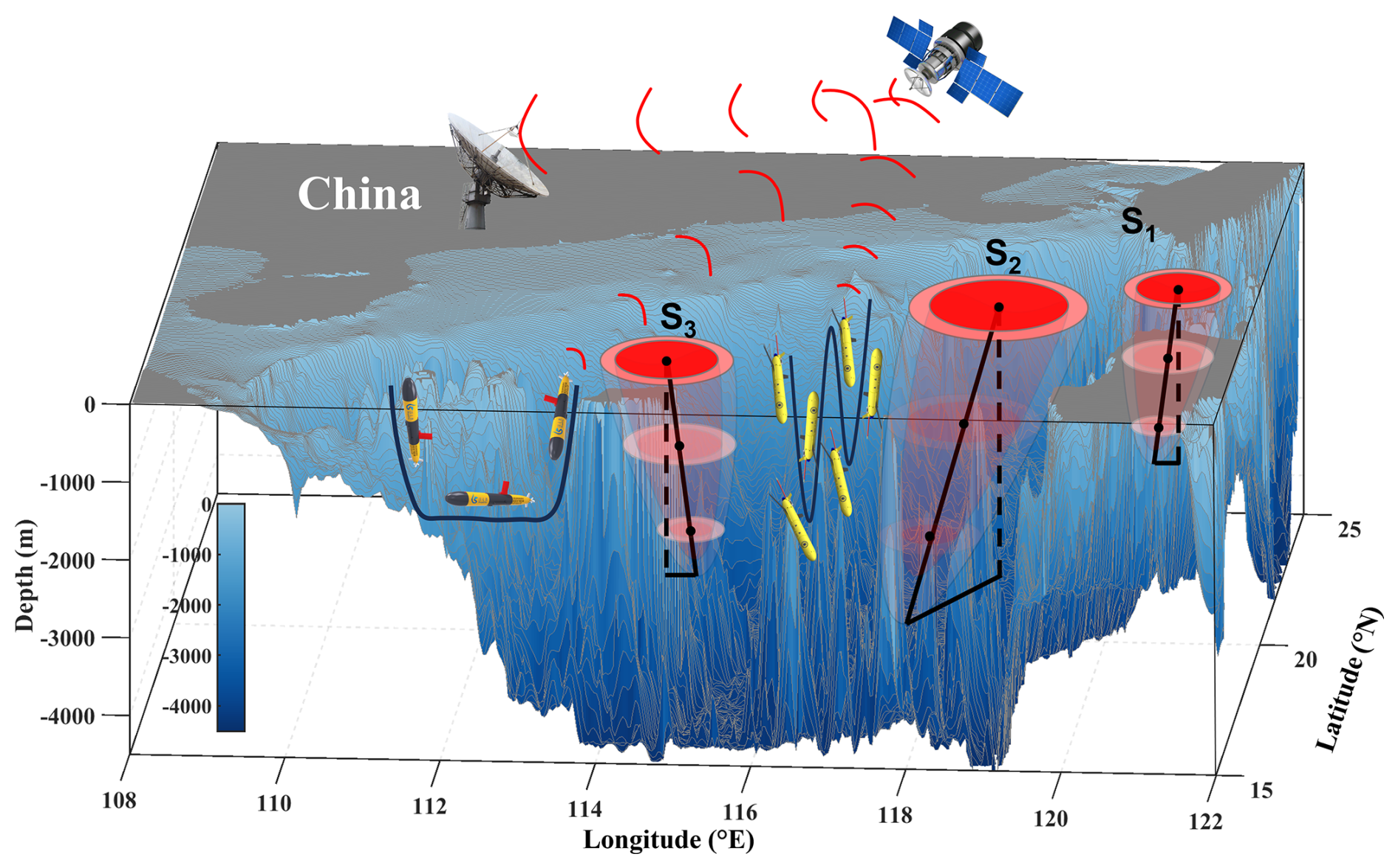
Figure 9 Schematic of UG operations conducted to observe mesoscale eddies at different life stages. S1: birth stage; S2: development/maturity stage; S3: dissipation stage.

6 Conclusions and potential future plan

Our 9-year AUV and UG observations yielded a dataset of high-resolution temperature and salinity profiles for the SCS. This comprehensive compilation comprises 13 491 profiles and covers 463 d' experiments, encompassing 11 experiments deploying 50 UGs and two AUVs. To our knowledge, this represents the first multi-platform dataset with sufficient spatio-temporal coverage in detecting the horizontal asymmetry, vertical tilt, temporal evolution, and life cycle of MEs (Fig. 9) while simultaneously capturing associated submesoscale processes. The dataset allows us to investigate the subsurface MEs, revealing eddy-current and eddy-topography interactions successfully. However, to quantify ME feedbacks based on the variability of larger-scale currents, i.e., western boundary current, long-term routine UG and AUV observations are needed in the future.

Beyond tracking MEs, UGs and AUVs have been proved to actively capture smaller-scale oceanic processes. Successful applications include internal tide (Gao et al., 2024) and turbulent dissipation rates by using turbulent parameterization schemes (Qi et al., 2020). Moreover, UGs/AUVs equipped with more sensors could provide us geochemical parameters (e.g., Yi et al., 2022), potentially enhancing coupled physical-biogeochemical model forecasting through data assimilation. More projects gathering an AUV network are ongoing and will be promoted in the future.

Operational challenges encountered during the program include the following: (1) under a strong background current, UGs and AUVs get disturbed and cannot follow the customized routes; (2) during extreme meteorological conditions, it is difficult for the piloting team to deploy and recover UGs and AUVs; and (3) data-receiving capacity depends on the satellite transmission capacity. If both the bio-chemistry and CTD data are included, the data resolution has to be lowered. Addressing these challenges requires synergistic collaboration between field operations teams, platform engineers, and dynamical oceanographers to optimize autonomous sampling systems.