LakeBeD-US: a benchmark dataset for lake water quality time series and vertical profiles

Water quality in lakes is an emergent property of complex biotic and abiotic processes that differ across spatial and temporal scales. Water quality is also a determinant of ecosystem services that lakes provide and is thus of great interest to ecologists. Machine learning and other computer science techniques are increasingly being used to predict water quality dynamics as well as to gain a greater understanding of water quality patterns and controls. To benefit the sciences of both ecology and computer science, we have created a benchmark dataset of lake water quality time series and vertical profiles. LakeBeD-US contains over 500 million unique observations of lake water quality collected by multiple long-term monitoring programs across 17 water quality variables from 21 lakes in the United States. There are two published versions of LakeBeD-US: the “Ecology Edition” published in the Environmental Data Initiative repository (https://doi.org/10.6073/pasta/c56a204a65483790f6277de4896d7140, McAfee et al., 2024) and the “Computer Science Edition” published in the Hugging Face repository (https://doi.org/10.57967/hf/3771, Pradhan et al., 2024). Each edition is formatted in a manner conducive to inquiries and analyses specific to each domain. For ecologists, LakeBeD-US: Ecology Edition provides an opportunity to study the spatial and temporal dynamics of several lakes with varying water quality, ecosystem, and landscape characteristics. For computer scientists, LakeBeD-US: Computer Science Edition acts as a benchmark dataset that enables the advancement of machine learning for water quality prediction.

1 Introduction

Water quality is a critical determinant of the ecosystem services provided by lakes (Keeler et al., 2012; Angradi et al., 2018). Water quality varies across spatial and temporal scales (Hanson et al., 2006; Langman et al., 2010; Soranno et al., 2017) as a result of a variety of interacting physical and biological processes. For example, hypolimnetic anoxia (low oxygen) in lakes reduces the available habitat for cold-water fish species (Arend et al., 2011; Jane et al., 2024). Anoxia can be fueled by the product of another water quality problem, the formation of toxic phytoplankton blooms (Jane et al., 2021). Both of these water quality phenomena emerge at the ecosystem scale as a consequence of multiple physical–biological interactions, driven by external nutrient loads and weather conditions (Paerl and Huisman, 2009; Snortheim et al., 2017; Ladwig et al., 2021; Jane et al., 2021). While there is mechanistic understanding of how these water quality phenomena evolve for well-studied lake systems, predicting their occurrence under scenarios of change or in large numbers of systems with sparse data remains challenging (Guo et al., 2021; Miller et al., 2023). To meet this challenge, we need scalable water quality models that are supported by observational data of sufficient spatiotemporal resolution to reproduce key water quality dynamics (Ejigu, 2024; Varadharajan et al., 2022).

Knowledge-guided machine learning (KGML) has emerged as a powerful technique for incorporating both ecological knowledge and observational data within a model (Karpatne et al., 2017, 2024). By fusing machine learning with physical and ecological principles, KGML has proven effective for assessing lake surface area change (Wander et al., 2024), modeling lake temperature (Read et al., 2019; Daw et al., 2014; Ladwig et al., 2024; Chen et al., 2024b), phytoplankton (chlorophyll) forecasting (Lin et al., 2023; Chen et al., 2024a), and predicting lake phosphorus concentrations (Hanson et al., 2020). Thus, a variety of modeling techniques within and beyond KGML are required to advance water quality understanding and prediction (Wai et al., 2022; Lofton et al., 2023). Creative approaches will likely spring from interdisciplinary collaborations of both lake ecologists and computer scientists (Carey et al., 2019) and will need diverse, high-volume, high-quality observational data that are easily accessible to researchers from multiple disciplines.

Predicting the evolution of water quality through time and space requires treating lakes as dynamical systems that operate across many scales. The nature of research project design lends itself to focusing on either the temporal scale or the spatial scale, making studies that address both scales extensively somewhat rare (but see Wilkinson et al., 2022; Zhao et al., 2023; Meyer et al., 2024). Datasets that capture spatial gradients (Soranno et al., 2017; Pollard et al., 2018), temporal gradients (Magnuson et al., 2006; Goodman et al., 2015), or both have been curated manually to produce harmonized derived products (Read et al., 2017). Few examples of lake water quality data exist that harmonize both manually sampled and autonomously sampled high-frequency data across key gradients in space and across decadal timescales.

A benchmark dataset for lake water quality that has well-resolved temporal data spanning multiple variables would be invaluable to both limnologists and computer scientists for simultaneously advancing both water quality modeling and KGML. Benchmark datasets are curated and cleaned datasets used in computation-heavy fields to test new operational methods and compare their performances (Peters et al., 2018). High-quality benchmark datasets require significant effort to create (Sarkar et al., 2020) but are of fundamental importance to the field of computer science (Li et al., 2024). Sarkar et al. (2020) and Weinstein et al. (2021) lay out many criteria for a quality benchmark dataset, which include the following.

• Relevance. Data must be well curated so as to be relevant for a specific phenomena. In this case, the dataset must contain lake water quality data.

• Representativeness. Data should contain examples from many relevant areas so as to be representative of a global distribution. In the case of water quality, this means data from lakes across geographic, trophic, and morphological gradients.

• Non-redundancy. The dataset should exclude duplicate data (i.e., every observation is unique).

• Experimentally verified. Data should be real observations, rather than generated from simulations. In the case of lake water quality, this means that all data are collected in situ.

• Scalability. The design of the dataset should allow the methods tested to vary in complexity. This requires a set of reasonable evaluation criteria and transparent scoring.

• Reusability. Data should be open-source, freely available, and shared in a manner such that the dataset can be used for other applications.

Benchmark datasets are becoming more prevalent in the field of ecology (e.g., Weinstein et al., 2021; Schür et al., 2023). Ecological benchmark datasets are vital as environmental data, including water quality data, exhibit properties such as prevalent missing values and non-normal distributions (Helsel, 1987; Lim and Surbeck, 2011) that are not typically represented in machine learning benchmark datasets. Benchmark datasets exist within the field of hydrology (e.g., Addor et al., 2017; Demir et al., 2022) and some recent limnology datasets advertise machine learning as a potential application (e.g., Spaulding et al., 2024), but benchmark datasets are rare in the field of limnology. This scarcity has caused some limnological studies to use non-limnological benchmark datasets to test their machine learning methods (e.g., Kadkhodazadeh and Farzin, 2021).

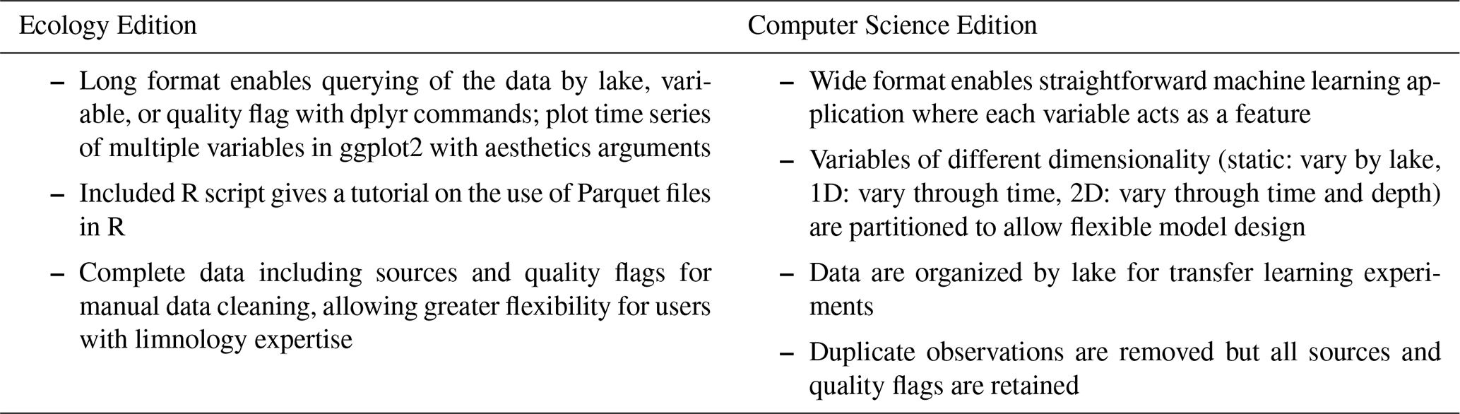
Table 1 Characteristics of the different formats of LakeBeD-US.

This paper introduces LakeBeD-US, a dataset of lake water quality time series and vertical profiles intended as a benchmark for comparative methodological analysis for water quality modeling. LakeBeD-US harmonizes water quality data from long-term water quality monitoring programs, including the North Temperate Lakes Long-Term Ecological Research program (NTL-LTER), the National Ecological Observatory Network (NEON), the Niwot Ridge Long-Term Ecological Research program (NWT-LTER), and the Carey Lab at Virginia Tech as part of the Virginia Reservoirs Long-Term Research in Environmental Biology (LTREB) site in collaboration with the Western Virginia Water Authority. To conform with the principles of FAIR (findable, accessible, interoperable, and reusable) data (Wilkinson et al., 2016), the data are accessible via digital object identifiers (DOIs), the contents are richly described in the metadata, and all provenance is documented for each data point. Data from 21 lakes are included. The lakes vary in size, geographic region, trophic status, and temporal coverage. LakeBeD-US is published in two forms, each with a unique DOI: LakeBeD-US: Ecology Edition (LakeBeD-US-EE; McAfee et al., 2024) is published in the Environmental Data Initiative repository, which is a repository of primarily ecological data (Gries et al., 2023). LakeBeD-US: Computer Science Edition (LakeBeD-US-CSE; Pradhan et al., 2024) is published in the Hugging Face repository, which is used heavily by scientists developing and testing machine learning algorithms (Jain, 2022; Yang et al., 2024). Both versions are published as Apache Parquet files, a space-efficient and programming-language-independent file type effective for storing time series data (Rangaraj et al., 2022). LakeBeD-US-CSE is derived from LakeBeD-US-EE with additional cleaning and reformatting as described in Sect. 2 of this paper.

2 Dataset components and assembly

The goal of LakeBeD-US is to feature data from a collection of well-observed lakes that showcase the varied morphological, geographical, anthropological, and biological characteristics of environments across the United States. To do this, we leveraged data collected by prominent long-term monitoring programs. The NTL-LTER sampling strategy focuses on heterogeneous lakes within the state of Wisconsin (Magnuson et al., 2006). NEON samples lakes across the continent, capturing additional climactic and land use gradients (Goodman et al., 2015). Green Lake 4 from the NWT-LTER was chosen as a representative of alpine lakes in the dataset, as it has been monitored for many years (Bjarke et al., 2021). Falling Creek Reservoir and Beaverdam Reservoir represent managed drinking water supply reservoirs (Carey et al., 2024) which may exhibit unique characteristics as a result of their human influence. The degree to which the lakes in LakeBeD-US vary is discussed further in Sect. 3.

The LakeBeD-US dataset is presented in two formats: the Ecology Edition (LakeBeD-US-EE; McAfee et al., 2024) and the Computer Science Edition (LakeBeD-US-CSE; Pradhan et al., 2024). LakeBeD-US-EE is formatted to support analyses of lake water quality by the limnology community, while LakeBeD-US-CSE is formatted for use with machine learning and KGML methods. The Ecology Edition is presented in a long format, with each water quality variable sharing columns such that variables of interest can be queried from the dataset using dplyr (Wickham et al., 2023) commands in R (R Core Team, 2023), and visualizing time series with common plotting tools like ggplot2 (Wickham, 2016) can be done efficiently. The Computer Science Edition is presented in a wide format where each water quality variable is presented in its own column, enabling their use as separate features in a machine learning model. More information about the two versions is presented in Table 1 and discussed further in Sect. 2.2.2.

2.1 LakeBeD-US: Ecology Edition

2.1.1 Source data harmonization

LakeBeD-US-EE was assembled by downloading the source data to R (version 4.3.3, R Core Team, 2023) using the “EDIutils” (version 1.0.3, Smith, 2023) and “neonUtilities” (version 2.4.2, Lunch et al., 2024) packages. The data were harmonized using the Tidyverse suite of packages (version 2.0.0, Wickham et al., 2019) before being exported to Parquet files with the “arrow” package (version 15.0.1, Richardson et al., 2024). The code to download and harmonize the data was written to search the source repository for the most updated version of the source data prior to harmonization. The specific version of the source data used is tracked in a separate table, listed in the code as the provenance object, which is manually checked for changes before further use of LakeBeD-US-EE.

During harmonization into the LakeBeD-US-EE format, all measurements of the same variable were converted into common units. The only exception to this is chlorophyll a, which comes in two types of units that are not directly comparable without additional analysis: relative fluorescence units (RFU) and micrograms per liter (µg L⁻¹). Most of the source data related to nutrients or chemistry were already reported in either µg L⁻¹ or milligrams per liter (mg L⁻¹), which were straightforward to convert from one to the other. Data reported in molar units or microequivalents were converted to mass concentration units. Photosynthetically active radiation (PAR) data reported in lux units were converted to micromoles per square meter per second ($\mathrm{\mu }\mathrm{mol}{\mathrm{m}}^{-\mathrm{2}}{\mathrm{s}}^{-\mathrm{1}}$) using the full sunlight conversion factor of 0.0185 (Thimijan and Heins, 1983).

2.1.2 Lake information table

The lake information table contains static attributes of the 21 lakes included in LakeBeD-US. These attributes include the monitoring program, latitude, longitude, elevation above sea level, lake surface area, mean and maximum depth, estimated hydrologic residence time, and any known manipulations of the lake performed by humans. These values were derived from published literature listing the attributes of each lake (listed in Sect. S2 in the Supplement). Mean depth values were calculated based on available bathymetry information (Carey et al., 2022) when no values were reported in the literature. The hydrologic residence times listed are estimates based on the range of times the lake exhibits (Flanagan et al., 2009; Gerling et al., 2014). An estimated hydrologic residence time was available for all lakes except for Fish Lake (Dane County, WI), a closed-basin lake with no surface water inflows or outflows. Elevations for each lake were obtained using the United States Geological Survey's (USGS) National Map Bulk Point Query Service (United States Geological Survey, 2024). While there is uncertainty associated with the USGS 3D Elevation Program (Stoker and Miller, 2022), we found that elevation values captured the ecologically relevant variation and closely matched many published values for the 21 lakes in LakeBeD-US. Sources for each specific attribute of a lake are listed as comments in the source code compiling the attributes and listed collectively in the provenance metadata of LakeBeD-US-EE.

2.1.3 High- and low-frequency observations tables

Observational data are compiled into two Parquet datasets: one representing data collected from a buoy-mounted sensor at a relatively high temporal frequency and the other collected by hand at a relatively low temporal frequency. The high- and low-frequency datasets use an identical format and can be easily merged if needed. However, there are many analytical considerations that differ between these temporal frequencies, so they are provided separately for LakeBeD-US-EE. The low-frequency observation table includes a larger suite of variables at a greater number of discrete depths along the water column.

Both the high- and low-frequency datasets are comprised of columns listing the source of a data point, date and time, the lake, depth, water quality variable, unit, observed value, and data flag. The data are provided in a long format for ease of querying the data by filtering with dplyr (Wickham et al., 2023) commands in R. All unit names were sourced from the QUDT (Quantities, Units, Dimensions and Types) ontology (FAIRsharing.org, 2022), with the exception of RFU which is not included in the ontology. Water quality variable names are defined in the metadata of both the LakeBeD-US-EE and LakeBeD-US-CSE datasets.

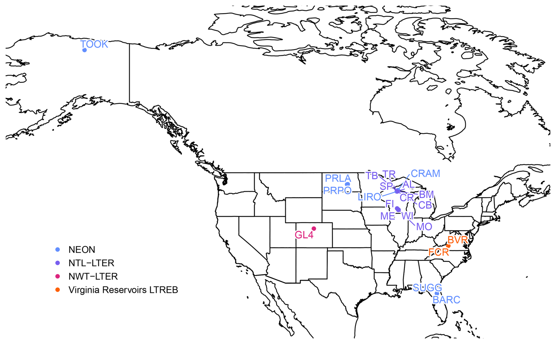
Figure 1 Locations and names of the 21 lakes included in LakeBeD-US. Lakes are monitored by the National Ecological Observatory Network (NEON, blue), the North Temperate Lakes Long-Term Ecological Research program (NTL-LTER, purple), the Niwot Ridge Long-Term Ecological Research program (NWT-LTER, pink), and the Carey Lab at Virginia Tech as part of the Virginia Reservoirs Long-Term Research in Environmental Biology (LTREB) site in collaboration with the Western Virginia Water Authority (orange). More information about each lake is included in Table 3.

2.1.4 Data flagging

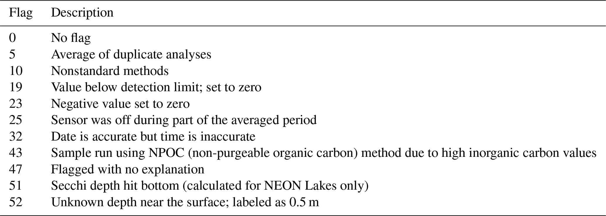
Each of the original data sources (listed in Sect. S1 in the Supplement) has data quality flagging systems that have been maintained for LakeBeD-US-EE (Table A3). We documented all of the data quality flags in the original data sources and assigned each unique type of quality flag a number, aligning common types between each source. These numeric flags for LakeBeD-US are documented in the included flag guide table (Fig. 3; Table A3). As data go through the harmonization workflow to be included in LakeBeD-US-EE, the original flag values are reassigned to align with the LakeBeD-US flag. There are 51 total unique flags among all of the data sources that were included in LakeBeD-US. Some of the data sources contain flags that are not defined in the metadata for those sources, in which case the data author was contacted and asked for a definition. Typically, these flags were errors in data entry and filtered out of LakeBeD-US. The exact depths at which some of the early buoy-mounted sensors were positioned were not documented and this institutional knowledge has been lost to time. Fortunately, documented protocols state that the sensors were mounted in the mixed surface layer of the lake. Thus, we have applied a depth value of 0.5 m to those observations with the flag 52 attached. The design of the flagging system in LakeBeD-US allows users to apply their own preferred level of uncertainty to their analysis. However, we suggest using the flags listed in Table 2 as guidance.

Table 2 Acceptable flag codes for selected data used in the LakeBeD-US-CSE benchmark. Not all the flag codes listed are relevant to the variables used in the benchmark task, but all are flags we would consider acceptable within quality control steps for most tasks using LakeBeD-US.

2.2 LakeBeD-US: Computer Science Edition

2.2.1 Transformation from LakeBeD-US-EE

LakeBeD-US-CSE was transformed from the observational data and lake attribute information of LakeBeD-US-EE. The original data were loaded with Python (version 3.12.4, Van Rossum and Drake, 2009) and transformed using pandas (version 2.2.2, The pandas development team, 2024; McKinney, 2010) and NumPy (version 2.1.1, Harris et al., 2020). Since the original data files were stored as Parquet files, additional dependencies such as fastparquet (version 2024.5.0, Durant and Augsperger, 2024) and PyArrow (version 17.0.0, Apache Arrow Developers, 2024) were required for pandas. The transformation process consisted of five major components: flag imputation, data cleaning, variable renaming, deduplication, and pivoting. The harmonization workflow is visualized in Fig. 2 and the steps taken in each component are outlined below.

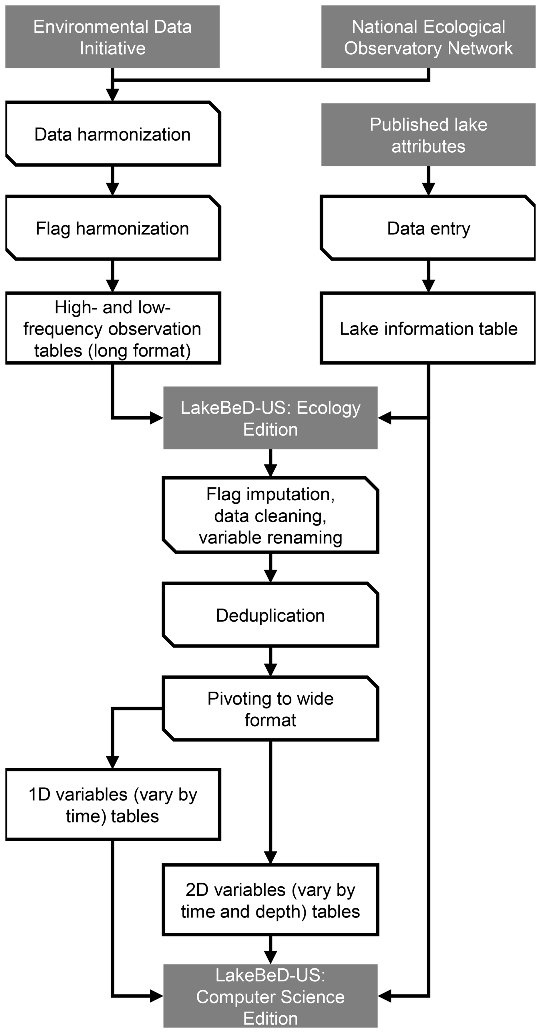
Figure 2 Harmonization workflow for LakeBeD-US. Boxes represent states of data and corner-snipped parallelograms represent processes. Gray boxes represent published products and sources of published products.

1. Flag imputation.. Observations with missing values for flag were assumed to be accurate observations and imputed with a flag value of 0.

2. Data cleaning. Some observations of 2D variables were assigned depth values of −99 to indicate an integrated (i.e., taken from multiple depths simultaneously) observation. We omit those observations as they are not directly comparable to discrete depth observations. It should be noted that several observations contain negative values for depth close to zero (on the order of $-{\mathrm{10}}^{-\mathrm{3}}$ to $-{\mathrm{10}}^{-\mathrm{7}}$ m) but are correct observations. Such observations come from artificial reservoirs where the water level fluctuates greatly. As such, the depths for those observations need to be calculated from the reference surface level, leading to some error in the depth measurement. It is permissible to round these values to zero if needed for simplification.

3. Variable renaming. The units column of the observational data in LakeBeD-US-EE was omitted in favor of listing the units in the metadata. However, chlorophyll a (chla) is reported in both RFU and µg L⁻¹ in the Ecology Edition. We separate this single variable with two units into chla_rfu and chla_ugl to distinguish between the two possible units of measurement for chlorophyll a.

4. Deduplication. The spatiotemporal nature of the data combined with flag values creates a bifurcation structure in the one-dimensional (1D, i.e., varying over time) variables and a trifurcation structure in the two-dimensional (2D, i.e., varying over time and depth) variables (see Sect. 2.2.2 for more information on variable types). A 1D observation can be indexed by datetime and flag, and a 2D observation can be indexed by datetime, depth, and flag. Multiple observations could be present at a given index. We combine multiple observations at an index into a single observation by calculating the median.

5. Pivoting. LakeBeD-US-EE is distributed in a “long” format where different variables are stored as a single column. This format was converted into a wide format with tabular data where each variable has its own column. For 1D variables, datetime and flag were used as pivot indices, variable was used to denote the different resulting columns for the variables, and observation was used to populate the columns with values. Pivoting of the 2D data was performed identically except for the pivot indices where datetime, depth, and flag were used.

2.2.2 File structure and components

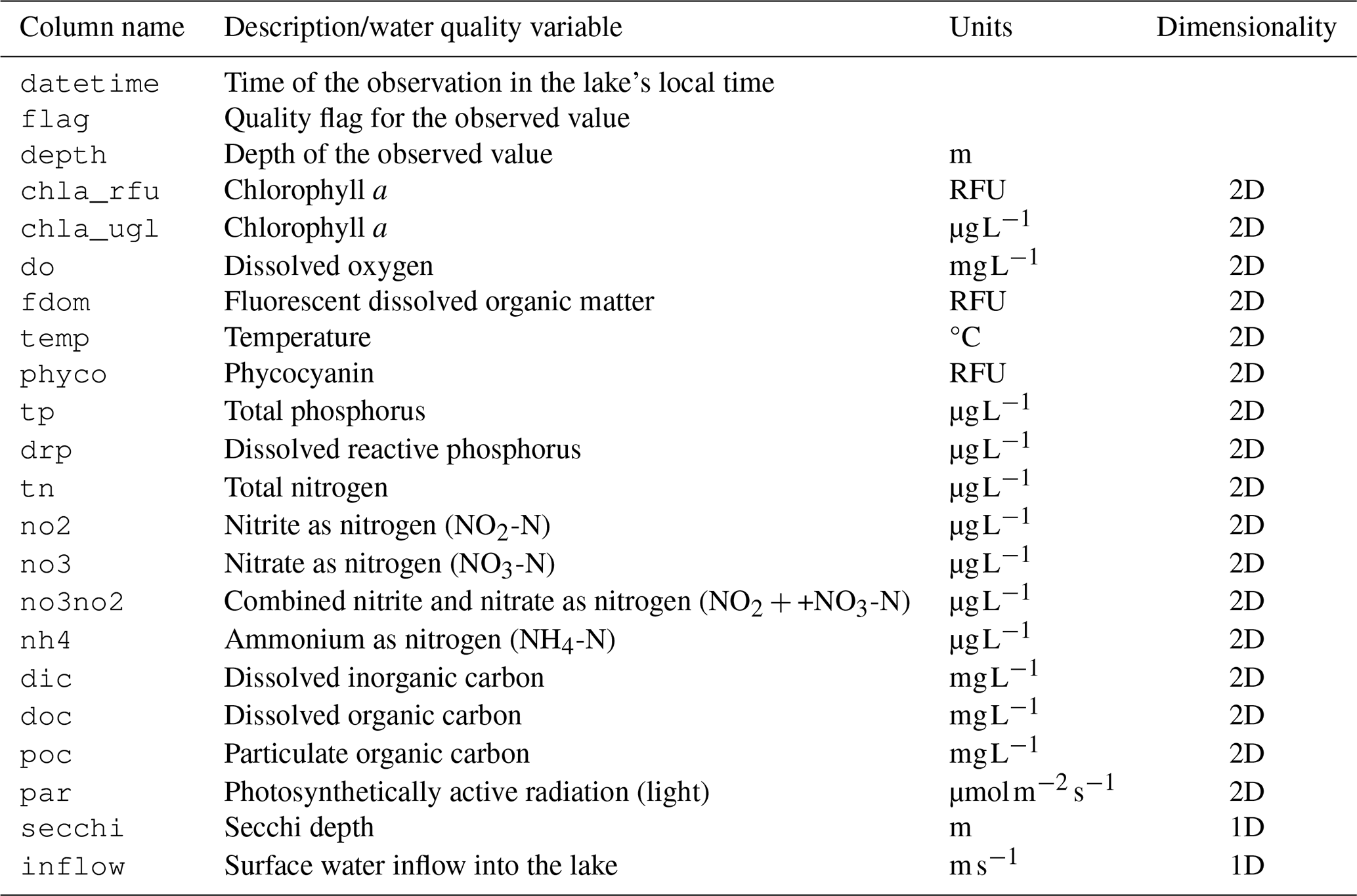
LakeBeD-US-CSE has a nested file structure as shown in Fig. 3. High- and low-frequency observational data are divided into two folders, each containing sub-folders for different lakes. Each lake's folder contains two tables: 1D variables and 2D variables. The lake information table from LakeBeD-US-EE is carried over to LakeBeD-US-CSE as a CSV (comma-separated value) file, while the 1D and 2D variable data are stored as Parquet files within the nested file structure. Static covariates are the lake attributes that generally remain constant over time, derived from the lake information table in LakeBeD-US-EE. 1D variables have a temporal component but no depth information. Secchi depth is a standard 1D variable as it varies throughout time but is an attribute of the whole water column and thus cannot be sampled in a depth-discrete way. 2D variables vary by time and by depth, and each sample is depth-discrete. Quality flags are retained through the flag column of the 1D and 2D variable tables.

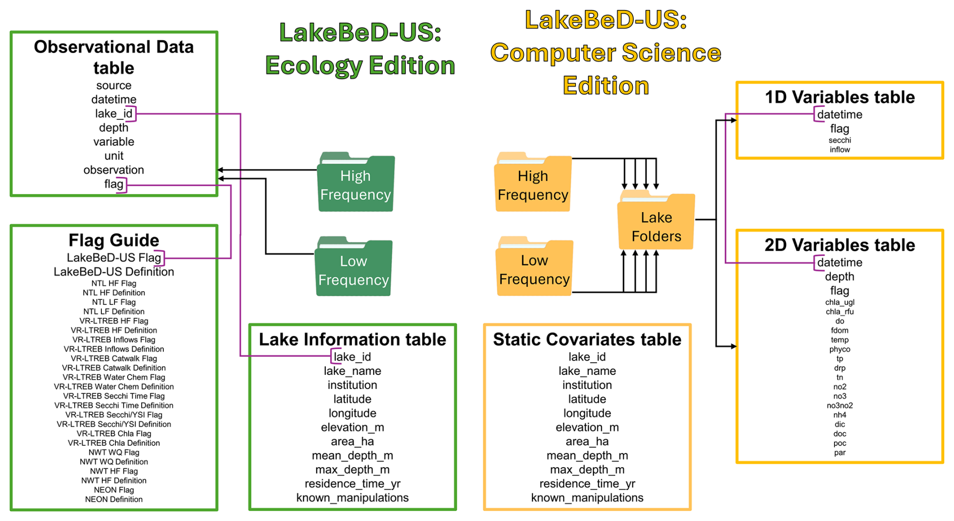
Figure 3 Structure of LakeBeD-US-EE and LakeBeD-US-CSE. Arrows indicate folder contents (e.g., LakeBeD-US-EE contains high- and low-frequency folders that each contain an observational data table). Purple connectors indicate common columns by which to link tables. LakeBeD-US-CSE contains high- and low-frequency folders that each contain separate folders separating data from each lake. Each lake folder contains its own tables with static covariates, 2D variables, and 1D variables.

Ecologists and computer scientists have different analytical approaches and thus different data structures are preferred when working with spatiotemporal data. Ecologists benefit from a long format because this file structure is well suited for aggregated statistics and complex data visualization. The long format also does not require the explicit storage of missing data. Computer scientists, on the other hand, benefit from a wide format due to its compatibility with machine learning workflows. At a high level, machine learning algorithms implemented in popular libraries and frameworks (e.g., NumPy, PyTorch, scikit-learn, and TensorFlow) expect data formatted in the wide format. At a low level, specialized hardware like graphical processing units and tensor processing units, on which these libraries and frameworks are run, are optimized to operate on vector, matrix, and tensor data structures. The wide format lends itself nicely to storage in these formats. Furthermore, wide-format data are often optimized for storage and querying in data systems to enhance computational performance when working with large datasets. Lastly, having all variables in separate columns makes it easier to perform feature selection, engineering, and scaling, which are critical steps in preparing data for machine learning models.

2.3 Assessment and usage of data

To better understand the characteristics of LakeBeD-US, here we showcase the content of LakeBeD-US-EE. Data were loaded into R using the “arrow” package and then queried using “dplyr” (version 1.1.4, Wickham et al., 2023). Visualization made use of the “ggplot2” (version 3.5.1, Wickham, 2016), “ggrepel” (version 0.9.5, Slowikowski, 2024), “gridExtra” (version 2.3, Auguie, 2017), “cowplot” (version 1.1.3, Wilke, 2024), “maps” (version 3.4.2, Becker et al., 2023), and “mapdata” (version 2.3.1, Becker et al., 2022) libraries.

Table 3 Characteristics of lakes included in LakeBeD-US. Location information is presented in Fig. 1.

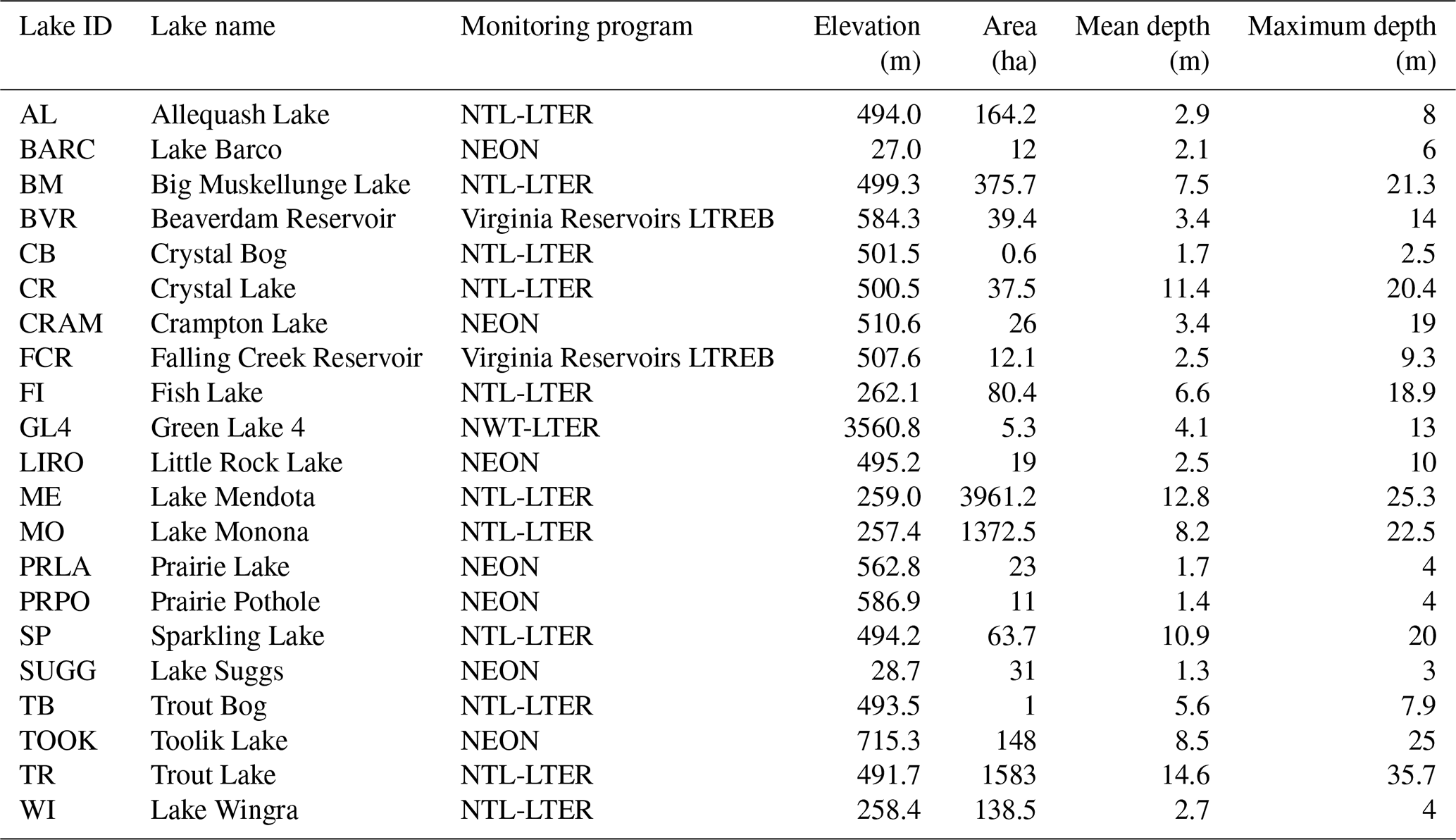
Table 4 Availability of observations by lake in LakeBeD-US-EE. Counts for the number of observations include all depths.

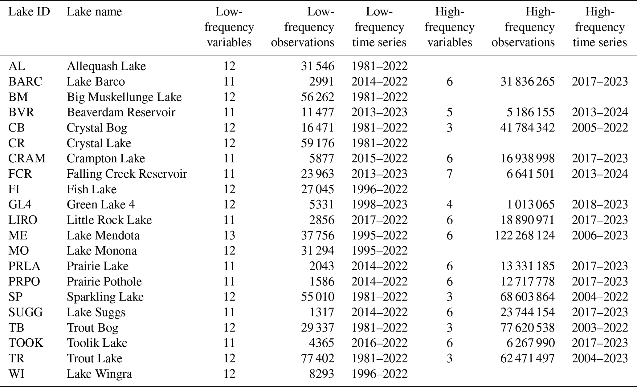
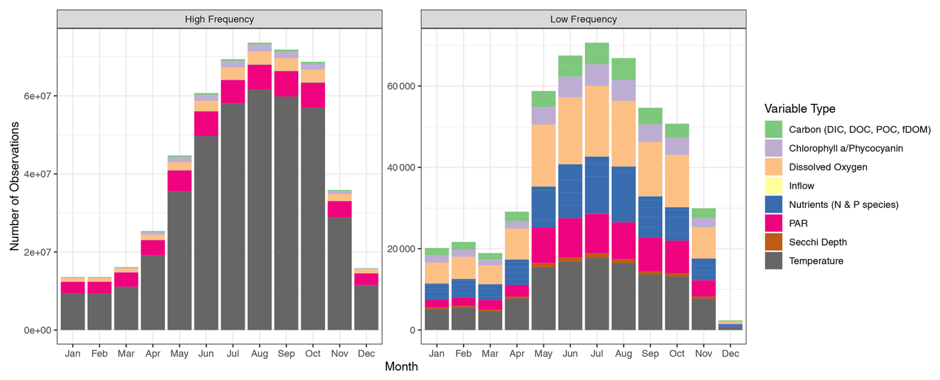
Figure 4 Temporal distribution of observations in LakeBeD-US-EE. Colors represent categories of variables.

3 Ecology Edition: dataset characteristics

3.1 Spatial and temporal extent

While a majority of the lakes included in LakeBeD-US are northern temperate lakes in the state of Wisconsin (Fig. 1), geographic variation is well represented in the dataset alongside other attributes. Toolik Lake is located in the North Slope Borough, Alaska, and is the furthest northwest of any lake in the dataset (Fig. 1), representing an arctic system. In contrast, Lake Suggs and Lake Barco in Putman County, Florida, represent the southeastern-most lakes and are located in a subtropical climate. Suggs and Barco also represent two of the polymictic lakes in the dataset alongside Prairie Lake (Stutsman County, ND), Prairie Pothole (Stutsman County, ND), Lake Wingra (Dane County, WI), and Green Lake 4 (Boulder County, CO) (Preston et al., 2016; Thomas et al., 2023; Lottig and Dugan, 2024). All other lakes in the dataset are dimictic (Gerling et al., 2014; Thomas et al., 2023; Lottig and Dugan, 2024). Green Lake 4 represents the highest-altitude lake in LakeBeD-US, with an elevation of over 3500 m above sea level, a stark contrast to Lakes Suggs and Barco at approximately 27m (United States Geological Survey, 2024). Falling Creek Reservoir and Beaverdam Reservoir are drinking water reservoirs and thus experience a unique set of human manipulations and impacts despite being in a relatively undisturbed forested watershed (Gerling et al., 2014). This provides a potential comparison to the lakes of the NTL-LTER in Wisconsin which have urban and agricultural catchments in the Madison area (Dane County) and relatively undisturbed forested catchments in Vilas County (Magnuson et al., 1997).

Table 5 Number of depths, rounded to 0.5 m, with more than 200 observations measured at a high frequency for each variable in each lake.

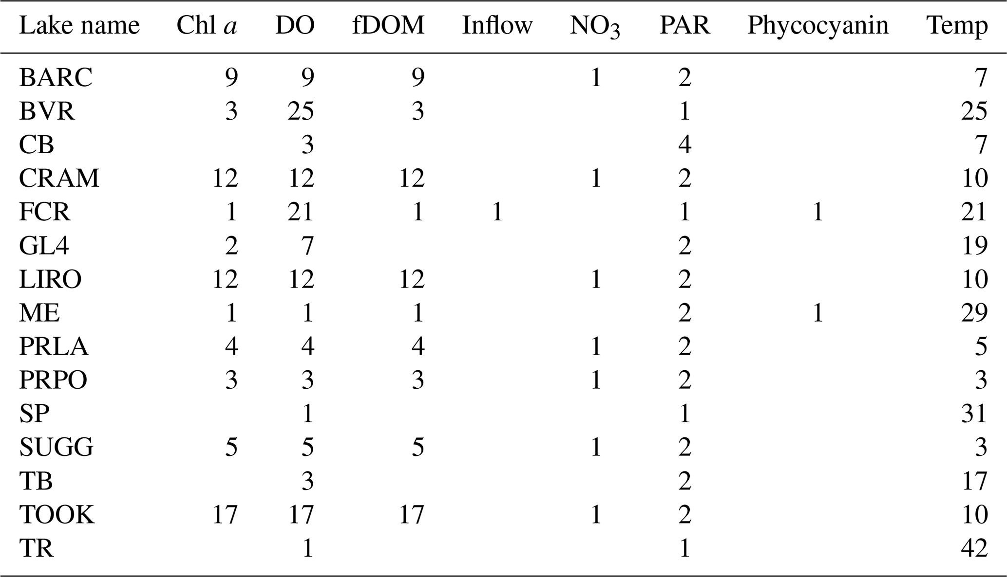
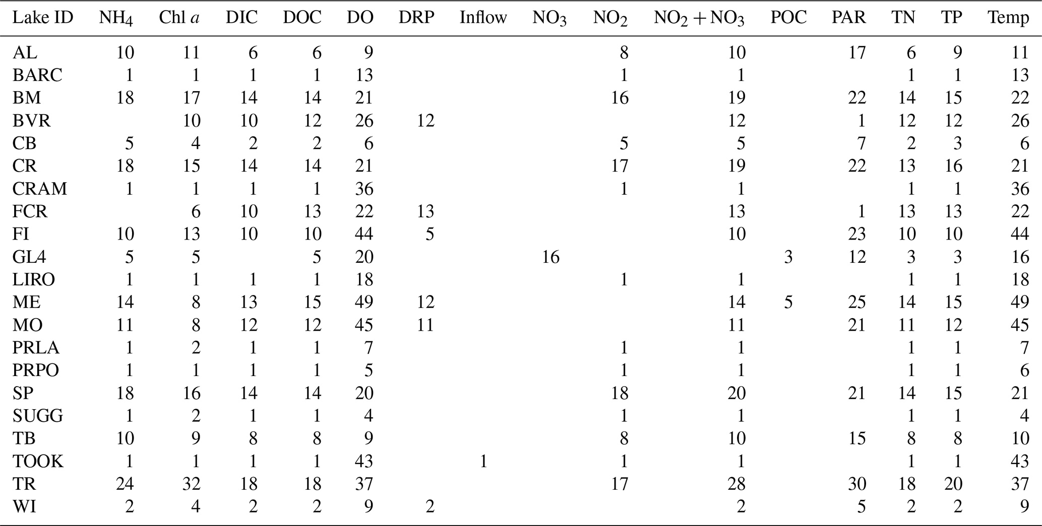
Table 6 Number of depths, rounded to 0.5 m, with more than two observations manually sampled for each variable in each lake. Secchi depth is a 1D variable measured in all lakes that is not shown in this table.

An overview of the temporal characteristics of observational data in LakeBeD-US is given in Table 4 and Fig. 4. The minimum time range of observed values for any lake in the dataset is 5 years, while seven NTL-LTER lakes have over 40 years of data. High-frequency data collection began between 2003 and 2006 for select NTL-LTER lakes, while the majority of high-frequency data collected come from NEON starting in 2017. The Virginia Reservoirs LTREB and NWT-LTER high-frequency sensors were launched in 2013 and 2018, respectively. The longer-running high-frequency programs measure fewer water quality variables (typically temperature, dissolved oxygen, and PAR) relative to the newer programs that have many additional variables including NO₃, fluorescent dissolved organic matter (fDOM), and chlorophyll a. Observations are also not distributed evenly throughout the year. Observations from May through October, half the year during the ice-free season in temperate regions, make up 76.4 % of the total number of observations in the dataset. However, there are observations present during winter months from lakes that do not freeze and from limited under-ice observations (e.g., Lottig, 2022).

The numbers of depths available for each variable in each lake at low and high frequencies are given by Tables 5 and 6. The number of depths sampled and at what intervals they are sampled are highly dependent on the water quality parameter being measured. Among the manually sampled data, variables that can be measured via a sonde cast (e.g., water temperature and dissolved oxygen) are generally captured at a high spatial resolution with intervals of every 0.5 or 1 m depending on the depth of the lake. Variables that are much more expensive or difficult to measure, such as dissolved nutrients, are generally measured at a much lower spatial resolution, sometimes only capturing the surface waters. The spatial resolution of high-frequency measurements varies by the monitoring institution, with some lakes focusing primarily on the surface waters while others capture a greater number of depths.

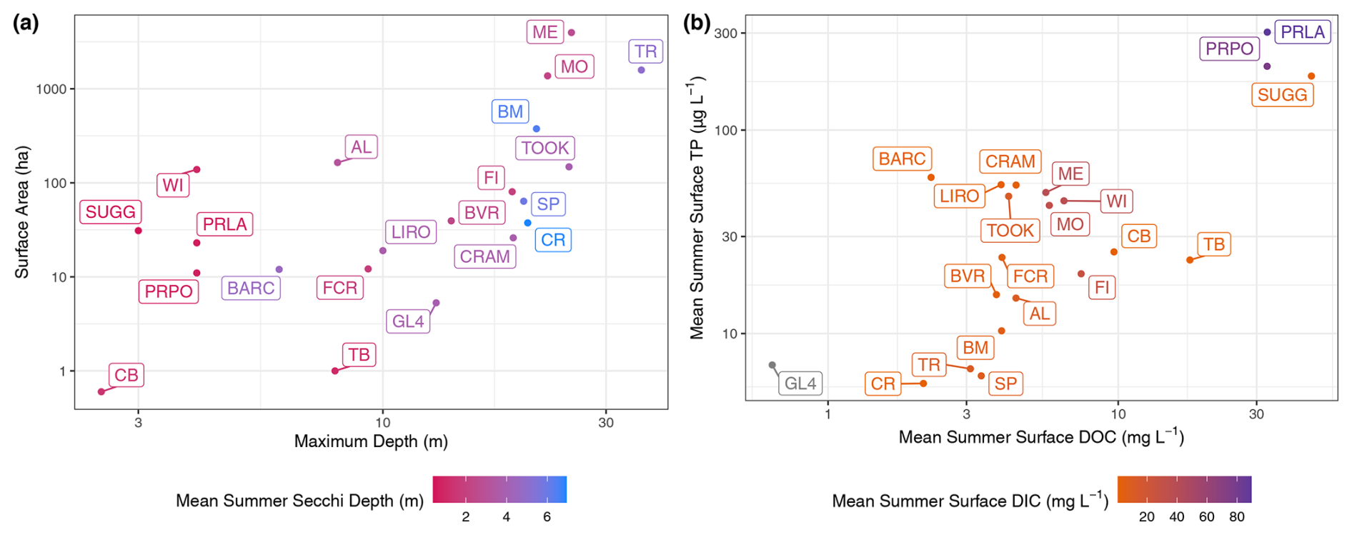
Figure 5 Lakes plotted within gradients of (a) surface area in hectares compared to the maximum depth of the lake in meters. Points and labels are colored according to the mean summertime Secchi depth in meters. (b) Mean summertime surface total phosphorus (TP) concentration in µg L⁻¹ compared to the mean summertime surface dissolved organic carbon (DOC) concentration in mg L⁻¹. Points and labels are colored according to the mean summertime surface concentration of dissolved inorganic carbon (DIC) in mg L⁻¹. Green Lake 4 (GL4) has no observational data for DIC. The surface is defined as the minimum depth sampled for the given time period, which was always within the surface mixed layer of the lake. Summer is defined as the months of June, July, and August.

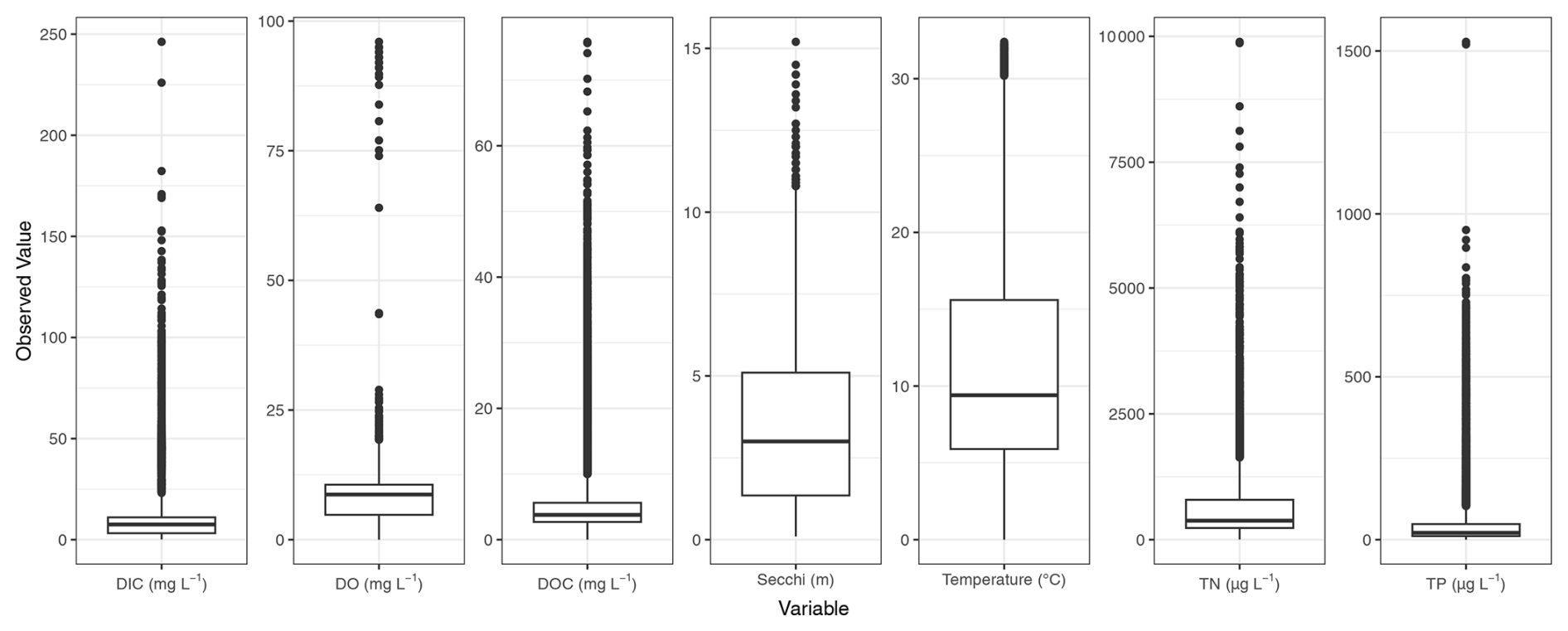
Figure 6 Distributions of observed values for dissolved inorganic carbon (DIC), dissolved oxygen concentration (DO), dissolved organic carbon (DOC), Secchi depth, temperature, total nitrogen concentration (TN), and total phosphorus concentration (TP) across all observations, after quality control, of all lakes in LakeBeD-US-EE.

3.2 Water quality characteristics

The distributions of select lake attributes and water quality variables are given in Figs. 5 and 6. A wide range of lakes are present in LakeBeD-US in terms of surface area, depth, and indicators of trophic status. It is of note that water quality variables often follow a non-normal distribution (Helsel, 1987; Lim and Surbeck, 2011), and LakeBeD-US is no exception (Fig. 6). This skewness is characteristic of environmental data and should be considered by users of the dataset.

4 Benchmark task

4.1 Computer Science Edition benchmark

In this section, we develop a machine learning model to predict the daily median dissolved oxygen concentration (do) and water temperature (temp) in Lake Mendota to showcase the utility and applicability of LakeBeD-US-CSE for the machine learning task of multivariate time series prediction.

4.1.1 Data selection

LakeBeD-US-CSE provides two datasets for Lake Mendota: low-frequency and high-frequency datasets. Both temporal frequencies were considered in this benchmark. Observations from the low- and high-frequency datasets with the flag codes indicated in Table 2 were selected for use in the benchmarking task.

While LakeBeD-US features data from across many discrete depths through time, we considered data across a single depth of Lake Mendota to simplify the benchmark. This required considering the percentage of missing values at each depth that the low- and high-frequency datasets reported. With the exception of water temperature, all high-frequency variables were measured only at a depth of 1 m. Similarly, the low-frequency data reported large percentages (> 85 %–90 %) of missing values for all variables across all depths. Among all variables reported in the datasets, we selected chlorophyll a (chla_rfu), photosynthetic active radiation (par), and phycocyanin (phyco) from the datasets to be used as covariates due to the high number of observations present for these variables in the high-frequency data.

4.1.2 Data wrangling

The following steps were taken to prepare the data for modeling.

• 1.

  Timescale standardization. The timescales of the low- and high-frequency datasets were discontinuous, containing large multi-day gaps in the time series. We created two uniform time series with no discontinuities at the resolution that was permitted by each dataset: daily resolution for the low-frequency data and minutely resolution for the high-frequency data from the earliest to the most recent dates and times in both datasets. The new low-frequency dataset's timescale spanned 9 May 1995 to 1 November 2022, while the new high-frequency dataset's timescale spanned 28 June 2006 at 02:31:00 LT to 19 November 2023 at 15:26:00 LT. This step was critical to providing a more accurate value for the percentage of missing data.

• 2.

  Data harmonization. To mitigate the issue of high percentages of missing observations, the low- and high-frequency datasets were merged into a single dataset. Since the low-frequency dataset begins in 1995, as opposed to the high-frequency dataset which begins in 2006, the resulting harmonized dataset had an even larger percentage of missing values. From this merged dataset, we selected only the observations recorded since the start of the high-frequency dataset to minimize the amount of imputation that would be required.

• 3.

  Downsampling and aggregation. The harmonized dataset was downsampled to a daily resolution by calculating the median value within each day.

• 4.

  Splitting and sliding window sampling. The data were split 80 %–10 %–10 % chronologically into a training–validation–testing split. The training split was standardized (Z-score-normalized) and the standardization parameters were applied to the validation and testing splits. After standardization, windowed samples were generated for each split. 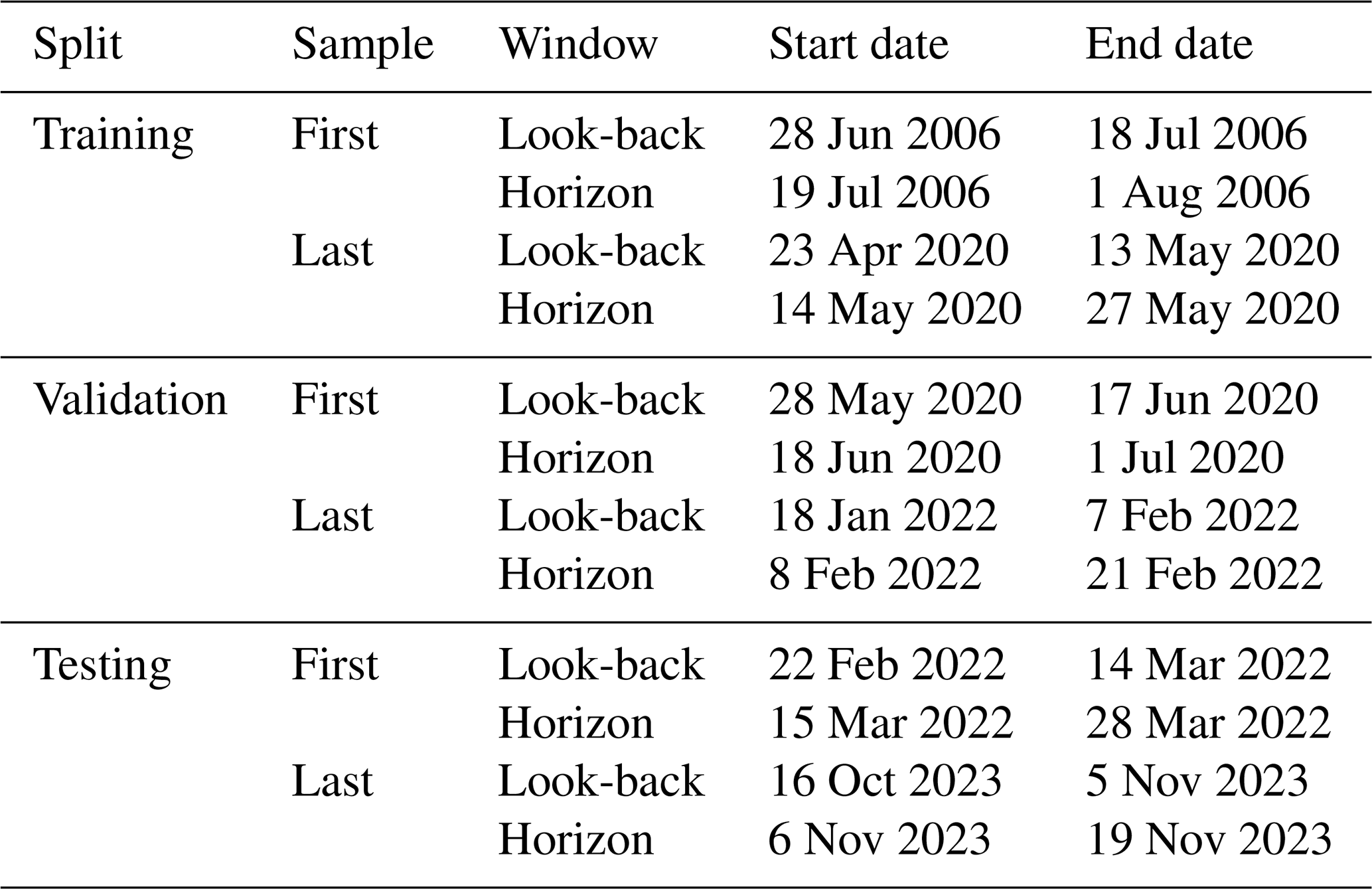A windowed sample consists of 21 d of observations of all features (chla_rfu, par, phyco, do, temp) as inputs, referred to as a “look-back window”, and the subsequent 14 d of do and temp as targets, referred to as a “horizon window”. For example, if we considered the observations of all features from 1 to 21 January to be the look-back window, the do and temp observations from 22 January to 4 February would be the horizon window. The subsequent sample would be formed by “sliding the (look-back and horizon) window” by 1 d into the future (i.e., the second sample's look-back window would span 2 to 22 January and the horizon window would span 23 January to 5 February). The sampling was carried out such that the horizon window of the last sample would not extend farther than the end of each respective split to avoid data leakage between splits. The start and end dates of the look-back and horizon window of the first and last sample in each split are given in Table 7.

Table 7 Start and end dates of each look-back and horizon window for the first and last samples in each split.

• 5.

  Imputation. Prior to windowed sampling, the percentages of missing values for each split were calculated. These values are listed in Table 8.

  The missing values in the input look-back windows for each split were imputed using the self-attention-based imputation for time series (SAITS) method (Du et al., 2023). Traditional imputation techniques, such as spline interpolation and k-nearest neighbors, often rely on assumptions about simple relationships between adjacent data points. In contrast, SAITS leverages a self-attention mechanism to identify and emphasize relevant information across the entire dataset, even when pertinent data points are temporally distant. This approach allows SAITS to effectively capture complex temporal patterns and inter-variable relationships. During training, SAITS introduces artificial missing values into the dataset and attempts to impute them. By minimizing the discrepancy between its imputations and the original values, SAITS learns to accurately reconstruct missing data, resulting in more reliable and comprehensive datasets for analysis.

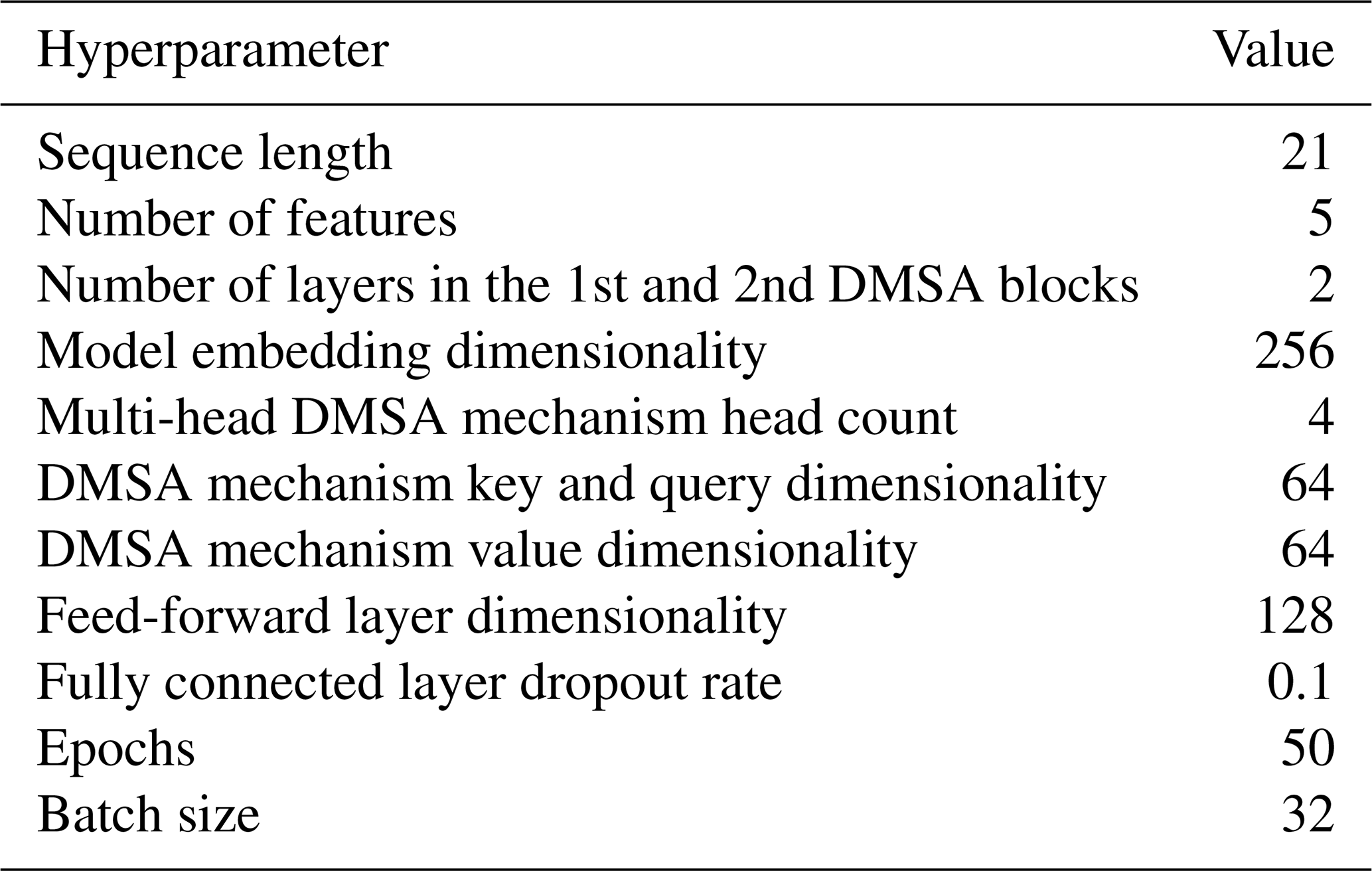
  A SAITS model was trained on the windowed samples from the training split using the hyperparameters specified in Table 9 and applied on the input look-back windows of the training, validation, and testing splits. Since no ground truth for the dataset was present, the quality of the imputation could not be empirically measured and instead was inferred through the predictive skill of the model. The target horizon windows were not imputed because it would have been difficult to identify if strong performance of the model was a result of a good model or an overly simplistic imputation (e.g., a simple horizontal line).

Table 8 Percentage of missing values per variable in each split.

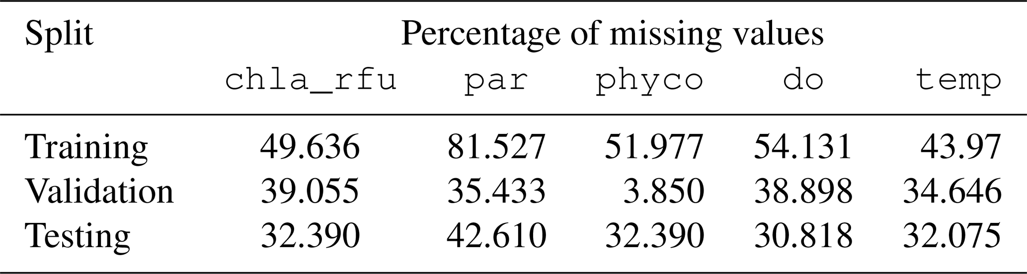
Table 9 SAITS imputation model hyperparameters. Diagonally masked self-attention (DMSA) is a component of SAITS.

4.1.3 Modeling

The components of the modeling process used for our benchmark are outlined below. All modeling was conducted using PyTorch (Paszke et al., 2019).

• Model architecture. A sequence-to-sequence (seq2seq) long short-term memory recurrent neural network (LSTM-RNN) was constructed to predict dissolved oxygen concentration and water temperature. Seq2seq modeling arose from the field of natural language processing, specifically neural machine translation (NMT; Cho et al., 2014; Sutskever et al., 2014). In NMT, given an input sentence in one language, we wish to translate the sentence to another language using a neural network such that the translation has semantic meaning and obeys the syntax of the target language. Observations in a time series, like words in a sentence, have an inherent temporal ordering. Thus, the problem of time series prediction conveniently lends itself to this modeling paradigm.

  A seq2seq model follows an autoencoder architecture, comprising two main components: an encoder and a decoder. The encoder is built on an LSTM-RNN. It processes the input data in a sequential manner, mapping the input to a high-dimensional vector, called a “hidden state”, at each time step of the input. This hidden state exists in a latent feature space (also referred to as embedding space), which can abstractly be thought of as a summary of the input sequence up to that moment in time. When the encoder has encoded the final time step of the input sequence into a hidden state, the final hidden state vector contains a summary of the entire input time series. This final hidden state is referred to as a “context vector” that encapsulates the critical information of the sequence in a compressed form. The decoder, another LSTM-RNN, uses this context vector as a foundation to generate the desired target sequence. Operating in an autoregressive manner, the decoder predicts each time step in the future sequence, feeding each prediction back as input to inform the next. This autoregressive process continues until the full sequence in the prediction window is generated.

• Training strategy

  • Cost function. The parameters of the model were trained by minimizing the root mean square error (RMSE) between the predicted target horizon window and the observed horizon window. Since the target horizon windows in each sample were not imputed, a masked loss computation was employed. In situations where the observed horizon window contained missing observations, the error was only computed between observations that were jointly present in the prediction and the observed horizon window. If the horizon window contained no observations, then the sample was omitted from the error computation. The RMSE cost function was minimized using the adaptive moment estimation (AdaM) optimizer and a “reduce learning rate on plateau” learning rate scheduler. Learning rate scheduling is a technique to adaptively adjust the learning rate during training based on the model's performance on the validation split. The core idea is to reduce the learning rate when progress stalls, helping the model to escape saddle points or local minima in the cost landscape, thereby potentially achieving a better final result.

  • Regularization. We leveraged early stopping and weight decay regularization. Early stopping is a regularization technique that mitigates overfitting of the model by monitoring the performance on the validation split. If the validation cost starts to increase over time, the model halts the training process. Weight decay is a regularization technique that operates by subtracting a fraction of the previous weights when updating the weights during training, effectively making the weights smaller over time. This subtraction of a portion of the existing weights ensures that during each iteration of training, the model's parameters are nudged towards smaller values.

• Hyperparameter selection. Model architecture and learning hyperparameters were optimally chosen using the “tree-structured Parzen estimator” algorithm in the Optuna library by minimizing the validation cost over 50 trials (Akiba et al., 2019). The final hyperparameters are given in Table 10.

Table 10 Final model architecture and learning hyperparameters.

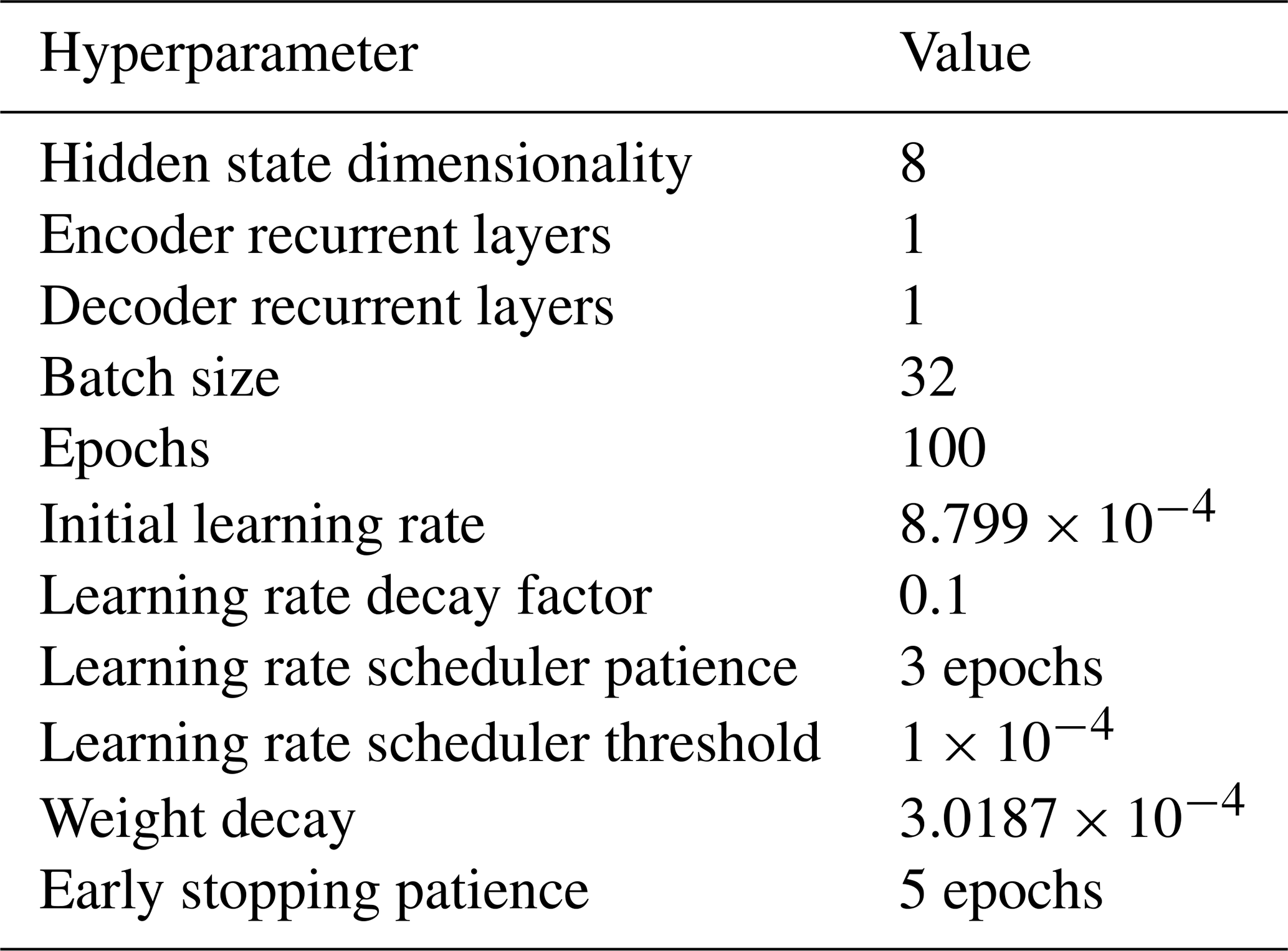
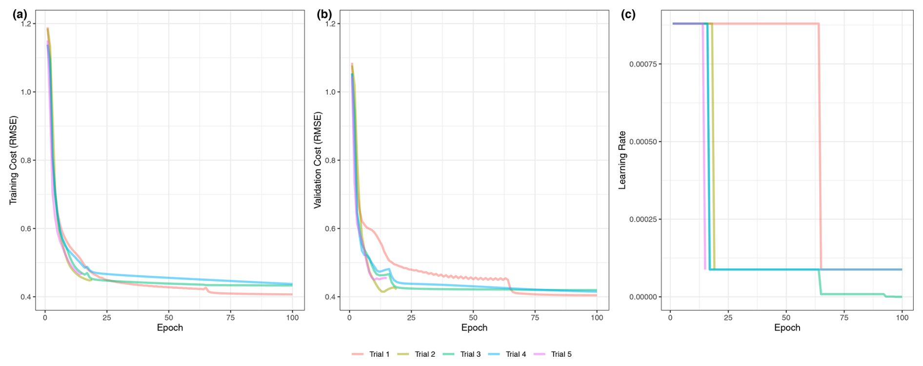
Figure 7 Training cost, validation cost, and learning rate of the machine learning benchmark. The cost, a measure of model error, for the training (a) and validation (b) splits is shown as a function of the number of epochs. The learning rate, or amount of change between iterations of the model in response to error, is shown (c). Five trials are shown in different colors.

4.1.4 Results

The learning curve shown in Fig. 7a shows the performance of the model on the training and validation splits at each epoch in the training process, while the learning rate schedule in Fig. 7b shows the reduction in the learning rate of the model until convergence. The final standardized RMSE of the model on each data split is presented in Table 11.

Table 11 Model performance on each data split as measured with standardized RMSE across five trials.

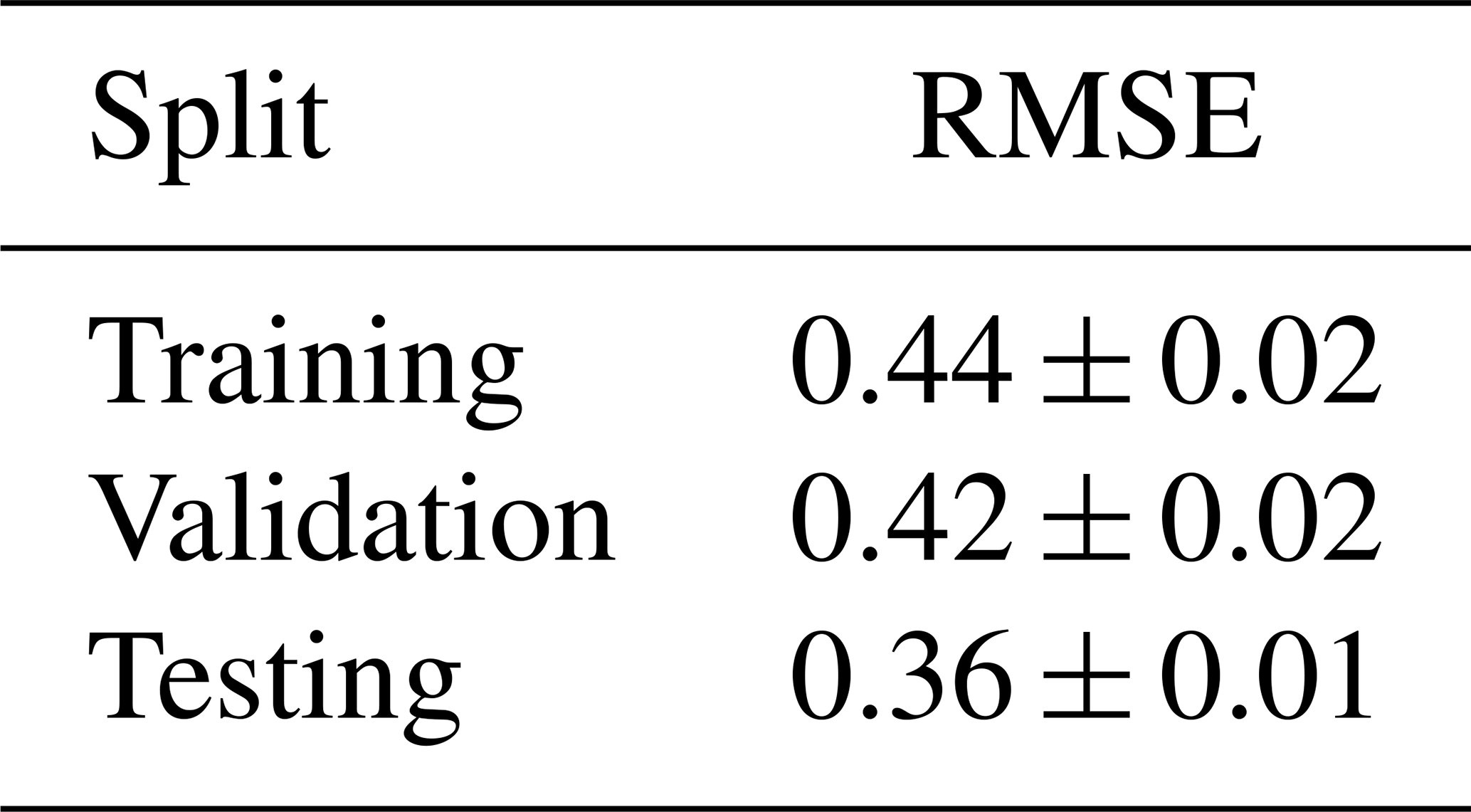
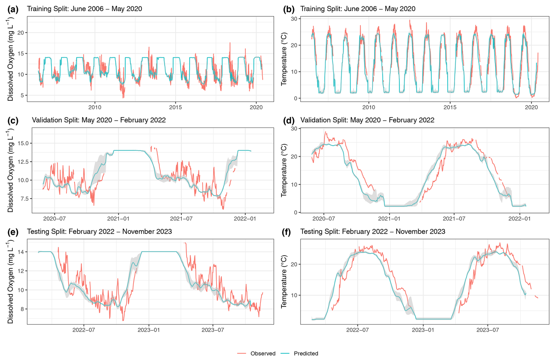
Figure 8 Machine learning model predictions of surface water dissolved oxygen and temperature. Observed (red) and predicted (blue) dissolved oxygen (a, c, e) and temperature (b, d, f) are shown. Training (a, b), validation (c, d), and testing (e, f) splits are shown. The gray-shaded areas represent the confidence intervals.

The predictions for dissolved oxygen concentration and water temperature for the training, validation, and testing splits are shown in Fig. 8. For a given split, after the 21st day in the window, a 14 d ahead series of predictions is generated on each day. This results in multiple, potentially up to 14, overlapping predictions for a single day. We consolidated these overlapping predictions by calculating the median predicted value for each day across all predictions. This yields a single, continuous series of predictions for an entire split's timeline. The predictions shown in Fig. 8 were obtained by continuous predictions from each trial in each split. The confidence interval was generated by taking the minimum and maximum values for each date and time across each continuous series of predictions. Table 12 shows the unstandardized RMSE between the continuous predictions from each trial and the observed dissolved oxygen concentration and water temperature across the entire time series within each split.

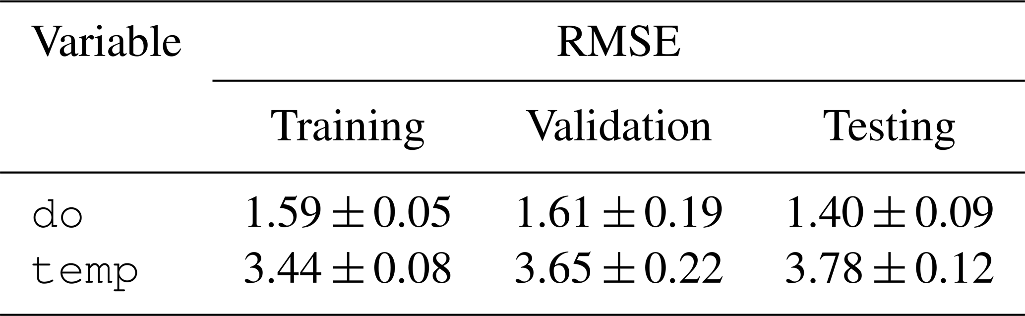
Table 12 Mean masked unstandardized RMSE and standard deviation between the continuous time series predictions and observed values for each split across all trials. Dissolved oxygen (do) is reported in mg L⁻¹ and water temperature (temp) is reported in degrees Celsius.

4.1.5 Benchmark task discussion

With our benchmark task, we showcase the applicability of LakeBeD-US to multivariate time series prediction of two water quality variables. Our machine learning model performed comparably to existing process-based models for the purpose of predicting the dissolved oxygen concentration. In predicting the dissolved oxygen concentration of the surface of Lake Mendota, an iteration of the GLM-AED2 model (Hipsey et al., 2019) calibrated by Ladwig et al. (2021) reported an RMSE of 2.77 mg L⁻¹ and a model constructed by Hanson et al. (2023) reported an RMSE of 1.45 mg L⁻¹. Our model predicted dissolved oxygen in the testing dataset with an RMSE of 1.40 mg L⁻¹ (Table 12), which is comparable to the aforementioned process-based water quality models. When predicting temperature our model did not perform as well as the process-based models that reported RMSE values of around 1.30 °C, which is less than half of our machine learning model's error (Table 12). While the predictions generated by our model have room for improvement, they show that LakeBeD-US-CSE can be used to create water quality models with machine learning. Water temperature in particular is a variable that has been shown to be a useful tool for comparison of model performance in ecological tasks (Read et al., 2019).

5 Discussion

In this paper, we introduce LakeBeD-US: a dataset designed to foster the advancement of machine learning technologies in ecological applications. By combining spatially and temporally extensive datasets, we offer a dataset that can be used in benchmarking tasks that address the scales of variability in the drivers of lake water quality. LakeBeD-US is compatible with ecological analysis, novel computer science methodologies, or both through the interdisciplinary paradigm of KGML.

5.1 Limitations and considerations for use of LakeBeD-US

LakeBeD-US is not a representative sample of the water quality gradients found in lakes of the world (Verpoorter et al., 2014; Messager et al., 2016), but it is representative of water quality data that are available. Limnological sampling efforts tend to favor large, easily accessible lakes that are used more frequently for their natural resources, and most samples are taken during the ice-free season (Stanley et al., 2019). A majority of the observations in LakeBeD-US represent the ice-free season (Fig. 4), and 13 of the 21 lakes included in the dataset are located within the state of Wisconsin (Fig. 1), with the most well-observed lake being the large, eutrophic, and heavily utilized Lake Mendota (Table 4). Despite this, LakeBeD-US still captures a variety of lake characteristics and geographic locations that enable users to investigate those attributes' relationship with water quality dynamics (Fig. 5).

LakeBeD-US does not account for methodological or equipment differences among its datasets. Sensors and laboratory procedures change over time and between monitoring institutions, which is information not present in LakeBeD-US but present in the source datasets (listed in Sect. S1 in the Supplement). The harmonization procedure of LakeBeD-US assumes the accuracy and precision of the observed value of the source data, excepting any quality flags that have been applied to the data. Potential methodological differences should be investigated when encountering any unexplained changes in water quality trends present in LakeBeD-US, particularly with data that use RFU.

The observed water quality variables exhibit a heavy skewness that is common among of data of this kind (Fig. 6; Helsel, 1987; Lim and Surbeck, 2011). Considerations should be taken when analyzing or using these data to limit the effect of this skewness, as omitting flagged values or outliers may not be enough (Virro et al., 2021). Transformations may need to be applied to the data before use, such as the standardization applied in the benchmark task of this paper.

Unlike many benchmark datasets, LakeBeD-US contains numerous missing values. This is a problem typical of environmental data. Fortunately, the handling of missing values in environmental data by machine learning algorithms is an active area of research (Rodríguez et al., 2021), and LakeBeD-US can act as a testing ground for developing novel methods.

5.2 LakeBeD-US for ecological applications

The LakeBeD-US dataset has numerous applications for studying lake water quality. Previous studies using its source data have provided insights into many of the drivers and dynamics of water quality (e.g., Hanson et al., 2006; Ladwig et al., 2021; Thomas et al., 2023). The cross-region synthesis of LakeBeD-US offers new opportunities to further advance our understanding of these dynamics. For instance, high-frequency data can be used to assess the impact of pulse disturbances, such as heatwaves or storms, on water quality across geographic or trophic gradients. Similarly, high-frequency chlorophyll data can offer insights into the prevalence of algal blooms in different regions. The long-term monitoring data within LakeBeD-US are essential for examining changes in trophic state across decades. These insights can emerge from both direct data analysis and the development of lake water quality models.

5.3 LakeBeD-US as a machine learning benchmark

The benchmarking task in Sect. 4 is a straightforward example of how machine learning can be applied to lake water quality prediction using LakeBeD-US-CSE. The machine learning model performed comparably to many existing process-based models when predicting dissolved oxygen concentration and temperature in Lake Mendota's surface waters (Sect. 4.1.5; Hanson et al., 2023; Ladwig et al., 2021). This showcases the applicability of machine learning to ecological problems, and the error in the model showcases the utility of LakeBeD-US as a benchmark dataset. Machine learning algorithms other than the LSTM-RNN used here may have a different performance for this task, an understanding of which is a vital part of the model selection process in ecological studies. The variety of lakes in LakeBeD-US enables future studies to investigate the performance of machine learning, mechanistic, and hybrid knowledge-guided machine learning models when making predictions across multiple lakes, trophic statuses, or temporal frequencies.

LakeBeD-US was assembled as part of an effort to advance the science of knowledge-guided machine learning (KGML) in ecological applications. There are many potential uses of the dataset for investigating water quality dynamics using these techniques. Transfer learning is the use of a machine learning model trained on a number of source tasks applied to a new target task with limited data (Karpatne et al., 2024), which is a method that has been applied to lakes (Willard et al., 2021). LakeBeD-US features a varied selection of lakes, making it suitable for the application of transfer learning methods for lake systems. Building upon this idea of transfer learning, there has been recent advancement in the application of foundation models to environmental data, which can be pre-trained on a broad, heterogeneous dataset and then fine-tuned on a more specific dataset to a given task (Lacoste et al., 2023; Nguyen et al., 2023; Karpatne et al., 2024). LakeBeD-US may prove useful in the application of foundation models or other KGML methods (e.g., modular compositional learning; Ladwig et al., 2024) to water quality.

5.4 Potential for the expansion of LakeBeD-US

While the number of lakes in LakeBeD-US is modest relative to national- or global-scale studies (e.g., Soranno et al., 2017; Solomon et al., 2013), the frequency and duration of its data provide unique opportunities for expanding scientific understanding of aquatic ecosystem dynamics. Ensuring that long-term water quality datasets meet the rigorous requirements for LakeBeD-US requires working with the scientists and organizations who collect the data. This will have the added benefit of involving more lake ecologists in water quality modeling endeavors (Hanson et al., 2016). The Global Lake Ecological Observatory Network (GLEON) is an example of this type of community involvement in data collection, harmonization, and analysis (Weathers et al., 2013; Hamilton et al., 2015).

Updates to include more data, more lakes, and more water quality variables are possible and collaboration in the creation of new additions to LakeBeD-US is encouraged. The data provenance and versioning tools of the Environmental Data Initiative and Hugging Face repositories make it possible for specific versions of both LakeBeD-US-EE and LakeBeD-US-CSE to be referenced in future studies. The source code to harmonize LakeBeD-US-EE searches the source repository for the latest release of the source data, enabling new updates to the existing sources to be integrated seamlessly, as long as major format changes in the source data do not occur. Adding new data sources to LakeBeD-US-EE is possible, requiring that a new R script to download and harmonize the observational data be written and the Data_Controller.R and Lake_Info.R files in the source code updated accordingly. LakeBeD-US-EE's use of the Parquet format allows for additions to the dataset without having to rewrite the entirety of the dataset's files. LakeBeD-US-CSE is created dynamically based on the content of LakeBeD-US-EE, allowing for parity between the two versions. Stewards of long-term water quality monitoring data are encouraged to become contributors to LakeBeD-US through the creation of modular additions to the Parquet dataset. These modules would emulate the design of LakeBeD-US-EE, namely the R scripts to format the data and write them to Parquet files, meaning that users of the data could seamlessly add the contents of any community-made module to the base LakeBeD-US-EE data. There would then be potential for integration of the data modules into the base LakeBeD-US in future revisions if that collaboration is desired.

6 Data availability

LakeBeD-US: Ecology Edition is available in the Environmental Data Initiative repository (https://doi.org/10.6073/pasta/c56a204a65483790f6277de4896d7140; McAfee et al., 2024). LakeBeD-US: Computer Science Edition is available in the Hugging Face repository (https://doi.org/10.57967/hf/3771; Pradhan et al., 2024).

7 Conclusions

LakeBeD-US is a dataset of lake water quality observations combining high- and low-frequency observations from 21 lakes across the United States collected by different monitoring institutions for the intention of AI benchmarking. This dataset is one of the first of its kind to capture water quality at a high spatial and temporal resolution in the selected lakes and be available in formats conducive to both ecological analyses and novel computer and data science approaches. As a benchmark dataset, LakeBeD-US was designed to be used to advance the science of knowledge-guided machine learning and foster collaboration between ecologists and computer scientists.

There are many planned and potential uses for LakeBeD-US. As a benchmark dataset designed with machine learning in mind, LakeBeD-US offers an opportunity to test and compare new machine learning methodologies in an ecological context. Aspects of LakeBeD-US such as data skewness and missing values are prevalent in environmental data and this dataset offers opportunities for the scientific community to investigate methods for mitigating these issues for machine learning models. This collection of data is also valuable for the investigation of water quality dynamics using statistical or mechanistic models. These advances in water quality modeling, prediction, and forecasting are vital in creating a greater understanding of aquatic systems and informing more thoughtful utilization of aquatic resources.

Appendix A: Table and variable metadata

Table A1 LakeBeD-US: Ecology Edition lake information table metadata.

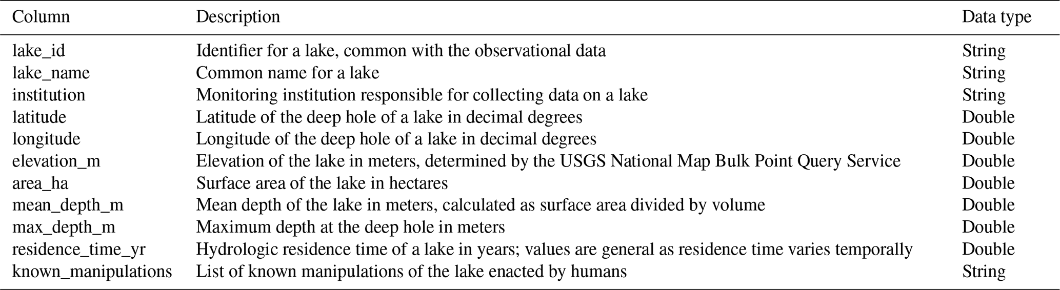
Table A2 LakeBeD-US: Ecology Edition high- and low-frequency observation table metadata.

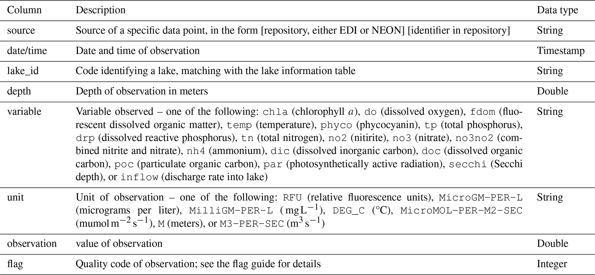
Table A3 LakeBeD-US: Ecology Edition flag guide table metadata. Citations for source datasets can be found in Sect. S1 in the Supplement. Each row of the flag guide table corresponds to a definition, where common definitions between flags of data sources are aligned.

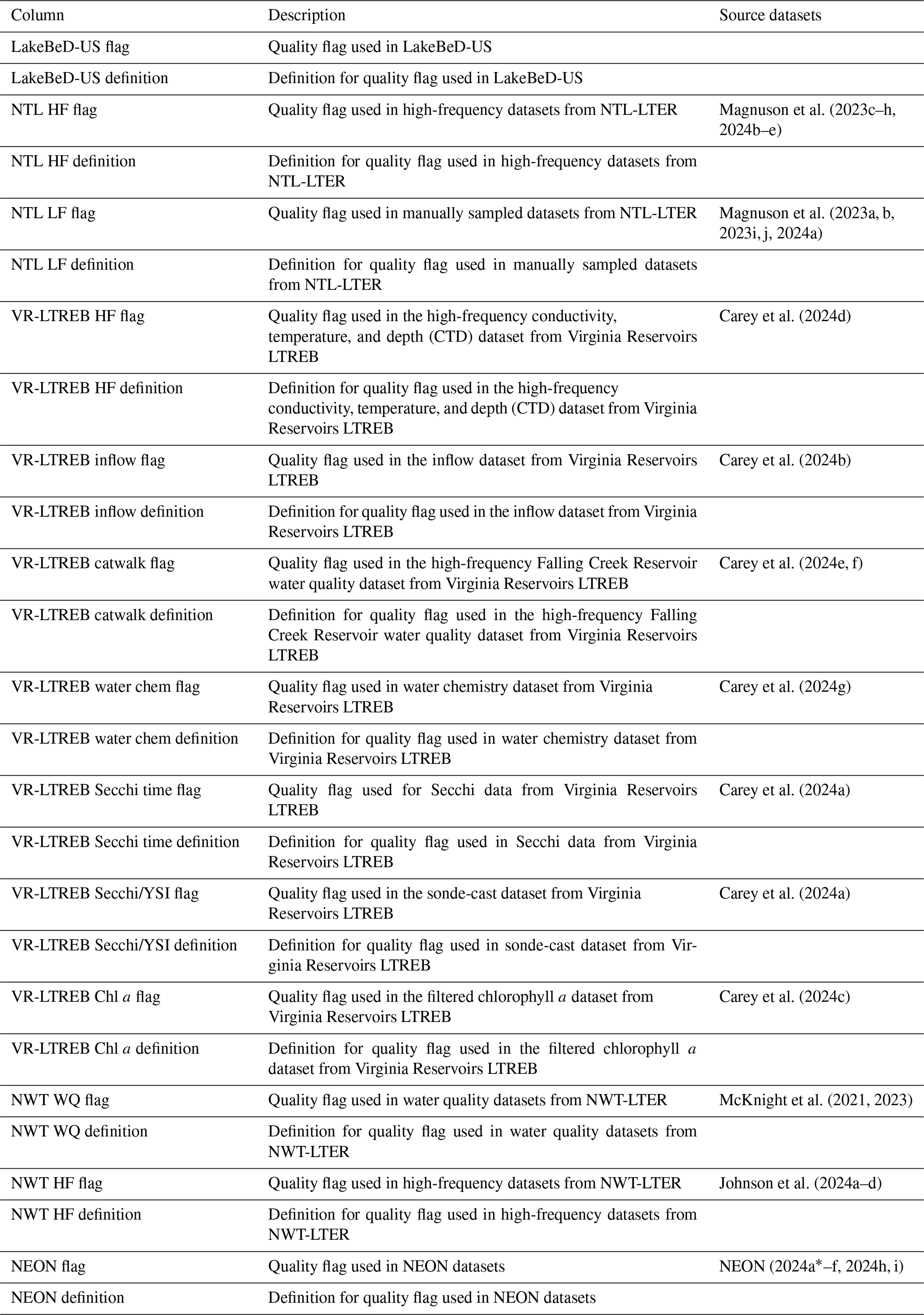
^∗ LakeBeD-US lists the maximum depth of a lake for Secchi depth when the Secchi depth hits the bottom. Secchi data from NEON (2024a) list when the disk hits the lake bottom and the maximum depth measured but reports a missing value for Secchi when this happens. In these cases, LakeBeD-US lists the maximum depth as the Secchi depth and applies a flag indicating this substitution was made. This flag does not originate from NEON (2024a).

Table A4 Metadata for LakeBeD-US: Computer Science Edition. All possible columns from the high- and low-frequency datasets and 1D and 2D variables are listed.