A revised and expanded deep radiostratigraphy of the Greenland Ice Sheet from airborne radar sounding surveys between 1993 and 2019

Between 1993 and 2019, NASA and NSF sponsored 26 separate airborne campaigns that surveyed the thickness and radiostratigraphy of the Greenland Ice Sheet using successive generations of coherent VHF radar sounders developed and operated by The University of Kansas. Most of the ice sheet's internal VHF radiostratigraphy is composed of isochronal reflections that record its integrated response to past centennial- to multi-millennial-scale climatic and dynamic events. We previously generated the first comprehensive dated radiostratigraphy of the Greenland Ice Sheet using the first 20 of these campaigns (1993–2013) and investigated its value for constraining the ice sheet's history and modern boundary conditions. Here we describe the second version of this radiostratigraphic dataset using all 26 campaigns, which includes substantial improvements in survey coverage and was mostly acquired with higher-fidelity systems. We improved quality control and accelerated reflection tracing and matching by including an automatic test for stratigraphic conformability, a thickness-normalized reprojection for radargrams, and automatic inter-segment reflection matching. We reviewed and augmented the 1993–2013 radiostratigraphy, and we applied an existing independently developed method for predicting radiostratigraphy to the previously untraced campaigns (2014–2019) to accelerate their semi-automatic tracing. The result is a more robust radiostratigraphy and age structure of the ice sheet that covers up to 65 % of the ice sheet and includes > 58 600 km of newly traced reflections from the 2014–2019 campaigns. This dataset can be used to validate the sensitivity of ice-sheet models to past major climate changes and constrain long-term boundary conditions (e.g., accumulation rate). Based on these results, we make several recommendations for how radiostratigraphy may be traced more efficiently and reliably in the future. This dataset is freely available at https://doi.org/10.5281/zenodo.14182641 (MacGregor et al., 2025). It includes all traced reflections at the spatial resolution of the radargrams and grids (5 km horizontal resolution) of the depths of isochrones between 3 and 115 ka and ages between 10 % and 80 % of the ice thickness; associated codes are available at https://doi.org/10.5281/zenodo.14183061 (MacGregor, 2024a).

1 Introduction

The Greenland Ice Sheet (GrIS) is losing mass rapidly and is projected to do so for the foreseeable future unless substantial mitigation of anthropogenic warming is undertaken (Aschwanden et al., 2019; Goelzer et al., 2020; Otosaka et al., 2023). Ice-sheet models are the essential tools used to make these projections, but the uncertainty in these projections is large and significantly affects how society might respond to the global and regional sea-level change caused by GrIS wastage (Aschwanden et al., 2021). Numerous efforts are underway to reduce this uncertainty (e.g., Aschwanden and Brinkerhoff, 2022), and among the major challenges that these efforts seek to address are the initialization of these models prior to applying projected external forcings (typically atmospheric and oceanic) and whether their long-term sensitivity to anthropogenic climate change is consistent with that inferred from paleoclimatic records (e.g., Goelzer et al., 2018; Briner et al., 2020). Fortunately, the GrIS contains within itself a substantial and spatially well-distributed archive of its integrated response to past climate change: its isochronal radiostratigraphy. Further, this radiostratigraphy can constrain the subsurface state and dynamics of the present-day GrIS in a manner not achieved by other spatially distributed observations; it is also potentially valuable for identifying well-initialized instances of ice-sheet models (e.g., Bingham et al., 2024).

MacGregor et al. (2015a; hereafter M15) generated the first large-scale dated radiostratigraphy of the GrIS. That study was made possible by the abundance of high-quality very high frequency (VHF) airborne radar sounding data collected in the prior two decades (1993–2013, all years CE) sponsored by the United States (US) National Aeronautics and Space Administration (NASA) and National Science Foundation (NSF; CReSIS, 2024), advances in radar sounder design led by The University of Kansas (KU; e.g., Gogineni et al., 1998) and its Center for Remote Sensing and Integrated Systems (CReSIS; e.g., Rodríguez-Morales et al., 2014; Arnold et al., 2019), and a suite of synchronized deep ice cores collected by international consortiums led primarily by Denmark and the United States (e.g., Rasmussen et al., 2006; Dahl-Jensen et al., 2013; Seierstad et al., 2014; Mojtabavi et al., 2020). M15 introduced several advances in prediction, mapping, dating, validation, and gridding of radiostratigraphy to generate the first ice-sheet-wide age volume for either of Earth's two remaining ice sheets. That study enabled numerous improvements in mapping of key ice-sheet boundary conditions (e.g., MacGregor et al., 2015b, 2016a, b, 2022; Dow et al., 2018). It also motivated refinements to – and assessment of – methods for mapping and modeling radiostratigraphy (e.g., Born, 2017; Xiong et al., 2018; Delf et al., 2020; Born and Robinson, 2021). However, no subsequent study has significantly improved upon the M15 dataset itself, either by infilling isochronal reflections that were unmapped by M15 or by incorporating the large quantity of additional similar airborne radar sounding data collected as part of NASA's Operation IceBridge (OIB) in 2014–2019 that was not included in M15 (MacGregor et al., 2021).

Here we describe version 2 (v2) of the GrIS radiostratigraphy dataset and the methods to generate it, with a particular emphasis on methodological improvements introduced since M15 and remaining uncertainties. Based on the development of this dataset, we identify future opportunities for developing a more complete deep radiostratigraphy of the GrIS and make recommendations for future improvements in tracing methods.

2 Airborne radar sounding data

To build this second version of the GrIS-wide radiostratigraphy, we first evaluate the same 1993–2013 VHF radar sounding data collected over the GrIS by KU/CReSIS as M15 used to generate v1 (Table 1; Fig. 1; CReSIS, 2024). We further consider the additional six OIB campaigns of VHF radar sounding data collected annually during boreal springtime between 2014 and 2019 by KU/CReSIS using identical or similar system configurations. These data were recorded coherently and subsequently focused using synthetic aperture radar (SAR) methods by KU/CReSIS. The nominal vertical resolution of these processed data is 2.5–4.4 m, which is sufficiently fine to resolve many (often dozens) distinct internal reflections, while their along-track resolution is more variable (∼ 15–150 m depending on system and campaign). Depending on system performance, in-flight acquisition decisions, and post-processing requirements, individual survey flights are composed of one or more segments, which can be tens to thousands of kilometers long depending on how many segments constitute each flight. Each segment is further divided into a sequence of ∼ 50 km-long data frames, which are the format in which the data are distributed by KU/CReSIS. For example, the flight on 2 May 2011 (20110502 in KU/CReSIS nomenclature), is divided into two segments (20110502_01 and 20110502_02) that are composed of 38 and 35 frames, respectively (20110502_01_001–20110502_01_038, and 20110502_02_001–20110502_02_035). We evaluate these SAR-focused data “as is” and do not perform any substantive re-processing thereof, although we note that at least one focusing method has since been introduced that is intended to optimize detection of specular internal reflections (Castelletti et al., 2019).

Table 1 NASA/NSF/KU/CReSIS airborne radar sounding surveys of the GrIS between 1993 and 2019 considered in this study.

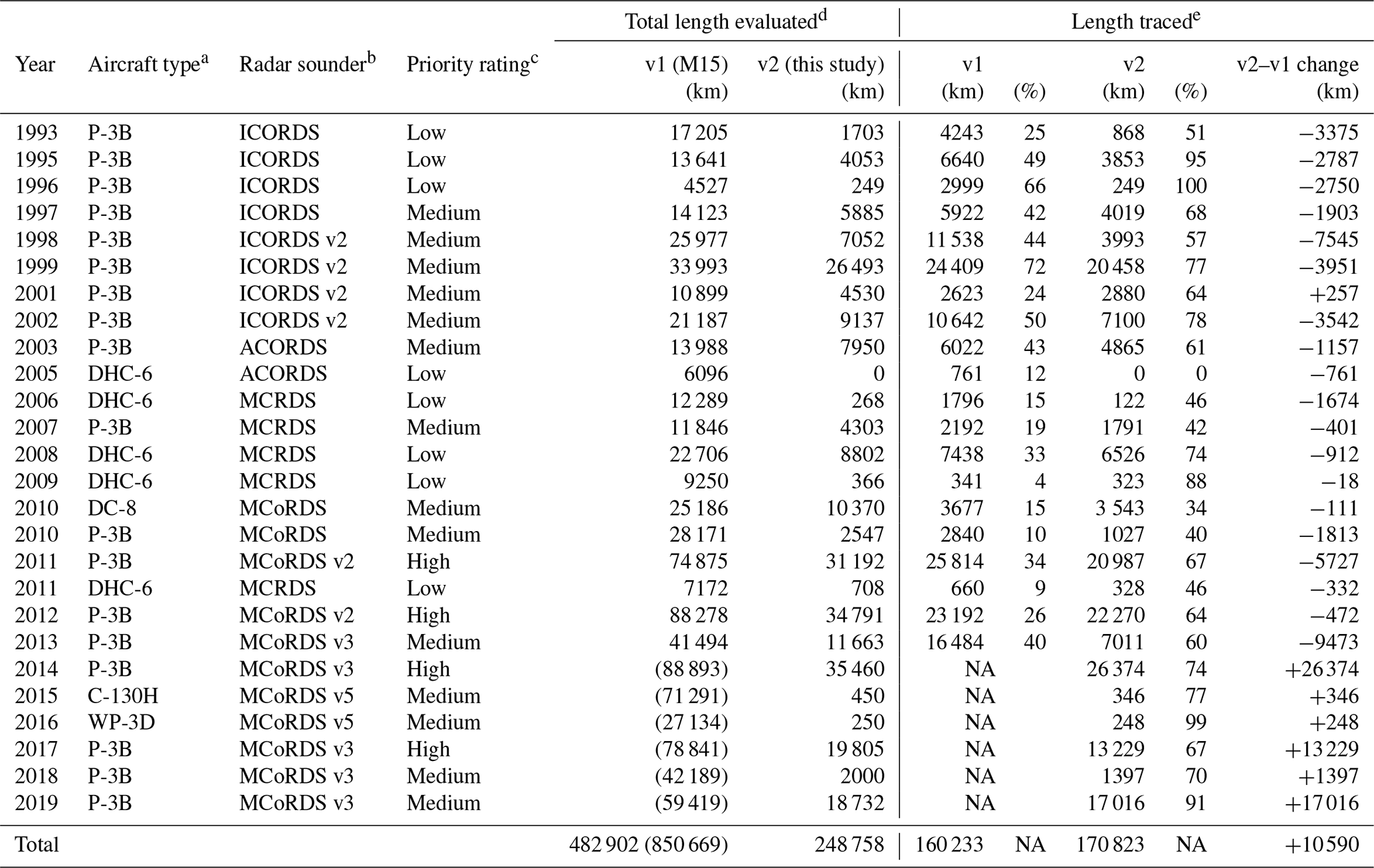
^a See MacGregor et al. (2021) for additional detail on deployed aircraft. ^b Radar sounder nomenclature follows KU/CReSIS nomenclature. They maintain a document that details system characteristics for all its surveys before 2010 (https://data.cresis.ku.edu/data/rds/rds_readme.pdf, last access: 18 June 2025). ^c The qualitative priority rating is described in Sect. 2. ^d Total length evaluated includes all segments where the radar sounder was acquiring data, which sometimes includes segments that primarily overflew Arctic sea ice that is not relevant to this study. Gaps within segments are common in earlier campaigns (1993–2001) and complicate length calculations, so here we ignore gaps greater than 10 times the median distance between traces for each segment, leading to generally lower values for those earlier campaigns than reported by M15. Values in parentheses for v1 are campaigns that were not traced by M15 because they were either not yet available (2014) or had not been flown at the time (2015–2019). For this study (v2), the total length of the reduced set for each campaign is reported. ^e Number of 1 km segments with at least one reflection traced (same metric as M15). Percentages are of the portion of the dataset evaluated, which differs between M15 and this study. NA – not available.

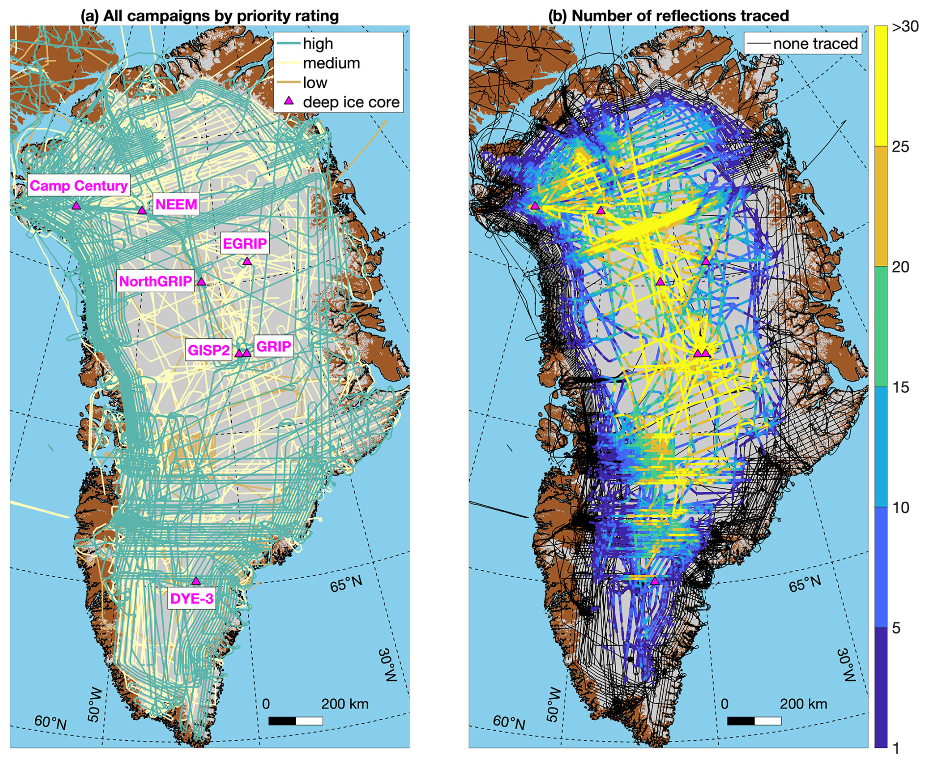
Figure 1 Airborne radar sounding surveys collected across the GrIS by KU/CReSIS between 1993 and 2019. Segments are color coded by (a) priority rating and (b) maximum number of reflections traced within 1 km along-track segments. Ice, land, and ocean masks are from Howat et al. (2014) via BedMachine v5 (Morlighem et al., 2022).

The two-way travel times of both the air–ice and ice–bed reflections have already been traced and recorded in these data by semi-automated algorithms and quality-controlled (QC'd) by KU/CReSIS personnel; the difference between these travel times has been used extensively by others to map ice thickness across Greenland (e.g., Morlighem et al., 2017, 2022). The ice–bed reflection is harder to trace confidently than the air–ice reflection, and during our examination of the dataset we occasionally observed possible errors in both. However, because we are primarily interested in reflection depths, we only adjusted the air–ice reflection travel time to address minor but obvious errors that we observed in a very small portion of the dataset that we evaluated (< 0.1 %). As for M15, when converting two-way travel time t to depth, we assume that the radio-frequency real part of the relative permittivity of ice is 3.15, equivalent to a one-way radio-wave speed in ice of 168.9 m µs⁻¹.

A fundamental difference between M15 and this study revolves around the handling of “repeat-track” flights. This difference arises from the recognition that the lead priority for most NASA airborne surveys of the GrIS by OIB and its predecessors was detecting elevation change of the surface of the GrIS using laser altimetry along the same flight tracks repeatedly (e.g., Krabill et al., 2000; Csatho et al., 2014). In other words, many NASA flights that collected high-quality VHF radar sounder data across the GrIS did so along a track that was nearly identical to another flight that did the same. M15 ignored this issue and evaluated all 1993–2013 data, which complicated subsequent reconciliation of traced reflections into an ice-sheet-wide radiostratigraphy. For example, minor variations in flight track can lead to numerous intersections of two slightly different flights, which increases the potential for incorrect matches, and having numerous closely spaced reflections can bias subsequent two-dimensional (2-D) gridding at the ice-sheet scale. In this study, we explicitly avoid tracing repeat tracks by first collating what we term the reduced set. To collate this reduced set, we first assign each campaign a priority rating (Table 1), i.e., an a priori qualitative assessment of the campaign's overall radar data quality intended to guide prioritization for further tracing. This rating was mostly based on the radar system used and known campaign outcomes, but we recognize that individual intra-campaign segment quality can vary significantly due to several factors (e.g., environmental RF noise, data-acquisition interruptions, survey altitude change, GNSS or system-timing errors). We then manually inspected a map of the GrIS showing all radar flight tracks and identified all contiguous sets of frames required to “complete” a GrIS radiostratigraphy from the 1993–2019 KU/CReSIS data. If any portion of a track was repeated, then only a portion from the campaign with the highest available priority rating was included. While this approach means that many previously traced segments from v1 of the GrIS radiostratigraphy have been effectively discarded, it minimized the work required to review those data. As a result, M15 traced at least one reflection in ∼ 33 % of the total dataset it examined, while this study more than doubled that ratio (69 %; Table 1). Table 2 summarizes this step and all other major methodological differences between M15 and this study.

Table 2 Summary of key differences between the development of the v1 (M15) and v2 (this study) GrIS radiostratigraphy datasets.

To ensure the continuity of traced reflections within individual segments and reduce the computing resources required, M15 reconfigured individual radar data frames so that they partly overlapped with each other (typically by ∼ 1 km). However, this process often created more challenges than it solved. In the intervening decade since that study, available computing resources have grown substantially but the data volume of any given SAR-processed segment from the radar systems deployed has remained the same. Here we simply concatenate contiguous sets of frames (portions of segments) as needed for the reduced set, removing any non-unique traces that are present (whether in time or space). This procedure resulted in 536 sets of concatenated radar data frames that range between 12 and 3774 km long, with a median length of 250 km. We ultimately traced at least one reflection in 496 (93 %) of those concatenated sets (Fig. 2a).

3 Reflection analysis methods

In this section, we describe the methods we used to trace GrIS radiostratigraphy, and QC and date the dataset, focusing primarily on the key differences between this study and M15, all of which were made with the intent of accelerating product development and decreasing uncertainty therein. Table 2 summarizes those key differences in our methodology for pre-processing, predicting, tracing, QC'ing, dating, and gridding GrIS radiostratigraphy. Figure 2 shows the key elements of this workflow.

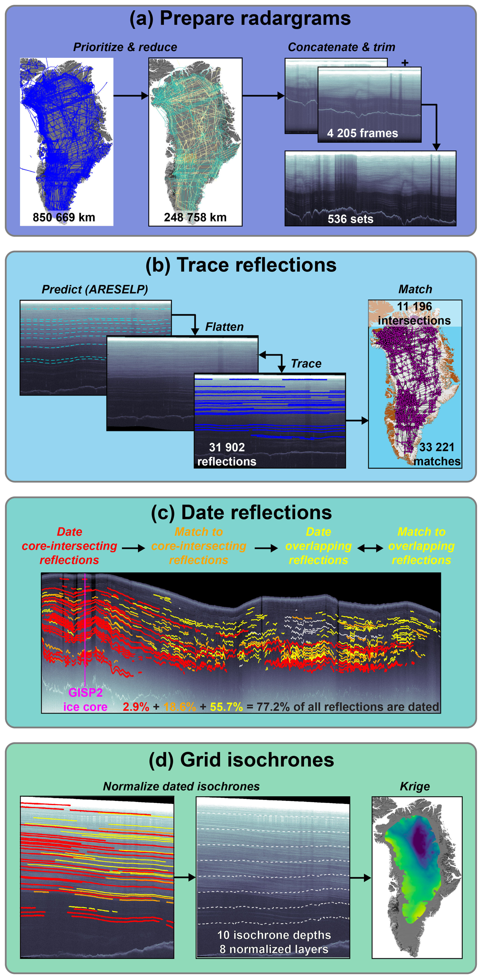
Figure 2 Flowchart illustrating the key steps involved in generating GrIS radiostratigraphy v2. Values given relate to the entire dataset, not just the radargrams shown. (a) Radargram preparation, including selection of the reduced set and concatenation (Sect. 2). (b) Typical tracing workflow and subsequent inter-segment reflection matching (Sect. 3.1, 3.2). (c) Reflection dating begins at ice cores, is sequentially propagated outward using reflections matched with core-intersecting ones, and then any remaining reflections that horizontally overlap with already dated ones are then dated where possible. The latter two steps are then repeated until no new reflections are dated. White reflections are undated (Sect. 3.3) (d). Gridding isochrones begins by vertically interpolating the dated radiostratigraphy to pre-selected ages/depths, and then each of those ages/depths are gridded two-dimensionally using ordinary kriging (Sect. 3.3).

3.1 Tracing workflow

It is much simpler to confidently trace any reflection if a prediction of its location can be generated automatically beforehand. M15 introduced two automatic methods that leveraged the phase change of the recorded complex signal to predict the slope of internal reflections and – by integrating these slopes along-track – the shape of the reflections themselves. However, these methods were limited by the availability of large-volume, single-channel complex data from KU/CReSIS, and they cannot be applied to data that have already been SAR-focused. In cases where complex data were not available (i.e., most of the 1993–2013 dataset), Automated Radio Echo Sounding Processing (ARESP) was applied, using a refactored version of the ARESP algorithm introduced by Sime et al. (2011). However, all three methods focus on estimating reflection slope, as do similar methods introduced later (e.g., Holschuh et al., 2017). As a result, it is often difficult to determine where to automatically terminate a given reflection prediction in a manner comparable to that which often occurs with observed reflections, e.g., they fade out or merge with another reflection. This challenge tends to limit the use of slope prediction methods to well-behaved radargrams with stable and relatively high signal-to-noise ratios.

Alternatively, Xiong et al. (2018) introduced an alternative method that they termed the Automated RES Englacial Layer-tracing Package (ARESELP). This method first identifies candidate reflection peaks vertically using wavelet transforms, prior to then propagating these candidate reflection peaks horizontally using Hough transforms for slope prediction. We selected this method for reflection prediction in previously untraced campaigns (2014–2019) because: (1) it does not require complex data; (2) it permits reflections to terminate; (3) it often generates realistic synthetic radiostratigraphy; and (4) the algorithm was publicly archived. We refactored the ARESELP algorithm (written in MATLAB™) to both accelerate it and improve QC of its output; we then applied it to the 2014–2019 campaigns (Figs. 2b, 3a). Despite our improvements, ARESELP is only used to predict reflection geometry and not as a substitute for tracing itself, as its output quality is variable (Jebeli et al., 2023). For example, ARESELP often identifies the multiple of the air–ice reflection as a candidate internal reflection. Where ARESELP is successful, its outputs were used only to initially “flatten” the radar data (described below) and then discarded, so that no ARESELP-predicted reflections were mistaken for operator-traced ones.

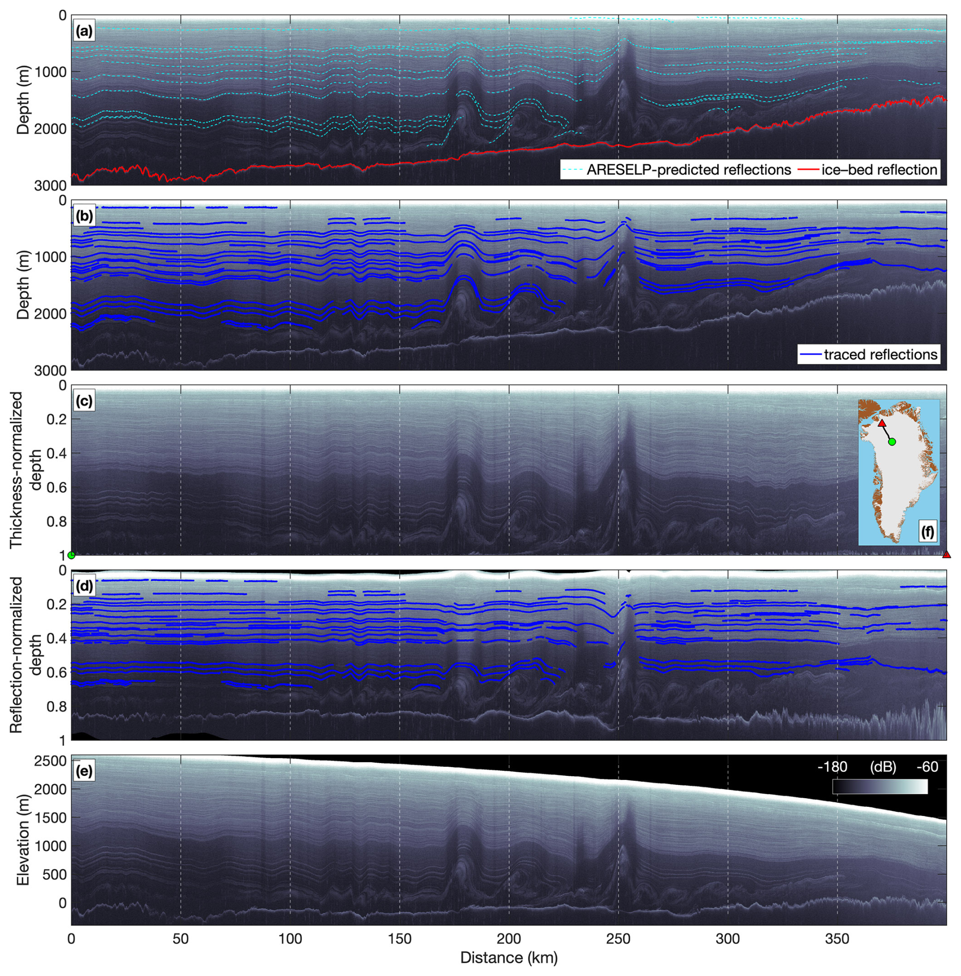
Figure 3 Multiple visualizations of a portion of a single segment (eight concatenated frames) from 13 April 2017 (20170413_01_049–056) that approximately follows ice flow from a central ice divide toward the outlet of Petermann Glacier. All radargrams shown at the same color scale. (a) Untraced radargram in terms of depth, i.e., the variable-length portion of the radargram before the air–ice reflection has been removed, with ARESELP-predicted reflections overlain. (b) Same as (a) but with traced reflections overlain. (c) Thickness-normalized radargram. (d) Reflection-flattened radargram. (e) Elevation-corrected radargram (relative to geoid). (f) Location of radargram in Greenland.

As illustrated by M15, flattening radar data with respect to predicted or already traced reflections is both a valuable QC method and one which can accelerate further tracing (Figs. 2b, 3d). Here we continue to use this method with minor adjustments that permit it to more reliably and iteratively estimate the vertical position of reflections that were not observed at the reference location, but which overlap with ones that were. However advantageous, this flattening method requires that either predicted or traced reflections are already available, which is not always the case. Inspired by earlier studies concerned with the physical interpretation of radiostratigraphy and modeling thereof, especially Nereson et al. (1998) and Hindmarsh et al. (2006), here we introduce an additional radargram reprojection that is thickness-normalized, which requires only that the air–ice and ice–bed reflections already be traced, as is the case for nearly all the KU/CReSIS dataset we evaluated. Normalization by ice thickness is commonly applied in analytic and numerical models of ice flow to ease interpretation, but to the best of our knowledge it has not previously been applied to the returned power P_r displayed in radargrams themselves, even though it can accelerate tracing. In the nomenclature of Hindmarsh et al. (2006), thickness normalization of radargrams also offers a rapid way of evaluating whether internal reflections drape over subglacial topography (i.e., they are essentially a shallower and smoother version of the ice–bed reflection) or override it (i.e., variations in reflection depth bear little resemblance to the ice–bed reflection and are mostly negligible). Following thickness normalization, draping reflections should be flatter, while overriding ones could be rougher. In practice, because relatively few of the flight tracks considered here both follow present ice flow and contain interpretable radiostratigraphy (Sime et al., 2014; Cooper et al., 2019), such a straightforward glaciological evaluation (draping vs. overriding) is often difficult. We note that alternative physically based vertical reprojections of radar data are conceivable, such as the coordinate transform for ice flow models described by Parrenin et al. (2006), but here we focus on the simplest to implement and interpret for reflection tracing.

To perform this thickness normalization, the surface and bed travel times, t_s(x) and t_b(x), respectively, are first smoothed using a 3 km-long locally weighted filter in the along-track direction x. The normalized depth coordinate $\widehat{z}$ is $\left(t-t_{\mathrm{s}}\left(x\right)\right)/\left(t_{\mathrm{b}}\left(x\right)-t_{\mathrm{s}}\left(x\right)\right)$. Because t_s(x) and t_b(x) both vary along-track, the number of fast-time samples that form the radargram between them also varies, so the vertical interval between samples $\mathrm{\Delta }\widehat{z}={\widehat{z}}_{i+\mathrm{1}}-{\widehat{z}}_i$ also varies along-track. The thickness normalization is a vertical rescaling that does not directly alter the returned power P(x,t) that constitutes the radargram, so if the vertical resolution of the displayed radargram can also vary along-track, then the thickness-normalized returned power $\widehat{P}(x,\widehat{z})$ can be displayed with no change in amplitude from P(x,t). In practice, it is simpler and more computationally efficient to display 2-D matrices with two monotonic axes. Thus, the second and final step is to vertically interpolate P(x,t) onto a single monotonic $\widehat{z}$ vector that has the same number of samples as the original radargram and ranges from zero to one, which sometimes slightly degrades the signal-to-noise ratio of $\widehat{P}(x,\widehat{z})$ relative to P(x,t). As for reflection-based flattening, reflection travel times can be similarly vertically reprojected, or traced within this projection and then reprojected to the radargram's original vertical frame of reference (t). This reprojection is simpler than that for reflection-based flattening, is also parallelizable, and is particularly valuable for initial reflection tracing within radargrams where H(x) varies substantially, as it reduces the need to adjust the vertical axis when tracing.

In terms of selecting which reflections to trace, for v2 we focused exclusively on those that we deemed most likely to be isochronal. Specifically, we focused on distinct, relatively isolated reflections in the upper ∼ 80 % of the ice column that are observed across many radargrams, are not diffuse (i.e., difficult to trace using semi-automatic peak following), and do not form part of a disrupted basal unit. While these criteria represent an effort to ensure the validity of a core assumption of our approach (reflection isochroneity), we are not aware of direct observations of unconformable reflections that are both within the GrIS interior and above disrupted basal units that contradict this assumption, as have been observed in Antarctica (e.g., Das et al., 2013). Deeper basal ice in the GrIS interior and strata exposed at the ice margin can clearly be disrupted and overturned, and are probably unconformable (Dahl-Jensen et al., 2013; MacGregor et al., 2015a, 2020; Panton and Karlsson, 2015; Bons et al., 2016; Leysinger-Vieli et al., 2018), so we mostly avoid tracing reflections within this zone unless they meet other criteria and are identifiable across a large distance or several radargrams. As a result, several deeper reflections mapped by M15, which were typically the top of disrupted basal units, were removed during our review of the v1 dataset.

We continue to use semi-automatic peak following to trace reflections, typically using a very narrow fast-time (vertical) sampling window (±1 sample; 1.7–5.3 ns, equivalent to 1.4–4.5 m, depending on campaign) between traces, but sometimes ±2 samples and rarely ±3 samples for especially steep reflections. The algorithmic speed of this method outweighs its relative simplicity, as it permits faster tracing and faster correction of the inevitable errors therein. To limit these errors, we terminate propagation of a candidate reflection automatically once another existing reflection is intersected or where tracing has propagated a prescribed distance limit from the manually selected inception (typically 25–100 km, depending on radargram quality and reflection slope) – whichever is first.

A critical addition to the tracing workflow relative to M15 is an algorithmic check for stratigraphic conformability following the tracing of any reflection or modification thereof. This QC check simply requires that the sign (either > 0 or < 0) of the depth difference between any pair of reflections be both non-zero and the same throughout the radargram. In other words, no traced reflection can be both above and below another. This check automatically identified occasional tracing errors in the v1 radiostratigraphy that we rectified, and it simplified the process of QC'ing v2. Once tracing is complete, all reflections were vertically readjusted by $\le \pm \mathrm{1}$ fast-time (vertical) samples to match the local maximum in P_r. This adjustment also increases the value of recorded reflection P_r values for future investigations (e.g., MacGregor et al., 2015b).

3.2 Inter-segment matching

Once tracing was complete, intersections between traced segments were identified automatically, with an algorithm that requires a minimum intersection angle of 5° between segments in map view and limits identified intersections to a maximum along-track density of 5 km within any given segment. The combination of the reduced set and these intersection selection criteria generated 24 % fewer intersections than v1 (11 196 vs. 15 148), which simplifies subsequent reflection matching (Fig. 2b). Assuming a uniform reflection matching error rate, fewer matching errors will be made if there are fewer intersections to evaluate.

Matching reflections between traced segments and between distinct radar systems is a significant challenge for large radiostratigraphic datasets. While M15 evaluated automatic matching, they ultimately did not use it. Here we generate an initial set of reflection matches automatically, with an algorithm that limits inter-segment matches to those with a mean depth difference no more than three times the maximum range resolution of the segment pair's radar system (2.4–4.4 m for most systems considered) within 500 m of their intersection. These automatic matches were then QC'd using network graphs to verify stratigraphic conformability between reflection pairs, using an algorithm like that applied when tracing individual segments (Sect. 3.1), i.e., if a segment contains two reflections that overlap horizontally, then they cannot both be matched to the same reflection in another segment. Additional matches were then identified manually, which were then again QC'd using network graphs. In M15, matches were not permitted between the earliest campaigns (1993–1997) and later ones due to their difference in range resolution; here we permit such matches since prominent traced reflections were often similar across all campaigns.

3.3 Dating and gridding

Once traced, matched, and merged, reflections must be dated to be of maximum value to the broader scientific community. Our dating algorithm is mostly unchanged from M15, to which we refer the reader for further details. We are unaware of any substantive improvement in reflection dating methodology developed since then, although alternatives exist if better estimates of accumulation histories or modern dielectric profiling ice-core data are available (Cavitte et al., 2021; Franke et al., 2025). To date traced radar reflections across an ice sheet, multiple dated and synchronized ice cores are required. We use the same six deep ice-core depth–age scales as M15 (their Table 2) but supplement them here with the addition of the partially complete EastGRIP (EGRIP) depth–age scale from Mojtabavi et al. (2020). This depth–age scale includes the upper 1884 m of the ice column – approximately three quarters thereof given an ice thickness of ∼ 2550 m – which records the period 0–15 ka. Compared to M15, we slightly relax the search radius within which a radar segment is considered to have “intersected” an ice core from 3 to 5 km, increasing the number of core intersections from 53 to 65. The use of the reduced set (no repeat tracks) also decreases dependence on the Camp Century ice core, which was overrepresented in the v1 dataset (47 % of all intersections, as compared to 31 % in this study). We continue to use the “quasi-Nye” dating method introduced by M15 to vertically interpolate the age of undated reflections that are either sandwiched between or are vertically near pairs of dated reflections (no more than the thickness of a dated layer pair or 20 % of the ice thickness, whichever is less). This method seeks the best-fit vertical strain rate that can match the depth–age relationship of the two bounding reflections and then uses this vertical strain to interpolate the age of the undated reflection – or extrapolate where appropriate (Fig. 2c).

Previously, an undated reflection could only be dated if it did not cause the vertical profile of age anywhere in the segment to decrease with depth. Here we relax this requirement slightly to accommodate potential matches of vertically closely spaced reflections by instead requiring that the age of the putative dated reflection be within 5 % of the uncertainty in age of adjacent dated reflections. This relaxation accommodates slight mismatches in age between reflections that intersect different ice cores. Finally, where sufficient dated reflections exist, we use quasi-Nye interpolation to estimate the along-track depth of a set of “synthetic” isochrones at predetermined ages. We include the same set of five ages generated by M15 (9, 11.7, 29, 57, and 115 ka) along with five more of additional paleoclimatic interest from the Late and Early Holocene, the bounds of the Bølling–Allerød period during the Last Glacial Period, and an approximate Last Glacial Maximum (3, 8, 12.8, 14.7, and 19 ka; Rasmussen et al., 2006).

Like M15, we use ordinary kriging to grid the depths of the 1-D along-track isochrones onto a 2-D grid using the Python geostatistical simulation software package GStatSim (v1.0.6; MacKie et al., 2023). We also use quasi-Nye interpolation (M15) to infer the age at predetermined thickness-normalized depth intervals along all traced segments and then grid these ages as well. We select a 5 km grid in the standard EPSG:3413 projection – rather than 1 km as in M15 – to focus on the large-scale age structure of the ice sheet. Contrary to M15, we find that absolute depths are smoother at large scale than thickness-normalized depths, so we grid the former instead. We find that a zero-nugget spherical semivariogram model is a better representation of the experimental semivariogram of shallower/younger isochrones (≤ 19 ka), while an exponential model is better suited to deeper/older ones. For the age at regular depth intervals, we restrict the gridding to the middle 70 % of the ice column (10 %–80 % ice thickness) at 10 % intervals as this depth range captures the range of most traced reflections (Figs. 2d, 4); we find that spherical variograms are most suitable at all depths. This normalized depth range is more conservative than for M15 (4 %–100 % ice thickness at 4 % intervals). Independent variogram models are applied to each depth/age, as opposed to a single variogram model as in M15. We apply a 2-D Gaussian smoothing filter to all the resulting grids to reduce noise from individual traced segments and fill in small, enclosed gaps using natural neighbor interpolation. Finally, we blank out any portions of the grid that would result in age overturning (unconformities) relative to other adjacent grids.

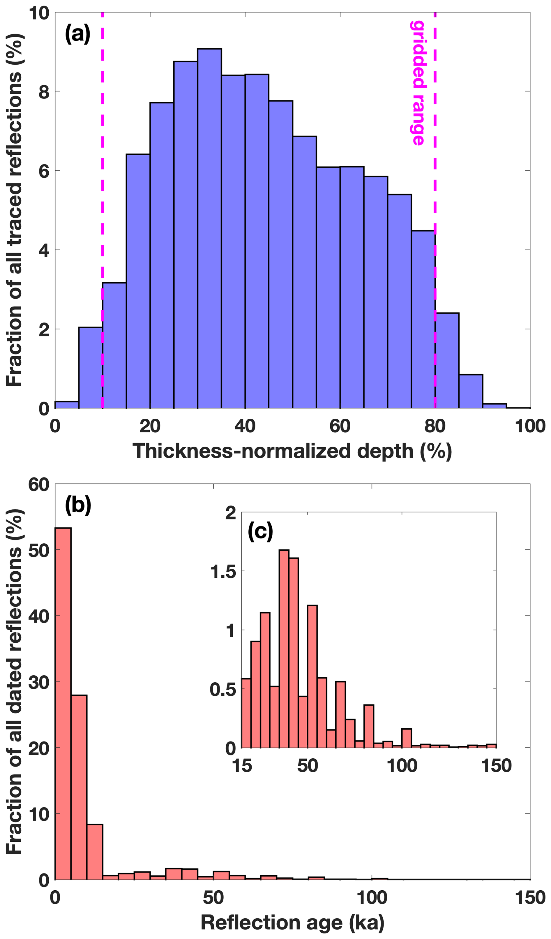
Figure 4 (a) Histogram of the normalized depth of all traced reflections (both dated and undated). Vertical magenta dashed lines highlight the normalized depth range for which the age of the ice sheet is gridded. (b) Histogram of the age of dated reflections. (c) Zoom-in of panel (b) on the pre-Holocene age range.

3.4 Depth and age uncertainty estimation

The depth uncertainty of the traced reflections is principally attributable to the assumed radio-wave velocity in pure ice and a correction for spatiotemporally variable firn air content. As for M15, we assume that the real part of the radio-frequency complex relative permittivity of pure ice ${{\mathit{ϵ}}^{\prime }}_{\mathrm{ice}}$ is 3.15, equivalent to a radio-wave velocity in ice v_ice of 168.9 m µs⁻¹. M15 did not directly apply a firn correction and instead attributed a constant and uniform 10 m depth uncertainty to all traced reflections. Since then, substantial progress has been made in the modeling and validation of the firn air content in the near-surface of ice sheets, due to its importance for interpretation of satellite altimetry data (e.g., Medley et al., 2022). The total firn air content is equivalent to the firn correction that is commonly applied to radar sounding data to correct reflection depths. Here we use the modeled firn air content developed by Medley et al. (2022) for the period 1980–2021 across Greenland and Antarctica to determine the local firn correction for each radar trace from the nearest 5 d simulation interval to the acquisition date. We then assume that the reflection depth uncertainty associated with the firn correction is reduced to 5 m. The median modeled firn correction applied is ∼ 19 m, but it can be up to ∼ 25 m.

The age uncertainty for each dated reflection is calculated following the same methods described in further detail by M15. For core-dated reflections, this total age uncertainty is the combination of the reported uncertainties in the ice-core depth–age scales (unchanged from M15), the depth uncertainty of the reflection (discussed above), and the uncertainty induced by the range resolution of the radar system used. The latter quantity depends on the signal-to-noise ratio (SNR) of the reflection at its closest approach to the ice core, which is typically ∼ 5 dB, so for simplicity we assume that quantity is uniform for all core-dated reflections. For reflections dated using quasi-Nye dating, an additional uncertainty is included that accounts for the interpolation/extrapolation of age, which is based on the age uncertainties of the existing dated reflection pair and the variance of the interpolated/extrapolated age across the overlapping section (Eq. 12 in M15).

To estimate the uncertainty of the 2-D grids, we first also vertically interpolate the along-track depth (age) uncertainty of dated reflections to the age (depth) of interest and then krige these quantities using the same variogram model parameters as for their respective age (depth) of interest. These kriging-derived uncertainties are then combined with the kriged uncertainty for the parameter of interest (depth or age) as the square root of the sum of squares (M15 only considered the latter term).

4 Results

The generation of the reduced set, where we downselect repeat flight tracks to a single instance acquired with the highest-fidelity radar system, substantially reduces the number of radargrams that must be examined to generate a complete GrIS radiostratigraphy from NASA/NSF airborne radar sounding data. For this second version of the radiostratigraphy dataset (v2), we reviewed only 36 % of the 1993–2013 radargrams, as compared to 100 % for v1. However, we recorded a traced reflection in 65 % of the 1993–2013 radargrams examined (112 213 of 172 062 km), as compared to 33 % for v1 (160 233 of 482 903 km). While we preserved fewer line kilometers of reflections for 1993–2013, we added 58 610 km from 2014–2019 acquired using generally higher-fidelity radar systems.

GrIS radiostratigraphy v2 contains 31 902 individual traced reflections of widely varying lengths. Of these reflections, 2.9 % were dated “directly” where they intersected ice cores, 18.6 % by automatically or manually identified matches to those core-dated reflections, and another 55.7 % using quasi-Nye dating, leaving 22.8 % of traced reflections undated (Fig. 2c). Direct core-dating of reflections is essential but – following our tracing strategy – results in a very limited spatial distribution of dated reflections, mostly following the northern part of the central ice divide (Fig. 5). Reflections matched to those core-dated reflections significantly expand the coverage of dated reflections, especially in central and northern Greenland. Farther south, where reflections become discontinuous, age interpolation of dated reflections is especially important between ∼ 65 and 71° N. Undated reflections remain mostly around the periphery of the GrIS, in fast-flowing regions such as Sermeq Kujalleq, and in southern Greenland south of ∼ 68° N.

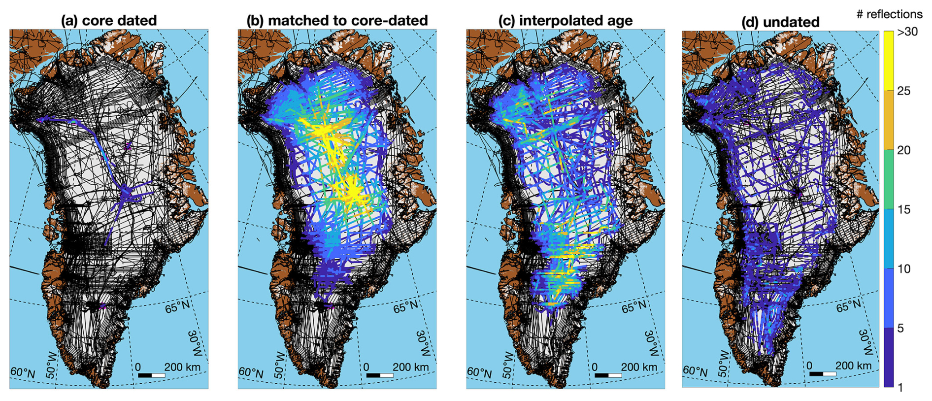
Figure 5 Number of traced reflections by the method in which they were dated.

For completeness and validation we generated Movie S1, which shows all traced segments in an elevation-corrected reference frame. This movie illustrates both the breadth of the traced reflections and the considerable number of untraced reflections, which are typically discontinuous and less distinct – but not exclusively so. Most (94 %) reflections were traced in a depth range within 10 %–80 % of the ice thickness, following both our stated prioritization, signal loss with increasing depth, and the challenge of tracing distinct very shallow reflections within most of the KU/CReSIS dataset that we evaluated. The large majority (86 %) of all dated reflections are from the Holocene (11.7–0 ka; Fig. 3b), which is consistent with previously observed patterns of radar reflectivity across the ice sheet. Some of the most distinct reflections are from the Last Glacial Period (115–11.7 ka), in particular the well-known trio observed throughout northern Greenland (37.7, 44.7, and 50.7 ka, respectively), so they are also often some of the most contiguous or readily matched between segments so they tend to be underrepresented in the distribution of all dated reflections compared to numerous and sometimes difficult-to-match shallower Holocene reflections.

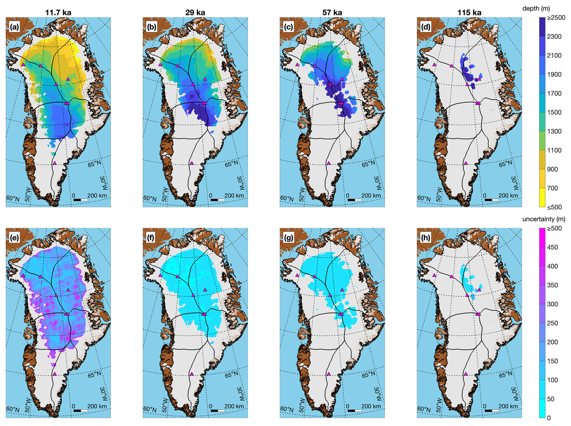
Figure 6 (a–d) Gridded depth of four out of the 10 gridded synthetic isochrones (11.7, 29, 57, and 115 ka, respectively). (e–h) Gridded uncertainty in these isochrones. Ice drainage basins (black lines) are from Mouginot et al. (2019).

The resulting depth/age grids cover up to 65 % of the ice sheet by area (Figs. 6 and 7). The uncertainties in the resulting datasets also are slightly more completely expressed than by M15. In comparison to similar depth/age grids produced by M15, it is clear that producing a dated GrIS radiostratigraphy within ∼ 100 km of the ice margin or south of ∼ 68° N remains challenging. Neither version of the dataset does so consistently, except for v1 along parts of the northern margin of the GrIS, which we attribute to less conservative kriging parameters than those applied in this study. We attribute this broader challenge not to the sparsity of surveys (Fig. 1) but rather to the absence of traceable radiostratigraphy (less common) or the low continuity of observed radiostratigraphy (more common), which makes it less feasible to trace efficiently using this study's methods and was not prioritized (Movie S1). This result is consistent with earlier automated assessments of radiostratigraphic continuity by Sime et al. (2014) and M15, particularly in terms of where traceable radiostratigraphy is present (although not necessarily dateable).

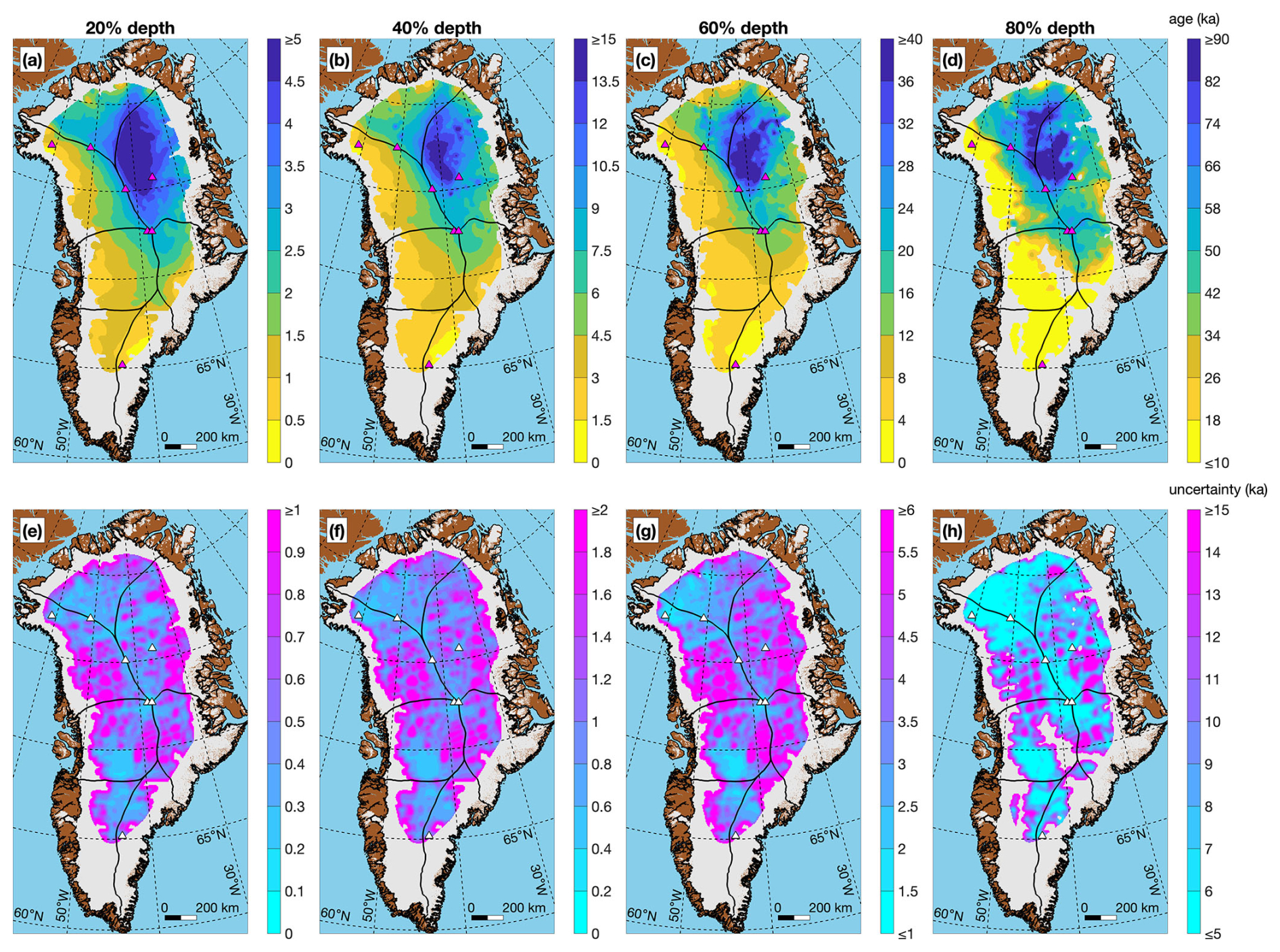
Figure 7 (a–d) Gridded age of four out of the seven gridded ages at 20 %, 40 %, 60 %, and 80 % of ice thickness, respectively. (e–h) Gridded uncertainty in these ages. Note each panel has a different color scale, whereas for each row of Fig. 6 the color scale is the same.

As observed by M15 and reproduced here, the oldest ice at most depths is observed in the southeastern portion of the northernmost ice drainage basin and the northwestern portion of the northeastern drainage basin (northwest of the Northeast Greenland Ice Stream). Any potentially conformable Eemian ice (130–115 ka) is likely also located there (Fig. 6d). These results are qualitatively consistent with observations of outcropping pre-Holocene along the northern margin of the GrIS (MacGregor et al., 2020). Any substantial (> 100 m) conformable layer of pre-Holocene basal ice is likely absent south of ∼ 65° N, which is consistent with the higher long-term accumulation rates there (e.g., MacGregor et al., 2016a).

The gridded uncertainty of the synthetic isochrones (Fig. 6e–h) varies significantly and does not necessarily increase with depth. Assuming comparable relative uncertainties for all dated reflections, it also depends on proximity (in age) of the synthetic isochrone to dated reflections. While reflections were regularly traced near the onsets and terminations of the Bølling–Allerød period (14.7–12.8 ka), the Younger Dryas cold period (12.8–11.7 ka), and the Holocene epoch (11.7 ka–present), much more common are yet younger reflections (Fig. 4a) from which the depth of those onsets/terminations was sometimes estimated. In contrast, the prominent trio of older reflections previously mentioned that are often observed together in the northern GrIS represent a more spatially limited but stronger constraint on the location of some older climate transitions (e.g., Fig. 4f, g).

This study's gridded fields are generally similar to those in M15 (Fig. 8). We attribute most differences to improved coverage and QC in this study, the more conservative coarser grid resolution (5 km vs. 1 km), and the final smoothing applied. For the isochrone depths, as expected the differences increase toward the ice margin and away from ice core sites with a slight trend toward increasing magnitude with increasing isochrone age. The gridded age differences display a more complex spatial pattern. Their differences are lower at shallower depths, as expected, but increase significantly at 60 % depth, particularly in the older northern and northeastern drainage basins. At 80 % depth – the maximum normalized depth we considered – the magnitude of the differences is large but varies in sign, with an increasing magnitude trend toward the north.

Franke et al. (2023) presented multiple gridded isochronal datasets for the northern GrIS from OIB and other campaigns led by the Alfred Wegener Institute (AWI), which could be compared to our gridded products. However, because they gridded directly traced isochrones, rather than the synthetic isochrones at climate transitions that we focused on, based on the ages of their isochrones alone most of our gridded isochrones are not directly comparable with theirs. Only one is potentially comparable with our 11.7 ka isochrone (Fig. 8a), which is their 12.0 ka isochrone for the Petermann Glacier onset region. However, given the two-order-of-magnitude difference in grid resolution between their isochrone (0.05 km) and ours (5 km), along with the smoothing we applied, we do not consider such a comparison meaningful.

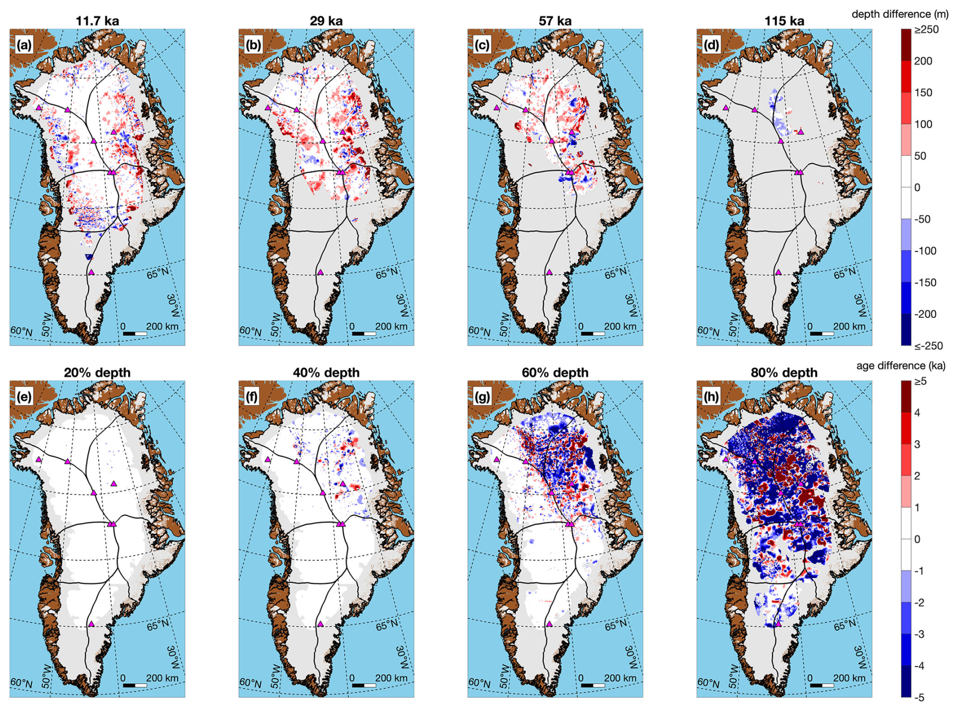
Figure 8 (a–d) Difference in gridded depth of four isochrones mapped by this study from M15. (e–h) Same as above, except for the age at normalized depths.

5 Discussion

Much has been written about the potential value of – and the challenge of producing – large-scale ice-sheet radiostratigraphy datasets (e.g., Karlsson et al., 2013; Sime et al., 2014; Moqadam and Eisen, 2024; Bingham et al., 2024). As with all methods of observation or data analysis, future improvements therein are almost inevitable. However, at some point the unique capabilities of the system in question – whether they be resolution, speed, accuracy, or some other characteristic – must be locked so that the observation or analysis of interest can be made. Both M15 and this study assessed several methods for accelerating tracing but – critically – eventually paused that assessment and shifted gears to the actual production of an ice-sheet radiostratigraphy. This production stage revealed several challenges associated with QC'ing, dating, and normalizing a large-scale radiostratigraphy (e.g., Fig. 2; Sect. 3), but several subsequent related studies have focused mostly on designing or assessing alternative methods for tracing or slope estimation (e.g., Panton, 2014; Delf et al., 2020), with relatively few that consider dating reflections not observed at ice cores (Cavitte et al., 2021). Further, it is now well established that it is relatively easy to trace many reflections in any one of the two dozen or so high-quality KU/CReSIS VHF radargrams that cross the northern GrIS (Fig. 1b; e.g., Panton, 2014; Xiong et al., 2018). It is much harder to trace discontinuous reflections within ∼ 300 km of the ice margin, harder still within ∼ 100 km, and even harder to confidently propagate ages from interior ice cores toward the periphery.

Despite the clear advantage of scale provided by our approach to mapping radiostratigraphy, our current approach possesses some limitations that could be addressed in future versions. A primary limitation is that while the GrIS radiostratigraphy v2 dataset depends critically on the spatial relationships between segments and the matches between their traced reflections, it is not a modern relational database through which updates to any individual element propagate automatically. Instead, it is a series of static datasets developed in sequence (concatenated radargram segments, traced reflections, inter-segment reflection matches, reflection ages, and gridded depths/ages). In other words, if an error in tracing any reflection is identified and adjusted, then any matches between that reflection and others must be manually reverified and the dating and gridding procedures would need to be rerun. A second but more tractable challenge is the dynamic display of intersecting segments and associated traced reflections on 2-D radargrams, which would clarify how far to attempt to trace reflections to maximize the potential for matching them between segments. Alternatively, such inter-segment relationships can sometimes be obvious in three-dimensional (3-D) perspectives of intersecting radargrams and their traced reflections (e.g., Franke et al., 2023). However, we experimented extensively with such 3-D perspectives in both MATLAB™ and PyVista (Sullivan and Kaszynski, 2019) and found that modifying or matching mapped radiostratigraphy remains cumbersome in three dimensions when evaluating many segment intersections (11 196 in this study).

To address the challenge of extracting useful geophysical information from large data volumes, machine learning (ML) methods have been increasingly deployed in many fields of Earth science. The constellation of ML methods clearly possesses great potential for accelerating the tracing of radiostratigraphy, but they face several broad challenges before they can be widely adopted (Moqadam and Eisen, 2024; Moqadam et al., 2025; Peng et al., 2024). First, most ML methods use supervised learning, which typically requires large training datasets. In this case, such datasets would be radargrams that have been traced exhaustively, i.e., those that possess few or no false negatives. However, all presently available large-scale radiostratigraphy datasets – including the one presented in this study – left innumerable observed reflections untraced. These reflections were typically less distinct, less bright, or shorter, and so were deprioritized in our workflow (Sect. 3.1). We suggest that suitable ML methods for tracing radiostratigraphy are those that can better tolerate inevitable and copious false negatives, perhaps by being trained on synthetic radargrams or using ARESELP-generated predictions (Culberg and Schroeder, 2021; Jebeli et al., 2023). A second and related issue is the question of which reflections should be traced. An answer with a future ML application in mind could simply be “all of them,” but perhaps a more realistic and readily achievable answer is “those that models seek to match.” In the latter more restrained scenario, which was implicit in our tracing strategy, we may consider both which observed reflections are clearly distinct from others and those which models seek to reproduce to better resolve ice-sheet history, i.e., typically those associated with or close to major climate transitions (e.g., Born and Robinson, 2021; Sutter et al., 2021). However, how to enable ML to perform a similar prioritization remains unclear. Third, as emphasized by Delf et al. (2020) and applicable to all automated methods for tracing radiostratigraphy, improving our ability to automate the matching of reflections across discontinuities – whether due to an acquisition malfunction or observation limitation such as steep reflection slopes – remains an outstanding challenge, and it is not yet clear how ML can accelerate this process.

As originally conceived, this dataset (GrIS radiostratigraphy v2) would have included additional VHF airborne radar sounding data collected primarily by institutions besides the US (Fig. 9). These include the first such data collected across the GrIS during the 1970s by a Danish–British–American consortium that was recently digitized by Karlsson et al. (2024), surveys of the northern and central GrIS mostly from the 1990s led by AWI (e.g., Nixdorf and Göktas, 2001), and more recent AWI surveys using newer CReSIS-built radar systems (e.g., Kjær et al., 2018; Franke et al., 2022, 2023; Jansen et al., 2024). Including these data was ultimately beyond the scope of this study but remains possible and could help fill remaining gaps in coverage, especially in the northern half of the GrIS. A potential challenge in incorporating these data would be their different center frequencies and bandwidths, which result in different patterns of interfering reflections – particularly in reflection-rich Holocene ice. For the newer AWI data (2016–present), this challenge is due to the higher center frequency and wider bandwidth of the system used that would typically result in more reflections being distinguishable, whereas for the other, mostly older, data the challenge is reversed. Because we found that certain distinct reflections could be matched between KU/CReSIS systems from 1993 all the way through to 2019, there is reason for cautious optimism in merging such disparate datasets. Further, there is precedent in Antarctica for similar multi-system reconciliation of radiostratigraphy (Bodart et al., 2021; Winter et al., 2017; Cavitte et al., 2021; Franke et al., 2025), and the bandwidth of some of the older AWI data (short chirp mode) or the newer AWI data operated in narrowband mode is comparable to most of the radar systems considered here. For the older 1970s data, their greater geolocation uncertainty may also present an additional challenge in matching reflections with those from newer systems.

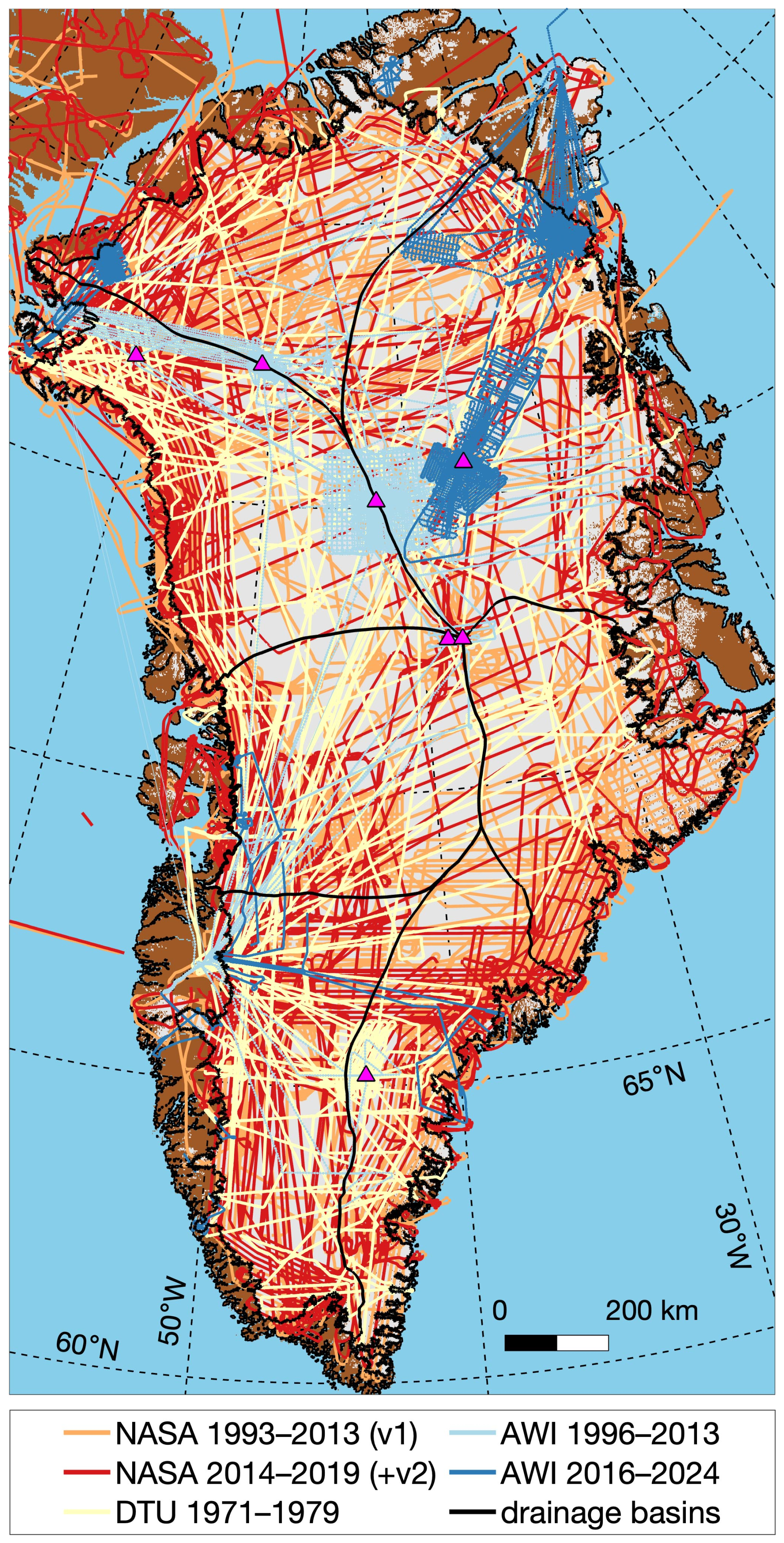
Figure 9 Airborne radar sounding surveys collected across the GrIS led by various institutions that could be included in future versions of a GrIS radiostratigraphy (AWI: Franke et al., 2023; Olaf Eisen and Daniel Steinhage, personal communication, 2020; DTU: Karlsson et al., 2024), as compared to that collected primarily by NASA/KU/CReSIS between 1993 and 2019.

Table 3 Format of the “segment” structure in the MATLAB™ file for each campaign that contains the traced reflections at the radargram resolution.

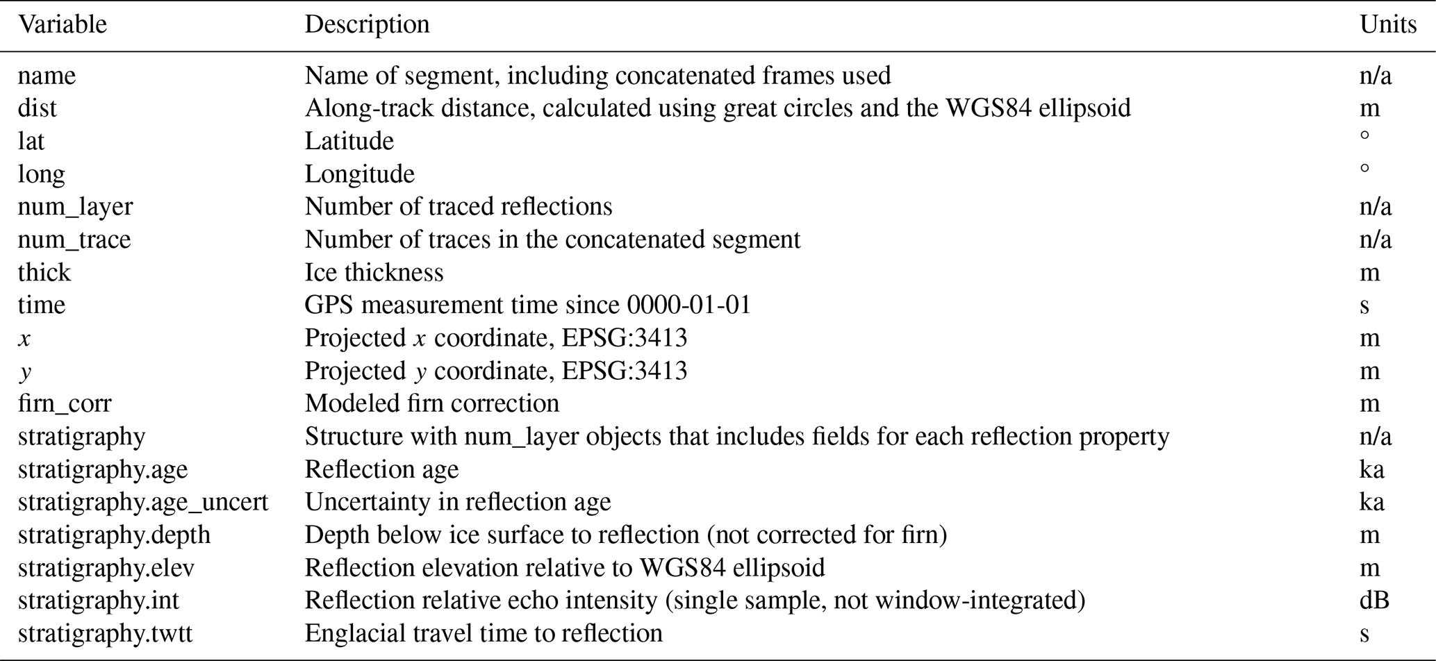
n/a – not applicable.

Table 4 Format of GeoPackage files for each concatenated segment that contains the traced reflections at the radargram resolution.

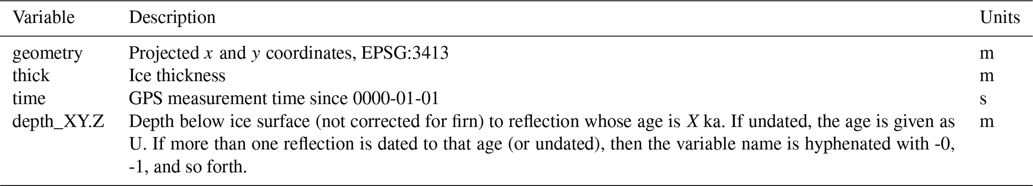
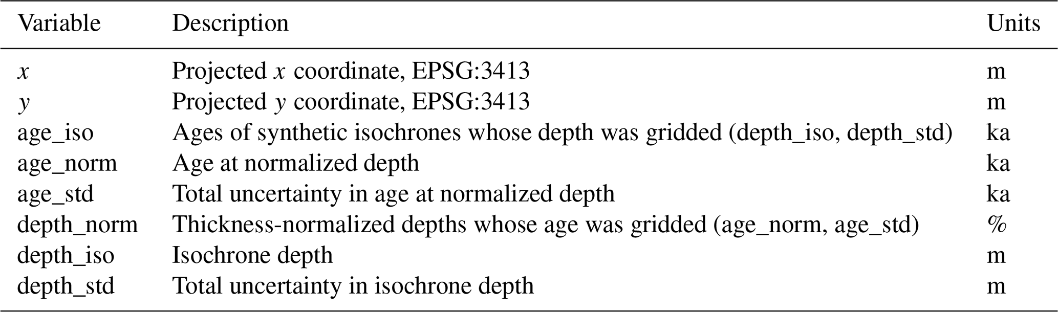
Table 5 Format of NetCDF file that contains the gridded isochrone depths and ages at normalized depths.

Given its improved spatial coverage, more robust QC, and more accessible data formatting (Sect. 6), we expect that this second version of the GrIS-wide radiostratigraphy will help fully realize part of the original purpose for generation of the M15 dataset – to “[provide] a new constraint on the dynamics and history of the [GrIS]” – but also to expand the range of potential applications for such a dataset. The v2 gridded products can be used to evaluate the modern age structure of initialized ice-sheet models to validate their overall climate sensitivity and various model parameterizations, especially past accumulation rates (e.g., Born and Robinson, 2021; Sutter et al., 2021; Rieckh et al., 2024). Following the methods introduced by those recent studies, the capability to record and advect ice age non-diffusively using a Lagrangian approximation was also introduced recently (in v2.1) to the widely used Parallel Ice Sheet Model (https://www.pism.io/, last access: 18 June 2025; e.g., Aschwanden et al., 2019), which expands the potential user base for model evaluation of the age structure of the GrIS. At coarser scales, the gridded datasets can be more reliably used to distinguish between Holocene and pre-Holocene ice, which is valuable for radiometric studies of radargrams (e.g., MacGregor et al., 2015b; Chu et al., 2018) and interpretation of bulk rheology (e.g., MacGregor et al., 2016a). Finally, the along-track traced reflections can be used to rapidly identify anomalous structures within the ice sheet that can be either diagnosed simply using steady-state models (e.g., MacGregor et al., 2016b) or targeted for more detailed diagnosis using structural analyses (e.g., Franke et al., 2022).

6 Code and data availability

The MATLAB™ GUIs, functions, and scripts and Jupyter notebooks used to perform the analysis and generate the figures in this paper are available at https://doi.org/10.5281/zenodo.14183061 (MacGregor, 2024a). Most of the analysis was performed using functions built in to several versions of MATLAB™ (R2022a to R2024b) with its associated Image Processing, Mapping, Statistics, and Wavelet toolboxes. Python v3.12, various standard packages, and GStatSim were used to krige the dataset (MacKie et al., 2023).

The datasets resulting from this study, which together constitute version 2 of Greenland's deep radiostratigraphy, are available at https://doi.org/10.5281/zenodo.14182641 (MacGregor et al., 2025) and may also be later made available through the National Snow and Ice Data Center, where further dataset-specific documentation will be provided. Table 3 describes the format of the HDF-5-compatible MATLAB™ (v7.3 .mat) files that contain each campaign's traced reflections for each segment. Table 4 describes the format of the GeoPackage (.gpkg) files that contain the depths of each segment's traced reflections, as we anticipate that these will be the most widely used reflection properties. These GeoPackage files are a more openly accessible version of the MATLAB files, but include many fewer reflection properties due to limitations of the format. Reflection ages and age uncertainties are preserved in each GeoPackage file's metadata. Table 5 describes the format of the NetCDF (.nc) file that contains the gridded (5 km horizontal resolution) isochrone depths and ages at normalized depths (Sects. 3.3, 4). For brevity, in these three tables we describe only the key variables and not all preserved metadata or other attributes.

7 Conclusions

We produced a second version of a dated radiostratigraphic dataset covering a substantial portion (up to 65 %) of the GrIS using a non-repeating subset of available NASA/NSF radargrams. While far from comprehensive, as innumerable minor reflections were left untraced – let alone dated – this dataset represents an improved and potentially large-scale constraint on models of the flow of the GrIS and their sensitivity to past climate change. The inferred basic age structure of the GrIS is not significantly changed from that which M15 first described, but its development was simplified, and the resulting dataset has substantially fewer tracing errors, is more self-consistent, and is expected to be more robust for future modeling efforts. This version of the dataset continues to indicate that the oldest ice in Greenland is likely in the northern central GrIS, that the ice sheet is significantly older in northeastern and far northern Greenland, and that the radiostratigraphy and age structure of the GrIS south of 65° N remains challenging to map using presently available data and techniques. Finally, we modernized and further generalized the tools used to generate this radiostratigraphy – as compared to the previous version of the dataset – and expect that they could be used to either improve upon this dataset in the future for the GrIS or to accelerate Antarctic-wide mapping of radiostratigraphy.