Quantitative imaging datasets of surface micro- to mesoplankton communities and microplastic across the Pacific and North Atlantic oceans from the Tara Pacific expedition

This paper presents the quantitative imaging datasets collected during the Tara Pacific expedition (2016–2018) carried out on the schooner Tara. The datasets cover a wide range of plankton sizes, from microphytoplankton (> 20 µm in size) to mesozooplankton (a few centimetres in size), and non-living particles such as plastic and detrital particles. It consists of surface samples collected across the North Atlantic and the North and South Pacific Ocean from open-ocean stations (a total of 357 samples) and from stations located in coastal waters, lagoons or reefs of 32 Pacific islands (a total of 228 samples). As this expedition involved long distances and long sailing times, we designed two sampling systems to collect plankton while sailing at speeds of up to 9 knots. To sample microplankton, surface water was pumped aboard using a customised pumping system and filtered through a 20 µm mesh size plankton net (hereafter referred to as the deck net – DN). A high-speed net (HSN; 330 µm mesh size) was developed to sample the mesoplankton. In addition, a manta net (330 µm) was also used, when possible, to collect mesoplankton and plastics simultaneously. We could not deploy these nets at the reef and lagoon stations of islands. Instead, two bongo nets (20 µm) attached to an underwater scooter were used to sample microplankton. In addition to describing and presenting the datasets, the complementary aim of this paper is to investigate and quantify the potential sampling biases associated with these two high-speed sampling systems and the different net types, in order to improve further ecological interpretations. Regarding the imaging techniques, microplankton (20–200 µm) from the DN and bongo net were imaged directly aboard Tara using a FlowCam instrument (Fluid Imaging Technologies), whereas mesoplankton (>200 µm) from the HSN and manta net were analysed in the laboratory with a ZooScan system (back on land). Organisms and other particles were taxonomically and morphologically classified using the automatic sorting tools of the EcoTaxa web application; following this, validation or correction was carried out by taxonomic experts. For microplankton smaller than 45 µm, a subsample of 30 % of the annotations was 100 % visually validated by experts. More than 300 different taxonomic and morphological groups were identified. The datasets include the metadata and the raw data from which morphological traits such as size (equivalent spherical diameter) and biovolume were calculated for each particle as well as a number of quantitative descriptors of the surface plankton communities. These descriptors include abundance, biovolumes, the Shannon diversity index and normalised biovolume size spectrum, allowing the study of their structures (e.g. taxonomic, functional, size and trophic structures) according to a wide range of environmental parameters at the basin scale (https://doi.org/10.5281/zenodo.6445609, Lombard et al., 2023).

1 Introduction

Zooplankton serve as an important conduit for the transfer of energy from primary producers to higher trophic levels (Ikeda, 1985). In this key position in the food webs, they also play an important ecological and biogeochemical role (Turner, 2015; Steinberg and Landry, 2017), with associated ecosystem services. In particular, they are essential to Pacific fisheries management, as they influence fish productivity and ecosystem dynamics (Balachandran and Peter, 1987; Guo et al., 2019; Hays et al., 2005). The datasets that we present here cover a wide diversity of surface plankton, ranging from 20 µm to few centimetres in size, at the scale of the Pacific Ocean. The vastness and unique characteristics of the Pacific Ocean make it a particularly interesting study area. From nutrient-rich upwelling or island zones to oligotrophic gyres, the diverse oceanic processes of the Pacific Ocean present a wide range of environmental conditions that significantly influence plankton communities, making it a key region for plankton research (Chavez et al., 2011; Longhurst, 2007). However, zooplankton sampling efforts in the Pacific Ocean have largely focused on the temperate North Pacific, eastern and western boundary currents in the North Pacific, leaving vast areas undersampled (Drago et al., 2022). This gap is particularly evident in the NOAA zooplankton dataset (https://www.st.nmfs.noaa.gov/copepod/atlas, last access: 3 June 2025), where the undersampling is particularly true for the central subtropical and tropical Pacific, in which fisheries are important resources for the thousands of Pacific islands. We present a map (Fig. 1) overlaying updated zooplankton databases with samples from the Tara Pacific expedition, illustrating how these new data address sampling gaps. Global mapping of zooplankton in the Pacific is hindered by the highly expansive operational ship time required to cover this vast ocean. The use of high-speed sampling, such as the Continuous Plankton Recorder (CPR) survey (by Hardy in 1926), the Longhurst–Hardy Plankton Recorder (LHPR) survey (Longhurst et al., 1966), the Gulf III OCEAN Sampler (Gehringer, 1958) and the Gulf V plankton sampler (Sameoto et al., 2000), and newer low-tech designs (cruising-speed net, CSN, in Von Ammon et al., 2020; Coryphaena in Mériguet et al., 2022), including the one employed in our datasets, provides valuable opportunities to expand sampling coverage and frequency and, thus, address this undersampling. In the hope of increasing zooplankton sampling efforts with a similar cruising speed, we discuss the benefits, challenges and limitations of this high-speed sampling approach based on the lessons learnt from obtaining these datasets.

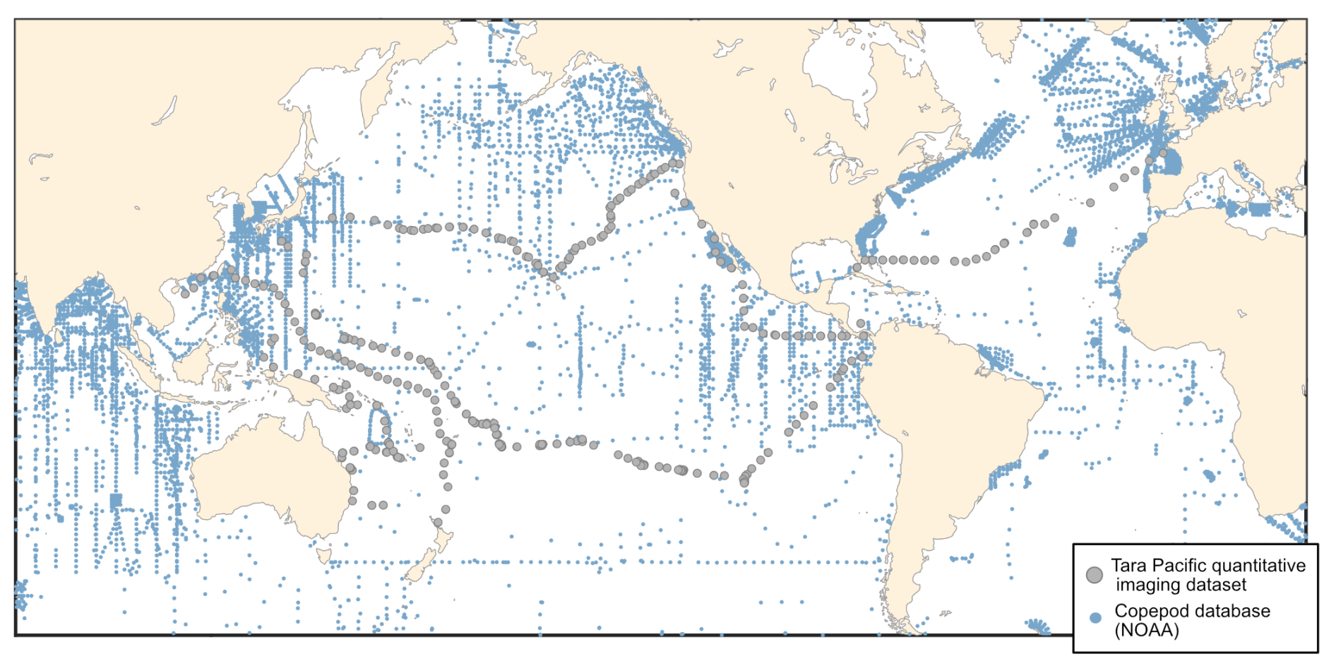
Figure 1 The spatial distribution of zooplankton observations from the COPEPOD database (https://www.st.nmfs.noaa.gov/copepod/, last access: 3 June 2025; all groups) is represented by blue points. Plankton imaging data (>20 µm) from the Tara Pacific expedition are shown in grey.

Therefore, the aim of this paper is to present and discuss these open-access quantitative plankton imaging datasets sampled during the Tara Pacific expedition (2016–2018), conducted in the Pacific Ocean. In general, the effects of different environmental forcings on plankton are often focused on one size range of plankton or on a particular taxonomic or functional type to the exclusion of others. It is often difficult to reconcile different methods of analysis (e.g. taxonomic, biogeochemical or genomic) to provide a coherent view of plankton as a whole. In this respect, quantitative imaging is complementary to other methods to study plankton community composition (e.g. high-performance liquid chromatography, HPLC; flow cytometry; or genomics), as it simultaneously provides quantitative measures of abundance, morphology and biovolume (as a proxy for biomass) for different taxonomic groups of plankton organisms (Lombard et al., 2019). The datasets represent a diversity of surface plankton analysed with the use of two quantitative imaging instruments: (1) a FlowCam (Sieracki et al., 1998), which images microplankton from 20 to 200 µm, and (2) a ZooScan (Gorsky et al., 2010), which images mesozooplankton (>200 µm). The dataset also includes the plastics imaged by the ZooScan. Overall, it encompass a total of 2 356 231 images, including both surface micro- and mesoplankton and non-living particles, such as plastics, making a significant contribution to improving the availability of plankton data.

These datasets are of great value because of the relative rarity of sampling efforts directed at surface planktonic communities at the oceanic scale. Potential limitations of the data presented here are discussed below. To ensure adequate spatial coverage while also considering navigation constraints, we designed two new sampling systems to collect surface micro- and mesoplankton while sailing at a maximum speed of 9 knots. The “Dolphin” sampler was designed to pump seawater into a 20 µm net on board, the “deck net” (DN), whereas the “high-speed net” (HSN) was designed and towed to collect surface plankton larger than 300 µm in size (see Gorsky et al., 2019, for details). In addition to these high-speed sampling devices, although with less extensive spatiotemporal coverage, a manta net (330 µm) was also used whenever the cruising speed allowed for it (i.e. <4 knots), and it collected surface mesoplankton and plastics. Two bongo nets (20 µm), towed by an underwater scooter, were also used by scuba divers around islands, reefs and lagoons. Thus, a complementary objective of this paper was to study and quantify the potential sampling biases of the different methods used during this expedition, in order to maximise the quality of the data offered to the scientific community and promote similar high-speed zooplankton sampling efforts which strongly enhance the spatial coverage of samples. Another characteristic of these datasets is the daytime sampling of surface (0–1 m) plankton communities. This offers the possibility of geographic intercomparisons and interdisciplinary studies related to the ocean's surface layer, enabling direct comparisons with other surface measurements, such as satellite and atmospheric data. However, this raises questions about the quantitative nature of the sampling itself, particularly regarding the representativeness of the datasets. While these datasets provide quantitative accuracy by offering all of the necessary information to consistently calculate estimates of the sample content, we must warn that the data may not fully be “quantitatively representative” of the broader ecosystem. Although the sampling objective is to sample the surface layer, daytime sampling alone cannot document the nocturnal intrusion of migrating zooplankton and micronekton to the surface. It is worth mentioning that night sampling was also operated for zooplankton alone (see Fig. 10 in Gorsky et al., 2019); however, these data do not spatiotemporally reconcile with day sampling and were, therefore, not analysed in priority.

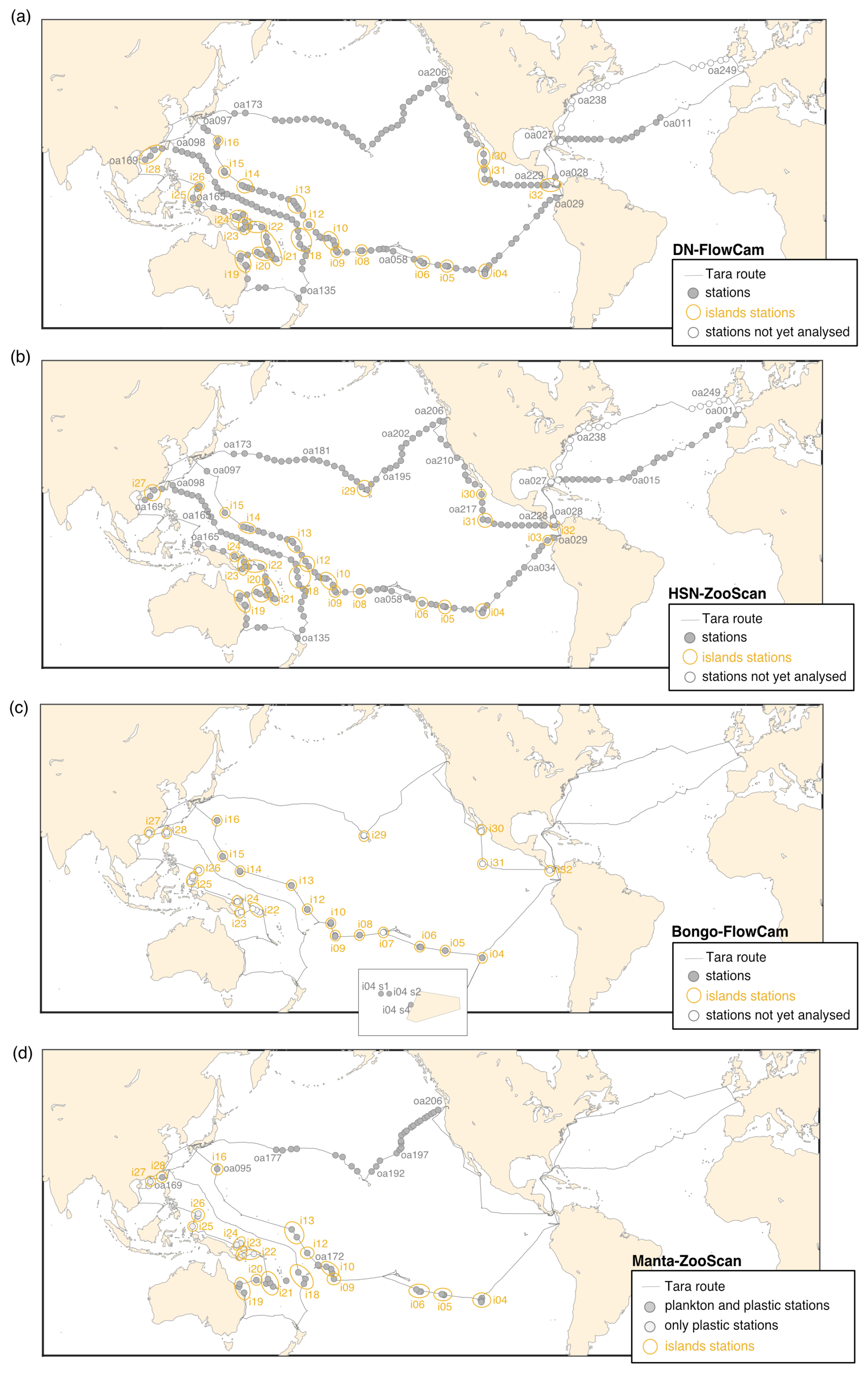
Figure 2 Tara Pacific expedition (2016–2018) sampling map for the four different datasets. The respective top two panels show continuous sampling with (a) DN–FlowCam and (b) HSN–ZooScan, whereas the respective bottom two panels present more discrete sampling, with a focus around islands, with (c) bongo–FlowCam and (d) manta–ZooScan (plankton and plastic samples). Island stations, stations within 200 nmi of an island, are represented inside yellow circles. The not-yet-analysed stations in the figure legend refer to samples that have not yet been scanned for the ZooScan dataset and have not been taxonomically validated for the FlowCam dataset.

2 Methods

2.1 Sampling

We present a collection of FlowCam and ZooScan images acquired during the Tara Pacific expedition (2016–2018; Gorsky et al., 2019; Lombard et al., 2023). All samples and protocol names in this article follow Lombard et al. (2023) in order to help the user match the samples and associated data presented here with other samples from the expedition. Sampling was generally carried out at a daily frequency with sampling every ∼150–200 nmi (nautical miles) during daytime, resulting in a total of 249 sampling events labelled [oa001] to [oa249] (Fig. 2). The first 28 sampling events occurred during the trans-Atlantic crossing as the ship sailed from France to the Pacific. At the end of the expedition, the schooner Tara acquired quantitative imaging samples at stations [oa232] to [oa249] across the North Atlantic. Data have been published on the SEANOE platform to allow for future updates and the completion of datasets. The plankton sampling covers a wide latitudinal range (temperate, subtropical and tropical) and a diversity of environments associated with different oceanic regimes (equatorial upwelling, coastal upwelling, eastern boundary current, subtropical gyres and other provinces). We collected over 357 samples in the open ocean and 228 samples close to reefs or in lagoons. A selection of 32 coral reef island systems (labelled [i01] to [i32]) in the tropical and subtropical Pacific Ocean were targeted for coral reef holobiont studies (Planes et al., 2019), including surface plankton sampling analysed by quantitative imaging. A summary of geological, topological and human population characteristics of the different islands targeted (e.g. name, size, elevation and human population) can be found in Lombard et al. (2023). Any sampling event that was conducted within an exclusive economic zone (EEZ) of an island (defined as the area that stretches 200 nmi or 370 km out from the coastline of the island in question) was considered to be an island station and annotated with the island label [i##_oa###]. All other sampling events were considered open-ocean stations (high seas, 132 open-ocean stations) and were annotated using [i00_oa###].

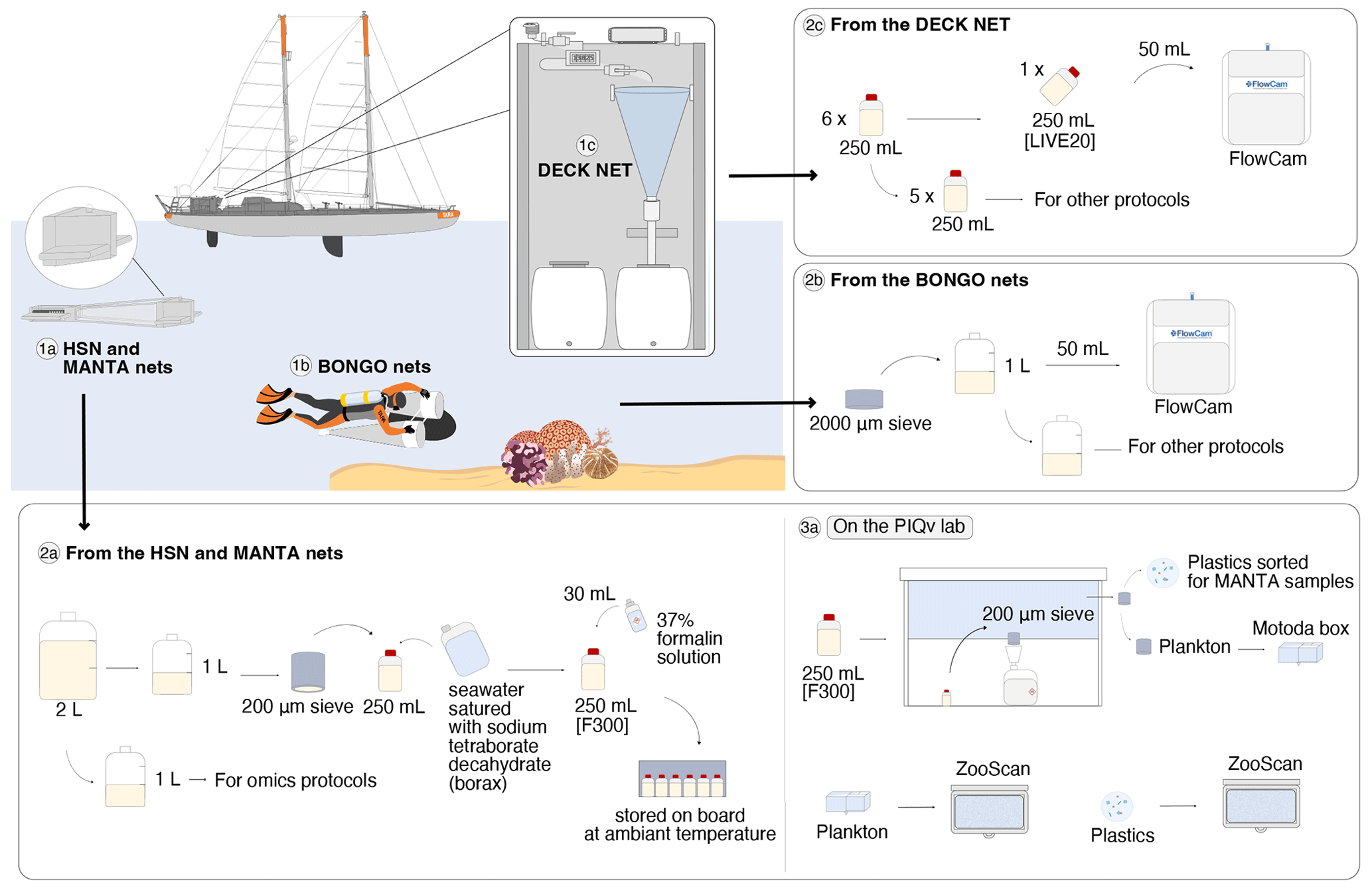
Figure 3 Schematic overview of the sampling events and protocols used during the Tara Pacific expedition for quantitative imaging. The top-left panel corresponds to the sampling events with the deployed plankton nets: (1a) the 330 µm high-speed net (HSN) and the 333 µm manta net, (1b) the 20 µm bongo nets attached to the underwater scooter, and (1c) the 20 µm deck net (DN) on the deck of the Tara. Samples from the DN (2c) and bongo nets (2b) were imaged live with the FlowCam (20–200 µm), whereas samples from the HSN and manta net (2a) were imaged with the ZooScan (>300 µm). For the ZooScan analysis, samples were fixed using formaldehyde, stored on board and analysed on the Imaging Quantitative Platform (PIQv) in the laboratory in Villefranche-sur-Mer; the protocols for this platform are detailed in panel (3a) “On the PIQv lab”. Some drawings were taken from Lombard et al. (2023) and modified (credit Noan Le Bescot).

2.1.1 Deck net sampling

Surface water samples were collected using a custom-built water-pumping system named Dolphin. It consists of a stainless-steel pyramidal frame with a front aperture (0.04 m wide and 0.40 m high) and is deployed from the starboard side of the ship (see pictures in Gorsky et al., 2019). The Dolphin was used underway (while sailing) and was connected to a peristaltic pump (max flow rate of 3 m³ h⁻¹) mounted on the deck of the schooner Tara. The system is equipped with a flowmeter to record flow rates. The pumped water was filtered through a 20 µm net (deck net) that was mounted on the wall of the wet lab (see panel 1c in Fig.  3 as well as pictures in Gorsky et al., 2019). Before entering the deck net, the pumped water passed through a 2000 µm mesh filter. Deck net pumping lasted 1 to 2 h, depending on the plankton concentration. Samples were divided into subsamples: one subsample was employed for quantitative microplankton imaging analysis on live samples (LIVE20; panel 2c in Fig. 3), whereas the remaining material was used for specific protocols detailed in Lombard et al. (2023). Further information on the Dolphin system, the deck net and various protocols based on this sampling can be found in Gorsky et al. (2019) and Lombard et al. (2023).

2.1.2 Bongo net sampling

Plankton larger than 20 µm were sampled at ∼2 m below the sea surface using two small-diameter bongo plankton nets with a 20 µm mesh size and an opening area of 0.071 m². These nets were towed by divers using underwater scooters (panel 1b in Fig. 3) for about 15 min at maximum speed (0.69±0.04 m s⁻¹). Each net was equipped with a flowmeter rated to provide accurate measurements at speeds above 0.3 m s⁻¹, but the relatively low maximum speed of the underwater scooter was insufficient to allow seawater to flow through the 20 µm mesh fast enough to trigger the rotation of the flowmeter. Therefore, the volume was estimated from the tow speed and tow duration using the following expression:

$$\begin{array}{}\text{(1)}& \mathrm{bongo}\mathrm{volume}=\mathrm{0.071}\times \mathrm{tow}\mathrm{speed}\times \mathrm{tow}\mathrm{duration}.\end{array}$$

2.1.3 HSN and manta net sampling

Concomitantly with the deployment of the Dolphin to collect microplankton, the high-speed net (HSN) was towed to sample mesoplankton. The HSN was equipped with a 330 µm mesh and designed to be deployed while sailing at up to 9 knots (average speed of deployment was 6.7 knots). The HSN features the same mouth opening as the Dolphin system, consisting of a stainless-steel pyramidal frame with a front aperture measuring 0.40 m × 0.04 m (see the zoomed-in view of the HSN mouth system in Fig. 3). The base opening of this pyramidal structure measures 0.34 m × 0.34 m. This net was deployed from the starboard side and towed at a distance of 50–60 m behind the ship (to avoid it being in the wake of the ship) for a period of 60–90 min (depending on the plankton density). In addition to the HSN, a manta net was also deployed in some locations (Fig. 2). Manta nets have a rectangular frame with a 0.16 m × 0.60 m mouth opening and a 4 m long net with a 333 µm mesh size, and they were used at a maximum speed of 3 knots for an average of 30–40 min.

Flowmeters were mounted at half of the opening height above the bottom of the opening on both HSN and manta nets to ensure that they (the flowmeters) were well submerged during deployment while measuring the filtered volume. Theoretical volumes were calculated by accounting for a three-quarter mouth opening of the HSN and manta nets, 0.3 m × 0.04 m and 0.6 m × 0.12 m, respectively (see Eqs. 3–5). As these nets are surface nets, the water collected actually passed through three-quarters of the opening height (see photos of deployments in Gorsky et al., 2019). To calculate volumes from the flowmeter for the HSN, we considered an opening of 0.34 m × 0.34 m, corresponding to the dimensions of the pyramid base opening where the flowmeter was positioned inside the HSN (Eq. 2). We compared the volume estimated from the flowmeter readings with theoretical estimation using the towing distances. We computed the towing distances using the minute-binned latitude and longitude recorded with the Tara's GPS along each deployment. We calculated the distance between the start–end latitude and start–end longitude for each minute in order to calculate the distance per minute covered by the boat. We then summed these “per-minute” distances over the duration of the deployment to obtain a calculated distance that is as close as possible to the true towing distance and accounts for potential modification of the boat's heading during deployments. The equations for calculating the filtered volumes are outlined in the following. The 0.3 factor in the flowmeter volume equation corresponds to the impeller pitch, as recommended by HYDRO-BIOS, to convert the number of revolutions into towing distance.

$$\begin{array}{}\text{(2)}& {\displaystyle }\begin{array}{rl}\mathrm{HSN}\mathrm{flowmeter}\mathrm{volume}& =\mathrm{flowmeter}\mathrm{end}\\ & -\mathrm{flowmeter}\mathrm{start}\times \mathrm{0.3}\\ & \times \left(\mathrm{HSN}\mathrm{mouth}\mathrm{opening}\mathrm{area}\right)\end{array}\text{(3)}& {\displaystyle }\begin{array}{rl}\mathrm{HSN}\mathrm{theoretical}\mathrm{volume}& =\mathrm{tow}\mathrm{distance}\\ & \times \left(\mathrm{HSN}\mathrm{mouth}\mathrm{opening}\mathrm{area}\right)\end{array}\text{(4)}& {\displaystyle }\begin{array}{rl}\mathrm{Manta}\mathrm{flowmeter}\mathrm{volume}& =\mathrm{flowmeter}\mathrm{end}\\ & -\mathrm{flowmeter}\mathrm{start}\times \mathrm{0.3}\\ & \times \left(\mathrm{manta}\mathrm{mouth}\mathrm{opening}\mathrm{area}\right)\end{array}\text{(5)}& {\displaystyle }\begin{array}{rl}\mathrm{Manta}\mathrm{theoretical}\mathrm{volume}& =\mathrm{tow}\mathrm{distance}\\ & \times \left(\mathrm{manta}\mathrm{mouth}\mathrm{opening}\mathrm{area}\right)\end{array}\end{array}$$

Simplified metadata in .csv format provide both flowmeter and theoretical volumes for the HSN and manta net, enabling the user to select the filtered volume for the calculation of quantitative descriptors. A discussion of the biases associated with each estimate is given in Sect. 3.2. The filtered volumes uploaded as metadata in EcoTaxa (EcoTaxa export table in .tsv; see Sect. 2.5) and used to compute quantitative descriptors (see Sect. 2.5) are the theoretical volumes calculated from the distance (see the results of technical validation Sect. 3.2.1).

Once recovered, samples collected both by the HSN and the manta net followed the same procedure (see panel 2a in Fig. 3). The sample was divided into two 1 L fractions (details in Gorsky et al., 2019). One fraction was concentrated on a 200 µm sieve and resuspended in a 250 mL double-sealed bottle using filtered seawater saturated with sodium tetraborate decahydrate (borax), fixed with 30 mL of 37 % formalin solution, and stored at room temperature for taxonomic and morphological analysis by imaging methods in the laboratory (samples named [F300]). The other fraction was used for omic analysis.

2.2 Acquisition and treatment of plankton imaging data

Sample labels were annotated by different users at different times during the expedition and are, therefore, not homogeneous. In order to avoid confusion or misunderstanding with respect to the labelling of the samples, an additional column has been created in the .csv simplified metadata (the “Homogenous sample names” column) with homogeneous names for all datasets.

2.2.1 FlowCam analysis

Samples from the DN (250 mL) and bongo net (50 mL) were imaged live directly on board using a FlowCam Benchtop B2 series (Fluid Imaging Technologies; Sieracki et al., 1998) equipped with a ×4 objective and a 300 µm deep glass flow cell to examine the microplankton samples (size range 20–200 µm; panel 2c in Fig. 3). Each sample was first passed through a 200 µm sieve to remove large objects that could clog the FlowCam imaging cell. Samples were then diluted or concentrated to achieve the optimum object flow. The auto-image mode was used to image the particles in the focal plane at a constant flow rate.

2.2.2 ZooScan analysis

The ZooScan imaging instrument (Gorsky et al., 2010) was used to study the mesoplankton. Samples collected from the HSN and manta nets ([F300]) were imaged at the Quantitative Imaging Platform (PIQv) of the Institut de la Mer de Villefranche (panel 3a in Fig. 3). In addition, preserved zooplankton samples have been stored in the Collection Center for Plankton of Villefranche (CCPv). The formaldehyde solution was replaced by filtered seawater during the analysis.

HSN and manta net plankton sample analysis on the ZooScan

Before scanning on the ZooScan, plankton samples were divided using a Motoda splitter (Motoda, 1959) to obtain a concentration of approximately 1000–2500 objects per subsample. This sampling strategy correctly accounted for the many small organisms as well as the large ones that might be undersampled when subsampling with the Motoda box. This limit ([1000–2500] objects) was defined by the PIQv platform to avoid the overlap of planktonic organisms, while also retaining enough organisms to give a reliable quantitative measurement of the sample. After each scan, a quality control was systematically carried out concerning (i) the quality of the scanned image and (ii) the number of objects imaged, to ensure that the number of objects was within the limits given above. The quality control tool for imaging data is accessible on the PIQv website: https://sites.google.com/view/piqv/ (last access: 3 June 2025). After treatment in the ZooScan, all samples were re-concentrated on a 200 µm sieve and resuspended in a 250 mL double-sealed bottle using filtered seawater saturated with borax, fixed with 30 mL of 37 % formalin solution, and returned to the CCPv.

The borax (sodium tetraborate decahydrate) used as a buffer may form crystals grains (that form white crystals). If the borax solution was not filtered sufficiently, crystals would end up in the plankton samples, be digitised and be counted as objects. Thus, if borax was not filtered sufficiently, white crystals may represent a large proportion of the objects within the 1000–2500 limit and, therefore, bias the quantitative measurement of the plankton. We identified 24 samples containing borax crystals during the analysis. Thus, prior to scanning, these samples were thoroughly rinsed with filtered seawater through a 300 µm mesh sieve to remove a maximum number of borax crystals from the sample. A 200 µm mesh sieve was placed below the 300 µm sieve in order to conserve the initial sample in the collection (CCPv). Analysis on the ZooScan was performed from the 300 µm sieve.

Plastic sampling from manta nets

Samples from the manta nets were gently transferred to a Petri dish. Plastic-like particles were manually separated from other components such as wood, zooplankton and organic tissues (panel 3a in Fig. 3). Entangled pieces of plastic were picked up manually from zooplankton and aggregated under a stereoscopic dissecting microscope, using forceps. The visual criteria used to classify a microfibre as synthetic were the absence of cellular structures and scales on the surface, a curved shape with a uniform surface, a uniform thickness along the entire length of the filament, spots, and strong strands (Barrows et al., 2018; Hidalgo-Ruz et al., 2012). Each sample was examined twice to ensure the detection of most of the plastic particles. Isolated plastic particles were then imaged via ZooScan. To minimise the plastic contamination of the samples, a quality control approach was undertaken following the protocol described by Pedrotti et al. (2022).

2.3 Image processing

For FlowCam and ZooScan, the full methodology used can be found in their respective manuals (https://sites.google.com/view/piqv/piqvmanuals/instruments-manuals, last access: 3 June 2025; for the ZooScan instrument, the protocol by Jalabert, 2021, is also available on Zenodo). Images generated by FlowCam and ZooScan were processed using the ZooProcess software, which extracts segmented objects as vignettes, in ImageJ (Gorsky et al., 2010). During this process, each vignette was associated with a set of 46 morphometric measurements for object characterisation, including grey levels, fractal dimension, shape and size, which were imported into the EcoTaxa web application (Picheral et al., 2017) for taxonomic classification. For ZooScan, the ZooProcess software includes a tool that enables the digital separation of potentially touching or overlapping objects in the original image. If two objects (possibly two plankton organisms) are touching, they are considered to be a single vignette and assigned a single label, which could therefore bias estimates of abundance and size, as described in Vandromme et al. (2012). Objects that were still touching after the application of the ZooProcess automatic tool were identified and separated using the ZooProcess manual separation tool to improve the quality of the subsequent taxonomic annotation, counts and size structure analysis of the zooplankton. For each ZooScan dataset, this quality control step was systematically performed during taxonomic annotation.

2.4 Taxonomic identification

Using image recognition algorithms on EcoTaxa, predicted taxonomic categories were validated or corrected by trained taxonomists. For the majority, the taxonomic classification effort was possible up to the genus level, whereas rare cases could be classified up to the species level. A number of organisms could not be reliably taxonomically identified due to a lack of identification criteria and were, therefore, grouped into temporary categories (t00x) following similar morphological criteria. Nine different trained taxonomists from the PIQv platform annotated FlowCam and ZooScan vignettes on these datasets. Annotations of FlowCam and ZooScan vignettes from the different nets were also done by different taxonomists, but the list and the global criteria to identify a group were common. To reduce operator bias between taxonomists and to ensure taxonomic consistency, a final stage of homogenisation was carried out by two taxonomists after all vignettes had been validated. At the time of the publication of these datasets, copepod genera had not been homogenised for ZooScan, but homogenisation will be pursued in the future and the published SEANOE dataset will be updated accordingly. Overall, these datasets have been published on the SEANOE flexible platform, which allows updates and corrections, so that taxonomic annotations can be improved over time. All vignettes with taxonomic annotations are visible on the open-access project in EcoTaxa (Sect. 4).

2.5 Case of FlowCam taxonomic identification for objects smaller than 45 µm

The Tara Pacific settings for the FlowCam live analysis generates many more images than the ZooScan. For example, for station oa140, the ZooScan counts 1435 images compared to 42 915 images for the FlowCam. Given that taxonomists annotated images on an image-by-image basis, the validation or correction of the automatic classification of these numerous FlowCam images would require a much higher time investment than for the ZooScan samples. In addition, the resolution of the FlowCam images of the smallest organisms does not allow us to classify them properly or at a sufficient precision. Therefore, we validated only 30 % of the total images smaller than 500 pixels (equivalent to an equivalent spherical diameter of ∼45 µm), randomly picked, assuming that this random 30 % subsample leaves a statistical count that is sufficiently representative of the population. Prior to this choice, a series of tests were conducted to assess the impact of different fractions of image validation at varying object size thresholds. Samples were randomly selected, and 100 % of the images were taxonomically validated. Subsequently, a series of simulations (three times for the four samples, with random sampling each time) were conducted to assess the impact of varying size thresholds (i.e. from 200 to 600 pixels, equivalent to 18 to 55 µm, with a step of 50 pixels) on the proportion of total images to be annotated (fractions from 5 % to 50 %, with increments of 5 %). We compared the results of these simulations using the relative root-mean-square error (RMSE). The RMSE values were divided by the total number of 100 % validated values and multiplied by 100 to express the cumulative error as a percentage. Results are shown in Fig. 4 and illustrate the cumulative error across the absolute abundance values. For our chosen threshold of 500 pixels and subsets at 30 % (highlighted in bold in Fig. 4), we observed induced errors of 0.02 %. In Fig. 4d, we present the absolute abundance and taxonomic group composition of plankton from the four samples that were 100 % taxonomically annotated, alongside the same four samples that were only 30 % (<500 pixels) annotated. These samples show highly comparable results with respect to both absolute abundance and taxonomic composition (data not shown). We carried out the same analysis as described in Fig. 4 for the total size spectrum (slope of the normalised biomass size spectrum) and for the taxonomic composition (relative abundance). They showed an induced error of 20 % and 12 %, respectively. This supplementary analysis can be found in Appendix C. The ZooProcess 8.27 software, available on the PIQv website, now includes the capability for subsampling on FlowCam data.

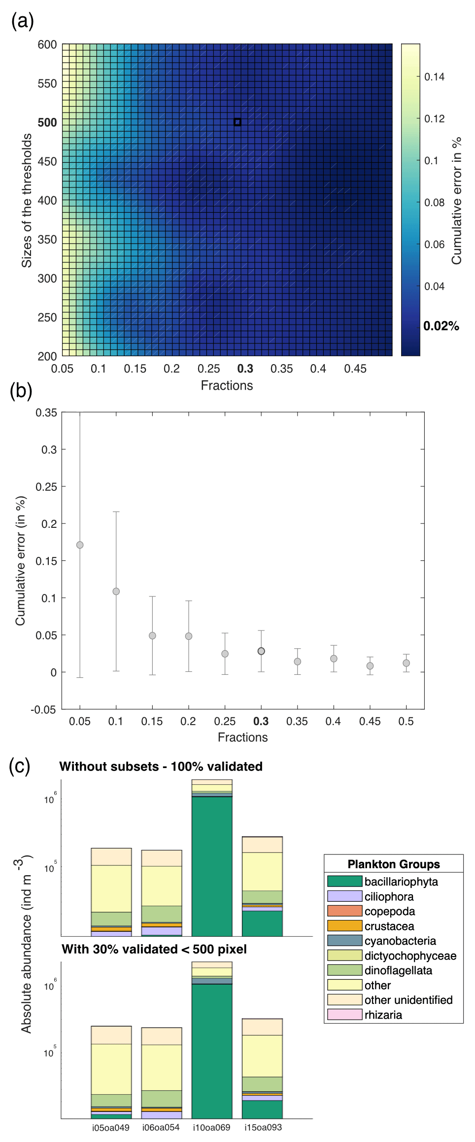
Figure 4 (a) Estimated cumulative error associated with the partial validation of particles below a size cut-off threshold ranging from 200 to 600 pixels and validated fractions ranging from 5 % to 50 %. Errors are computed as the percentage root-mean-square error (RMSE) between fully validated samples and partially validated samples using three different metrics for cumulative error in absolute abundance. RMSE values represent the outcomes of simulations, each conducted three times for the four samples, with random sampling. (b) Cumulative error according to the fractions chosen. The threshold is fixed at 500 pixels. (c) Comparison between the absolute abundance (individuals m⁻³) and plankton group composition for samples taxonomically annotated at 100 % and for the same samples annotated at 30 % below the threshold of 500 pixels, equivalent to 45 µm.

2.6 Datasets

2.6.1 Plankton images on EcoTaxa and the associated .tsv.

The datasets include four datasets of (1) microplankton imaged by the FlowCam and sampled by the DN and the bongo nets and (2) mesoplankton imaged by the ZooScan sampled by the HSN and the manta. All of the sorted images of plankton, plastic and particles are visible in the open-access projects on the EcoTaxa web application. The .tsv files exported from the EcoTaxa platform are provided. README tables for FlowCam and ZooScan .tsv are also provided to facilitate their use.

2.6.2 Quantitative descriptors to study the micro- and mesoplankton community

For each dataset, we designed a table combining the metadata and data from which we calculated quantitative descriptors of planktonic communities: abundance (individuals m⁻³), biovolume (mm³ m⁻³; proxy for biomass) and the Shannon diversity index. Abundance (individuals m⁻³) and biovolume (mm³ m⁻³) were calculated by accounting for the volume of water filtered by the plankton samplers (see formula in Table 1). Biovolumes (in mm³ m⁻³) were computed using the area, riddled area and ellipsoidal measurement of each object, and they are available in the .csv table (following Vandromme et al., 2012; see formula in Table 1). For the analysis shown here, major and minor axes of the best ellipsoidal approximation were used to estimate the biovolume of each object, following the recommendations of Vandromme et al. (2012). Size was expressed as the equivalent spherical diameter (ESD, µm; see formula in Table 1). Diversity was calculated using the Shannon index (H; see formula in Table 2). It is important to note that the Shannon diversity index is dependent on the number of taxonomic categories, as defined by Shannon and Weaver (1948), and it assumes that individuals are randomly sampled from an independent, large population and that all species are represented in the sample. However, in the majority of cases, taxonomic classification was possible up to the genus level using quantitative imaging methods. This must be taken into account in these Shannon diversity indices, which therefore differ from more commonly used taxonomic categories. The individual biovolumes of the organisms were arranged in a corresponding normalised biomass size spectrum (NBSS), as described by Platt and Denman (1978), along a harmonic range of biovolumes such that the minimum and maximum biovolumes of each class are linked by the following expression: Bv_max=20.25 Bv_min. The NBSS was obtained by dividing the total biovolume of each size class by its biovolume interval (Bv_range = Bv_max − Bv_min). The NBSS was representative of the number of organisms (abundance within a factor) per size class. This can provide insight into ecosystem structure and function through the “size spectrum” approach, which generalises Elton's pyramid of numbers (Elton, 1927; Sheldon et al., 1972; Trebilco et al., 2013). The NBSS size spectrum of each sample (in abundance per micrometre) is provided in a separated .zip file (.csv). Plankton abundance and biovolume were calculated for each taxonomic annotation and for different levels of grouping: living or nonliving, plankton group and trophic association. The full list of these groups linked to all EcoTaxa taxonomic annotations is given in Tables A1 to A4 (Appendix A), presenting the taxonomic list and groups in each dataset.

Table 1 Formulas used to the calculate quantitative variables in datasets. The variable names correspond to the real names of the variables in the exports (.tsv files) and are described in the table.

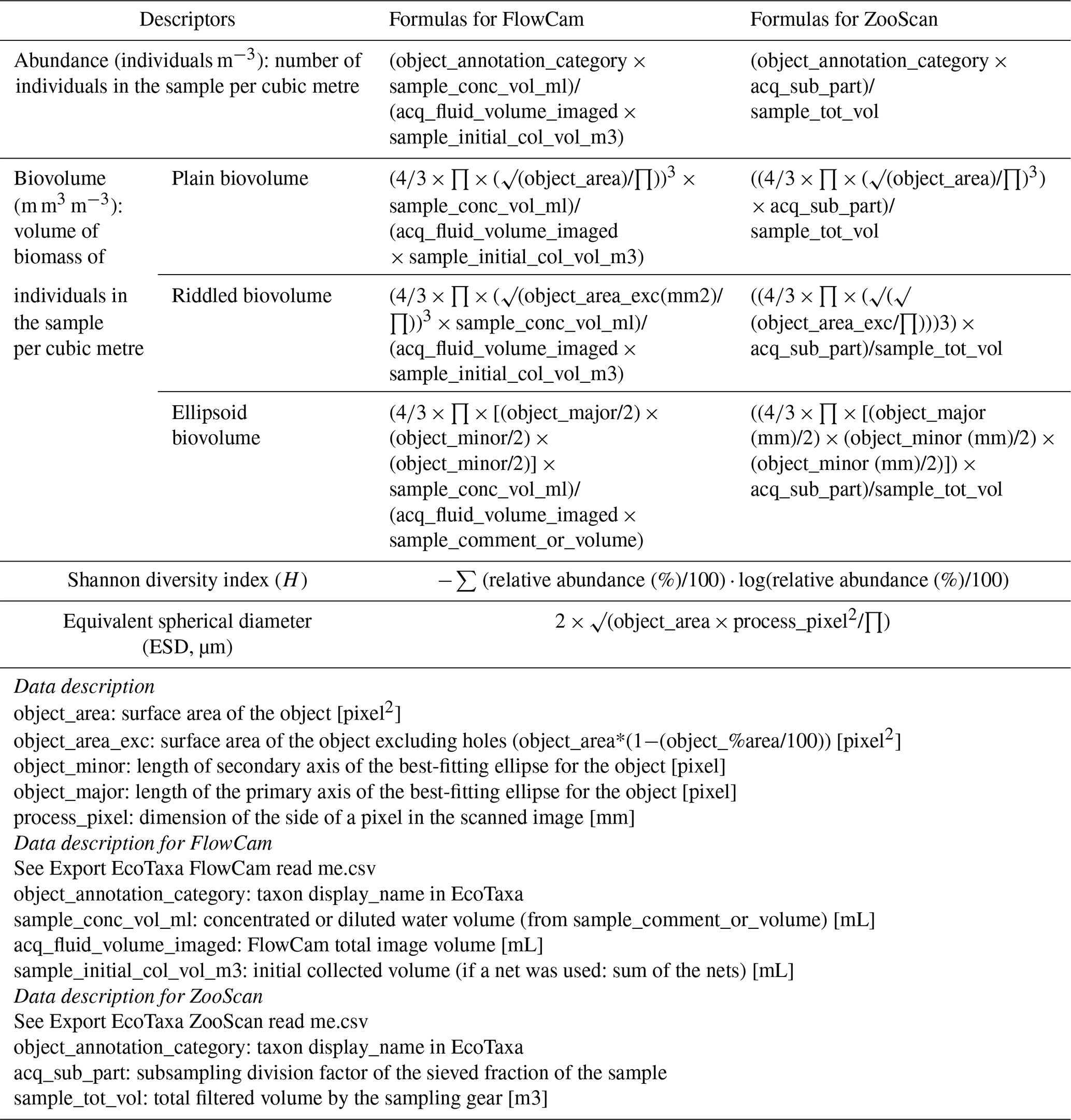
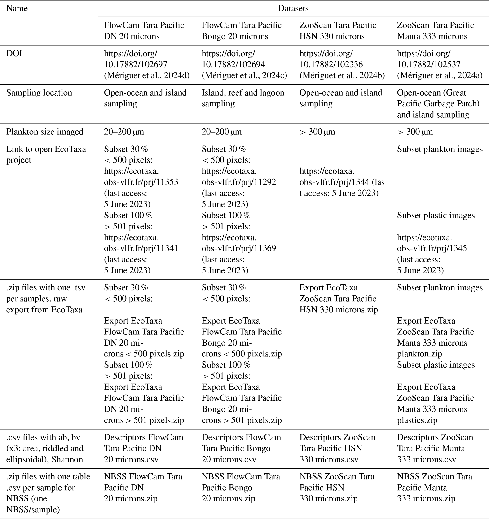
Table 2 Summary of the data availability, description and useful links for each dataset.

3 Technical validation and discussion

3.1 Limitations of bongo net microplankton sampling for quantitative estimations

Both the bongo nets and the DN consisted of a 20 µm mesh to collect surface microplankton throughout the expedition. A key difference between these two nets lies in their deployment locations, which correspond to distinct environments: bongo nets were deployed near islands, reefs or within lagoons, whereas the DN was deployed in the open ocean. These environments are characterised by differing chlorophyll a concentrations, with a clear increase observed near islands and within lagoons, as highlighted in Bourdin et al. (2024). As such, we expected higher plankton concentrations in the reef and lagoon areas and, consequently, in the bongo net samples. However, the majority of bongo net samples showed lower concentrations than nearby open-ocean samples from the DN, as evidenced by the NBSS data (Fig. 5a).

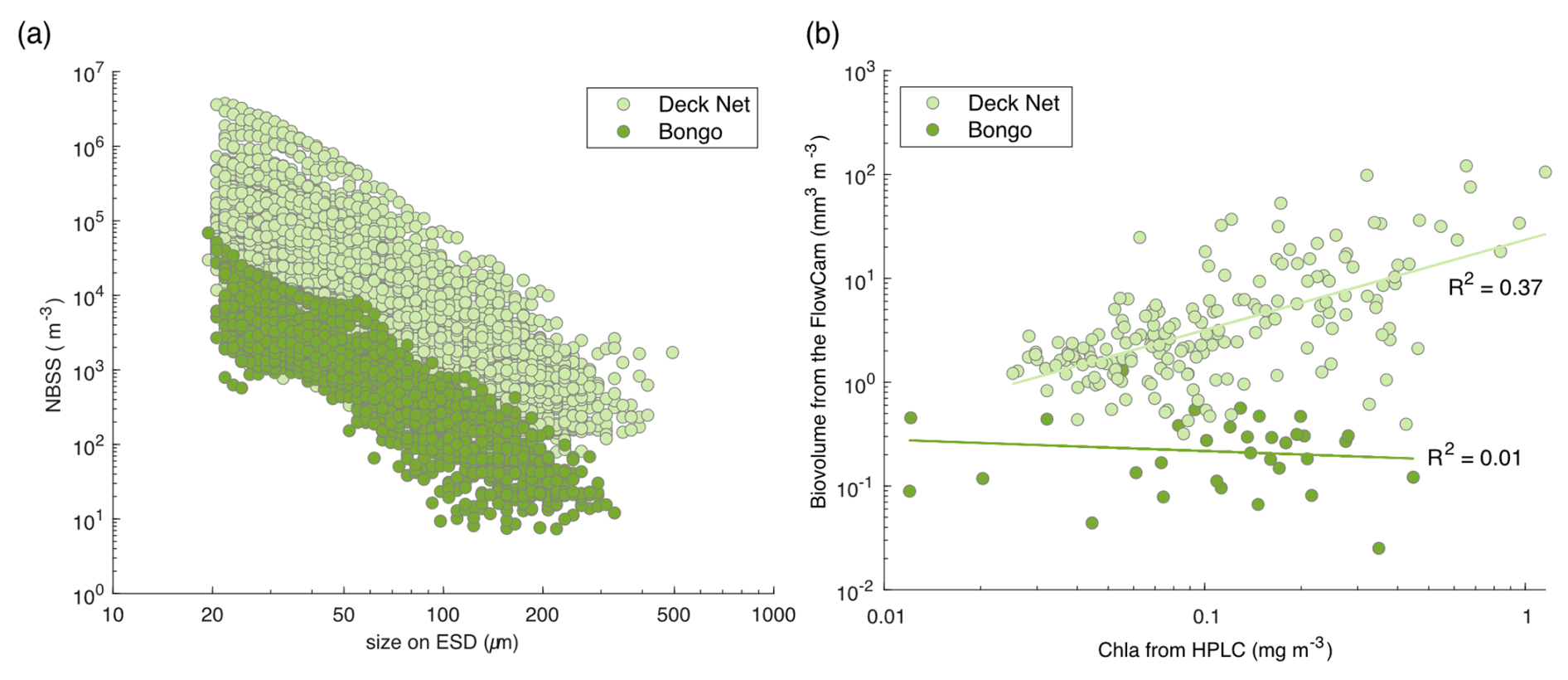
Figure 5 (a) Comparison of normalised biovolume size spectrum (NBSS; in log–log) of the live plankton between the bongo nets (34 samples) and the deck net (207 samples). (b) Phytoplankton biovolume (mm³ m⁻³) estimated from the FlowCam samples, which were collected using the bongo nets and the deck net, according to the chlorophyll a (Chl a) values obtained from the HPLC measurements at the same station. The selection of phytoplankton was made possible by taxonomic validation of FlowCam images from these two nets.

This discrepancy raises concerns about the reliability of the filtered-volume estimates, whether based on flowmeters or theoretical calculations, which are critical for consistent quantitative plankton sampling. Regarding the flowmeters, as mentioned in Sect. 2, bongo nets were equipped with flowmeters rated for speeds above 0.3 m s⁻¹. However, the relatively low towing speed of the underwater scooter was insufficient to generate enough water flow through the 20 µm mesh to reliably rotate the flowmeters. For the theoretical volume, the deployment time of the bongo nets by divers was highly uncertain. The uncertainty surrounding the theoretical volume stemmed from inconsistent deployment times recorded by the divers and methodological biases associated with using an underwater scooter, which made the filtered-volume estimates unreliable. Moreover, the suspended particle concentrations were very variable for different sampling sites, thereby complicating the correct prediction of the towing time required to obtain reasonable concentrate in the net and avoid clogging.

Overall, the lack of correlation of total chlorophyll a and total phytoplankton biovolume from FlowCam, as shown in Fig. 5b, indicates that the bongo net sampling was not quantitative. The chlorophyll a values obtained from the HPLC measurements do not represent the same size classes of phytoplankton as those observed with the FlowCam, but we were interested in whether or not there were likely to be similar trends in phytoplankton biomass changes measured for the same station (Fig. 5b). The correlation between chlorophyll a and total phytoplankton biovolume of the bongo was lower than for the deck net samples. This suggests that phytoplankton biovolume was underestimated relative to chlorophyll a in the bongo samples. Given the methodological limitations of the bongo net filtration volume estimation, our most plausible hypothesis is an overestimation of the theoretical volume, likely due to clogging. Therefore, as a conclusion, it is highly recommended to use bongo net samples for qualitative analysis only.

3.2 Benefits and limitations of high-speed deployment

During the Tara Pacific sampling of open-ocean transects, we decided to take on the challenge of collecting plankton samples while sailing at speeds of up to 9 knots. This high-speed sampling provides valuable opportunities to expand and optimise the coverage of our sampling with a daily frequency. Initially, the Tara Pacific expedition was designed to focus on coral reefs (Planes et al., 2019). The addition of high-speed sampling allowed for the opportunistic use of transit periods, covering a significant spatial area of the expedition. As a result, one of the most valuable aspects of the Tara Pacific plankton samples is the daily collection of samples approximately every 150 to 200 nmi, covering a wide range of oceanic structures across the Pacific Basin. However, it is important to note that, given the patchy spatial distribution of plankton (Robinson et al., 2021), this sampling scale is somehow discrete rather than continuous. This designed sampling is also valuable, as we aimed for “end-to-end” sampling of surface waters (Gorsky et al., 2019) with the micro- to macroplankton fractions presented in this article. However, the constraint of surface sampling and of deploying and retrieving the instruments at cruising speed forced us to develop new, robust, relatively small and user-friendly devices adapted for the Tara schooner. To our knowledge, the combined deployment of the Dolphin system and the high-speed net (HSN), designed for this purpose and presented in this article, represents the first system enabling the discrete sampling of the entire surface planktonic ecosystem with deployment and retrieval at cruising speeds of < 9 knots.

The development of high-speed plankton samplers began in the early 20th century with the well-known Continuous Plankton Recorder (CPR), developed by Alister Hardy in 1926, which was designed to be towed under the surface over long distances at speeds up to 25 knots. Following the CPR, other high-speed net systems emerged, including the Longhurst–Hardy Plankton Recorder (LHPR; Longhurst et al., 1966), the Gulf III OCEAN Sampler (Gehringer, 1958) and the Gulf V plankton sampler (Sameoto et al., 2000), as well as newer low-tech designs (CSN in Von Ammon et al., 2020; Coryphaena in Mériguet et al., 2022). All high-speed zooplankton samplers face the challenge of maintaining filtration efficiency at higher towing speeds. Thus, higher speeds require a larger relative filtration area to optimise filtration efficiency while minimising excessive pressure on the net and mitigating the pressure wave that pushes organisms away from the net (Harris et al., 2000; Keen, 2013; Skjoldal et al., 2013). Therefore, a critical design principle is to obtain a sufficiently high ratio of mesh filtering area to net opening area (Smith and Tranter, 1968; Skjoldal et al., 2013). To achieve this, high-speed zooplankton samplers often employ a small initial opening area that widens internally (e.g. CPR has a 1.27 cm² entrance aperture expanding to 5 cm × 10 cm, while the Gulf V and LHPR use conic noses). This design trade-off, which is essential for pressure reduction, comes at a cost. The small surface area of the mouth opening means a smaller filtered volume, reducing the probability of collecting less abundant, larger organisms (Skjoldal et al., 2013). The avoidance of active-swimming zooplankton, which is dependent on the net opening area size, is also described as the bias affecting the catch of mesoplankton by Harris et al. (2000). This may be discussed, as increasing tow speed may improve the capture efficiency of zooplankton capable of active avoidance (Skjoldal et al., 2013). Therefore, high-speed sampling methods have the advantage of increasing sampling coverage and frequency, but they also introduce bias due to the pressure generated by high speeds, resulting in even greater undersampling compared to traditional nets (Harris et al., 2000; Cook, 2001).

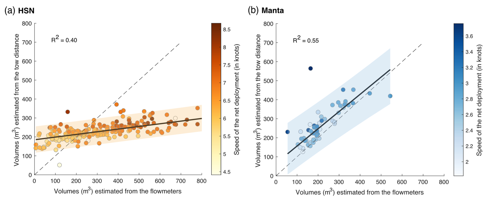
Figure 6 (a, b) Linear regression between volume-filtered estimates from the tow distance (theoric volumes; m³) and estimates from the flowmeters for the respective HSN and manta net samples. The range of the 95 % confidence intervals is represented in orange for the HSN and in blue for the manta net. The 1:1 dotted line represents the linear regression obtained if both volumes were similar. The colour of the dots represents the deployment speed of the net (in knots).

3.2.1 Impact on filtered-volume estimation

One of the primary challenges in quantitative plankton sampling is the estimation of the filtered volume. Because the immersion depth of surface nets changes constantly with waves, wind and boat movement, it is difficult to accurately calculate the volume of water being filtered (see the review in Pasquier et al., 2022). Results obtained by different studies show that a surface sampling with a difference in immersion depth of a few centimetres can lead to a large difference in the sampled volume (Pasquier et al., 2022). Overall, the impact of high-speed deployment on the filtered volume remains largely unexplored in the literature with the exception of Jonas (2004). The aforementioned work tested the relationship between the CPR filtered volumes estimated by a flowmeter or by theory and their relationship with the CPR deployment speed. The findings revealed overestimations by the flowmeter compared to theoretical values. This raises concerns about the effectiveness of flowmeters with respect to measuring volumes during high-speed deployments. Therefore, we investigated whether our high-speed surface sampling approach had an effect on the filtered-volume measurements.

For the DN, the water intake was identical to the HSN with respect to the design and mouth opening, but a flowmeter was integrated into the water circuit downstream of the pump and two de-bubblers were added (see Fig. 6 in Gorsky et al., 2019). This allowed for reliable estimation of water volumes that were pumped into the DN based on flowmeter recordings (Gorsky et al., 2019). Both the HSN and manta net were equipped with mechanical flowmeters mounted in the inlet frame, while the towed distance, time and speed were recorded aboard the ship to estimate the theoretical volume filtered. While the HSN was towed at between 3.9 and 9 knots, the manta net was towed at a lower speed of between 1.2 knots and (a maximum speed of) 3.6 knots (Fig. 6).

Figure 6 shows a clear discrepancies in the slope of the estimated volumes between the HSN and the manta net, meaning that the theoretical and flowmeter filtered volumes of the manta net are closer to each other than for the HSN. Manta net theoretical volumes tend to be higher and, thus, potentially overestimated compared to flowmeter measurements (Fig. 6b), but the difference remains generally small compared to the HSN. For the HSN, flowmeter estimation methods provide volumes of the same order of magnitude as the theoretical volume for the HSN, although the values exhibit considerable differences between stations (mean difference between the flowmeter and theoretical volumes per station is 90.5 with a standard deviation of 172.6; Fig. 6a). Linear regression analysis between these volume differences per station (flowmeter–theoretical volume) and speed deployment showed a significant relationship, with a slope coefficient of 91.168 (standard deviation = 11.86, t test = 7.69 and p value < 0.001), indicating that higher speeds are associated with greater differences. Consistently with the results of Jonas (2004) described before, the high-speed deployment is, thus, associated with the overestimation of the flowmeter volumes compared to theoretical ones (Fig. 6a). These results indicate that the use of the flowmeters is not appropriate under high-speed conditions. The pressure increase caused by a high speed generates turbulence and could affect the flowmeter rotation and explain the overestimation of the filtered volume that we found for high speeds. Globally, the turbulence generated could explain the malfunction of flowmeters, which are designed and calibrated by the manufactures to accurately measure flow speed in a laminar flow. This result is highlighted by Skjoldal et al. (2019), who assumed that the use of flowmeters was complicated by their position in relation to the cross-sectional flow field or their functioning in a turbulent system.

In addition to the speed, we tested if the HSN's immersion depth varied when the sea state was high. The HSN was designed to sample the surface ocean, at the air–seawater interface; thus, the upper part of its mouth opening was rarely completely submerged during deployment (see images in Fig. 4 in Gorsky et al., 2019). The relationships between wind strength (as a proxy for sea state) recorded by Tara's navigation instruments and the two estimates of HSN sampling volumes showed no correlation (R²=0.00 for flowmeter volumes and for theoretical volumes; data not shown). While the flowmeter does not provide accurate flow measurements under turbulent conditions, it appears that the sea state does not affect its volume estimates.

Therefore, we recommended using the theoretical volume for the HSN. The towing distance used is relative to the ground, not to the seawater; therefore, there is a potential bias in the theoretical volume estimation due to the non-consideration of the surface current speed. This bias is likely negligible for the majority of our samples located in the subtropical gyres, mostly characterised by relatively low geostrophic currents (Tara Pacific data available from Bourdin et al., 2022, in “at current_speed_copernicus”).

3.2.2 Quantitative comparison between the HSN and manta net

The manta net was designed to study neuston and floating particles, such as microplastics. Thus, it is the most commonly used net for studying surface plankton and is widely recognised as a reference system for investigating the surface ocean (Eriksen et al., 2018; Karlsson et al., 2020; Pasquier et al., 2022). Both the HSN and the manta net were deployed at the same stations when approaching islands and in the Great Pacific Garbage Patch. The manta net was deployed in closer proximity to islands than the HSN. Given that the HSN was towed for a duration of 60–90 min, whereas the manta net was towed for approximately 30–40 min, the decision was made to sample with the manta net in the immediate vicinity of the island, in order to capture the variability associated with the island mass effect.

We conducted a comparison of the normalised biovolume size spectrum (NBSS; Fig. 7a) obtained from the two nets. The analysis follows the work presented in Lombard et al. (2023), incorporating data from 31 additional samples collected by the HSN. The NBSS of both nets was of the same order of magnitude, with manta biovolumes appearing to be higher in each NBSS size class (Fig. 7a), suggesting an underestimation by the HSN. Considering the principle that, when represented on a logarithmic scale (as in Fig. 7c), the intercept of the NBSS data reflects the total abundance of organisms in the studied ecosystem (Platt and Denman, 1978) and assuming that the same water masses were sampled, we compared the NBSS intercepts, which support the underestimation by the HSN, as higher intercepts were observed for the manta (with the NBSS intercept of the HSN showing 0.2 compared to 0.8 for the manta). This difference was expected due to the undersampling at high speed compared to traditional plankton sampling discussed above. In contrast to the HSN, which has a smaller mouth opening, leading to a smaller sampling volume, the manta net benefits from a larger opening and lower towing speed. This combination reduces turbulence and allows for a larger sampling volume, resulting in potentially lower loss. This is reflected in Fig. 7a, where the manta net captures a wider range of sizes, including larger and rarer fragile organisms. Skjoldal et al. (2019) measured less biomass in the large size fraction and more biomass in the small and medium size fractions at higher towing speeds. The opposite effect might have been expected for the small fraction due to extrusion (Skjoldal et al., 2019), suggesting that the HSN may be more effective at capturing smaller organisms. However, this is not clearly demonstrated, as the slopes of the HSN's NBSS data are largely equivalent to those of the manta (mean NBSS slope for HSN = −0.35, SD = 0.30, and mean NBSS slope for manta = −0.30, SD = 0.23; Fig. 7a). This also suggests that both nets capture the same trophic plankton ecosystem structure, although the HSN underestimates plankton in each size class.

Figure 7 (a) Comparison of normalised biovolume size spectrum (NBSS) data of living organisms sampled with the HSN (yellow dots) and manta net (blue dots). Only stations where both were deployed are included in this figure. The average taxonomic composition of the “plankton groups” with respect to biovolume (mm³ m⁻³) for all stations by size class (in µm) for samples collected with the (b) HSN and (c) manta net.

All of these observed differences may, therefore, introduce differences in species composition. Investigating the taxonomic composition, the HSN and the manta net show, on average, relatively similar community compositions (the dinoflagellates are almost entirely composed of the genus Noctiluca; Fig. 7c and d). Investigating the taxonomic composition in terms of biovolume, the five most represented groups in the manta dataset are Cnidaria (59 %), Copepoda (13 %), other (11 %), Crustacea (9 %) and Mollusca (3 %). In contrast, the HSN dataset shows a more even distribution, with other taxa contributing 33 %, followed by Cnidaria (28 %), Copepoda (19 %), Tunicata (10 %) and Crustacea (6 %). Although there is a general difference in the sampled plankton community, the greatest discrepancies are observed for gelatinous organisms. Thus, the HSN undersampled larger and more fragile organisms such as cnidarians and tunicates (Fig. 7c). This aligns with the limitations of high-speed deployments, which have been shown to damage delicate organisms (Harris et al., 2000; Keen, 2013). This damage to large and fragile plankton could cause the higher concentrations of smaller size classes that we found in the HSN compared to the manta net samples. In contrast, the HSN consistently sampled more robust organisms such as copepods and chaetognaths than the manta net (Figs. 7c and 6d).

For the quantitative and qualitative comparison of plankton community sampling, we only considered stations where both nets were deployed sequentially (first the manta net and then the HSN). Although small, this temporal and spatial difference remains a limitation in our comparison between the two nets. In terms of location, this combination of manta–HSN deployments was primarily conducted near islands, where plankton concentrations and composition are known to be highly variable (Bourdin et al., 2024; Kristan et al., in prep). Given that the manta net was deployed before the HSN, i.e. closer to the islands, we also expect part of the HSN underestimation signal to be explained by this small spatial difference. Therefore, while our primary hypothesis mainly attributes these differences to the high-speed deployment of the HSN (up to 3 times greater than that of the manta), these spatial and temporal factors, in addition to the patchiness distribution of plankton (Robinson et al., 2021), may also play a role in our comparison of the two plankton sampling systems.

4 General discussion

In conclusion to our investigation of sampling biases associated with the high-speed sampling, the HSN must be considered to be semi-quantitative. The use of the HSN introduces an undersampling bias that is also found in other high-speed samplers, as described for the CPR. Nevertheless, we highlight the usefulness of the HSN for (1) sampling surface zooplankton when it is not possible to stop or slow the boat and (2) extending sampling coverage and frequency. Consistent with the CPR, the HSN captures a roughly consistent fraction of the in situ abundance, reflecting the main patterns observed in plankton. Consistent with expected ecological trends, higher plankton abundances and biovolumes are observed in nutrient-rich regions such as coastal and upwellings, whereas oligotrophic gyres exhibit significantly lower biomass (see abundance, biovolume and diversity maps for each sampling device in Appendix B). For example, the trend of increasing plankton abundance due to California upwelling (Checkley and Barth, 2009) appears to emerge regardless of the sampling method used (Figs. B1–B4). Each net is a filter through which we sample the ocean, but if the overall patterns they show are consistent, we can conclude that they are likely to be robust patterns. This is true for many types of sampling nets, as many previous studies have shown (Herdman, 1921; Barnes and Marshall, 1951; Anraku, 1956; Wiebe and Holland, 1968).

In addition to the unique characteristic of high-speed sampling, these datasets are also distinguished by their focus on surface plankton communities during daytime, offering both advantages and limitations. These surface plankton data enrich interdisciplinary studies of the ocean's surface layer, in direct association with other surface measurements (satellite and atmospheric data; Lombard et al., 2019). This surface ecosystem, hosting a uniquely diverse planktonic community, remains largely unexplored, but it appears to play an essential role in ocean–climate feedbacks (Helm, 2021; Hunter, 2023), acting as a critical interface between atmospheric and oceanic process and contributing significantly to biogeochemical cycles (Falkowski et al., 2008). Processes controlling the abundance and diversity of the surface plankton communities may be significantly different from those in deeper layers (Ibarbalz et al., 2019; Santiago et al., 2023). The surface is also on the front line of climate change and pollution. Thus, these particular communities face increasing challenges such as rising temperatures, stratification and nutrient stress (Bopp et al., 2013; IPCC, 2023), and floating contaminants (e.g. plastics, metals and toxins, and petroleum) (Helm, 2021). However, surface plankton sampling has limitations regarding the “quantitative representativeness” of the broader plankton ecosystem in the water column. The Tara Pacific sampling was conducted under stable daytime conditions, minimising variability from diel vertical migration (Lampert, 1989). As a result, zooplankton concentrations do not reflect deeper-dwelling organisms, particularly those migrating to the surface at night, leading to potentially higher abundances within the water column (Lampert, 1989). This is also valuable for phytoplankton communities that are known to be heterogeneously distributed from the surface to deeper waters into the euphotic zone, especially in the transparent oligotrophic waters of the Pacific gyre, where deep chlorophyll maxima can occur tens to hundreds of metres below the surface (Mignot et al., 2014). In terms of comparison with non-surface plankton data, this limitation must be carefully considered by future users.

5 Data availability

The referenced datasets related to the figures are available from the following sources: https://doi.org/10.17882/102537 (Mériguet et al., 2024a) (EcoTaxa link: https://ecotaxa.obs-vlfr.fr/prj/1344, Pedrotti et al., 2025a and https://ecotaxa.obs-vlfr.fr/prj/1345, Pedrotti et al., 2025b), https://doi.org/10.17882/102336 (Mériguet et al., 2024b) (EcoTaxa link: https://ecotaxa.obs-vlfr.fr/prj/11292, Mériguet and Lombard, 2025a), https://doi.org/10.17882/102694 (Mériguet et al., 2024c) (EcoTaxa link: https://ecotaxa.obs-vlfr.fr/prj/11370, Mériguet et al., 2025a and https://ecotaxa.obs-vlfr.fr/prj/11369, Mériguet et al., 2025b) and https://doi.org/10.17882/102697 (Mériguet et al., 2024d) (EcoTaxa link: https://ecotaxa.obs-vlfr.fr/prj/11353, Mériguet and Lombard, 2025b and https://ecotaxa.obs-vlfr.fr/prj/11341, Mériguet and Lombard, 2025c).

The imaging datasets are also summarised in Table 2. A key strength of the quantitative imaging datasets is their complementarity, with a wide range of environmental data collected during the Tara Pacific expedition. This expedition is described in detail in Lombard et al. (2023), where the full set of environmental datasets are available and referenced: https://doi.org/10.1038/s41597-022-01757-w. Environmental data were collected on a station-by-station basis, making it possible to link them directly to our dataset using the station name. Each station is identified by a unique [oa###] code, where the “oa” label is the key identifier for associating the environmental measurements with our imaging data. When looking at data at this “station” level, all environmental data are already compiled and compatible for easy analysis and cross-analysis, and when linked to sample barcodes, they could be further linked to any other associated data (e.g. genomic) by linking them to the sample registry available in Lombard et al. (2023), with the sample and event registry being available at https://doi.org/10.5281/ZENODO.6474974 (Bourdin et al., 2022). In addition to station-based data, continuous environmental measurements from the Tara Pacific expedition (Lombard et al., 2023) can also be linked to our dataset. These measurements can be linked to plankton net sampling events using the date, time and GPS coordinates, all of which are available in both the plankton and in-line environmental datasets. This ensures a robust integration of imaging and environmental data, facilitating large-scale ecological analyses.

6 Conclusion

The Tara Pacific expedition is part of the first initiatives aiming to implement a system for discrete sampling of the planktonic ecosystem while operating at cruising speed (5–9 knots), covering viruses to metazoa at the expedition scale (Gorsky et al., 2019) and focusing on micro- to mesoplankton in this paper. The use of two new sampling systems highlights some biases that lead to undersampling, which is important to consider in subsequent ecological analyses. However, the simultaneous high-speed sampling of the different components of the surface ecosystem may contribute to addressing the issue of undersampling of the open ocean at difficult-to-reach spatial and temporal scales, which is a major challenge for marine science. These systems can be improved and adapted to vessels of different sizes and with propulsion systems, opening the way to complementary initiatives, such as plankton collection by citizen sailors (De Vargas et al., 2022; Mériguet et al., 2022).

In conclusion, using these new sampling methods covering the North and South Pacific and North Atlantic basins, we provide an important dataset focusing on the surface plankton rarely sampled as a whole. Our large-scale analysis reveals an important taxonomic and functional diversity within the surface planktonic communities, encompassing approximately 370 different taxa, primarily identified at the genus level, spanning across 12 major plankton groups and 5 trophic levels. We hope that the dataset presented here, will stimulate further studies (e.g. biodiversity, biogeochemistry and modelling studies) using the different environmental imprints recorded during the Tara Pacific expedition (data available in Lombard et al., 2023) to highlight the processes influencing this particular plankton ecosystem, from large-scale to mesoscale levels, from the taxonomic to trophic scale or from species barcodes to genomes. Such an important dataset will not only serve as a starting point for many studies to deepen our understanding of planktonic ecosystems, their biogeochemical roles and their socio-economic importance but could also serve as a reference state of the ecosystem in the context of environmental changes.

Appendix A

Table A1 List of EcoTaxa taxonomic annotations and associated groups: plankton group and trophic type for the FlowCam DN 20 microns dataset.

Table A2 List of EcoTaxa taxonomic annotations and associated groups: plankton group and trophic type for the FlowCam Bongo 20 microns dataset.

Table A3 List of EcoTaxa taxonomic annotations and associated groups: plankton group and trophic type for the ZooScan HSN 330 microns dataset.

Table A4 List of EcoTaxa taxonomic annotations and associated groups: plankton group and trophic type for the ZooScan Manta 333 microns dataset.

Appendix B

Figure B1 FlowCam DN 20 microns: (a) map of the plankton abundance (individuals m⁻³); (b) map of the plankton biovolume (mm m⁻³); (c) map of the Shannon diversity index.

Figure B2 FlowCam Bongo 20 microns: (a) map of the plankton abundance (individuals m⁻³); (b) map of the plankton biovolume (mm m⁻³); (c) map of the Shannon diversity index.

Figure B3 ZooScan HSN 330 microns: (a) map of the plankton abundance (individuals m⁻³); (b) map of the plankton biovolume (mm m⁻³); (c) map of the Shannon diversity index.

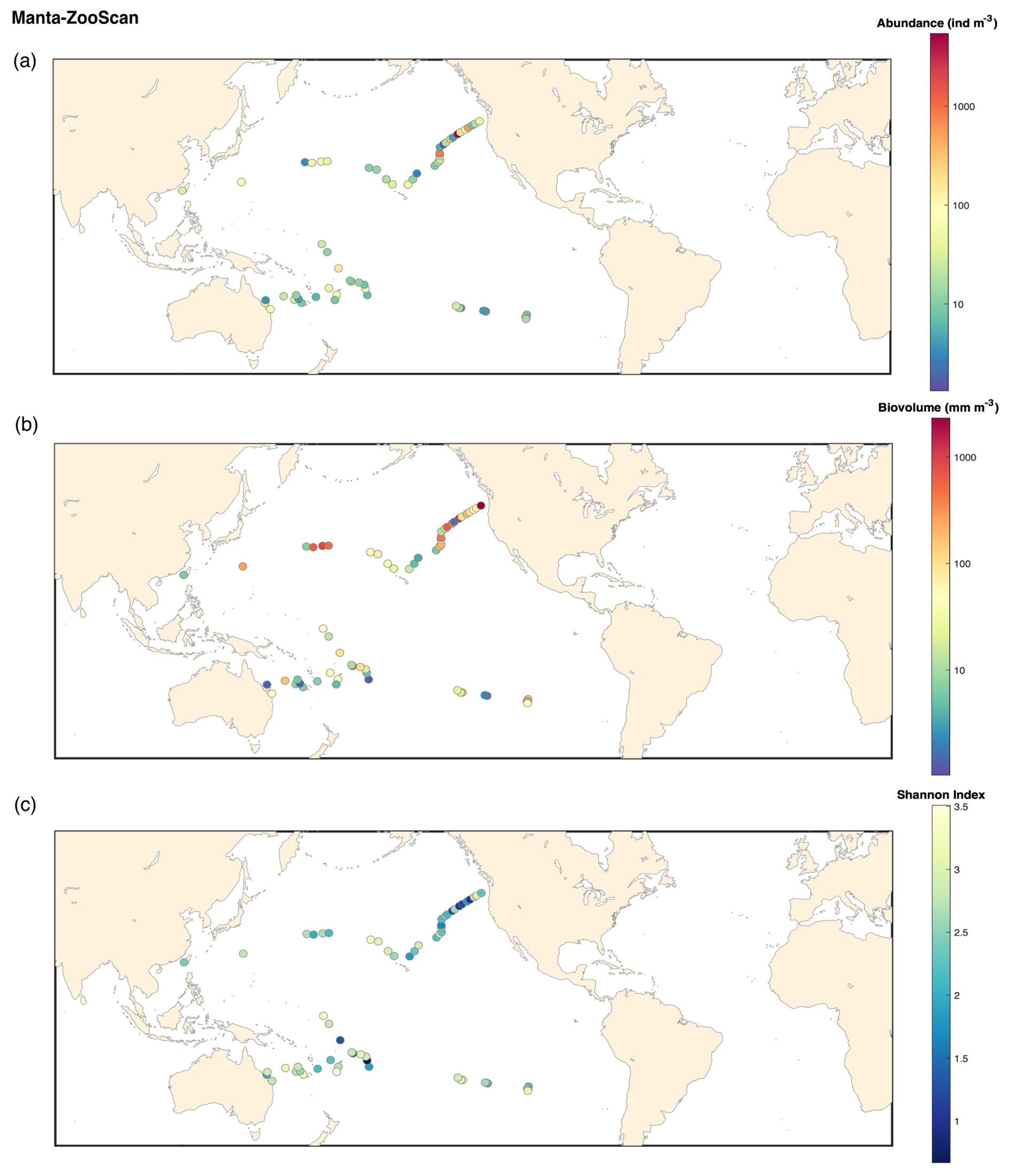
Figure B4 ZooScan Manta 333 microns: (a) map of the plankton abundance (individuals m⁻³); (b) map of the plankton biovolume (mm m⁻³); (c) map of the Shannon diversity index.

Appendix C

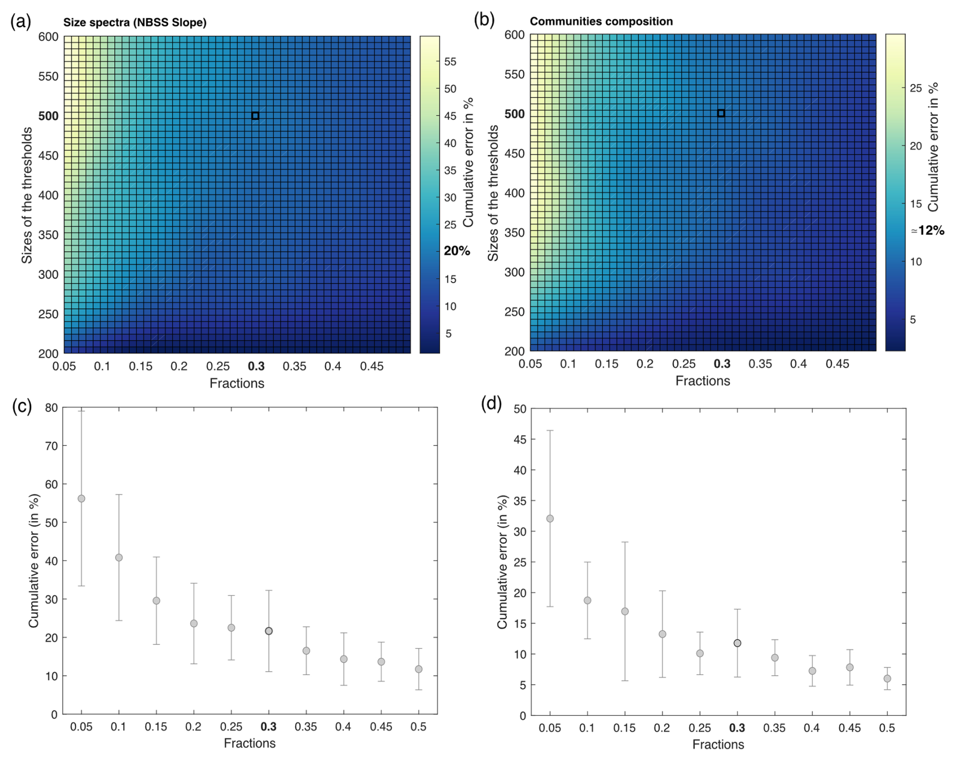
Figure C1 (a, b) Estimated cumulative error associated with partial validation of particles below a size cut-off threshold ranging from 200 to 600 pixels and validated fractions ranging from 5 % to 50 %. Errors are computed as the percentage root-mean-square error (RMSE) between fully validated samples and partially validated samples using three different metrics for cumulative error in the NBSS slope and community composition (relative abundance), respectively. RMSE values represent the outcomes of simulations, each conducted three times for the four samples, with random sampling. (c, d) Cumulative error according to the fractions chosen in the NBSS slope and community composition, respectively. The threshold is fixed at 500 pixels.