the Creative Commons Attribution 4.0 License.
the Creative Commons Attribution 4.0 License.
 | 09 May 2025
Global Methane Budget 2000–2020
Marielle Saunois
Adrien Martinez
Benjamin Poulter
Zhen Zhang
Peter A. Raymond
Pierre Regnier
Josep G. Canadell
Robert B. Jackson
Prabir K. Patra
Philippe Bousquet
Philippe Ciais
Edward J. Dlugokencky
George H. Allen
David Bastviken
David J. Beerling
Dmitry A. Belikov
Donald R. Blake
Simona Castaldi
Monica Crippa
Bridget R. Deemer
Fraser Dennison
Giuseppe Etiope
Nicola Gedney
Lena Höglund-Isaksson
Meredith A. Holgerson
Peter O. Hopcroft
Gustaf Hugelius
Akihiko Ito
Atul K. Jain
Rajesh Janardanan
Matthew S. Johnson
Thomas Kleinen
Paul B. Krummel
Ronny Lauerwald
Tingting Li
Xiangyu Liu
Kyle C. McDonald
Joe R. Melton
Jens Mühle
Jurek Müller
Fabiola Murguia-Flores
Yosuke Niwa
Sergio Noce
Shufen Pan
Robert J. Parker
Changhui Peng
Michel Ramonet
William J. Riley
Gerard Rocher-Ros
Judith A. Rosentreter
Motoki Sasakawa
Arjo Segers
Steven J. Smith
Emily H. Stanley
Joël Thanwerdas
Hanqin Tian
Aki Tsuruta
Francesco N. Tubiello
Thomas S. Weber
Guido R. van der Werf
Douglas E. J. Worthy
Yukio Yoshida
Wenxin Zhang
Qing Zhu
Qiuan Zhu
Qianlai Zhuang
Understanding and quantifying the global methane (CH4) budget is important for assessing realistic pathways to mitigate climate change. CH4 is the second most important human-influenced greenhouse gas in terms of climate forcing after carbon dioxide (CO2), and both emissions and atmospheric concentrations of CH4 have continued to increase since 2007 after a temporary pause. The relative importance of CH4 emissions compared to those of CO2 for temperature change is related to its shorter atmospheric lifetime, stronger radiative effect, and acceleration in atmospheric growth rate over the past decade, the causes of which are still debated. Two major challenges in quantifying the factors responsible for the observed atmospheric growth rate arise from diverse, geographically overlapping CH4 sources and from the uncertain magnitude and temporal change in the destruction of CH4 by short-lived and highly variable hydroxyl radicals (OH). To address these challenges, we have established a consortium of multidisciplinary scientists under the umbrella of the Global Carbon Project to improve, synthesise, and update the global CH4 budget regularly and to stimulate new research on the methane cycle. Following Saunois et al. (2016, 2020), we present here the third version of the living review paper dedicated to the decadal CH4 budget, integrating results of top-down CH4 emission estimates (based on in situ and Greenhouse Gases Observing SATellite (GOSAT) atmospheric observations and an ensemble of atmospheric inverse-model results) and bottom-up estimates (based on process-based models for estimating land surface emissions and atmospheric chemistry, inventories of anthropogenic emissions, and data-driven extrapolations). We present a budget for the most recent 2010–2019 calendar decade (the latest period for which full data sets are available), for the previous decade of 2000–2009 and for the year 2020.
The revision of the bottom-up budget in this 2025 edition benefits from important progress in estimating inland freshwater emissions, with better counting of emissions from lakes and ponds, reservoirs, and streams and rivers. This budget also reduces double counting across freshwater and wetland emissions and, for the first time, includes an estimate of the potential double counting that may exist (average of 23 Tg CH4 yr−1). Bottom-up approaches show that the combined wetland and inland freshwater emissions average 248 [159–369] Tg CH4 yr−1 for the 2010–2019 decade. Natural fluxes are perturbed by human activities through climate, eutrophication, and land use. In this budget, we also estimate, for the first time, this anthropogenic component contributing to wetland and inland freshwater emissions. Newly available gridded products also allowed us to derive an almost complete latitudinal and regional budget based on bottom-up approaches.
For the 2010–2019 decade, global CH4 emissions are estimated by atmospheric inversions (top-down) to be 575 Tg CH4 yr−1 (range 553–586, corresponding to the minimum and maximum estimates of the model ensemble). Of this amount, 369 Tg CH4 yr−1 or ∼ 65 % is attributed to direct anthropogenic sources in the fossil, agriculture, and waste and anthropogenic biomass burning (range 350–391 Tg CH4 yr−1 or 63 %–68 %). For the 2000–2009 period, the atmospheric inversions give a slightly lower total emission than for 2010–2019, by 32 Tg CH4 yr−1 (range 9–40). The 2020 emission rate is the highest of the period and reaches 608 Tg CH4 yr−1 (range 581–627), which is 12 % higher than the average emissions in the 2000s. Since 2012, global direct anthropogenic CH4 emission trends have been tracking scenarios that assume no or minimal climate mitigation policies proposed by the Intergovernmental Panel on Climate Change (shared socio-economic pathways SSP5 and SSP3). Bottom-up methods suggest 16 % (94 Tg CH4 yr−1) larger global emissions (669 Tg CH4 yr−1, range 512–849) than top-down inversion methods for the 2010–2019 period. The discrepancy between the bottom-up and the top-down budgets has been greatly reduced compared to the previous differences (167 and 156 Tg CH4 yr−1 in Saunois et al. (2016, 2020) respectively), and for the first time uncertainties in bottom-up and top-down budgets overlap. Although differences have been reduced between inversions and bottom-up, the most important source of uncertainty in the global CH4 budget is still attributable to natural emissions, especially those from wetlands and inland freshwaters.
The tropospheric loss of methane, as the main contributor to methane lifetime, has been estimated at 563 [510–663] Tg CH4 yr−1 based on chemistry–climate models. These values are slightly larger than for 2000–2009 due to the impact of the rise in atmospheric methane and remaining large uncertainty (∼ 25 %). The total sink of CH4 is estimated at 633 [507–796] Tg CH4 yr−1 by the bottom-up approaches and at 554 [550–567] Tg CH4 yr−1 by top-down approaches. However, most of the top-down models use the same OH distribution, which introduces less uncertainty to the global budget than is likely justified.
For 2010–2019, agriculture and waste contributed an estimated 228 [213–242] Tg CH4 yr−1 in the top-down budget and 211 [195–231] Tg CH4 yr−1 in the bottom-up budget. Fossil fuel emissions contributed 115 [100–124] Tg CH4 yr−1 in the top-down budget and 120 [117–125] Tg CH4 yr−1 in the bottom-up budget. Biomass and biofuel burning contributed 27 [26–27] Tg CH4 yr−1 in the top-down budget and 28 [21–39] Tg CH4 yr−1 in the bottom-up budget.
We identify five major priorities for improving the CH4 budget: (i) producing a global, high-resolution map of water-saturated soils and inundated areas emitting CH4 based on a robust classification of different types of emitting ecosystems; (ii) further development of process-based models for inland-water emissions; (iii) intensification of CH4 observations at local (e.g. FLUXNET-CH4 measurements, urban-scale monitoring, satellite imagery with pointing capabilities) to regional scales (surface networks and global remote sensing measurements from satellites) to constrain both bottom-up models and atmospheric inversions; (iv) improvements of transport models and the representation of photochemical sinks in top-down inversions; and (v) integration of 3D variational inversion systems using isotopic and/or co-emitted species such as ethane as well as information in the bottom-up inventories on anthropogenic super-emitters detected by remote sensing (mainly oil and gas sector but also coal, agriculture, and landfills) to improve source partitioning.
The data presented here can be downloaded from https://doi.org/10.18160/GKQ9-2RHT (Martinez et al., 2024).
- Article
(4698 KB) - Full-text XML
-
Supplement
(3298 KB) - BibTeX
- EndNote


The average surface dry air mole fraction of atmospheric methane (CH4) reached 1912 ppb in 2022 (Fig. 1; Lan et al., 2024), 2.6 times greater than its estimated pre-industrial value in 1750. This increase is attributable in large part to increased anthropogenic emissions arising primarily from agriculture (e.g. livestock production, rice cultivation, biomass burning), fossil fuel production and use, waste disposal, and alterations to natural CH4 fluxes due to increased atmospheric CO2 concentrations, land use (Woodward et al., 2010, Fluet-Chouinard et al., 2023), and climate change (Ciais et al., 2013; Canadell et al., 2021). An equal mass of CH4 emissions has a stronger impact on climate than carbon dioxide (CO2), which is reflected by its global warming potential (GWP) relative to CO2 on a given time horizon. For a 100-year time horizon the GWP of CH4 emitted by fossil sources is 29.8 (GWP of CH4 emitted by microbial sources is 27), whereas the values reach 82.5 over a 20-year horizon for CH4 emitted by fossil sources and 79.7 for CH4 emitted by microbial sources (Forster et al., 2021). Although global anthropogenic emissions of CH4 are estimated at around 359 Tg CH4 yr−1 (Saunois et al., 2020), representing around 2.5 % of the global CO2 anthropogenic emissions when converted to units of carbon mass flux for the recent decade, the emissions-based effective radiative forcing of CH4 concentrations contributed ∼ 31 % (1.19 W m−2) to the additional radiative forcing from anthropogenic emissions of greenhouse gases and their precursors (3.84 W m−2) over the industrial era (1750–2019) (Forster et al., 2021). Changes in other chemical compounds such as nitrogen oxides (NOx) or carbon monoxide (CO) also influence atmospheric CH4 through changes to its atmospheric lifetime. Emissions of CH4 contribute to the production of ozone, stratospheric water vapour, and CO2, and most importantly they affect its own lifetime (Myhre et al., 2013; Shindell et al., 2012). CH4 has a short lifetime in the atmosphere (about 9 years for the year 2010; Prather et al., 2012; Szopa et al., 2021). Hence a stabilisation or reduction of CH4 emissions leads to the stabilisation or reduction of its atmospheric concentration (assuming no change in the chemical oxidants), and therefore its radiative forcing, in only a few decades. While reducing CO2 emissions is necessary to stabilise long-term warming, reducing CH4 emissions is recognised as an effective option to limit climate warming in the near-term future (Shindell et al., 2012; Jackson et al., 2020; Ocko et al., 2021; UNEP, 2021) because of its shorter lifetime compared to CO2.
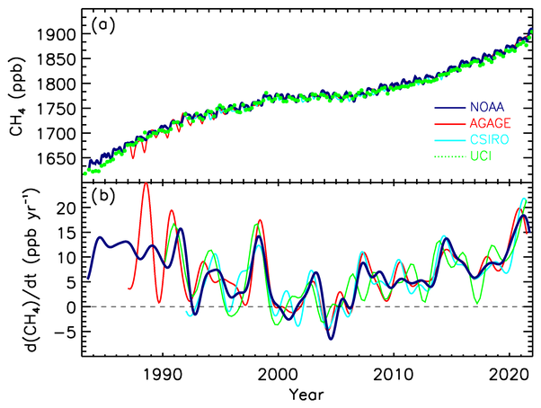
Figure 1Globally averaged atmospheric CH4 concentrations (ppb) (a) and annual growth rates GATM (ppb yr−1) (b) between 1983 and 2022, from four measurement programmes: National Oceanic and Atmospheric Administration (NOAA), Advanced Global Atmospheric Gases Experiment (AGAGE), Commonwealth Scientific and Industrial Research Organisation (CSIRO), and University of California, Irvine (UCI). Detailed descriptions of methods are given in the supplementary material of Kirschke et al. (2013).
The momentum around the potential of CH4 to limit near-term warming led to the launch of the Global Methane Pledge at the November 2021 Conference of the Parties (COP 26). Signed by 158 countries (update on October 2024), this collective effort aims at reducing global CH4 anthropogenic emissions by at least 30 % from 2020 levels by 2030 (Global Methane Pledge, 2023). Given that global baseline CH4 emissions are expected to grow through 2030 (by an additional 20–50 Mt of CH4, UNEP, 2022), the CH4 emission reductions currently needed to reach the Global Methane Pledge objective (UNEP, 2022) correspond to 36 % of the projected baseline emissions in 2030 (i.e. if no further emission reductions were implemented). This implies that large reductions of CH4 emissions are needed to meet the Global Methane Pledge, which is also consistent with the 1.5–2 °C target of the Paris Agreement (UNEP, 2022). Moreover, because CH4 is a precursor of important air pollutants such as ozone, CH4 emissions reductions are required by two international conventions – the United Nations Framework Convention on Climate Change (UNFCCC) and the Convention on Long-Range Transport of Air Pollution (CLRTAP) – making this global CH4 budget assessment all the more critical.
Changes in the magnitude and temporal variation (annual to interannual) in CH4 sources and sinks over the past decades are characterised by large uncertainties (e.g. Kirschke et al., 2013; Saunois et al., 2017; Turner et al., 2019). Also, the decadal budget suggests relative uncertainties (hereafter reported as min–max ranges) of 20 %–35 % for inventories of anthropogenic emissions in specific sectors (e.g. agriculture, waste, fossil fuels; Tibrewal et al., 2024), 50 % for biomass burning and natural wetland emissions, and up to 100 % for other natural sources (e.g. inland waters, geological sources). The uncertainty in the chemical loss of CH4 by OH, the predominant sink of atmospheric CH4, has been estimated using Prather et al. (2012) and Rigby et al. (2017). The former study estimated this uncertainty at ∼ 10 % from the uncertainty in the reaction rate between CH4 and OH, and the latter study was based on methyl-chloroform measurements. Bottom-up approaches (chemistry transport models) estimate the uncertainty of the chemical loss by OH at around 15 %–20 % (Saunois et al., 2016, 2020). This uncertainty in the OH-induced loss translates, in the top-down methods, into the minimum relative uncertainty associated with global CH4 emissions, as other CH4 sinks (atomic oxygen and chlorine oxidations, soil uptake) are much smaller and the atmospheric growth rate is well defined (Dlugokencky et al., 2009). Globally, the contribution of natural CH4 emissions to total emissions can be quantified by combining lifetime estimates with reconstructed pre-industrial atmospheric CH4 concentrations from ice cores (assuming natural emissions have not been perturbed during the Anthropocene) (e.g. Ehhalt et al., 2001). Regionally or nationally, uncertainties in emissions may reach 40 %–60 % (e.g. for South America, Africa, China, and India; see Saunois et al., 2016). Another difficulty of the CH4 budget lies in the necessity to also match the isotopic signal and in particular reflect the decreasing methane isotopic signal 13C (Nisbet et al., 2016, 2019). The previous budgets were tested against the isotopic observations (Saunois et al., 2017) and follow an exhaustive assessment (Zhang et al., 2021b). To date only a couple of atmospheric inverse systems are able to assimilate both CH4 mixing ratios and stable isotopic signal to retrieve fluxes at the global scale (Thanwerdas et al., 2024; Basu et al., 2022), but these systems still need improvements in terms of configuration set-up and computing time resources, in addition to characterisation of source signatures and chemical kinetic effect (Chandra et al., 2024). We hope to be able to report isotopic constrained budgets in the coming years or at least test the budget against the isotopic balance.
To monitor emission reductions, for example to help conduct the Paris Agreement's stocktake, sustained and long-term monitoring of anthropogenic emissions per sector is needed in particular for hotspots of emissions that may be missed in inventories (Bergamaschi et al., 2018; Pacala, 2010; Lauvaux et al., 2022). At the same time, reducing uncertainties in all individual CH4 sources, and thus in the overall CH4 budget, remains challenging for at least four reasons. First, CH4 is emitted by multiple processes, including natural and anthropogenic sources, point and diffuse sources, and sources associated with at least three different production origins (i.e. microbial, thermogenic, and pyrogenic). These multiple sources and processes require the integration of data from diverse scientific communities and across multiple temporal and spatial scales. The production of accurate bottom-up estimates is complicated by the fact that anthropogenic emissions result from leakage from fossil fuel production with large differences between countries depending on technologies and practices, the fact that many large leak events are sporadic, and the location of many emissions hotspots is not well known, and from uncertain emission factors used to summarise complex microbial processes in the agriculture and waste sectors. For the latter, examples include difficulties in upscaling methane emissions from livestock without considering the variety of animal weight, diet, and environment and difficulties in assessing emissions from landfills depending on waste type and waste management technology. Second, atmospheric CH4 is removed mainly by chemical reactions in the atmosphere involving OH and other radicals that have very short lifetimes (typically ∼ 1 s). Due to the short lifetime of OH, the spatial and temporal distributions of OH are highly variable. While OH can be measured locally, calculating global CH4 loss through OH measurements requires high-resolution global OH measurements (typically half an hour to integrate cloud cover and 1 km spatially to consider OH high reactivity and heterogeneity), which is impossible from direct OH observations. As a result, OH can only be calculated through large-scale atmospheric chemistry modelling. Those simulated OH concentrations from transport–chemistry models prescribed with emissions of precursor species affecting OH still show uncertain spatiotemporal distribution from regional to global scales (Zhao et al., 2019). Third, only the net CH4 budget (sources minus sinks) is well constrained by precise observations of atmospheric growth rates (Dlugokencky et al., 2009), leaving the sum of sources and the sum of sinks uncertain. One distinctive feature of CH4 sources compared to CO2 fluxes is that the oceanic contribution to the global CH4 budget is small (∼ 1 %–3 %), making CH4 source estimation predominantly a terrestrial endeavour (USEPA, 2010b). Finally, we lack comprehensive observations to constrain (1) the areal extent of different types of wetlands and inland freshwater (Kleinen et al., 2012, 2020, 2021, 2023; Stocker et al., 2014; Zhang et al., 2021a), (2) models of wetland and inland freshwater emission rates (Melton et al., 2013; Poulter et al., 2017; Wania et al., 2013; Bastviken et al., 2011; Wik et al., 2016a; Rosentreter et al., 2021; Bansal et al., 2023; Lauerwald et al., 2023a; Stanley et al., 2023), (3) inventories of anthropogenic emissions (Höglund-Isaksson et al., 2020; Crippa et al., 2023; USEPA, 2019), and (4) atmospheric inversions, which aim to estimate CH4 emissions from global to regional scales (Houweling et al., 2017; Jacob et al., 2022).
The global CH4 budget inferred from atmospheric observations by atmospheric inversions relies on regional constraints from atmospheric sampling networks, which are relatively dense for northern mid-latitudes, with various high-precision and high-accuracy surface stations, but are sparser at tropical latitudes and in the Southern Hemisphere (Dlugokencky et al., 2011). Recently, the density of atmospheric observations has increased in the tropics due to satellite-based platforms that provide column-averaged CH4 mixing ratios. Despite continuous improvements in the precision and accuracy of space-based measurements (e.g. Buchwitz et al., 2016), systematic errors greater than several parts per billion on total column observations can still limit the usage of such data to constrain surface emissions (e.g. Jacob et al., 2022). The development of robust bias corrections on existing data can help overcome this issue (e.g. Inoue et al., 2016, Lorente et al., 2023; Balasus et al., 2023), and satellite data are now widely used in atmospheric inversions where they provide more global information on the distribution of fluxes and highly complement the surface networks (e.g. Lu et al., 2021).
In this context, the Global Carbon Project (GCP) seeks to develop a complete picture of the carbon cycle by establishing common, consistent scientific knowledge to support policy development and actions to mitigate greenhouse gas emissions to the atmosphere (https://www.globalcarbonproject.org, last access: 1 April 2025). The objectives of this paper are (1) to analyse and synthesise the current knowledge of the global CH4 budget, (2) to better understand and quantify the main robust features of this budget and its remaining uncertainties, and (3) to make recommendations for improvement. We combine results from a large ensemble of bottom-up approaches (e.g. process-based models for natural wetlands, data-driven approaches for other natural sources, inventories of anthropogenic emissions and biomass burning, and atmospheric chemistry models) and top-down approaches (including CH4 atmospheric observing networks, atmospheric inversions inferring emissions and sinks from the assimilation of atmospheric observations into models of atmospheric transport and chemistry). The focus of this work is to update the previous assessment made for the period 2000–2017 (Saunois et al., 2020) to the more recent 2000–2020 period. More in-depth analyses of trends and year-to-year changes are left to future publications. Our current paper is a living review, published at about 4-year intervals, to provide an update and new synthesis of available observational, statistical, and model data for the overall CH4 budget and its individual components.
Kirschke et al. (2013) carried out the first CH4 budget synthesis, followed by Saunois et al. (2016) and Saunois et al. (2020), with companion papers by Stavert et al. (2021) on regional CH4 budgets and Jackson et al. (2020) focusing on the last year of the budget (2017). Saunois et al. (2020) covered 2000–2017 and reported CH4 emissions and sinks for three time periods: (1) the latest calendar decade at that time (2000–2009), (2) data for the latest available decade (2008–2017), and (3) the latest available year (2017) at the time. Here, the Global Methane Budget (GMB) covers 2000–2020 split into the 2000–2009 decade, the 2010–2019 decade (where data are available), the year 2020 affected by COVID-induced changes in human activity, and briefly for 2021–2023 as per data availability (Sect. 6). The CH4 budget is presented at global, latitudinal, and regional scales, and data can be downloaded from https://doi.org/10.18160/GKQ9-2RHT (Martinez et al., 2024). A global, regional, and sectoral assessment of methane emission changes over the last 2 decades is discussed in Jackson et al. (2024) based on the data of Martinez et al. (2024).
Six sections follow this introduction. Section 2 presents the methodology used in the budget – units, definitions of source categories, regions, and data analysis – and discusses the delay between the period of study of the budget and the release date. Section 3 presents the current knowledge about CH4 sources and sinks based on the ensemble of bottom-up approaches reported here (models, inventories, data-driven approaches). Section 4 reports atmospheric observations and top-down atmospheric inversions gathered for this paper. Section 5, based on Sects. 3 and 4, provides the updated analysis of the global CH4 budget by comparing bottom-up and top-down estimates and highlighting differences. Section 6 discusses the recent changes in atmospheric CH4 in relation to changes in CH4 sources and sinks. Finally, Sect. 7 discusses future developments, missing components, and the most critical remaining uncertainties based on our update to the global CH4 budget. For easier reading, the list of content of this article is presented in the first section (Sect. S1) of the Supplement.
2.1 Units used
Unless specified, fluxes are expressed in teragrams of CH4 per year (1 Tg CH4 yr g CH4 yr−1), while atmospheric mixing ratios are expressed as dry air mole fractions, in parts per billion (ppb), with atmospheric CH4 annual increases, GATM (expressed in ppb yr−1). In the tables, we present mean values and ranges for the two decades 2000–2009 and 2010–2019, together with results for the most recent available year (2020). Results obtained from previous syntheses (i.e. Saunois et al., 2020, and Saunois et al., 2016) are also given for the decade 2000–2009. Following Saunois et al. (2016) and considering that the number of studies is often relatively small for many individual source and sink estimates, uncertainties are reported as minimum and maximum values of the available studies, given in brackets. In doing so, we acknowledge that we do not consider the uncertainty of the individual estimates, and we express uncertainty as the range of available mean estimates, i.e. differences across measurements and methodologies considered. These minimum and maximum values are those presented in Sect. 2.5 and exclude identified outliers.
The CH4 emission estimates are provided with up to three significant digits, for consistency across all budget flux components and to ensure the accuracy of aggregated fluxes. Nonetheless, given the values of the uncertainties in the CH4 budget, we encourage the reader to consider no more than two digits as significant for the global total budget.
2.2 Period of the budget and availability of data
The bottom-up estimates rely on global anthropogenic emission inventories, an ensemble of process-based models for wetland emissions, and published estimates in the literature for other natural sources. The global gridded anthropogenic inventories (see Sect. 3.1.1) are updated irregularly, generally every 3 to 5 years. The last reported years of available inventories were 2018 or 2019 when we started the top-down modelling activity. In order to cover the period 2000–2020, it was necessary to extrapolate the anthropogenic inventory EDGARv6 (Crippa et al., 2021) to 2020 to use it as prior information for the anthropogenic emissions in the atmospheric inversion systems as explained in the Supplement (Sect. S4). However, EDGARv7 (EDGAR, 2022; Crippa et al., 2023) spanning until 2021 was then released and was used for the bottom-up budget. EDGARv8 (EDGAR, 2023; Crippa et al., 2023), spanning until 2022 and released in 2024, is used in Sect. 6 to discuss the post-2020 methane budget. The land surface (wetland) models were run over the full period 2000–2020 using dynamical wetland areas, derived by remote sensing data or other models of flooded area variability (Sect. 3.2.1).
The atmospheric inversions run until mid-2021, but the last year of reported inversion results is 2020, which represents a 3-year lag with the present. This is due to the long time period it takes to acquire atmospheric in situ data and integrate models. Even though satellite observations are processed operationally and are generally available with a latency of days to weeks, by contrast surface observations can lag from months to years because of the time for flask analyses and data quality checks in (mostly) non-operational chains. In addition, the final 6 months of inversions must be generally ignored because the estimated fluxes are not constrained by as many observations as the previous periods. Lastly, this budget presents an extended synthesis of the most recent development regarding inland water emissions (Sect. 3.2.2) and corrections associated with double counting with wetlands.
2.3 Definition of regions
Geographically, emissions are reported globally and for three latitudinal bands (90° S–30° N, 30–60° N, 60–90° N, only for gridded products). When extrapolating emission estimates forward in time (see Sect. 3.1.1), and for the regional budget presented by Stavert et al. (2021), a set of 19 regions (oceans and 18 continental regions; see Fig. S3 in the Supplement) were used. As anthropogenic emissions are often reported by country, we define these regions based on a country list (Table S1 in the Supplement). This approach was compatible with all top-down and bottom-up approaches considered. The number of regions was chosen to be close to the widely used Transcom intercomparison map (Gurney et al., 2004) but with subdivisions to separate the contributions from important countries or regions for the CH4 cycle (China, South Asia, tropical America, tropical Africa, the USA, and Russia). The resulting region definition is the same as that used for the Global Carbon Project (GCP) N2O budget (Tian et al., 2020). Compared to Saunois et al. (2020), the Oceania region has been replaced by Australasia, including only Australia and New Zealand. Other territories formerly in Oceania were included in Southeast Asia.
2.4 Definition of source and sink categories
CH4 is emitted by different processes (i.e. biogenic, thermogenic, or pyrogenic) and can be of anthropogenic or natural origin. Biogenic CH4 is the final product of the decomposition of organic matter by methanogenic Archaea in anaerobic environments, such as water-saturated soils, swamps, rice paddies, marine and freshwater sediments, landfills, sewage and wastewater treatment facilities, or inside animal digestive systems. Thermogenic methane is formed on geological timescales by the breakdown of buried organic matter due to heat and pressure deep in the Earth's crust. Thermogenic CH4 reaches the atmosphere through marine and land geological gas seeps. These CH4 emissions are increased by human activities, for instance, the exploitation and distribution of fossil fuels. Pyrogenic CH4 is produced by the incomplete combustion of biomass and other organic materials. Peat fires, biomass burning in deforested or degraded areas, wildfires, and biofuel burning are the largest sources of pyrogenic CH4. CH4 hydrates, ice-like cages of frozen CH4 found in continental shelves and slopes and below subsea and land permafrost, can be of either biogenic or thermogenic origin. Each of these three process categories has both anthropogenic and natural components.
In the following, we present the different CH4 sources depending on their anthropogenic or natural origin, which is relevant to climate policy. Compared to the previous budgets, marginal changes have been made regarding source categories (naming and grouping), to reflect the improved estimates for inland water sources and their indirect anthropogenic component. In the previous Global Methane Budget articles (Saunois et al., 2016, 2020), natural and anthropogenic emissions were split in a way that did not correspond exactly to the definition used by the UNFCCC following the IPCC guidelines (IPCC, 2006), where, for pragmatic reasons, all emissions from managed land are typically reported as anthropogenic. For instance, we considered all wetlands to be natural emissions, despite some wetlands being on managed land and their emissions being partly reported as anthropogenic in UNFCCC national communications. Separating natural from anthropogenic sources could be quite challenging, especially over regions where sources overlap, such as over heavily human-dominated floodplain deltas for example. The human-induced perturbation of climate, atmospheric CO2, and nitrogen and sulfur deposition may also cause changes in wetland sources we classified as natural. Following our previous definition, emissions from wetlands, inland freshwaters, thawing permafrost, or geological leaks are accountable for “natural” emissions, even though we acknowledge that climate change and other human perturbations (e.g. eutrophication) may cause changes in those emissions. CH4 emissions from reservoirs were also considered natural even though reservoirs are human-made. Indeed, since the 2019 refinement to the IPCC guidelines (IPCC, 2019), emissions from reservoirs and other flooded lands have been considered to be anthropogenic by the UNFCCC and should be reported as such. However, these estimates are not provided by inventories and not systematically reported by all countries (especially non-Annex-I countries). In this budget we rename “natural sources” to “natural and indirect anthropogenic sources” to acknowledge that CH4 emissions from reservoirs, as well as from water bodies that were perturbed by agricultural activities (drainage, eutrophication, land use change), are indirect anthropogenic emissions. As a result, here, “natural and indirect anthropogenic sources” refer to “emissions that do not directly originate from fossil, agricultural, waste, and biomass burning sources” even if they are perturbed by anthropogenic activities and climate change. Natural and indirect anthropogenic emissions are split between “wetlands and inland freshwaters” and “other natural” emissions (e.g. wild animals, termites, land geological sources, oceanic geological and biogenic sources, and terrestrial permafrost). “Direct anthropogenic sources” are caused by direct human activities since pre-industrial/pre-agricultural times (3000–2000 BCE; Nakazawa et al., 1993) including agriculture, waste management, fossil-fuel-related activities, and biofuel and biomass burning (yet we acknowledge that a small fraction of wildfires are naturally ignited). Direct anthropogenic emissions are split between “agriculture and waste emissions”, “fossil fuel emissions”, and “biomass and biofuel burning emissions”, assuming that all types of fires are caused by anthropogenic activities. To conclude, this budget reports “direct anthropogenic” and “natural and indirect anthropogenic” methane emissions for the five main source categories explained above for both bottom-up and top-down approaches.
The sinks of methane are split into the soil uptake that can be derived from land surface models in the bottom-up budget and the chemical sinks. The chemical sinks are estimated by either chemistry climate or chemistry transport models in the bottom-up budget and are further detailed in terms of vertical distribution (troposphere and stratosphere) and oxidants.
Bottom-up estimates of CH4 emissions for some processes are derived from process-oriented models (e.g. biogeochemical models for wetlands, models for termites), inventory models (agriculture and waste emissions, fossil fuel emissions, biomass and biofuel burning emissions), satellite-based models (large-scale biomass burning), or observation-based upscaling models for other sources (e.g. inland water, geological sources). From these bottom-up approaches, it is possible to provide estimates for more detailed source subcategories inside each main category described above (see budget in Table 3). However, the total CH4 emission derived from the sum of independent bottom-up estimates remains unconstrained.
For atmospheric inversions (top-down approach), atmospheric methane concentration observations provide a constraint on the global methane total source if we assume the global sink is known (OH and other oxidant prescribed), or inversions also optimise the chemical sink. OH estimates are constrained by methyl chloroform inversion (Montzka et al., 2011; Rigby et al., 2017; Patra et al., 2021). The inversions reported in this work solve for the total net CH4 flux at the surface (sum of sources minus soil uptake) (e.g. Pison et al., 2013) or a limited number of source categories (e.g. Bergamaschi et al., 2013). In most of the inverse systems the atmospheric oxidant concentrations were prescribed with pre-optimised or scaled OH fields, and thus the atmospheric sink is not optimised. The assimilation of CH4 observations alone, as reported in this synthesis, can help to separate sources with different locations or temporal variations but cannot fully separate individual sources where they overlap in space and time in some regions. Top-down global and regional CH4 emissions per source category were nevertheless obtained from gridded optimised fluxes, for the inversions that separated emissions into the five main GCP categories. Alternatively, for the inversion that only solved for total emissions (or for categories other than the five described above), the prior contribution of each source category at the spatial resolution of the inversion was scaled by the ratio of the total (or embedding category) optimised flux divided by the total (or embedding category) prior flux (Kirschke et al., 2013). In other words, the prior relative mix of sources at model resolution is kept in each grid cell while total emissions are given by the atmospheric inversions. The soil uptake was provided separately to report total gross surface emissions instead of net fluxes (sources minus soil uptake).
In summary, bottom-up models and inventory emissions are presented for all relevant source processes and grouped if needed into the five main categories defined above. Top-down inversion emissions are reported globally and for the five main emission categories.
2.5 Processing of emission maps and boxplot representation of emission budgets
Common data analysis procedures have been applied to the different bottom-up models, inventories, and atmospheric inversions whenever gridded products exist. Gridded emissions from atmospheric inversions and land surface models for wetland or biomass burning were provided at the monthly scale. Emissions from anthropogenic inventories are usually available as yearly estimates. These monthly or yearly fluxes were provided on a 1° × 1° grid or regridded to 1° × 1° and then converted into units of Tg CH4 per grid cell. Inversions with a resolution coarser than 1° were downscaled to 1° by each modelling group. Land fluxes in coastal pixels were reallocated to the neighbouring land pixel according to our 1° land–sea mask and vice versa for ocean fluxes. Annual and decadal means used for this study were computed from the monthly or yearly gridded 1° × 1° maps.
Budgets are presented as boxplots with quartiles (25 %, median, 75 %), outliers, and minimum and maximum values without outliers. Outliers were determined as values below the first quartile minus 3 times the interquartile range or values above the third quartile plus 3 times the interquartile range. Mean values reported in the tables are represented as “+” symbols in the corresponding figures.
For each source category, a short description of the relevant processes, original data sets (measurements, models), and related methodology is given. More detailed information can be found in original publication references, in Annex A2 where the sources of data used to estimate the different sources and sinks are summarised and compared with those used in Saunois et al. (2020), and in the Supplement of this study when specified in the text. The emission estimates for each source category are compared with Saunois et al. (2020) in Table 3 and with Saunois et al. (2016) in Table S12 for the decade 2000–2009.
3.1 Direct anthropogenic sources
3.1.1 Global inventories
The main bottom-up global inventory data sets covering direct anthropogenic emissions from all sectors (Table 1) are from the United States Environmental Protection Agency (USEPA, 2019), the Greenhouse gas and Air pollutant Interactions and Synergies (GAINS) model developed by the International Institute for Applied Systems Analysis (IIASA) (Höglund-Isaksson et al., 2020), and the Emissions Database for Global Atmospheric Research (EDGARv6 and v7; Crippa et al., 2021, 2023) compiled by the European Commission Joint Research Centre (EC-JRC) and Netherlands Environmental Assessment Agency (PBL). We also used the Community Emissions Data System for historical emissions (CEDS) (Hoesly et al., 2018) developed for climate modelling and the Food and Agriculture Organization (FAO) FAOSTAT emission database (Tubiello et al., 2022), which covers emissions from agriculture and land use (including peatland fires and biomass fires). These inventories are not independent as they may use the same activity data or emission factors, as discussed below.
Table 1Bottom-up (BU) models and inventories for anthropogenic and biomass burning used in this study.
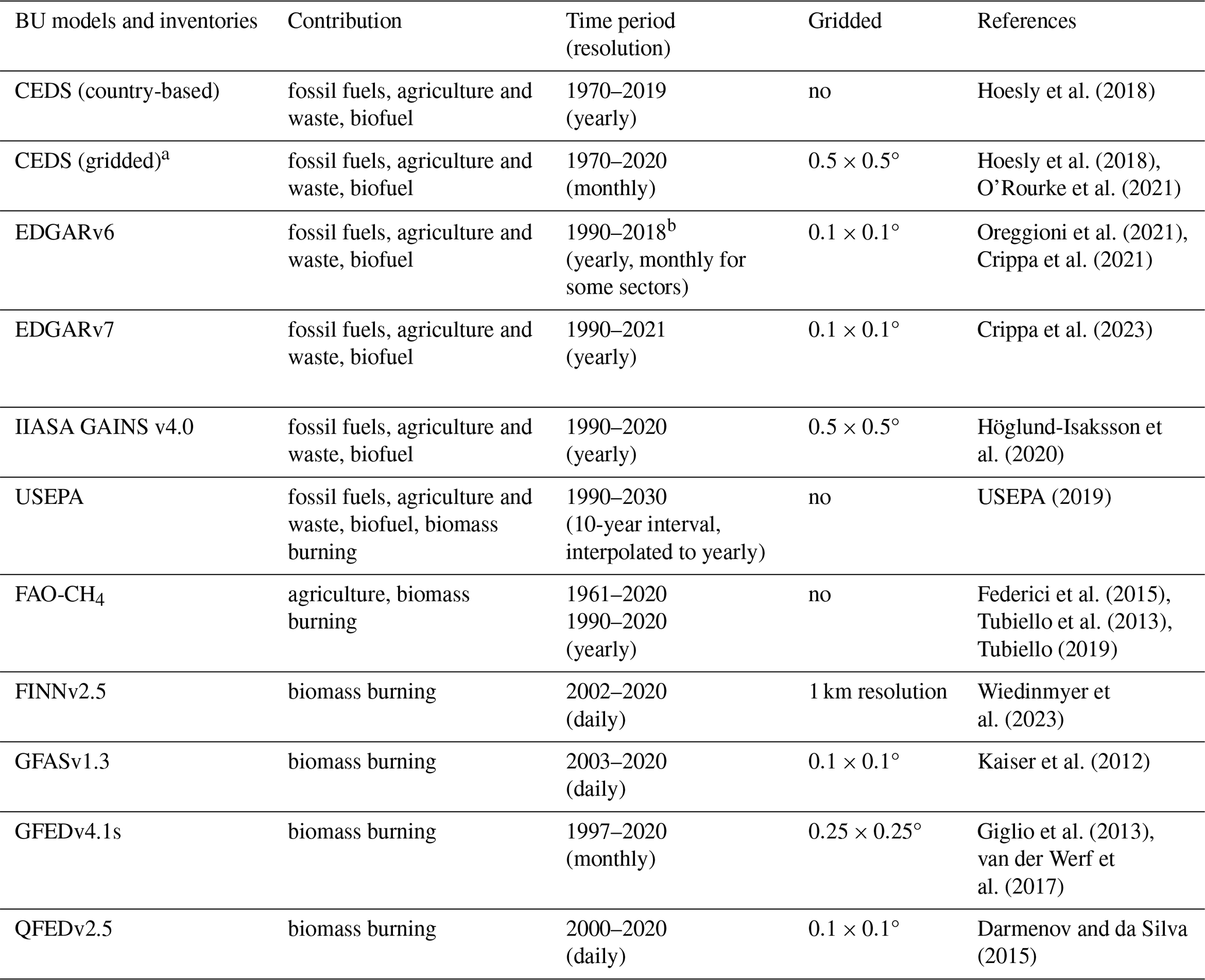
a Due to its limited sectoral breakdown, this data set is not used in Table 3. b Data set extends up to 2020, as stated in Sect. 2.2. and detailed in the Supplement (Sect. S4).
These inventory data sets report emissions from fossil fuel production, transmission, and distribution; livestock enteric fermentation; manure management and application; rice cultivation; and solid waste and wastewater. Since the level of detail provided by country and by sector varies among inventories, the data were reconciled into common categories according to Table S2. For example, agricultural waste-burning emissions treated as a separate category in EDGAR, GAINS, and FAO are included in the biofuel sector in the USEPA inventory and in the agricultural sector in CEDS. The GAINS, EDGAR, and FAO estimates of agricultural waste burning were excluded from this analysis (these amounted to 1–3 Tg CH4 yr−1 in recent decades) to prevent any potential overlap with separate estimates of biomass burning emissions (e.g. GFEDv4.1s; Giglio et al., 2013; van der Werf et al., 2017). In the inventories used here, emissions for a given region/country and a given sector are usually calculated following IPCC methodology (IPCC, 2006), as the product of an activity factor and its associated emission factor. An abatement coefficient may also be used, to account for any regulations implemented to control emissions (see e.g. Höglund-Isaksson et al., 2015). These data sets differ in their assumptions and data used for the calculation; however, they are not completely independent because they often use the same activity data, and some of them follow the same IPCC guidelines (IPCC, 2006). While the USEPA inventory adopts emissions reported by the countries to the UNFCCC, other inventories (FAOSTAT, EDGAR, and the GAINS model) produce their own estimates using a consistent approach for all countries, typically IPCC Tier 1 methods or deriving IPCC Tier 2 emission factors from country-specific information using a consistent methodology. These other inventories compile country-specific activity data and emission factor information or, if not available, adopt IPCC default factors (Tibrewal et al., 2024; Oreggioni et al., 2021; Höglund-Isaksson et al., 2020; Tubiello, 2019). CEDS takes a different approach (Hoesly et al., 2018) and combines data from GAINS, EDGAR, and FAO depending on the sector. Then their first estimates are scaled to match other individual or region-specific inventory values when available. This process maintains the spatial information in the default emission inventories while preserving consistency with country level data. The FAOSTAT data set (hereafter FAO-CH4) provides estimates at the country level and is limited to agriculture (CH4 emissions from enteric fermentation, manure management, rice cultivation, energy usage, burning of crop residues, and prescribed burning of savannahs) and land use (peatland fires and biomass burning). FAO-CH4 uses activity data mainly from the FAOSTAT crop and livestock production database, as reported by countries to FAO (Tubiello et al., 2013), and applies mostly the Tier 1 IPCC methodology for emissions factors (IPCC, 2006), which depend on geographic location and development status of the country. For manure, the country-scale temperature was obtained from the FAO global agro-ecological zone database (GAEZv3.0, 2012). Although country emissions are reported annually to the UNFCCC by Annex-I countries, and episodically by non-Annex-I countries, data gaps of those national inventories do not allow the inclusion of these estimates in this analysis.
In this budget, we use the following versions of these inventories that were available at the start and during the analysis (see Table 1):
-
EDGARv6 provides yearly gridded emissions by sector from 1970 to 2018 (Crippa et al., 2021; Oreggioni et al., 2021; EDGARv6 website https://edgar.jrc.ec.europa.eu/dataset_ghg60 (last access: 1 April 2025); Monforti Ferrario et al., 2021).
-
EDGARv7 provides yearly gridded emissions by sector from 1970 to 2020 (monthly for some sectors), but emissions from fossil fuel energy are not separated (oil–gas and coal are lumped together – see Table S2) (EDGARv7 website: https://edgar.jrc.ec.europa.eu/dataset_ghg70 (last access: 1 April 2025); Crippa et al., 2023).
-
GAINS model scenario version 4.0 (Höglund-Isaksson et al., 2020) provides an annual sectorial gridded product from 1990 to 2020 both by country and gridded. The USEPA (USEPA, 2019) provides 5-year sectorial totals by country from 1990 to 2020 (estimates from 2015 onward are a projection), with no gridded distribution available. The USEPA data set was linearly interpolated to provide yearly values from 1990–2020.
-
CEDS version v_2021_04_21 provides gridded monthly and annual country-based emissions by sector from 1970 to 2019 (Hoesly et al., 2018; O'Rourke et al., 2021). Fossil fuel emissions for 2020 have been updated using the methodology described for CO in Zheng et al. (2023).
-
FAO-CH4 (database accessed in December 2022, FAO, 2022) contains annual country level data for the period 1961–2020, for rice, manure, and enteric fermentation and for 1990–2020 for burning savannah, crop residue, and non-agricultural biomass burning.
3.1.2 Total direct anthropogenic emissions
We calculated separately the total anthropogenic emissions for each inventory by adding its values for “agriculture and waste”, “fossil fuels”, and “biofuels” with additional large-scale biomass burning emissions data (Sect. 3.1.5). This method avoids double counting and ensures consistency within each inventory. This approach was used for the EDGARv6 and v7, CEDS, and GAINS inventories, but we kept the USEPA inventory as originally reported because it includes its own estimates of biomass burning emissions. FAO-CH4 was only included in the range reported for the “agriculture and waste” category. For the latter, we calculated the range and mean value as the sum of the mean and range of the three anthropogenic subcategory estimates “enteric fermentation and manure”, “rice”, and “landfills and waste”. The values reported for the upper-level anthropogenic categories (“agriculture and waste”, “fossil fuels”, and “biomass burning and biofuels”) are therefore consistent with the sum of their subcategories, although there might be small percentage differences between the reported total anthropogenic emissions and the sum of the three upper-level categories. This approach provides a more accurate representation of the range of emission estimates, avoiding an artificial expansion of the uncertainty attributable to subtle differences in the definition of subsector categorisations between inventories.
Table 2Biogeochemical models that computed wetland emissions used in this study. Model runs were performed with two climate inputs: CRU and GSWP3-W5E5. Models were run with prognostic (using their own calculation of wetland areas) and/or diagnostic (using WAD2M (Zhang et al., 2021b)) wetland surface areas (see Sect. 3.2.1).
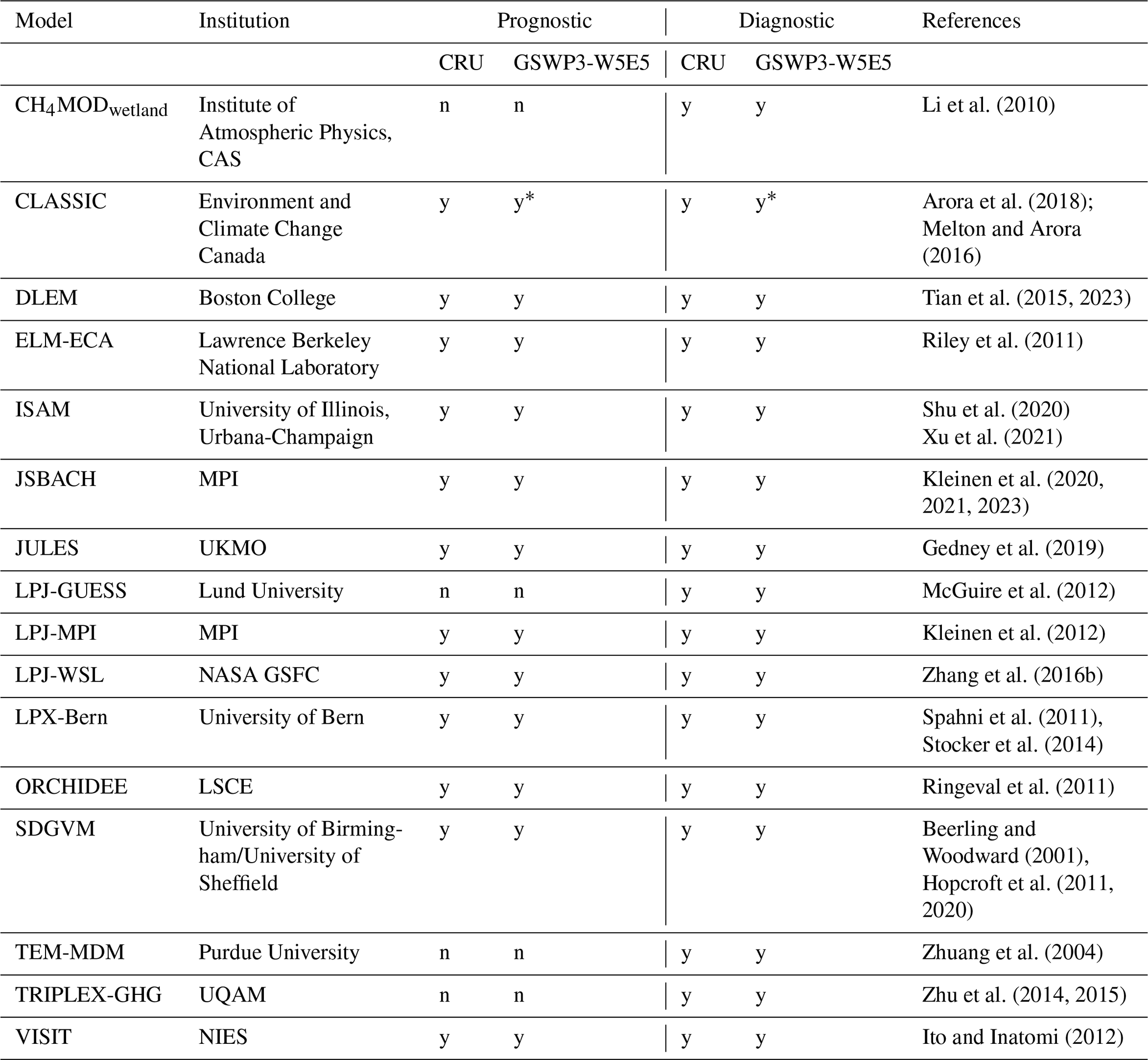
* CLASSIC uses GSWP3-W5E version 2 that covers the time period till 2016. All other models use GSWP-W5E5 version 3.
Table 3Global methane emissions by source type (in Tg CH4 yr−1) from Saunois et al. (2020) (left column pair) and from this work using bottom-up and top-down approaches. Because top-down models cannot fully separate individual processes, only five categories of emissions are provided (see text). Uncertainties are reported as [min–max] range of reported studies. The mean, minimum, and maximum values are calculated while discarding outliers, for each category of source and sink. As a result, discrepancies may occur when comparing the sum of categories and their corresponding total due to differences in outlier detections. Differences of 1 Tg CH4 yr−1 in the totals can also occur due to rounding errors. Compared to Saunois et al. (2020), emissions are split between “direct anthropogenic” emissions and “natural and indirect anthropogenic” sources. We also propose an estimate of the double counting between bottom-up wetland and inland freshwater ecosystem emissions. NA denotes “not available”.
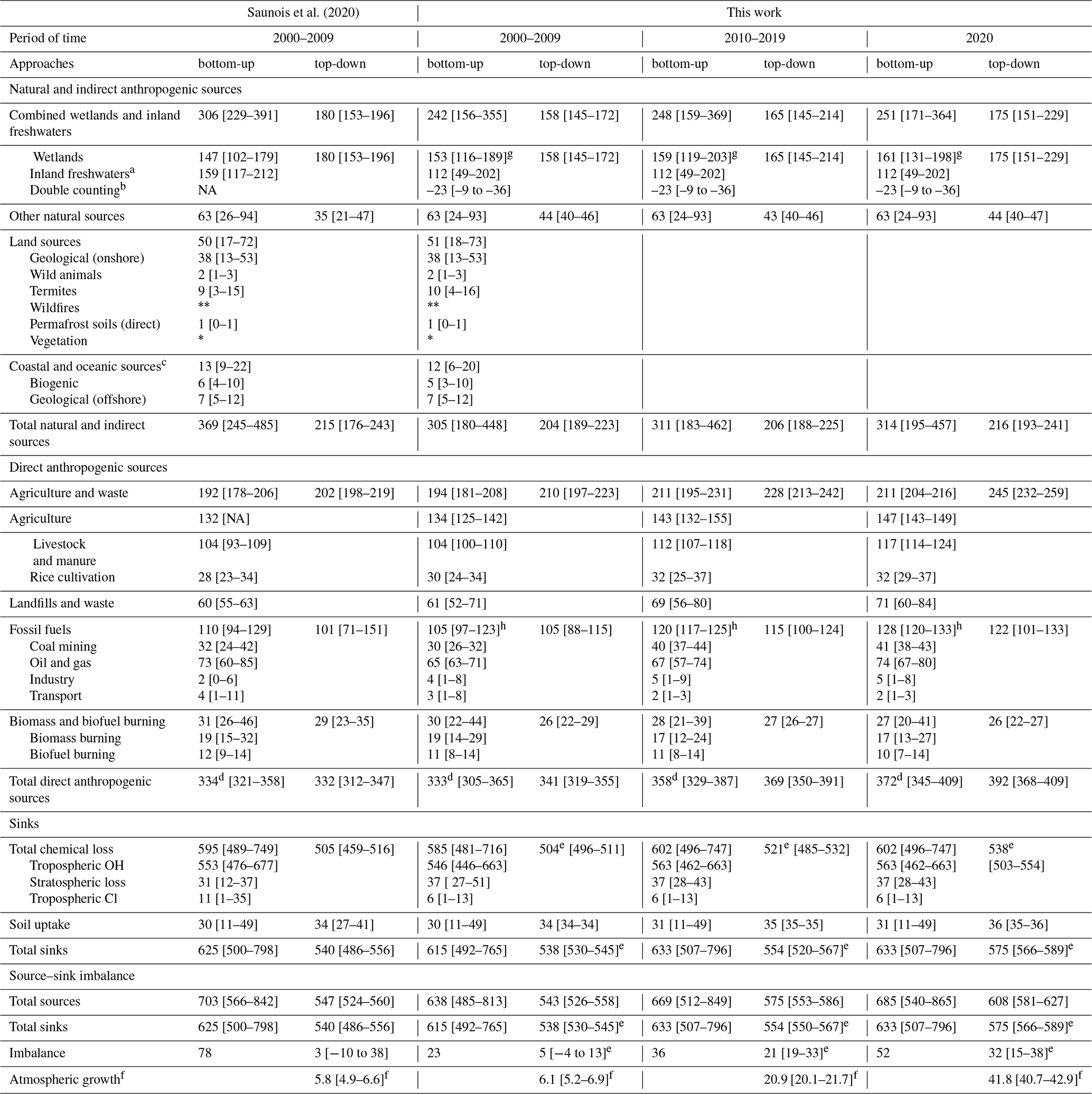
* Uncertain but likely small for upland forest and aerobic emissions, potentially large for forested wetland, but likely included elsewhere. We stop reporting this value to avoid potential double counting with satellite-based products of biomass burning (see Sect. 3.1.5). a Freshwater includes lakes, ponds, reservoirs, streams, and rivers; part of it is due to anthropogenic disturbances estimated in Sect. 3.2.2. b The double counting estimate is discussed in Sect. 3.2.2. c Flux from hydrates considered at 0 for this study is included, including estuaries. d Total anthropogenic emissions are based on estimates of full anthropogenic inventory and not on the sum of “agriculture and waste”, “fossil fuels“ and “biofuel and biomass burning” categories (see Sect. 3.1.2). e Some inversions did not provide the chemical sink. These values are derived from a subset of the inversion ensemble. f Atmospheric growth rates are given in the same unit (Tg CH4 yr−1), based on the conversion factor of 2.75 Tg CH4 ppb−1 given by Prather et al. (2012) and the atmospheric growth rates provided in the text (in ppb yr−1). g Here the numbers are from prognostic runs. To ensure a fair comparison with previous budgets (Saunois et al., 2020), the numbers are 163 [117–195] for 2000–2009 from diagnostic runs with CRU/CRU-JRA-55 climate inputs (see Sect. 3.2.1). h Up to 8 Tg of additional emissions could account for ultra-emitters (Lauvaux et al., 2022), as in Tibrewal et al. (2024), that are fully or partly missed in regular anthropogenic inventories.
Based on the ensemble of databases detailed above, total direct anthropogenic emissions were 358 [329–387] Tg CH4 yr−1 for the decade 2010–2019 (Table 3, including biomass and biofuel burning) and 331 [305–365] Tg CH4 yr−1 for the decade 2000–2009. Our estimate for the 2000–2009 decade is within the range of Saunois et al. (2020) (334 [321–358]), Saunois et al. (2016) (338 Tg CH4 yr−1 [329–342]), and Kirschke et al. (2013) (331 Tg CH4 yr−1 [304–368]) for the same period. The slightly larger range reported herein with respect to previous estimates is due to the USEPA lower estimate for agriculture, waste, and fossil emissions associated with the lowest estimate of biomass burning.
Figure 2 (left) summarises or projects global CH4 emissions of anthropogenic sources (including biomass and biofuel burning) by different data sets between 2000 and 2050. The data sets consistently estimate total anthropogenic emissions of ∼ 300 Tg CH4 yr−1 in 2000. For the Sixth Assessment Report of the IPCC, seven main Shared Socioeconomic Pathways (SSPs) were defined for future climate projections in the Coupled Model Intercomparison Project 6 (CMIP6) (Gidden et al., 2019; O'Neill et al., 2016) ranging from 1.9 to 8.5 W m−2 radiative forcing by the year 2100 (as shown by the number in the SSP names). For the 1970–2015 period, historical emissions used in CMIP6 (Feng et al., 2019) combine anthropogenic emissions from CEDS (Hoesly et al., 2018) and a climatological value from the GFEDv4.1s biomass burning inventory (van Marle et al., 2017). The harmonised scenarios used for CMIP6 activities start in 2015 at 388 Tg CH4 yr−1, which corresponds to the higher range of our estimates. Since CH4 emissions continue to track scenarios that assume no or minimal climate policies (SSP5 and SSP3), it may indicate that climate policies, when present, have not yet produced sufficient results to change the emissions trajectory substantially (Nisbet et al., 2019). After 2015, the SSPs span a range of possible outcomes, but current emissions appear likely to follow the higher-emission trajectories, given that over the past decade their trend has followed such trajectories and because the peak emission year has not yet been reached. High or medium emission reduction rates as suggested by scenarios SSP1 and SSP2 have not yet happened. This illustrates the challenge of methane mitigation that lies ahead to help reach the goals of the Paris Agreement (Nisbet et al., 2020; Shindell et al., 2024). In addition, estimates of methane atmospheric concentrations (Meinshausen et al., 2017, 2020) from the harmonised scenarios (Riahi et al., 2017) indicate that observations of global CH4 concentrations fall well within the range of scenarios in absolute values, but their trend over the past few years is closest to those of scenario SSP5-8.5 (Fig. 2 right). The CH4 concentrations are estimated using a simple exponential decay with inferred natural emissions (Meinshausen et al., 2011), and the emergence of any trend between observations and scenarios needs to be confirmed in the following years. However, the current observed concentrations and emissions estimates lie in the upper range of the former RCP scenarios starting in 2005 (Fig. S1). In the future, it will be important to monitor the trends from 2015 (the Paris Agreement) and from 2020 (Global Methane Pledge) estimated in inventories and from atmospheric observations and compare them to various scenarios.
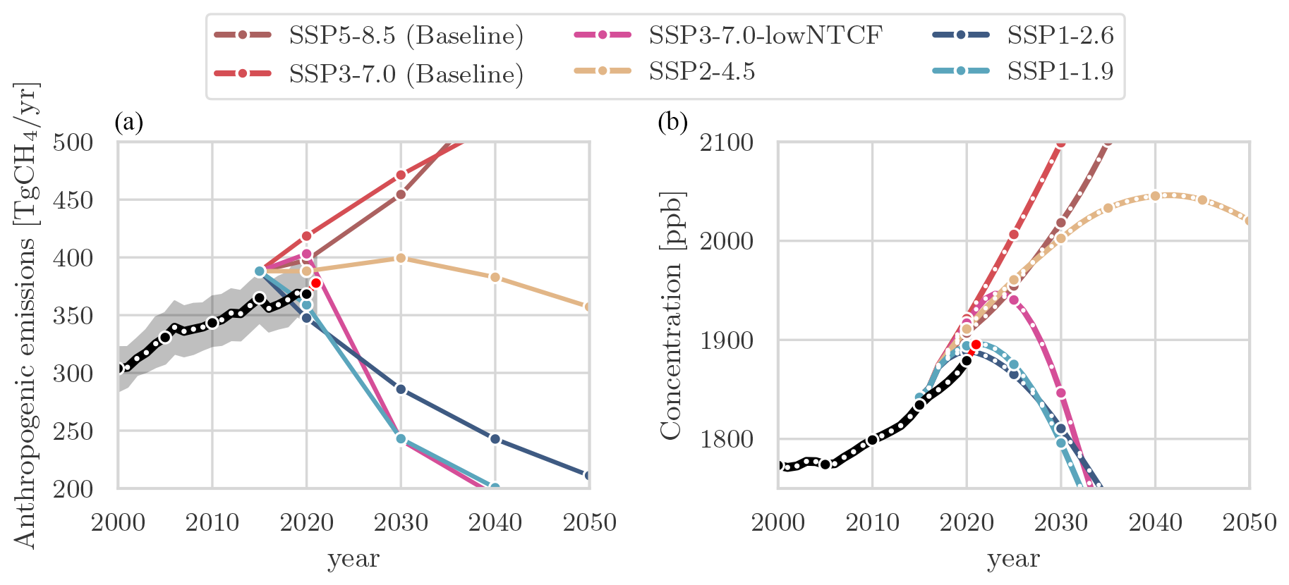
Figure 2(a) Global anthropogenic methane emissions (including biomass burning) over 2000–2050 from historical inventories (black line and shaded grey area) and future projections (coloured lines) (in Tg CH4 yr−1) from selected scenarios harmonised with historical emissions (CEDS) for CMIP6 activities (Gidden et al., 2019). Historical mean emissions correspond to the average of anthropogenic inventories listed in Table 1 added to the GFEDv4.1s (van der Werf et al., 2017) biomass burning historical emissions. (b) Global atmospheric methane concentrations for NOAA surface site observations (black) and projections based on SSPs (Riahi et al., 2017) with concentrations estimated using MAGICC (Meinshausen et al., 2017, 2020). Red dots show the last year available (2022 for observations).
3.1.3 Fossil fuel production and use
Most anthropogenic CH4 emissions related to fossil fuels come from the exploitation, transportation, and usage of coal, oil, and natural gas. Additional emissions reported in this category include small industrial contributions such as the production of chemicals and metals, fossil fuel fires (e.g. underground coal mine fires and the Kuwait oil and gas fires), and transport (road and non-road transport). CH4 emissions from the oil processing industry (e.g. refining) and production of charcoal are estimated to be a few teragrams of CH4 per year only and are included in the transformation industry sector in the inventory. Fossil fuel fires are included in the subcategory “oil and gas”. Emissions from industry, road transport, and non-road transport are reported apart from the two main subcategories “oil and gas” and “coal”, as in Saunois et al. (2020) and contrary to Saunois et al. (2016); each of these amounts to about 2 to 5 Tg CH4 yr−1 (Table 3). The large range (1–9 Tg CH4 yr−1) is attributable to difficulties in allocating some sectors to these subsectors consistently among the different inventories (see Table S2). The spatial distribution of CH4 emissions from fossil fuels is presented in Fig. 3 based on the mean gridded maps provided by CEDS, EDGARv6, and GAINS for the 2010–2019 decade; the USEPA lacks a gridded product.
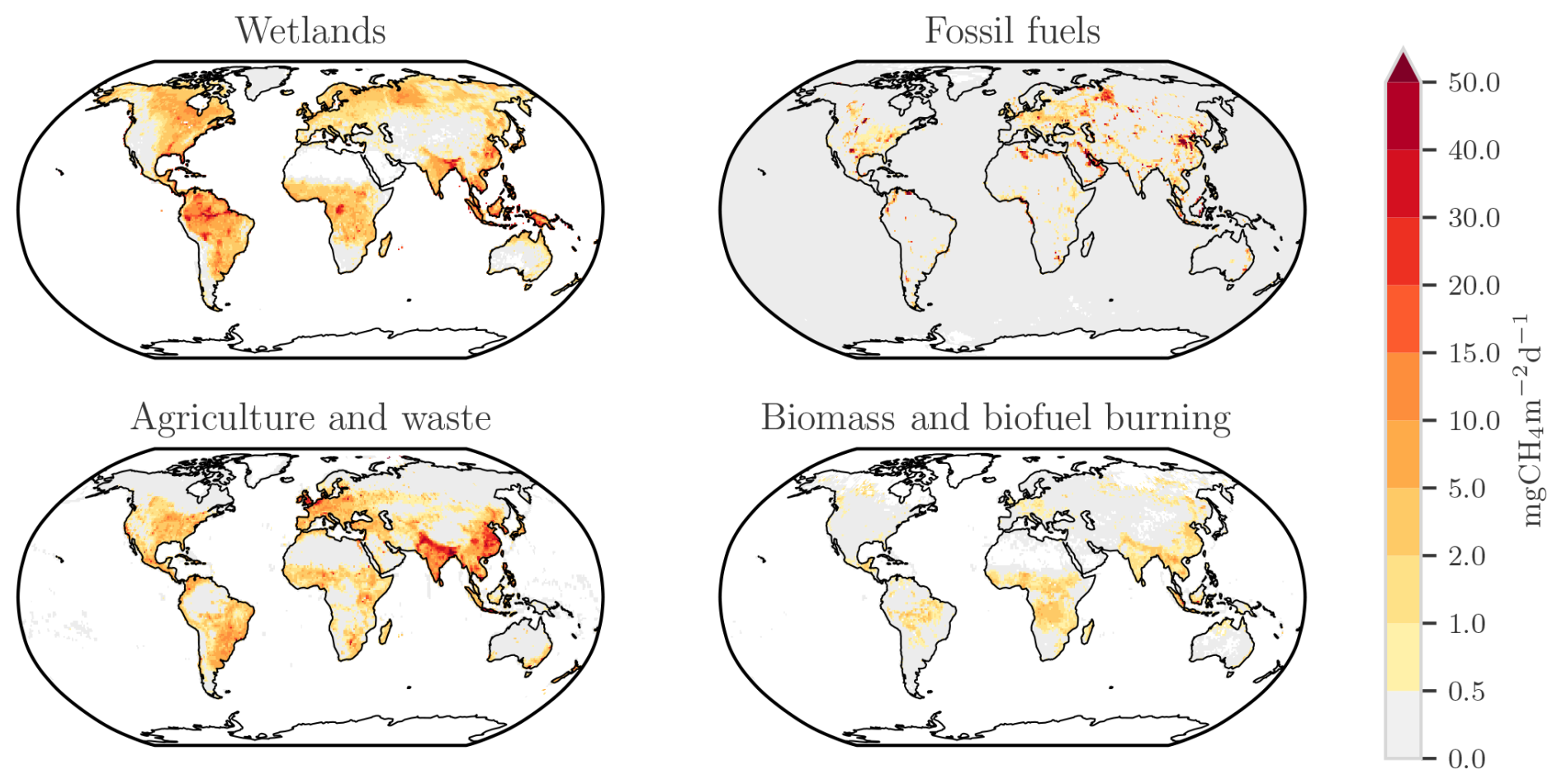
Figure 3Methane emissions from four source categories: natural wetlands (excluding lakes, ponds, and rivers), biomass and biofuel burning, agriculture and waste, and fossil fuels for the 2010–2019 decade (in mg CH4 m−2 d−1). The wetland emission map represents the mean daily emission average of the 16 biogeochemical models listed in Table 2 and over the 2010–2019 decade. Fossil fuel and agriculture and waste emission maps are derived from the mean estimates of gridded CEDS, EGDARv6, EDGARv7, and GAINS models. The biomass and biofuel burning map results from the mean of the biomass burning inventories listed in Table 1 added to the mean of the biofuel estimate from CEDS (O'Rourke et al., 2021), EDGARv6 (Crippa et al., 2021), EDGARv7 (Crippa et al., 2023), and GAINS (Höglund-Isaksson et al., 2020) models.
Global mean emissions from fossil-fuel-related activities, other industries, and transport are estimated from the four global inventories (Table 1) to be 120 [117–125] Tg CH4 yr−1 for the 2010–2019 decade (Table 3), but with large differences in the rate of change during this period across inventories. The sector accounts on average for 34 % (range 31 %–42 %) of total global anthropogenic emissions in 2010–2019. This contribution has slightly increased from 32 % on average in 2000–2009.
Coal mining
During mining, CH4 is emitted primarily from ventilation shafts, where large volumes of air are pumped in and out of the mine to keep the CH4 mixing ratio below 0.5 % to avoid accidental ignition and from dewatering operations. In countries of the Organization for Economic Co-operation and Development (OECD), coalbed CH4 is often extracted as fuel up to 10 years before the coal mine starts operation, thereby reducing the CH4 channelled through ventilation shafts during mining. In many countries, large quantities of ventilation air CH4 are still released to the atmosphere or flared, despite efforts to extend coal mine gas recovery under the UNFCCC Clean Development Mechanism (http://cdm.unfccc.int, last access: 1 April 2025). CH4 leaks also occur during post-mining handling, processing, and transportation. Some CH4 is released from coal waste piles and abandoned mines; while emissions from these sources were believed to be low (IPCC, 2000), recent work has estimated these at 22×109 m3 (compared to 103×109 m3 from functioning coal mines) in 2010 with emissions projected to increase into the future (Kholod et al., 2020).
In 2020, more than 35 % (IEA, 2023a) of the world's electricity is still produced from coal. This contribution grew in the 2000s at the rate of several percent per year, driven by Asian economic growth where large reserves exist, but global coal consumption declined between 2014 and 2020. In 2020, the top 10 largest coal-producing nations accounted for ∼ 90 % of total world CH4 emissions from coal mining; among them, the top three producers (China, the USA, and India) produced almost two-thirds (66 %) of the world's coal (IEA, 2021).
Global estimates of CH4 emissions from coal mining show a reduced range of 37–44 Tg CH4 yr−1 for 2010–2019 (Table 3), compared to the previous estimate for 2008–2017 in Saunois et al. (2020) reporting a range of 29–61 Tg CH4 yr−1 for 2008–2017. This reduced range probably results from using similar activity data (mostly from IEA statistics) in the different inventories. The highest value of the range in Saunois et al. (2020) came from the CEDS inventory, while the lowest came from the USEPA. CEDS seems to have revised downward their estimate compared to the previous version used in Saunois et al. (2020). There were previously large discrepancies in Chinese coal emissions, with a large overestimation from EDGARv4.2, on which CEDS was based. As highlighted by Liu et al. (2021a), a county-based inventory of Chinese methane emissions also confirms the overestimation of previous EDGAR inventories and estimated total anthropogenic Chinese emissions at 38.2 ± 5.5 Tg CH4 yr−1 for 2000–2008 (Liu et al., 2021a). Coal mining emission factors depend strongly on the type of coal extraction (underground mining emits up to 10 times more than surface mining), the geological underground structure (region-specific), history (basin uplift), and the quality of the coal (brown coal (lignite) emits less than hard coal (anthracite)). Finally, the different emission factors derived for coal mining are the main reason for the differences between inventories globally (Fig. 2).
For the 2010–2019 decade, methane emissions from coal mining represent 33 % of total fossil-fuel-related emissions of CH4 (40 [37–44] Tg CH4 yr−1; Table 3). An additional assumed very small source corresponds to fossil fuel fires, which are mostly underground coal fires. This source is estimated at around 0.15 Tg yr−1 in EDGARv7, though this value remains the same across EDGAR versions and for all years despite the changes in coal production, which could influence this estimate. However, to date, insufficient data are available to better estimate this largely unknown source.
Oil and natural gas systems
This subcategory includes emissions from both conventional and shale oil and gas exploitation. Natural gas is composed primarily of CH4, so both fugitive and planned emissions during the drilling of wells in gas fields, extraction, transportation, storage, gas distribution, end use, and incomplete combustion in gas flares emit CH4 (Lamb et al., 2015; Shorter et al., 1996). Persistent fugitive emissions (e.g. due to leaky valves and compressors) should be distinguished from intermittent emissions due to maintenance (e.g. purging and draining of pipes) or incidents. During transportation, fugitive emissions can occur in oil tankers, fuel trucks, and gas transmission pipelines, attributable to corrosion, manufacturing, and welding faults. According to Lelieveld et al. (2005), CH4 fugitive emissions from gas pipelines should be relatively low; however, old distribution networks in some cities may have higher rates, especially those with cast-iron and unprotected steel pipelines (Phillips et al., 2013). Measurement campaigns in cities within the USA (e.g. McKain et al., 2015) and Europe (e.g. Defratyka et al., 2021) revealed that significant emissions occur in specific locations (e.g. storage facilities, city natural gas fuelling stations, well and pipeline pressurisation/depressurisation points, sewage systems, and furnaces of buildings) along the distribution networks (e.g. Jackson et al., 2014; McKain et al., 2015; Wunch et al., 2016). However, CH4 emissions vary significantly from one city to another depending, in part, on the age of city infrastructure and the quality of its maintenance, making urban emissions difficult to scale up from measurement campaigns, although attempts have been made (e.g. Defratyka et al., 2021). In many facilities, such as gas and oil fields, refineries, and offshore platforms, most of the associated and other waste gas generated will be flared for security reasons with almost complete conversion to CO2; however, due to the large quantities of waste gas generated, small fractions of gas still being vented make up relatively large quantities of methane. These two processes are usually considered together in inventories of oil and gas industries. In addition, single-point failure of natural gas infrastructure can leak CH4 at high rate for months, such as at the Aliso Canyon blowout in Los Angeles, CA (Conley et al., 2016), or the shale gas well blowout in Ohio (Pandey et al., 2019), thus hampering emission control strategies. Production of natural gas from the exploitation of hitherto unproductive rock formations, especially shale, began in the 1970s in the USA on an experimental or small-scale basis, and then, from the early 2000s, exploitation started at a large commercial scale. The shale gas contribution to total dry natural gas production in the USA reached 82 % in 2023, growing rapidly from 48 % in 2013 (IEA, 2023b). The possibly larger emission factors from shale gas compared to conventional gas have been widely debated (e.g. Cathles et al., 2012; Howarth, 2019; Lewan, 2020). The latest studies tend to infer emission factors from the oil–gas production chain of about 1 % to 6 % (e.g. Schneising et al., 2020; Varon et al., 2023; Zhang et al., 2020), but the loss rate could be as high as more than 10 % in low-producing well sites (e.g. Omara et al., 2022, Williams et al., 2025).
CH4 emissions from oil and natural gas systems vary greatly in different global inventories (67 to 80 Tg yr−1 in 2020; Table 3). The inventories generally rely on the same sources and magnitudes for activity data, with the derived differences therefore resulting primarily from different methodologies and parameters used, including emission factors. Those factors are country- or even site-specific, and the few field measurements available often combine oil and gas activities (Brandt et al., 2014), resulting in high uncertainty in emission estimates for many major oil- and gas-producing countries. Depending on the region, the IPCC 2006 default emission factors may vary by 2 orders of magnitude for oil production and 1 order for gas production. For instance, the GAINSv4.0 estimate of CH4 emissions from US oil and gas systems in 2015 is 16 Tg, which is almost twice as high as EDGARv8.0 (EDGAR, 2023) at 8.4 Tg and the USEPA (USEPA, 2019) at 9.5 Tg. The difference can partly be explained by GAINS using a bottom-up methodology to derive country- and year-specific flows of associated petroleum gas and attributing these to recovery/reinjection, to flaring or venting (Höglund-Isaksson, 2017), and partly to GAINS using a higher emission factor for unconventional gas production (Höglund-Isaksson et al., 2020). Recent quantifications using satellite observations and inversion estimate a relatively stable trend for US oil and gas system emissions since 2010, with Lu et al. (2023) estimating 14.6 Tg for 2010, 15.9 Tg for 2014, and 15.6 Tg for 2019; Shen et al. (2022) estimating a mean of 12.6 Tg for 2018–2020; and Maasakkers et al. (2021) a mean of 11.1 Tg for 2010 to 2015. The stable top-down trend for the USA appears not well captured in the bottom-up inventories from GAINS and EDGAR, which tend to show an increasing trend driven by an increase in production volumes.
Most recent studies (e.g. Zhang et al., 2020; Shen et al., 2023; Li et al., 2024, Tibrewal et al., 2024; Sherwin et al., 2024) still suggest that the methane emissions from oil and gas industry are underestimated by inventories, industries, and agencies, including the USEPA and UNFCCC reporting. Lauvaux et al. (2022) showed that emissions from a few high-emitting facilities, i.e. super-emitters (> 20 t h−1), which are usually sporadic in nature and not accounted for in the inventories, could represent 8 %–12 % of global oil and gas emissions, or around 8 Tg CH4 yr−1. These high-emitting points, located on the conventional part of the facilities, could be avoided through better operating conditions and repair of malfunctions. Over the last decade, absolute CH4 emissions have almost certainly increased, since US crude oil production doubled and natural gas production rose by about 50 % (IEA, 2023a). However, global implications of the rapidly growing shale gas activity in the USA remain to be determined precisely.
For the 2010–2019 decade, CH4 emissions from upstream and downstream oil and natural gas sectors are estimated to represent about 56 % of total fossil CH4 emissions (67 [57–74] Tg CH4 yr−1; Table 3) based on global inventories, with a lower uncertainty range than for coal emissions for most countries. However, it is worth noting that 8 Tg CH4 yr−1 should be added on top of this estimate to acknowledge the ultra-emitter contribution, as done in Tibrewal et al. (2024).
3.1.4 Agriculture and waste sectors
This main category includes CH4 emissions related to livestock production (i.e. enteric fermentation in ruminant animals and manure management), rice cultivation, landfills, and wastewater handling. Of these activities, globally and in most countries, livestock is by far the largest source of CH4, followed by waste handling and rice cultivation. Conversely, field burning of agricultural residues is a minor source of CH4 reported in emission inventories (a few teragrams at the global scale). The spatial distribution of CH4 emissions from agriculture and waste handling is presented in Fig. 3 based on the mean gridded maps provided by CEDS, EDGARv6, and GAINS over the 2010–2019 decade.
Global emissions from agriculture and waste for the period 2010–2019 are estimated to be 211 [195–231] Tg CH4 yr−1 (Table 3), representing 60 % of total direct anthropogenic emissions. Agriculture emissions amount to 144 Tg CH4 yr−1, 40 % of the direct anthropogenic emissions, with the rest coming from the fossil fuel sector (34 %), waste (19 %), and biomass (5 %) and biofuel (3 %) burning.
Livestock: fermentation and manure management
Enteric domestic ruminants such as cattle, buffalo, sheep, goats, and camels emit CH4 as a by-product of the anaerobic microbial activity in their digestive systems (Johnson et al., 2002). The very stable temperatures (about 39 °C) and pH (6.5–6.8) within the rumen of domestic ruminants, along with a constant plant matter flow from grazing (cattle graze many hours per day), allow methanogenic Archaea residing within the rumen to produce CH4. CH4 is released from the rumen mainly through the mouth of multi-stomached ruminants (eructation, ∼ 90 % of emissions) or absorbed in the blood system. The CH4 produced in the intestines and partially transmitted through the rectum is only ∼ 10 % (Hill et al., 2016).
The total number of livestock continues to grow steadily. There are currently (2020) about 1.5 billion cattle globally, almost 1.3 billion sheep, and nearly as many goats (http://www.fao.org/faostat/en/#data/GE, last access: 1 April 2025). Livestock numbers are linearly related to CH4 emissions in inventories using the Tier 1 IPCC approach such as FAOSTAT. In practice, some non-linearity may arise due to dependencies of emissions on the total weight of the animals and their diet, which are better captured by Tier 2 and higher approaches. Cattle, due to their large population, large individual size, and particular digestive characteristics, account for the majority of enteric fermentation CH4 emissions from livestock worldwide (Tubiello, 2019; FAO, 2022), particularly in intensive agricultural systems in wealthier and emerging economies, including the USA (USEPA, 2016). CH4 emissions from enteric fermentation also vary from one country to another as cattle may experience diverse living conditions that vary spatially and temporally, especially in the tropics (Chang et al., 2019).
Anaerobic conditions often characterise manure decomposition in a variety of manure management systems globally (e.g. liquid/slurry treated in lagoons, ponds, tanks, or pits), with the volatile solids in manure producing CH4. In contrast, when manure is handled as a solid (e.g. in stacks or dry lots) or deposited on pasture, range, or paddock lands, it tends to decompose aerobically and to produce little or no CH4. However aerobic decomposition of manure tends to produce nitrous oxide (N2O), which has a larger global warming impact than CH4. Ambient temperature, moisture, energy contents of the feed, manure composition, and manure storage or residency time affect the amount of CH4 produced. Despite these complexities, most global data sets used herein apply a simplified IPCC Tier 1 approach, where amounts of manure treated depend on animal numbers and simplified climatic conditions by country.
Global CH4 emissions from enteric fermentation and manure management are estimated in the range of 114–124 Tg CH4 yr−1, for the year 2020, in the GAINS model and CEDS, USEPA, FAO-CH4, and EDGARv7 inventories (Table 3). Using the Tier 2 method adopted from the 2019 refinement to 2006 IPCC guidelines, a recent study (Zhang et al., 2022) estimated that global CH4 emissions from livestock increased from 31.8 [26.5–37.1] (mean [minimum−maximum] of 95 % confidence interval) Tg CH4 yr−1 in 1890 to 131.7 [109.6–153.7] Tg CH4 yr−1 in 2019, a 4-fold increase in the past 130 years. Chang et al. (2021) estimate enteric fermentation and manure management emissions based on mixed Tier 1–2 and Tier 1 approaches and calculate livestock emissions of 120 ± 13 and 136 ± 15 Tg CH4 yr−1 respectively for 2018. Chang et al. (2021) and Zhang et al. (2022) estimates for 2018 and 2019 are on average a bit higher than the inventories estimates but in agreement considering the uncertainties. It is worth recalling here that the ranges provided in this study correspond to the minimum–maximum of the existing estimates and do not include the uncertainty of the individual estimate; these uncertainties could be larger than the range proposed here.
For the period 2010–2019, we estimated total emissions of 112 [107–118] Tg CH4 yr−1 for enteric fermentation and manure management, about one-third of total global anthropogenic emissions (Table 3).
Rice cultivation
Most of the world's rice is grown in flooded paddy fields (Elphick, 2010). The water management systems, particularly flooding, used to cultivate rice are one of the most important factors influencing CH4 emissions and one of the most promising approaches for CH4 emission mitigation: periodic drainage and aeration not only cause existing soil CH4 to oxidise, but also inhibit further CH4 production in soils (Simpson et al., 1995; USEPA, 2016; Zhang et al., 2016a). Upland rice fields are not typically flooded and therefore are not a significant source of CH4. Other factors that influence CH4 emissions from flooded rice fields include fertilisation practices (i.e. the use of urea and organic fertilisers), soil temperature, soil type (texture and aggregated size), and rice variety and cultivation practices (e.g. tillage, seeding, and weeding practices) (Conrad et al., 2000; Kai et al., 2011; USEPA, 2012; Yan et al., 2009). For instance, CH4 emissions from rice paddies increase with organic amendments (Cai et al., 1997) but can be mitigated by applying other types of fertilisers (mineral, composts, biogas residues) or using wet seeding (Wassmann et al., 2000).
The geographical distribution of rice emissions has been assessed by global (e.g. Janssens-Maenhout et al., 2019; Tubiello, 2019; USEPA, 2012) and regional (e.g. Castelán-Ortega et al., 2014; Chen et al., 2013; Chen and Prinn, 2006; Peng et al., 2016; Yan et al., 2009; Zhang and Chen, 2014) inventories and land surface models (Li et al., 2005; Pathak et al., 2005; Ren et al., 2011; Spahni et al., 2011; Tian et al., 2010, 2011; Zhang et al., 2016a). The emissions show a seasonal cycle, peaking in the summer months in the extratropics, associated with monsoons and land management. Emissions from rice paddies are influenced not only by the extent of rice field area, but also by changes in the productivity of plants (Jiang et al., 2017) as these alter the CH4 emission factor used in inventories. However, the inventories considered herein are largely based on IPCC Tier 1 methods, which mainly scale with cultivated areas and include region-specific emission factors but do not account for changes in plant productivity and detailed cultivation practices.
The largest emissions from rice cultivation are found in Asia, accounting for 30 % to 50 % of global emissions (Fig. 3). The decrease in CH4 emissions from rice cultivation over recent decades is confirmed in most inventories because of the decrease in rice cultivation area, changes in agricultural practices, and a northward shift of rice cultivation since the 1970s, as in China (e.g. Chen et al., 2013).
Based on the global inventories considered in this study, global CH4 emissions from rice paddies are estimated to be 32 [25–37] Tg CH4 yr−1 for the 2010–2019 decade (Table 3), or about 9 % of total global anthropogenic emissions of CH4. These estimates are consistent with the 29 Tg CH4 yr−1 estimated for the year 2000 by Carlson et al. (2017).
Waste management
This sector includes emissions from managed and non-managed landfills (solid waste disposal on land) and wastewater handling, where all kinds of waste are deposited. CH4 production from waste depends on the pH, moisture, and temperature of the material. The optimum pH for CH4 emission is between 6.8 and 7.4 (Thorneloe et al., 2000). The development of carboxylic acids leads to low pH, which limits methane emissions. Food or organic waste, such as leaves and grass clippings, ferment quite easily, while wood and wood products generally ferment slowly and cellulose and lignin even more slowly (USEPA, 2010a).
Waste management was responsible for about 11 % of total global direct anthropogenic CH4 emissions in 2000 (Kirschke et al., 2013). A recent assessment of CH4 emissions in the USA found landfills to account for almost 26 % of total US anthropogenic CH4 emissions in 2014, the largest contribution of any single CH4 source in the USA (USEPA, 2016). In Europe, gas control has been mandatory on all landfills since 2009, and more importantly for CH4 emissions, the EU Landfill Directive (1999) with subsequent amendments, has diverted most biodegradable waste away from landfills towards source separation, recycling, composting, and energy recovery, with a legally binding target not to landfill more than 10 % of municipal solid waste by 2035.
Wastewater from domestic and industrial sources is treated in municipal sewage treatment facilities and private effluent treatment plants. The principal factor in determining the CH4 generation potential of wastewater is the amount of degradable organic material in the wastewater. Wastewater with high organic content is treated anaerobically, which leads to increased emissions (André et al., 2014). Excessive and rapid urban development worldwide, especially in Asia and Africa, could enhance methane emissions from waste unless adequate mitigation policies are designed and implemented rapidly.
The GAINS model and CEDS and EDGAR inventories give robust emission estimates from solid waste in the range of 37–42 Tg CH4 yr−1 for the year 2019 and more uncertain wastewater emissions in the range 20–45 Tg CH4 yr−11.
In our study, the global emission of CH4 from waste management is estimated in the range of 56–80 Tg CH4 yr−1 for the 2010–2019 period with a mean value of 69 Tg CH4 yr−1, about 19 % of total global anthropogenic emissions (Table 3).
3.1.5 Biomass and biofuel burning
This category includes CH4 emissions from biomass burning in forests, savannahs, grasslands, peats, and agricultural residues, as well as from the burning of biofuels in the residential sector (stoves, boilers, fireplaces). Biomass and biofuel burning emit CH4 under incomplete combustion conditions (i.e. when oxygen availability is insufficient for complete combustion), for example in charcoal manufacturing and smouldering fires. The amount of CH4 emitted during the burning of biomass depends primarily on the amount of biomass, burning conditions, fuel moisture, and the specific material burned.
In this study, we use large-scale biomass burning (forest, savannah, grassland, and peat fires) from five biomass burning inventories (described below) and the biofuel burning contribution from anthropogenic emission inventories (EDGARv6 and v7, CEDS, GAINS, and USEPA). The spatial distribution of emissions from the burning of biomass and biofuel over the 2010–2019 decade is presented in Fig. 3 based on data listed in Table 1.
At the global scale, during the period of 2010–2019, biomass and biofuel burning generated CH4 emissions of 28 [21–39] Tg CH4 yr−1 (Table 3), of which 30 %–50 % is from biofuel burning.
Biomass burning
Fire is an important disturbance event in terrestrial ecosystems globally (van der Werf et al., 2010) and can be of either natural (typically ∼ 10 % of fires, ignited by lightning strikes or started accidentally) or anthropogenic origin (∼ 90 %, human-initiated fires) (USEPA, 2010b, Chap. 9.1). As previously noted all fires are counted as anthropogenic in Table 3. Anthropogenic fires are concentrated in the tropics and subtropics, where forests, savannahs, and grasslands may be burned to clear land for agricultural purposes or to maintain pastures and rangelands. Small fires associated with agricultural activity, such as field burning and agricultural waste burning, are often not detected by moderate-resolution remote sensing methods and are instead estimated based on cultivated area or through in situ measurements such as dedicated airborne campaigns (e.g. Barker et al., 2020).
Emission rates of biomass burning vary with biomass loading (depending on the biomes) at the location of the fire, the efficiency of the fire (depending on the vegetation type), the fire type (smouldering or flaming), and emission factor (mass of the considered species/mass of biomass burned). Depending on the approach, these parameters can be derived using satellite data and/or biogeochemical model or through simpler IPCC default approaches.
In this study, we use five products to estimate biomass burning emissions. The Global Fire Emission Database (GFED) is the most widely used global biomass burning emission data set and provides estimates from 1997 onwards. Here, we use GFEDv4.1s (van der Werf et al., 2017), based on the Carnegie–Ames–Stanford approach (CASA) biogeochemical model (van der Werf et al., 2010) driven by satellite-derived vegetation characteristics and burned area mostly from the MODerate resolution Imaging Sensor, MODIS (Giglio et al., 2013). GFEDv4.1s (with small fires) is available at a 0.25° resolution and on a daily basis from 1997 to 2020. One characteristic of the GFEDv4.1s burned area is that small fires are better accounted for compared to GFEDv4.1 (Randerson et al., 2012), increasing carbon emissions by approximately 35 % at the global scale. The latest version GFEDv5 (Chen et al., 2023) suggests a 61 % higher burned area than GFEDv4.1s, in closer agreement with burned area products from higher-resolution satellite sensors. The next budget would benefit from GFEDv5 to revisit the estimates of biomass burning emissions (which would likely go up) based on more specific comparison studies. The Quick Fire Emissions Dataset (QFED) is calculated using the fire radiative power (FRP) approach, in which the thermal energy emitted by active fires (detected by MODIS) is converted to an estimate of CH4 flux using biome-specific emissions factors and a unique method of accounting for cloud cover. Further information related to this method and the derivation of the biome-specific emission factors can be found in Darmenov and da Silva (2015). Here we use the historical QFEDv2.5 product available daily on a 0.1×0.1 grid for 2000 to 2020.
The Fire INventory from the National Center for Atmospheric Research (FINNv2.5; Wiedinmyer et al., 2023) provides daily, 1 km resolution estimates of gas and particle emissions from open burning of biomass (including wildfire, agricultural fires, and prescribed burning) over the globe for the period 2002–2020. FINNv2.5 uses MODIS and VIIRS satellite observations for active fires, land cover, and vegetation density.
We use v1.3 of the Global Fire Assimilation System (GFAS; Kaiser et al., 2012), which calculates emissions of biomass burning by assimilating fire radiative power (FRP) observations from MODIS at a daily frequency and 0.5° resolution and is available for 2000–2020.
The FAO-CH4 yearly biomass burning emissions are based on the most recent MODIS 6 burned area products (Prosperi et al., 2020), coupled with a pixel level (500 m) implementation of the IPCC Tier 1 approach, and are available from 1990 to 2020 (Table 1).
The differences in emission estimates for biomass burning arise from specific geographical and meteorological conditions and fuel composition, which strongly impact combustion completeness and emission factors. The latter vary greatly according to fire type, ranging from 2.2 g CH4 kg−1 dry matter burned for savannah and grassland fires up to 21 g CH4 kg−1 dry matter burned for peat fires (van der Werf et al., 2010). Biomass burning emissions encountered large interannual variability related to meteorological conditions, with generally higher emissions during El Niño periods as in 2019 (20 [14–28] Tg CH4 yr−1), 2015 (22 [15–28] Tg CH4 yr−1), and 2010 to a lesser extent (18 [15–29] Tg CH4 yr−1).
In this study, based on the five aforementioned products, biomass burning emissions are estimated at 17 Tg CH4 yr−1 [12–24] for 2010–2019, representing about 5 % of total global anthropogenic CH4 emissions (Table 3).
Biofuel burning
Burning of biomass to produce energy for domestic, industrial, commercial, or transportation purposes is hereafter called biofuel burning. A largely dominant fraction of CH4 emissions from biofuel burning comes from domestic cooking or heating in stoves, boilers, and fireplaces, mostly in open cooking fires where wood, charcoal, agricultural residues, or animal dung are burned. It is estimated that more than 2 billion people, mostly in developing countries, use solid biofuels to cook and heat their homes daily (André et al., 2014), yet CH4 emissions from biofuel combustion have received relatively little attention. Biofuel burning estimates are gathered from the CEDS, USEPA, GAINS, and EDGAR inventories. Due to the sectoral breakdown of the EDGAR and CEDS inventories, the biofuel component of the budget has been estimated as equivalent to the “RCO – Energy for buildings” sector as defined in Worden et al. (2017) and Hoesly et al. (2018) (Table S2). This is equivalent to the sum of the IPCC 1.A.4.a - Commercial/Institutional, 1.A.4.b - Residential, 1.A.4.c - Agriculture/Forestry/Fishing/Fish farms, and 1.A.5 - Non-Specified reporting categories. This definition is consistent with that used in Saunois et al. (2016) and Kirschke et al. (2013). While this sector incorporates biofuel use, it also includes the use of other combustible materials (e.g. coal or gas) for small-scale heat and electricity generation within residential and commercial premises. Data provided by the GAINS inventory suggest that this approach may overestimate biofuel emissions by between 5 % and 50 %. Further study into this category would be needed to better disentangle biofuels from fossil combustibles.
In our study, biofuel burning is estimated to contribute 11 [8–14] Tg CH4 yr−1 to the global CH4 budget, about 3 % of total global anthropogenic CH4 emissions for 2010–2019 (Table 3).
3.1.6 Other anthropogenic sources (not explicitly included in this study)
Other anthropogenic sources not included in this study are related to agriculture and land use management. In particular, increases in agricultural areas (such as global palm oil production) have led to the clearing of natural peat forests, reducing natural peatland area and associated natural CH4 emissions. Peatlands planted to forests (like in northern Europe) also lead to reduced CH4 emissions. While studies have long suggested that CH4 emissions from peatland drainage ditches are likely to be significant (e.g. Minkkinen and Laine, 2006; Peacock et al., 2021), CH4 emissions related to palm oil plantations have yet to be properly quantified (e.g. Manning et al., 2019). Taylor et al. (2014) have quantified global palm oil wastewater treatment fluxes to be 4 ± 32 Tg CH4 yr−1 for 2010–2013. This currently represents a small and highly uncertain source of methane but one potentially growing in the future.
3.2 Natural and indirect anthropogenic sources
As introduced in Sect. 2.4, natural and indirect anthropogenic sources refer to pre-agricultural CH4 emissions even if they are perturbed by anthropogenic climate change or other global change factors (e.g. eutrophication) and indirect emissions resulting from anthropogenic perturbation of the landscape (reservoirs) and the biogeochemical characteristics of soil. They include vegetated wetland emissions and inland freshwater systems (lakes, small ponds, reservoirs, and rivers), land geological sources (gas–oil seeps, mud volcanoes, microseepage, geothermal manifestations, and volcanoes), wild animals, wildfires, termites, thawing terrestrial and marine permafrost, and coastal and oceanic sources (biogenic, geological, and hydrate). In water-saturated or flooded ecosystems, the decomposition of organic matter gradually depletes most of the oxygen in the soil or the sediment zone, resulting in anaerobic conditions and CH4 production. Once produced, CH4 can reach the atmosphere through a combination of three processes: (1) diffusive loss of dissolved CH4 across the air–water boundary, (2) ebullition flux from sediments, and (3) flux mediated by emergent aquatic macrophytes and terrestrial plants (plant transport). On its way to the atmosphere, in the soil or water columns, CH4 can be partly or completely oxidised by microorganisms, which use CH4 as a source of energy and carbon (USEPA, 2010b). Concurrently, methane from the atmosphere can diffuse into the soil column and be oxidised (see Sect. 3.3.4 on soil uptake).
3.2.1 Wetlands
Wetlands are generally defined as ecosystems in which mineral or peat soils are water-saturated at some depth or where surface inundation (permanent or not) has a dominating influence on the soil biogeochemistry and determines the ecosystem species composition (USEPA, 2010b). To refine such an overly broad definition for CH4 emissions, we define wetlands as ecosystems with inundated or saturated soils or peats where anaerobic conditions below the water table lead to CH4 production (Matthews and Fung, 1987; USEPA, 2010b). Brackish water emissions are discussed separately in Sect. 3.2.6. Our definition of wetlands includes ombrotrophic and minerotrophic peatlands (i.e. bogs and fens), mineral soil wetlands (swamps and marshes), and seasonal or permanent floodplains. It excludes exposed water surfaces without emergent macrophytes, such as lakes, rivers, estuaries, ponds, and reservoirs (addressed in the next section), as well as rice agriculture (see Sect. 3.1.4, rice cultivation paragraph) and wastewater ponds. It also excludes coastal vegetated ecosystems (mangroves, seagrasses, salt marshes) with salinities usually > 0.5 (see Sect. 3.2.6). Even with this definition, some wetlands could be considered anthropogenic systems, being affected by human land use changes such as impoundment, drainage, or restoration (Woodward et al., 2012). In the following, we retain the generic denomination “wetlands” for natural and human-influenced wetlands, as discussed in Sect. 2.2.
The three most important factors influencing CH4 production in wetlands are the spatial and temporal extent of anoxia (linked to water saturation), temperature, and substrate availability (Valentine et al., 1994; Wania et al., 2010; Whalen, 2005; Delwiche et al., 2021; Knox et al., 2021).
Land surface models estimate CH4 emissions through a series of processes, including CH4 production, oxidation, and transport. The models are then forced with inputs accounting for changing environmental factors (Melton et al., 2013; Poulter et al., 2017; Tian et al., 2010; Wania et al., 2013; Xu et al., 2010). CH4 emissions from wetlands are computed as the product of an emission flux density and a CH4-producing area or surface extent (Bohn et al., 2015; Melton et al., 2013). The areal extent of different wetland types (having large differences in areal CH4 emission rates) appears to be a primary contributor to uncertainties in the absolute flux of CH4 emissions from wetlands, with meteorological response being the main source of uncertainty for seasonal and interannual variability (Poulter et al., 2017; Kuhn et al., 2021; Parker et al., 2022; McNicol et al., 2023; Karlson and Bastviken, 2023). However, large uncertainty remains in both spatial and temporal emission distributions, especially over tropical wetlands where data are lacking to evaluate the models but are nevertheless a key region for climate feedbacks (Nisbet, 2023; Zhang et al., 2023). Direct measurement campaigns and remote sensing are providing key insights into where to improve the land surface models (e.g. France et al., 2022; Shaw et al., 2022).
In this work, 16 land surface models computing net CH4 emissions (Table 2) were run under a common protocol with a spin-up using repeated climate data from 1901–1920 to pre-industrial conditions followed by a transient simulation through the end of 2020. Of the 16 models, 13 previously contributed to Saunois et al. (2020), and 3 models were new to this release (CH4MODwetland (Li et al., 2010), ISAM (Shu et al., 2020; Xu et al., 2021), and SDGVM (Beerling and Woodward, 2001; Hopcroft et al., 2011; Hopcroft et al., 2020)) (Table 2; see also in the Supplement Table S3 for a history of the contributing models). Climatic forcing uncertainties are considered in the ensemble estimate by using two climate data sets: CRU/CRU-JRA55 (Harris et al., 2014) and GSWP3-W5E5 (Dirmeyer et al., 2006; Kim, 2017; Lange, 2019; Cucchi et al., 2020). Atmospheric CO2 was also prescribed in the models. For all models, two wetland area dynamic schemes were applied: a diagnostic scheme using a remote-sensing-based wetland area and dynamics data set called WAD2M (Wetland Area Dynamics for Methane Modeling; Zhang et al., 2021a, b) available at 0.25° of horizontal resolution, as in Saunois et al. (2020), and a prognostic scheme using internal model-specific hydrologic models.
The diagnostic wetland extent product WAD2Mv1.0 (Zhang et al., 2021a) has been updated since the work of Saunois et al. (2020) to WAD2Mv2.0 (Zhang et al., 2021b) and extended to 2020. It uses the same Surface Water Microwave Product Series (SWAMPSv3.2) for capturing inundation dynamics (Jensen and McDonald, 2019), which was extended to 2020. To reduce potential double counting with the freshwater budget, the surface areas of rivers/streams and lakes/ponds are excluded by using the products Global River Widths from Landsat (GRWL) database v01.01 (Allen and Pavelsky, 2018) and HydroLAKES v1.0 (Messenger et al., 2006), instead of the Global Surface Water (GSW) product (Pekel et al., 2016) used in WAD2Mv1.0. The GRWL and HydroLAKES are also the data sets used separately in the upscaling of the freshwater budget, allowing for a more consistent approach between the wetland and freshwater CH4 budgets (Sect. 3.2.2). This update in WAD2M leads to a downward revised annual average wetland extent by 0.5 Mkm2 for the mid-high latitudes (mainly due to larger lake extent in HydroLAKES than in the GSW data set) with small impacts in other regions. However, since HydroLAKES includes only vectorised lakes larger than 0.1 km2, smaller lakes/ponds under 0.1 km2 are implicitly still included as wetlands in WAD2Mv2.0. For the high-latitude region, the recent peatland extent product from Hugelius et al. (2020) is applied, which indicates a slightly higher peatland area by 0.2 Mkm2, primarily in regions above 60° N, compared to the Northern Circumpolar Soil Carbon Database (NCSCD) product (Hugelius et al., 2013) used in WAD2Mv1.0. Rice agriculture was removed using the Monthly Irrigated and Rainfed Crop Areas (MIRCA2000; Portmann et al., 2010) data set from circa 2000, as a fixed distribution.
The combined remote-sensing and inventory WAD2Mv2.0 product leads to a maximum wetland area of 13.6 Mkm2 during the peak season (7.9 Mkm2 on annual average, with a range of 7.5 to 8.4 Mkm2 from 2000–2020, about 5.2 % of the global land surface). The largest wetland areas in WAD2Mv2.0 are in Amazonia, the Congo Basin, and the Western Siberian lowlands, which in previous studies were underestimated by inventories (Bohn et al., 2015). However, the SWAMPS v3.2 data set, which serves as a proxy of temporal variations in wetland extent, has had discontinuity issues over a few tropical hotspots since 2015 and hence affects the temporal variations in WAD2M. Consequently, this affects CH4 emissions estimates for a subset of land surface models that are particularly sensitive to inundation in these hotspots. Meanwhile, prognostic estimates show moderate consistency in capturing the spatial distribution of wetland areas with WAD2M, with an annual average wetland area of 8.0 ± 2.0 Mkm2 during the peak season for 2000–2020. The ensemble mean of annual wetland area anomaly by the prognostic models shows reasonable agreement with satellite-based estimates in capturing the response of wetland area to climate variations (Zhang et al., 2025), with higher agreement over temperate and boreal regions than in the tropics.
For the wetland methane emissions estimate, we use the decadal mean from the prognostic runs and adjust these flux estimates for double counting from inland waters (described in next section) given the reliance of the prognostic models on satellite flooded area data like WAD2Mv2 to parameterise maximum wetland extent (Zhang et al., 2025). The average emission from wetlands for 2010–2019 for the 16 models is plotted in Fig. 3. The zones with the largest emissions are the Amazon basin, equatorial Africa and Asia, Canada, western Siberia, eastern India, and Bangladesh. Regions where CH4 emissions have high intermodel agreement (defined as regions where mean flux is larger than the standard deviation of the models, on a decadal mean) represent 72 % of the total CH4 flux due to natural wetlands. The different sensitivities of the models to temperature, vapour pressure, precipitation, and radiation can generate substantially different patterns, such as in India. Emission estimates over regions with lower emissions (in total) are also consistently inferred between models (e.g. Scandinavia, continental Europe, eastern Siberia, central USA, and southern Africa).
The resulting global flux range for vegetated wetland emissions from the prognostic runs is 117–195 Tg CH4 yr−1 for the 2000–2020 period, with an average of 157 Tg CH4 yr−1 and a 1σ standard deviation of 24 Tg CH4 yr−1. Using the prognostic set of simulations, the average ensemble emissions were 159 [119–203] Tg CH4 yr−1 for the 2010–2019 period (Table 3). The estimated average ensemble annual total from the two sets of simulations by CRU/CRU-JRA55 and GSWP3-W5E5 are 158 [126–193] and 158 [118–203] for 2010–2019 respectively. Generally, the magnitude and interannual variability agree between these two sets of simulations (Zhang et al., 2025). Wetland emissions represent about 25 % of the total (natural plus anthropogenic) CH4 sources estimated by bottom-up approaches. The large range in the estimates of wetland CH4 emissions results from difficulties in defining wetland CH4-producing areas as well as in parameterising terrestrial anaerobic conditions that drive sources and the oxidative conditions leading to sinks (Melton et al., 2013; Poulter et al., 2017; Wania et al., 2013). The ensemble mean emission using the same simulation set-up (i.e. diagnostic wetland extent and CRU/CRU-JRA55) in the models is 163 [117–195] Tg CH4 yr−1, higher by ∼ 22 Tg CH4 yr−1 than the one previously reported (see Table 3, for 2000–2009 with comparison to Saunois et al., 2020). This difference is mainly due to the updated model structure and parameterisations in the wetland CH4 models compared to the versions in the previous budget and the inclusion of three new land surface models.
For the last decade 2010–2019, we report in this budget an average ensemble estimate of 159 Tg CH4 yr−1 with a range of 119–203 (based on prognostic wetland extent runs; Table 3).
3.2.2 Inland freshwater ecosystems (lakes, ponds, reservoirs, streams, rivers)
This category includes CH4 emissions from freshwater systems (lakes, ponds, reservoirs, streams, and rivers). Numerous advances have been made in the freshwater greenhouse gas knowledge base in the last few years (Lauerwald et al., 2023a). These advances include improvements in the underlying databases used to estimate inland water surface areas and model their dynamics, a rapidly growing number of direct measurements of methane fluxes, and improvements in our process-based understanding of methane biogeochemistry. Despite this, aspects of global freshwater methane estimates remain rather crude and continue to have large uncertainties. This includes the overall temperature dependency of methane emissions, the relative role of ebullition (i.e. bubble flux, which may represent the most important but most difficult-to-capture emission path in many standing water bodies), fluxes from the smallest standing water bodies (sometimes referred to as ponds) having large emissions per square metre but uncertain area extent, and the magnitude of anthropogenic influence on emissions, all which are discussed below.
Streams and rivers
The last global CH4 budget used an estimate of 27 Tg CH4 yr−1 for global streams and rivers based largely on a data compilation by Stanley et al. (2016). This estimate was scaled from a simple data compilation without a spatial component or an estimate of ebullition. More recently, Rosentreter et al. (2021) performed a new data compilation of 652 flux estimates, including diffusive and ebullition fluxes, coupled to an ice-corrected surface area estimate of ∼ 625 000 km2 that was aggregated to five latitudinal bands to come up with a global estimate of 6 and 31 ± 17 Tg CH4 yr−1 (respectively for the median and mean ± CI 95 %). We believe, due to better data representation in underlying data sets, that the mean estimate of Rosentreter et al. (2021) is more representative statistically because the median does not capture hotspots and hot moments of intense ebullition fluxes. Finally, Rocher-Ros et al. (2023) used a new Global River Methane (GRiMeDB) database (Stanley et al., 2023) with > 24 000 observations of CH4 concentrations to predict ∼ 28 ± 17 Tg CH4 yr−1 (± CI 95 %) river emissions globally. This approach used machine learning methods coupled to the latest spatially and temporally explicit mapping of monthly stream surface area (the smallest streams are still extrapolated), which incorporates drying and freezing effects (yearly average 672 000 km2; Liu et al., 2022) and includes an ebullition flux estimated from a correlation between measured diffusive and ebullition emissions in the GRiMeDB database (Stanley et al., 2023). Thus, for this study we use an estimate of 29 ± 17 (± CI 95 %) Tg CH4 yr−1 for streams and rivers (Fig. 4), which averages the mean estimate of Rosentreter et al. (2021) and Rocher-Ros et al. (2023). Currently, ebullition fluxes remain a major unknown quantity in streams and rivers but appear to be coarsely linearly correlated in a log space to diffusive fluxes and of similar magnitude (Rocher-Ros et al., 2023). Methodologically, the high-water velocity of many streams and rivers makes measurement of ebullition fluxes challenging (Robison et al., 2021). Effluxes are also linked to hydrology (Aho et al., 2021), although very few studies have sampled over a representative hydrograph. Plant-mediated effluxes of CH4 in running waters also remain difficult to constrain, with a recent compilation highlighting very few measurements (Bodmer et al., 2024). Connected adjacent wetlands are a common source of CH4 to streams and rivers (Borges et al., 2019), which may be important for the regulation of running water emissions but is currently difficult to assess at the global scale. Overall, the poor representation of sites and deficient mechanistic understanding make it difficult to model and predict methane evasion from streams and rivers using process-based models.
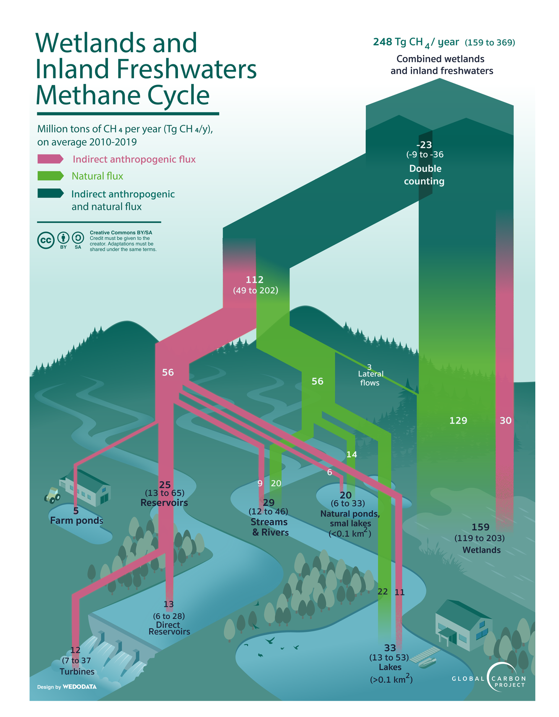
Figure 4Estimation of wetland and inland freshwater emissions over the 2010–2019 decade (in Tg CH4 yr−1). The fluxes related to voluntary (such as through reservoirs or farm ponds) or involuntary (land use or eutrophication-related) perturbations of the methane cycle are shown here in pink. They are accounted for in the “natural and indirect anthropogenic” sources in the Table 3 budget and depicted as “natural and indirect anthropogenic” sources (darker green and pink hatches) in Fig. 7. Infographic designed by WeDoData (https://wedodata.fr, last access: 1 April 2025).
Lakes and ponds
The previous global CH4 budget used an estimate of 71 Tg CH4 yr−1 for lakes and 18 Tg CH4 yr−1 for reservoirs. These estimates were based on an early study by Bastviken et al. (2011) coupled with a newer estimate for lakes north of 50° N (Wik et al., 2016b). There have been three new lake studies that have published their data with global estimates of 56 and 151 ± 73 (Rosentreter et al., 2021; respectively for the median and mean ± CI 95 %, 22 ± 8 (Zhuang et al., 2023; ± lake-area-weighted normalised RMSE for all parameterised lake types), process-based model) and 41 ± 36 Tg CH4 yr−1 (Johnson et al., 2022a, mean ± CI 95 %). This large range in estimated emissions can be attributed to the differences in the data sets and methods used to calculate the surface area of small waterbodies, as well as the differences between how the flux data were analysed and extrapolated between studies. For instance, total surface areas of all lakes and ponds of 3712–5688 × 103 km2 (Rosentreter et al., 2021) and 2806 × 103 km2 (Johnson et al., 2022a) were used along with measurement data from 198 and 575 individual lake systems respectively. In contrast, Zhuang et al. (2023) generated estimates using higher-temporal-resolution data from just 54 lakes to build a process-based model, which generated much lower flux estimates from tropical lakes than previously implemented statistical approaches, but in line with the most recent assessments by Borges et al. (2022). For this study, we explicitly excluded lakes < 0.1 km2, which are treated separately (see below). If we re-assess these three studies for only lakes greater than 0.1 km2, we obtain global effluxes of 17 and 42.9 ± 20.8 Tg CH4 yr−1 (Rosentreter et al., 2021; median and mean ± CI 95 % of global flux), 21.9 ± 8.0 (Zhuang et al., 2023, ± lake-area-weighted normalised RMSE for all parameterised lake types), and 35.3 ± 31.0 Tg CH4 yr−1 (Johnson et al., 2022a, b, ±95 % CI) (with areas of 2556–3468 × 103, 2640×103, and 2676×103 km2 respectively). Thus, for lakes > 0.1 km2, we propose an efflux of 33 ± 26 Tg CH4 yr−1 (an average of the mean from Rosentreter et al., 2021, Zhuang et al., 2023, and Johnson et al., 2022a, b, with the average CI 95 % from Rosentreter et al., 2021, and Johnson et al., 2022a, b) as represented in Fig. 4. Small waterbody emissions, hereafter small lakes and ponds < 0.1 km2, remain difficult to assess. Evidence is emerging that there is a lower limit to the power scaling laws that early studies used to extrapolate the surface area of these small systems (Bastviken et al., 2023; Kyzivat et al., 2022). Thus, for small lakes and ponds < 0.1 km2 (and > 0.001 km2), we disregard the higher end surface area used in Rosentreter et al. (2021), which relied on these earlier estimates and scale their numbers to the evasion estimates to the lower-end surface area of 1002×103 to obtain a mean flux of 33 Tg CH4 yr−1 (Rosentreter et al., 2021). Johnson et al. (2022a) estimated a surface area of only 166×103 km2 for this size class to obtain an efflux of 6.3 Tg CH4 yr−1, which we acknowledge as a lower limit. Averaging these two values provides a conservative estimate of 20 [6–33] Tg CH4 yr−1, which is close to the number proposed by Holgerson and Raymond (2016) for diffusion effluxes only for this size class. The experts involved in this assessment have low confidence in this estimate. This estimate also does not include artificial ponds, which we discuss below. As a result, combined CH4 emissions from large lakes (> 0.1 km2) and small lakes and ponds (< 0.1 km2) are estimated at 53 [19–86] Tg CH4 yr−1 (Fig. 4), which is lower than the 71 Tg estimated in the previous budget.
Reservoirs
New mean estimates of diffusive + ebullition CH4 emissions from reservoirs include 15 and 24 ± 8 (the median and mean ± CI 95 % from Rosentreter et al., 2021), 10 ± 4 (Johnson et al., 2021, mean ± 95 % CI), 10 (Harrison et al., 2021, low and high 95 % CI of 7 and 22 respectively), and 2.1 Tg CH4 yr−1 (Zhuang et al., 2023). We compile the first three estimates to a direct efflux of ∼ 14 Tg CH4 yr−1 (with ± CI 95 % of 9 and 23). We note the fourth estimate as a lower bound but exclude it from this budget given that it was generated via a model that only included data from six reservoir systems (Zhuang et al., 2023). We also add in an additional 12 Tg CH4 yr−1 (low and high 95 % CI of 7 and 37 respectively) that is estimated to degas in dam turbines (Harrison et al., 2021), which was not addressed in the studies by Rosentreter et al. (2021), Zhuang et al. (2023), or Johnson et al. (2021). Rocher-Ros et al. (2023) also excluded river observations below dams when executing their statistical model and so did not capture downstream dam emissions. Thus, we use a direct reservoir emission here of ∼ 13 [6–28] Tg CH4 yr−1 and estimate an additional ∼ 12 [7–37] Tg CH4 yr−1 from dam turbine degassing fluxes, giving a total of 25 [13–65] Tg CH4 yr−1 from reservoirs (Fig. 4).
Uncertainties and confidence levels
The emission estimates of lakes, reservoirs, and ponds described above are limited by several uncertainties. First, a major unknown for lakes remains the size cut-off and the representation of small lakes and ponds (Deemer and Holgerson, 2021), which are also more variable than larger water bodies in their CH4 concentrations and fluxes (Rosentreter et al., 2021; Ray et al., 2023). Interestingly, there is also a lack of methane data representation from large lakes that are a large component of global lake surface area (Deemer and Holgerson, 2021; Messager et al., 2016). There is also a growing knowledge base on the importance of high CH4 fluxes from lake littoral zones that is not yet well incorporated into global scaling efforts (e.g. Grinham et al., 2011; Natchimuthu et al., 2016) and emergent vegetation (Bastviken et al., 2023; Kyzivat et al., 2022). Ebullition is more constrained in lakes/reservoirs compared to streams/rivers but is still difficult to measure and model accurately. Finally, for all inland water systems a greater scrutiny for the limiting factors (including the impact of ice cover and seasonality, stratification of the water column) of different CH4 production, consumption, and transport pathways is needed. In addition, a better understanding of the climatic, environmental, and geomorphological controls on key CH4 processes (e.g. sedimentary diffusive and ebullition production, bubble dissolution, CH4 oxidation) on the large-scale remains critically needed. For instance, the consistently lower global emissions determined by the process-based model of Zhuang et al. (2023) compared to observations suggest that current data sets are too limited to fully capture the spatiotemporal variability in CH4 dynamics and their key control factors, possibly leading to biased-high estimates.
The majority of the inland water CH4 estimates are from a limited number of studies, some without spatial representation or reported statistical uncertainties. Furthermore, as mentioned above the knowledge base of the surface area of these ecosystems is new and rapidly expanding but not standardised between studies leading to uncertainty (but see Lauerwald et al., 2023b), particularly for ponds. For this study, we are able to provide confidence intervals from the original studies for all fluxes except the smallest lake/pond size class.
The surface area of inland freshwaters
For all of these ecosystems, determining their surface area remains a central challenge. Since the last GMB, several methodological advances have reduced the uncertainty associated with the surface area estimates of rivers, streams, lakes, and reservoirs. Using a single geospatial data set that includes both lakes and reservoirs (Messager et al., 2016) has decreased double counting of lakes and reservoirs (Johnson et al., 2022a; Rosentreter et al., 2021). For rivers and streams, high-resolution global streamflow simulations, informed by satellite observations, enabled a much finer-scale estimate of surface areas for rivers with a new temporal component (Allen and Pavelsky, 2018; Lin et al., 2019; Liu et al., 2022), although the surface for the smaller streams are still estimated indirectly, and mapping of human-created drainage ditches and canals is lacking. Seasonal ice cover and melt turnover corrections also have been newly incorporated into rivers, streams, lakes, and reservoirs (Harrison et al., 2021; Johnson et al., 2022a; Lauerwald et al., 2023b; Rocher-Ros et al., 2023; Rosentreter et al., 2021; Zhuang et al., 2023). Finally, removing open-water-body surface areas from wetland surface areas based on geographic location has reduced double counting between these two land cover types, as described in the wetlands section of the GMB. However, the surface area of small lakes and ponds (< 0.1 km2) is still highly uncertain, and new techniques for counting these systems and determining the overlap with wetland data bases are paramount.
Anthropogenic contributions to inland freshwater emissions
We argue that all reservoirs should be categorised as a direct anthropogenic source of emissions. Most of the surface area of reservoirs are human-made, and reservoir construction leads to anoxic sediments and/or bottom waters with labile organic matter sourced from the watershed and to in situ nutrient augmented phytoplankton production (Deemer et al., 2016; Maavara et al., 2017; Prairie et al., 2018). It is also clear that the cultural eutrophication of natural lakes driven by run-off of agricultural nitrogen fertiliser and manure augments CH4 emissions (DelSontro et al., 2018; Li et al., 2021), with shallow lakes particularly likely to experience eutrophication (Qin et al., 2020). For instance, Beaulieu et al. (2019) modelled a 15 % reduction in lake CH4 with a 25 % reduction in lake phosphorus concentrations. Several recent studies have estimated that anywhere between 30 % and 50 % of lakes are eutrophic (Cael et al., 2022; Qin et al., 2020; Sayers et al., 2015; Wu et al., 2022). These studies estimate numerical percentages (one by depth class: Qin et al., 2020), but none have estimated the percent of lake surface area that is eutrophic nor have any determined the extent of anthropogenic vs. natural eutrophication. Still, numerous studies have noted widespread increases in eutrophication indicators across lakes due to nutrient loading and warming (Griffiths et al., 2022; Ho et al., 2019; Taranu et al., 2015); thus we estimate that one-third or 11 Tg CH4 yr−1 of CH4 emissions from lakes > 0.1 km2 could be anthropogenic (Fig. 4). Similarly, CH4 emissions from small lakes and ponds are influenced by human factors, with emissions increasing with eutrophication (Deemer and Holgerson, 2021), erosion and runoff in agricultural landscapes (Heathcote et al., 2013), and warming, the latter likely to have a disproportionately greater effect in small, shallow systems (Woolway et al., 2016). Thus, we adopt the same number as for lakes for the proportion of anthropogenic emissions in small lakes and ponds (< 0.1 km2), which amounts to 6 Tg CH4 yr−1 (Fig. 4).
There are also human-made small lakes and ponds, notably for agriculture, aquaculture, and recreation, that generally have conditions favourable for high CH4 emissions (Downing, 2010; Holgerson and Raymond, 2016; Malerba et al., 2022; Ollivier et al., 2019; Zhao et al., 2021; Dong et al., 2023). Downing (2010) estimated that farm ponds comprise a global surface area of ∼ 77 000 km2; using a conservative emission rate of 265 mg CH4 m−2 d−1 and an ice correction factor of 0.6 leads to an emission of 4.5 Tg yr−1 that is anthropogenically sourced from farm ponds. Here the value is rounded to 5 Tg yr−1 (Fig. 4). Clearly, more work is required to assess the anthropogenic component of CH4 emissions from lakes and ponds.
It remains difficult to parse out an anthropogenic component to stream and river CH4 fluxes. Although some studies have noticed a temperature dependence with stream sediments (Comer-Warner et al., 2018; Zhu et al., 2020), Rocher-Ros et al. (2023) noted a small temperature dependence of CH4 emissions in streams and rivers compared to other freshwater ecosystems, potentially due to the many other external processes affecting fluxes in these dynamic flowing ecosystems. Urbanisation can lead to elevated river CH4 emissions, particularly in regions with elevated organic matter and nutrient loading due to limited wastewater treatment (Begum et al., 2021; Nirmal Rajkumar et al., 2008; Wang et al., 2021a). Some studies have found agricultural streams and ditches can have higher effluxes due to inputs of fine sediments (Comer-Warner et al., 2018; Crawford and Stanley, 2016), organic carbon, and nutrients (Borges et al., 2018) that lead to in situ methane production. Furthermore, the creation of drainage ditches in organic soils taps CH4-rich waters from water-logged horizons and increases the emissions from ex situ sources (Peacock et al., 2021). However, limitations in both the geographic coverage of existing ditch emission estimates and our ability to estimate the global surface area of ditches preclude their inclusion in this budget. Finally, extremely high rates of CH4 emission have been linked to ongoing permafrost thaw in Asia's Qinghai–Tibet Plateau (Zhang et al., 2020). However, the loss and disconnection of wetlands to rivers may have resulted in a decrease in the input of dissolved CH4 from this source. A recent expert elicitation (Rosentreter, et al., 2024) reported that 35 % of all inland freshwater sources were anthropogenic; given that some of the river flux is from upstream reservoirs, we assign a 30 % anthropogenic contribution to the stream and river flux (9 Tg CH4 yr−1, Fig. 4), which approximates the expert elicitation via the impact of eutrophication and urban influences.
Combination (lakes, ponds, reservoirs, streams and rivers, farm ponds)
Combining the aforementioned emissions from lakes > 0.1 km2 (33 [13–53] Tg CH4 yr−1), small lakes and ponds < 0.1 km2 (20 [6–33] Tg CH4 yr−1), reservoirs (25 [13–65] Tg CH4 yr−1), streams and rivers (29 [12–46] Tg CH4 yr−1) and farm ponds (5 Tg CH4 yr−1) leads to a total of ∼ 112 Tg CH4 yr−1 from freshwater systems, with a range of [49–202] Tg CH4 yr−1. This estimate is about 50 Tg lower than in Saunois et al. (2020) and is broadly consistent with the recent regionalised estimate by Lauerwald et al. (2023b) compiled for the Regional Carbon Cycle Assessment and Processes (RECCAP2, https://www.globalcarbonproject.org/reccap/, last access: 1 April 2025; 103 Tg CH4 yr−1, IQR = 82.1–134.8). The updated budget from these ecosystems and their anthropogenic components are represented in Fig. 4. The gridded products for emissions from lakes and ponds by Johnson et al. (2022b), from reservoirs by Johnson (2021), and from streams and rivers by Rocher-Ros (2023) have been combined into a single map presented in Fig. 5.
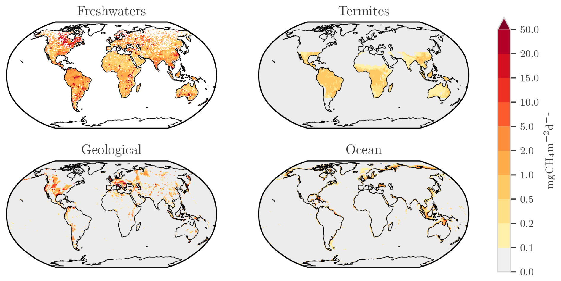
Figure 5Methane emissions (mg CH4 m−2 d−1) from four natural and indirect anthropogenic sources: inland freshwaters (including lakes, ponds (Johnson et al., 2022b), reservoirs (Johnson et al., 2021; Johnson, 2021), and stream and rivers (Rocher-Ros et al., 2023; Rocher-Ros, 2023) with a global total scaled to 89 Tg yr−1), geological sources (Etiope et al., 2019), termites (this study), and oceans (Weber et al., 2019).
Double counting inland freshwater ecosystems in the bottom-up estimates
To address the differences found between bottom-up and top-down CH4 budgets, and to acknowledge advances in addressing the central issue of double counting CH4 emissions for inland freshwater ecosystems, we introduce here a new correction term. Historically, the bottom-up estimate of global CH4 emissions has been higher than the top-down estimate, first recognised in Kirschke et al. (2013) and confirmed in Saunois et al. (2016, 2020). The larger bottom-up emissions estimate has been partly attributed to double counting vegetated wetland emissions with inland freshwater emissions (including lakes, ponds, rivers, streams, and reservoirs) and the emissions of CH4 produced in vegetated wetlands and then transported via aquatic processes and emitted from inland freshwaters (Pangala et al., 2017; Kirk and Cohen, 2023). The Saunois et al. (2020) CH4 budget addressed the issue of double counting through the use of a revised vegetated wetland area data set, WAD2M v1.0 (Zhang et al., 2021a), which removed inland waters from the SWAMPS (Jensen and McDonald, 2019) surface–inundation data set, allowing for independent vegetated wetlands and inland freshwater CH4 emissions to be compiled. However, the Saunois et al. (2020) CH4 budget still had a ∼ 150 Tg CH4 yr−1 difference between bottom-up and top-down estimates. In this budget, we refined the vegetated wetland area data set with WAD2M v2.0 (see Sect. 3.2.1, where HydroLAKES is used to remove lakes and ponds > 0.1 km2). Additionally, we applied numbers from peer-reviewed publications and expert elicitation to account for lateral CH4 flux emissions. This most recent bottom-up budget estimates 159 [119–203] Tg CH4 yr−1 from vegetated wetlands for 2010–2019 and 112 Tg CH4 yr−1 from inland freshwaters, which includes 83 Tg CH4 yr−1 from lakes, ponds, and reservoirs and 29 Tg CH4 yr−1 from rivers and streams, leading to a combined wetland and inland freshwater flux of 271 Tg CH4 yr−1. Here, we propose a correction of 20 Tg CH4 yr−1 to account for double counting of small lakes and ponds (< 0.1 km2) that are likely included in our vegetated wetlands estimate and removing 1–3 Tg CH4 yr−1 from river emissions due to lateral transport of CH4 originating in adjacent vegetated wetlands. The river flux correction arises from assuming that for catchments with > 10 % wetlands, rivers provide 5 %–10 % of vegetated CH4 emissions. The total double counting correction term of 23 Tg CH4 reduces the bottom-up budget for combined wetlands and inland waters from 271 to 248 Tg CH4 yr−1 (see Fig. 4 and Table 3). Comparing the 2000–2009 decadal emissions from wetlands and inland freshwater ecosystems across the last three previous assessments of the budget shows a significant downward revision with 305 (183 + 122) Tg CH4 yr−1, 356 (147 + 209) Tg CH4 yr−1 and 248 (159 + 112 − 23) Tg CH4 yr−1 (respectively from Saunois et al. 2016, 2020, and this work).
Finally, it is worth noting that inland freshwater ecosystems can overlap with geological seepage systems in some areas; i.e. they may occur in correspondence with geological structures that emit fossil (microbial, thermogenic, or abiotic) CH4 generated in the Earth's crust. Examples have been documented in the Fisherman Lake in Canada (Smith et al., 2005), in Lake Baikal (Schmid et al., 2007), and in rice paddies in Japan (Etiope et al., 2011). Thus, some gas emissions in freshwater environments, particularly as bubble plumes, can be incorrectly attributed to modern biological (ecosystem) activities if appropriate isotopic and molecular analyses are not performed.
3.2.3 Onshore and offshore geological sources
Significant amounts of CH4, produced within the Earth's crust, naturally migrate to the atmosphere through tectonic faults and fractured rocks. Major emissions are related to hydrocarbon formation in sedimentary basins (microbial and thermogenic methane), through continuous or episodic exhalations from onshore and shallow marine hydrocarbon seeps and through diffuse soil microseepage (Etiope, 2015). Specifically, five source categories have been considered. Four are onshore sources: gas–oil seeps, mud volcanoes, diffuse microseepage, and geothermal manifestations including volcanoes. One source is offshore: submarine seepage, which may include the same types of gas manifestations occurring on land. Etiope et al. (2019) have produced the first gridded maps of geological CH4 emissions and their isotopic signature for these five categories, with a global total of 37.4 Tg CH4 yr−1 (reproduced in Fig. 5). However, these maps are based on incomplete data on geological sites due to missing information and difficulties in defining all current geological emitting sites. Combining the best estimates for the five categories of geological sources (from grid maps or from previous statistical and process-based models), the breakdown by category reveals that onshore microseepage dominates (24 Tg CH4 yr−1), with the other categories having similar smaller contributions: as mean values, 4.7 Tg CH4 yr−1 for geothermal manifestations, about 7 Tg CH4 yr−1 for submarine seepage, and 9.6 Tg CH4 yr−1 for onshore seeps and mud volcanoes. These values lead to a global bottom-up geological emission mean of 45 [27–63] Tg CH4 yr−1 (Etiope and Schwietzke, 2019).
While all bottom-up and some top-down estimates, following different and independent techniques from different authors, consistently suggest a global geo-CH4 emission on the order of 40–50 Tg yr−1, the radiocarbon (14C–CH4) data in ice cores reported by Hmiel et al. (2020) appear to give a much lower estimate, with a minimum of about 1.6 Tg CH4 yr−1 and a maximum value of 5.4 Tg CH4 yr−1 (95 % confidence) for the pre-industrial period. Dyonisius et al. (2020) also suggest a low range of geological emissions over the last deglaciation period and for the Late Holocene (0–10 Tg CH4 yr−1). The discrepancy between Hmiel et al. (2020) and all other estimates has been discussed in Thornton et al. (2021), which demonstrated that the global near-zero geologic CH4 emission estimate in Hmiel et al. (2020) is incompatible with the sum of multiple independent bottom-up estimates, based on a wide variety of methodologies, from individual natural geological seepage areas: for example, from the Black Sea (up to 1 Tg CH4 yr−1), the Eastern Siberian Arctic Shelf (ESAS; up to 4.6 Tg CH4 yr−1, referring mostly to thermogenic gas), onshore Alaska (up to 1.4 Tg CH4 yr−1), and a single seepage site in Indonesia (releasing 0.1 Tg CH4 yr−1 as estimated by satellite measurement) (see Thornton et al., 2021, and references therein). Jackson et al. (2020) expressed doubt about the low Hmiel et al. (2020) estimates, noting that they are difficult to reconcile with the results of many other researchers and with bottom-up approaches in general. This discrepancy highlights another main unresolved uncertainty in the methane budget and calls for further investigations to reconcile the different estimates and reduce the uncertainty on geological emissions. Waiting for further investigation to better understand discrepancies between radiocarbon approaches and other studies, we decided to keep the estimates from Etiope and Schwietzke (2019) for the mean values and associate them with the lowest estimates reported in Etiope et al. (2019), as in Saunois et al. (2020). Thus, we report a total global geological emission of 45 [18–63] Tg CH4 yr−1, with a breakdown between offshore emissions of 7 [5–10] Tg CH4 yr−1 and onshore emissions of 38 [13–53] Tg CH4 yr−1 (Table 3), similar to Saunois et al. (2020). This bottom-up estimate is slightly lower than in the Saunois et al. (2016) budget mostly due to a reduction of estimated emissions of onshore and offshore seeps (see Sect. 3.2.6 for more offshore contribution explanations).
Table 4Top-down studies used here with their contribution to the decadal and yearly estimates noted. For decadal means, top down studies must provide at least 8 years of data over the decade to contribute to the estimate. Details on each inverse system and inversions are provided in Tables S8 to S11 in the Supplement.
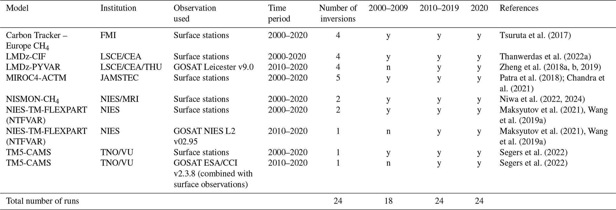
Table 5Global and latitudinal total methane emissions (in Tg CH4 yr−1), as decadal means (2000–2009 and 2010–2019) and for the year 2020 from this work using bottom-up and top-down approaches. Global and latitudinal emissions for 2000–2009 are also compared with Saunois et al. (2016, 2020) for top-down and bottom-up approaches when available. Uncertainties are reported as [min–max] range. The mean, minimum, and maximum values are calculated while discarding outliers, for each category of source and sink. As a result, discrepancies may occur when comparing the sum of categories and their corresponding total due to differences in outlier detections. Differences of 1 Tg CH4 yr−1 in the totals can also occur due to rounding errors. For the latitudinal breakdown, bottom-up anthropogenic estimates are based only on the gridded products (see Table 1). As a result, the total from the latitudinal breakdown (line called “This work (gridded BU products only”)) is slightly different from the values provided in Table 3 and recalled in the line “This work (all BU products)”. BU stands for bottom-up. S2020 and S2016 refer to Saunois et al. (2020) and Saunois et al. (2016) respectively.
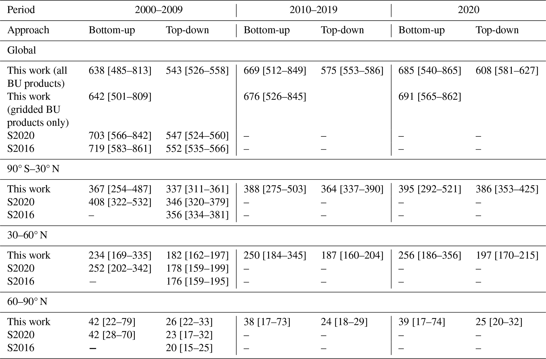
3.2.4 Termites
Termites are decomposers playing a central role in ecosystem nutrient fluxes at tropical and subtropical latitudes, in particular (Abe et al., 2000). Termites represent a natural CH4 source due to methanogenesis occurring in their hindgut during the symbiotic metabolic breakdown of lignocellulose (Sanderson, 1996; Brune, 2014). The upscaling of CH4 emissions from termites from site to global level is characterised by high uncertainty (Sanderson, 1996; Kirschke et al., 2013; Saunois et al., 2016) due to the combination of factors that need to be considered and the scarcity of information for each of these factors for global upscaling. Needed data include termite biomass density (Sanderson, 1996), species distribution within and among ecosystems (Sugimoto et al., 1998), variation in termite CH4 emission rates per species and dietary group (Sanderson, 1996), and the role played by the termite mound structure in affecting the fraction of produced CH4 that is effectively released into the atmosphere (Sugimoto et al., 1998; Nauer et al., 2018). In Kirschke et al. (2013) and Saunois et al. (2016), a global upscaling of termite CH4 emissions was proposed, where CH4 emissions, (kg CH4 ha−1 yr−1), were estimated as the product of three terms: termite biomass (BioTERM g fresh weight m−2), a scalar correction factor (LU) expressing the effect of land use/cover change on termite biomass density, and a termite CH4 emission factor (EFTERM, µg CH4 g−1 BioTERM h−1). The approach between the two re-analyses of CH4 emissions varied only for the data sources of gross primary productivity (GPP) and land use, which were used to attribute biomass values of termite per ecosystem surface unit, in order to cover different time spans: 1980s, 1990s, and 2000s in Kirschke et al. (2013) and 2000–2007 and 2010–2016 in Saunois et al. (2016). For the present update, additional changes have been introduced compared with the previous versions. Here we summarise the key data used for the new upscaling. CH4 fluxes were modelled between 45° S and 45° N and within 35° S and 35° N. The termite biomass density, BioTERM, for tropical ecosystems was estimated as a function (Kirschke et al., 2013; Bio)) of the gross primary production (GPP; g C m−2 yr−1) using the 0.25° native resolution VODCA2GPP data set covering the period 2001–2020 (Wild et al., 2022). Wetlands, barren areas, water bodies, and artificial surfaces were excluded from this estimation and set as no data (no emissions). The scalar correction factor LU of 0.4 (60 %) for agricultural areas (i.e. croplands) (Kirschke et al., 2013) was applied to the GPP value of the nearest natural areas to account for anthropic disturbance. The annual (2001–2020) land cover information was obtained from the MODIS Terra+Aqua Combined Land Cover product (MCD12C1v006; https://lpdaac.usgs.gov/products/mcd12c1v006/, last access: 1 April 2025), using the International Geosphere-Biosphere Programme (IGP) classification with a 0.05° spatial resolution. For desert and arid lands, within 35° S and 35° N, a fixed BioTERM value of 1.56 g m−2 was instead used (Sanderson, 1996; Heděnec et al., 2022). Similarly, fix values from the few available studies reported in literature were used to estimate BioTERM between 35–45° N and 35–45° S as follows: 1.83 g m−2 for temperate forests and grasslands (Wood and Sands, 1978; Petersen and Luxton, 1982; Sanderson, 1996; Bignell and Eggleton, 2000; King et al., 2013; conversion factor from dry to fresh biomass is 0.27 from Petersen and Luxton, 1982), 5.3 g m−2 for shrublands and Mediterranean areas of Australia (Sanderson, 1996), and 1.09 g m−2 for the other Mediterranean shrubland ecosystems (Heděnec et al., 2022). Other climates and land covers were set as no data. Climate zoning was defined using the Köppen–Geiger climate zone data set (Beck et al., 2018); this product is representative of the 1980–2016 time period and has a 0.0083° native resolution. The EFTERM was revised compared with previous estimates (Kirschke et al., 2013; Saunois et al., 2016), in order to consider the different distribution of termite families and subfamilies in the different continents and ecosystems, characterised by different feeding habits and nest typologies, as reported by Sugimoto et al. (1998), which might influence the EF. The species of each family and subfamily of the two major groups of lower and higher termites, listed by Sugimoto et al. (1998), were associated with EF values based on emissions from in vitro experiments as reported by Sanderson (1996) and Eggleton et al. (1999), to which a correction factor (cfMOUND) of 0.5 (Nauer et al., 2018; Chiri et al., 2020, 2021) was applied in order to take into account the mound effect on the CH4 produced by termites, once inside the nest. The average EFTERM for tropical and temperate areas was hence estimated as the weighted EFTERM derived from the product of the percentage weight of each family or subfamily of termites in the “community composition” in each geographical area and ecosystem (Sugimoto et al. (1998; Table 6), the respectively calculated EF of each family or subfamily, and a scalar or correction factor which considers the nest type (as in Table 5 from Sugimoto et al., 1998). For desert and arid lands and temperate areas, which were not reported in Sugimoto et al. (1998), EF rates were calculated directly from data reported in literature for the most representative species, which were the genus Amitermes for the former (EF from data by Sanderson, 1996; Eggleton et al., 1999; Jamali et al., 2011) and the genus Reticulitermes (family Rhinotermitidae) for the latter (EF from data by Odelson and Breznak, 1983; Sanderson, 1996; Eggleton et al., 1999; Myer et al., 2021). The following EFTERMs were hence obtained to scale up emissions: 3.26 ± 1.79 µg CH4 g−1 termite h−1 (28.56 mg CH4 g−1 termite yr−1) for tropical ecosystems; 1.82 ± 1.54 µg CH4 g−1 termite h−1 for temperate forests, grasslands, and Mediterranean areas; and 1.24 ± 1.22 µg CH4 g−1 termite h−1 for deserts and arid lands (warm climate). Annual CH4 fluxes were computed for all the years from 2001 to 2020, producing 20 global maps at 0.05° resolution of yearly total emissions. A further map of the estimated error representative of the entire time period was elaborated at the same resolution as the emissions data set.
Table 6Latitudinal methane emissions (in Tg CH4 yr−1) for the last decade 2010–2019, based on top-down and bottom-up approaches. Uncertainties are reported as [min–max] range of reported studies. The mean, minimum, and maximum values are calculated while discarding outliers, for each category of source and sink. As a result, discrepancies may occur when comparing the sum of categories and their corresponding total due to differences in outlier detections. Differences of 1 Tg CH4 yr−1 in the totals can also occur due to rounding errors. For bottom-up approaches, natural and indirect anthropogenic sources are estimated based on available gridded data sets (see text Sect. 5.2). As some emissions are missing gridded products (wild animals, permafrost, and hydrates), discrepancies may occur in terms of totals proposed in Table 3. Bottom-up direct anthropogenic estimates are based only on the gridded products (see Table 1).
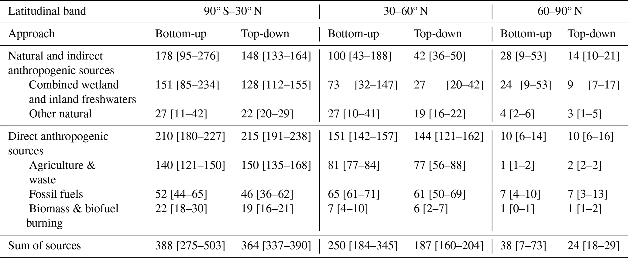
Termite CH4 emissions over the period 2001–2020 varied between 9.7–10.8 Tg CH4 yr−1, with an average of 10.2 ± 6.2 Tg CH4 yr−1. Considering a 20-year average, tropical and subtropical moist broadleaf forests contributed to 46 % of the total average flux, while tropical and subtropical grasslands, savannas, and shrublands to another 36 %. In terms of regional contribution, 37.2 % of fluxes were attributed to South America, 31.5 % to Africa, 18.1 % to Asia, 5.5 % to Australia, 7.4 % to North America, and less than 1 % to Europe. The present estimate value is within the range of previous upscaling studies, spanning from 2 to 22 Tg CH4 yr−1 (Ciais et al., 2013). In this study, we report a decadal value of 10 Tg CH4 yr−1 with a range of [4–16] (Table 3).
3.2.5 Wild animals
Wild ruminants emit CH4 through microbial fermentation that occurs in their rumen, similarly to domesticated livestock species (USEPA, 2010b). Using a total animal population of 100–500 million, Crutzen et al. (1986) estimated the global emissions of CH4 from wild ruminants to be in the range of 2–6 Tg CH4 yr−1. More recently, Pérez-Barbería (2017) lowered this estimate to 1.1–2.7 Tg CH4 yr−1 using a total animal population estimate of 214 million (range of 210–219), arguing that the maximum number of animals (500 million) used in Crutzen et al. (1986) was poorly justified. Moreover Pérez-Barbería (2017) also stated that the value of 15 Tg CH4 yr−1 found in the last IPCC reports is much higher than their estimate because this value comes from an extrapolation of Crutzen's work for the last glacial maximum when the population of wild animals was much larger, as originally proposed by Chappellaz et al. (1993). Recently, based on the modelling of grassland extent, Kleinen et al. (2023) also suggest that the populations of wild animals during the last glacial maximum proposed by Crutzen et al. (1986) and further used by Chappellaz et al. (1993) were overestimated. However, the estimate of 1–3 Tg CH4 yr−1 seems underestimated when considering that Hempson et al. (2017) found actual CH4 emissions from African wildlife alone to be around 9 Tg CH4 yr−1 but without discussing the uncertainty of this value. As a result, high uncertainty remains and recalls the need for further investigation of this natural source of CH4.
Based on these findings and waiting for further global estimates, the range adopted in this updated CH4 budget is 2 [1–3] Tg CH4 yr−1 (Table 3).
3.2.6 Coastal and oceanic sources
Coastal and oceanic sources comprise CH4 release from estuaries, coastal vegetated habitats, and marine waters, including seas and oceans. Possible sources of coastal and oceanic CH4 include (1) in situ biogenic production through various pathways in oxygenated sea surface waters (Oremland, 1979; Karl et al., 2008; Lenhart et al., 2016; Repeta et al., 2016), a flux that can be enhanced in the coastal ocean because of submarine groundwater discharge (USEPA, 2010b); (2) production from shallow and marine (bare and vegetated) sediments including free gas or destabilised hydrates and thawing subsea permafrost containing modern (14C-bearing) microbial gas; and (3) geological marine seepage (see also Sect. 3.2.3), including hydrates, containing fossil (14C-free) microbial or thermogenic CH4. CH4 produced in marine sediments and seabed CH4 seepage can be transported across the water column to the sea surface by upwelling waters (once at the surface methane can cross the sea–air interface via diffusion) and gas bubble plumes (for instance from geological marine seeps; e.g. Judd, 2004; Etiope et al., 2019). Gas bubble plumes generally reach the atmosphere in relatively shallow waters (< 400 m) of continental shelves depending on the intensity of the events (e.g. Westbrook et al., 2009); however massive deep-water seepage events could contribute a significant amount of CH4 to the atmosphere, even from depths > 1000 m (e.g. Schmale et al., 2005.; Greinert et al., 2006; Solomon et al., 2009). In coastal vegetated habitats, CH4 can also be transported to the atmosphere through the aerenchyma of emergent aquatic plants (Purvaja et al., 2004).
We distinguish between coastal and oceanic “geological” and “modern biogenic” CH4 sources. Coastal and oceanic “geological” emissions refer to CH4 seepage from the Earth's crust (mostly in hydrocarbon-rich sedimentary basins), which is typically evaluated by combining geochemical analyses (isotopic and molecular, including radiocarbon, 14C, analyses) and geological observations (degassing along faults, seeps, mud volcanoes). Geological emissions do not contain modern biogenic gas that is fossil (14C-free). Coastal and oceanic “biogenic” CH4 refers to CH4 formed in situ in coastal and marine sediments and in the water column by recent or modern microbial activity (therefore with measurable amounts of radiocarbon (14C)). To avoid double counting, we assume that all diffusive CH4 emissions outside of geological seepage regions (identified in global grid maps; Etiope et al., 2019) are fuelled by biogenic CH4. Finally, we briefly discuss the case of CH4 hydrates, which can be considered either a “geological” source when they host fossil CH4 or a “biogenic” source when they host modern CH4.
Coastal and oceanic modern biogenic methane emissions
Area-integrated diffusive modern biogenic CH4 emissions from coastal ecosystems are 1–2 magnitudes lower than from inland freshwaters but significantly higher than biogenic emissions from the open ocean (Rosentreter et al., 2021; Rosentreter et al., 2023; Weber et al., 2019). Particularly the shallow vegetated coastline fringed by mangroves, salt marshes, and seagrasses is a CH4 hotspot in the coastal ocean, characterised by significantly higher flux densities than other coastal settings such as estuaries or the continental shelves (Rosentreter et al., 2021; Rosentreter et al., 2023). Coastal ecosystems are thus being increasingly recognised as weak global sources to the atmosphere (Weber et al., 2019; Saunois et al., 2020; Rosentreter et al., 2021). Hydrogenotrophic and acetoclastic methanogenesis are largely outcompeted by sulfate reduction in coastal/marine sediments, which is often shown by a decreasing trend of CH4 concentrations with increasing salinity from upper tidal (low salinity) to marine (high salinity) regions. Much of the CH4 produced below the sulfate-reduction zone is indeed re-oxidised by sedimentary anaerobic methane oxidation or re-oxidised in the water column, leading to small emissions despite much larger production (Knittel and Boetius, 2009; Regnier et al., 2011). Methylated compounds such as methylamines and methyl sulfides are non-competitive substrates that are exclusively used by methanogens; therefore, methylated methanogenesis can occur in coastal regions with high sulfate concentrations, for example, in organic-rich (Maltby et al., 2018), vegetated (Schorn et al., 2022), and hypersaline coastal sediments (Xiao et al., 2018). Coastal CH4 can be driven by the exchange of pore water or groundwater (high in CH4) with coastal surface waters in tidal systems, referred to as tidal pumping (Ovalle et al., 1990; Call et al., 2015). Anthropogenic impacts such as wastewater pollution and land use change can increase CH4 fluxes in estuaries (Wells et al., 2020). A large increase of CH4 emissions follows the conversion of natural coastal habitats to aquaculture farms (Yuan et al., 2019; Yang et al., 2022).
Currently available global modern biogenic CH4 flux data show high spatiotemporal variability within and between coastal systems because of the overall global paucity of data. Therefore, global estimates have high uncertainties and show large ranges in both empirical (Rosentreter et al., 2021) and machine-learning-based approaches (Weber et al., 2019). According to a recent data-driven metadata analysis, global estuaries, including tidal systems and deltas, lagoons, and fjords, are estimated to emit a median (Q1–Q3) of 0.25 (0.07–0.46) Tg CH4 yr−1 (Rosentreter et al., 2023). Coastal vegetation, including mangrove forests, salt marshes, and seagrasses, is estimated to emit 0.77 (0.47–1.41) Tg CH4 yr−1, which is 3 times more than global estuaries (Rosentreter et al., 2023). The combined median (Q1–Q3) emission of 1.01 (0.54–1.87) Tg CH4 yr−1 for coastal vegetation and estuaries by Rosentreter et al. (2023) is lower than the recent observation-based global synthesis including tidal flats and aquaculture ponds (median 1.49 (0.22–6.48) Tg CH4 yr−1) by Rosentreter et al. (2021). Total shallow coastal modern biogenic CH4 emissions based on existing data including emissions from estuaries, coastal vegetation (Rosentreter et al., 2023), tidal flats, and human-made coastal aquaculture ponds (Rosentreter et al., 2021) amount to a median (Q1–Q3) of 1.8 (0.59–5.57) Tg CH4 yr−1. This range is about 3–4 times lower than the earlier global assessment by Borges and Abril (2011) and also lower than the value of 4–5 Tg CH4 yr−1 reported in the previous CH4 budget for inner and outer estuaries including marshes and mangroves (Saunois et al., 2020), which was based on a significantly smaller data set (n=80) and larger estuarine surface areas (Laruelle et al., 2013) than used here (Laruelle et al., 2025).
The nearshore (0–50 m), inner-shelf diffusive modern biogenic CH4 flux of a median (Q1–Q3) of 1.33 (0.93–2.10) Tg CH4 yr−1 by Weber et al. (2019) based on machine-learning is similar to the combined shallow coastal (estuaries and coastal vegetation) median by Rosentreter et al. (2021, 2023). Adding the diffusive modern biogenic CH4 flux for the outer shelf (50–200 m) (median (Q1–Q3) of 0.54 (0.40–0.73) Tg CH4 yr−1) and for the slope (200–2000 m) (median (Q1–Q3) of 0.28 (0.22–0.37) Tg CH4 yr−1) (Weber et al., 2019) and excluding geological seepage regions (Etiope et al., 2019; see below) gives a total median (Q1–Q3) of 3.95 (2.14–8.77) Tg CH4 yr−1 for combined coastal shallow, nearshore, outer shelf, and slope diffusive modern biogenic CH4 emissions. The previous budget by Saunois et al. (2020) also included poorly constrained emissions (upper bound value: 1–2 Tg CH4 yr−1) from large river plumes protruding onto the shelves. However, here we assume that emissions from large river plumes are accounted for in the nearshore and outer shelf estimates by Weber et al. (2019). Area-integrated diffusive CH4 emissions from the open ocean and deep seas (> 2000 m) are much lower than from other coastal systems but amount to a median (Q1–Q3) of 0.91 (0.75–1.12) Tg CH4 yr−1 because of the large surface area of the open ocean (> 300 × 106 km2) (Weber et al., 2019). Overall, these marine biogenic emissions are sustained by a mixture of sedimentary production and in situ production in the sea surface layers (including the methylphosphonate pathway) (e.g. Karl et al., 2008; Repeta et al., 2016; Resplandy et al., 2024). The total coastal and ocean diffusive modern biogenic emissions retained here amount to 5 (3–10) Tg CH4 yr−1 (Table 3).
Coastal and oceanic geological methane emissions
Submarine geological CH4 emission is the offshore component of the general geological emissions of natural gas from the Earth's crust (Judd, 2004; Etiope, 2009; Etiope et al., 2019). The onshore components include terrestrial seeps, mud volcanoes, microseepage, and geothermal manifestations, addressed in Sect. 3.2.3. Natural gas seeping at the seabed as bubble plumes can reach the surface in relatively shallow waters (< 400 m) but CH4-rich bubble plumes reaching the atmosphere from depths > 500 m have been observed in some cases (e.g. Solomon et al., 2009), and upwelling of bottom marine waters can, in theory, transport geological CH4 (dissolved) to the surface from any depth. This represents, however, a small and poorly known fraction of geological CH4 emission. Geological CH4 can be either microbial or thermogenic, produced throughout diverse geological periods in hydrocarbon source rocks in sedimentary basins (therefore it is always fossil, 14C-free). The seepage at the seafloor is typically related to tectonic faults, sometimes forming mud diapirs and mud volcanoes (Mazzini and Etiope, 2017). Published estimates of geological CH4 submarine emissions range from 3 to 20 Tg yr−1, with a best guess of 7 Tg yr−1 (Etiope and Schwietzke, 2019; Etiope et al., 2019, and references therein).
Here, the diffusive geological CH4 emissions are estimated at 0.16 (0.11–0.24) Tg CH4 yr−1 for nearshore (0–50 m), 0.03 (0.02–0.05) Tg CH4 yr−1 for outer shelf (50–200 m), and 0.02 (0.01–0.03) Tg CH4 yr−1 for slope (200–2000 m) by calculating the fraction of the Weber et al. (2019) diffusive fluxes that occur within the identified geological seepage regions from Etiope et al. (2019). No geological seepage regions were identified in the open ocean and deep seas (> 2000 m).
In this study, we consider the ebullition flux as geologically sourced CH4. While modern biogenic CH4 gas production appears ubiquitous in shallow sediments (Fleischer et al., 2001; Best et al., 2006), no global data set is currently available to estimate the biogenic ebullition CH4 flux to the atmosphere. Omission of this flux thus constitutes a significant knowledge gap in the coastal and oceanic CH4 budget. Global geological CH4 ebullition from continental shelf and slope, referring only to depths < 200 m, were estimated at 5.06 (1.99–8.16) Tg CH4 yr−1 (Weber et al., 2019). This estimate is based on prior estimates of the geological flux from the seafloor (Hovland et al., 1993) and bubble transfer efficiency to the ocean surface (McGinnis et al., 2006). Etiope et al. (2019) estimated a partial fraction of geological emissions in the form of gas bubbles of 3.9 (1.8–6) Tg CH4 yr−1, only referring to the sum of published estimates from 15 geological seepage regions, which are also deeper than 200 m. Global extrapolation including other 16 identified seepage zones (where flux data are not available) was suggested to be at least 7 (3–10) Tg CH4 yr−1 (Etiope et al., 2019), and this value coincides with the mean emission value (best guess) derived by combining literature data; see Etiope and Schwietzke (2019) for further details. It is worth noting that the Weber et al. (2019) estimate of 5.06 (1.99–8.16) Tg CH4 yr−1, which considers only the continental shelf at depths < 200 m, is compatible with the overall submarine emission of 7 (3–10) Tg CH4 yr−1 (including seeps > 200 m deep) indicated in Etiope and Schwietzke (2019) and Etiope et al. (2019). Although 300–400 m is considered a general depth limit for efficient transport (with limited oxidation and dissolution) of CH4 bubbles to the atmosphere (e.g. Judd, 2004; Schmale et al., 2005; Etiope et al., 2019), in some cases oil coatings on bubbles inhibit gas dissolution so that CH4-rich bubbles can reach the atmosphere from depths > 500 m (e.g. Solomon et al., 2009). As mentioned above, a fraction of geological CH4 released in deep seas (such as in the areas with gas-charged sediments inventoried in Fleischer et al., 2001) can also be transported to the surface by upwelling bottom waters. Further research is needed to better evaluate the atmospheric impact of such deep seeps.
Geological submarine emissions, thus, would amount to 0.21 (0.14–0.32) Tg CH4 yr−1 in the form of a diffusive flux, while the ebullition flux would be 5.06 (3.01–7.88) Tg CH4 yr−1, considering only < 200 m deep seepage and 7 (3–10) Tg CH4 yr−1 considering all data available (Etiope and Schwietzke, 2019). Here, we select the Etiope and Schwietzke (2019) assessment in order to account for all potential seepage areas, including those located at water depths > 200 m. While we use the Etiope and Schwietzke (2019) estimate, we acknowledge that high uncertainty remains, and other studies suggest lower ranges of emissions based on radiocarbon (14C–CH4) data in ice cores (e.g. Hmiel et al., 2020). The suggested estimate may overestimate this source and be part of the top-down bottom-up discrepancy as discussed in Sect. 5.1.2.
As a result, here we report a (rounded) median of 12 Tg CH4 yr−1 with a range of 6–20 Tg CH4 yr−1 for all coastal and oceanic sources (Table 3).
Methane emissions from gas hydrates
Among the different origins of coastal and oceanic CH4, hydrates have attracted a lot of attention. CH4 hydrates (or clathrates) are ice-like crystals formed under specific temperature and pressure conditions (Milkov, 2005). Hydrates may host either modern microbial CH4, containing 14C and formed in situ in shallow sediments (this type of hydrates is also called “autochthonous”) or fossil, microbial, or thermogenic CH4, migrated from deeper sediments, generally from reservoirs in hydrocarbon-rich sedimentary basins (this type of hydrates is also called “allochthonous”; Milkov, 2005; Foschi et al., 2023). The total stock of marine CH4 hydrates is large but uncertain, with global estimates ranging from hundreds to thousands of Pg CH4 (Klauda and Sandler, 2005; Wallmann et al., 2012). Note that the highly climate-sensitive subsea permafrost reservoir beneath Arctic Ocean shelves also contributes to the hydrate inventory (Ruppel and Kessler, 2017).
Concerning more specifically atmospheric emissions from marine hydrates, Etiope (2015) points out that current estimates of CH4 air–sea flux from hydrates (2–10 Tg CH4 yr−1 in Ciais et al., 2013, or Kirschke et al., 2013) originate from the hypothetical values of Cicerone and Oremland (1988). No experimental data or estimation procedures have been explicitly described along the chain of references since then (Denman et al., 2007; IPCC, 2001; Kirschke et al., 2013; Lelieveld et al., 1998). It was estimated that ∼ 473 Tg CH4 has been released into the water column over 100 years (Kretschmer et al., 2015). Those few teragrams per year become negligible once consumption within the water column has been accounted for. While events such as submarine slumps may trigger local releases of considerable amounts of CH4 from hydrates that may reach the atmosphere (Etiope, 2015; Paull et al., 2002), on a global scale, present-day atmospheric CH4 emissions from hydrates do not appear to be a significant source to the atmosphere, and at least formally, we should consider 0 (< 0.1) Tg CH4 yr−1 emissions.
3.2.7 Terrestrial permafrost
Permafrost is defined as frozen soil, sediment, or rock having temperatures at or below 0 °C for at least 2 consecutive years (Harris et al., 1988). The total extent of permafrost in the Northern Hemisphere is about 14×106 km2 or 15 % of the exposed land surface (Obu et al., 2019). As the climate warms, a rise in soil temperatures has been observed across the permafrost region, and permafrost thaw occurs when temperatures pass 0 °C, often associated with melting of ice in the ground (Biskaborn et al., 2019). Permafrost thaw is most pronounced in southern and spatially isolated permafrost zones, but it also occurs in northern continuous permafrost (Obu et al., 2019). Thaw occurs either as a gradual, often widespread, deepening of the active layer (surface soils that thaw every summer) or as more rapid localised thaw associated with loss of massive ground ice (thermokarst) (Turetsky et al., 2020). A total of 1000 ± 200 Pg of carbon can be found in the upper 3 m of permafrost region soils, or 1400–2000 Pg C for all permafrost (Hugelius et al., 2014; Strauss et al., 2021).
The thawing permafrost can generate direct and indirect CH4 emissions. Direct CH4 emissions are from the release of CH4 contained within the thawing permafrost. This flux to the atmosphere is small and estimated to be a maximum of 1 Tg CH4 yr−1 at present (USEPA, 2010b). Increased release of CH4 from deep geogenic sources that occurs as seepage along permafrost boundaries and lake beds may also be considered direct, and this is estimated to be 2 ± 0.4 Tg CH4 yr−1 (Walter Anthony et al., 2012). Indirect CH4 emissions are probably more important. They are caused by (1) methanogenesis induced when the organic matter contained in thawing permafrost becomes available for microbial decomposition; (2) thaw-induced soil wetting and changes in land surface hydrology possibly enhancing CH4 production (McCalley et al., 2014; Schuur et al., 2022); and (3) the landscape topography changes driven by abrupt thaw processes and loss of ground ice, including the formation of thermokarst lakes, hillslope thermokarst, and wetland thermokarst (Turetsky et al., 2020). Such CH4 production is probably already significant today and is likely to become more important in the future associated with climate change and strong positive feedback from thawing permafrost (Schuur et al., 2022). However, indirect CH4 emissions from permafrost thawing are difficult to estimate at present, with very few data to refer to, and in any case largely overlap with wetland and freshwater emissions occurring above or around thawing areas. In a recent synthesis of full permafrost region CH4 budgets for the period 2000–2017, Hugelius et al. (2024) compared CH4 budgets from bottom-up and top-down (atmospheric inversion models) approaches. They estimate an integrated bottom-up budget of 50 (23, 53; mean upper and lower 95 % CI) Tg CH4 yr−1, while the top-down estimate is 19 (15, 24) Tg CH4 yr−1. The bottom-up estimate is based on a combination of data-driven upscaling reported by Ramage et al. (2024) and process-based model estimates for wetland CH4 flux calculated from model ensembles used in Saunois et al. (2020). The top-down estimate is calculated from ensembles of atmospheric inversion models used in Saunois et al. (2020). Although it is difficult with direct process-attribution, fluxes of ca. 20–30 Tg CH4 yr−1 in the bottom-up budget are caused by land cover types affected by previous permafrost thaw (thermokarst lakes, wetlands, hillslope). Because pre-thaw land cover types often have near neutral CH4 balances (Ramage et al., 2024), these fluxes can largely be seen as driven by permafrost thaw; however the thaw may have occurred decades, or even centuries, before today.
Here, we choose to report only the direct emission range of 0–1 Tg CH4 yr−1 (Table 3), keeping in mind that current wetland, thermokarst lakes, and other freshwater methane emissions already likely include a significant indirect contribution originating from thawing permafrost.
3.2.8 Vegetation
Three distinct pathways for the production and emission of CH4 by living vegetation are considered here (see Covey and Megonigal (2019) and Bastviken et al. (2023) for extensive reviews). Firstly, plants produce CH4 through an abiotic photochemical process induced by stress (Keppler et al., 2006). This pathway was initially questioned (e.g. Dueck et al., 2007; Nisbet et al., 2009), and although numerous studies have since confirmed aerobic emissions from plants and better resolved its physical drivers (Fraser et al., 2015), global estimates still vary by 2 orders of magnitude (Liu et al., 2015). This plant source has not been confirmed in the field however, and although the potential implication for the global CH4 budget remains unclear, emissions from this source are certainly much smaller than originally estimated in Keppler et al. (2006) (Bloom et al., 2010; Fraser et al., 2015). Second, and of clearer significance, plant stems act as “straws”, drawing up and releasing microbially produced CH4 from anoxic soils (Cicerone and Shetter, 1981; Rice et al., 2010; Nisbet et al., 2009). For instance, in the forested wetlands of Amazonia, tree stems are the dominant ecosystem flux pathway for soil-produced CH4; therefore, including stem emissions in ecosystem budgets can reconcile regional bottom-up and top-down estimates (Pangala et al., 2017; Gauci et al., 2022). Third, the stems of both living trees (Covey et al., 2012) and dead wood (Covey et al., 2016) provide an environment suitable for microbial methanogenesis. Static chambers demonstrate locally significant through-bark flux from both soil-based (Pangala et al., 2013, 2015) and tree-stem-based methanogens (Pitz and Megonigal, 2017; Wang et al., 2016). A synthesis indicates stem CH4 emissions significantly increase the source strength of forested wetlands and modestly decrease the sink strength of upland forests (Covey and Megonigal, 2019). Recently, fieldwork suggested that trees may also act as a CH4 sink (Machacova et al., 2021; Gorgolewski et al., 2023; Gauci et al., 2024). The scientific activity covering CH4 emissions in forested ecosystems reveals a far more complex story than previously thought, with an interplay of productive/consumptive, aerobic/anaerobic, and biotic/abiotic processes occurring between upland/wetland soils, trees, and atmosphere. Understanding the complex processes that regulate CH4 source–sink dynamics in forests and estimating their contribution to the global CH4 budget requires cross-disciplinary research, more observations, and new models that can overcome the classical binary classifications of wetland versus upland forest and of emitting versus uptaking soils (Barba et al., 2019; Covey and Megonigal, 2019). Although we recognise these emissions are potentially large (particularly tree transport from inundated soil), global estimates for each of these pathways remain highly uncertain and/or are currently included here within other flux category sources (e.g. inland waters, wetlands, upland soils).
3.3 Methane sinks and lifetime
CH4 is the most abundant reactive trace gas in the troposphere, and its reactivity is important to both tropospheric and stratospheric chemistry. The main atmospheric sink of CH4 (∼ 90 % of the total sink mechanism) is oxidation by the hydroxyl radical (OH), mostly in the troposphere (Ehhalt, 1974). Other losses are by photochemistry in the stratosphere (reactions with chlorine atoms (Cl) and excited atomic oxygen (O(1D)), oxidation in soils (Curry, 2007; Dutaur and Verchot, 2007), and by photochemistry in the marine boundary layer (reaction with Cl; Allan et al. (2007), Thornton et al. (2010)). Uncertainties in the total sink of CH4 as estimated by atmospheric chemistry models are of the order of 20 %–40 % (Saunois et al., 2016). It is much less (10 %–20 %) when using atmospheric proxy methods (e.g. methyl chloroform; see below) as in atmospheric inversions (Saunois et al., 2016). In the present release of the global CH4 budget, we estimate bottom-up CH4 chemical sinks and lifetime mainly based on global model results from the Chemistry Climate Model Initiative (CCMI) 2022 activity (Plummer et al., 2021) and CMIP6 simulations (Collins et al., 2017).
3.3.1 Tropospheric OH oxidation
OH radicals are produced following the photolysis of ozone (O3) in the presence of water vapour. OH is destroyed by reactions with carbon monoxide (CO), CH4, and non-methane volatile organic compounds.
Following the Atmospheric Chemistry and Climate Model Intercomparison Project (ACCMIP), which studied the long-term changes in atmospheric composition between 1850 and 2100 (Lamarque et al., 2013), a new series of experiments was conducted by several chemistry–climate models and chemistry–transport models participating in the Chemistry-Climate Model Initiative (CCMI) (Plummer et al., 2021). Mass-weighted OH tropospheric concentrations do not directly represent CH4 loss, as the spatial and vertical distributions of OH affect this loss through, in particular, the temperature dependency and the distribution of CH4 (e.g. Zhao et al., 2019). However, estimating OH concentrations and spatial and vertical distributions is a key step in estimating methane loss through OH. Over the period 2000–2010, the global mass-weighted OH tropospheric concentration is estimated at 13.3 [11.7–18.2] × 105 molecules cm−3 by eight CCMI-2022 models and at 11. 8 [9.4–13.5] × 105 molecules cm−3 by nine models contributing CMIP6 historical run (Collins et al., 2017) (see Table S4). The ranges calculated here are similar to the ones proposed previously in Saunois et al. (2020), where the multi-model mean (11 models) global mass-weighted OH tropospheric concentration was 11.7 ± 1.0 × 10⁵ molecules cm−3 (range 9.9–14.4 × 10⁵ molecules cm−3; Zhao et al. (2019)) consistent with the previous estimates from ACCMIP (11.7 ± 1.0 × 10⁵ molecules cm−3, with a range of 10.3–13.4 × 10⁵ molecules cm−3; Voulgarakis et al. (2013) for year 2000) and the estimates of Prather et al. (2012) of 11.2 ± 1.3 × 10⁵ molecules cm−3. Nicely et al. (2017) attribute the differences in OH simulated by different chemistry–transport models to, in decreasing order of importance, different chemical mechanisms, various treatments of the photolysis rate of O3, and modelled O3 and CO. Besides the uncertainty on global OH concentrations, there is an uncertainty in the spatial and temporal distribution of OH. Models often simulate higher OH in the Northern Hemisphere (NH) than in the Southern Hemisphere (SH), leading to a NH SH OH ratio greater than 1 (e.g. Zhao et al., 2019). However, there is evidence for parity in interhemispheric OH concentrations (Patra et al., 2014), which needs to be confirmed by other observational and model-derived estimates. The analyses of the latest CCMI (Plummer et al., 2021) and CMIP6 (Collins et al., 2017) model outputs show that structural uncertainties in the atmospheric chemistry models remain large, probably due to inherent biases in OH precursors. Such biases have been highlighted in the OH 3D fields simulated by two atmospheric chemistry models (Zhao et al., 2023) and were corrected using OH precursor observations. Such corrections resulted in tropospheric OH mean concentrations lowered by 2×10⁵ molecules cm−3, leading to around 10×105 molecules cm−3, and a NH SH OH ratio closer to 1, in better agreement with methyl chloroform (MCF)-based approaches. This study highlights the need for further improvement of the atmospheric chemistry model.
OH concentrations and their changes can be sensitive to climate variability (e.g. Nicely et al., 2018; Anderson et al., 2021), biomass burning (e.g. Anderson et al., 2024), and anthropogenic emissions of precursors (Peng et al., 2022; Stevenson et al., 2020). OH distributions calculated by chemistry–climate models show large regional differences and various vertical profiles (Zhao et al., 2019). OH changes present also regional differences in the long term (Stevenson et al., 2020). Despite large regional changes, the global mean OH concentration was suggested to have changed only slightly from 1850 to 1980 but followed by strong (9 %) increases up to the present day (Stevenson et al., 2020). This increase simulated by models over 2000–2015 is however not in agreement with observation-based approaches (Thompson et al., 2024; Patra et al., 2021; Nicely et al., 2018; Rigby et al., 2017; Turner et al., 2018) where OH decreases or remains constant over the period. CCMI and CMIP6 models show OH interannual variability ranging from 0.9 % to 1.8 % over 2000–2010 (Table S4), in agreement with the values of interannual variability (IAV) derived from some observationally constrained studies (e.g. Thompson et al., 2024; Montzka et al., 2011) but lower than values deduced from methyl chloroform measurements (Patra et al., 2021; Naus et al., 2021). However, chemistry–climate simulations consider meteorology variability but not fully emission interannual variability (e.g. from biomass burning) and thus are expected to simulate lower OH interannual variability than in reality. Using an empirical model constrained by global observations of O3, water vapour, CH4, and temperature as well as the simulated effects of changing NOx emissions and tropical expansion, Nicely et al. (2017) found an interannual variability in OH of about 1.3 %–1.6 % between 1980 and 2015, in agreement with methyl-chloroform-based estimates (Montzka et al., 2011).
Over 2000–2009, the tropospheric loss (tropopause height at 200 hPa) of CH4 by OH oxidation derived from the 10 simulations contributing to CMIP6 modelling activity (see Table S5) is estimated at 546 [446–663] Tg CH4 yr−1 (Table 3), which is similar to the one reported previously in Saunois et al. (2020) from the CCMI model (553 [476–677] Tg CH4 yr−1) and still slightly higher than the one from the ACCMIP models (528 [454–617] Tg CH4 yr−1) reported in Kirschke et al. (2013) and Saunois et al. (2016).
For the recent 2010–2019 decade, we report a climatological value based on only five models that contributed to CMIP6 runs (historical run followed by SSP3-7.0 projections starting in 2015, Collins et al., 20217) to acknowledge the impact of the rise in atmospheric methane on the methane chemical sink. Hence, for 2010–2019, we report the climatological value of 563 [462–663] Tg CH4 yr−1 (Table 3).
3.3.2 Stratospheric loss
In the stratosphere, CH4 is lost through reactions with excited atomic oxygen O(1D), atomic chlorine (Cl), atomic fluorine (F), and OH (Brasseur and Solomon, 2005; le Texier et al., 1988). Uncertainties in the chemical loss of stratospheric CH4 are large, due to uncertain interannual variability in stratospheric transport (Zhang et al., 2023) as well as its chemical interactions and feedbacks with stratospheric O3 (Morgenstern et al., 2018). Particularly, the fraction of stratospheric loss due to the different oxidants is still uncertain, with possibly 20 %–35 % due to halons, about 25 % due to O(1D) mostly in the high stratosphere, and the rest due to stratospheric OH (McCarthy et al., 2003).
In this study, six chemistry–climate models that contributed to CMIP6 modelling activities (Table S5) provided estimates of CH4 chemical loss, including reactions with OH, O(1D), and Cl; CH4 photolysis is also included but occurs only above the stratosphere. Considering a 200 hPa tropopause height, these six CMIP6 simulations suggest an estimate of 34 [10–51] Tg CH4 yr−1 for the CH4 stratospheric sink for the 2000–2009 decade (Table S5), similar to the value derived from the previous CCMI activity reported in Saunois et al. (2020) (31 [12–41] Tg CH4 yr−1). The lowest estimate provided by a model (10 Tg CH4 yr−1) is quite unrealistic and would yield a methane stratospheric lifetime of several hundreds of years. As a result, this outlier is excluded, and we prefer to report a mean of 39 Tg CH4 yr−1 associated with a range of [27–51] for 2000–2009.
For 2010–2019, we report here a climatological range of 28–43 Tg CH4 yr−1 associated with a mean value of 37 Tg CH4 yr−1 (Table 3) based on five models that contributed to CMIP6 runs (historic followed by SSP3-7.0 projections starting in 2015; Table S5).
3.3.3 Tropospheric reaction with Cl
Halogen atoms can also contribute to the oxidation of CH4 in the troposphere. Allan et al. (2005) measured mixing ratios of methane and δ13C–CH4 at two stations in the Southern Hemisphere from 1991 to 2003 and found that the apparent kinetic isotope effect (KIE) of the atmospheric CH4 sink was significantly larger than that explained by OH alone. A seasonally varying sink due to Cl in the marine boundary layer of between 13 and 37 Tg CH4 yr−1 was proposed as the explanatory mechanism (Allan et al., 2007; Platt et al., 2004). This sink was estimated to occur mainly over coastal and marine regions, where sodium chloride (NaCl) from evaporated droplets of seawater react with NO2 to eventually form Cl2, which then UV-dissociates to Cl. However significant production of nitryl chloride (ClNO2) at continental sites has been recently reported (Riedel et al., 2014) and suggests the broader presence of Cl, which in turn would expand the significance of the Cl sink in the troposphere. Recently, Hossaini et al. (2016), Sherwen et al. (2016), and Wang et al. (2019b, 2021b) have made significant improvements in tropospheric chemistry modelling, and they suggest a contribution to the total oxidation of 2.6 %, 2 %, 1 %, and 0.8 % respectively. These values correspond to a tropospheric CH4 loss of around 12–13 Tg CH4 yr−1, 9 Tg CH4 yr−1, 5 Tg yr−1, and 3 Tg CH4 yr−1 respectively, much lower than the first estimates by Allan et al. (2007). The recent work of Wang et al. (2021b) is the most comprehensive modelling study and based upon Sherwen et al. (2016) and Wang et al. (2019b). Both the KIE approach and chemistry–transport model simulations carry uncertainties (extrapolations based on only a few sites and use of indirect measurements, for the former and missing sources, coarse resolution, underestimation of some anthropogenic sources for the latter). However, Gromov et al. (2018) found that Cl can contribute only 0.23 % the tropospheric sink of CH4 (about 1 Tg CH4 yr−1) in order to balance the global 13C(CO) budget (see their Table S1). While tropospheric Cl has a marginal impact on the total CH4 sink (few percents), it influences more significantly the atmospheric isotopic δ13C–CH4 signal, and improved estimates of the tropospheric Cl amount should be used for isotopic CH4 modelling studies (Strode et al., 2020; Thanwerdas et al., 2022b).
Each recent Cl estimate suggests a reduced contribution to the methane loss than previously reported by Allan et al. (2007). As a result, we suggest here to use the mean, minimum, and maximum of the last five estimates published since 2016, leading to a climatological value of 6 [1–13] Tg CH4 yr−1 (Table 3), thus reducing both the magnitude and the uncertainty range compared to Saunois et al. (2020).
3.3.4 Soil uptake
Unsaturated oxic soils are sinks of atmospheric CH4 due to the presence of methanotrophic bacteria, which consume CH4 as a source of energy. Dutaur and Verchot (2007) conducted a comprehensive meta-analysis of field measurements of CH4 uptake spanning a variety of ecosystems. Extrapolating to the global scale, they reported a range of 36 ± 23 Tg CH4 yr−1 but also showed that stratifying the results by climatic zone, ecosystem, and soil type led to a narrower range (and lower mean estimate) of 22 ± 12 Tg CH4 yr−1. Modelling studies, employing meteorological data as external forcing, have also produced a considerable range of estimates. Using a soil-depth-averaged formulation based on Fick's law with parameterisations for diffusion and biological oxidation of CH4, Ridgwell et al. (1999) estimated the global sink strength at 38 Tg CH4 yr−1, with a range 20–51 Tg CH4 yr−1 reflecting the model structural uncertainty in the base oxidation parameter. Curry (2007) improved on the latter by employing an exact solution of the one-dimensional diffusion–reaction equation in the near-surface soil layer (i.e. exponential decrease in CH4 concentration below the surface), a land surface hydrology model, and calibration of the oxidation rate to field measurements. This resulted in a global estimate of 28 Tg CH4 yr−1 (9-47 Tg CH4 yr−1), the result reported by Zhuang et al. (2013), Kirschke et al. (2013), and Saunois et al. (2016). Ito and Inatomi (2012) used an ensemble methodology to explore the variation in estimates produced by these parameterisations and others, which spanned the range 25–35 Tg CH4 yr−1. For the period 2000–2020, as part of the wetland emissions modelling activity, JSBACH (Kleinen et al., 2020) and VISIT (Ito and Inatomi, 2012) models compute a global CH4 soil uptake to 18 and 35 Tg CH4 yr−1 respectively. Murguia-Flores et al. (2018) further refined the Curry (2007) model's structural and parametric representations of key drivers of soil methanotrophy, demonstrating good agreement with the observed latitudinal distribution of soil uptake (Dutaur and Verchot, 2007). Their model (MeMo) simulates a CH4 soil sink of 37.5 Tg CH4 yr−1 for the period 2010–2019 (Fig. S4), compared to 39.5 and 31.3 Tg CH4 yr−1 using the Ridgwell et al. (1999) and Curry (2007) parameterisations respectively under the same meteorological forcing, run specifically for this study. For the 2000s period, the simulations estimate the soil uptake at 30.4, 36.7, and 38.3 Tg CH4 yr−1 based on the parameterisation of Curry, MeMo, and Ridgwell respectively. As part of a more comprehensive model accounting for a range of CH4 sources and sinks, Tian et al. (2010, 2015, 2016) computed vertically averaged CH4 soil uptake including the additional mechanisms of aqueous diffusion and plant-mediated (aerenchyma) transport, arriving at the estimate 30 ± 19 Tg CH4 yr−1 (Tian et al., 2016) for the 2000s. The still more comprehensive biogeochemical model of Riley et al. (2011) included vertically resolved representations of the same processes considered by Tian et al. (2016), in addition to grid cell fractional inundation and, importantly, the joint limitation of uptake by both CH4 and O2 availability in the soil column. Riley et al. (2011) estimated a global CH4 soil sink of 31 Tg CH4 yr−1 with a structural uncertainty of 15–38 Tg CH4 yr−1 (a higher upper limit resulted from an elevated gas diffusivity to mimic convective transport; as this is not usually considered, we adopt the lower upper bound associated with no limitation of uptake at low soil moisture). A model of this degree of complexity is required to explicitly simulate situations where the soil water content increases enough to inhibit the diffusion of oxygen, and the soil becomes a methane source (Lohila et al., 2016). This transition can be rapid, thus creating areas (for example, seasonal wetlands) that can be either a source or a sink of methane depending on the season.
The previous Curry (2007) estimate can be revised upward slightly based on subsequent work and the increase in CH4 concentration since that time. Indeed, Murguia-Flores et al. (2021) estimated that the global soil uptake doubled between 1900 and 2015 and could further increase due to enhanced diffusion of CH4 into soil as a result of increases in atmospheric CH4 mole fraction. Further investigation of the soil uptake is required to better constrain this process at the global scale, while it is highly dependent on local-scale microbial activity and environmental conditions (e.g. D'Imperio et al., 2023; Fest et al., 2017).
Considering the latest estimates (based on VISIT, JSBACH, and MeMo models; Table S6 in the Supplement), we report here a mean estimate of 31 [17–39] Tg CH4 yr−1 for 2000–2009 and 32 [18–40] for 2010–2019 Tg CH4 yr−1 (Table 3).
3.3.5 CH4 lifetime
The atmospheric lifetime of a given gas in steady state may be defined as the global atmospheric burden (Tg) divided by the total sink (Tg yr−1) (IPCC, 2001). This value is different from what is called perturbation lifetime. Perturbation lifetime is used to determine how a one-time pulse emission may decay as a function of time as needed for the calculation of global warming potentials (GWPs) and as a result is related to a theoretical concept. For CH4, the corresponding perturbation lifetime that should be used in the GWP calculation is 11.8 ± 1.8 years (Forster et al., 2021). In this section, we discuss the global atmospheric lifetime (also called “burden lifetime” or “turnover lifetime”) that characterises the time required to turn over the global atmospheric burden and defined as the burden divided by the removal flux.
Global models provide an estimate of the loss of the gas due to individual sinks, which can then be used to derive lifetime due to a specific sink. For example, the tropospheric lifetime of CH4 is determined as the global atmospheric CH4 burden divided by the loss from OH oxidation in the troposphere, sometimes called “chemical lifetime”. The total lifetime of CH4 corresponds to the global burden divided by the total loss including tropospheric loss from OH oxidation, stratospheric chemistry, and soil uptake. The CCMI (Plummer et al., 2021) and CMIP6 (Collins et al., 2017) runs estimate the tropospheric methane lifetime at about 9.2 years (average over years 2000–2009), with a range of 7.5–11 years (see Table S5). This range agrees with previous values found in ACCMIP and CCMI (9.3 [7.1–10.6] years; Voulgarakis et al., 2013, 9 [7.2–10.1] years; Saunois et al., 2020). Adding 31 Tg to account for the soil uptake to the total chemical loss of the CMIP6 and CCMI models, we derive a total CH4 lifetime of 8.2 years (average over 2000–2009 with a range of 6.8–9.7 years). The lifetime calculated over 2010–2019 based on CMIP6 simulations is similar (Table S5). These updated model estimates of total CH4 lifetime agree with the previous estimates from ACCMIP (8.2 [6.4–9.2] years for year 2000; Voulgarakis et al., 2013) and Saunois et al. (2020)-based CCMI models. Reducing the large spread in CH4 lifetime (between models, and between models and observation-based estimates) would (1) bring an improved constraint on global total methane emissions and (2) ensure an accurate forecast of future climate.
4.1 Atmospheric observations
Systematic atmospheric CH4 observations began in 1978 (Blake et al., 1982) with infrequent measurements from discrete air samples collected in the Pacific at a range of latitudes from 67° N to 53° S. Because most of these air samples were from well-mixed oceanic air masses and the measurement technique was precise and accurate, they were sufficient to establish an increasing trend and the first indication of the latitudinal gradient of methane. Spatial and temporal coverage was greatly improved soon after (Blake and Rowland, 1986) with the addition of the Earth System Research Laboratory from the US National Oceanic and Atmospheric Administration (NOAA/GML) flask network (Steele et al., 1987; Lan et al., 2024; Fig. 1), and the Advanced Global Atmospheric Gases Experiment (AGAGE) (Cunnold et al., 2002; Prinn et al., 2018), the Commonwealth Scientific and Industrial Research Organisation (CSIRO, Francey et al., 1999), the University of California Irvine (UCI, Simpson et al.. 2012), and in situ and flask measurements from regional networks, such as ICOS (Integrated Carbon Observation System) in Europe (https://www.icos-ri.eu/, last access: 1 April 2025). The combined data sets provide the longest time series of globally averaged CH4 abundances. Since the early 2000s, CH4 column-averaged mole fractions have been retrieved through passive remote sensing from space (Buchwitz et al., 2005a, b; Butz et al., 2011; Crevoisier et al., 2009; Frankenberg et al., 2005; Hu et al., 2018). Ground-based Fourier transform infrared (FTIR) measurements at fixed locations also provide time-resolved CH4 column observations during daylight hours and a validation data set against which to evaluate the satellite measurements such as the Total Carbon Column Observing Network (TCCON) network (e.g. Pollard et al., 2017; Wunch et al., 2011) or the Network for Detection of Atmospheric Composition Change (NDACC) (e.g. Bader et al., 2017).
In this budget, in situ observations from the different networks were used in the top-down atmospheric inversions to estimate CH4 sources and sinks over the period 2000–2020. Satellite observations from the TANSO/FTS instrument on board the satellite GOSAT were used to estimate CH4 sources and sinks over the period 2010–2020. Other atmospheric data (FTIR, airborne measurements, AirCore, isotopic measurements, etc.) have been used for validation by some groups, but not specifically in this study. However, further information is provided in Tables S7, S8, S9, S10, and S11 and a more comprehensive validation of the inversions is planned to use some of these data.
4.1.1 In situ CH4 observations and atmospheric growth rate at the surface
We use globally averaged CH4 mole fractions at the Earth's surface from the four observational networks (NOAA/GML, AGAGE, CSIRO, and UCI). The data are archived at the World Data Centre for Greenhouse Gases (WDCGG) of the WMO Global Atmospheric Watch (WMO-GAW) programme (https://gaw.kishou.go.jp/, last access: 1 April 2025), including measurements from other sites that are not operated as part of the four networks. The CH4 in situ monitoring network has grown significantly over the last decade due to the emergence of laser diode spectrometers, which are robust and accurate enough to allow deployments with low maintenance, enabling the development of denser networks in developed countries (Stanley et al., 2018; Yver Kwok et al., 2015) and new stations in remote environments (Bian et al., 2015; Nisbet et al., 2019).
The networks differ in their sampling strategies, including the frequency of observations, spatial distribution, and methods of calculating globally averaged CH4 mole fractions. Details are given in the supplementary material of Kirschke et al. (2013). The global average values of CH4 abundances at Earth's surface presented in Fig. 1 are computed using long-term measurements from background conditions with minimal influence from immediate emissions. All measurements are calibrated against gas standards either on the current WMO reference scale or on independent scales with well-estimate differences from the WMO scale. The current WMO reference scale, maintained by NOAA/ESRL, WMO-X2004A (Dlugokencky et al., 2005), was updated in July 2015. NOAA and CSIRO global means are on this scale. AGAGE uses an independent standard scale (based on work by Tohoku University (Aoki et al., 1992) and maintained at Scripps Institution of Oceanography (SIO)), but direct comparisons of standards and indirect comparisons of atmospheric measurements show that differences are well below 5 ppb (Tans and Zwellberg, 2014; Vardag et al., 2014), and the TU-1987 scale used for AGAGE measurements is only a 0.5 ppb difference from WMO-X2004A at 1900 ppb level. UCI uses another independent scale that was established in 1978 and is traceable to NIST (Flores et al., 2015; Simpson et al., 2012) but has not been included in standard exchanges with other networks, so differences with the other networks cannot be quantitatively defined. Additional experimental details are presented in the supplementary material of Kirschke et al. (2013) and references therein.
The globally averaged CH4 (shown in Fig. 1a) and its growth rate (derivative of the deseasonalised trend curve; shown in Fig. 1b) through to 2022 are plotted for the four measurement programmes using a procedure of signal decomposition described in Thoning et al. (1989). We define the annual GATM as the increase in the atmospheric concentrations from 1 January in one year to 1 January in the next year. Agreement among the four networks is good for the global growth rate, especially since ∼ 1990. The large differences observed mainly before 1990 probably reflect the different spatial coverage of each network. The long-term behaviour of globally averaged atmospheric CH4 shows a positive growth rate (defined as the derivative of the deseasonalised mixing ratio) that slows down from the early 1980s through 1998, a near-stabilisation of CH4 concentrations from 1999 to 2006, and a renewed period with positive persistent overall accelerating growth rates since 2007, slightly larger after 2014.
From 1999 to 2006, the annual increase in atmospheric CH4 was remarkably small at 0.6 ± 0.1 ppb yr−1. After 2006, the atmospheric growth rate increased to a level similar to that of the mid-1990s (∼ 5 ppb yr−1) and for 2014 and 2015 even to that of the 1980s (> 10 ppb yr−1). In the two recent years 2020 and 2021, the highest growth rates of 15 ppb yr−1 and 18 ppb yr−1 (see Sect. 6) were unprecedented starting in the 1980s. On decadal timescales, the annual increase is on average 2.2 ± 0.3 ppb yr−1 for 2000–2009, 7.6 ± 0.3 ppb yr−1 for 2010–2019, and 15.2 ± 0.4 ppb yr−1 for the year 2020 (Table 3). Both climate variability and anthropogenic emission changes are responsible for variations in atmospheric CH4 growth rates. Indeed, climate variations such as El Niño–Southern Oscillation induce changes in emissions such as biomass burning or wetland emission but also impact OH oxidation (e.g. Rowlinson et al., 2019; Zhao et al., 2020b; Peng et al., 2022).
4.1.2 Satellite data of column average CH4
In this budget, we use satellite data from the JAXA satellite Greenhouse Gases Observing SATellite (GOSAT) launched in January 2009 (Butz et al., 2011; Morino et al., 2011) containing the TANSO-FTS instrument, which observes in the shortwave infrared (SWIR). Different retrievals of CH4 based on TANSO-FTS/GOSAT products are made available to the community: from NIES (Yoshida et al., 2013), from SRON (Schepers et al., 2012), and from the University of Leicester (Parker et al., 2020; Parker and Boesch, 2020). The three retrievals are used by the top-down systems (Tables 4 and S6). Although GOSAT retrievals still show significant unexplained biases and limited sampling in cloud covered regions and in the high-latitude winter, they represent an important improvement compared to the first satellite measuring CH4 from space, SCIAMACHY (Scanning Imaging Absorption spectrometer for Atmospheric CartograpHY), both for random and systematic observation errors (see Table S2 of Buchwitz et al., 2016).
Here, as in Saunois et al. (2020), only inversions using GOSAT retrievals are used.
4.2 Top-down inversions used in the budget
An atmospheric inversion is the optimal combination of atmospheric observations, of a model of atmospheric transport and chemistry, of a prior estimate of CH4 sources and sinks, and of their uncertainties, to provide improved estimates of the sources and sinks and their uncertainty. The theoretical principle of CH4 inversions is detailed in the Supplement (Sect. S3), and an overview of the different methods applied to CH4 is presented in Houweling et al. (2017).
We consider an ensemble of inversions gathering various chemistry–transport models, differing in vertical and horizontal resolutions, meteorological forcing, advection and convection schemes, and boundary layer mixing. Including these different systems is a conservative approach that allows us to cover different potential uncertainties of the inversion: model transport, set-up issues, and prior dependency. General characteristics of the inversion systems are provided in Table 4. Further details can be found in the referenced papers and in the Supplement (Sect. S6). Each group was asked to provide gridded flux estimates for the period 2000–2020, using either surface or satellite data, but no additional constraints were imposed so that each group could use their preferred inversion set-up. Two sets of prior emission distributions were built from the most recent inventories or model-based estimates (see Sect. S4), but its use was not mandatory (see Tables S8 to S11 for the inversion characteristics). This approach corresponds to a flux assessment but not to a model intercomparison as the protocol was not too stringent. Estimating posterior uncertainty is time-consuming and computer-resource-consuming, especially for the 4D-Var approaches and Monte Carlo methods. Posterior uncertainties have not been requested for this study, but they were found to be lower than the ensemble spread in Saunois et al. (2020). Indeed, chemistry–transport models differ in interhemispheric transport, stratospheric CH4 profiles, and OH distribution, limitations which are not fully considered in the individual posterior uncertainty. As a result, we report the minimum–maximum range among the different top-down approaches.
Seven atmospheric inversion systems using global Eulerian transport models were used in this study; they contributed to the previous budgets that included eight atmospheric inversion systems in Saunois et al. (2016) and nine in Saunois et al. (2020). Each inversion system provided one or several simulations, including sensitivity tests varying the assimilated observations (surface or satellite), the OH interannual variability, or the prior flux ensemble. This represents a total of 24 inversion runs with different time coverage: generally, 2000–2020 for surface-based observations and 2010–2020 for GOSAT-based inversions (Tables 4 and S7). In poorly observed regions, top-down surface inversions may rely on the prior estimates and bring little or no additional information to constrain (often) spatially overlapping emissions (e.g. in India, China). Also, we recall that many top-down systems solve for the total fluxes at the surface only or for some categories that may differ from the GCP categories. When multiple sensitivity tests were performed, the mean of this ensemble was used not to overweight one particular inverse system. It should also be noticed that some satellite-based inversions are in fact combined satellite and surface inversions as they use surface-based inversions to correct the latitudinal bias of the satellite retrievals against the optimised atmosphere measurements to correct for errors in the transport model especially in the stratosphere (e.g. Segers et al., 2022; Maasakkers et al., 2019). Nevertheless, these inversions are still referred to as satellite-based inversions. Most of the top-down models use the OH distribution from the TRANSCOM experiment (Patra et al., 2011) either as fixed over the period or with the interannual variability derived by Patra et al. (2021).
Each group provided gridded monthly maps of emissions for both their prior and posterior total and for sources per category (see the categories Sect. 2.3). Results are reported in Sect. 5. Atmospheric sinks from the top-down approaches have been provided for this budget and are compared with the values reported in Saunois et al. (2020). Not all inverse systems report their chemical sink; as a result, the global mass imbalance for the top-down budget is derived as the difference between total sources and total sinks for each model when both fluxes were reported.
5.1 Global methane budget
5.1.1 Global total methane emissions
At the global scale, the total annual emissions amount inferred by the ensemble of 24 inversions is 575 [553–586] Tg CH4 yr−1 for the 2010–2019 decade (Table 3), with the highest ensemble mean emission of 608 [581–627] Tg CH4 yr−1 for 2020. Global emissions for 2000–2009 (543 Tg CH4 yr−1) are consistent with Saunois et al. (2016, 2020), and the range for global emissions (526–558 Tg CH4 yr−1) falls within the range in Saunois et al. (2016) (535–569) and Saunois et al. (2020) (524–560), although the ensemble of inverse systems contributing to this budget is different from Saunois et al. (2016, 2020). Changes in ensemble members contributing to the different budgets are a feature of each new GMB release and, therefore, introduce a source of variation (Table S7). The range reported gives the minimum and maximum values among studies and does not reflect the individual full uncertainties. In addition, most of the top-down models use the same OH distribution from the TRANSCOM experiment (Patra et al., 2011), which introduces less variability to the global budget than is likely justified, so it contributes to the rather low range (10 %) compared to bottom-up estimates (see below). We recall here that Zhao et al. (2020a) found an uncertainty of about 17 % in global methane emissions (518 to 611 Tg CH4 yr1 for the early 2000s) due to changes in OH burden and distribution (OH ranging from 10.3 to 12.6×10⁵ molecules cm−3)
The bottom-up estimates considered here differ substantially from the top-down results, with annual global emissions being about 15 % larger at 669 [512–849] Tg CH4 yr−1 for 2010–2019 (Table 3). Yet, thanks to the double counting corrections in this budget, bottom-up and top-down budgets are in better agreement compared to previous GMB releases. For the period 2000–2009, the discrepancy between bottom-up and top-down was about 30 % of the top-down estimates in Saunois et al. (2016, 2020) (167 and 156 Tg CH4 yr−1 respectively), a value that has been reduced significantly in this budget (now 95 Tg CH4 yr−1 (< 17 %) for the same 2000–2009 period). This reduction is due to improvements from an important decrease in the estimate of emissions from natural and indirect anthropogenic emissions from bottom-up approaches and more specifically inland freshwater emissions. From the previous budget, the estimate for inland freshwater emissions (lakes, ponds, reservoirs, rivers, and streams) decreased from 159 Tg CH4 yr−1 to 112 Tg CH4 yr−1 (47 Tg decrease). Then, 23 Tg was removed in the total freshwater ecosystem emissions due to double counting between vegetated wetlands and mostly small ponds and lakes (Sect. 3.2.2). As a result, the combined wetland and inland freshwater emissions are estimated to be 242 Tg CH4 yr−1 for 2000–2009 (Table 3), compared with 306 Tg CH4 yr−1 in Saunois et al. (2020).
This budget is the first that reconciles bottom-up and top-down total emissions within the uncertainty ranges. However, the uncertainty in the global budget remains high because of the large range reported for emissions from freshwater systems. Still, the upper bound of global emissions from bottom-up approaches is not consistent with top-down estimates that rely on OH burden constrained by methyl chloroform atmospheric observations and is still likely overestimated.
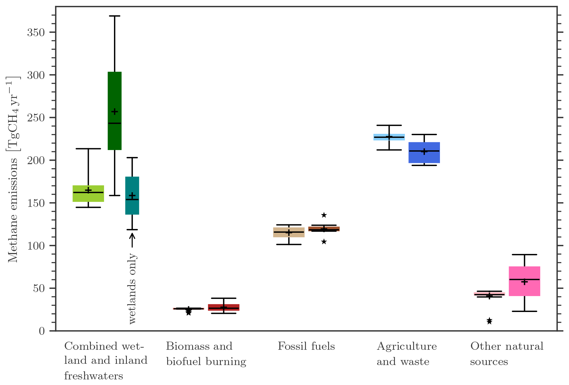
Figure 6Methane global emissions from five broad categories (see Sect. 2.3) for the 2010–2019 decade for top-down inversion models (left light-coloured boxplots) (in Tg CH4 yr−1) and for bottom-up models and inventories (right dark-coloured boxplots). For combined wetland and inland freshwaters three estimates are given: top-down estimates (left), bottom-up estimates (middle), and bottom-up estimates (right) for wetlands only. Median value and first and third quartiles are presented in the boxes. The whiskers represent the minimum and maximum values when suspected outliers are removed (see Sect. 2.2). Suspected outliers are marked by stars. Bottom-up quartiles are not available for bottom-up estimates, except for wetland emissions. Mean values are represented by “+” symbols; these are the values reported in Table 3.
5.1.2 Global methane emissions per source category
The global CH4 emissions from natural and anthropogenic sources (see Sect. 2.3) for 2010–2019 are presented in Figs. 6 and 7 and Table 3. Top-down estimates attribute about 65 % of total emissions to anthropogenic activities (range of 55 %–70 %) and 35 % to natural emissions. Bottom-up estimates attribute 57 % of emissions to direct anthropogenic and the rest to natural plus indirect anthropogenic emissions. A current predominant role of direct anthropogenic sources of CH4 emissions is consistent with and strongly supported by available ice core and atmospheric CH4 records. These data indicate that atmospheric CH4 varied around 700 ppb during the last millennium before increasing by a factor of 2.6 to ∼ 1800 ppb since pre-industrial times. Accounting for the decrease in mean lifetime over the industrial period, Prather et al. (2012) estimated from these data a total source of 554 ± 56 Tg CH4 in 2010, of which about 64 % (352 ± 45 Tg CH4) was of direct anthropogenic origin, consistent with the range in our top-down estimates.
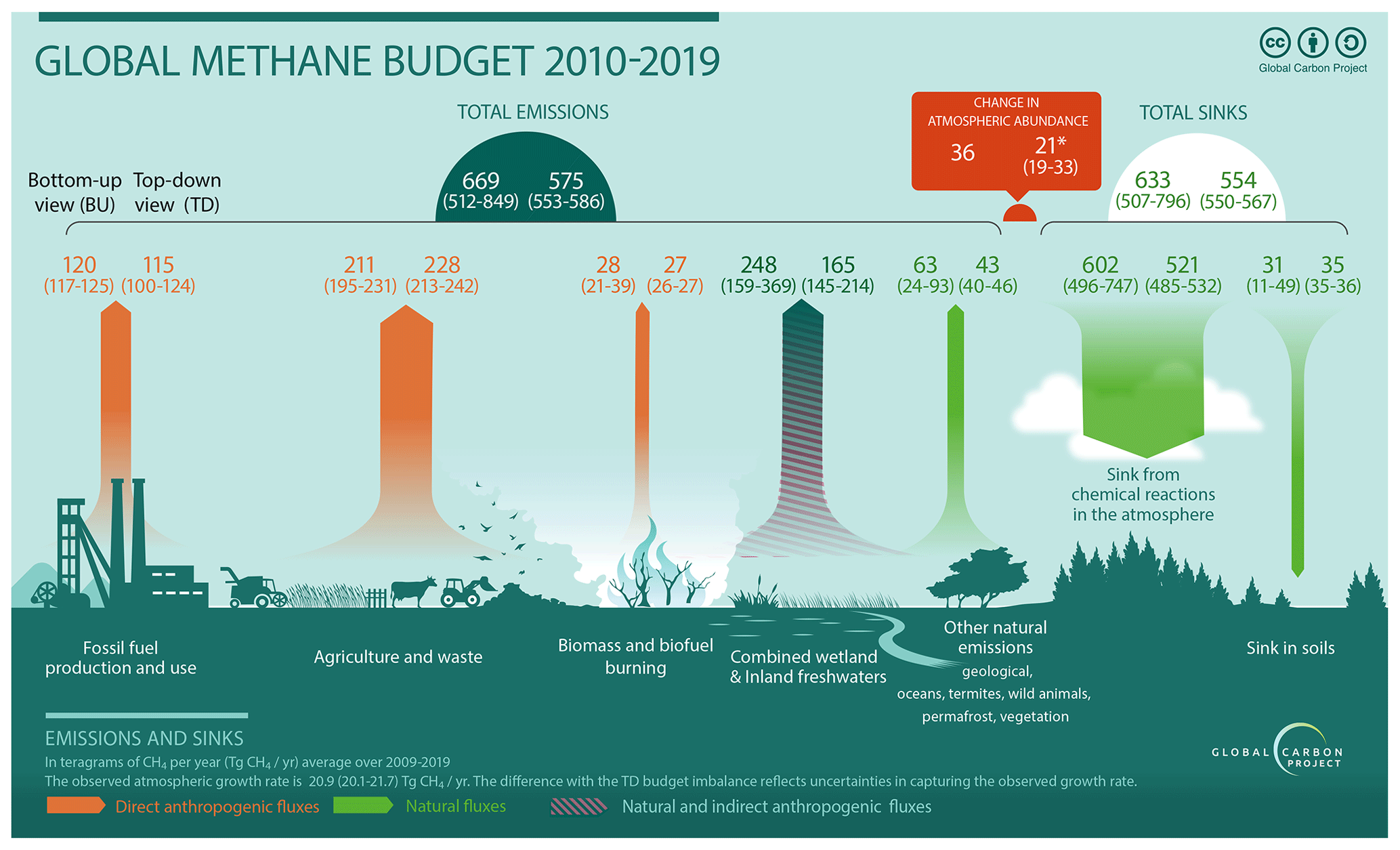
Figure 7The Global Methane Budget for the 2010–2019 decade. Both bottom-up (left) and top-down (right) estimates are provided for each emission and sink category (in Tg CH4 yr−1), as well as for total emissions and total sinks. Combined wetland and inland freshwaters are depicted as natural and indirect anthropogenic sources (darker green and pink hatches) to recall Fig. 4 (Sect. 3.2.2). Adapted from Saunois et al. (2016, 2020).
Natural and indirect anthropogenic emissions
Although smaller than in previous Global Methane Budget releases, the main remaining discrepancy between top-down and bottom-up budgets is found for the natural and indirect anthropogenic emission total (105 Tg), with 311 [183–462] Tg CH4 yr−1 for bottom-up and only 206 [188–225] Tg CH4 yr−1 for top-down over the 2010–2019 decade (Table 3). In the bottom-up estimates, this discrepancy comes first from the estimates in both inland freshwater sources (64 Tg) and second from other natural sources (20 Tg from geological sources, termites, oceans, and permafrost). The top-down approaches may be biased due to missing fluxes (mainly inland freshwaters) in their prior estimates.
For 2010–2019, the top-down and bottom-up derived estimates for wetlands emissions of 165 [145–214] Tg CH4 yr−1 and 159 [119–203] Tg CH4 yr−1 (Table 3) respectively are comparable within their range. Based on diagnostic wetland area values (see notes in Table 3), bottom-up mean wetland emissions for the 2000–2009 period are smaller in this study than those of Saunois et al. (2016) but larger than in Saunois et al. (2020). The changes in wetland emissions from bottom-up models may be related to updates on the wetland extent data set (WAD2M), the use of two different meteorological forcings for this study, and a different set of models (see Sect. 3.2.1). Conversely, the current 2000–2009 mean top-down wetland estimates are lower than those of Saunois et al. (2016) and Saunois et al. (2020) (Table 3). In the bottom-up estimates, the amplitude of the range of emissions of 116–189 is roughly similar to Saunois et al. (2016) (151–222) and Saunois et al. (2020) (102–179) for 2000–2009. Here, the larger range in bottom-up estimates of wetland emissions is due to the use of GSWP3-W5E5 and greater sensibilities of some models to the climate parameters, as discussed in Sect. 3.2.1. Bottom-up and top-down estimates for wetland emissions agree better in this study (∼ 5 Tg yr−1 for 2000–2009) than in Saunois et al. (2016, 2020) (∼ 17 Tg yr−1 and ∼ 30 Tg yr−1 respectively). Natural emissions from inland freshwater systems were not included in the prior fluxes used in the top-down approaches, due to unavailable or uncertain gridded products at the start of the modelling activity. However, emissions from these inland freshwater systems may be implicitly included in the posterior estimates of the top-down models, as these two sources are close and probably overlap at the rather coarse resolution of the top-down models. This is the reason why the “wetland emissions” in the top-down budget in fact better correspond to the sum of combined wetland and inland freshwater emissions in the bottom-up budget. The double counting of 23 Tg CH4 reduces the bottom-up budget for combined wetland and inland freshwaters from 271 Tg CH4 yr−1 to 248 Tg CH4 yr−1 (Sect. 3.2.2). Comparing the 2000–2009 decadal emissions from wetlands and inland freshwater ecosystems estimated by the bottom-up approaches across the last three Global Methane Budget articles shows an upward and then a downward revision with 305 (183 + 122) Tg CH4 yr−1, 356 (147 + 209) Tg CH4 yr−1, and 248 (159 + 112 − 23) Tg CH4 yr−1 (respectively from Saunois et al. (2016, 2020) and this work; the sum in brackets corresponds to the sum of vegetated wetland emissions and inland water emissions estimated through the different budgets). The combined wetland and inland freshwater emissions discrepancy between bottom-up and top-down approaches amounts to 105 Tg CH4 yr−1 for the 2010–2019 decade. From a top-down point of view, the sum of all the natural sources is more robust than the partitioning between wetlands, inland waters, and other natural sources. Including all known spatiotemporal distributions of natural emissions in top-down prior fluxes would be a step forward in consistently comparing natural versus anthropogenic total emissions between top-down and bottom-up approaches.
In the top-down budget, wetlands represent 28 % on average of the total methane emissions but only 24 % in the bottom-up budget (because of higher total emissions inferred) (see Table 3). Given the large uncertainties, neither bottom-up nor top-down approaches included in this study point to significant changes in wetland emissions between the two decades 2000–2009 and 2010–2019 at the global scale.
For the 2010–2019 decade, top-down inversions infer “other natural emissions” (Table 3) at 43 [40–46] Tg CH4 yr−1, whereas the sum of the individual bottom-up emissions is 63 [24–93] Tg CH4 yr−1, contributing to a 20 Tg discrepancy between bottom-up and top-down approaches. Atmospheric inversions infer the same amount over the decade 2000–2009 as over 2010–2019, which is almost half of the value reported in Saunois et al. (2016) (68 [21–130] Tg CH4 yr−1). This reduction in magnitude and uncertainty is due to (1) a more consistent way of considering other natural emissions in the various inverse systems (same prior estimate as in this budget) and (2) a difference in the ensemble of top-down inversions reported here compared to previous releases. It is worth noting that most of the top-down models include about the same ocean and onshore geological emissions and termite emissions in their prior scenarios. However, none include freshwater or permafrost emissions in their prior fluxes and thus in their posterior estimates.
Geological emissions are associated with relatively large uncertainties, and marine seepage emissions are still widely debated (Thornton et al., 2020). However, summing up all bottom-up fossil-CH4-related sources (including anthropogenic emissions) leads to a total of 165 [135–190] Tg CH4 yr−1 in 2010–2019, which is about 29 % of the top-down global CH4 emissions and 25 % of the bottom-up total global estimate. These results agree with the value inferred from 14C atmospheric isotopic analyses of 30 % contribution of fossil-CH4 to global emissions (Etiope et al., 2008; Lassey et al., 2007b). These total fossil fuel emissions from bottom-up approaches agree well with the 13C-based estimate of Schwietzke et al. (2016) of 192 ± 32 Tg CH4 yr−1. In the bottom-up budget, the larger total emissions (due to uncertainties in bottom-up estimates of natural emissions) lead to a lower fossil fuel contribution compared to Lassey et al. (2007b).
Direct anthropogenic emissions
Total direct anthropogenic emissions for the period 2010–2019 were assessed to be statistically consistent between top-down (369 Tg CH4 yr−1, range 350–391) and bottom-up approaches (358 Tg CH4 yr−1, range 329–387); however, top-down approaches infer direct anthropogenic emissions larger by 11 Tg CH4 yr−1 on average compared to bottom-up approaches (Table 3). The partitioning of direct anthropogenic emissions between agriculture and waste, fossil fuels extraction and use, and biomass and biofuel burning also shows good consistency between top-down and bottom-up approaches, though top-down approaches still suggest less fossil fuel and more agriculture and waste emissions than bottom-up estimates (Table 3 and Figs. 6 and 7). For 2010–2019, agriculture and waste contributed an estimated 228 [213–242] Tg CH4 yr−1 in the top-down budget and 211 [195–231] Tg CH4 yr−1 in the bottom-up budget. Fossil fuel emissions contributed 115 [100–124] Tg CH4 yr−1 in the top-down budget and 120 [117–125] Tg CH4 yr−1 in the bottom-up budget. Biomass and biofuel burning contributed 27 [26–27] Tg CH4 yr−1 in the top-down budget and 28 [21–39] Tg CH4 yr−1 in the bottom-up budget. Biofuel CH4 emissions rely on very few estimates currently (Wuebbles and Hayhoe, 2002). Although biofuel is a small source globally (∼ 12 Tg CH4 yr−1), more estimates are needed to allow a proper uncertainty assessment. Overall for top-down inversions the global fraction of total emissions for the different source categories is 40 % for agriculture and waste, 20 % for fossil fuels, and 5 % for biomass and biofuel burning. With the exception of biofuel emissions, the uncertainty associated with global anthropogenic emissions appears to be smaller than that of natural sources but with an asymmetric uncertainty distribution (mean significantly different than median). The relative agreement between top-down and bottom-up approaches may indicate a limited capability of the inversion to separate emissions and a dependency to their prior fluxes; this agreement should therefore be treated with caution. Indeed, in poorly observed regions, top-down inversions rely on the prior estimates and bring little or no additional information to constrain (often) spatially overlapping emissions (e.g. in India, China). Also, as many top-down systems solve for the total fluxes at the surface or for some categories that may differ from the GCP categories, their posterior partitioning relies on the prior ratio between categories that are prescribed using bottom-up inventories.
5.1.3 Global budget of total methane sinks
Top-down estimates
The annual CH4 chemical removal from the atmosphere is estimated to be 521 Tg CH4 yr−1 averaged over the period 2010–2019, with an uncertainty of about ±2 % (range 485–532 Tg CH4 yr−1) (Table 3). All the inverse models account for CH4 oxidation by OH and O(1D), and some include stratospheric Cl oxidation (Table S8 to S11). Most of the top-down models use the OH distribution from the TRANSCOM experiment (Patra et al., 2011) either as fixed over the period or including interannual variability from Patra et al. (2021). This study shows no trend in OH and IAV below ±4 %, in agreement with Thompson et al. (2024) (no significant OH trend and IAV < 2 %). As a result, the range of the top-down sink estimates is rather low compared to bottom-up estimates (see below). Differences between transport models affect the chemical removal of CH4, leading to different chemical loss rates, even with the same OH distribution. However, uncertainties in the OH distribution and magnitude (around ±10 % at the global scale; Zhao et al., 2019) are not considered in our study, while they could contribute to a significant change in the chemical sink and then in the derived posterior emissions through the inverse process (Zhao et al., 2020a), around ±17 % at the global scale, much larger than the model spread derived here. The chemical sink represents more than 90 % of the total sink, the rest being attributable to soil uptake (35 [35–36] Tg CH4 yr−1). The rather narrow range is due to the use of the same climatological soil sink provided within the modelling protocol, which is based on Murguia-Flores et al. (2018). This sink estimate used as a prior estimate in the inversions is a bit higher than the mean estimate of the soil sink calculated by bottom-up models (30 Tg CH4 yr−1; Sect. 3.3.4).
Bottom-up estimates
The total chemical loss for the 2010s reported here is 602 Tg CH4 yr−1 with an uncertainty of 21 % (∼ 125 Tg CH4 yr−1). Differences in chemistry schemes in the models (especially in the stratosphere) and in the volatile organic compound treatment probably explain most of the discrepancies among models (Zhao et al., 2019).
5.2 Latitudinal and regional methane budgets
The latitudinal and regional breakdown of the bottom-up budget is based on crude assumptions that we acknowledge here. Natural and indirect anthropogenic emissions are based on wetland gridded products from land surface models and the combination of the maps from lakes and ponds from Johnson et al. (2022b), reservoirs from Johnson (2021), and streams and rivers from Rocher-Ros (2023) and Rocher-Ros (2023), the sum of those three scaled to 89 Tg CH4 yr−1 (shown in Fig. 5) to artificially include the double counting (estimated only at the global scale) and match the global estimate. However, we acknowledge that this procedure distributes the double counting relatively to the final emission distribution and not according to the freshwater ecosystems where the double counting probably occurs. Wild animal and permafrost maps do not exist and are missing from the calculation, leading to at least 3 Tg CH4 yr−1 of discrepancy. However, as mentioned previously (Sect. 3.2.5 and 3.2.7), this 3 Tg CH4 yr−1 estimate is probably underestimated in the bottom-up budget. Geological and ocean sources are based on Etiope et al. (2019) and Weber et al. (2019) gridded products scaled to 50 Tg CH4 yr−1 to be consistent with the reported global values. Finally, we use the termite emission map produced for this budget and used in the global budget. The latitudinal budget does not include the estimates from the FAO and the USEPA for the direct anthropogenic emissions as they are only provided at country scale.
5.2.1 Latitudinal budget of total methane emissions
The latitudinal breakdown of emissions inferred from atmospheric inversions reveals a dominance of emissions in the latitudinal band 90° S–30° N of 364 [337–390] Tg CH4 yr−1, representing 64 % of the global total (Tables 5 and 6). As emissions in the tropics (30° S–30° N) dominate this latitudinal contribution, we may refer to 90° S–30° N as the tropics in the following 32 % of the emissions are from the mid-latitudes (187 [160–204] Tg CH4 yr−1) and 4 % from high latitudes (above 60° N). The amounts of emissions depend on the land surface area of the region; however, the 90° S–30° N latitudinal band represents 53 % of global land surfaces and the boreal region 60–90° N around 13 %. Hence, the relative contribution of the emissions from the 90° S–30° N region is much larger (11 percentage points more) than the percentage of its land surface areas; on the contrary the boreal regions (60–90° N) emissions contribute significantly less than the surface area percentage of this region (9 percentage points less). The ranges around the mean latitudinal emissions are larger than for the global CH4 sources. While the top-down uncertainty is less than ±5 % at the global scale, it increases to ±7 % for the tropics, to ±12 % the northern mid-latitudes, and to more than ± 20 % in the northern high latitudes (for 2010–2019; Table 5). Both top-down and bottom-up approaches consistently show that CH4 decadal emissions have increased by +21–27 Tg CH4 yr−1 in the tropics and by +5–16 Tg CH4 yr−1 in the northern mid-latitudes between 2000–2009 and 2010–2019 using the mean ensemble estimate.
Over 2010–2019, at the global scale, satellite-based inversions infer almost identical emissions to ground-based inversions (difference of +1 [−3 to 9] Tg CH4 yr−1, with GOSAT-based inversion a bit higher than surface measurements-based inversions), when comparing consistently surface versus satellite-based inversions for each system, similar to Saunois et al. (2020). This difference is much lower than the range derived between the different systems (range of 20 Tg CH4 yr−1 using surface- or satellite-based inversions). This result reflects that differences in atmospheric transport among the systems probably have more impact on the estimated global emissions than the types of observations assimilated.
As expected, considering the different coverage of observation data sets, regional distributions of inferred emissions differ depending on the nature of the observations used (satellite or surface). The largest differences (satellite-based minus surface-based inversions) are observed over the tropical region, between −10 and +43 Tg CH4 yr−1 (90° S to 30° N) and the northern mid-latitudes (between −36 and −2 Tg CH4 yr−1). Satellite data provide stronger constraints on fluxes in tropical regions than surface data, due to a much larger spatial coverage. It is therefore not surprising that differences between these two types of observations are found in the tropical band and consequently in the northern mid-latitudes to balance total emissions, thus affecting the north–south gradient of emissions. However, the regional patterns of these differences are not consistent through the different inverse systems. Indeed, some systems found higher emissions in the tropics when using GOSAT instead of surface observations, while others found the opposite. This difference between inversion systems may depend on whether or not a bias correction is applied to the satellite data based on surface observations and also on the modelled horizontal and vertical transports, in the troposphere and in the stratosphere.
5.2.2 Latitudinal methane emissions per source category
The analysis of the latitudinal CH4 budget per source category (Fig. 8 and Table 6) can be performed both for bottom-up and top-down approaches but with limitations. Bottom-up estimates of natural and indirect anthropogenic emissions are based on assumptions as specified at the beginning of this Sect. 5.2. For top-down estimates, as already noted, the partitioning of emissions per source category has to be considered with caution. Indeed, using only atmospheric CH4 observations to constrain CH4 emissions makes this partitioning largely dependent on prior emissions. However, differences in spatial patterns and seasonality of emissions can be utilised to constrain emissions from different categories by atmospheric methane observations (for those inversions solving for different sources categories, see Sect. 2.3).
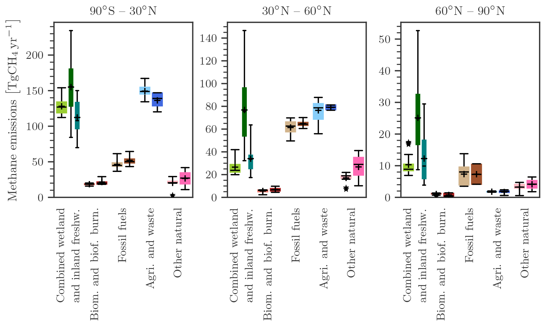
Figure 8Methane latitudinal emissions from five broad categories (see Sect. 2.3) for the 2010–2019 decade for top-down inversion models (left light-coloured boxplots) (in Tg CH4 yr−1) and for bottom-up models and inventories (right dark-coloured boxplots). For combined wetland and inland freshwaters three estimates are given: top-down estimates (left), bottom-up estimates (middle), and bottom-up estimates (right) for wetlands only. Median value and the first and third quartiles are presented in the boxes. The whiskers represent the minimum and maximum values when suspected outliers are removed (see Sect. 2.2). Suspected outliers are marked by stars. Bottom-up quartiles are not available for bottom-up estimates, except wetland emissions. Mean values are represented by “+” symbols; these are the values reported in Table 6.
Agriculture and waste are the largest sources of CH4 emissions in the tropics and the Southern Hemisphere (140 [121–150] Tg CH4 yr−1 in the bottom-up budget and 150 [135–168] Tg CH4 yr−1 in the top-down budget, about 40 % of total CH4 emissions in this region) (Table 6). However, combined wetland and inland freshwater emissions are nearly as large with 151 [85–234] Tg CH4 yr−1 in the bottom-up budget and 128 [112–155] Tg CH4 yr−1 in the top-down budget (Table 6). Anthropogenic emissions dominate in the northern mid-latitudes, with the highest contribution from agriculture and waste emissions (40 % of total emissions in the top-down budget), closely followed by fossil fuel emissions (32 % of total emissions, top-down budget). Boreal regions are largely dominated by inland freshwater emissions (41 % and 54 % of total emissions, top-down and bottom-up budget respectively) (Table 6).
The largest discrepancies between the top-down and the bottom-up budgets are found in the mid-latitudes and boreal regions from the natural and indirect sources with bottom-up estimates twice as large as the top-down ones, especially in the inland freshwater category.
The uncertainty for wetlands and inland freshwater emissions is larger in the bottom-up models than in the top-down models (mostly wetlands), while uncertainty in anthropogenic emissions is larger in the top-down models than in the bottom-up inventories. The large uncertainty in tropical inland freshwater emissions (mostly wetlands) of ±44 % results from large regional differences between the bottom-up land surface models. Although they are using the same forcings, their responses in terms of flux density show different sensitivities to temperature, water vapour pressure, precipitation, and radiation.
5.2.3 Regional budget for total emissions
The regional breakdown of emissions is provided for 18 continental regions (see map in Fig. S3 and Table S1 with the country aggregation in the Supplement).
At the regional scale and for the 2010–2019 decade (Table 7), total methane emissions are dominated by Southeast Asia with 63 [52–71] Tg CH4 yr−1, China with 57 [37–72] Tg CH4 yr−1, and South Asia with 52 [43–60] Tg CH4 yr−1 (top-down budget). These top three emitters contribute 30 % of total global CH4 emissions. The following high-emitting regions are Brazil with 47 [41–58] Tg CH4 yr−1, equatorial Africa with 47 [39–59] Tg CH4 yr−1, the USA with 38 [32–46] Tg CH4 yr−1, southwestern South America with 38 [30–48] Tg CH4 yr−1, Russia with 36 [27–45] Tg CH4 yr−1, Europe with 31 [24–36] Tg CH4 yr−1, the Middle East with 31 [24–39] Tg CH4 yr−1, northern Africa with 25 [23–29] Tg CH4 yr−1, and Canada with 20 [17–24] Tg CH4 yr−1. Other regions contribute less than 20 Tg CH4 yr−1.
Table 7Regional methane emissions (regions ranked by continent) (in Tg CH4 yr−1) for the last decade of 2010–2019, based on top-down and bottom-up approaches. Uncertainties are reported as [min–max] range of reported studies. Differences of 1 Tg CH4 yr−1 in the totals can occur due to rounding errors. For bottom-up approaches, natural and indirect anthropogenic sources are estimated based on available gridded data sets (see text in Sect. 5.2). As some emissions are missing gridded products (wild animals, permafrost, and hydrates), discrepancies may occur in terms of totals proposed in Table 3. Bottom-up direct anthropogenic estimates are based on all products (gridded and per country).
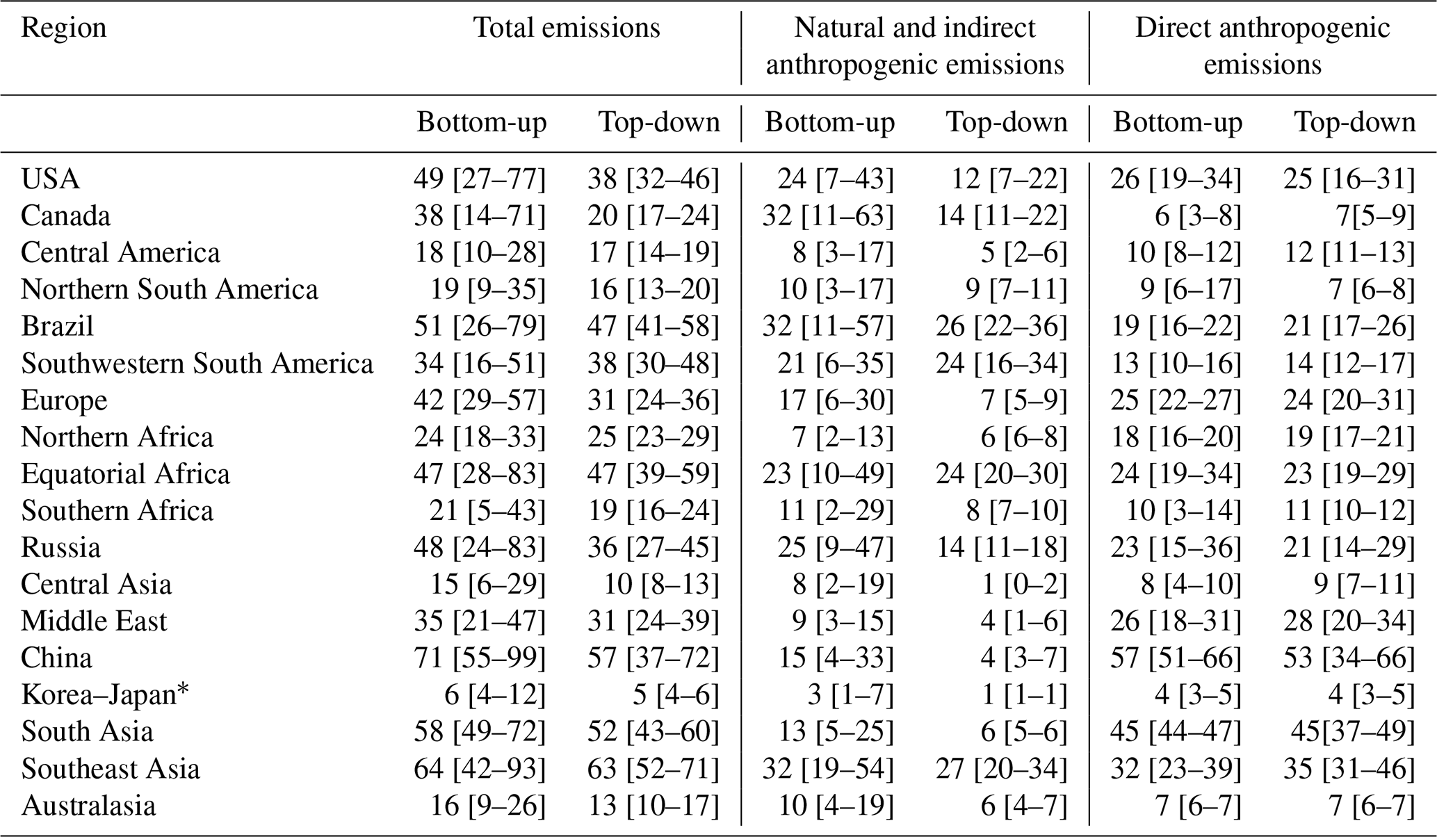
* Korea collectively refers North Korea and South Korea in this table.
5.2.4 Regional budget per source category
In agreement with Stavert et al. (2021), natural and indirect anthropogenic emissions are dominated by Brazil, Canada, Russia, equatorial Africa, and Southeast Asia, contributing 126 Tg CH4 yr−1 in the bottom-up and 105 Tg CH4 yr−1 in the top-down budget (Table 7), i.e. 47 % and 50 % of the global natural and indirect anthropogenic emissions in these budgets respectively. At regional scale also, the ranges of uncertainty in natural and indirect anthropogenic emissions are much larger in the bottom-up budget than in the top-down budget (Fig. S5). Except for four regions (Canada, Brazil, northern South America, southwestern South America), direct anthropogenic emissions contribute more than half of the total regional emissions. Due to the large uncertainty and discrepancies in natural and indirect emissions estimates, the regional direct anthropogenic fractions may differ between the bottom-up and top-down budgets. However, in absolute values, the highest direct anthropogenic emitters are the same in the two budgets, with China and South Asia being the top two by far, contributing 56 [51–66] Tg CH4 yr−1 and 45 [44–47] Tg CH4 yr−1, respectively (bottom-up values; Fig. 9 and Table 7). These two regions contribute 28 % (26 %) of the global direct anthropogenic emissions in the bottom-up (top-down) budget. The ranks of direct anthropogenic emitters are similar to those presented in the last budget (Stavert et al., 2021). Southeast Asia, the USA, the Middle East, Europe, equatorial Africa, and Russia emit between 32 and 23 Tg CH4 yr−1 as direct anthropogenic emissions (bottom-up values; Fig. 8). Brazil, northern Africa, and southwestern South America emit between 10 and 20 CH4 yr−1, while the rest of the regions emit less than 10 CH4 yr−1 direct anthropogenic emissions (Table 7 and Fig. S5).
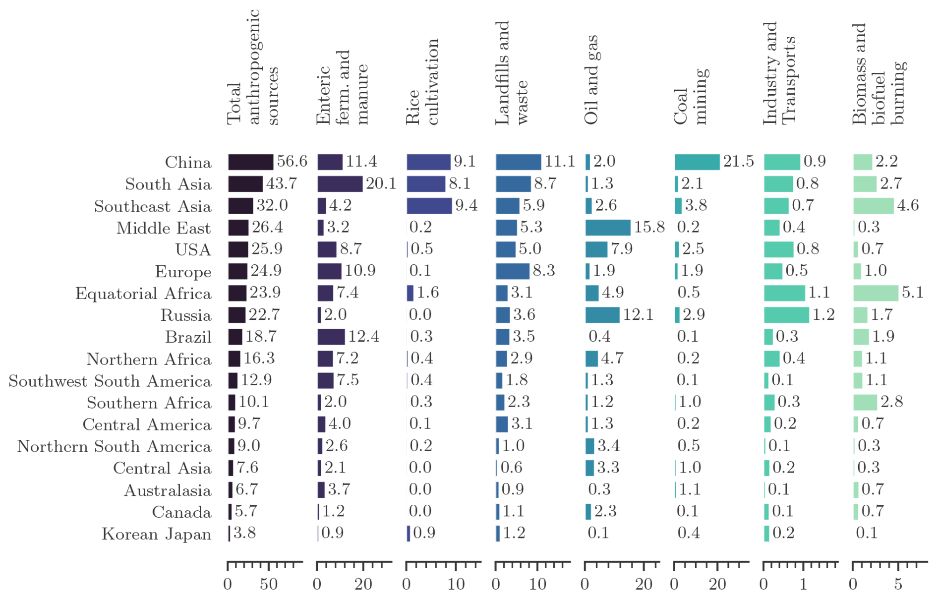
Figure 9Regional anthropogenic emissions for the 2010–2019 decade from bottom-up estimates (in Tg CH4 yr−1). Regions are ranked by their total anthropogenic emissions. Note that each category has its own emission scale. Note that Korea collectively refers to North Korea and South Korea in this figure.
The sectoral partitioning at the regional scale has been derived from both bottom-up and top-down approaches. However, the top-down budget has more limitations, as the sectoral partitioning is usually based on the prior fluxes fractions at the pixel scale, and assimilating only total methane observations does not allow one to disentangle the different source sectors overlapping in a pixel grid. However, differences in spatial patterns and seasonality of emissions can still be constrained by atmospheric CH4 observations for those inversions solving for different sources categories (see Sect. 2.3).
Bottom-up approaches allow deeper sectorial splitting, especially in terms of direct anthropogenic emissions (Fig. 9). Table 7 and Figs. 9 and 10 present the estimations of CH4 emissions on average over 2010–2019. Figure 10 presents the budgets for three main categories (combined wetland and inland freshwaters, fossil fuels, and agriculture and waste); a more detailed figure and table including the five categories is available in the Supplement (Fig. S6 and Tables S13 to S18). Values for each individual data set for the decades 2000–2009, 2010–2019, and the last year 2020 are made available in a spreadsheet (see “Data availability”).
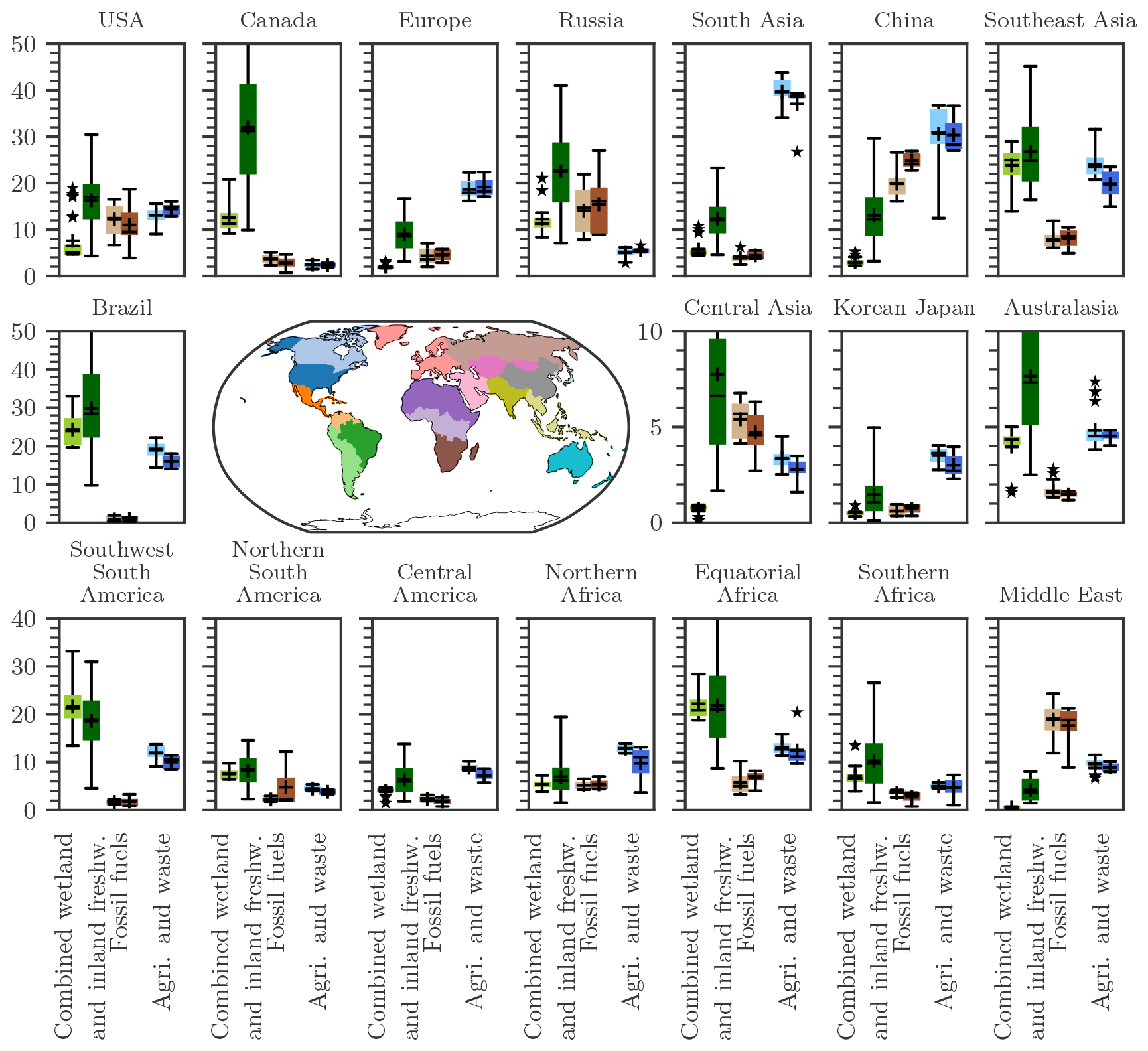
Figure 10Regional emissions (in Tg CH4 yr−1) for three broad main emissions categories for the 2010–2019 decade: combined wetland and inland freshwaters, fossil fuel, and agriculture and waste from top-down estimates (left boxplot) and bottom-up estimates (right boxplots). The inner map shows the region's distribution (also see the Supplement, Table S1 and Fig. S3). More categories are presented in the Supplement in Fig. S6. Note that Korea collectively refers to North Korea and South Korea in this figure.
For most regions, “combined wetland and inland freshwater emissions” are the most uncertain in the bottom-up budget, and generally their range is larger than in the top-down budget. In the top-down budget for 2010–2019 (Table 7), this category contributes the most to the regional emissions in Brazil with24 [20–33] Tg CH4 yr−1, Southeast Asia with 24 [14–29] Tg CH4 yr−1 (though similar to their agriculture and waste emissions of 24 [21–31] Tg CH4 yr−1), equatorial Africa with 22 [19–28] Tg CH4 yr−1, southwestern South America with 22 [14–33] Tg CH4 yr−1, Canada with 12 [9–18] Tg CH4 yr−1, northern South America with 8 [6–10] Tg CH4 yr−1, southern Africa with 7 [4–9] Tg CH4 yr−1. The agriculture and waste emissions category dominates in South Asia with 39 [33–43] Tg CH4 yr−1, China with 30 [13–37] Tg CH4 yr−1, Europe with 19 [16–23] Tg CH4 yr−1, the USA with 13 [9–16] Tg CH4 yr−1, northern Africa with 13 [12–14] Tg CH4 yr−1, Central America with 9 [8–10] Tg CH4 yr−1, and North and South Korea and Japan with 3 [3–4] Tg CH4 yr−1. Fossil fuel emissions dominate in the Middle East with 18 [11–24] Tg CH4 yr−1 and Russia with 14 [8–23] Tg CH4 yr−1 (close to their combined wetland and inland freshwater emissions of 11 [8–13] Tg CH4 yr−1).
The four largest contributors to the fossil fuel sector remain China, the Middle East, Russia, and the USA. Altogether they contribute 67 (64) Tg CH4 yr−1 in the bottom-up (top-down) budget, around 55 % of the global fossil fuel emissions. The bottom-up and top-down approaches generally agree in terms of ensemble mean, except for China for which the top-down estimates suggest lower emissions than the inventories. While Chinese fossil fuel emissions occur mainly through coal mining activity (88 %), the Middle East, Russia, and the USA extract mainly oil and gas (100 %, 80 %, 72 %).
The three largest contributors to the agriculture and waste sector remain South Asia, China, and Southeast Asia. Together they contribute 88 (92) Tg CH4 yr−1 in the bottom-up (top-down) budget, around 40 % of the global agriculture and waste sector (Table 7). While the ensemble means tend to agree between bottom-up and top-down budgets, the uncertainty derived from the top-down approaches is larger, especially for these three regions. CH4 emissions due to rice cultivation originate mostly from these same three regions (Southeast Asia, China, and South Asia). Livestock management emissions occur mainly in South Asia with 20 [18–22] Tg CH4 yr−1, Brazil with 12 [11–13] Tg CH4 yr−1, China with 11 [8–16] Tg CH4 yr−1, and Europe with 11 [10–12] Tg CH4 yr−1 (bottom-up estimates; Table 7). The USA, equatorial Africa, northern Africa, and southwestern South America emit between 7 Tg CH4 yr−1 and 10 Tg CH4 yr−1 in this subsector. Other regions emit less than 4 Tg CH4 yr−1 in the livestock management sector. The waste sector emissions are dominated by three regions: China with 11 [6–14] Tg CH4 yr−1, South Asia with 9 [4–11] Tg CH4 yr−1, and Europe with 8 [6–12] Tg CH4 yr−1 (bottom-up estimates; Table 7). These three regions contribute around 40 % of the global emissions of the waste sector. It is worth noting that the uncertainty in the inventory estimates at the regional scale is around 40 % (from the min–max range of the estimate, not including the uncertainty from each inventory).
The mean emissions estimate for the last year of the budget (2020) was 608 [581–627] Tg CH4 yr−1 (top-down), with 65 % of the emissions from direct anthropogenic sources. This is 65 Tg CH4 yr−1 higher (11 %) than the mean emissions of the 2000–2009 decade and 6 % higher than 2010–2019. In Jackson et al. (2024), we estimated that total methane emissions increased by around 20 % between the early 2000s (2000–2002) and the late 2010s (2018–2020). Year 2020 was the second highest year in terms of atmospheric CH4 growth rate (+15.2 ppb yr−1) since systematic measurements began in the late 1980s, coming in just behind the highest in 2021 at 17.97 ppb yr−1. A few studies analysed the large growth rate increase between 2019 (+9.7 ppb yr−1) and 2020 (+15.2 ppb yr−1) of +5.4 ppb yr−1 (corresponding to +14.4 ± 2.0 Tg CH4 yr−1) (Peng et al., 2022; Stevenson et al., 2022). Peng et al. (2022) estimated that the 2019–2020 growth rate change was almost equally due to an increase in wetland emissions (6.9 ± 2.1 Tg CH4 yr−1) and a decrease in the OH chemical loss (7.5 ± 0.8 Tg CH4 yr−1) due to reduced OH precursor emissions during the COVID lockdown (Laughner et al., 2021). The COVID-19 lockdown resulted in decreased NOx emissions and reduced fossil-fuel-related CH4 emissions (Thorpe et al., 2023), leading to less OH production. At the global scale, Feng et al. (2023) calculated an emission increase of 27 Tg CH4 yr−1 between 2019 and 2020 considering constant OH and a smaller increase of 21 Tg CH4 yr−1 when including a 1.4 % decrease in OH. Increased emissions were mainly found in the northern tropics. Qu et al. (2022) also inferred a 31 Tg CH4 yr−1 increase in emissions, mostly in the tropics, half of it in Africa. Furthermore, Niwa et al. (2024) suggested emission increases by 10–18 Tg CH4 yr−1 in 15° S–10° N and by 20 Tg CH4 yr−1 in 10–35° N from 2016–2019 to 2020–2022. Such a result is compatible with wetland driven abnormal emissions during a consecutive 3-year La Niña event spanning from 2020 to 2022 (Zhang et al., 2023; Nisbet et al., 2023). The difference in terms of methodology and approaches between these three studies makes it difficult to compare them quantitatively but provides a robust understanding on the possible causes. Importantly, all the studies indicate, in various proportions, increasing CH4 emissions in the tropics and in the boreal region, potentially driven by microbial emission from wetlands due to wetter and warmer climate, and a significant contribution of reduced OH concentrations due to the COVID lockdown.
Based on our ensemble of data, we find that top-down approaches infer a much larger change in CH4 emissions (median [Q1–Q3] at +23 [10–31] Tg CH4 yr−1) than bottom-up approaches (−1 [−5 to 3] Tg CH4 yr−1) between 2019 and 2020 (Fig. S7). Bottom-up approaches suggest a very small increase in wetland emissions (around +1 [0–3] Tg CH4 yr−1), while top-down approaches suggest on average a larger increase for wetlands of +8 [5–11] Tg CH4 yr−1, mainly in the tropics and mid-latitudes. It is worth noting that large uncertainties exist for a given year and that the interannual variability is much lower than the ensemble spread. While bottom-up approaches suggest almost constant fossil fuel emissions and slight increase in agriculture and waste (+3 Tg CH4 yr−1), top-down approaches tend to derive higher emissions changes (+6 Tg CH4 yr−1 from the fossil fuel sector and +11 Tg CH4 yr−1 from agriculture and waste as the median over the ensemble). Biomass burning emissions decreased using both approaches by about 5 Tg CH4 yr−1, in agreement with Peng et al. (2022). Some inversions were run with IAV of OH from Patra et al. (2021) and others with constant OH. However, the inferred OH IAVs in 2019 and 2020 are rather low (0.3 % and 0.15 % on yearly average) in Patra et al. (2021), leading to a small impact in terms of emissions changes between 2019–2020, with +22 [9–31] (median [Q1–Q3]) based on the inversions with constant OH and 19 [7–28] based on the inversions with varying OH (Fig. S8).
This first analysis based on our ensemble shows how challenging it is to attribute CH4 emissions changes to a specific sector or region between two years, because related uncertainties remain much larger than the targeted signal to explain. This calls again for further improvement of both approaches.
NOAA estimates 2021 and 2022 methane atmospheric growth rates of 17.8.0 ± 0.5 and 14.0 ± 0.8 ppb yr−1 respectively (Lan et al., 2024). They show a continuation of very high growth rates, challenging again our understanding of the methane budget. The very high values of CH4 growth rate over 2020–2022 have also been accompanied by a sharp decline in the stable isotopic signal, δ13C, which suggests that this recent increase in methane growth rate is at least partly explained by increased emissions from microbial sources such as those found in wetlands, inland waters, agriculture, and waste systems (Nisbet et al., 2023; Michel et al., 2024). However, it is worth noting that almost all aforementioned published top-down studies include constraints only on CH4 and do not discuss the consistency with the atmospheric isotopic signal.
At the time of submission of the manuscript, bottom-up estimates for anthropogenic emissions for 2021 and 2022 were only available from the EDGARv8 data set (https://edgar.jrc.ec.europa.eu/dataset_ghg80, last access: 1 April 2025; EDGAR, 2023). This research inventory suggests that anthropogenic emissions continued to increase from 2020 (374 Tg CH4 yr−1) to 2021 (379 Tg CH4 yr−1) and 2022 (386 Tg CH4 yr−1) with around 62 % of the increase due to the fossil fuel sources, 23 % from the waste sector, and 14 % from the agriculture sector (Table S19). The bottom-up estimate of wetland emissions for 2021–2023, derived from a single wetland model, indicates positive anomalies of 26 Tg CH4 yr−1 in 2020, 23 Tg CH4 yr−1 in 2021, and 21 Tg CH4 yr−1 2022 relative to the 2000–2006 baseline (https://earth.gov/ghgcenter/data-catalog/lpjeosim-wetlandch4-grid-v1, last access: 1 April 2025; Zhang et al., 2023).
In this budget, robust features and uncertainties on sources and sinks estimated by bottom-up or top-down approaches have been highlighted as well as discrepancies between the two budgets. Limitations of the different approaches have also been highlighted. Four shortcomings of the CH4 budget were already identified in Kirschke et al. (2013) and Saunois et al. (2016, 2020) and are revisited below, pointing to key research areas. Although much progress has been made, they are still relevant, and actions are needed. However, these actions fall into different timescales and actors. Here, we revisit the four shortcomings of the contemporary methane budget and discuss how each weakness has been addressed since Saunois et al. (2020). Each section ends by discussing remaining research needs with a list of suggestions, from higher to lower priority.
- 1.
Shortcoming 1. The amount of methane emitted by wetland and inland water systems are still highly uncertain, and double counting may remain.
This first shortcoming has probably received the largest interest in the last few years with significant improvements. First, a community effort has been made based on more studies, documenting or modelling more inland freshwater systems and synthesising emissions from the complex and heterogeneous ensemble of emitting areas: wetlands, ponds, lakes, reservoirs, streams, rivers, estuaries, and marine systems. The range of wetland and inland water emissions has been narrowed down with improved wetland extent and refined estimates for inland freshwater systems. Double counting between inland freshwater systems has been estimated for the first time and accounted for in this budget. All these improvements decreased the discrepancy between top-down and bottom-up estimates of combined wetland and inland freshwater emissions from 156 Tg CH4 yr−1 in Saunois et al. (2020) down to 85 Tg CH4 yr−1 in this update for the 2000–2009 decade. Gridded maps for lakes, ponds, reservoirs, and streams and rivers freshwater emissions have been produced over the past years (Johnson et al., 2021, 2022a; Johnson, 2021; Rocher-Ros et al., 2023; Rocher-Ros, 2023), making the spatial distribution of CH4 sources almost complete for the first time and allowing a better description of prior emissions in future top-down inversions.
Next steps in the short term are listed below from the highest to lowest priority:
- i.
Integration of spatial distribution of inland waters in atmospheric inversion models is needed to reach a full description of prior methane sources and sinks.
- ii.
Refinement is needed of double counting estimation and its possible reduction with more precise spatial and temporal distributions of the different systems contributing to inland freshwater emissions by using very high-resolution satellite data (down to metre resolutions) to properly separate them. The development is needed of a dynamical global high-resolution (typically few metres) classification of saturated soils and inundated surfaces based on satellite data (visible and microwave), surface inventories, and expert knowledge.
- iii.
Ongoing efforts need to be continued to calibrate and evaluate land surface models for wetland emissions against in situ observations such as FLUXNET-CH4 (Knox et al., 2019; Delwiche et al., 2021) or BAWLD-CH4 (Kuhn et al., 2021) for boreal regions and to avoid dependence on top-down estimates. It is still critical to increase the limited number of tropical observations and to assimilate them in the inverse systems to help address the issue (e.g. Kallingal et al., 2024).
- iv.
Ongoing efforts need to be continued to develop a diversity of modelling approaches (among them process-based model or machine learning approaches) to estimate wetland and inland freshwater CH4 emissions, including lateral fluxes and reducing upscaling issues, as done by e.g. Zhuang et al. (2023) for lakes.
- v.
There needs to be continuous integration of collected flux measurements such as in the FLUXNET-CH4 activity (Knox et al., 2019; Delwiche et al., 2021) or in the BAWLD-CH4 data set (Kuhn et al., 2021) to provide global flux maps based on machine learning approaches or other approaches (Peltola et al., 2019; McNicol et al., 2023).
In the long run, developing measurement systems will help to improve estimates of the diversity of wetland and inland freshwater sources and further reduce uncertainties:
-
More systematic measurements of CH4 fluxes and their isotopic signatures from sites reflecting the diversity of environment of wetlands and inland waters, complemented with environmental metadata (e.g. soil temperature and moisture, vegetation types, water temperature, acidity, nutrient concentrations, net primary productivity, soil carbon density for wetlands, lake morphologies) will allow us to better understand and estimate the processes of production and transport to the atmosphere (diffusive, ebullition, plants mediated, etc.) and to better constrain methane fluxes and their isotopic signatures in the different modelling approaches (Glagolev et al., 2011; Turetsky et al., 2014).
- 2.
Shortcoming 2. The uncertainty in the global methane sink from both top-down and bottom-up approaches has not been reduced.
The inverse systems used here have similar caveats to those described in Saunois et al. (2016, 2020) (same OH field, same kind of proxy method to optimise it), leading to quite a constrained atmospheric sink and therefore total global CH4 sources. Although we have used the latest release of CCMI-2022 (Plummer et al., 2021) and CMIP6 simulations (Collins et al., 2017), the uncertainty of derived CH4 chemical loss from the chemistry–climate models remains at the same (large) level compared to the previous intercomparison project ACCMIP (Lamarque et al., 2013). The causes of uncertainties on the CH4 loss and the differences between the different OH fields derived from chemistry–transport models (CTMs) and climate–chemistry models (CCMs) have been widely discussed (e.g. Nicely et al., 2017; Zhao et al., 2019, 2020a). These results emphasise the need to first assess and then improve atmospheric transport and chemistry models, especially vertically, and to integrate robust representation of OH fields in atmospheric models. Recently, numerous efforts based on satellite data have been made to constrain OH distribution, variability, and trends (e.g, Anderson et al., 2023, 2024; Pimlott et al., 2022; Zhao et al., 2023; Zhu et al., 2022). Finally, soil uptake estimates rely on very few studies, and interannual variations remain underconstrained.
Next steps, in the short term, could include developments by the modelling community in the following:
-
The soil uptake needs to be estimated with different land surface models (creating an ensemble), and its variations over the past decade need to be discussed.
-
The impact of using updated and varying soil uptake estimates needs to be assessed, especially considering a warmer climate in the top-down approach. Indeed, for top-down models resolving for the net flux of CH4 at the surface integrating a larger estimate of soil uptake would allow larger emissions and then would reduce the uncertainty with the bottom-up estimates of total CH4 sources.
-
The reactivity of the air parcels in the chemistry–climate models needs to be studied further, and new diagnostics need to be defined to assess modelled CH4 lifetimes such as in Prather et al. (2023).
-
Benchmarking of CTMs and CCMs needs to be developed regarding simulated OH distribution and variability (as in Zhao et al. (2019) for example) to increase efforts to assess biases and improve atmospheric chemical schemes in CTMs and CCMs.
-
Methods need to be developed to better constrain OH. Some have been proposed: satellite CH4 observations (Zhang et al., 2018; Anderson et al., 2023, 2024) could afford this, but strategy is needed (see Duncan et al., 2024, and references therein), and using halogenated compounds beyond methyl chloroform (MCF), such as done in box models (Thompson et al., 2024) to derive a 3D dynamical OH. Such methods should be able to reach very low uncertainty for OH burden and trends (< 2 %) in order to really better constrain the CH4 budget. Duncan et al. (2024) discuss the existing satellite-based methods and propose a strategy to constrain OH from space-based approaches.
-
The aforementioned different potential OH chemical fields need to be integrated, also including interannual variability, to assess the impact on the methane budget following Zhao et al. (2020a).
In the long run, other parameters should be (better) integrated into top-down approaches:
-
The magnitude of the CH4 loss through oxidation by tropospheric Cl is a process debated in the recent literature. More modelling (e.g. Thanwerdas et al., 2022b) and instrumental studies should be devoted to reducing the uncertainty of this potential additional sink before integrating it in top-down models. This would be especially critical if inversions using 13C–CH4 observations were included in GMB in the future.
- 3.
Shortcoming 3. The partitioning of methane sources and sinks by region and emission sectors using top-down approaches are lacking strong constraints.
In this work, we report inversions assimilating satellite data from GOSAT, which bring more constraints than provided by surface stations alone, especially over tropical continents. However, we still found that satellite- and surface-based inversions and the different inversion systems do not consistently infer the same regional flux distribution.
The estimates contributing to the Global Methane Budget are further used in more specific studies focusing on the comparison of the estimates from bottom-up and top-down approaches at national (Deng et al., 2022) and regional scales, including efforts from the GCP-REgional Carbon Cycle Assessment and Processes (RECCAP2) (Petrescu et al., 2021, 2023; Tibrewal et al., 2024; Lauerwald et al., 2023b; and other RECCAP2 publications to come, see https://www.globalcarbonproject.org/reccap/publications.htm, last access: 1 April 2025).
Next steps, in the short term, could integrate developments to be made by the top-down community:
-
GOSAT 2 retrievals should be included (Noël et al., 2022; Imasu et al., 2023) for the GOSAT-based inversions, and TROPOMI-based inversions should be considered (as done in Tsuruta et al., 2023, Shen et al., 2023, Chen et al., 2022, Qu et al., 2021 or Yu et al., 2023) in the next releases once at least 8 years of data are available to provide a decadal estimate and biases are reduced for global-scale use (Lorente et al., 2023; Balasus et al., 2023). Indeed, recent satellite developments have provided higher temporal and spatial resolutions of CH4 observations in regions with poor in situ measurements (Fig. S9; such as TROPOMI observations in northern Africa).
-
Newly available updated gridded products need to be integrated for the different natural sources of CH4 in their prior fluxes (e.g. inland freshwaters) to reach a full spatial description of sources and sinks and to be able to better compare the top-down budget with the bottom-up budget.
-
Newly developed 4D variational inversion systems using isotopic species in the top-down budget need to be integrated (Basu et al., 2022; Thanwerdas et al., 2024; Drinkwater et al., 2023; Mannisenaho et al., 2023).
-
The availability of in situ data at high temporal resolution needs to be improved for the scientific community, especially ones covering poorly documented regions such as China (Liu et al., 2021b; Guo et al., 2020), India (Nomura et al., 2021; Lin et al., 2015; Tiwari and Kumar, 2012), and Siberia (Sasakawa et al., 2010, 2017; Fujita et al., 2020; Winderlich et al., 2010), which have not been delivered so far to international databases or only at poor temporal resolution.
-
Information from imagery satellites needs to be integrated (e.g. TROPOMI, Carbon Mapper, MethaneSAT, GHGSAT) for high to super-emitters to improve prior fluxes of anthropogenic emissions in terms of quantity and locations for each covered sector.
In the long run, integrating more measurements and regional studies will help to improve the top-down systems and further reduce the uncertainties:
-
CH4 surface networks need to be extended to poorly observed regions (e.g. tropics, China, India, high latitudes) and to the vertical dimension. Aircraft regular measurements (e.g. Filges et al., 2015; Brenninkmeijer et al., 2007; Paris et al., 2010; Sweeney et al., 2015), AirCore campaigns (e.g. Andersen et al., 2018; Membrive et al., 2017), and TCCON observations (e.g. Wunch et al., 2011, 2019) remain critical in complementing satellite data that do not observe well in cloudy regions and at high latitudes. Those observations are also crucial to evaluate and eventually correct satellite biases (Buchwitz et al., 2022).
-
Continuous isotopic measurements of CH4 need to be extended and developed to help partitioning methane sources and to be integrated in 4D variational isotopic inversions (e.g. Yacovitch et al., 2021).
-
Global data from future satellite instruments with intrinsic low biases need to be integrated, such as active lidar techniques with MERLIN (Ehret et al., 2017), which are promising to overcome issues of systematic errors (Bousquet et al., 2018) and should provide measurements over the Arctic, contrary to the existing and planned passive missions.
-
Other co-emitted species such as radiocarbon for fossil/non-fossil emissions (Lassey et al., 2007a, 2007b; Petrenko et al., 2017), CO (e.g. Zheng et al., 2019) for biomass burning emissions, and ethane for fugitive emissions (e.g. Ramsden et al., 2022) could bring additional information for partitioning emissions.
- 4.
Shortcoming 4. The atmospheric transport models used in the top-down budget still present issues that have not been fully investigated.
The TRANSCOM experiment synthesised in Patra et al. (2011) showed a large sensitivity of the representation of atmospheric transport on CH4 abundances in the atmosphere. In particular, the modelled CH4 budget appeared to depend strongly on the troposphere–stratosphere exchange rate and thus on the model vertical grid structure and circulation in the lower stratosphere. Also, regional changes in the CH4 budget depend on the characteristics of the atmospheric transport models used in the inversion (Bruhwiler et al., 2017; Locatelli et al., 2015). This axis of research is demanding important development from the atmospheric modelling community. Waiting for future improvements (finer horizontal and vertical resolutions, more accurate physical parameterisation, increase in computing resources, etc.), assessing atmospheric transport error and the impact on the top-down budget remain crucial and mostly rely on the use of an ensemble of models. Methodology changes should be integrated into the next methane budget releases.
Firstly, independent validation should be performed against aircraft measurements (available through the CH4 GLOBALVIEWplus v6.0 ObsPack (Schuldt et al., 2023), the IAGOS data portal (https://iagos.aeris-data.fr/download/, last access: 1 April 2025), the NIES portal (https://db.cger.nies.go.jp/ged/en/datasetlist/index.html, last access: 1 April 2025) for CONTRAIL (e.g.Machida et al., 2008) and Siberian measurements (e.g. Sasakawa et al., 2017), or the WDCGG data portal (https://gaw.kishou.go.jp/, last access: 1 April 2025) for additional flights over three other Japanese airports and Orléans, France). Secondly, AirCore data sets (available through the NOAA Global Monitoring Laboratory website (https://gml.noaa.gov/aftp/data/AirCore/, last access: 1 April 2025, Baier et al., 2021) and the French AirCore programme for atmospheric sampling (https://aircore.aeris-data.fr, last access: 1 April 2025, Membrive et al., 2017)) should be used to evaluate the vertical profile of methane in the models. Then those evaluations against aircraft and AirCore measurements could be used to sort or weight the different estimates in the top-down budget.
Next steps, in the short term, could include some development to be addressed by the top-down community to reduce atmospheric transport errors:
-
Further methodologies need to be developed to extract stratospheric partial column abundances from observations such as TCCON data (Saad et al., 2014; Wang et al., 2014), AirCore (e.g. Andersen et al., 2018; Membrive et al., 2017), or ACE-FTS (De Mazière et al., 2008) or MIPAS (Glatthor et al., 2024) satellite data.
-
SWIR and TIR measurements need to be combined from space to better constrain the tropospheric column, from TROPOMI and IASI, for example in the MethanePlus ESA project (https://methaneplus.eu/#docs, last access: 1 April 2025, Buchwitz et al., 2024) or GOSAT (Kuze et al., 2020).
-
Transport models codes need to be able to be run on graphics processing units (GPUs) to achieve subdegree-resolution global inversions (Chevallier et al., 2023).
In the long run, there need to be developments within the dynamical core of the atmospheric transport models through the implementation of hexagonal–icosaedric grid with finer resolution (Dubos et al., 2015; Niwa et al., 2017, 2022; Lloret et al., 2023), and improvements in the simulated boundary layer dynamics or troposphere–stratosphere exchanges are promising to reduce atmospheric transport errors.
The data presented here are made available in the belief that their dissemination will lead to greater understanding and new scientific insights into the methane budget and changes to it and help to reduce its uncertainties. For research projects, if the data used are essential to the work to be published or if the conclusion or results largely depend on the data, co-authorship should be considered. Full contact details and information on how to cite the data are given in the accompanying database.
The accompanying database includes a NetCDF file defining the regions used, an archive with the maps of prior fluxes used in the top-down activity, an archive with data corresponding to Figs. 3 and 5, and one Excel file organised in the following spreadsheets.
The file Global_Methane_Budget_2000-2020_v1.0.xlsx includes (1) a summary, (2) the methane observed mixing ratio and growth rate from the four global networks (NOAA, AGAGE, CSIRO and UCI), (3) the evolution of global anthropogenic methane emissions (including biomass burning emissions) used to produce Fig. 2, (4) the global and latitudinal budgets over 2000–2009 based on bottom-up approaches, (5) the global and latitudinal budgets over 2000–2009 based on top-down approaches, (6) the global and latitudinal budgets over 2010–2019 based on bottom-up approaches, (7) the global and latitudinal budgets over 2010– 2019 based on top-down approaches, (8) the global and latitudinal budgets for year 2020 based on bottom-up approaches, (9) the global and latitudinal budgets for year 2020 based on top-down approaches, and (10) the list of contributors to contact for further information on specific data.
This database is available from ICOS Carbon Portal (https://doi.org/10.18160/GKQ9-2RHT, Martinez et al., 2024).
We have built an updated global methane budget by using and synthesising a large ensemble of published methods and new results using a consistent, transparent, and traceable approach, including atmospheric observations and inversions (top-down models), process-based models for land surface emissions and atmospheric chemistry, and inventories of anthropogenic emissions (bottom-up models and inventories). For the 2010–2019 decade, global CH4 emissions are 575 Tg CH4 yr−1 (range of 553–586 Tg CH4 yr−1), as estimated by top-down inversions. About 65 % of global emissions are anthropogenic (range of 63 %–68 %). Bottom-up models and inventories suggest larger global emissions (669 Tg CH4 yr−1 [512–849]) mostly because of larger and more uncertain natural emissions from inland freshwater systems, natural wetlands, geological seepage, and likely some unresolved double counting of these sources. It is also likely that some of the individual bottom-up emission estimates are too high, leading to larger global emissions from the bottom-up approach than the atmospheric constraints suggest. However, the important progress in this update is that for the first time, the bottom-up and top-down budgets agree within their uncertainty ranges. This is substantial progress toward defining more accurate global methane emissions.
The latitudinal breakdown inferred from the top-down approach reveals a dominant role of tropical emissions (∼ 64 %) compared to mid-latitudes (∼ 32 %) and high (∼ 4 %) northern latitudes (above 60° N) emissions.
Our results, including an extended set of atmospheric inversions, are compared with the previous budget syntheses of Kirschke et al. (2013) and Saunois et al. (2016, 2020). They show overall good consistency when comparing the same decade (2000–2009) at the global and latitudinal scales. The magnitude and uncertainty of most natural or indirect anthropogenic sources have been revised and updated. In particular, this new budget benefits from large efforts and collaborations from the research community to provide improved estimates of the magnitude and uncertainty of the different freshwater sources and helps reduce the potential double counting at the global scale. Of note, newly available gridded data sets for lakes, ponds, reservoirs, streams, and rivers allow building latitudinal and regional estimates for all these sources for the first time in these estimates. In the next review, we hope to be able to reduce uncertainties in emissions from inland freshwater systems by better quantifying the emission factors of each contributing subsystems (streams, rivers, lakes, ponds) and estimating double counting at regional scale or avoiding double counting by better defining the surface areas of each ecosystem. Another important priority for improvements is the uncertainty on the chemical loss of CH4, which still needs to be better assessed in both the top-down and the bottom-up budgets. Building on the improvement of the points detailed in Sect. 7, our aim is to update this budget synthesis as a living review paper regularly (∼ every 3 or 4 years). Each update will produce a more recent decadal CH4 budget, highlight changes in emissions and trends, and incorporate newly available data and model improvements.
It is still under debate why exactly there has been a sustained increase in atmospheric CH4 (more than +5 ppb yr−1) since 2007 (Nisbet et al., 2019; Nisbet et al., 2023; Turner et al., 2019). Some likely explanations, already introduced by Saunois et al. (2017) and further investigated by Jackson et al. (2020, 2024) and other studies, include, by decreasing order of certainty, the following: (1) a positive contribution from microbial and fossil sources (e.g. Nisbet et al., 2019, 2023; Schwietzke et al., 2016; Jackson et al., 2020), a negative contribution from biomass burning emissions before 2014 (Giglio et al., 2013; Worden et al., 2017); (2) a negligible role of Arctic emission changes (e.g. Nisbet et al., 2019; Saunois et al., 2017); and (3) a tropical dominance of the increasing emissions (e.g. Saunois et al., 2017; Jackson et al., 2020; Wilson et al., 2021; Drinkwater et al., 2023). Although the accelerated atmospheric methane growth rate in 2020 (15.2 ppb yr−1) has found some explanation with the impact of the world pandemic in 2020, the sustained observed growth rates in 2021 (17.8 ppb yr−1) and 2022 (14 ppb yr−1) still challenge our understanding of the global methane cycle. While in Jackson et al. (2020, 2024) the increase in CH4 emissions over the last 2 decades is attributed almost entirely to direct anthropogenic emissions, the uncertainty range from the GMB ensemble is large, and the contribution from natural emissions (wetlands) is still largely uncertain. Besides the decadal change in CH4 emissions, large interannual variability can occur from these natural emissions. The recent high record of CH4 growth rate highlights the potential of large variations from natural emissions from one year to another, in particular wetland emissions (e.g. Peng et al., 2022; Feng et al., 2023). These remain the challenges to be overcome in better quantifying global methane emissions.
Further investigation is needed in follow-up studies to (1) compare these results to the official UNFCCC declarations and to important assessment (as those of IEA) as done previously for example in Deng et al. (2022, 2024) or more specifically for fossil fuel emissions in Tibrewal et al. (2024) and (2) further discuss the trend and interannual variability of CH4 sources and sinks at sectoral and regional scales as in Jackson et al. (2020, 2024), Stavert et al. (2021), or RECCAP2-related publications (e.g. Petrescu et al., 2021, 2023; Lauerwald et al., 2023b; Hugelius et al., 2024) and discuss the compatibility of the budget against the atmospheric isotopic signal such as in Saunois et al. (2017). The next budgets will be critical to assess whether the Global Methane Pledge is successful and assess methane mitigation efforts.
The GCP will continue to support and coordinate the development of improved flux estimates for all budget components and new underlying science to support improved modelling, acquisition of observations, and data integration. At regular intervals (3–4 years), we will continue to bring all flux components together to produce an improved and updated global CH4 budget and provide a global benchmark for other CH4 products and assessments.
Table A1Comparison of terminologies used in this study and previous reports for methane sources.
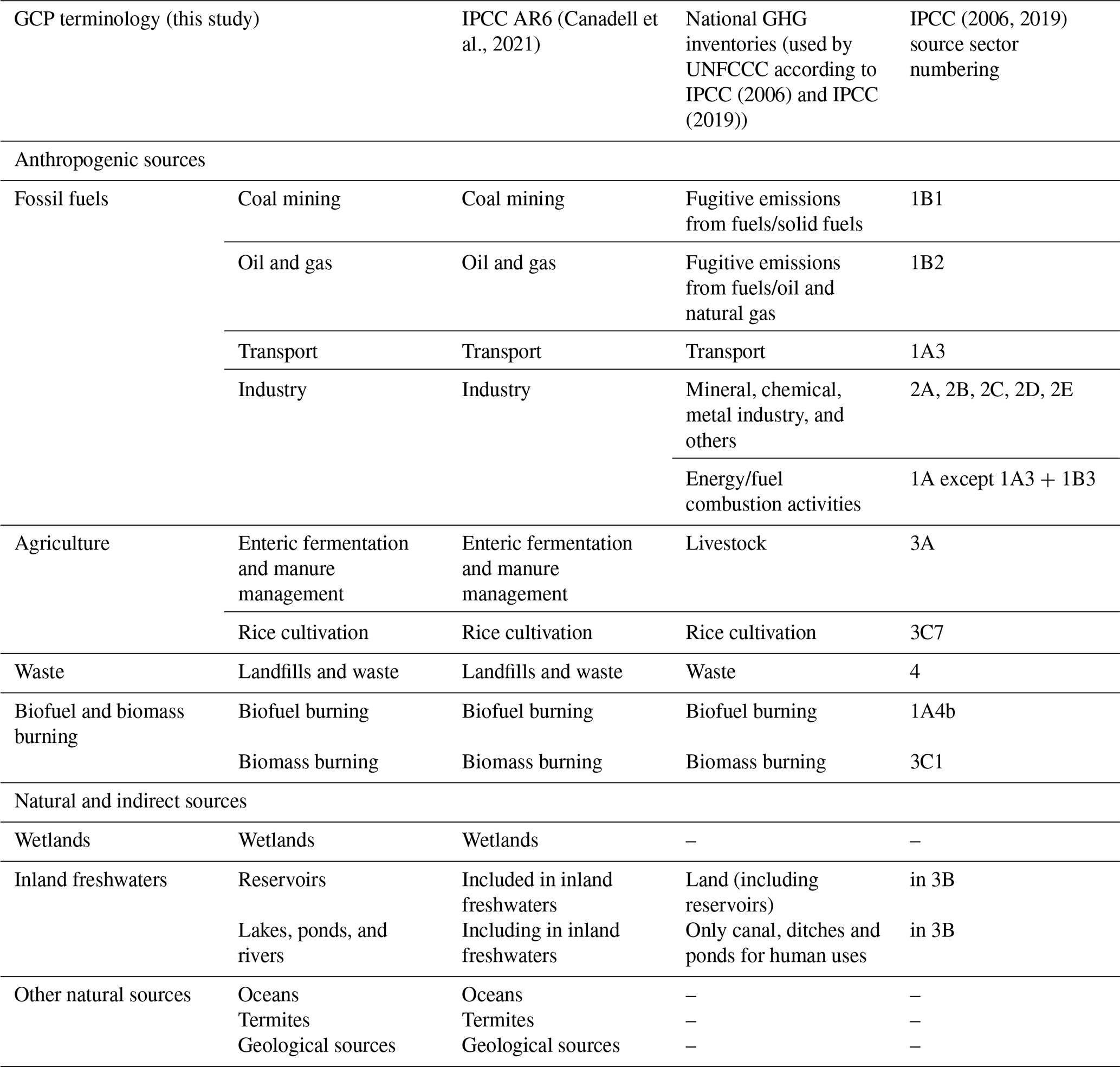
Table A2Summary of methodological changes since the previous budget (Saunois et al., 2020). No significant changes have been applied to the vegetation (Sect. 3.2.8), wild animal (Sect. 3.2.5), and terrestrial permafrost and hydrates (Sect. 3.2.7) estimates, though literature has been expanded and/or updated.
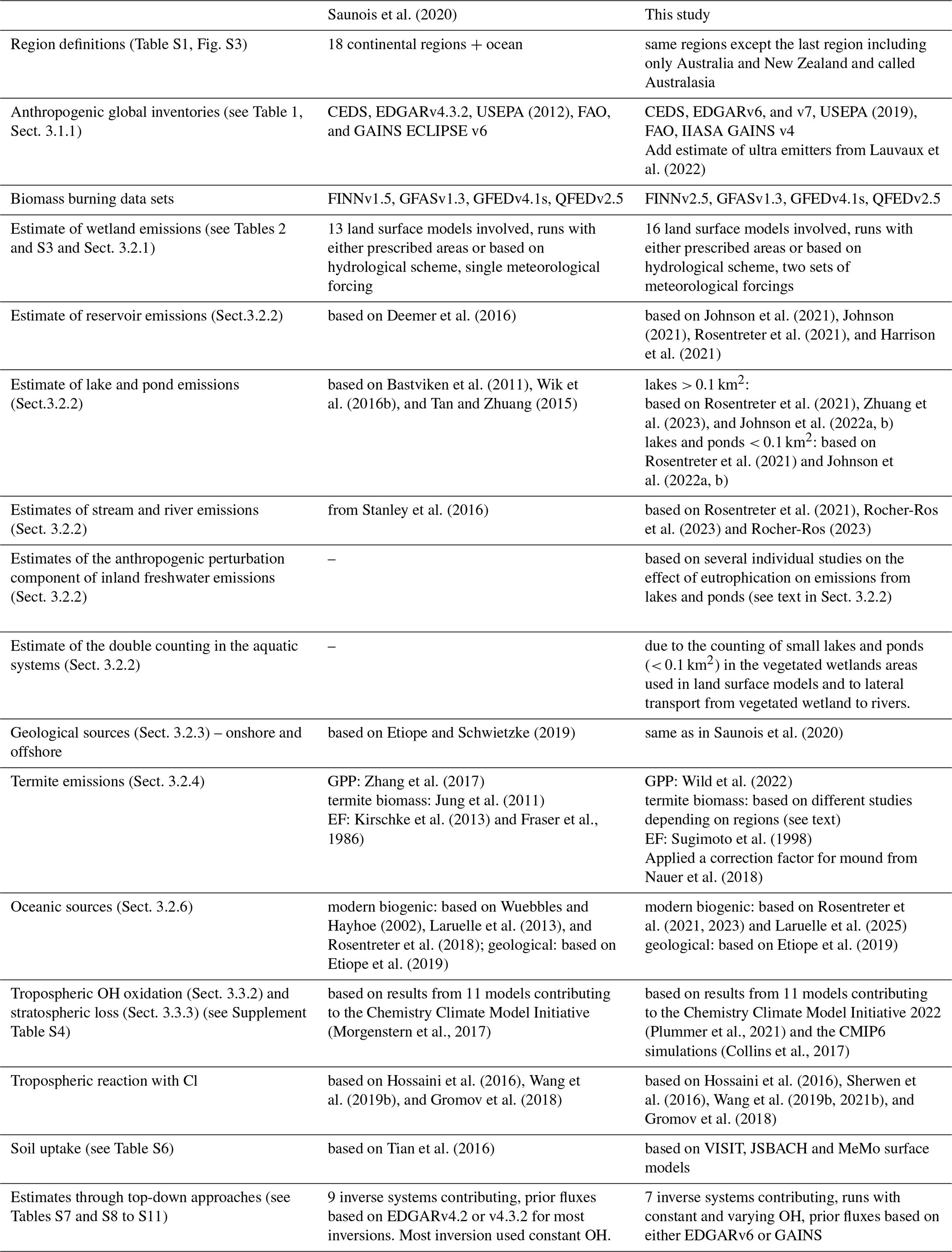
Table A3Funding supporting the production of the various components of the global methane budget in addition to the authors' supporting institutions (see also acknowledgements).
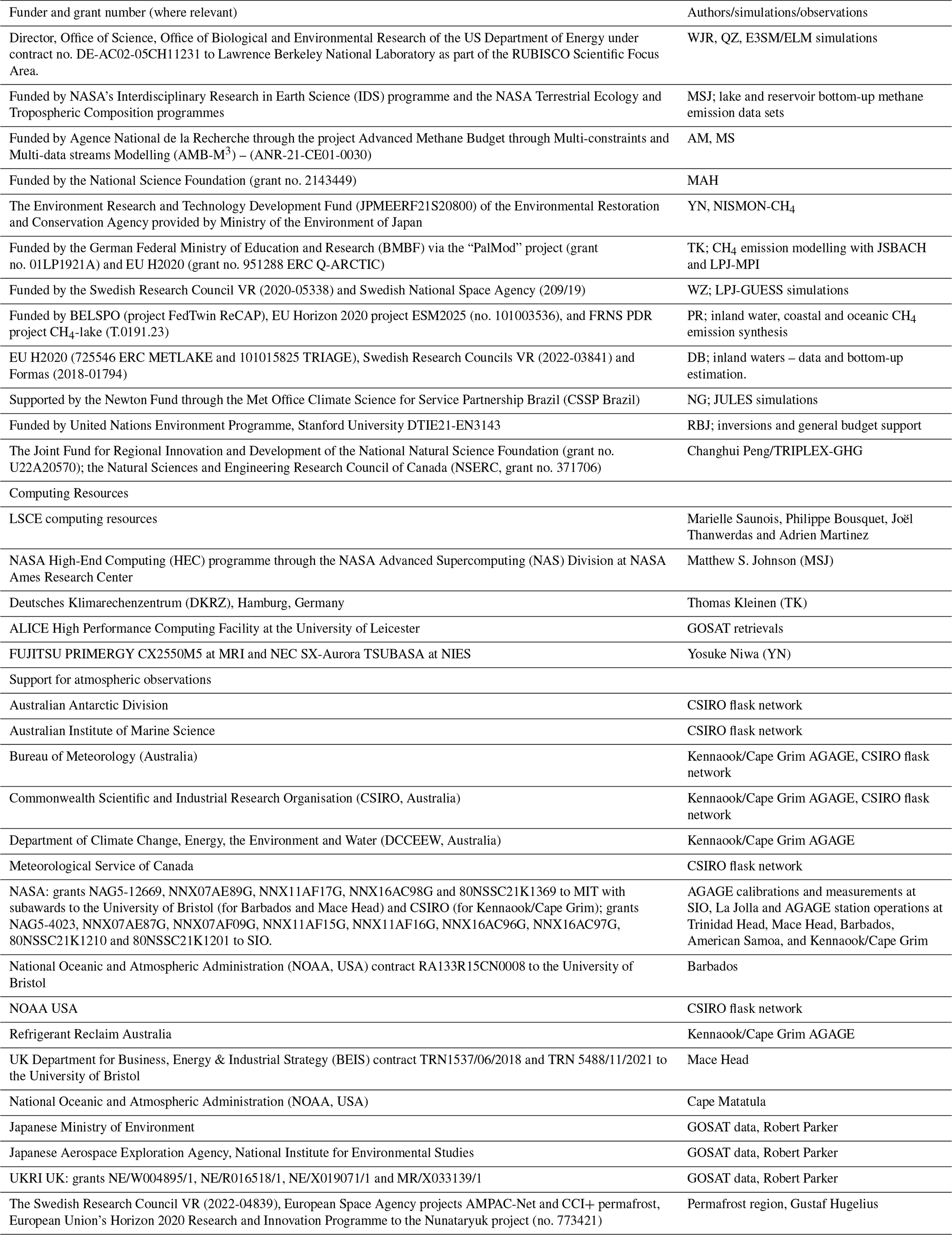
A former version of this article was published on 15 July 2020 and is available at https://doi.org/10.5194/essd-12-1561-2020.
The supplement related to this article is available online at https://doi.org/10.5194/essd-17-1873-2025-supplement.
MS, AM, and JT gathered the bottom-up and top-down data sets and performed the post-processing and analysis.
MS, BP, PB, PeC, and RJ coordinated the global budget. MS, BP, PB, PeC, RJ, PP, and PCi contributed to the update of the full text, and all coauthors appended comments. AM, ED, and XL produced the figures. DJB, NG, PH, AI, AJ, TK, TL, XL, KMcD, JMe, JMu, SP, CP, WR, HT, YY, WZ, ZZ, Qing Z, Qiuan Z, and Qianlai Z performed surface land model simulations to compute wetland emissions. GA, DB, SC, BRD, GE, MAH, GH, MSJ, RL, SN, GRR, JAR, EHS, PRa, PRe, and TSW provided data sets useful for natural emission estimates and/or contributed to text on bottom-up natural emissions. LHI, SJS, TNF, GRvW, and MC provided anthropogenic data sets and contributed to the text for this section. AM, JT, PP, DBe, RJ, YN, AS, AT, and BZ performed atmospheric inversions to compute top-down methane emission estimates for sources and sinks. EJD, XL, DRB, PBK, JM, RJP, MR, MS, DWo, and YYo are PIs of atmospheric observations used in top-down inversions and/or contributed the text describing atmospheric methane observations. FD, MS, and JT contributed to the bottom-up chemical sink section by providing data sets, processing data, and/or contributing to the text. FMF provided data for the soil sink.
At least one of the (co-)authors is a member of the editorial board of Earth System Science Data. The peer-review process was guided by an independent editor, and the authors also have no other competing interests to declare.
Publisher’s note: Copernicus Publications remains neutral with regard to jurisdictional claims made in the text, published maps, institutional affiliations, or any other geographical representation in this paper. While Copernicus Publications makes every effort to include appropriate place names, the final responsibility lies with the authors.
This paper is the result of a collaborative international effort under the umbrella of the Global Carbon Project, a project of Future Earth and a research partner of the World Climate Research Programme (WCRP). We acknowledge all the people and institutions who provided the data used in the global methane budget as well as the institutions funding parts of this effort (see Table A3). We are very grateful for the help provided by Alex Vermeulen in publishing the Global Methane Budget data set on the Integrated Carbon Observation System (ICOS) website. We acknowledge the modelling groups for making their simulations available for this analysis, the joint WCRP Stratosphere-troposphere Processes And their Role in Climate/International Global Atmospheric Chemistry (SPARC/IGAC) Chemistry-Climate Model Initiative (CCMI) for organising and coordinating the model data analysis activity, and the British Atmospheric Data Centre (BADC) for collecting and archiving the CCMI model output. We acknowledge the long-term support provided by the Commonwealth Scientific and Industrial Research Organisation (CSIRO) and the National Environmental Science Program – Climate Systems Hub to coordinate and support activities of the Global Carbon Project. We are grateful to the Emissions Database for Global Atmospheric Research (EDGAR) team (Monica Crippa, Diego Guizzardi, Frederico Pagani, Manjola Banja, Edwin Schaaf, Marilena Muntean, William Becker and Fabio Monforti-Ferrario) for the work needed to publish the EDGAR greenhouse gas emission data sets used in this work (https://edgar.jrc.ec.europa.eu/, last access: 1 April 2025). We are particularly indebted to the dedicated station/instrumental operators/scientists that have gathered the data and ensured their high quality.
More specifically, we acknowledge Adriana Gomez-Sanabria, for her work on waste sector emissions in the GAINS model; Katherine Jensen, for her contribution to the Surface Water Microwave Product Series SWAMPS; Fortunat Joos, for his contribution to simulations with the Land surface Processes and eXchanges model (LPX Bern); Ray Langenfelds and Elise Guerette, for their contribution to the CSIRO network; Paul Miller, for his contribution to simulations with the Lund–Potsdam–Jena General Ecosystem Simulator (LPJ-GUESS); Peng Shushi, for his contribution to simulations with the Organising Carbon and Hydrology In Dynamic Ecosystems (ORCHIDEE) model; Shamil Maksyutov, for his contribution to simulations with the inverse model at the National Institute for Environmental Studies (NIES); Isobel Simpson, for her contribution to the University of California Irvine (UCI) network; Paul Steele, for his former contribution to the CSIRO network; Ray Weiss, for his contribution to the Advanced Global Atmospheric Gases Experiment (AGAGE) network; Christine Widenmeyer, for her contribution to the Fire INventory from the National Center for Atmospheric Research (FINN) database; Xiaoming Xu, for his contribution to simulations with the Integrated Science Assessment Model (ISAM); Yuanzhi Yao, for his contribution to simulations with the Dynamic Land Ecosystem Model (DLEM); Diego Guizzardi, for his contribution to EDGAR; Maria Tenkanen, for her contribution to the Carbon Tracker – Europe (CTE) outputs; and Giulia Conchedda, for her contribution to the Food and Agriculture Organization (FAO) database. FAOSTAT data collection, analysis, and dissemination are funded through FAO regular budget funds. The contribution of relevant experts in member countries is gratefully acknowledged. We acknowledge Juha Hatakka from the Finnish Meteorological Institute (FMI) for making methane measurements at the Pallas station and sharing the data with the community. We thank Ariana Sutton-Grier and Lisamarie Windham-Myers for reviewing an earlier version of the manuscript. Any use of trade, firm, or product names is for descriptive purposes only and does not imply endorsement by the US Government. We warmly thank the three anonymous reviewers for their time and their feedback, which greatly improved the article.
This research has been supported by the Biological and Environmental Research programme (grant no. DE-AC02-05CH11231), the Agence Nationale de la Recherche (grant no. ANR-21-CE01-0030), the Environmental Restoration and Conservation Agency (grant no. JPMEERF21S20800), the Bundesministerium für Bildung und Forschung (grant no. 01LP1921A), Vetenskapsrådet (grant nos. 2020-05338 and 2022-03841), the Swedish National Space Agency (grant no. 209/19), the Belgian Federal Science Policy Office (grant no. FedTwin ReCAP), EU Horizon 2020 (grants nos. 101003536, 951288 ERC Q-ARCTIC, 725546 ERC METLAKE, and 101015825 TRIAGE), the Fonds De La Recherche Scientifique – FNRS (grant no. T.0191.23), the Svenska Forskningsrådet Formas (grant no. 2018-01794), the United Nations Environment Programme (grant no. DTIE21-EN3143), and the Natural Sciences and Engineering Research Council of Canada (grant no. NSERC, no. 371706). Atul K. Jain is supported by the NASA LCLUC programme (award no. 80NSSC24K0920). All funding and support are detailed in Table 3.
This paper was edited by Yuyu Zhou and reviewed by three anonymous referees.
Abe, Y., Bignell, D. E. and Higashi, T. (Eds.): Termites: Evolution, Sociality, Symbioses, Ecology, Springer Netherlands, Dordrecht, https://doi.org/10.1007/978-94-017-3223-9, 2000.
Aho, K. S., Fair, J. H., Hosen, J. D., Kyzivat, E. D., Logozzo, L. A., Rocher-Ros, G., Weber, L. C., Yoon, B., and Raymond, P. A.: Distinct concentration-discharge dynamics in temperate streams and rivers: CO2 exhibits chemostasis while CH4 exhibits source limitation due to temperature control, Limnol. Oceanogr., 66, 3656–3668, 2021.
Allan, W., Lowe, D. C., Gomez, A. J., Struthers, H., and Brailsford, G. W.: Interannual variation of 13C in tropospheric methane: Implications for a possible atomic chlorine sink in the marine boundary layer, J. Geophys. Res.-Atmos., 110, D11360, https://doi.org/10.1029/2004JD005650, 2005.
Allan, W., Struthers, H., and Lowe, D. C.: Methane carbon isotope effects caused by atomic chlorine in the marine boundary layer: Global model results compared with Southern Hemisphere measurements, J. Geophys. Res.-Atmos., 112, D04306, https://doi.org/10.1029/2006jd007369, 2007.
Allen, G. H. and Pavelsky, T. M.: Global extent of rivers and streams, Science, 361, 585–588, https://doi.org/10.1126/science.aat0636, 2018.
Andersen, T., Scheeren, B., Peters, W., and Chen, H.: A UAV-based active AirCore system for measurements of greenhouse gases, Atmos. Meas. Tech., 11, 2683–2699, https://doi.org/10.5194/amt-11-2683-2018, 2018.
Anderson, D. C., Duncan, B. N., Fiore, A. M., Baublitz, C. B., Follette-Cook, M. B., Nicely, J. M., and Wolfe, G. M.: Spatial and temporal variability in the hydroxyl (OH) radical: understanding the role of large-scale climate features and their influence on OH through its dynamical and photochemical drivers, Atmos. Chem. Phys., 21, 6481–6508, https://doi.org/10.5194/acp-21-6481-2021, 2021.
Anderson, D. C., Duncan, B. N., Nicely, J. M., Liu, J., Strode, S. A., and Follette-Cook, M. B.: Technical note: Constraining the hydroxyl (OH) radical in the tropics with satellite observations of its drivers – first steps toward assessing the feasibility of a global observation strategy, Atmos. Chem. Phys., 23, 6319–6338, https://doi.org/10.5194/acp-23-6319-2023, 2023.
Anderson, D. C., Duncan, B. N., Liu, J., Nicely, J. M., Strode, S. A., Follette-Cook, M. B., Souri, A. H., Ziemke, J. R., Gonzales-Abad, G., and Ayazpour, Z.: Trends and interannual variability of the hydroxyl radical in the remote tropics during boreal autumn inferred from satellite proxy data, Geophys. Res. Lett., 51, e2024GL108531, https://doi.org/10.1029/2024GL108531, 2024.
André, J.-C., Boucher, O., Bousquet, P., Chanin, M.-L., Chappellaz, J. and Tardieu, B.: Le méthane: d'où vient-il et quel est son impact sur le climat?, EDP Sciences, Académie des Sciences et Technologies, Paris, ISBN 978-2-7598-1014-7, 2014.
Aoki, S., Nakazawa, T., Murayama, S., and Kawaguchi, S.: Measurements of atmospheric methane at the Japanese Antarctic Station Syowa, Tellus B, 44, 273–281, https://doi.org/10.1034/j.1600-0889.1992.t01-3-00005.x, 1992.
Arora, V. K., Melton, J. R., and Plummer, D.: An assessment of natural methane fluxes simulated by the CLASS-CTEM model, Biogeosciences, 15, 4683–4709, https://doi.org/10.5194/bg-15-4683-2018, 2018.
Bader, W., Bovy, B., Conway, S., Strong, K., Smale, D., Turner, A. J., Blumenstock, T., Boone, C., Collaud Coen, M., Coulon, A., Garcia, O., Griffith, D. W. T., Hase, F., Hausmann, P., Jones, N., Krummel, P., Murata, I., Morino, I., Nakajima, H., O'Doherty, S., Paton-Walsh, C., Robinson, J., Sandrin, R., Schneider, M., Servais, C., Sussmann, R., and Mahieu, E.: The recent increase of atmospheric methane from 10 years of ground-based NDACC FTIR observations since 2005, Atmos. Chem. Phys., 17, 2255–2277, https://doi.org/10.5194/acp-17-2255-2017, 2017.
Baier, B., Sweeney, C., Newberger, T., Higgs, J., Wolter, S., and NOAA Global Monitoring Laboratory: NOAA AirCore atmospheric sampling system profiles (Version 20230831), NOAA GML [data set], https://doi.org/10.15138/6AV0-MY81, 2021.
Balasus, N., Jacob, D. J., Lorente, A., Maasakkers, J. D., Parker, R. J., Boesch, H., Chen, Z., Kelp, M. M., Nesser, H., and Varon, D. J.: A blended TROPOMI+GOSAT satellite data product for atmospheric methane using machine learning to correct retrieval biases, Atmos. Meas. Tech., 16, 3787–3807, https://doi.org/10.5194/amt-16-3787-2023, 2023.
Bansal, S., Van Der Berg, M. P., Fern, R. R., Jones, J. W., Lo, R., McKenna, O. P., Tangen, B. A., Zhang, Z., and Gleason, R. A.: Large increases in methane emissions expected from North America's largest wetland complex, Sci. Adv., 9, eade1112, https://doi.org/10.1126/sciadv.ade1112, 2023.
Barba, J., Bradford, M. A., Brewer, P. E., Bruhn, D., Covey, K., van Haren, J., Megonigal, J. P., Mikkelsen, T. N., Pangala, S. R., Pihlatie, M., Poulter, B., Rivas-Ubach, A., Schadt, C. W., Terazawa, K., Warner, D. L., Zhang, Z., and Vargas, R.: Methane emissions from tree stems: a new frontier in the global carbon cycle, New Phytol., 222, 18–28, https://doi.org/10.1111/nph.15582, 2019.
Barker, P. A., Allen, G., Gallagher, M., Pitt, J. R., Fisher, R. E., Bannan, T., Nisbet, E. G., Bauguitte, S. J.-B., Pasternak, D., Cliff, S., Schimpf, M. B., Mehra, A., Bower, K. N., Lee, J. D., Coe, H., and Percival, C. J.: Airborne measurements of fire emission factors for African biomass burning sampled during the MOYA campaign, Atmos. Chem. Phys., 20, 15443–15459, https://doi.org/10.5194/acp-20-15443-2020, 2020.
Bastviken, D., Tranvik, L. J., Downing, J. A., Crill, P. M., and Enrich-Prast, A.: Freshwater Methane Emissions Offset the Continental Carbon Sink, Science, 331, 50–50, https://doi.org/10.1126/science.1196808, 2011.
Bastviken, D., Treat, C. C., Pangala, S. R., Gauci, V., Enrich-Prast, A., Karlson, M., Gålfalk, M., Romano, M. B., and Sawakuchi, H. O.: The importance of plants for methane emission at the ecosystem scale, Aqua. Bot., 184, 103596, https://doi.org/10.1016/j.aquabot.2022.103596, 2023.
Basu, S., Lan, X., Dlugokencky, E., Michel, S., Schwietzke, S., Miller, J. B., Bruhwiler, L., Oh, Y., Tans, P. P., Apadula, F., Gatti, L. V., Jordan, A., Necki, J., Sasakawa, M., Morimoto, S., Di Iorio, T., Lee, H., Arduini, J., and Manca, G.: Estimating emissions of methane consistent with atmospheric measurements of methane and δ13C of methane, Atmos. Chem. Phys., 22, 15351–15377, https://doi.org/10.5194/acp-22-15351-2022, 2022.
Beaulieu, J. J., DelSontro, T., and Downing, J. A.: Eutrophication will increase methane emissions from lakes and impoundments during the 21st century, Nat. Commun., 10, 1375, https://doi.org/10.1038/s41467-019-09100-5, 2019.
Beck, H., Zimmermann, N., McVicar, T., Vergopolan, N., Berg, A., and Wood, E. F.: Present and future Köppen-Geiger climate classification maps at 1-km resolution, Sci. Data, 5, 180214, doi.org/10.1038/sdata.2018.214, 2018.
Beerling, D. J. and Woodward, F. I.: Vegetation and the Terrestrial Carbon Cycle: Modelling the First 400 Million Years. Cambridge University Press, Cambridge, ISBN 9780521801966, 2001.
Begum, M. S., Bogard, M. J., Butman, D. E., Chea, E., Kumar, S., Lu, X., Nayna, O. K., Ran, L., Richey, J. E., Tareq, S. M., Xuan, D. T., Yu, R., and Park, J.-H.: Localized Pollution Impacts on Greenhouse Gas Dynamics in Three Anthropogenically Modified Asian River Systems, J. Geophys. Res.-Biogeo., 126, e2020JG006124, https://doi.org/10.1029/2020JG006124, 2021.
Bergamaschi, P., Houweling, S., Segers, A., Krol, M., Frankenberg, C., Scheepmaker, R. A., Dlugokencky, E., Wofsy, S. C., Kort, E. A., Sweeney, C., Schuck, T., Brenninkmeijer, C., Chen, H., Beck, V. and Gerbig, C.: Atmospheric CH4 in the first decade of the 21st century: Inverse modeling analysis using SCIAMACHY satellite retrievals and NOAA surface measurements, J. Geophys. Res.-Atmos., 118, 7350–7369, https://doi.org/10.1002/jgrd.50480, 2013.
Bergamaschi, P., Danila, A. M., Weiss, R., Thompson, R. L., Brunner, D., Levin, I., meijer, Y., Chevallier, F., Janssens-Maenhout, G., Bovensmann, H., Crisp, D., Basu, S., Dlugockencky, E. J., Engelen, R., Gerbig, C., Günther, D., Hammer, S., Henne, S., Houweling, S., Karstens, U., Kort, E. A., Maione, M., Manning, A. J., Miller, J., Montzka, S., Pandey, S., Peters, W., Peylin, P., Pinty, B., Ramonet, M., Reimann, S., Röckmann, T., Schmidt, M., Strogies, M., Sussams, J., Tarasova, O., Van Aardenne, J., Vermeulen, A., and Vogel, F.: Atmospheric monitoring and inverse modelling for verification of greenhouse gas inventories, EUR – Scientific and Technical Research Reports, Publications Office of the European Union, https://ec.europa.eu/jrc/en/publication/eur-scientific-and-technical-research-reports/atmospheric-monitoring-and-inverse-modelling-verification-greenhouse-gas-inventories (last access: 17 March 2020a), 2018.
Best, A. I., Richardson, M. D., Boudreau, B. P., Judd, A. G., Leifer, I., Lyons, A. P., Martens, C. S., Orange, D. L., and Wheeler, S. J.: Shallow Seabed Methane Gas Could Pose Coastal hazard, Eos Trans. AGU, 87, 213–217, https://doi.org/10.1029/2006EO220001, 2006.
Bian, L., Gao, Z., Sun, Y., Ding, M., Tang, J., and Schnell, R. C.: CH4 Monitoring and Background Concentration at Zhongshan Station, Antarctica, Atmos. Clim. Sci., 6, 135–144, https://doi.org/10.4236/acs.2016.61012, 2015.
Bignell, D. E. and Eggleton, P.: Termites in ecosystems, in: Termites: Evolution, Sociality, Symbioses, Ecology, edited by: Abe, T., Higashi, M., and Bignell, D. E., Kluwer, Dordrecht, Netherlands, 363–387, 2000.
Biskaborn, B. K., Smith, S. L., Noetzli, J., Matthes, H., Vieira, G., Streletskiy, D. A., Schoeneich, P., Romanovsky, V. E., Lewkowicz, A. G., Abramov, A., Allard, M., Boike, J., Cable, W. L., Christiansen, H. H., Delaloye, R., Diekmann, B., Drozdov, D., Etzelmüller, B., Grosse, G., Guglielmin, M., Ingeman-Nielsen, T., Isaksen, K., Ishikawa, M., Johansson, M., Johannsson, H., Joo, A., Kaverin, D., Kholodov, A., Konstantinov, P., Kröger, T., Lambiel, C., Lanckman, J.-P., Luo, D., Malkova, G., Meiklejohn, I., Moskalenko, N., Oliva, M., Phillips, M., Ramos, M., Sannel, A. B. K., Sergeev, D., Seybold, C., Skryabin, P., Vasiliev, A., Wu, Q., Yoshikawa, K., Zheleznyak, M., and Lantuit, H.: Permafrost is warming at a global scale, Nat. Commun., 10, 264, https://doi.org/10.1038/s41467-018-08240-4, 2019.
Blake, D. R. and Rowland, F. S.: World-wide increase in tropospheric methane, 1978–1983, J. Atmos. Chem., 4, 43–62, 1986.
Blake, D. R., Mayer, E. W., Tyler, S. C., Makide, Y., Montague, D. C., and Rowland, F. S.: Global Increase in Atmospheric Methane Concentrations between 1978 and 1980, Geophys. Res. Lett., 9, 477–480, 1982.
Bloom, A. A., Lee-Taylor, J., Madronich, S., Messenger, D. J., Palmer, P. I., Reay, D. S., and McLeod, A. R.: Global methane emission estimates from ultraviolet irradiation of terrestrial plant foliage, New Phytol., 187, 714–425, https://doi.org/10.1111/j.1469-8137.2010.03259.x, 2010.
Bohn, T. J., Melton, J. R., Ito, A., Kleinen, T., Spahni, R., Stocker, B. D., Zhang, B., Zhu, X., Schroeder, R., Glagolev, M. V., Maksyutov, S., Brovkin, V., Chen, G., Denisov, S. N., Eliseev, A. V., Gallego-Sala, A., McDonald, K. C., Rawlins, M. A., Riley, W. J., Subin, Z. M., Tian, H., Zhuang, Q., and Kaplan, J. O.: WETCHIMP-WSL: intercomparison of wetland methane emissions models over West Siberia, Biogeosciences, 12, 3321–3349, https://doi.org/10.5194/bg-12-3321-2015, 2015.
Bodmer, P., Vroom, R. J. E., Stepina, T., del Giorgio, P. A., and Kosten, S.: Methane dynamics in vegetated habitats in inland waters: quantification, regulation, and global significance, Front. Water, 5, 1332968, https://doi.org/10.3389/frwa.2023.1332968, 2024.
Borges, A. V. and Abril, G.: Carbon Dioxide and Methane Dynamics in Estuaries, in: Treatise on Estuarine and Coastal Science, vol. 5, Academic Press, Waltham, 119–161, https://doi.org/10.1016/B978-0-12-374711-2.00504-0, 2011.
Borges, A. V., Abril, G., and Bouillon, S.: Carbon dynamics and CO2 and CH4 outgassing in the Mekong delta, Biogeosciences, 15, 1093–1114, https://doi.org/10.5194/bg-15-1093-2018, 2018.
Borges, A. V., Darchambeau, F., Lambert, T., Morana, C., Allen, G. H., Tambwe, E., Toengaho Sembaito, A., Mambo, T., Nlandu Wabakhangazi, J., Descy, J.-P., Teodoru, C. R., and Bouillon, S.: Variations in dissolved greenhouse gases (CO2, CH4, N2O) in the Congo River network overwhelmingly driven by fluvial-wetland connectivity, Biogeosciences, 16, 3801–3834, https://doi.org/10.5194/bg-16-3801-2019, 2019.
Borges, A. V., Deirmendjian, L., Bouillon, S., Okello, W., Lambert, T., Roland, F. A. E., Razanamahandry, V. F., Voarintsoa, N. R. G., Darchambeau, F., Kimirei, I. A., Descy, J.-P., Allen, G. H., and Morana, C.: Greenhouse gas emissions from African lakes are no longer a blind spot, Sci. Adv., 8, eabi8716, https://doi.org/10.1126/sciadv.abi8716, 2022.
Bousquet, P., Pierangelo, C., Bacour, C., Marshall, J., Peylin, P., Ayar, P. V., Ehret, G., Bréon, F.-M., Chevallier, F., Crevoisier, C., Gibert, F., Rairoux, P., Kiemle, C., Armante, R., Bès, C., Cassé, V., Chinaud, J., Chomette, O., Delahaye, T., Edouart, D., Estève, F., Fix, A., Friker, A., Klonecki, A., Wirth, M., Alpers, M., and Millet, B.: Error Budget of the MEthane Remote LIdar missioN and Its Impact on the Uncertainties of the Global Methane Budget, J. Geophys. Res.-Atmos., 123, 11766–11785, https://doi.org/10.1029/2018JD028907, 2018.
Brandt, A. R., Heath, G. A., Kort, E. A., O'Sullivan, F., Pétron, G., Jordaan, S. M., Tans, P., Wilcox, J., Gopstein, A. M., Arent, D., Wofsy, S., Brown, N. J., Bradley, R., Stucky, G. D., Eardley, D., and Harriss, R.: Methane Leaks from North American Natural Gas Systems, Science, 343, 733–735, https://doi.org/10.1126/science.1247045, 2014.
Brasseur, G. P. and Solomon, S.: Aeronomy of the Middle Atmosphere: Chemistry and Physics of the Stratosphere and Mesosphere, 3rd Edn., Springer Netherlands, ISBN 978-1-4020-3284-4, 2005.
Brenninkmeijer, C. A. M., Crutzen, P., Boumard, F., Dauer, T., Dix, B., Ebinghaus, R., Filippi, D., Fischer, H., Franke, H., Frieβ, U., Heintzenberg, J., Helleis, F., Hermann, M., Kock, H. H., Koeppel, C., Lelieveld, J., Leuenberger, M., Martinsson, B. G., Miemczyk, S., Moret, H. P., Nguyen, H. N., Nyfeler, P., Oram, D., O'Sullivan, D., Penkett, S., Platt, U., Pupek, M., Ramonet, M., Randa, B., Reichelt, M., Rhee, T. S., Rohwer, J., Rosenfeld, K., Scharffe, D., Schlager, H., Schumann, U., Slemr, F., Sprung, D., Stock, P., Thaler, R., Valentino, F., van Velthoven, P., Waibel, A., Wandel, A., Waschitschek, K., Wiedensohler, A., Xueref-Remy, I., Zahn, A., Zech, U., and Ziereis, H.: Civil Aircraft for the regular investigation of the atmosphere based on an instrumented container: The new CARIBIC system, Atmos. Chem. Phys., 7, 4953–4976, https://doi.org/10.5194/acp-7-4953-2007, 2007.
Bruhwiler, L. M., Basu, S., Bergamaschi, P., Bousquet, P., Dlugokencky, E., Houweling, S., Ishizawa, M., Kim, H.-S., Locatelli, R., Maksyutov, S., Montzka, S., Pandey, S., Patra, P. K., Petron, G., Saunois, M., Sweeney, C., Schwietzke, S., Tans, P., and Weatherhead, E. C.: U.S. CH4 emissions from oil and gas production: Have recent large increases been detected?, J. Geophys. Res.-Atmos., 122, 4070–4083, https://doi.org/10.1002/2016JD026157, 2017.
Brune, A.: Symbiotic digestion of lignocellulose in termite guts, Nat. Rev. Microbiol., 12, 168–180, https://doi.org/10.1038/nrmicro3182, 2014.
Buchwitz, M., de Beek, R., Burrows, J. P., Bovensmann, H., Warneke, T., Notholt, J., Meirink, J. F., Goede, A. P. H., Bergamaschi, P., Körner, S., Heimann, M., and Schulz, A.: Atmospheric methane and carbon dioxide from SCIAMACHY satellite data: initial comparison with chemistry and transport models, Atmos. Chem. Phys., 5, 941–962, https://doi.org/10.5194/acp-5-941-2005, 2005a.
Buchwitz, M., de Beek, R., Noël, S., Burrows, J. P., Bovensmann, H., Bremer, H., Bergamaschi, P., Körner, S., and Heimann, M.: Carbon monoxide, methane and carbon dioxide columns retrieved from SCIAMACHY by WFM-DOAS: year 2003 initial data set, Atmos. Chem. Phys., 5, 3313–3329, https://doi.org/10.5194/acp-5-3313-2005, 2005b.
Buchwitz, M., Dils, B., Reuter, M. , Schneising, O, Hilker , M., Preval, S., Boesch, H.,, Borsdorff, T., Landgraf, J., and Kirsan T. C.: Product Validation and Intercomparison Report (PVIR) version 3 for the Essential Climate Variable (ECV) Greenhouse Gases (GHG), ESA Climate Change Initiative (CCI), report version 16 February 2022, https://climate.esa.int/media/documents/PVIR_GHG-CCIp_v3_reducedsize.pdf (last access: 7 April 2025), 2022.
Buchwitz, M., Schneising, O., Vanselow, S., Houweling, S., van Peet, J., Siddans, R., Kerridge, B., Ventress, L., Knappett, D., Crevoisier, C., Meilhac, N., Borsdof, T., Lorente, A., and Aben, I.: Final Report of the Methane Plus ESA project, TN-D15/16-CH4PLUS, https://methaneplus.eu/#docs (last access: 13 February 2024), 2024.
Butz, A., Guerlet, S., Hasekamp, O., Schepers, D., Galli, A., Aben, I., Frankenberg, C., Hartmann, J. M., Tran, H., Kuze, A., Keppel-Aleks, G., Toon, G., Wunch, D., Wennberg, P., Deutscher, N., Griffith, D., Macatangay, R., Messerschmidt, J., Notholt, J., and Warneke, T.: Toward accurate CO2 and CH4 observations from GOSAT, Geophys. Res. Lett., 38, L14812, https://doi.org/10.1029/2011gl047888, 2011.
Cai, Z. C., Xing, G., Yan, X., Xu, H., Tsuruta, H., Yagi, K., and Minami, K.: Methane and nitrous oxide emissions from rice paddy fields as affected by nitrous fertilizers and water management, Plant Soil, 196, 7–14, 1997.
Cael, B. B., Biggs, J., and Seekell, D. A.: The size-distribution of earth's lakes and ponds: Limits to power-law behavior, Front. Environ. Sci., 10, https://doi.org/10.3389/fenvs.2022.888735, 2022.
Call, M., Maher, D. T., Santos, I. R., Ruiz-Halpern, S., Mangion, P., Sanders, C. J., Erler, D. V., Oakes, J. M., Rosentreter, J., Murray, R., and Eyre, B. D.: Spatial and temporal variability of carbon dioxide and methane fluxes over semi-diurnal and spring–neap–spring timescales in a mangrove creek, Geochim. Cosmochim. Ac., 150, 211–225, https://doi.org/10.1016/j.gca.2014.11.023, 2015.
Canadell, J. G., Monteiro, P. M. S., Costa, M. H., Cotrim da Cunha, L., Cox, P. M., Eliseev, A. V., Henson, S., Ishii, M., Jaccard, S., Koven, C., Lohila, A., Patra, P. K., Piao, S., Rogelj, J., Syampungani, S., Zaehle, S., and Zickfeld, K.: Global Carbon and other Biogeochemical Cycles and Feedbacks, in: Climate Change 2021: The Physical Science Basis. Contribution of Working Group I to the Sixth Assessment Report of the Intergovernmental Panel on Climate Change, edited by: Masson-Delmotte, V., Zhai, P., Pirani, A., Connors, S. L., Péan, C., Berger, S., Caud, N., Chen, Y., Goldfarb, L., Gomis, M. I., Huang, M., Leitzell, K., Lonnoy, E., Matthews, J. B. R., Maycock, T. K., Waterfield, T., Yelekçi, O., Yu, R., and Zhou, B., Cambridge University Press, Cambridge, United Kingdom and New York, NY, USA, 673–816, https://doi.org/10.1017/9781009157896.007, 2021.
Carlson, K. M., Gerber, J. S., Mueller, N. D., Herrero, M., MacDonald, G. K., Brauman, K. A., Havlik, P., O'Connell, C. S., Johnson, J. A., Saatchi, S., and West, P. C.: Greenhouse gas emissions intensity of global croplands, Nat. Clim. Change, 7, 63–68, https://doi.org/10.1038/nclimate3158, 2017.
Castelán-Ortega, O. A., Carlos Ku-Vera, J., and Estrada-Flores, J. G.: Modeling methane emissions and methane inventories for cattle production systems in Mexico, Atmósfera, 27, 185–191, https://doi.org/10.1016/S0187-6236(14)71109-9, 2014.
Cathles, L., Brown, L., Taam, M., and Hunter, A.: A commentary on “The greenhouse-gas footprint of natural gas in shale formations” by R. W. Howarth, R. Santoro, and Anthony Ingraffea, Climatic Change, 113, 525–535, https://doi.org/10.1007/s10584-011-0333-0, 2012.
Chandra, N., Patra, P. K., Bisht, J. S. H., Ito, A., Umezawa, T., Morimoto, S., Aoki, S., Janssens-Maenhout, G., Fujita, R., Takigawa, M., Watanabe, S., Saitoh, N., and Canadell, J. G.: Emissions from the oil and gas sectors, coal mining and ruminant farming drive methane growth over the past three decades, J. Meteorol. Soc. Jpn., 99, 309–337, https://doi.org/10.2151/jmsj.2021-015, 2021.
Chandra, N., Patra, P. K., Fujita, R., Höglund-Isaksson, L., Umezawa, T., Goto, D., Morimoto, S., Vaughn, B. H., and Röckmann, T.: Methane emissions decreased in fossil fuel exploitation and sustainably increased in microbial source sectors during 1990–2020, Comm. Earth Environ., 5, https://doi.org/10.1038/s43247-024-01286-x, 2024.
Chang, J., Peng, S., Ciais, P., Saunois, M., Dangal, S. R. S., Herrero, M., Havlík, P., Tian, H. and Bousquet, P.: Revisiting enteric methane emissions from domestic ruminants and their δ13C CH4 source signature, Nat. Commun., 10, 1–14, https://doi.org/10.1038/s41467-019-11066-3, 2019.
Chang, J., Peng, S., Yin, Y., Ciais, P., Havlik, P., and Herrero, M.: The key role of production efficiency changes in livestock methane emission mitigation, AGU Adv., 2, e2021AV000391, https://doi.org/10.1029/2021AV000391, 2021.
Chappellaz, J., Bluniert, T., Raynaud, D., Barnola, J. M., Schwander, J., and Stauffert, B.: Synchronous changes in atmospheric CH4 and Greenland climate between 40 and 8 kyr BP, Nature, 366, 443–445, https://doi.org/10.1038/366443a0, 1993.
Chen, H., Zhu, Q., Peng, C., Wu, N., Wang, Y., Fang, X., Jiang, H., Xiang, W., Chang, J., Deng, X., and Yu, G.: Methane emissions from rice paddies natural wetlands, lakes in China: Synthesis new estimate, Glob. Change Biol., 19, 19–32, https://doi.org/10.1111/gcb.12034, 2013.
Chen, Y., Hall, J., van Wees, D., Andela, N., Hantson, S., Giglio, L., van der Werf, G. R., Morton, D. C., and Randerson, J. T.: Multi-decadal trends and variability in burned area from the fifth version of the Global Fire Emissions Database (GFED5), Earth Syst. Sci. Data, 15, 5227–5259, https://doi.org/10.5194/essd-15-5227-2023, 2023.
Chen, Y. H. and Prinn, R. G.: Estimation of atmospheric methane emissions between 1996 and 2001 using a three-dimensional global chemical transport model, J. Geophys. Res.-Atmos., 111, D10307, https://doi.org/10.1029/2005JD006058, 2006.
Chen, Z., Jacob, D. J., Nesser, H., Sulprizio, M. P., Lorente, A., Varon, D. J., Lu, X., Shen, L., Qu, Z., Penn, E., and Yu, X.: Methane emissions from China: a high-resolution inversion of TROPOMI satellite observations, Atmos. Chem. Phys., 22, 10809–10826, https://doi.org/10.5194/acp-22-10809-2022, 2022.
Chevallier, F., Lloret, Z., Cozic, A., Takache, S., and Remaud, M.: Toward high-resolution global atmospheric inverse modeling using graphics accelerators, Geophys. Res. Lett., 50, 1–9, https://doi.org/10.1029/2022GL102135, 2023.
Chiri, E., Greening, C., Lappan, R., Waite D. W., Jirapanjawat, T., Dong, X, Arndt, S. K., and Nauer, P. A.: Termite mounds contain soil-derived methanotroph communities kinetically adapted to elevated methane concentrations, ISME J., 14, 2715–273, https://doi.org/10.1038/s41396-020-0722-3, 2020.
Chiri, E., Nauer, P. A., Lappan, R., Jirapanjawat, T., Waite, D. W., Handley, K. M., Hugenholtz, P., Cook, P. L. M., Arndt, S. K., and Greening, C.: Termite gas emissions select for hydrogenotrophic microbial communities in termite mounds, P. Natl. Acad. Sci. USA, 118, e2102625118, https://doi.org/10.1073/pnas.2102625118, 2021.
Ciais, P., Sabine, C., Bala, G., Bopp, L., Brovkin, V., Canadell, J., Chhabra, A., DeFries, R., Galloway, J., Heimann. M, Jones, C., Le Quéré, C., Myneni, R. B., Piao, S., and Thornton, P.: Carbon and Other Biogeochemical Cycles, in In Climate Change 2013: The Physical Science Basis. Contribution of Working Group I to the Fifth Assessment Report of IPCC, edited by: Stocker, T. F., Qin, D., Plattner, G.-K., Tignor, M., Allen, S. K., Boschung, J., Nauels, A., Xia, Y., Bex, V., and Midgley, P. M., Cambridge University Press, Cambridge, ISBN 978-1-107-05799-1, 2013.
Cicerone, R. J. and Oremland, R. S.: Biogeochemical aspects of atmospheric methane, Global Biogeochem. Cy., 2, 299–327, 1988.
Cicerone, R. J. and Shetter, J. D.: Sources of atmospheric methane: Measurements in rice paddies and a discussion, J. Geophys. Res., 86, 7203–7209, 1981.
Collins, W. J., Lamarque, J.-F., Schulz, M., Boucher, O., Eyring, V., Hegglin, M. I., Maycock, A., Myhre, G., Prather, M., Shindell, D., and Smith, S. J.: AerChemMIP: quantifying the effects of chemistry and aerosols in CMIP6, Geosci. Model Dev., 10, 585–607, https://doi.org/10.5194/gmd-10-585-2017, 2017.
Comer-Warner, S. A., Romeijn, P., Gooddy, D. C., Ullah, S., Kettridge, N., Marchant, B., Hannah, D. M., and Krause, S.: Thermal sensitivity of CO2 and CH4 emissions varies with streambed sediment properties, Nat. Commun., 9, 2803, https://doi.org/10.1126/science.aaf2348, 2018.
Conley, S., Franco, G., Faloona, I., Blake, D. R., Peischl, J., and Ryerson, T. B.: Methane emissions from the 2015 Aliso Canyon blowout in Los Angeles, CA, Science, 351, 1317–1320, https://doi.org/10.1126/science.aaf2348, 2016.
Conrad, R., Klose, M., and Claus, P.: Phosphate Inhibits Acetotrophic Methanogenesis on Rice Roots, Appl. Environ. Microbiol., 66(2), 828–831, 2000.
Covey, K. R. and Megonigal, J. P.: Methane production and emissions in trees and forests, New Phytol., 222, 35–51, https://doi.org/10.1111/nph.15624, 2019.
Covey, K. R., Wood, S. A., Warren, R. J., Lee, X., and Bradford, M. A.: Elevated methane concentrations in trees of an upland forest, Geophys. Res. Lett., 39, L15705, https://doi.org/10.1029/2012gl052361, 2012.
Covey, K. R., de Mesquita, C. P. B., Oberle, B., Maynard, D. S., Bettigole, C., Crowther, T. W., Duguid, M. C., Steven, B., Zanne, A. E., Lapin, M., Ashton, M. S., Oliver, C. D., Lee, X., and Bradford, M. A.: Greenhouse trace gases in deadwood, Biogeochemistry, 130, 215–226, https://doi.org/10.1007/s10533-016-0253-1, 2016.
Crawford, J. T. and Stanley, E. H.: Controls on methane concentrations and fluxes in streams draining human-dominated landscapes, Ecol. Appl., 26, 1581–1591, 2016.
Crevoisier, C., Nobileau, D., Fiore, A. M., Armante, R., Chédin, A., and Scott, N. A.: Tropospheric methane in the tropics – first year from IASI hyperspectral infrared observations, Atmos. Chem. Phys., 9, 6337–6350, https://doi.org/10.5194/acp-9-6337-2009, 2009.
Crippa, M., Guizzardi, D., Solazzo, E., Muntean, M., Schaaf, E., Monforti-Ferrario, F., Banja, M., Olivier, J. G. J., Grassi, G., Rossi, S., and Vignati, E.: GHG emissions of all world countries – 2021 Report, EUR 30831 EN, Publications Office of the European Union, Luxembourg, 2021, JRC126363, ISBN 978-92-76-41547-3, https://doi.org/10.2760/173513, 2021.
Crippa, M., Guizzardi, D., Pagani, F., Banja, M., Muntean, M., Schaaf E., Becker, W., Monforti-Ferrario, F., Quadrelli, R., Risquez Martin, A., Taghavi-Moharamli, P., Köykkä, J., Grassi, G., Rossi, S., Brandao De Melo, J., Oom, D., Branco, A., San-Miguel, J., and Vignati, E.: GHG emissions of all world countries, Publications Office of the European Union, Luxembourg, JRC134504, 2023, https://doi.org/10.2760/953322, 2023.
Crutzen, P. J., Aselmann, I., and Seiler, W.: Methane production by domestic animals, wild ruminants, other herbivorous fauna, and humans, Tellus B, 38B, 271–284, https://doi.org/10.1111/j.1600-0889.1986.tb00193.x, 1986.
Cucchi, M., Weedon, G. P., Amici, A., Bellouin, N., Lange, S., Müller Schmied, H., Hersbach, H., and Buontempo, C.: WFDE5: bias-adjusted ERA5 reanalysis data for impact studies, Earth Syst. Sci. Data, 12, 2097–2120, https://doi.org/10.5194/essd-12-2097-2020, 2020.
Cunnold, D. M., Steele, L. P., Fraser, P. J., Simmonds, P. G., Prinn, R. G., Weiss, R. F., Porter, L. W., O'Doherty, S., Langenfelds, R. L., Krummel, P. B., Wang, H. J., Emmons, L., Tie, X. X., and Dlugokencky, E. J.: In situ measurements of atmospheric methane at GAGE/AGAGE sites during 1985-2000 and resulting source inferences, J. Geophys. Res.-Atmos., 107, ACH 20-21–20-18, https://doi.org/10.1029/2001jd001226, 2002.
Curry, C. L.: Modeling the soil consumption of atmospheric methane at the global scale, Global Biogeochem. Cy., 21, GB4012, https://doi.org/10.1029/2006gb002818, 2007.
Darmenov, A. and da Silva, A.: The quick fire emissions dataset (QFED) – Documentation of versions 2.1, 2.2 and 2.4, Technical Report Series on Global Modeling and Data Assimilation, NASA Global Modeling and Assimilation Office, https://gmao.gsfc.nasa.gov/pubs/docs/Darmenov796.pdf (last access: 11 March 2020), 2015.
Deemer, B. R. and Holgerson, M. A.: Drivers of Methane Flux Differ Between Lakes and Reservoirs, Complicating Global Upscaling Efforts, J. Geophys. Res.-Biogeo., 126, e2019JG005600, https://doi.org/10.1029/2019JG005600, 2021.
Deemer, B. R., Harrison, J. A., Li, S., Beaulieu, J. J., DelSontro, T., Barros, N., Bezerra-Neto, J. F., Powers, S. M., dos Santos, M. A., and Vonk, J. A.: Greenhouse Gas Emissions from Reservoir Water Surfaces: A New Global Synthesis, BioScience, 66, 949–964, https://doi.org/10.1093/biosci/biw117, 2016.
Defratyka, S. M., Paris, J.-D., Yver-Kwok, C., Fernandez, J. M., Korben, P., and Bousquet, P.: Mapping Urban Methane Sources in Paris, France, Environ. Sci. Technol., 55, 8583–8591, 10.1021/acs.est.1c00859, 2021.
DelSontro, T., Beaulieu, J. J., and Downing, J. A.: Greenhouse gas emissions from lakes and impoundments: Upscaling in the face of global change, Limnol. Oceanogr. Lett., 3, 64–75, https://doi.org/10.1002/lol2.10073, 2018.
Delwiche, K. B., Knox, S. H., Malhotra, A., Fluet-Chouinard, E., McNicol, G., Feron, S., Ouyang, Z., Papale, D., Trotta, C., Canfora, E., Cheah, Y.-W., Christianson, D., Alberto, Ma. C. R., Alekseychik, P., Aurela, M., Baldocchi, D., Bansal, S., Billesbach, D. P., Bohrer, G., Bracho, R., Buchmann, N., Campbell, D. I., Celis, G., Chen, J., Chen, W., Chu, H., Dalmagro, H. J., Dengel, S., Desai, A. R., Detto, M., Dolman, H., Eichelmann, E., Euskirchen, E., Famulari, D., Fuchs, K., Goeckede, M., Gogo, S., Gondwe, M. J., Goodrich, J. P., Gottschalk, P., Graham, S. L., Heimann, M., Helbig, M., Helfter, C., Hemes, K. S., Hirano, T., Hollinger, D., Hörtnagl, L., Iwata, H., Jacotot, A., Jurasinski, G., Kang, M., Kasak, K., King, J., Klatt, J., Koebsch, F., Krauss, K. W., Lai, D. Y. F., Lohila, A., Mammarella, I., Belelli Marchesini, L., Manca, G., Matthes, J. H., Maximov, T., Merbold, L., Mitra, B., Morin, T. H., Nemitz, E., Nilsson, M. B., Niu, S., Oechel, W. C., Oikawa, P. Y., Ono, K., Peichl, M., Peltola, O., Reba, M. L., Richardson, A. D., Riley, W., Runkle, B. R. K., Ryu, Y., Sachs, T., Sakabe, A., Sanchez, C. R., Schuur, E. A., Schäfer, K. V. R., Sonnentag, O., Sparks, J. P., Stuart-Haëntjens, E., Sturtevant, C., Sullivan, R. C., Szutu, D. J., Thom, J. E., Torn, M. S., Tuittila, E.-S., Turner, J., Ueyama, M., Valach, A. C., Vargas, R., Varlagin, A., Vazquez-Lule, A., Verfaillie, J. G., Vesala, T., Vourlitis, G. L., Ward, E. J., Wille, C., Wohlfahrt, G., Wong, G. X., Zhang, Z., Zona, D., Windham-Myers, L., Poulter, B., and Jackson, R. B.: FLUXNET-CH4: a global, multi-ecosystem dataset and analysis of methane seasonality from freshwater wetlands, Earth Syst. Sci. Data, 13, 3607–3689, https://doi.org/10.5194/essd-13-3607-2021, 2021.
De Mazière, M., Vigouroux, C., Bernath, P. F., Baron, P., Blumenstock, T., Boone, C., Brogniez, C., Catoire, V., Coffey, M., Duchatelet, P., Griffith, D., Hannigan, J., Kasai, Y., Kramer, I., Jones, N., Mahieu, E., Manney, G. L., Piccolo, C., Randall, C., Robert, C., Senten, C., Strong, K., Taylor, J., Tétard, C., Walker, K. A., and Wood, S.: Validation of ACE-FTS v2.2 methane profiles from the upper troposphere to the lower mesosphere, Atmos. Chem. Phys., 8, 2421–2435, https://doi.org/10.5194/acp-8-2421-2008, 2008.
Deng, Z., Ciais, P., Tzompa-Sosa, Z. A., Saunois, M., Qiu, C., Tan, C., Sun, T., Ke, P., Cui, Y., Tanaka, K., Lin, X., Thompson, R. L., Tian, H., Yao, Y., Huang, Y., Lauerwald, R., Jain, A. K., Xu, X., Bastos, A., Sitch, S., Palmer, P. I., Lauvaux, T., d'Aspremont, A., Giron, C., Benoit, A., Poulter, B., Chang, J., Petrescu, A. M. R., Davis, S. J., Liu, Z., Grassi, G., Albergel, C., Tubiello, F. N., Perugini, L., Peters, W., and Chevallier, F.: Comparing national greenhouse gas budgets reported in UNFCCC inventories against atmospheric inversions, Earth Syst. Sci. Data, 14, 1639–1675, https://doi.org/10.5194/essd-14-1639-2022, 2022.
Deng, Z., Ciais, P., Hu, L., Martinez, A., Saunois, M., Thompson, R. L., Tibrewal, K., Peters, W., Byrne, B., Grassi, G., Palmer, P. I., Luijkx, I. T., Liu, Z., Liu, J., Fang, X., Wang, T., Tian, H., Tanaka, K., Bastos, A., Sitch, S., Poulter, B., Albergel, C., Tsuruta, A., Maksyutov, S., Janardanan, R., Niwa, Y., Zheng, B., Thanwerdas, J., Belikov, D., Segers, A., and Chevallier, F.: Global Greenhouse Gas Reconciliation 2022, Earth Syst. Sci. Data Discuss. [preprint], https://doi.org/10.5194/essd-2024-103, in review, 2024.
Denman, K. L., Brasseur, G., Chidthaisong, A., Ciais, P., Cox, P. M., Dickinson, R. E., Hauglustaine, D., Heinze, C., Holland, E., Jacob, D., Lohmann, U., Ramachandran, S., da Silva Dias, P. L., Wofsy, S. C., and Zhang, X.: Couplings Between Changes in the Climate System and Biogeochemistry, in: Climate Change 2007: The Physical Science Basis. Contribution of Working Group I to the Fourth Assessment Report of the Intergovernmental Panel on Climate Change, edited by: Solomon, S., Qin, D., Manning, M., Chen, Z., Marquis, M., Averyt, K. B., Tignor, M., and Miller, H. L., Cambridge University Press, Cambridge, United Kingdom and New York, NY, USA, ISBN 978 0521 88009-1, 2007.
D'Imperio, L., Li, B.-B., Tiedje, J. M., Oh, Y., Christiansen, J. R., Kepfer-Rojas, S., Westergaard-Nielsen, A., Brandt, K. K., Holm, P. E., Wang, P., Ambus, P., and Elberling, B.: Spatial Controls of Methane Uptake in Upland Soils Across Climatic and Geological Regions in Greenland, Commun. Earth Environ., 4, 4–46, https://doi.org/10.1038/s43247-023-01143-3, 2023.
Dirmeyer, P. A., Gao, X., Zhao, M., Guo, Z., Oki, T., and Hanasaki, N. GSWP-2: Multimodel analysis and impli- cations for our perception of the land surface, B. Am. Meteorol. Soc., 87, 1381–1398, 2006.
Dlugokencky, E. J., Myers, R. C., Lang, P. M., Masarie, K. A., Crotwell, A. M., Thoning, K. W., Hall, B. D., Elkins, J. W., and Steele, L. P.: Conversion of NOAA atmospheric dry air CH4 mole fractions to a gravimetrically prepared standard scale, J. Geophys. Res., 110, D18306, https://doi.org/10.1029/2005JD006035, 2005.
Dlugokencky, E. J., Bruhwiler, L., White, J. W. C., Emmons, L. K., Novelli, P. C., Montzka, S. A., Masarie, K. A., Lang, P. M., Crotwell, A. M., Miller, J. B., and Gatti, L. V.: Observational constraints on recent increases in the atmospheric CH4 burden, Geophys. Res. Lett., 36, L18803, https://doi.org/10.1029/2009GL039780, 2009.
Dlugokencky, E. J., Nisbet, E. G., Fisher, R., and Lowry, D.: Global atmospheric methane: budget, changes and dangers, Philos. T. Roy. Soc., 369, 2058–2072, 2011.
Dong, B., Xi, Y., Cui, Y., and Peng, S.: Quantifying Methane Emissions from Aquaculture Ponds in China, Environ. Sci. Technol., 57, 1576–1583, https://doi.org/10.1021/acs.est.2c05218, 2023.
Downing, J.: Emerging global role of small lakes and ponds: Little things mean a lot, Limnetica, 29, 9–24, 2010.
Drinkwater, A., Palmer, P. I., Feng, L., Arnold, T., Lan, X., Michel, S. E., Parker, R., and Boesch, H.: Atmospheric data support a multi-decadal shift in the global methane budget towards natural tropical emissions, Atmos. Chem. Phys., 23, 8429–8452, https://doi.org/10.5194/acp-23-8429-2023, 2023.
Dubos, T., Dubey, S., Tort, M., Mittal, R., Meurdesoif, Y., and Hourdin, F.: DYNAMICO-1.0, an icosahedral hydrostatic dynamical core designed for consistency and versatility, Geosci. Model Dev., 8, 3131–3150, https://doi.org/10.5194/gmd-8-3131-2015, 2015.
Dueck, T. A., de Visser, R., Poorter, H., Persijn, S., A. Gorissen, A., W. de Visser, W., Schapendonk, A., Verhagen, J., Snel, J., Harren, F. J. M., Ngai, A. K. Y., Verstappen, F., Bouwmeester, H., Voesenek, L. A. C. J. and van der Werf, A.: No evidence for substantial aerobic methane emission by terrestrial plants: a 13C-labelling approach, New Phytol., 175, 29–35, https://doi.org/10.1111/j.1469-8137.2007.02103.x, 2007.
Duncan, B. N., Anderson, D. C., Fiore, A. M., Joiner, J., Krotkov, N. A., Li, C., Millet, D. B., Nicely, J. M., Oman, L. D., St. Clair, J. M., Shutter, J. D., Souri, A. H., Strode, S. A., Weir, B., Wolfe, G. M., Worden, H. M., and Zhu, Q.: Opinion: Beyond global means – novel space-based approaches to indirectly constrain the concentrations of and trends and variations in the tropospheric hydroxyl radical (OH), Atmos. Chem. Phys., 24, 13001–13023, https://doi.org/10.5194/acp-24-13001-2024, 2024.
Dutaur, L. and Verchot, L. V.: A global inventory of the soil CH4 sink, Global Biogeochem. Cy., 21, GB4012, https://doi.org/10.1029/2006GB002734, 2007.
Dyonisius, M. N., Petrenko, V. V., Smith, A. M., Hua, Q., Yang, B., Schmitt, J., Beck, J., Seth, B., Bock, M., Hmiel, B., Vimont, I., Menking, J. A., Shackleton, S. A., Baggenstos, D., Bauska, T. K., Rhodes, R. H., Sperlich, P., Beaudette, R., Harth, C., Kalk, M., Brook, E. J., Fisher, H., Severinghaus, J. P., and Weiss, R. F.: Old carbon reservoirs were not important in the deglacial methane budget, Science, 367, 907–910, https://doi.org/10.1126/science.aax0504, 2020.
EDGAR (Emissions Database for Global Atmospheric Research): Community GHG Database (a collaboration between the European Commission, Joint Research Centre (JRC), the International Energy Agency (IEA), and comprising IEA-EDGAR CO2, EDGAR CH4, EDGAR N2O, EDGAR F-GASES version 7.0, European Commission, JRC [data set], https://edgar.jrc.ec.europa.eu/dataset_ghg70#sources (last access: 7 April 2025), 2022.
EDGAR (Emissions Database for Global Atmospheric Research): Community GHG Database, a collaboration between the European Commission, Joint Research Centre (JRC), the International Energy Agency (IEA), and comprising IEA-EDGAR CO2, EDGAR CH4, EDGAR N2O, EDGAR F-GASES version 8.0, European Commission, JRC [data set], https://edgar.jrc.ec.europa.eu/dataset_ghg80 (last access: 7 April 2025), 2023.
Eggleton, P., Homathevi, R., Jones, D., MacDonald, J., Jeeva, D., Bignell, D., Davies, R., and Maryati, M.: Termite assemblages, forest disturbance and greenhouse gas fluxes in Sabah, East Malaysia, Philos. T. Roy. Soc. B, 354, 1791–1802, https://doi.org/10.1098/rstb.1999.0521, 1999.
Ehhalt, D., Prather, M., Dentener, F., Derwent, R., Dlugokencky, E., Holland, E., Isaksen, I., Katima, J., Kirchhoff, V., Matson, P., Midgley, P. and Wang, M.: Atmospheric chemistry and greenhouse gases, in: Climate Change 2001: The Scientific Basis. Contribution of Working Group I to the Third Assessment Report of the Intergovernmental Panel on Climate Change, edited by: Houghton, J. T., Ding, Y., Griggs, D. J., Noguer, M., van der Linden, P. J., Dai, X., Maskell, K., and Johnson, C. A., Cambridge University Press, Cambridge, United Kingdom and New York, NY, USA, 239–287, ISBN 0521 80767 0, 2001.
Ehhalt, D. H.: The atmospheric cycle of methane, Tellus, 26, 58–70, https://doi.org/10.1111/j.2153-3490.1974.tb01952.x, 1974.
Ehret, G., Bousquet, P., Pierangelo, C., Alpers, M., Millet, B., Abshire, J. B., Bovensmann, H., Burrows, J. P., Chevallier, F., Ciais, P., Crevoisier, C., Fix, A., Flamant, P., Frankenberg, C., Gibert, F., Heim, B., Heimann, M., Houweling, S., Hubberten, H. W., Jockel, P., Law, K., Low, A., Marshall, J., Agusti-Panareda, A., Payan, S., Prigent, C., Rairoux, P., Sachs, T., Scholze, M., and Wirth, M.: MERLIN: A French-German Space Lidar Mission Dedicated to Atmospheric Methane, Remote Sens., 9, https://doi.org/10.3390/rs9101052, 2017.
Elphick, C.S.: Why Study Birds in Rice Fields?, Waterbirds, 33, 1–7 , https://doi.org/10.1675/063.033.s101, 2010.
Etiope, G.: Natural emissions of methane from geological seepage in Europe, Atmos. Environ., 43, 1430–1443, https://doi.org/10.1016/j.atmosenv.2008.03.014, 2009.
Etiope, G.: Natural Gas Seepage, The Earth's Hydrocarbon Degassing, Springer International Publishing, ISBN 978-3-319-14600-3, 2015.
Etiope, G. and Schwietzke, S.: Global geological methane emissions: an update of top-down and bottom-up estimates, Elem. Sci. Anth., 7, 47, https://doi.org/10.1525/elementa.383, 2019.
Etiope, G., Lassey, K. R., Klusman, R. W., and Boschi, E.: Reappraisal of the fossil methane budget and related emission from geologic sources, Geophys. Res. Lett., 35, L09307, https://doi.org/10.1029/2008gl033623, 2008.
Etiope, G., Nakada, R., Tanaka, K., and Yoshida, N.: Gas seepage from Tokamachi mud volcanoes, onshore Niigata Basin (Japan): origin, post-genetic alterations and CH4-CO2 fluxes, App. Geochem., 26, 348–359, 2011.
Etiope, G., Ciotoli, G., Schwietzke, S., and Schoell, M.: Gridded maps of geological methane emissions and their isotopic signature, Earth Syst. Sci. Data, 11, 1–22, https://doi.org/10.5194/essd-11-1-2019, 2019.
EU Landfill Directive: Council Directive 1999/31/EC of 26 April 1999 on the landfill of waste, https://eur-lex.europa.eu/legal-content/EN/TXT/?uri=CELEX:31999L0031 (last access: 7 April 2025), 1999.
FAO: FAOSTAT Emissions Land Use database, Food and Agriculture Organization of the United Nations, Statistical Division, http://www.fao.org/faostat/en/#data/GL (last access: December 2022), 2022.
Federici, S., Tubiello, F. N., Salvatore, M., Jacobs, H., and Schmidhuber, J.: New estimates of CO2 forest emissions and removals: 1990–2015, Forest Ecol. Manag., 352, 89–98, https://doi.org/10.1016/j.foreco.2015.04.022, 2015.
Feng, L., Braun, C., Arnold, S. R., and Gidden, M.: iiasa/emissions_downscaling: Supplemental Data, Zenodo [data set], https://doi.org/10.5281/zenodo.2538194, 2019.
Feng, L., Palmer, P. I., Parker, R. J., Lunt, M. F., and Bösch, H.: Methane emissions are predominantly responsible for record-breaking atmospheric methane growth rates in 2020 and 2021, Atmos. Chem. Phys., 23, 4863–4880, https://doi.org/10.5194/acp-23-4863-2023, 2023.
Fest, B. J., Hinko-Najera, N., Wardlaw, T., Griffith, D. W. T., Livesley, S. J., and Arndt, S. K.: Soil methane oxidation in both dry and wet temperate eucalypt forests shows a near-identical relationship with soil air-filled porosity, Biogeosciences, 14, 467–479, https://doi.org/10.5194/bg-14-467-2017, 2017.
Filges, A., Gerbig, C., Chen, H., Franke, H., Klaus, C., and Jordan, A.: The IAGOS-core greenhouse gas package: a measurement system for continuous airborne observations of CO2, CH4, H2O and CO, Tellus B, 68, 27989, https://doi.org/10.3402/tellusb.v67.27989, 2015.
Fleischer, P., Orsi, T. H., Richardson, M. D., and Anderson, A. L.: Distribution of free gas in marine sediments: a global overview, Geo-Marine Lett., 21, 103–122, 2001.
Flores, E., Rhoderick, G. C., Viallon, J., Moussay, P., Choteau, T., Gameson, L., Guenther, F. R., and Wielgosz, R. I.: Methane standards made in whole and synthetic air compared by cavity ring down spectroscopy and gas chromatography with flame ionization detection for atmospheric monitoring applications, Anal. Chem., 87, 3272–3279, https://doi.org/10.1021/ac5043076, 2015.
Fluet-Chouinard, E., Stocker, B. D., Zhang, Z., Malhotra, A., Melton, J. R., Poulter, B., Kaplan, J. O., Goldewijk, K. K., Siebert, S., Minayeva, T., Hugelius, G., Joosten, H., Barthelmes, A., Prigent, C., Aires, F., Hoyt, A. M., Davidson, N., Finlayson, C. M., Lehner, B., Jackson, R. B., and McIntyre, P. B.: Extensive global wetland loss over the past three centuries, Nature, 614, 281–286, https://doi.org/10.1038/s41586-022-05572-6, 2023.
Forster, P., Storelvmo, T., Armour, K., Collins, W., Dufresne, J.-L., Frame, D., Lunt, D. J., Mauritsen, T., Palmer, M. D., Watanabe, M., Wild, M., and Zhang, H.: The Earth's Energy Budget, Climate Feedbacks, and Climate Sensitivity. In Climate Change 2021: The Physical Science Basis, Contribution of Working Group I to the Sixth Assessment Report of the Intergovernmental Panel on Climate Change, edited by: Masson-Delmotte, V., Zhai, P., Pirani, A., Connors, S. L., Péan, C., Berger, S., Caud, N., Chen, Y., Goldfarb, L., Gomis, M. I., Huang, M., Leitzell, K., Lonnoy, E., Matthews, J. B. R., Maycock, T. K., Waterfield, T., Yelekçi, O., Yu, R., and Zhou, B., Cambridge University Press, Cambridge, United Kingdom and New York, NY, USA, 923–1054, https://doi.org/10.1017/9781009157896.009, 2021.
Foschi, M., Etiope, G., and Cartwright, J. A.: Seismic evidence of extensive microbial gas migration and trapping in submarine marine hydrates (Rakhine Basin, Bay of Bengal), Mar. Petrol. Geol., 149, 106100, https://doi.org/10.1016/j.marpetgeo.2023.106100, 2023.
France, J. L., Lunt, M. F., Andrade, M., Moreno, I., Ganesan, A. L., Lachlan-Cope, T., Fisher, R. E., Lowry, D., Parker, R. J., Nisbet, E. G., and Jones, A. E.: Very large fluxes of methane measured above Bolivian seasonal wetlands, P. Natl. Acad. Sci. USA, 119, e2206345119, https://doi.org/10.1073/pnas.2206345119, 2022.
Francey, R. J., Steele, L. P., Langenfelds, R. L., and Pak, B. C.: High precision long-term monitoring of radiatively active and related trace gases at surface sites and from aircraft in the southern hemisphere atmosphere, J. Atmos. Sci., 56, 279–285, 1999.
Frankenberg, C., Meirink, J. F., van Weele, M., Platt, U., and Wagner, T.: Assessing methane emissions from global space-borne observations, Science, 308, 1010–1014, 2005.
Fraser, P. J., Rasmussen, R. A., Creffield, J. W., French, J. R., and Khalil, M. A. K.: Termites and global methane – Another assessment, J. Atmos. Chem., 4, 295–310, 1986.
Fraser, W. T., Blei, E., Fry, S. C., Newman, M. F., Reay, D. S., Smith, K. A., and McLeod, A. R.: Emission of methane, carbon monoxide, carbon dioxide and short-chain hydrocarbons from vegetation foliage under ultraviolet irradiation, Plant Cell Environ., 38, 980–989, https://doi.org/10.1111/pce.12489, 2015.
Fujita, R., Morimoto, S., Maksyutov, S., Kim, H.-S., Arshinov, M., Brailsford, G., Aoki, S., and Nakazawa, T.: Global and Regional CH4 Emissions for 1995–2013 Derived From Atmospheric CH4, δ13C-CH4, and δD-CH4 Observations and a 715 Chemical Transport Model, J. Geophys. Res.-Atmos., 125, e2020JD032903, https://doi.org/10.1029/2020JD032903, 2020.
Gauci, V., Figueiredo, V., Gedney, N., Pangala, S. R., Stauffer, T., Weedon, G. P., and Enrich-Prast, A.: Non-flooded riparian Amazon trees are a regionally significant methane source, Philos. T. R. Soc. A, , 380, 20200446, https://doi.org/10.1098/rsta.2020.0446, 2022.
Gauci, V., Pangala, S. R., Shenkin, A., Barba, J., Bastviken, D., Figueiredo, V., Gomez, C., Enrich-Prast A., Sayer, E., Stauufer, T., Welch, B., Elias, D., McNamara, N., Allen, M., and Malhi, Y.: Global atmospheric methane uptake by upland tree woody surfaces, Nature, 631, 796–800, https://doi.org/10.1038/s41586-024-07592-w, 2024.
Gedney, N., Huntinford, C., Comyn Platt, E., and Wiltshire, A.: Significant feedbacks of wetland methane release on climate change and the causes of their uncertainty, Environ. Res. Lett., 14, 084027, https://doi.org/10.1088/1748-9326/ab2726, 2019.
Gidden, M. J., Riahi, K., Smith, S. J., Fujimori, S., Luderer, G., Kriegler, E., van Vuuren, D. P., van den Berg, M., Feng, L., Klein, D., Calvin, K., Doelman, J. C., Frank, S., Fricko, O., Harmsen, M., Hasegawa, T., Havlik, P., Hilaire, J., Hoesly, R., Horing, J., Popp, A., Stehfest, E., and Takahashi, K.: Global emissions pathways under different socioeconomic scenarios for use in CMIP6: a dataset of harmonized emissions trajectories through the end of the century, Geosci. Model Dev., 12, 1443–1475, https://doi.org/10.5194/gmd-12-1443-2019, 2019.
Giglio, L., Randerson, J. T., and van der Werf, G. R.: Analysis of daily, monthly, and annual burned area using the fourth-generation global fire emissions database (GFED4), J. Geophys. Res.-Biogeo., 118, 317–328, https://doi.org/10.1002/jgrg.20042, 2013.
Glagolev, M., Kleptsova, I., Filippov, I., Maksyutov, S., and Machida, T.: Regional methane emission from West Siberia mire landscapes, Environ. Res. Lett., 6, 045214, https://doi.org/10.1088/1748-9326/6/4/045214, 2011.
Glatthor, N., von Clarmann, T., Funke, B., García-Comas, M., Grabowski, U., Höpfner, M., Kellmann, S., Kiefer, M., Laeng, A., Linden, A., López-Puertas, M., and Stiller, G. P.: IMK–IAA MIPAS retrieval version 8: CH4 and N2O, Atmos. Meas. Tech., 17, 2849–2871, https://doi.org/10.5194/amt-17-2849-2024, 2024.
Global Methane Pledge: Global Methane Pledge website: Pledges, 1 September, https://www. globalmethanepledge.org/#pledges (last access: 28 September 2023), 2023.
Gorgolewski, A. S., Caspersen, J. P., Vantellingen, J., and Thomas, S. C.: Tree foliage is a methane sink in upland temperate forests, Ecosystems, 26, 174–186, 2023.
Greinert, J., Artemov, Y., Egorov, V., De Batist, M., and McGinnis, D.: 1300-m-high rising bubbles from mud volcanoes at 2080 m in the Black Sea: Hydroacoustic characteristics and temporal variability, Earth Planet. Sc. Lett., 244, 1–2, https://doi.org/10.1016/j.epsl.2006.02.011, 2006.
Griffiths, K., Jeziorski, A., Antoniades, D., Beaulieu, M., Smol, J. P., and Gregory-Eaves, I.: Pervasive changes in algal indicators since pre-industrial times: A paleolimnological study of changes in primary production and diatom assemblages from ∼ 200 Canadian lakes, Sci. Total Environ., 838, 155938, https://doi.org/10.1016/j.scitotenv.2022.155938, 2022.
Grinham, A., Dunbabin, M., Gale, D., and Udy, J.: Quantification of ebullitive and diffusive methane release to atmosphere from a water storage, Atmos. Environ., 45, 7166–7173, 2011.
Gromov, S., Brenninkmeijer, C. A. M., and Jöckel, P.: A very limited role of tropospheric chlorine as a sink of the greenhouse gas methane, Atmos. Chem. Phys., 18, 9831–9843, https://doi.org/10.5194/acp-18-9831-2018, 2018.
Guo, M., Fang, S., Liu, S., Liang, M., Wu, H., Yang, L., Li, Z., Liu, P., Zhang, F: Comparison of atmospheric CO2, CH4, and CO at two stations in the Tibetan Plateau of China, Earth Space Sci., 7, e2019EA001051, https://doi.org/10.1029/2019EA001051, 2020.
Gurney, K. R., Law, R. M., Denning, A. S., Rayner, P. J., Pak, B. C., Baker, D., Bousquet, P., Bruhwiler, L., Chen, Y. H., Ciais, P., Fung, I. Y., Heimann, M., John, J., Maki, T., Maksyutov, S., Peylin, P., Prather, M., and Taguchi, S.: Transcom 3 inversion intercomparison: Model mean results for the estimation of seasonal carbon sources and sinks, Global Biogeochem. Cy., 18, GB2010, https://doi.org/10.1029/2003gb002111, 2004.
Harris, I., Jones, P. D., Osborn, T. J., and Lister, D. H.: Updated high-resolution grids of monthly climatic observations – the CRU TS3.10 Dataset, Int. J. Climatol., 34, 623–642, https://doi.org/10.1002/joc.3711, 2014.
Harris, S. A., French, H. M., Heginbottom, J. A., Johnston, G. H., Ladanyi, B., Sego, D. C., and van Everdingen, R. O.: Glossary of permafrost and related ground-ice terms, National Research Council of Canada, Associate Committee on Geotechnical Research, Permafrost Subcommittee, https://doi.org/10.4224/20386561, 1988.
Harrison, J. A., Prairie, Y. T., Mercier-Blais, S., and Soued, C.: Year-2020 Global Distribution and Pathways of Reservoir Methane and Carbon Dioxide Emissions According to the Greenhouse Gas From Reservoirs (G-res) Model, Global Biogeochem. Cy., 35, e2020GB006888, https://doi.org/10.1029/2020GB006888, 2021.
Heathcote, A. J., Filstrup, C. T., and Downing, J. A.: Watershed sediment losses to lakes accelerating despite agricultural soil conservation efforts, PLoS One, 8, e53554, https://doi.org/10.1371/journal.pone.0053554, 2013.
Heděnec, P., Jiménez, J. J., Moradi, J., Domene, X., Hackenberger, D., Barit, S., Frossard, A., Oktaba, L., Filser, J., Kindelmann, P., and Frouz, J.: Global distribution of soil fauna functional groups and their estimated litter consumption across biomes, Sci. Rep., 12, 17362, https://doi.org/10.1038/s41598-022-21563-z, 2022.
Hempson, G. P., Archibald, S., and Bond, W. J.: The consequences of replacing wildlife with livestock in Africa, Sci. Rep., 7, 17196, https://doi.org/10.1038/s41598-017-17348-4, 2017.
Hill, J., McSweeney, C., Wright, A.-D. G., Bishop-Hurley, G., and Kalantar-zadeh, K.: Measuring Methane Production from Ruminants, Trends Biotechnol., 34, 26–35, https://doi.org/10.1016/j.tibtech.2015.10.004, 2016.
Hmiel, B., Petrenko, V. V., Dyonisius, M. N., Buizert, C., Smith, A. M., Place, P. F., Harth, C., Beaudette, R., Hua, Q., Yang, B., Vimont, I., Michel, S. E., Severinghaus, J. P., Etheridge, D., Bromley, T., Schmitt, J., Faïn, X., Weiss, R. F., and Dlugokencky, E.: Preindustrial 14 CH4 indicates greater anthropogenic fossil CH4 emissions, Nature, 578, 409–412, https://doi.org/10.1038/s41586-020-1991-8, 2020.
Ho, J. C., Michalak, A. M., and Pahlevan, N.: Widespread global increase in intense lake phytoplankton blooms since the 1980s, Nature, 574, 667–670, 2019.
Hoesly, R. M., Smith, S. J., Feng, L., Klimont, Z., Janssens-Maenhout, G., Pitkanen, T., Seibert, J. J., Vu, L., Andres, R. J., Bolt, R. M., Bond, T. C., Dawidowski, L., Kholod, N., Kurokawa, J.-I., Li, M., Liu, L., Lu, Z., Moura, M. C. P., O'Rourke, P. R., and Zhang, Q.: Historical (1750–2014) anthropogenic emissions of reactive gases and aerosols from the Community Emissions Data System (CEDS), Geosci. Model Dev., 11, 369–408, https://doi.org/10.5194/gmd-11-369-2018, 2018.
Höglund-Isaksson, L.: Bottom-up simulations of methane and ethane emissions from global oil and gas systems 1980 to 2012, Environ. Res. Lett., 12, 024007, https://doi.org/10.1088/1748-9326/aa583e, 2017.
Höglund-Isaksson, L., Thomson, A., Kupiainen, K., Rao, S. and Janssens-Maenhout, G.: Anthropogenic methane sources, emissions and future projections, Chap. 5, in: AMAP Assessment 2015: Methane as an Arctic Climate Forcer, 39–59, http://www.amap.no/documents/doc/AMAP-Assessment-2015-Methane-as-an-Arctic-climate-forcer/1285 (last access: 7 April 2025), 2015.
Höglund-Isaksson, L., Gómez-Sanabria, A., Klimont, Z., Rafaj, P., Schöpp, W.,: Technical potentials and costs for reducing global anthropogenic methane emissions in the 2050 timeframe -results from the GAINS model, Environ. Res. Comm., 2, 025004, https://doi.org/10.1088/2515-7620/ab7457, 2020.
Holgerson, M. A. and Raymond, P. A.: Large contribution to inland water CO2 and CH4 emissions from very small ponds, Nat. Geosci., 9, 222–226, https://doi.org/10.1038/ngeo2654, 2016.
Hopcroft, P. O., Valdes, P. J., and Beerling, D. J.: Simulating idealised Dansgaard-Oeschger events and their potential influence on the global methane cycle, Quaternary Sci. Rev., 30, 3258–3268, https://doi.org/10.1016/j.quascirev.2011.08.01, 2011.
Hopcroft, P. O., Ramstein, G., Pugh, T. A. M., Hunter, S. J., Murguia-Flores, F., Quiquet, A., Sun, Y., Tan, N., and Valdes, P. J.: Polar amplification of Pliocene climate by elevated trace gas radiative forcing, P. Natl. Acad. Sci. USA, 117, 23401–23407, https://doi.org/10.1073/pnas.2002320117, 2020.
Hossaini, R., Chipperfield, M. P., Saiz-Lopez, A., Fernandez, R., Monks, S., Feng, W., Brauer, P., and von Glasow, R.: A global model of tropospheric chlorine chemistry: Organic versus inorganic sources and impact on methane oxidation, J. Geophys. Res.-Atmos., 121, 14271–14297, https://doi.org/10.1002/2016JD025756, 2016.
Houweling, S., Bergamaschi, P., Chevallier, F., Heimann, M., Kaminski, T., Krol, M., Michalak, A. M., and Patra, P.: Global inverse modeling of CH4 sources and sinks: an overview of methods, Atmos. Chem. Phys., 17, 235–256, https://doi.org/10.5194/acp-17-235-2017, 2017.
Hovland, M., Judd, A. G., and Burke, R. A.: The global flux of methane from shallow submarine sediments, Chemosphere, 26, 559–578, https://doi.org/10.1016/0045-6535(93)90442-8, 1993.
Howarth, R. W.: Ideas and perspectives: is shale gas a major driver of recent increase in global atmospheric methane?, Biogeosciences, 16, 3033–3046, https://doi.org/10.5194/bg-16-3033-2019, 2019.
Hu, H., Landgraf, J., Detmers, R., Borsdorff, T., de Brugh, J. A., Aben, I., Butz, A., and Hasekamp, O.: Toward Global Mapping of Methane With TROPOMI: First Results and Intersatellite Comparison to GOSAT, Geophys. Res. Lett., 45, 3682–3689, https://doi.org/10.1002/2018GL077259, 2018.
Hugelius, G., Tarnocai, C., Broll, G., Canadell, J. G., Kuhry, P., and Swanson, D. K.: The Northern Circumpolar Soil Carbon Database: spatially distributed datasets of soil coverage and soil carbon storage in the northern permafrost regions, Earth Syst. Sci. Data, 5, 3–13, https://doi.org/10.5194/essd-5-3-2013, 2013.
Hugelius, G., Strauss, J., Zubrzycki, S., Harden, J. W., Schuur, E. A. G., Ping, C.-L., Schirrmeister, L., Grosse, G., Michaelson, G. J., Koven, C. D., O'Donnell, J. A., Elberling, B., Mishra, U., Camill, P., Yu, Z., Palmtag, J., and Kuhry, P.: Estimated stocks of circumpolar permafrost carbon with quantified uncertainty ranges and identified data gaps, Biogeosciences, 11, 6573–6593, https://doi.org/10.5194/bg-11-6573-2014, 2014.
Hugelius, G., Loisel, J., Chadburn, S., Jackson, R. B., Jones, M., MacDonald, G., Marushchak, M., Olefeldt, D., Packalen, M., Siewert, M. B., Treat, C., Turetsky, M., Voigt, C., and Yu, Z.: Large stocks of peatland carbon and nitrogen are vulnerable to permafrost thaw, P. Natl. Acad. Sci. USA, 117, 20438–20446, https://doi.org/10.1073/pnas.1916387117, 2020.
Hugelius, G., Ramage, J. L., Burke, E. J., Chatterjee, A., Smallman, T. L., Aalto, T., Bastos, A., Biasi, C., Canadell, J. G., Chandra, N. and Chevallier, F., Ciais, P., Chang, J., Feng, L., Jones, M. W., Kleinen, T., Kuhn, M., Lauerwald, R., Liu, J., López-Blanco, E., Luijkx, I. T., Marushchak, M. E., Natali, S. M., Niwa, Y., Olefeldt, D., Palmer, P. I., Patra, P. K., Peters, W., Potter, S., Poulter, B., Rogers, B. M., Riley, W. J., Saunois, M., Schuur, E. A. G., Thompson, R. L., Treat, C., Tsuruta, A., Turetsky, M. R., Virkkala, A.-M., Voigt, C., Watts, J., Zhu, Q., and Zheng, B.: Permafrost Region Greenhouse Gas Budgets Suggest a Weak CO2 Sink and CH4 and N2O Sources, But Magnitudes Differ Between Top-Down and Bottom-Up Methods, Global Biogeochem. Cy., 38, e2023GB007969, https://doi.org/10.1029/2023GB007969, 2024
IEA: Coal Information: Overview, IEA, Paris, License: CC BY 4.0, https://www.iea.org/reports/coal-information-overview (last access: 17 January 2024), 2021.
IEA: Energy Statistics Data Browser, IEA, Paris, https://www.iea.org/data-and-statistics/data-tools/energy-statistics-data-browser (last access: 17 January 2024), 2023a.
IEA: US natural gas production by source, 2013-2023, IEA, Paris, Licence: CC BY 4.0,, https://www.iea.org/data-and-statistics/charts/us-natural-gas-production-by-source-2013-2023 (last access: 17 January 2024), 2023b.
Imasu, R., Matsunaga, T., Nakajima, M., Yoshida, Y., Shiomi, K., Morino, I., Saitoh, N., Niwa, Y., Someya, Y., Oishi, Y., Hashimoto, M., Noda, H., Hikosaka, K., Uchino, O., Maksyutov, S., Takagi, H., Ishida, H., Nakajima, T. Y., Nakajima, T., and Shi, C.: Greenhouse gases Observing SATellite 2 (GOSAT-2): mission overview, Prog. Earth Planet. Sci., 10, 33, https://doi.org/10.1186/s40645-023-00562-2, 2023.
Inoue, M., Morino, I., Uchino, O., Nakatsuru, T., Yoshida, Y., Yokota, T., Wunch, D., Wennberg, P. O., Roehl, C. M., Griffith, D. W. T., Velazco, V. A., Deutscher, N. M., Warneke, T., Notholt, J., Robinson, J., Sherlock, V., Hase, F., Blumenstock, T., Rettinger, M., Sussmann, R., Kyrö, E., Kivi, R., Shiomi, K., Kawakami, S., De Mazière, M., Arnold, S. G., Feist, D. G., Barrow, E. A., Barney, J., Dubey, M., Schneider, M., Iraci, L. T., Podolske, J. R., Hillyard, P. W., Machida, T., Sawa, Y., Tsuboi, K., Matsueda, H., Sweeney, C., Tans, P. P., Andrews, A. E., Biraud, S. C., Fukuyama, Y., Pittman, J. V., Kort, E. A., and Tanaka, T.: Bias corrections of GOSAT SWIR XCO2 and XCH4 with TCCON data and their evaluation using aircraft measurement data, Atmos. Meas. Tech., 9, 3491–3512, https://doi.org/10.5194/amt-9-3491-2016, 2016.
IPCC: Good Practice Guidance and Uncertainty Management in National Greenhouse Gas Inventories, Intergovernmental Panel on Climate Change, National Greenhouse Gas Inventories Programme, Montreal, IPCC-XVI/Doc.10(1.IV.2000), May 2000, ISBN 4-88788-000-6, 2000.
IPCC: Climate change 2001: The scientific basis. Contribution of working group I to the third assessment report of the Intergovernmental Panel on Climate Change, Cambridge University Press, Cambridge, United Kingdom and New York, NY, USA, ISBN 0521 80767 0, 2001.
IPCC: IPCC Guidelines for National Greenhouse Gas Inventories. The National Greenhouse Gas Inventories Programme, edited by: Eggleston, H. S., Buendia, L., Miwa, K., Ngara, T., and Tanabe, K., The Intergovernmental Panel on Climate Change, IPCC TSU NGGIP, IGES, Institute for Global Environmental Strategy, Hayama, Kanagawa, Japan, http://www.ipcc-nggip.iges.or.jp/support/Primer_2006GLs.pdf (last access: 7 April 2025), 2006.
IPCC: 2019 Refinement to the 2006 IPCC Guidelines for National Greenhouse Gas Inventories – IPCC, https://www.ipcc.ch/report/2019-refinement-to-the-2006-ipcc-guidelines-for-national-greenhouse-gas-inventories/ (last access: 17 March 2020), 2019.
Ito, A. and Inatomi, M.: Use of a process-based model for assessing the methane budgets of global terrestrial ecosystems and evaluation of uncertainty, Biogeosciences, 9, 759–773, https://doi.org/10.5194/bg-9-759-2012, 2012.
Jacob, D. J., Varon, D. J., Cusworth, D. H., Dennison, P. E., Frankenberg, C., Gautam, R., Guanter, L., Kelley, J., McKeever, J., Ott, L. E., Poulter, B., Qu, Z., Thorpe, A. K., Worden, J. R., and Duren, R. M.: Quantifying methane emissions from the global scale down to point sources using satellite observations of atmospheric methane, Atmos. Chem. Phys., 22, 9617–9646, https://doi.org/10.5194/acp-22-9617-2022, 2022.
Jackson, R. B., Down, A., Phillips, N. G., Ackley, R. C., Cook, C. W., Plata, D. L., and Zhao, K.: Natural gas pipeline leaks across Washington, D.C, Environ. Sci. Technol., 48, 2051–2058, https://doi.org/10.1021/es404474x, 2014.
Jackson, R. B., Saunois, M., Bousquet, P., Canadell, J. G., Poulter, B., Stavert, A. R., Poulter, B., Bergamaschi, P., Niwa, Y., Segers, A., and Tsuruta, A.: Increasing anthropogenic methane emissions arise equally from agricultural and fossil fuel sources, Environ. Res. Lett., 15, 7, https://doi.org/10.1088/1748-9326/ab9ed2, 2020.
Jackson, R. B., Saunois, M., Martinez, A., Canadell, J. G., Yu, X., Li, M., Poulter, B., Raymond, P., Regnier, P., Davis, S. J., and Patra, P.: Human activities now fuel two-thirds of global methane emissions, Environ. Res. Lett., 19, 101002, https://doi.org/10.1088/1748-9326/ad6463, 2024.
Jamali, H., Livesley, S. J., Dawes, T. Z., Hutley, L. B., and Arndt, S. K.: Termite mound emissions of CH and CO are primarily determined by seasonal changes in termite biomass and behaviour, Oecologia, 167, 525–534, https://doi.org/10.1007/s00442-011-1991-3, 2011.
Janssens-Maenhout, G., Crippa, M., Guizzardi, D., Muntean, M., Schaaf, E., Dentener, F., Bergamaschi, P., Pagliari, V., Olivier, J. G. J., Peters, J. A. H. W., van Aardenne, J. A., Monni, S., Doering, U., Petrescu, A. M. R., Solazzo, E., and Oreggioni, G. D.: EDGAR v4.3.2 Global Atlas of the three major greenhouse gas emissions for the period 1970–2012, Earth Syst. Sci. Data, 11, 959–1002, https://doi.org/10.5194/essd-11-959-2019, 2019.
Jensen, K. and McDonald, K.: Surface Water Microwave Product Series Version 3: A Near-Real Time and 25-Year Historical Global Inundated Area Fraction Time Series From Active and Passive Microwave Remote Sensing, IEEE Geosci. Remote Sens. Lett., 16, 1402–1406, https://doi.org/10.1109/LGRS.2019.2898779, 2019.
Jiang, Y., Groenigen, K. J. van, Huang, S., Hungate, B. A., Kessel, C. van, Hu, S., Zhang, J., Wu, L., Yan, X., Wang, L., Chen, J., Hang, X., Zhang, Y., Horwath, W. R., Ye, R., Linquist, B. A., Song, Z., Zheng, C., Deng, A., and Zhang, W.: Higher yields and lower methane emissions with new rice cultivars, Glob. Change Biol., 23, 4728–4738, https://doi.org/10.1111/gcb.13737, 2017.
Johnson, D. E., Phetteplace, H. W., and Seidl, A. F.: Methane, nitrous oxide and carbon dioxide emissions from ruminant livestock production systems, in: Greenhouse gases and animal agriculture, edited by: Takahashi, J. and Young, B. A., Environ. Sci. Pollut. Res., 9, 422, https://doi.org/10.1007/BF02987595, 2002.
Johnson, M. S.: Global-Gridded Daily Methane Emissions from Inland Dam-Reservoir Systems, ORNL DAAC [data set], Oak Ridge, Tennessee, USA, https://doi.org/10.3334/ORNLDAAC/1918, 2021.
Johnson, M. S., Matthews, E., Bastviken, D., Deemer, B., Du, J., and Genovese, V.: Spatiotemporal methane emission from global reservoirs, J. Geophys. Res.-Biogeo., 126, e2021JG006305, https://doi.org/10.1029/2021JG006305, 2021.
Johnson, M. S., Matthews, E., Du, J., Genovese, V., and Bastviken, D.: Methane Emission From Global Lakes: New Spatiotemporal Data and Observation-Driven Modeling of Methane Dynamics Indicates Lower Emissions, J. Geophys. Res.-Biogeo., 127, e2022JG006793, https://doi.org/10.1029/2022JG006793, 2022a.
Johnson, M. S., Matthews, E., Bastviken, D., Du, J., and Genovese, V.: Global-Gridded Daily Methane Emissions Climatology from Lake Systems, 2003–2015, ORNL DAAC [data set], Oak Ridge, Tennessee, USA, https://doi.org/10.3334/ORNLDAAC/2008, 2022b.
Judd, A. G.: Natural seabed seeps as sources of atmospheric methane, Environ. Geol., 46, 988–996, 2004.
Jung, M., Reichstein, M., Margolis, H. A., Cescatti, A., Richardson, A. D., Arain, M. A., Arneth, A., Bernhofer, C., Bonal, D., Chen, J., Gianelle, D., Gobron, N., Kiely, G., Kutsch, W., Lasslop, G., Law, B. E., Lindroth, A., Merbold, L., Montagnani, L., Moors, E. J., Papale, D., Sottocornola, M., Vaccari, F., and Williams, C.: Global patterns of land-atmosphere fluxes of carbon dioxide, latent heat, and sensible heat derived from eddy covariance, satellite, and meteorological observations, J. Geophys. Res., 116, G00J07, https://doi.org/10.1029/2010jg001566, 2011.
Kai, F. M., Tyler, S. C., Randerson, J. T., and Blake, D. R.: Reduced methane growth rate explained by decreased Northern Hemisphere microbial sources, Nature, 476, 194–197, 2011.
Kaiser, J. W., Heil, A., Andreae, M. O., Benedetti, A., Chubarova, N., Jones, L., Morcrette, J.-J., Razinger, M., Schultz, M. G., Suttie, M., and van der Werf, G. R.: Biomass burning emissions estimated with a global fire assimilation system based on observed fire radiative power, Biogeosciences, 9, 527–554, https://doi.org/10.5194/bg-9-527-2012, 2012.
Kallingal, J. T., Lindström, J., Miller, P. A., Rinne, J., Raivonen, M., and Scholze, M.: Optimising CH4 simulations from the LPJ-GUESS model v4.1 using an adaptive Markov chain Monte Carlo algorithm, Geosci. Model Dev., 17, 2299–2324, https://doi.org/10.5194/gmd-17-2299-2024, 2024.
Karl, D. M., Beversdorf, L., Bjoerkman, K. M., Church, M. J., Mar- tinez, A., and DeLong, E. F.: Aerobic production of methane in the sea, Nat. Geosci., 1, 473–478, https://doi.org/10.1038/ngeo234, 2008.
Karlson, M. and Bastviken, D.: Multi-Source Mapping of Peatland Types Using Sentinel-1, Sentinel-2, and Terrain Derivatives – A Comparison Between Five High-Latitude Landscapes, J. Geophys. Res.-Biogeo., 128, e2022JG007195, https://doi.org/10.1029/2022JG007195, 2023.
Keppler, F., Hamilton, J. T. G., Brass, M., and Rockmann, T.: Methane emissions from terrestrial plants under aerobic conditions, Nature, 439, 187–191, https://doi.org/10.1038/nature04420, 2006.
Kholod, N., Evans, M., Pilcher, R. C., Roshchanka, V., Ruiz, F., Coté, M., and Collings, R.: Global methane emissions from coal mining to continue growing even with declining coal production, J. Clean. Prod., 256, 120489, https://doi.org/10.1016/j.jclepro.2020.120489, 2020.
Kim, H.: Global Soil Wetness Project Phase 3 Atmospheric Boundary Conditions (Experiment 1), Data Integration and Analysis System (DIAS) [data set], https://doi.org/10.20783/DIAS.501, 2017.
King, J. R., Warren, R. J., and Bradford, M. A.: Correction: Social Insects Dominate Eastern US Temperate Hardwood Forest Macroinvertebrate Communities in Warmer Regions, PLOS ONE, 8, 10, https://doi.org/10.1371/annotation/87285c86-f1df-4f8b-bc08-d64643d351f4, 2013.
Kirk, L. and Cohen, M. J.: River Corridor Sources Dominate CO2 Emissions From a Lowland River Network, J. Geophys. Res.-Biogeo., 128, e2022JG006954, https://doi.org/10.1029/2022JG006954, 2023.
Kirschke, S., Bousquet, P., Ciais, P., Saunois, M., Canadell, J. G., Dlugokencky, E. J., Bergamaschi, P., Bergmann, D., Blake, D. R., Bruhwiler, L., Cameron-Smith, P., Castaldi, S., Chevallier, F., Feng, L., Fraser, A., Heimann, M., Hodson, E. L., Houweling, S., Josse, B., Fraser, P. J., Krummel, P. B., Lamarque, J. F., Langenfelds, R. L., Le Quere, C., Naik, V., O'Doherty, S., Palmer, P. I., Pison, I., Plummer, D., Poulter, B., Prinn, R. G., Rigby, M., Ringeval, B., Santini, M., Schmidt, M., Shindell, D. T., Simpson, I. J., Spahni, R., Steele, L. P., Strode, S. A., Sudo, K., Szopa, S., van der Werf, G. R., Voulgarakis, A., van Weele, M., Weiss, R. F., Williams, J. E., and Zeng, G.: Three decades of global methane sources and sinks, Nat. Geosci., 6, 813–823, https://doi.org/10.1038/ngeo1955, 2013.
Klauda, J. B. and Sandler, S. I.: Global distribution of methane hydrate in ocean sediment, Energy Fuels, 19, 459–470, 2005.
Kleinen, T., Brovkin, V., and Schuldt, R. J.: A dynamic model of wetland extent and peat accumulation: results for the Holocene, Biogeosciences, 9, 235–248, https://doi.org/10.5194/bg-9-235-2012, 2012.
Kleinen, T., Mikolajewicz, U., and Brovkin, V.: Terrestrial methane emissions from the Last Glacial Maximum to the preindustrial period, Clim. Past, 16, 575–595, https://doi.org/10.5194/cp-16-575-2020, 2020.
Kleinen, T., Gromov, S., Steil, B., and Brovkin, V.: Atmospheric methane underestimated in future climate projections, Environ. Res. Lett., 16, 094006, https://doi.org/10.1088/1748-9326/ac1814, 2021.
Kleinen, T., Gromov, S., Steil, B., and Brovkin, V.: Atmospheric methane since the last glacial maximum was driven by wetland sources, Clim. Past, 19, 1081–1099, https://doi.org/10.5194/cp-19-1081-2023, 2023.
Knittel, K. and Boetius, A.: Anaerobic oxidation of methane: progress with an unknown process methane, Annu. Rev. Microbiol., 63, 311–334, 2009.
Knox, S. H., Jackson, R. B., Poulter, B., McNicol, G., Fluet-Chouinard, E., Zhang, Z., Hugelius, G., Bousquet, P., Canadell, J. G., Saunois, M., Papale, D., Chu, H., Keenan, T. F., Baldocchi, D., Torn, M. S., Mammarella, I., Trotta, C., Aurela, M., Bohrer, G., Campbell, D. I., Cescatti, A., Chamberlain, S., Chen, J., Chen, W., Dengel, S., Desai, A. R., Euskirchen, E., Friborg, T., Gasbarra, D., Goded, I., Goeckede, M., Heimann, M., Helbig, M., Hirano, T., Hollinger, D. Y., Iwata, H., Kang, M., Klatt, J., Krauss, K. W., Kutzbach, L., Lohila, A., Mitra, B., Morin, T. H., Nilsson, M. B., Niu, S., Noormets, A., Oechel, W. C., Peichl, M., Peltola, O., Reba, M. L., Richardson, A. D., Runkle, B. R. K., Ryu, Y., Sachs, T., Schäfer, K. V. R., Schmid, H. P., Shurpali, N., Sonnentag, O., Tang, A. C. I., Ueyama, M., Vargas, R., Vesala, T., Ward, E. J., Windham-Myers, L., Wohlfahrt, G., and Zona, D.: FLUXNET-CH4 Synthesis Activity: Objectives, Observations, and Future Directions, B. Am. Meteorol. Soc., 100, 2607–2632, https://doi.org/10.1175/BAMS-D-18-0268.1, 2019.
Knox, S. H., Bansal, S., McNicol, G., Schafer, K., Sturtevant, C., Ueyama, M., Valach, A. C., Baldocchi, D., Delwiche, K., Desai, A. R., Euskirchen, E., Liu, J., Lohila, A., Malhotra, A., Melling, L., Riley, W., Runkle, B. R. K., Turner, J., Vargas, R., Zhu, Q., Alto, T., Fluet-Chouinard, E., Goeckede, M., Melton, J. R., Sonnentag, O., Vesala, T., Ward, E., Zhang, Z., Feron, S., Ouyang, Z., Alekseychik, P., Aurela, M., Bohrer, G., Campbell, D. I., Chen, J., Chu, H., Dalmagro, H. J., Goodrich, J. P., Gottschalk, P., Hirano, T., Iwata, H., Jurasinski, G., Kang, M., Koebsch, F., Mammarella, I., Nilsson, M. B., Ono, K., Peichl, M., Peltola, O., Ryu, Y., Sachs, T., Sakabe, A., Sparks, J. P., Tuittila, E.-S., Vourlitis, G. L., Wong, G. X., Windham-Myers, L., Poulter, B., and Jackson, R. B.: Identifying Dominant Environmental Predictors of Freshwater Wetland Methane Fluxes across Diurnal to Seasonal Time Scales, Glob. Change Biol., 27, 3582–3604, https://doi.org/10.1111/gcb.15661, 2021.
Kretschmer, K., Biastoch, A., Rüpke, L. and Burwicz, E.: Modeling the fate of methane hydrates under global warming, Global Biogeochem. Cy., 29, 610–625, https://doi.org/ 10.1002/2014GB005011, 2015.
Kuhn, M. A., Varner, R. K., Bastviken, D., Crill, P., MacIntyre, S., Turetsky, M., Walter Anthony, K., McGuire, A. D., and Olefeldt, D.: BAWLD-CH4: a comprehensive dataset of methane fluxes from boreal and arctic ecosystems, Earth Syst. Sci. Data, 13, 5151–5189, https://doi.org/10.5194/essd-13-5151-2021, 2021.
Kuze, A., Kikuchi, N., Kataoka, F., Suto, H., Shiomi, K., and Kondo, Y.: Detection of Methane Emission from a Local Source Using GOSAT Target Observations, Remote Sens., 12, 267, https://doi.org/10.3390/rs12020267, 2020.
Kyzivat, E. D., Smith, L. C., Garcia-Tigreros, F., Huang, C., Wang, C., Langhorst, T., Fayne, J. V., Harlan, M. E., Ishitsuka, Y., Feng, D., Dolan, W., Pitcher, L. H., Wickland, K. P., Dornblaser, M. M., Striegl, R. G., Pavelsky, T. M., Butman, D. E., and Gleason, C. J.: The Importance of Lake Emergent Aquatic Vegetation for Estimating Arctic-Boreal Methane Emissions, J. Geophys. Res.-Biogeo., 127, e2021JG006635, https://doi.org/10.1029/2021JG006635, 2022.
Lamarque, J.-F., Shindell, D. T., Josse, B., Young, P. J., Cionni, I., Eyring, V., Bergmann, D., Cameron-Smith, P., Collins, W. J., Doherty, R., Dalsoren, S., Faluvegi, G., Folberth, G., Ghan, S. J., Horowitz, L. W., Lee, Y. H., MacKenzie, I. A., Nagashima, T., Naik, V., Plummer, D., Righi, M., Rumbold, S. T., Schulz, M., Skeie, R. B., Stevenson, D. S., Strode, S., Sudo, K., Szopa, S., Voulgarakis, A., and Zeng, G.: The Atmospheric Chemistry and Climate Model Intercomparison Project (ACCMIP): overview and description of models, simulations and climate diagnostics, Geosci. Model Dev., 6, 179–206, https://doi.org/10.5194/gmd-6-179-2013, 2013.
Lamb, B. K., Edburg, S. L., Ferrara, T. W., Howard, T., Harrison, M. R., Kolb, C. E., Townsend-Small, A., Dyck, W., Possolo, A., and Whetstone, J. R.: Direct Measurements Show Decreasing Methane Emissions from Natural Gas Local Distribution Systems in the United States, Environ. Sci. Technol., 49, 5161–5169, https://doi.org/10.1021/es505116p, 2015.
Lan, X., Thoning, K. W., and Dlugokencky, E. J.: Trends in globally-averaged CH4, N2O, and SF6 determined from NOAA Global Monitoring Laboratory measurements Version 2024-02, Global Monitoring Laboratory [data set], https://doi.org/10.15138/P8XG-AA10, 2024.
Lange, S.: WFDE5 over land merged with ERA5 over the ocean (W5E5), V. 1.0, GFZ Data Services [data set], https://doi.org/10.5880/pik.2019.023, 2019.
Laruelle, G. G., Dürr, H. H., Lauerwald, R., Hartmann, J., Slomp, C. P., Goossens, N., and Regnier, P. A. G.: Global multi-scale segmentation of continental and coastal waters from the watersheds to the continental margins, Hydrol. Earth Syst. Sci., 17, 2029–2051, https://doi.org/10.5194/hess-17-2029-2013, 2013.
Laruelle, G. G., Rosentreter, J. A., and Regnier, P.: Extrapolation-Based Regionalized Re-evaluation of the Global Estuarine Surface Area, Estuar, Coasts, 48, 34, https://doi.org/10.1007/s12237-024-01463-3, 2025.
Lassey, K. R., Etheridge, D. M., Lowe, D. C., Smith, A. M., and Ferretti, D. F.: Centennial evolution of the atmospheric methane budget: what do the carbon isotopes tell us?, Atmos. Chem. Phys., 7, 2119–2139, https://doi.org/10.5194/acp-7-2119-2007, 2007a.
Lassey, K. R., Lowe, D. C., and Smith, A. M.: The atmospheric cycling of radiomethane and the “fossil fraction” of the methane source, Atmos. Chem. Phys., 7, 2141–2149, https://doi.org/10.5194/acp-7-2141-2007, 2007b.
Lauerwald, R., Allen, G. H., Deemer, B. R., Liu, S., Maavara, T., Raymond, P., Alcott, L., Bastviken, D., Hastie, A., Holgerson, M. A., Johnson, M. S., Lehner, B., Lin, P., Marzadri, A., Ran, L., Tian, H., Yang, X., Yao, Y., and Regnier, P.: Inland water greenhouse gas budgets for RECCAP2: 1. State-of- the-art of global scale assessments, Global Biogeochem. Cy., 37, e2022GB007657, https://doi.org/10.1029/2022GB007657, 2023a.
Lauerwald, R., Allen, G. H., Deemer, B. R., Liu, S., Maavara, T., Raymond, P., Alcott, L., Bastviken, D., Hastie, A., Holgerson, M. A., Johnson, M. S., Lehner, B., Lin, P., Marzadri, A., Ran, L., Tian, H., Yang, X., Yao, Y., and Regnier, P.: Inland water greenhouse gas budgets for RECCAP2: 2 Regionalization and homogenization of estimates following the RECCAP2 framework, Global Biogeochem. Cy., 37, e2022GB007658, https://doi.org/10.1029/2022GB007658, 2023b.
Laughner, J. L., Neu, J. L., Schimel, D., Wennberg, P. O., Barsanti, K., Bowman, K. W., Chatterjee, A., Croes, B. E., Fitzmaurice, H. L., Henze, D. K., Kim, J., Kort, E. A., Liu, Z., Miyazaki, K., Turner, A. J., Anenberg, S., Avise, J., Cao, H., Crisp, D., de Gouw, J., Eldering, A., Fyfe, J. C., Goldberg, D. L., Gurney, K. R., Hasheminassab, S., Hopkins, F., Ivey, C. E., Jones, D. B. A., Liu, J., Lovenduski, N. S., Martin, R. V., McKinley, G. A., Ott, L., Poulter, B., Ru, M., Sander, S. P., Swart, N., Yung, Y. L., and Zeng, Z.-C.: Societal shifts due to COVID-19 reveal large-scale complexities and feedbacks between atmospheric chemistry and climate change, P. Natl. Acad. Sci. USA, 118, e2109481118, https://doi.org/10.1073/pnas.2109481118, 2021.
Lauvaux, T., Giron, C., Mazzolini, M., d'Aspremont, A., Duren, R., Cusworth, D., Shindell, D., and Ciais, P.: Global assessment of oil and gas methane ultra-emitters, Science, 375, 557–561, https://doi.org/10.1126/science.abj4351, 2022.
Lelieveld, J., Crutzen, P. J., and Dentener, F. J.: Changing concentration, lifetime and climate forcing of atmospheric methane, Tellus B. Phys. Meteorol., 50, 128–150, https://doi.org/10.3402/tellusb.v50i2.16030, 1998.
Lelieveld, J., Lechtenbohmer, S., Assonov, S. S., Brenninkmeijer, C. A. M., Dienst, C., Fischedick, M., and Hanke, T.: Greenhouse gases: Low methane leakage from gas pipelines, Nature, 434, 841–842, https://doi.org/10.1038/434841a, 2005.
Lenhart, K., Klintzsch, T., Langer, G., Nehrke, G., Bunge, M., Schnell, S., and Keppler, F.: Evidence for methane production by the marine algae Emiliania huxleyi, Biogeosciences, 13, 3163–3174, https://doi.org/10.5194/bg-13-3163-2016, 2016.
le Texier, H., Solomon, S., and Garcia, R. R.: The role of molecular hydrogen and methane oxidation in the water vapour budget of the stratosphere, Q. J. Roy. Meteor. Soc., 114, 281–295, https://doi.org/10.1002/qj.49711448002, 1988.
Lewan, M. D.: Comment on “Ideas and perspectives: is shale gas a major driver of recent increase in global atmospheric methane?” by Robert W. Howarth (2019), Biogeosciences Discuss. [preprint], https://doi.org/10.5194/bg-2019-419, 2020.
Li, C., Frolking, S., Xiao, X., Moore, B., Boles, S., Qiu, J., Huang, Y., Salas, W., and Sass, R.: Modeling impacts of farming management alternatives on CO2, CH4, and N2O emissions: A case study for water management of rice agriculture of China, Global Biogeochem. Cy., 19, GB3010, https://doi.org/10.1029/2004gb002341, 2005.
Li, H. Z., Seymour, S. P., MacKay, K., Wang, J. S., Warren, J., Guanter, L., Zavala-Araiza, D., Smith, M. L., and Xie, D.: Direct measurements of methane emissions from key facilities in Alberta's oil and gas supply chain, Sci. Total Environ., 912, 169645, https://doi.org/10.1016/j.scitotenv.2023.169645, 2024.
Lin, P., Pan, M., Beck, H. E., Yang, Y., Yamazaki, D., Frasson, R., David, C. H., Durand, M., Pavelsky, T. M., Allen, G. H., Gleason, C. J., and Wood, E. F.: Global reconstruction of naturalized river flows at 2.94 million reaches, Water Resour. Res., 55, 6499–6516, https://doi.org/10.1029/2019WR025287, 2019.
Li, T., Huang, Y., Zhang, W., and Song, C.: CH4MODwetland: A biogeophysical model for simulating methane emissions from natural wetlands, Ecol. Model., 221, 666–680, 2010.
Li, Y., Shang, J., Zhang, C., Zhang, W., Niu, L., Wang, L., and Zhang, H.: The role of freshwater eutrophication in greenhouse gas emissions: A review, Sci. Total Environ., 768, 144582, https://doi.org/10.1016/j.scitotenv.2020.144582, 2021.
Lin, X., Indira, N. K., Ramonet, M., Delmotte, M., Ciais, P., Bhatt, B. C., Reddy, M. V., Angchuk, D., Balakrishnan, S., Jorphail, S., Dorjai, T., Mahey, T. T., Patnaik, S., Begum, M., Brenninkmeijer, C., Durairaj, S., Kirubagaran, R., Schmidt, M., Swathi, P. S., Vinithkumar, N. V., Yver Kwok, C., and Gaur, V. K.: Long-lived atmospheric trace gases measurements in flask samples from three stations in India, Atmos. Chem. Phys., 15, 9819–9849, https://doi.org/10.5194/acp-15-9819-2015, 2015.
Liu, Z., Guan, D., Wei, W., Davis, S. J., Ciais, P., Bai, J., Peng, S., Zhang, Q., Hubacek, K., Marland, G., Andres, R. J., Crawford-Brown, D., Lin, J., Zhao, H., Hong, C., Boden, T. A., Feng, K., Peters, G. P., Xi, F., Liu, J., Li, Y., Zhao, Y., Zeng, N., and He, K.: Reduced carbon emission estimates from fossil fuel combustion and cement production in China, Nature, 524, 335–338, https://doi.org/10.1038/nature14677, 2015.
Liu, G., Peng, S., Lin, X., Ciais, P., Li, X., Xi, Y., Lu, Z., Chang, J., Saunois, M., Wu, Y., Patra, P., Chandra, N., Zeng, H., and Piao, S.: Recent Slowdown of Anthropogenic Methane Emissions in China Driven by Stabilized Coal Production, Environ. Sci. Tech. Lett., 8, 739–746, https://doi.org/10.1021/acs.estlett.1c00463, 2021a.
Liu, S., Fang, S., Liu, P., Liang, M., Guo, M., and Feng, Z.: Measurement report: Changing characteristics of atmospheric CH4 in the Tibetan Plateau: records from 1994 to 2019 at the Mount Waliguan station, Atmos. Chem. Phys., 21, 393–413, https://doi.org/10.5194/acp-21-393-2021, 2021b.
Liu, S., Kuhn, C., Amatulli, G., Aho, K., Butman, D. E., Allen, G. H., Lin, P., Pan, M., Yamazaki, D., Brinkerhoff, C., Gleason, C., Xia, X., and Raymond, P. A.: The importance of hydrology in routing terrestrial carbon to the atmosphere via global streams and rivers, P. Natl. Acad. Sci. USA, 119, e2106322119, https://doi.org/10.1073/pnas.2106322119, 2022.
Lloret, Z., Chevallier, F., Cozic, A., Remaud, M., and Meurdesoif, Y.: Simulating the variations of carbon dioxide in the global atmosphere on the hexagonal grid of DYNAMICO coupled with the LMDZ6 model, Geosci. Model Dev. Discuss. [preprint], https://doi.org/10.5194/gmd-2023-140, 2023.
Locatelli, R., Bousquet, P., Saunois, M., Chevallier, F., and Cressot, C.: Sensitivity of the recent methane budget to LMDz sub-grid-scale physical parameterizations, Atmos. Chem. Phys., 15, 9765–9780, https://doi.org/10.5194/acp-15-9765-2015, 2015.
Lohila, A., Aalto, T., Aurela, M., Hatakka, J., Tuovinen, J.-P., Kilkki, J., Penttilä, T., Vuorenmaa, J., Hänninen, P., Sutinen, R., Viisanen, Y., and Laurila, T.: Large contribution of boreal upland forest soils to a catchment-scale CH4 balance in a wet year, Geophys. Res. Lett., 43, 2946–2953, https://doi.org/10.1002/2016gl067718, 2016.
Lorente, A., Borsdorff, T., Martinez-Velarte, M. C., and Landgraf, J.: Accounting for surface reflectance spectral features in TROPOMI methane retrievals, Atmos. Meas. Tech., 16, 1597–1608, https://doi.org/10.5194/amt-16-1597-2023, 2023.
Lu, X., Jacob, D. J., Zhang, Y., Maasakkers, J. D., Sulprizio, M. P., Shen, L., Qu, Z., Scarpelli, T. R., Nesser, H., Yantosca, R. M., Sheng, J., Andrews, A., Parker, R. J., Boesch, H., Bloom, A. A., and Ma, S.: Global methane budget and trend, 2010–2017: complementarity of inverse analyses using in situ (GLOBALVIEWplus CH4 ObsPack) and satellite (GOSAT) observations, Atmos. Chem. Phys., 21, 4637–4657, https://doi.org/10.5194/acp-21-4637-2021, 2021.
Lu, X., Jacob, D. J., Zhang, Y., Maasakkers, J. D., Zhang, Y., Qu, Z., Chen, Z., Sulprizio, M. P., Varon, D., Hmiel, H., Park, R. J., Boesch, H., and Fan, S.: Observation-derived 2010–2019 trends in methane emissions and intensities from US oil and gas fields tied to activity metrics, P. Natl. Acad. Sci. USA, 120, e2217900120, https://doi.org/10.1073/pnas.2217900120, 2023.
Maasakkers, J. D., Jacob, D. J., Sulprizio, M. P., Scarpelli, T. R., Nesser, H., Sheng, J.-X., Zhang, Y., Hersher, M., Bloom, A. A., Bowman, K. W., Worden, J. R., Janssens-Maenhout, G., and Parker, R. J.: Global distribution of methane emissions, emission trends, and OH concentrations and trends inferred from an inversion of GOSAT satellite data for 2010–2015, Atmos. Chem. Phys., 19, 7859–7881, https://doi.org/10.5194/acp-19-7859-2019, 2019.
Maasakkers, J. D., Jacob, D. J., Sulprizio, M. P., Scarpelli, T. R., Nesser, H., Sheng, J., Zhang, Y., Lu, X., Bloom, A. A., Bowman, K. W., Worden, J. R., and Parker, R. J.: 2010–2015 North American methane emissions, sectoral contributions, and trends: a high-resolution inversion of GOSAT observations of atmospheric methane, Atmos. Chem. Phys., 21, 4339–4356, https://doi.org/10.5194/acp-21-4339-2021, 2021.
Maavara, T., Lauerwald, R., Regnier, P., and Van Capellen, P.: Global perturbation of organic carbon cycling by river damming, Nat. Commun., 8, 153, https://doi.org/10.1038/ncomms15347, 2017.
Machacova, K., Borak, L., Agyei, T., Schindler, T., Soosaar, K., Mander, Ü., and Ah-Peng, C: Trees as net sinks for methane (CH4) and nitrous oxide (N2O) in the lowland tropical rain forest on volcanic Réunion Island, New Phytol., 229, 1983–1994, https://doi.org/10.1111/nph.17002, 2021.
Machida, T., Matsueda, H., Sawa, Y., Nakagawa, Y., Hirotani, K., Kondo, N., Goto, K., Nakazawa, N., Ishikawa, K., and Ogawa, T.: Worldwide measurements of atmospheric CO2 and other trace gas species using commercial airlines, J. Atmos. Ocean. Tech., 25, 1744–1754, https://doi.org/10.1175/2008JTECHA1082.1, 2008.
Maksyutov, S., Oda, T., Saito, M., Janardanan, R., Belikov, D., Kaiser, J. W., Zhuravlev, R., Ganshin, A., Valsala, V. K., Andrews, A., Chmura, L., Dlugokencky, E., Haszpra, L., Langenfelds, R. L., Machida, T., Nakazawa, T., Ramonet, M., Sweeney, C., and Worthy, D.: Technical note: A high-resolution inverse modelling technique for estimating surface CO2 fluxes based on the NIES-TM–FLEXPART coupled transport model and its adjoint, Atmos. Chem. Phys., 21, 1245–1266, https://doi.org/10.5194/acp-21-1245-2021, 2021.
Malerba, M. E., de Kluyver, T., Wright, N., Schuster, L., and Macreadie, P. I.: Methane emissions from agricultural ponds are underestimated in national greenhouse gas inventories, Commun. Earth Environ., 3, https://doi.org/10.1038/s43247-022-00638-9, 2022.
Maltby, J., Steinle, L., Löscher, C. R., Bange, H. W., Fischer, M. A., Schmidt, M., and Treude, T.: Microbial methanogenesis in the sulfate-reducing zone of sediments in the Eckernförde Bay, SW Baltic Sea, Biogeosciences, 15, 137–157, https://doi.org/10.5194/bg-15-137-2018, 2018.
Manning, F. C., Kho, L. K., Hill, T. C., Cornulier, T., and Teh, Y. A.: Carbon Emissions From Oil Palm Plantations on Peat Soil, Front. For. Glob. Change, Sec. Tropical Forests, 2, 37, https://doi.org/10.3389/ffgc.2019.00037, 2019.
Mannisenaho, V., Tsuruta, A., Backman, L., Houweling, S., Segers, A., Krol, M., Saunois, M., Poulter, B., Zhang, Z., Lan, X., Dlugokencky, E. J., Michel, S., White, J. W. C., and Aalto, T.: Global Atmospheric δ13CH4 and CH4 Trends for 2000–2020 from the Atmospheric Transport Model TM5 Using CH4 from Carbon Tracker Europe–CH4 Inversions, Atmosphere, 14, 1121, https://doi.org/10.3390/atmos14071121, 2023.
Martinez, A., Saunois, M., Poulter, B., Zhen, Z., Raymond, P., Regnier, P., Canadell, J. G., Jackson, R. B., Patra, P. K., Bousquet, P., Ciais, P., Dlugokencky, E. J., Lan, X., Allen, G., Bastviken,D., Beerling, D. J., Belikov, D., Blake, D., Castaldi, S., Crippa, M., Deemer, B. R., Dennison, F., Etiope, G., Gedney, N., Höglund-Isaksson, L., Holgerson, M. A., Hopcroft, P. O., Hugelius, G., Ito, A., Jain, A. K., Janardanan, R., Johnson, M. S., Kleinen, T, Krummel, P. B., Lauerwald, R., Li, T., Liu, X., McDonald, K. C., Melton, J. R., Mühle, J., Müller, J., Murguia-Flores, F., Niwa, Y., Noce, S., Pan, S., Parker, R. J., Peng, C., Ramonet, M., Riley, W. J., Rocher-Ros, G., Rosentreter, J. A., Sasakawa, M., Segers A., Smith, S. J., Stanley, E. H., Thanwerdas, J., Tian, H., Tsuruta, A., Tubiello, F. N., Weber, T. S., van der Werf, G. R., Worthy, D. E. J., Xi, Y., Yoshida Y., Zhang, W., Zheng, B., Zhu, Q., Zhu, Q., and Zhuang, Q.: Supplemental data of the Global Carbon Project Methane Budget 2024 v1, ICOS-ERIC Carbon Portal [data set], https://doi.org/10.18160/GKQ9-2RHT, 2024.
Matthews, E. and Fung, I.: Methane emission from natural wetlands: Global distribution, area, and environmental characteristics of sources, Global Biogeochem. Cy., 1, 61–86, https://doi.org/10.1029/GB001i001p00061, 1987.
Mazzini, A. and Etiope, G.: Mud volcanism: an updated review, Earth Sci. Rev., 168, 81–112, https://doi.org/10.1016/j.earscirev.2017.03.001, 2017.
McCalley, C. K., Woodcroft, B. J., Hodgkins, S. B., Wehr, R. A., Kim, E.-H., Mondav, R., Crill, P. M., Chanton, J. P., Rich, V. I., Tyson, G. W., and Saleska, S. R.: Methane dynamics regulated by microbial community response to permafrost thaw, Nature, 514, 478–481, https://doi.org/10.1038/nature13798, 2014.
McCarthy, M. C., Boering, K. A., Rice, A. L., Tyler, S. C., Connell, P. and Atlas, E.: Carbon and hydrogen isotopic compositions of stratospheric methane: 2. Two-dimensional model results and implications for kinetic isotope effects, J. Geophys. Res.-Atmos., 108, 4461, https://doi.org/10.1029/2002JD003183, 2003.
McGinnis, D. F., Greinert, J., Artemov, Y., Beaubien, S. E., and Wüest, A.: Fate of rising methane bubbles in stratified waters: How much methane reaches the atmosphere?, J. Geophys. Res., 111, C09007, https://doi.org/10.1029/2005JC003183, 2006.
McGuire, A. D., Christensen, T. R., Hayes, D., Heroult, A., Euskirchen, E., Kimball, J. S., Koven, C., Lafleur, P., Miller, P. A., Oechel, W., Peylin, P., Williams, M., and Yi, Y.: An assessment of the carbon balance of Arctic tundra: comparisons among observations, process models, and atmospheric inversions, Biogeosciences, 9, 3185–3204, https://doi.org/10.5194/bg-9-3185-2012, 2012.
McKain, K., Down, A., Raciti, S. M., Budney, J., Hutyra, L. R., Floerchinger, C., Herndon, S. C., Nehrkorn, T., Zahniser, M. S., Jackson, R. B., Phillips, N., and Wofsy, S. C.: Methane emissions from natural gas infrastructure and use in the urban region of Boston, Massachusetts, P. Natl. Acad. Sci. USA, 112, 1941–1946, https://doi.org/10.1073/pnas.1416261112, 2015.
McNicol, G., Fluet-Chouinard, E., Ouyang, Z., Knox, S., Zhang, Z., Aalto, T., Bansal, S., Chang, K.-Y., Chen, M., Delwiche, K., Feron, S., Goeckede, M., Liu, J., Malhotra, A., Melton, J. R., Riley, W., Vargas, R., Yuan, K., Ying, Q., Zhu, Q., Alekseychik, P., Aurela, M., Billesbach, D. P., Campbell, D. I., Chen, J., Chu, H., Desai, A. R., Euskirchen, E., Goodrich, J., Griffis, T., Helbig, M., Hirano, T., Iwata, H., Jurasinski, G., King, J., Koebsch, F., Kolka, R., Krauss, K., Lohila, A., Mammarella, I., Nilson, M., Noormets, A., Oechel, W., Peichl, M., Sachs, T., Sakabe, A., Schulze, C., Sonnentag, O., Sullivan, R. C., Tuittila, E.-S., Ueyama, M., Vesala, T., Ward, E., Wille, C., Wong, G. X., Zona, D., Windham-Myers, L., Poulter, B., and Jackson, R. B.: Upscaling Wetland Methane Emissions From the FLUXNET-CH4 Eddy Covariance Network (UpCH4 v1.0): Model Development, Network Assessment, and Budget Comparison, AGU Adv., 4, e2023AV000956, https://doi.org/10.1029/2023AV000956, 2023.
Meinshausen, M., Smith, S., Calvin, K., Daniel, J., Kainuma, M., Lamarque, J. F., Matsumoto, K., Montzka, S., Raper, S., Riahi, K., Thomson, A., Velders, G., and van Vuuren, D. P.: The RCP greenhouse gas concentrations and their extensions from 1765 to 2300, Clim. Change, 109, 213–241, https://doi.org/10.1007/s10584-011-0156-z, 2011.
Meinshausen, M., Vogel, E., Nauels, A., Lorbacher, K., Meinshausen, N., Etheridge, D. M., Fraser, P. J., Montzka, S. A., Rayner, P. J., Trudinger, C. M., Krummel, P. B., Beyerle, U., Canadell, J. G., Daniel, J. S., Enting, I. G., Law, R. M., Lunder, C. R., O'Doherty, S., Prinn, R. G., Reimann, S., Rubino, M., Velders, G. J. M., Vollmer, M. K., Wang, R. H. J., and Weiss, R.: Historical greenhouse gas concentrations for climate modelling (CMIP6), Geosci. Model Dev., 10, 2057–2116, https://doi.org/10.5194/gmd-10-2057-2017, 2017.
Meinshausen, M., Nicholls, Z. R. J., Lewis, J., Gidden, M. J., Vogel, E., Freund, M., Beyerle, U., Gessner, C., Nauels, A., Bauer, N., Canadell, J. G., Daniel, J. S., John, A., Krummel, P. B., Luderer, G., Meinshausen, N., Montzka, S. A., Rayner, P. J., Reimann, S., Smith, S. J., van den Berg, M., Velders, G. J. M., Vollmer, M. K., and Wang, R. H. J.: The shared socio-economic pathway (SSP) greenhouse gas concentrations and their extensions to 2500, Geosci. Model Dev., 13, 3571–3605, https://doi.org/10.5194/gmd-13-3571-2020, 2020.
Melton, J. R. and Arora, V. K.: Competition between plant functional types in the Canadian Terrestrial Ecosystem Model (CTEM) v. 2.0, Geosci. Model Dev., 9, 323–361, https://doi.org/10.5194/gmd-9-323-2016, 2016.
Melton, J. R., Wania, R., Hodson, E. L., Poulter, B., Ringeval, B., Spahni, R., Bohn, T., Avis, C. A., Beerling, D. J., Chen, G., Eliseev, A. V., Denisov, S. N., Hopcroft, P. O., Lettenmaier, D. P., Riley, W. J., Singarayer, J. S., Subin, Z. M., Tian, H., Zürcher, S., Brovkin, V., van Bodegom, P. M., Kleinen, T., Yu, Z. C., and Kaplan, J. O.: Present state of global wetland extent and wetland methane modelling: conclusions from a model inter-comparison project (WETCHIMP), Biogeosciences, 10, 753–788, https://doi.org/10.5194/bg-10-753-2013, 2013.
Membrive, O., Crevoisier, C., Sweeney, C., Danis, F., Hertzog, A., Engel, A., Bönisch, H., and Picon, L.: AirCore-HR: a high-resolution column sampling to enhance the vertical description of CH4 and CO2, Atmos. Meas. Tech., 10, 2163–2181, https://doi.org/10.5194/amt-10-2163-2017, 2017.
Messager, M. L., Lehner, B., Grill, G., Nedeva, I., and Schmitt, O.: Estimating the volume and age of water stored in global lakes using a geo-statistical approach, Nat. Commun., 7, 1–11, https://doi.org/10.1038/ncomms13603, 2016.
Michel, S. E., Lan, X., Miller, J., Tans, P., Clark, J. R., Schaefer, H., Sperlich, P., Brailsford, G., Morimoto, S., Moossen, H., and Li, J.: Rapid shift in methane carbon isotopes suggests microbial emissions drove record high atmospheric methane growth in 2020–2022, P. Natl. Acad. Sci. USA, 121, e2411212121, https://doi.org/10.1073/pnas.2411212121, 2024.
Milkov, A. V.: Molecular and stable isotope compositions of natural gas hydrates: A revised global dataset and basic interpretations in the context of geological settings, Org. Geochem., 36, 681–702, 2005.
Minkkinen, K. and Laine, J.: Vegetation heterogeneity and ditches create spatial variability in methane fluxes from peatlands drained for forestry, Plant Soil, 285, 289–304, https://doi.org/10.1007/s11104-006-9016-4, 2006.
Monforti Ferrario, F., Crippa, M., Guizzardi, D., Muntean, M., Schaaf, E., Lo Vullo, E., Solazzo, E., Olivier, J., and Vignati, E.: EDGAR v6.0 Greenhouse Gas Emissions, European Commission, Joint Research Centre (JRC) [data set], http://data.europa.eu/89h/97a67d67-c62e-4826-b873-9d972c4f670b (last access: 7 April 2025), 2021.
Montzka, S. A., Krol, M., Dlugokencky, E., Hall, B., Jockel, P., and Lelieveld, J.: Small Interannual Variability of Global Atmospheric Hydroxyl, Science, 331, 67–69, 2011.
Morgenstern, O., Hegglin, M. I., Rozanov, E., O'Connor, F. M., Abraham, N. L., Akiyoshi, H., Archibald, A. T., Bekki, S., Butchart, N., Chipperfield, M. P., Deushi, M., Dhomse, S. S., Garcia, R. R., Hardiman, S. C., Horowitz, L. W., Jöckel, P., Josse, B., Kinnison, D., Lin, M., Mancini, E., Manyin, M. E., Marchand, M., Marécal, V., Michou, M., Oman, L. D., Pitari, G., Plummer, D. A., Revell, L. E., Saint-Martin, D., Schofield, R., Stenke, A., Stone, K., Sudo, K., Tanaka, T. Y., Tilmes, S., Yamashita, Y., Yoshida, K., and Zeng, G.: Review of the global models used within phase 1 of the Chemistry–Climate Model Initiative (CCMI), Geosci. Model Dev., 10, 639–671, https://doi.org/10.5194/gmd-10-639-2017, 2017.
Morgenstern, O., Stone, K. A., Schofield, R., Akiyoshi, H., Yamashita, Y., Kinnison, D. E., Garcia, R. R., Sudo, K., Plummer, D. A., Scinocca, J., Oman, L. D., Manyin, M. E., Zeng, G., Rozanov, E., Stenke, A., Revell, L. E., Pitari, G., Mancini, E., Di Genova, G., Visioni, D., Dhomse, S. S., and Chipperfield, M. P.: Ozone sensitivity to varying greenhouse gases and ozone-depleting substances in CCMI-1 simulations, Atmos. Chem. Phys., 18, 1091–1114, https://doi.org/10.5194/acp-18-1091-2018, 2018.
Morino, I., Uchino, O., Inoue, M., Yoshida, Y., Yokota, T., Wennberg, P. O., Toon, G. C., Wunch, D., Roehl, C. M., Notholt, J., Warneke, T., Messerschmidt, J., Griffith, D. W. T., Deutscher, N. M., Sherlock, V., Connor, B., Robinson, J., Sussmann, R., and Rettinger, M.: Preliminary validation of column-averaged volume mixing ratios of carbon dioxide and methane retrieved from GOSAT short-wavelength infrared spectra, Atmos. Meas. Tech., 4, 1061–1076, https://doi.org/10.5194/amt-4-1061-2011, 2011.
Murguia-Flores, F., Arndt, S., Ganesan, A. L., Murray-Tortarolo, G., and Hornibrook, E. R. C.: Soil Methanotrophy Model (MeMo v1.0): a process-based model to quantify global uptake of atmospheric methane by soil, Geosci. Model Dev., 11, 2009–2032, https://doi.org/10.5194/gmd-11-2009-2018, 2018.
Murguia-Flores, F., Ganesan, A. L., Arndt, S., and Hornibrook, E. R. C.: Global uptake of atmospheric methane by soil from 1900 to 2100, Global Biogeochem. Cy., 35, e2020GB006774, https://doi.org/10.1029/2020GB006774, 2021.
Myer, A., Myer, M. H., Trettin, C. C., and Forschler, B. T.: The fate of carbon utilized by the subterranean termite Reticulitermes flavipes, Ecosphere, 12, e03872, https://doi.org/10.1002/ecs2.3872, 2021.
Myhre, G., Shindell, D., Bréon, F.-M., Collins, W., Fuglestvedt, J., Huang, J., Koch, D., Lamarque, J.-F., Lee, D., Mendoza, B., Nakajima, T., Robock, A., Stephens, G., Takemura, T., and Zhang, H.: Anthropogenic and Natural Radiative Forcing, in: Climate Change 2013: The Physical Science Basis. Contribution of Working Group I to the Fifth Assessment Report of the Intergovernmental Panel on Climate Change, edited by: Stocker, T. F., Qin, D. D., Plattner, G.-K., Tignor, M., Allen, S. K., Boschung, J., Nauels, A., Xia, Y., Bex, V., and Midgley, P. M., Cambridge University Press, Cambridge, United Kingdom and New York, NY, USA, ISBN 978-1-107-05799-1, 2013.
Nakazawa, T., Machida, T., Tanaka, M., Fujii, Y., Aoki, S., and Watanabe, O.: Differences of the atmospheric CH4 concentration between the Arctic and Antarctic regions in pre-industrial/pre-agricultural era, Geophys. Res. Lett., 20, 943–946, https://doi.org/10.1029/93GL00776, 1993.
Natchimuthu, S., Sundgren, I., Gålfalk, M., Klemedtsson, L., Crill, P., Danielsson, Å., and Bastviken, D.: Spatio-temporal variability of lake CH4 fluxes and its influence on annual whole lake emission estimates, Limnol. Oceanogr., 61, S13–S26, 2016.
Nauer, P. A., Hutley, L. B., and Arndt, S. K.: Termite mounds mitigate half of termite methane emissions, P. Natl. Acad. Sci. USA, 115, 13306–13311, 2018.
Naus, S., Montzka, S. A., Patra, P. K., and Krol, M. C.: A three-dimensional-model inversion of methyl chloroform to constrain the atmospheric oxidative capacity, Atmos. Chem. Phys., 21, 4809–4824, https://doi.org/10.5194/acp-21-4809-2021, 2021.
Nicely, J. M., Salawitch, R. J., Canty, T., Anderson, D. C., Arnold, S. R., Chipperfield, M. P., Emmons, L. K., Flemming, J., Huijnen, V., Kinnison, D. E., Lamarque, J.-F., Mao, J., Monks, S. A., Steenrod, S. D., Tilmes, S., and Turquety, S.: Quantifying the causes of differences in tropospheric OH within global models, J. Geophys. Res.-Atmos., 122, 1983–2007, https://doi.org/10.1002/2016JD026239, 2017.
Nicely, J. M., Canty, T. P., Manyin, M., Oman, L. D., Salawitch, R. J., Steenrod, S. D., Strahan, S. E., and Strode, S. A.: Changes in Global Tropospheric OH Expected as a Result of Climate Change Over the Last Several Decades, J. Geophys. Res.-Atmos., 123, 10774–10795, https://doi.org/10.1029/2018JD028388, 2018.
Nirmal Rajkumar, A., Barnes, J., Ramesh, R., Purvaja, R., and Upstill-Goddard, R. C.: Methane and nitrous oxide fluxes in the polluted Adyar River and estuary, SE India, Mar. Pollut. Bull., 56, 2043–2051, 2008.
Nisbet, E. G.: Climate feedback on methane from wetlands, Nat. Clim. Chang., 13, 421–422, https://doi.org/10.1038/s41558-023-01634-3, 2023.
Nisbet, R. E. R., Fisher, R., Nimmo, R. H., Bendall, D. S., Crill, P. M., Gallego-Sala, A. V., Hornibrook, E. R. C., Lopez-Juez, E., Lowry, D., Nisbet, P. B. R., Shuckburgh, E. F., Sriskantharajah, S., Howe, C. J., and Nisbet, E. G.: Emission of methane from plants, Proc. R. Soc. B-Biol. Sci., 276, 1347–1354, 2009.
Nisbet, E. G., Dlugokencky, E. J., Manning, M. R., Lowry, D., Fisher, R. E., France, J. L., Michel, S. E., Miller, J. B., White, J. W. C., Vaughn, B., Bousquet, P., Pyle, J. A., Warwick, N. J., Cain, M., Brownlow, R., Zazzeri, G., Lanoisellé, M., Manning, A. C., Gloor, E., Worthy, D. E. J., Brunke, E.-G., Labuschagne, C., Wolff, E. W., and Ganesan, A. L.: Rising atmospheric methane: 2007–2014 growth and isotopic shift, Global Biogeochem. Cy., 30, 1356–1370, https://doi.org/10.1002/2016GB005406, 2016.
Nisbet, E. G., Manning, M. R., Dlugokencky, E. J., Fisher, R. E., Lowry, D., Michel, S. E., Myhre, C. L., Platt, S. M., Allen, G., Bousquet, P., Brownlow, R., Cain, M., France, J. L., Hermansen, O., Hossaini, R., Jones, A. E., Levin, I., Manning, A. C., Myhre, G., Pyle, J. A., Vaughn, B., Warwick, N. J., and White, J. W. C.: Very strong atmospheric methane growth in the four years 2014–2017: Implications for the Paris Agreement, Global Biogeochem. Cy., 3, 318–342, https://doi.org/10.1029/2018GB006009, 2019.
Nisbet, E. G., Fisher, R. E., Lowry, D., France, J. L., Allen, G., Bakkaloglu, S., Broderick, T. J., Cain, M., Coleman, M., Fernandez, J., Forster, G., Griffiths, P. T., Iverach, C. P., Keely, B. F. J., Manning, M. R., Nisbet-Jones, B. R., Pyle, J. A., Townsend-Samll, A., al-Shallan, A., Warwick, N., and Zazzeri, G.: Methane mitigation: methods to reduce emissions, on the path to the Paris agreement, Rev. Geophys., 58, e2019RG000675, https://doi.org/10.1029/2019RG000675, 2020.
Nisbet, E. G., Manning, M. R., Dlugokencky, E. J., Michel, S. E., Lan, X., Röckmann, T., van der Denier Gon, H. A., Schmitt, J., Palmer, P. I., Dyonisius, M. N., Oh, Y., Fisher, R. E., Lowry, D., France, J. L., White, J. W. C., Brailsford, G., and Bromley, T.: Atmospheric methane: Comparison between methane's record in 2006–2022 and during glacial terminations, Global Biogeochem. Cy., 37, e2023GB007875, https://doi.org/10.1029/2023GB007875, 2023.
Niwa, Y., Fujii, Y., Sawa, Y., Iida, Y., Ito, A., Satoh, M., Imasu, R., Tsuboi, K., Matsueda, H., and Saigusa, N.: A 4D-Var inversion system based on the icosahedral grid model (NICAM-TM 4D-Var v1.0) – Part 2: Optimization scheme and identical twin experiment of atmospheric CO2 inversion, Geosci. Model Dev., 10, 2201–2219, https://doi.org/10.5194/gmd-10-2201-2017, 2017.
Niwa, Y., Ishijima, K., Ito, A., and Iida, Y.: Toward a long-term atmospheric CO2 inversion for elucidating natural carbon fluxes: technical notes of NISMON-CO2 v2021.1, Prog. Earth Planet. Sci., 9, 42, https://doi.org/10.1186/s40645-022-00502-6, 2022.
Niwa, Y., Tohjima, Y., Terao, Y., Saeki, T., Ito, A., Umezawa, T., Yamada, K., Sasakawa, M., Machida, T., Nakaoka, S.-I., Nara, H., Tanimoto, H., Mukai, H., Yoshida, Y., Morimoto, S., Takatsuji, S., Tsuboi, K., Sawa, Y., Matsueda, H., Ishijima, K., Fujita, R., Goto, D., Lan, X., Schuldt, K., Heliasz, M., Biermann, T., Chmura, L., Necki, J., and Xueref-Remy, I.: Multi-observational estimation of regional and sectoral emission contributions to the persistent high growth rate of atmospheric CH4 for 2020–2022, EGUsphere [preprint], https://doi.org/10.5194/egusphere-2024-2457, 2024.
Noël, S., Reuter, M., Buchwitz, M., Borchardt, J., Hilker, M., Schneising, O., Bovensmann, H., Burrows, J. P., Di Noia, A., Parker, R. J., Suto, H., Yoshida, Y., Buschmann, M., Deutscher, N. M., Feist, D. G., Griffith, D. W. T., Hase, F., Kivi, R., Liu, C., Morino, I., Notholt, J., Oh, Y.-S., Ohyama, H., Petri, C., Pollard, D. F., Rettinger, M., Roehl, C., Rousogenous, C., Sha, M. K., Shiomi, K., Strong, K., Sussmann, R., Té, Y., Velazco, V. A., Vrekoussis, M., and Warneke, T.: Retrieval of greenhouse gases from GOSAT and GOSAT-2 using the FOCAL algorithm, Atmos. Meas. Tech., 15, 3401–3437, https://doi.org/10.5194/amt-15-3401-2022, 2022.
Nomura, S., Naja, M., Ahmed, M. K., Mukai, H., Terao, Y., Machida, T., Sasakawa, M., and Patra, P. K.: Measurement report: Regional characteristics of seasonal and long-term variations in greenhouse gases at Nainital, India, and Comilla, Bangladesh, Atmos. Chem. Phys., 21, 16427–16452, https://doi.org/10.5194/acp-21-16427-2021, 2021.
Obu, J., Westermann, S., Bartsch, A., Berdnikov, N., Christiansen, H. H., Dashtseren, A., Delaloye, R., Elberling, B., Etzelmüller, B., Kholodov, A., Khomutov, A., Kääb, A., Leibman, M. O., Lewkowicz, A. G., Panda, S. K., Romanovsky, V., Way, R. G., Westergaard-Nielsen, A., Wu, T., Yamkhin, J., and Zou, D.: Northern Hemisphere permafrost map based on TTOP modelling for 2000–2016 at 1 km2 scale, Earth-Sci. Rev., 193, 299–316, https://doi.org/10.1016/j.earscirev.2019.04.023, 2019.
Ocko, I. B., Sun, T., Shindell, D., Oppenheimer, M., Hristov, A. N., Pacala, S. W., Mauzerall, D. L., Xu, Y., and Hamburg, S. P.: Acting rapidly to deploy readily available methane mitigation measures by sector can immediately slow global warming, Environ. Res. Lett., 16, 054042, https://doi.org/10.1088/1748-9326/abf9c8, 2021.
Odelson, D. A. and Breznak, J. A. Volatile fatty acid production by the hindgut microbiota of xilophagus termites, Appl. Environ. Microbiol., 45, 1602–1613, https://doi.org/10.1128/aem.45.5.1602-1613.1983, 1983.
Ollivier, Q. R., Maher, D. T., Pitfield, C., and Macreadie, P. I.: Punching above their weight: Large release of greenhouse gases from small agricultural dams, Glob. Change Biol., 25, 721–732, https://doi.org/10.1111/gcb.14477, 2019.
Omara, M., Zavala-Araiza, D., Lyon, D. R., Hmiel, B., Roberts, K. A., and Hamburg, S. P.: Methane emissions from US low production oil and natural gas well sites, Nat. Commun., 13, 2085, https://doi.org/10.1038/s41467-022-29709-3, 2022.
O'Neill, B. C., Tebaldi, C., van Vuuren, D. P., Eyring, V., Friedlingstein, P., Hurtt, G., Knutti, R., Kriegler, E., Lamarque, J.-F., Lowe, J., Meehl, G. A., Moss, R., Riahi, K., and Sanderson, B. M.: The Scenario Model Intercomparison Project (ScenarioMIP) for CMIP6, Geosci. Model Dev., 9, 3461–3482, https://doi.org/10.5194/gmd-9-3461-2016, 2016.
Oreggioni, G. D., Monforti Ferrario, F., Crippa, M., Muntean, M., Schaaf, E., Guizzardi, D., Solazzo, E., Duerr, M., Perry, M., and Vignati, E.: Climate change in a changing world: Socio-economic and technological transitions, regulatory frameworks and trends on global greenhouse gas emissions from EDGAR v.5.0, Global Environ. Chang., 70, 102350, https://doi.org/10.1016/j.gloenvcha.2021.102350, 2021.
Oremland, R. S.: Methanogenic activity in plankton samples and fish intestines: a mechanism for in situ methanogenesis in oceanic surface waters, Limnol. Oceanogr. 24, 1136–1141, 1979.
O'Rourke, P. R., Smith, S. J., Mott, A., Ahsan, H., McDuffie, E. E., Crippa, M., Klimont, S., McDonald, B., Z., Wang, Nicholson, M. B, Feng, L., and Hoesly, R. M., CEDS v-2021-02-05 Emission Data 1975-2019 (Version Feb-05-2021), Zenodo [data set], https://doi.org/10.5281/zenodo.4509372, 2021.
Ovalle, A. R. C., Rezende, C. E., Lacerda, L. D., and Silva, C. A. R.: Factors affecting the hydrochemistry of a mangrove tidal creek, Sepetiba Bay, Brazil, Estuar. Coast. Shelf S., 31, 639–650, https://doi.org/10.1016/0272-7714(90)90017-L, 1990.
Pacala, S. W.: Verifying greenhouse gas emissions: Methods to support international climate agreements, International Standard Book Number-13: 978-0-309-15211-2, National Academies Press, Washington, DC, https://doi.org/10.17226/12883, 2010.
Pandey, S., Gautam, R., Houweling, S., Gon, H. D. van der, Sadavarte, P., Borsdorff, T., Hasekamp, O., Landgraf, J., Tol, P., Kempen, T. van, Hoogeveen, R., Hees, R. van, Hamburg, S. P., Maasakkers, J. D., and Aben, I.: Satellite observations reveal extreme methane leakage from a natural gas well blowout, P. Natl. Acad. Sci. USA, 116, 26376–26381, https://doi.org/10.1073/pnas.1908712116, 2019.
Pangala, S. R., Moore, S., Hornibrook, E. R. C., and Gauci, V.: Trees are major conduits for methane egress from tropical forested wetlands, New Phytol., 197, 524–531, https://doi.org/10.1111/nph.12031, 2013.
Pangala, S. R., Hornibrook, E. R. C., Gowing, D. J., and Gauci, V.: The contribution of trees to ecosystem methane emissions in a temperate forested wetland, Glob. Change Biol., 21, 2642–2654, https://doi.org/10.1111/gcb.12891, 2015.
Pangala, S. R., Enrich-Prast, A., Basso, L. S., Peixoto, R. B., Bastviken, D., Hornibrook, E. R. C., Gatti, L. V., Marotta, H., Calazans, L. S. B., Sakuragui, C. M., Bastos, W. R., Malm, O., Gloor, E., Miller, J. B., and Gauci, V.: Large emissions from floodplain trees close the Amazon methane budget, Nature, 552, 230–234, https://doi.org/10.1038/nature24639, 2017.
Paris, J.-D., Ciais, P., Nedelec, P., Stohl, A., Belan, B. D., Arshinov, M. Y., Carouge, C., Golitsyn, G. S., and Granberg, I. G.: New insights on the chemical composition of the Siberian air shed from the YAK AEROSIB aircraft campaigns, B. Am. Meteorol. Soc., 91, 625–641, https://doi.org/10.1175/2009BAMS2663.1, 2010.
Parker, R. and Boesch, H.: University of Leicester GOSAT Proxy XCH4 v9.0, Centre for Environmental Data Analysis [data set], https://doi.org/10.5285/18ef8247f52a4cb6a14013f8235cc1eb, 2020.
Parker, R. J., Webb, A., Boesch, H., Somkuti, P., Barrio Guillo, R., Di Noia, A., Kalaitzi, N., Anand, J. S., Bergamaschi, P., Chevallier, F., Palmer, P. I., Feng, L., Deutscher, N. M., Feist, D. G., Griffith, D. W. T., Hase, F., Kivi, R., Morino, I., Notholt, J., Oh, Y.-S., Ohyama, H., Petri, C., Pollard, D. F., Roehl, C., Sha, M. K., Shiomi, K., Strong, K., Sussmann, R., Té, Y., Velazco, V. A., Warneke, T., Wennberg, P. O., and Wunch, D.: A decade of GOSAT Proxy satellite CH4 observations, Earth Syst. Sci. Data, 12, 3383–3412, https://doi.org/10.5194/essd-12-3383-2020, 2020.
Parker, R. J., Wilson, C., Comyn-Platt, E., Hayman, G., Marthews, T. R., Bloom, A. A., Lunt, M. F., Gedney, N., Dadson, S. J., McNorton, J., Humpage, N., Boesch, H., Chipperfield, M. P., Palmer, P. I., and Yamazaki, D.: Evaluation of wetland CH4 in the Joint UK Land Environment Simulator (JULES) land surface model using satellite observations, Biogeosciences, 19, 5779–5805, https://doi.org/10.5194/bg-19-5779-2022, 2022.
Pathak, H., Li, C., and Wassmann, R.: Greenhouse gas emissions from Indian rice fields: calibration and upscaling using the DNDC model, Biogeosciences, 2, 113–123, https://doi.org/10.5194/bg-2-113-2005, 2005.
Patra, P. K., Houweling, S., Krol, M., Bousquet, P., Belikov, D., Bergmann, D., Bian, H., Cameron-Smith, P., Chipperfield, M. P., Corbin, K., Fortems-Cheiney, A., Fraser, A., Gloor, E., Hess, P., Ito, A., Kawa, S. R., Law, R. M., Loh, Z., Maksyutov, S., Meng, L., Palmer, P. I., Prinn, R. G., Rigby, M., Saito, R., and Wilson, C.: TransCom model simulations of CH4 and related species: linking transport, surface flux and chemical loss with CH4 variability in the troposphere and lower stratosphere, Atmos. Chem. Phys., 11, 12813–12837, https://doi.org/10.5194/acp-11-12813-2011, 2011.
Patra, P. K., Krol, M. C., Montzka, S. A., Arnold, T., Atlas, E. L., Lintner, B. R., Stephens, B. B., Xiang, B., Elkins, J. W., Fraser, P. J., Ghosh, A., Hintsa, E. J., Hurst, D. F., Ishijima, K., Krummel, P. B., Miller, B. R., Miyazaki, K., Moore, F. L., Mühle, J., O'Doherty, S., Prinn, R. G., Steele, L. P., Takigawa, M., Wang, H. J., Weiss, R. F., Wofsy, S. C., and Young, D.: Observational evidence for interhemispheric hydroxyl-radical parity, Nature, 513, 219–223, https://doi.org/10.1038/nature13721, 2014.
Patra, P. K., Takigawa, M., Watanabe, S., Chandra, N., Ishijima, K., and Yamashita, Y.: Improved Chemical Tracer Simulation by MIROC4.0-based Atmospheric Chemistry-Transport Model (MIROC4-ACTM), SOLA, 14, 91–96, https://doi.org/10.2151/sola.2018-016, 2018.
Patra, P. K., Krol, M. C., Prinn, R. G., Takigawa, M., Mühle, J., Montzka, S. A., Lal, S., Yamashita, Y., Naus, S., Chandra, N., Weiss, R. F., Krummel, P. B., Fraser, P. J., O'Doherty, S., and Elkins, J. W.: Methyl Chloroform Continues to Constrain the Hydroxyl (OH) Variability in the Troposphere, J. Geophys. Res.-Atmos., 126, e2020JD033862, https://doi.org/10.1029/2020JD033862, 2021.
Paull, C. K., Brewer, P. G., Ussler, W., Peltzer, E. T., Rehder, G., and Clague, D.: An experiment demonstrating that marine slumping is a mechanism to transfer methane from seafloor gas-hydrate deposits into the upper ocean and atmosphere, Geo-Mar. Lett., 22, 198–203, https://doi.org/10.1007/s00367-002-0113-y, 2002.
Peacock, M., Audet, J., Bastviken, D., Futter, M. N., Gauci, V., Grinham, A., Harrison, J. A., Kent, M. S., Kosten, S., Lovelock, C. E., Veraart, A. J., and Evans, C. D.: Global importance of methane emissions from drainage ditches and canals, Environ. Res. Lett., 16, 044010, https://doi.org/10.1088/1748-9326/abeb36, 2021.
Pekel, J.-F., Cottam, A., Gorelick, N., and Belward, A. S.: High-resolution mapping of global surface water and its long-term changes, Nature, 540, 418–422, https://doi.org/10.1038/nature20584, 2016.
Peltola, O., Vesala, T., Gao, Y., Räty, O., Alekseychik, P., Aurela, M., Chojnicki, B., Desai, A. R., Dolman, A. J., Euskirchen, E. S., Friborg, T., Göckede, M., Helbig, M., Humphreys, E., Jackson, R. B., Jocher, G., Joos, F., Klatt, J., Knox, S. H., Kowalska, N., Kutzbach, L., Lienert, S., Lohila, A., Mammarella, I., Nadeau, D. F., Nilsson, M. B., Oechel, W. C., Peichl, M., Pypker, T., Quinton, W., Rinne, J., Sachs, T., Samson, M., Schmid, H. P., Sonnentag, O., Wille, C., Zona, D., and Aalto, T.: Monthly gridded data product of northern wetland methane emissions based on upscaling eddy covariance observations, Earth Syst. Sci. Data, 11, 1263–1289, https://doi.org/10.5194/essd-11-1263-2019, 2019.
Peng, S., Piao, S., Bousquet, P., Ciais, P., Li, B., Lin, X., Tao, S., Wang, Z., Zhang, Y., and Zhou, F.: Inventory of anthropogenic methane emissions in mainland China from 1980 to 2010, Atmos. Chem. Phys., 16, 14545–14562, https://doi.org/10.5194/acp-16-14545-2016, 2016.
Peng, S., Lin, X., Thompson, R. L., Xi, Y., Liu, G., Hauglustaine, D., Lan, X., Poulter, B., Ramonet, M., Saunois, M., Yin, Y., Zhang, Z., Zheng, B., and Ciais, P.: Wetland emission and atmospheric sink changes explain methane growth in 2020, Nature, 612, 477–482, https://doi.org/10.1038/s41586-022-05447-w, 2022.
Pérez-Barbería, F. J.: Scaling methane emissions in ruminants and global estimates in wild populations, Sci. Total Environ., 579, 1572–1580, https://doi.org/10.1016/j.scitotenv.2016.11.175, 2017.
Petersen, H. and Luxton, M.: A comparative analysis of soil fauna populations and their role in decomposition processes, Oikos, 39, 287–388, https://doi.org/10.2307/3544689, 1982.
Petrenko, V. V., Smith, A. M., Schaefer, H., Riedel, K., Brook, E., Baggenstos, D., Harth, C., Hua, Q., Buizert, C., Schilt, A., Fain, X., Mitchell, L., Bauska, T., Orsi, A., Weiss, R. F., and Severinghaus, J. P.: Minimal geological methane emissions during the Younger Dryas–Preboreal abrupt warming event, Nature, 548, 443, https://doi.org/10.1038/nature23316, 2017.
Petrescu, A. M. R., Qiu, C., Ciais, P., Thompson, R. L., Peylin, P., McGrath, M. J., Solazzo, E., Janssens-Maenhout, G., Tubiello, F. N., Bergamaschi, P., Brunner, D., Peters, G. P., Höglund-Isaksson, L., Regnier, P., Lauerwald, R., Bastviken, D., Tsuruta, A., Winiwarter, W., Patra, P. K., Kuhnert, M., Oreggioni, G. D., Crippa, M., Saunois, M., Perugini, L., Markkanen, T., Aalto, T., Groot Zwaaftink, C. D., Tian, H., Yao, Y., Wilson, C., Conchedda, G., Günther, D., Leip, A., Smith, P., Haussaire, J.-M., Leppänen, A., Manning, A. J., McNorton, J., Brockmann, P., and Dolman, A. J.: The consolidated European synthesis of CH4 and N2O emissions for the European Union and United Kingdom: 1990–2017, Earth Syst. Sci. Data, 13, 2307–2362, https://doi.org/10.5194/essd-13-2307-2021, 2021.
Petrescu, A. M. R., Qiu, C., McGrath, M. J., Peylin, P., Peters, G. P., Ciais, P., Thompson, R. L., Tsuruta, A., Brunner, D., Kuhnert, M., Matthews, B., Palmer, P. I., Tarasova, O., Regnier, P., Lauerwald, R., Bastviken, D., Höglund-Isaksson, L., Winiwarter, W., Etiope, G., Aalto, T., Balsamo, G., Bastrikov, V., Berchet, A., Brockmann, P., Ciotoli, G., Conchedda, G., Crippa, M., Dentener, F., Groot Zwaaftink, C. D., Guizzardi, D., Günther, D., Haussaire, J.-M., Houweling, S., Janssens-Maenhout, G., Kouyate, M., Leip, A., Leppänen, A., Lugato, E., Maisonnier, M., Manning, A. J., Markkanen, T., McNorton, J., Muntean, M., Oreggioni, G. D., Patra, P. K., Perugini, L., Pison, I., Raivonen, M. T., Saunois, M., Segers, A. J., Smith, P., Solazzo, E., Tian, H., Tubiello, F. N., Vesala, T., van der Werf, G. R., Wilson, C., and Zaehle, S.: The consolidated European synthesis of CH4 and N2O emissions for the European Union and United Kingdom: 1990–2019, Earth Syst. Sci. Data, 15, 1197–1268, https://doi.org/10.5194/essd-15-1197-2023, 2023.
Phillips, N. G., Ackley, R., Crosson, E. R., Down, A., Hutyra, L. R., Brondfield, M., Karr, J. D., Zhao, K., and Jackson, R. B.: Mapping urban pipeline leaks: Methane leaks across Boston, Environ. Pollut., 173, 1–4, https://doi.org/10.1016/j.envpol.2012.11.003, 2013.
Pimlott, M. A., Pope, R. J., Kerridge, B. J., Latter, B. G., Knappett, D. S., Heard, D. E., Ventress, L. J., Siddans, R., Feng, W., and Chipperfield, M. P.: Investigating the global OH radical distribution using steady-state approximations and satellite data, Atmos. Chem. Phys., 22, 10467–10488, https://doi.org/10.5194/acp-22-10467-2022, 2022.
Pison, I., Ringeval, B., Bousquet, P., Prigent, C., and Papa, F.: Stable atmospheric methane in the 2000s: key-role of emissions from natural wetlands, Atmos. Chem. Phys., 13, 11609–11623, https://doi.org/10.5194/acp-13-11609-2013, 2013.
Pitz, S. and Megonigal, J. P.: Temperate forest methane sink diminished by tree emissions, New Phytol., 214, 1432–1439, https://doi.org/10.1111/nph.14559, 2017.
Platt, U., Allan, W., and Lowe, D.: Hemispheric average Cl atom concentration from ratios in atmospheric methane, Atmos. Chem. Phys., 4, 2393–2399, https://doi.org/10.5194/acp-4-2393-2004, 2004.
Plummer, D., Nagashima, T., Tilmes, S., Archibald, A., Chiodo, G., Fadnavis, S., Garny, H., Josse, B., Kim, J., Lamarque, J.-F., Morgenstern, O., Murray, L., Orbe, C., Tai, A., Chipperfield, M., Funke, B., Juckes, M., Kinnison, D., Kunze, M., Luo, B., Matthes, K., Newman, P. A., Pascoe, C., and Peter, T.: CCMI-2022: a new set of Chemistry–Climate Model Initiative (CCMI) community simulations to update the assessment of models and support upcoming ozone assessment activities, SPARC Newsletter, 57, 22–30, 2021.
Pollard, D. F., Sherlock, V., Robinson, J., Deutscher, N. M., Connor, B., and Shiona, H.: The Total Carbon Column Observing Network site description for Lauder, New Zealand, Earth Syst. Sci. Data, 9, 977–992, https://doi.org/10.5194/essd-9-977-2017, 2017.
Portmann, F. T., Siebert, S., and Döll, P.: MIRCA2000 – Global monthly irrigated and rainfed crop areas around the year 2000: A new high-resolution data set for agricultural and hydrological modeling, Global Biogeochem. Cy., 24, GB1011, https://doi.org/10.1029/2008GB003435, 2010.
Poulter, B., Bousquet, P., Canadell, J. G., Ciais, P., Peregon, A., Saunois, M., Arora, V. K., Beerling, D. J., Brovkin, V., Jones, C. D., Joos, F., Gedney, N., Ito, A., Kleinen, T., Koven, C. D., McDonald, K., Melton, J. R., Peng, C. H., Peng, S. S., Prigent, C., Schroeder, R., Riley, W. J., Saito, M., Spahni, R., Tian, H. Q., Taylor, L., Viovy, N., Wilton, D., Wiltshire, A., Xu, X. Y., Zhang, B. W., Zhang, Z., and Zhu, Q. A.: Global wetland contribution to 2000–2012 atmospheric methane growth rate dynamics, Environ. Res. Lett., 12, 9, https://doi.org/10.1088/1748-9326/aa8391, 2017.
Prairie, Y. T., Alm, J., Beaulieu, J., Barros, N., Battin, T., Cole, J., del Giorgio, P., DelSontro, T., Guérin, F., Harby, A., Harrison, J., Mercier-Blais, S., Serça, D., Sobek, S., and Vachon, D.: Greenhouse Gas Emissions from Freshwater Reservoirs: What Does the Atmosphere See?, Ecosystems, 21, 1058–1071, 2018.
Prather, M. J., Holmes, C. D., and Hsu, J.: Reactive greenhouse gas scenarios: Systematic exploration of uncertainties and the role of atmospheric chemistry, Geophys. Res. Lett., 39, L09803, https://doi.org/10.1029/2012gl051440, 2012.
Prather, M. J., Guo, H., and Zhu, X.: Deconstruction of tropospheric chemical reactivity using aircraft measurements: the Atmospheric Tomography Mission (ATom) data, Earth Syst. Sci. Data, 15, 3299–3349, https://doi.org/10.5194/essd-15-3299-2023, 2023.
Prinn, R. G., Weiss, R. F., Arduini, J., Arnold, T., DeWitt, H. L., Fraser, P. J., Ganesan, A. L., Gasore, J., Harth, C. M., Hermansen, O., Kim, J., Krummel, P. B., Li, S., Loh, Z. M., Lunder, C. R., Maione, M., Manning, A. J., Miller, B. R., Mitrevski, B., Mühle, J., O'Doherty, S., Park, S., Reimann, S., Rigby, M., Saito, T., Salameh, P. K., Schmidt, R., Simmonds, P. G., Steele, L. P., Vollmer, M. K., Wang, R. H., Yao, B., Yokouchi, Y., Young, D., and Zhou, L.: History of chemically and radiatively important atmospheric gases from the Advanced Global Atmospheric Gases Experiment (AGAGE), Earth Syst. Sci. Data, 10, 985–1018, https://doi.org/10.5194/essd-10-985-2018, 2018.
Prosperi, P., Bloise, M., Tubiello, F. N., Conchedda, G., Rossi, S., Boschetti, L., Salvatore, M., and Bernoux, M.: New estimates of greenhouse gas emissions from biomass burning and peat fires using MODIS Collection 6 burned areas, Climatic Change, 161, 415–432, https://doi.org/10.1007/s10584-020-02654-0, 2020.
Purvaja, R., Ramesh, R., and Frenzel, P.: Plant-mediated methane emission from an Indian mangrove, Glob. Change Biol., 10, 1825–1834, 2004.
Qin, B., Zhou, J., Elser, J. J., Gardner, W. S., Deng, J., and Brookes, J. D.: Water depth underpins the relative roles and fates of nitrogen and phosphorus in lakes, Environ. Sci. Technol., 54, 3191–3198, https://doi.org/10.1021/acs.est.9b05858, 2020.
Qu, Z., Jacob, D. J., Shen, L., Lu, X., Zhang, Y., Scarpelli, T. R., Nesser, H., Sulprizio, M. P., Maasakkers, J. D., Bloom, A. A., Worden, J. R., Parker, R. J., and Delgado, A. L.: Global distribution of methane emissions: a comparative inverse analysis of observations from the TROPOMI and GOSAT satellite instruments, Atmos. Chem. Phys., 21, 14159–14175, https://doi.org/10.5194/acp-21-14159-2021, 2021.
Qu, Z., Jacob, D. J., Zhang, Y., Shen, L., Varon, D. J., Lu, X., Scarpelli, T., Bloom, A., Worden, J., and Parker, R. J.: Attribution of the 2020 surge in atmospheric methane by inverse analysis of GOSAT observations, Environ. Res. Lett., 17, 094003, https://doi.org/10.1088/1748-9326/ac8754, 2022.
Randerson, J. T., Chen, Y., van der Werf, G. R., Rogers, B. M., and Morton, D. C.: Global burned area and biomass burning emissions from small fires, J. Geophys. Res.-Biogeosci., 117, G04012, https://doi.org/10.1029/2012jg002128, 2012.
Ramage, J. L., Kuhn, M., Virkkala, A. M., Voigt, C., Marushchak, M. E., Bastos, A., Biasi, C., Canadell, J. G., Ciais, P., Lìopez-Blanco, E. Natali, S. M., Olefeldt, D., Potter, S., Poulter, B., Rogers, B. M., Schuur, E. A. G., Treat, C., Turetsky, M. R., Watts, J., and Hugelius, G.: The net GHG balance and budget of the permafrost region (2000–2020) from ecosystem flux upscaling, Global Biogeochem. Cy., 38, e2023GB007953, https://doi.org/10.1029/2023GB007953, 2024
Ramsden, A. E., Ganesan, A. L., Western, L. M., Rigby, M., Manning, A. J., Foulds, A., France, J. L., Barker, P., Levy, P., Say, D., Wisher, A., Arnold, T., Rennick, C., Stanley, K. M., Young, D., and O'Doherty, S.: Quantifying fossil fuel methane emissions using observations of atmospheric ethane and an uncertain emission ratio, Atmos. Chem. Phys., 22, 3911–3929, https://doi.org/10.5194/acp-22-3911-2022, 2022.
Ray, N. E., Holgerson, M. A., Andersen, M. R., Bikše, J., Bortolotti, L. E., Futter, M., Kokorīte, I., Law, A., McDonald, C., Mesman, J. P., Peacock, M., Richardson, D. C., Arsenault, J., Bansal, S., Cawley, K., Kuhn, M., Shahabinia, A. R., and Smufer, F.: Spatial and temporal variability in summertime dissolved carbon dioxide and methane in temperate ponds and shallow lakes, Limnol. Oceanogr., 68, 1530–1545, https://doi.org/10.1002/lno.12362, 2023.
Regnier, P., Arndt, S., Dale, A. W., LaRowe, D. E., Mogollon, J., and Van Cappellen, P.: Advances in the biogeochemical modeling of anaerobic oxidation of methane (AOM), Earth Sci. Rev., 106, 105–130, 2011.
Ren, W. E. I., Tian, H., Xu, X., Liu, M., Lu, C., Chen, G., Melillo, J., Reilly, J., and Liu, J.: Spatial and temporal patterns of CO2 and CH4 fluxes in China's croplands in response to multifactor environmental changes, Tellus B, 63, 222–240, https://doi.org/10.1111/j.1600-0889.2010.00522.x, 2011.
Repeta, D. J., Ferrón, S., Sosa, O. A., Johnson, C. G., Repeta, L. D., Acker, M., DeLong, E. F., and Karl, D. M.: Marine methane paradox explained by bacterial degradation of dissolved organic matter, Nat. Geosci., 9, 884–887, https://doi.org/10.1038/ngeo2837, 2016.
Resplandy, L., Hogikyan, A., Müller, J. D., Najjar, R. G., Bange, H., W., Bianchi, D., Weber, T., Cai, W.-J., Doney, S. C., Fennel, K., Gehlen, M., Hauck, J., Lacroix, F., Landschützer, P., Le Quéré, C., Roobaert, A., Schwinger, J., Berthet, S., Bopp, L., Chau, T. T. T., Dai, M., Gruber, N., Ilyina, T., Kock, A., Manizza, M., Lachkar, Z., Laruelle, G. G., Liao, E., Lima, I. D., Nissen, C., Rödenbeck, C., Séférian, R., Toyama, K., Tsujino, H., and Regnier, P.: A synthesis of global coastal ocean greenhouse gas fluxes, Global Biogeochem. Cy., 38, e2023GB007803, https://doi.org/10.1029/2023GB007803, 2024.
Riahi, K., van Vuuren, D. P., Kriegler, E., Edmonds, J., O'Neill, B. C., Fujimori, S., Bauer, N., Calvin, K., Dellink, R., Fricko, O., Lutz, W., Popp, A., Cuaresma, J. C., Kc, S., Leimbach, M., Jiang, L., Kram, T., Rao, S., Emmerling, J., Ebi, K., Hasegawa, T., Havlik, P., Humpenöder, F., Da Silva, L. A., Smith, S., Stehfest, E., Bosetti, V., Eom, J., Gernaat, D., Masui, T., Rogelj, J., Strefler, J., Drouet, L., Krey, V., Luderer, G., Harmsen, M., Takahashi, K., Baumstark, L., Doelman, J. C., Kainuma, M., Klimont, Z., Marangoni, G., Lotze-Campen, H., Obersteiner, M., Tabeau, A., and Tavoni, M.: The Shared Socioeconomic Pathways and their energy, land use, and greenhouse gas emissions implications: An overview, Global Environ. Chang., 42, 153–168, https://doi.org/10.1016/j.gloenvcha.2016.05.009, 2017.
Rice, A. L., Butenhoff, C. L., Shearer, M. J., Teama, D., Rosenstiel, T. N., and Khalil, M. A. K.: Emissions of anaerobically produced methane by trees, Geophys. Res. Lett., 37, L03807, https://doi.org/10.1029/2009GL041565, 2010.
Ridgwell, A. J., Marshall, S. J., and Gregson, K.: Consumption of atmospheric methane by soils: A process-based model, Global Biogeochem. Cy., 13, 59–70, https://doi.org/10.1029/1998gb900004, 1999.
Riedel, T. P., Wolfe, G. M., Danas, K. T., Gilman, J. B., Kuster, W. C., Bon, D. M., Vlasenko, A., Li, S.-M., Williams, E. J., Lerner, B. M., Veres, P. R., Roberts, J. M., Holloway, J. S., Lefer, B., Brown, S. S., and Thornton, J. A.: An MCM modeling study of nitryl chloride (ClNO2) impacts on oxidation, ozone production and nitrogen oxide partitioning in polluted continental outflow, Atmos. Chem. Phys., 14, 3789–3800, https://doi.org/10.5194/acp-14-3789-2014, 2014.
Rigby, M., Montzka, S. A., Prinn, R. G., White, J. W. C., Young, D., O'Doherty, S., Lunt, M. F., Ganesan, A. L., Manning, A. J., Simmonds, P. G., Salameh, P. K., Harth, C. M., Mühle, J., Weiss, R. F., Fraser, P. J., Steele, L. P., Krummel, P. B., McCulloch, A., and Park, S.: Role of atmospheric oxidation in recent methane growth, P. Natl. Acad. Sci. USA, 114, 5373–5377, https://doi.org/10.1073/pnas.1616426114, 2017.
Riley, W. J., Subin, Z. M., Lawrence, D. M., Swenson, S. C., Torn, M. S., Meng, L., Mahowald, N. M., and Hess, P.: Barriers to predicting changes in global terrestrial methane fluxes: analyses using CLM4Me, a methane biogeochemistry model integrated in CESM, Biogeosciences, 8, 1925–1953, https://doi.org/10.5194/bg-8-1925-2011, 2011.
Ringeval, B., Friedlingstein, P., Koven, C., Ciais, P., de Noblet-Ducoudré, N., Decharme, B., and Cadule, P.: Climate-CH4 feedback from wetlands and its interaction with the climate-CO2 feedback, Biogeosciences, 8, 2137–2157, https://doi.org/10.5194/bg-8-2137-2011, 2011.
Robison, A. L., Wollheim, W. M., Turek, B., Bova, C., Snay, C., and Varner, R. K.: Spatial and temporal heterogeneity of methane ebullition in lowland headwater streams and the impact on sampling design, Limnol. Oceanogr., 66, 4063–4076, 2021.
Rocher-Ros, G.: Gridded products of global river methane concentrations, flux rates and emissions (1.1), Zenodo [data set], https://doi.org/10.5281/zenodo.8108959, 2023.
Rocher-Ros, G., Stanley, E. H., Loken, L. C., Casson, N. J., Raymond, P. A., Liu, S., Amatulli, G., and Sponseller, R. A.: Global methane emissions from rivers and streams, Nature, 621, 530–535, https://doi.org/10.1038/s41586-023-06344-6, 2023.
Rosentreter, J. A., Maher, D. T., Erler, D. V., Murray, R. H., and Eyre, B. D.: Methane emissions partially offset “blue carbon” burial in mangroves, Sci. Adv., 4, eaao4985, https://doi.org/10.1126/sciadv.aao4985, 2018.
Rosentreter, J. A., Borges, A. V., Deemer, B. R., Holgerson, M. A., Liu, S. L, Song, C., Melack, J., Raymond, P. A., Duarte, C. M., Allen, G. H., Olefeldt, D., Poulter, B., Battin, T. I., and Eyre, B. D.: Half of global methane emissions come from highly variable aquatic ecosystem sources, Nat. Geosci., 14, 225–230, https://doi.org/10.1038/s41561-021-00715-2, 2021.
Rosentreter, J. A., Laruelle, G. G., Bange, H. W., Bianchi, T. S., Busecke, J. J. M., Cai, W.-J., Eyre, B. D., Forbrich, I., Kwon, E. Y., Mavara, T., Moosdorf, N., Van Dam, B., and Regnier, P.: Coastal vegetation and estuaries are collectively a greenhouse gas sink, Nat. Clim. Change, 13, 579–587, https://doi.org/10.1038/s41558-023-01682-9, 2023.
Rosentreter, J. A., Alcott, L., Maavara, T., Sun, X., Zhou, Y., Planavsky, N. J., and Raymond, P. A.: Revisiting the global methane cycle through expert opinion, Earth's Future, 12, e2023EF004234, https://doi.org/10.1029/2023EF004234, 2024.
Rowlinson, M. J., Rap, A., Arnold, S. R., Pope, R. J., Chipperfield, M. P., McNorton, J., Forster, P., Gordon, H., Pringle, K. J., Feng, W., Kerridge, B. J., Latter, B. L., and Siddans, R.: Impact of El Niño–Southern Oscillation on the interannual variability of methane and tropospheric ozone, Atmos. Chem. Phys., 19, 8669–8686, https://doi.org/10.5194/acp-19-8669-2019, 2019.
Ruppel, C. D. and Kessler, J. D.: The interaction of climate change and methane hydrates, Rev. Geophys., 55, 126–168, https://doi.org/10.1002/2016RG000534, 2017.
Saad, K. M., Wunch, D., Toon, G. C., Bernath, P., Boone, C., Connor, B., Deutscher, N. M., Griffith, D. W. T., Kivi, R., Notholt, J., Roehl, C., Schneider, M., Sherlock, V., and Wennberg, P. O.: Derivation of tropospheric methane from TCCON CH4 and HF total column observations, Atmos. Meas. Tech., 7, 2907–2918, https://doi.org/10.5194/amt-7-2907-2014, 2014.
Sanderson, M. G.: Biomass of termites and their emissions of methane and carbon dioxide: A global database, Global Biogeochem. Cy., 10, 543–557, https://doi.org/10.1029/96gb01893, 1996.
Sasakawa, M., Shimoyama, K., Machida, T., Tsuda, N., Suto, H., Arshinov, M., Davydov, D., Fofonov, A., Krasnov, O., Saeki, T., Koyama, Y., and Maksyutov, S.: Continuous measurements of methane from a tower network over Siberia, Tellus B, 62, 403–416, https://doi.org/10.1111/j.1600-0889.2010.00494.x, 2010.
Sasakawa, M., Machida, T., Ishijima, K., Arshinov, M., Patra, P. K., Ito, A., Aoki, S., and Petrov, V.: Temporal characteristics of CH4 vertical profiles observed in the West Siberian Lowland over Surgut from 1993 to 2015 and Novosibirsk from 1997 to 2015, J. Geophys. Res.-Atmos., 122, 11261–11273, https://doi.org/10.1002/2017JD026836, 2017.
Saunois, M., Bousquet, P., Poulter, B., Peregon, A., Ciais, P., Canadell, J. G., Dlugokencky, E. J., Etiope, G., Bastviken, D., Houweling, S., Janssens-Maenhout, G., Tubiello, F. N., Castaldi, S., Jackson, R. B., Alexe, M., Arora, V. K., Beerling, D. J., Bergamaschi, P., Blake, D. R., Brailsford, G., Brovkin, V., Bruhwiler, L., Crevoisier, C., Crill, P., Covey, K., Curry, C., Frankenberg, C., Gedney, N., Höglund-Isaksson, L., Ishizawa, M., Ito, A., Joos, F., Kim, H.-S., Kleinen, T., Krummel, P., Lamarque, J.-F., Langenfelds, R., Locatelli, R., Machida, T., Maksyutov, S., McDonald, K. C., Marshall, J., Melton, J. R., Morino, I., Naik, V., O'Doherty, S., Parmentier, F.-J. W., Patra, P. K., Peng, C., Peng, S., Peters, G. P., Pison, I., Prigent, C., Prinn, R., Ramonet, M., Riley, W. J., Saito, M., Santini, M., Schroeder, R., Simpson, I. J., Spahni, R., Steele, P., Takizawa, A., Thornton, B. F., Tian, H., Tohjima, Y., Viovy, N., Voulgarakis, A., van Weele, M., van der Werf, G. R., Weiss, R., Wiedinmyer, C., Wilton, D. J., Wiltshire, A., Worthy, D., Wunch, D., Xu, X., Yoshida, Y., Zhang, B., Zhang, Z., and Zhu, Q.: The global methane budget 2000–2012, Earth Syst. Sci. Data, 8, 697–751, https://doi.org/10.5194/essd-8-697-2016, 2016.
Saunois, M., Bousquet, P., Poulter, B., Peregon, A., Ciais, P., Canadell, J. G., Dlugokencky, E. J., Etiope, G., Bastviken, D., Houweling, S., Janssens-Maenhout, G., Tubiello, F. N., Castaldi, S., Jackson, R. B., Alexe, M., Arora, V. K., Beerling, D. J., Bergamaschi, P., Blake, D. R., Brailsford, G., Bruhwiler, L., Crevoisier, C., Crill, P., Covey, K., Frankenberg, C., Gedney, N., Höglund-Isaksson, L., Ishizawa, M., Ito, A., Joos, F., Kim, H.-S., Kleinen, T., Krummel, P., Lamarque, J.-F., Langenfelds, R., Locatelli, R., Machida, T., Maksyutov, S., Melton, J. R., Morino, I., Naik, V., O'Doherty, S., Parmentier, F.-J. W., Patra, P. K., Peng, C., Peng, S., Peters, G. P., Pison, I., Prinn, R., Ramonet, M., Riley, W. J., Saito, M., Santini, M., Schroeder, R., Simpson, I. J., Spahni, R., Takizawa, A., Thornton, B. F., Tian, H., Tohjima, Y., Viovy, N., Voulgarakis, A., Weiss, R., Wilton, D. J., Wiltshire, A., Worthy, D., Wunch, D., Xu, X., Yoshida, Y., Zhang, B., Zhang, Z., and Zhu, Q.: Variability and quasi-decadal changes in the methane budget over the period 2000–2012, Atmos. Chem. Phys., 17, 11135–11161, https://doi.org/10.5194/acp-17-11135-2017, 2017.
Saunois, M., Stavert, A. R., Poulter, B., Bousquet, P., Canadell, J. G., Jackson, R. B., Raymond, P. A., Dlugokencky, E. J., Houweling, S., Patra, P. K., Ciais, P., Arora, V. K., Bastviken, D., Bergamaschi, P., Blake, D. R., Brailsford, G., Bruhwiler, L., Carlson, K. M., Carrol, M., Castaldi, S., Chandra, N., Crevoisier, C., Crill, P. M., Covey, K., Curry, C. L., Etiope, G., Frankenberg, C., Gedney, N., Hegglin, M. I., Höglund-Isaksson, L., Hugelius, G., Ishizawa, M., Ito, A., Janssens-Maenhout, G., Jensen, K. M., Joos, F., Kleinen, T., Krummel, P. B., Langenfelds, R. L., Laruelle, G. G., Liu, L., Machida, T., Maksyutov, S., McDonald, K. C., McNorton, J., Miller, P. A., Melton, J. R., Morino, I., Müller, J., Murguia-Flores, F., Naik, V., Niwa, Y., Noce, S., O'Doherty, S., Parker, R. J., Peng, C., Peng, S., Peters, G. P., Prigent, C., Prinn, R., Ramonet, M., Regnier, P., Riley, W. J., Rosentreter, J. A., Segers, A., Simpson, I. J., Shi, H., Smith, S. J., Steele, L. P., Thornton, B. F., Tian, H., Tohjima, Y., Tubiello, F. N., Tsuruta, A., Viovy, N., Voulgarakis, A., Weber, T. S., van Weele, M., van der Werf, G. R., Weiss, R. F., Worthy, D., Wunch, D., Yin, Y., Yoshida, Y., Zhang, W., Zhang, Z., Zhao, Y., Zheng, B., Zhu, Q., Zhu, Q., and Zhuang, Q.: The Global Methane Budget 2000–2017, Earth Syst. Sci. Data, 12, 1561–1623, https://doi.org/10.5194/essd-12-1561-2020, 2020.
Sayers, M. J., Grimm, A. G., Shuchman, R. A., Deines, A. M., Bunnel, D. B., Raymer, Z. B., Rogers, M. W., Woelmer, W., Bennion, D. H., Brooks, C. N., Whitley, M. A. A., Warner, D. M., and Mychek-Londer, J.: A new method to generate a high-resolution global distribution map of lake chlorophyll, Int. J. Remote Sens., 36, 1942–1964, https://doi.org/10.1080/01431161.2015.1029099, 2015.
Schepers, D., Guerlet, S., Butz, A., Landgraf, J., Frankenberg, C., Hasekamp, O., Blavier, J. F., Deutscher, N. M., Griffith, D. W. T., Hase, F., Kyro, E., Morino, I., Sherlock, V., Sussmann, R., and Aben, I.: Methane retrievals from Greenhouse Gases Observing Satellite (GOSAT) shortwave infrared measurements: Performance comparison of proxy and physics retrieval algorithms, J. Geophys. Res.-Atmos., 117, D10307, https://doi.org/10.1029/2012jd017549, 2012.
Schmale, O., Greinert, J., and Rehder, G.: Methane emission from high-intensity marine gas seeps in the Black Sea into the atmosphere, Geophys. Res. Lett., 32, L07609, https://doi.org/10.1029/2004GL021138, 2005.
Schmid, M., Batist, M. D., Granin, N. G., Kapitanov, V. A., McGinnis, D. F., Mizandrontsev, I. B., Obzhirov, A. I., and Wüest, A.: Sources and sinks of methane in Lake Baikal: A synthesis of measurements and modelling, Limnol. Oceanogr., 52, 1824–1837, https://doi.org/10.4319/lo.2007.52.5.1824, 2007.
Schneising, O., Buchwitz, M., Reuter, M., Vanselow, S., Bovensmann, H., and Burrows, J. P.: Remote sensing of methane leakage from natural gas and petroleum systems revisited, Atmos. Chem. Phys., 20, 9169–9182, https://doi.org/10.5194/acp-20-9169-2020, 2020.
Schorn, S., Ahmerkamp, S., Bullock, E., Weber, M., Lott, C., Liebeke, M., Lavik, G., Kuypers, M. M. M., Graf, J. S., and Milucka, J.: Diverse methylotrophic methanogenic archaea cause high methane emissions from seagrass meadows, P. Natl. Acad. Sci. USA, 119, 1–12, https://doi.org/10.1073/pnas.2106628119, 2022.
Schuldt, K. N., Mund, J., Aalto, T., Arlyn Andrews, Apadula, F., Jgor Arduini, Arnold, S., Baier, B., Bäni, L., Bartyzel, J., Bergamaschi, P., Biermann, T., Biraud, S. C., Pierre-Eric Blanc, Boenisch, H., Brailsford, G., Brand, W. A., Brunner, D., Bui, T. P. V., and Miroslaw Z.: Multi-laboratory compilation of atmospheric carbon dioxide data for the period 1983–2022; obspack_ch4_1_ GLOBALVIEWplus_v6.0_2023-12-01, NOAA Global Monitoring Laboratory [data set], https://doi.org/10.25925/20231001, 2023.
Schuur, E. A., Abbott, B. W., Commane, R., Ernakovich, J., Euskirchen, E., Hugelius, G., Grosse, G., Jones, M., Koven, C., Leshyk, V., and Lawrence, D.: Permafrost and climate change: carbon cycle feedbacks from the warming Arctic, Annu. Rev. Environ. Resour., 47, 343–371, https://doi.org/10.1146/annurev-environ-012220-011847, 2022.
Schwietzke, S., Sherwood, O. A., Bruhwiler, L. M. P., Miller, J. B., Etiope, G., Dlugokencky, E. J., Michel, S. E., Arling, V. A., Vaughn, B. H., White, J. W. C., and Tans, P. P.: Upward revision of global fossil fuel methane emissions based on isotope database, Nature, 538, 88–91, https://doi.org/10.1038/nature19797, 2016.
Segers, A., Steinke, T., and Houweling, S.: Description of the CH4 Inversion Production Chain, CAMS (Copernicus Atmospheric Monitoring Service) Report, https://atmosphere.copernicus.eu/sites/default/files/2022-10/CAMS255_2021SC1_D55.5.2.1-2021CH_4_202206_production_chain_CH_4_v1.pdf (last access: 1 February 2024), 2022.
Shaw, J. T., Allen, G., Barker, P., Pitt, J. R., Pasternak, D., Bauguitte, S. J.-B., Lee, J., Boewer, K. N., Daly, M. C., Lunt, M. F., Ganesan, A. L., Vaughan, A. R., Chibesakunda, F., Lambakasa, M., Fisher, R. E., France, J. L., Lowry, D., Palmer, P. I., Metzger, S., Parker, R. J., Gedney, N., Bateson, P., Cain, M., Lorente, A., Borsdorff, T., and Nisbet, E. G.: Large methane emission fluxes observed from tropical wetlands in Zambia, Global Biogeochem. Cy., 36, e2021GB007261, https://doi.org/10.1029/2021GB007261, 2022.
Shen, L., Gautam, R., Omara, M., Zavala-Araiza, D., Maasakkers, J. D., Scarpelli, T. R., Lorente, A., Lyon, D., Sheng, J., Varon, D. J., Nesser, H., Qu, Z., Lu, X., Sulprizio, M. P., Hamburg, S. P., and Jacob, D. J.: Satellite quantification of oil and natural gas methane emissions in the US and Canada including contributions from individual basins, Atmos. Chem. Phys., 22, 11203–11215, https://doi.org/10.5194/acp-22-11203-2022, 2022.
Shen, L., Jacob, D. J., Gautam, R., Omara, M., Scarpelli, T. R., Lorente, A., Zavala-Araiza, D., Lu, X., Chen, Z., and Lin, J.: National quantifications of methane emissions from fuel exploitation using high resolution inversions of satellite observations, Nat. Commun., 14, 4948, https://doi.org/10.1038/s41467-023-40671-6, 2023.
Sherwen, T., Schmidt, J. A., Evans, M. J., Carpenter, L. J., Großmann, K., Eastham, S. D., Jacob, D. J., Dix, B., Koenig, T. K., Sinreich, R., Ortega, I., Volkamer, R., Saiz-Lopez, A., Prados-Roman, C., Mahajan, A. S., and Ordóñez, C.: Global impacts of tropospheric halogens (Cl, Br, I) on oxidants and composition in GEOS-Chem, Atmos. Chem. Phys., 16, 12239–12271, https://doi.org/10.5194/acp-16-12239-2016, 2016.
Sherwin, E. D., Rutherford, J. S., Zhang, Z., Chen, Y., Wetherley, E. B., Yakovlev, P. V., Berman, E. S. F., Jones, B. B., Cusworth, D. H., Thorpe, A. K., Ayasse, A. K., Duren, R. M., and Brandt, A. R.: US oil and gas system emissions from nearly one million aerial site measurements, Nature, 627, 328–334, https://doi.org/10.1038/s41586-024-07117-5, 2024.
Shindell, D., Kuylenstierna, J. C. I., Vignati, E., van Dingenen, R., Amann, M., Klimont, Z., Anenberg, S. C., Muller, N., Janssens-Maenhout, G., Raes, F., Schwartz, J., Faluvegi, G., Pozzoli, L., Kupiainen, K., Höglund-Isaksson, L., Emberson, L., Streets, D., Ramanathan, V., Hicks, K., Oanh, N. T. K., Milly, G., Williams, M., Demkine, V., and Fowler, D.: Simultaneously Mitigating Near-Term Climate Change and Improving Human Health and Food Security, Science, 335, 183–189, https://doi.org/10.1126/science.1210026, 2012.
Shindell, D., Sadavarte, P., Aben, I., Bredariol, T. D. O., Dreyfus, G., Höglund-Isaksson, L., Poulter, B., Saunois, M., Schmidt, G. A., Szopa, S., Rentz, K., Parsons, L., Qu, Z., Faluvegi, G., and Maasakkers, J. D.: The methane imperative, Front Sci., 2, 1349770, https://doi.org/10.3389/fsci.2024.1349770, 2024.
Shorter, J. H., Mcmanus, J. B., Kolb, C. E., Allwine, E. J., Lamb, B. K., Mosher, B. W., Harriss, R. C., Partchatka, U., Fischer, H., Harris, G. W., Crutzen, P. J., and Karbach, H.-J.: Methane emission measurements in urban areas in Eastern Germany, J. Atmos. Chem., 124, 121–140, 1996.
Shu, S., Jain, A. K., and Kheshgi, H. S.: Investigating Wetland and Nonwetland Soil Methane Emissions and Sinks Across the Contiguous United States Using a Land Surface Model, Global Biogeochem. Cy., 34, e2019GB006251, https://doi.org/10.1029/2019GB006251, 2020.
Simpson, I. J., Thurtell, G. W., Kidd, G. E., Lin, M., Demetriades-Shah, T. H., Flitcroft, I. D., Kanemasu, E. T., Nie, D., Bronson, K. F., and Neue, H. U.: Tunable diode laser measurements of methane fluxes from an irrigated rice paddy field in the Philippines, J. Geophys. Res.-Atmos., 100, 7283–7290, https://doi.org/10.1029/94jd03326, 1995.
Simpson, I. J., Sulbaek Andersen, M. P., Meinardi, S., Bruhwiler, L., Blake, N. J., Helmig, D., Rowland, F. S., and Blake, D. R.: Long-term decline of global atmospheric ethane concentrations and implications for methane, Nature, 488, 490–494, https://doi.org/10.1038/nature11342, 2012.
Smith, I. R., Grasby, S. E., and Lane, L. S.: An investigation of gas seeps and aquatic chemistry in Fisherman Lake, southwest Northwest Territories, Geological Survey of Canada, Current Research 2005-A3, 8 pp., ISBN 0-662-41075-0, 2005.
Solomon, E. A., Kastner, M., MacDonald, I. R., and Leifer, I.: Considerable methane fluxes to the atmosphere from hydrocarbon seeps in the Gulf of Mexico, Nat. Geosci., 2, 561–565, 2009.
Spahni, R., Wania, R., Neef, L., van Weele, M., Pison, I., Bousquet, P., Frankenberg, C., Foster, P. N., Joos, F., Prentice, I. C., and van Velthoven, P.: Constraining global methane emissions and uptake by ecosystems, Biogeosciences, 8, 1643–1665, https://doi.org/10.5194/bg-8-1643-2011, 2011.
Stanley, E. H., Casson, N. J., Christel, S. T., Crawford, J. T., Loken, L. C., and Oliver, S. K.: The ecology of methane in streams and rivers: patterns, controls, and global significance, Ecol. Monogr., 86, 146–171, https://doi.org/10.1890/15-1027, 2016.
Stanley, K. M., Grant, A., O'Doherty, S., Young, D., Manning, A. J., Stavert, A. R., Spain, T. G., Salameh, P. K., Harth, C. M., Simmonds, P. G., Sturges, W. T., Oram, D. E., and Derwent, R. G.: Greenhouse gas measurements from a UK network of tall towers: technical description and first results, Atmos. Meas. Tech., 11, 1437–1458, https://doi.org/10.5194/amt-11-1437-2018, 2018.
Stanley, E. H., Loken, L. C., Casson, N. J., Oliver, S. K., Sponseller, R. A., Wallin, M. B., Zhang, L., and Rocher-Ros, G.: GRiMeDB: the Global River Methane Database of concentrations and fluxes, Earth Syst. Sci. Data, 15, 2879–2926, https://doi.org/10.5194/essd-15-2879-2023, 2023.
Stavert, A. R., Saunois, M., Canadell, J. G., Poulter, B., Jackson, R. B., Regnier, P., Lauerwald, R., Raymond, P. A., Allen, G. H., Patra, P. K., Bergamaschi, P., Bousquet, P., Chandra, N., Ciais, P., Gustafson, A., Ishizawa, M., Ito, A., Kleinen, T., Maksyutov, S., Joe McNorton, J. R., Melton, Müller, J., Niwa, Y., Peng, S., Riley, W. J., Segers, A., Tian, H., Tsuruta, A., Yin, Y., Zhang, Z., Zheng, B., and Zhuang, Q.: Regional trends and drivers of the global methane budget, Glob. Change Biol., 28, 182–200, https://doi.org/10.1111/gcb.15901, 2021.
Steele, L. P., Fraser, P. J., Rasmussen, R. A., Khalil, M. A. K., Conway, T. J., Crawford, A. J., Gammon, R. H., Masarie, K. A., and Thoning, K. W.: The global distribution of methane in the troposphere, J. Atmos. Chem., 5, 125–171, 1987.
Stevenson, D. S., Zhao, A., Naik, V., O'Connor, F. M., Tilmes, S., Zeng, G., Murray, L. T., Collins, W. J., Griffiths, P. T., Shim, S., Horowitz, L. W., Sentman, L. T., and Emmons, L.: Trends in global tropospheric hydroxyl radical and methane lifetime since 1850 from AerChemMIP, Atmos. Chem. Phys., 20, 12905–12920, https://doi.org/10.5194/acp-20-12905-2020, 2020.
Stevenson, D. S., Derwent, R. G., Wild, O., and Collins, W. J.: COVID-19 lockdown emission reductions have the potential to explain over half of the coincident increase in global atmospheric methane, Atmos. Chem. Phys., 22, 14243–14252, https://doi.org/10.5194/acp-22-14243-2022, 2022.
Stocker, B. D., Spahni, R., and Joos, F.: DYPTOP: a cost-efficient TOPMODEL implementation to simulate sub-grid spatio-temporal dynamics of global wetlands and peatlands, Geosci. Model Dev., 7, 3089–3110, https://doi.org/10.5194/gmd-7-3089-2014, 2014.
Strauss, J., Abbott, B. W., Hugelius, G., Schuur, E., Treat, C., Fuchs, M., Schädel, C., Ulrich, M., Turetsky, M., Keuschnig, M., and Biasi, C.: Chap. 9, Permafrost, in: FAO Recarbonizing global soils–A technical manual of recommended management practices: Volume 2 – Hot spots and bright spots of soil organic carbon, 130, ISBN 978-92-5-134837-6, 2021.
Strode, S. A., Wang, J. S., Manyin, M., Duncan, B., Hossaini, R., Keller, C. A., Michel, S. E., and White, J. W. C.: Strong sensitivity of the isotopic composition of methane to the plausible range of tropospheric chlorine, Atmos. Chem. Phys., 20, 8405–8419, https://doi.org/10.5194/acp-20-8405-2020, 2020.
Sugimoto, A., Inoue, T., Kitibutr, N., and Abe, T: Methane oxidation by termite mounds estimate by the carbon isotope composition of methane, Global Biogeochem. Cy., 12, 595-605, 1998.
Sweeney, C., Karion, A., Wolter, S., Newberger, T., Guenther, D., Higgs, J. A., Andrews, A. E., Lang, P. M., Neff, D., Dlugokencky, E., Miller, J. B., Montzka, S. A., Miller, B. R., Masarie, K. A., Biraud, S. C., Novelli, P. C., Crotwell, M., Crotwell, A. M., Thoning, K. and Tans, P. P.: Seasonal climatology of CO2 across North America from aircraft measurements in the NOAA/ESRL Global Greenhouse Gas Reference Network, J. Geophys. Res.-Atmos., 120, 5155–5190, https://doi.org/10.1002/2014jd022591, 2015.
Szopa, S., Naik, V., Adhikary, B., Artaxo, P., Berntsen, T., Collins, W. D., Fuzzi, S., Gallardo, L., Kiendler-Scharr, A., Klimont, Z., Liao, H., Unger, N., and Zanis, P.: Short-Lived Climate Forcers, in: Climate Change 2021: The Physical Science Basis. Contribution of Working Group I to the Sixth Assessment Report of the Intergovernmental Panel on Climate Change, edited by: Masson-Delmotte, V., Zhai, P., Pirani, A., Connors, S. L., Péan, C., Berger, S., Caud, N., Chen, Y., Goldfarb, L., Gomis, M. I., Huang, M., Leitzell, K., Lonnoy, E., Matthews, J. B. R., Maycock, T. K., Waterfield, T., Yelekçi, O., Yu, R., and Zhou, B., Cambridge University Press, Cambridge, United Kingdom and New York, NY, USA, 817–922, https://doi.org/10.1017/9781009157896.008, 2021.
Tan, Z. and Zhuang, Q.: Methane emissions from pan-Arctic lakes during the 21st century: An analysis with process-based models of lake evolution and biogeochemistry, J. Geophys. Res.-Biogeo., 120, 2641–2653, https://doi.org/10.1002/2015JG003184, 2015.
Tans, P. and Zwellberg, C.: 17th WMO/IAEA Meeting on Carbon Dioxide, Other Greenhouse Gases and Related Tracers Measurement Techniques (GGMT-2013), GAW Report, WMO, Geneva, https://library.wmo.int/index.php?lvl=notice_display&id=16373#.XnpBPW7jIq8 (last access: 7 April 2025), 2014.
Taranu, Z. E., Gregory-Eaves, I., Leavitt, P. R., Bunting, L., Buchaca, T., Catalan, J., Domaizon, I., Guilizzoni, P., Lami, A., McGowan, S., Moorhouse, H., Morabito, G., Pick, F. R., Stevenson, M. A., Thompson, P. L., and Vinebrooke, R. D.: Acceleration of cyanobacterial dominance in north temperate-subarctic lakes during the Anthropocene, Ecol. Lett., 18, 375–384, 2015.
Taylor, P. G., Bilinski, T. M., Fancher, H. R. F., Cleveland, C. C., Nemergut, D. R., Weintraub, S. R., Wieder, W. R., and Townsend, A. R.: Palm oil wastewater methane emissions and bioenergy potential, Nat. Clim. Change, 4, 151–152, https://doi.org/10.1038/nclimate2154, 2014.
Thanwerdas, J., Saunois, M., Berchet, A., Pison, I., Vaughn, B. H., Michel, S. E., and Bousquet, P.: Variational inverse modeling within the Community Inversion Framework v1.1 to assimilate δ13C(CH4) and CH4: a case study with model LMDz-SACS, Geosci. Model Dev., 15, 4831–4851, https://doi.org/10.5194/gmd-15-4831-2022, 2022a.
Thanwerdas, J., Saunois, M., Pison, I., Hauglustaine, D., Berchet, A., Baier, B., Sweeney, C., and Bousquet, P.: How do Cl concentrations matter for the simulation of CH4 and δ13C(CH4) and estimation of the CH4 budget through atmospheric inversions?, Atmos. Chem. Phys., 22, 15489–15508, https://doi.org/10.5194/acp-22-15489-2022, 2022b.
Thanwerdas, J., Saunois, M., Berchet, A., Pison, I., and Bousquet, P.: Investigation of the renewed methane growth post-2007 with high-resolution 3-D variational inverse modeling and isotopic constraints, Atmos. Chem. Phys., 24, 2129–2167, https://doi.org/10.5194/acp-24-2129-2024, 2024.
Thompson, R. L., Montzka, S. A., Vollmer, M. K., Arduini, J., Crotwell, M., Krummel, P. B., Lunder, C., Mühle, J., O'Doherty, S., Prinn, R. G., Reimann, S., Vimont, I., Wang, H., Weiss, R. F., and Young, D.: Estimation of the atmospheric hydroxyl radical oxidative capacity using multiple hydrofluorocarbons (HFCs), Atmos. Chem. Phys., 24, 1415–1427, https://doi.org/10.5194/acp-24-1415-2024, 2024.
Thoning, K. W., Tans, P. P., and Komhyr, W. D.: Atmospheric carbon dioxide at Mauna Loa Observatory. 2. Analysis of the NOAA GMCC data, 1974, 1985, J. Geophys. Res., 94, 8549–8565, 1989.
Thorneloe, S. A., Barlaz, M. A., Peer, R., Huff, L. C., Davis, L. and Mangino, J.: Waste management, in Atmospheric Methane: Its Role in the Global Environment, edited by: Khalil, M., Springer-Verlag, New York, 234–262, 2000.
Thornton, B. F., Prytherch, J., Andersson, K., Brooks, I. M., Salisbury, D., Tjernström, M., and Crill, P. M.: Shipborne eddy covariance observations of methane fluxes constrain Arctic sea emissions, Sci. Adv., 6, eaay7934, https://doi.org/10.1126/sciadv.aay7934, 2020.
Thornton, B. F., Etiope, G., Schwietzke, S., Milkov, A. V., Klusman, R. W., Judd, A., and Oehler, D. Z.: Conflicting estimates of natural geologic methane emissions. Elem. Sci. Anth., 9, 1, https://doi.org/10.1525/elementa.2021.00031, 2021.
Thornton, J. A., Kercher, J. P., Riedel, T. P., Wagner, N. L., Cozic, J., Holloway, J. S., Dubé, W. P., Wolfe, G. M., Quinn, P. K., Middlebrook, A. M., Alexander, B., and Brown, S. S.: A large atomic chlorine source inferred from mid-continental reactive nitrogen chemistry, Nature, 464, 271–274, https://doi.org/10.1038/nature08905, 2010.
Thorpe, A. K., Kort, E. A., Cusworth, D. H., Ayasse, A. K., Bue, B. D., Yadav, V., Thompson, D. R., Frankenberg, C., Herner, J., Falk, M., Green, R. O., Miller, C. E., and Duren, R. M.: Methane emissions decline from reduced oil, natural gas, and refinery production during COVID-19, Environ. Res. Commun., 5, 021006, https://doi.org/10.1088/2515-7620/acb5e5, 2023.
Tian, H., Xu, X., Liu, M., Ren, W., Zhang, C., Chen, G., and Lu, C.: Spatial and temporal patterns of CH4 and N2O fluxes in terrestrial ecosystems of North America during 1979–2008: application of a global biogeochemistry model, Biogeosciences, 7, 2673–2694, https://doi.org/10.5194/bg-7-2673-2010, 2010.
Tian, H., Xu, X., Lu, C., Liu, M., Ren, W., Chen, G., Melillo, J. and Liu, J.: Net exchanges of CO2, CH4, and N2O between China's terrestrial ecosystems and the atmosphere and their contributions to global climate warming, J. Geophys. Res.-Biogeo., 116, G02011, https://doi.org/10.1029/2010jg001393, 2011.
Tian, H., Chen, G., Lu, C., Xu, X., Ren, W., Zhang, B., Banger, K., Tao, B., Pan, S., Liu, M., Zhang, C., Bruhwiler, L., and Wofsy, S.: Global methane and nitrous oxide emissions from terrestrial ecosystems due to multiple environmental changes, Ecosyst. Health Sustain., 1, 1–20, https://doi.org/10.1890/ehs14-0015.1, 2015.
Tian, H., Lu, C., Ciais, P., Michalak, A. M., Canadell, J. G., Saikawa, E., Huntzinger, D. N., Gurney, K. R., Sitch, S., Zhang, B., Yang, J., Bousquet, P., Bruhwiler, L., Chen, G., Dlugokencky, E., Friedlingstein, P., Melillo, J., Pan, S., Poulter, B., Prinn, R., Saunois, M., Schwalm, C. R., and Wofsy, S. C.: The terrestrial biosphere as a net source of greenhouse gases to the atmosphere, Nature, 531, 225–228, https://doi.org/10.1038/nature16946, 2016.
Tian, H., Xu, R., Canadell, J. G., Thompson, R. L., Winiwarter, W., Suntharalingam, P., Davidson, E. A., Ciais, P., Jackson, R. B., Janssens-Maenhout, G., Prather, M. J., Regnier, P., Pan, N., Pan, S., Peters, G. P., Shi, H., Tubiello, F. N., Zaehle, S., Zhou, F., Arneth, A., Battaglia, G., Berthet, S., Bopp, L., Bouwman, A. F., Buitenhuis, E. T., Chang, J., Chipperfield, M. P., Dangal, S. R. S., Dlugokencky, E., Elkins, J. W., Eyre, B. D., Fu, B., Hall, B., Ito, A., Joos, F., Krummel, P. B., Landolfi, A., Laruelle, G. G., Lauerwald, R., Li, W., Lienert, S., Maavara, T., MacLeod, M., Millet, D. B., Olin, S., Patra, P. K., Prinn, R. G., Raymond, P. A., Ruiz, D. J., van der Werf, G. R., Vuichard, N., Wang, J., Weiss, R. F., Wells, K. C., Wilson, C., Yang, J., and Yao, Y.: A comprehensive quantification of global nitrous oxide sources and sinks, Nature, 586, 248–256, https://doi.org/10.1038/s41586-020-2780-0, 2020.
Tian, H., Yao, Y., Li, Y., Shi, H., Pan, S., Najjar, R. G., Pan, N., Bian, Z., Ciais, P., Cai, W.-J., Dai, M., Friedrichs, M. A. M., Li, H.-Y., Lohrenz, S., and Leung, L. R.: Increased terrestrial carbon export and CO2 evasion from global inland waters since the preindustrial era, Global Biogeochem. Cy., 37, e2023GB007776, https://doi.org/10.1029/2023GB007776, 2023.
Tibrewal, K., Ciais, P., Saunois, M. Martinez, A., Lin, X., Thanwerdas, J., Deng, Z., Chevallier, F., Giron, C., Albergel, C., Tanaka, K., Patra, P., Tsuruta, A., Zheng, B., Belikov, D., Niwa, Y., Janardanan, R., Maksyutov, S., Segers, A., Tzompa-Sosa, Z. A., Bousquet, P., and Sciare, J.: Assessment of methane emissions from oil, gas and coal sectors across inventories and atmospheric inversions, Commun. Earth Environ., 5, 26, https://doi.org/10.1038/s43247-023-01190-w, 2024.
Tiwari, Y. K. and Kumar, K. R.: GHGs observation programs in India, Asian GAW greenhouse gases news letter, Korea Meteorological Administration, Seoul, South Korea, 3, 5–11, ISSN 2093-9590, 2012.
Tsuruta, A., Aalto, T., Backman, L., Hakkarainen, J., van der Laan-Luijkx, I. T., Krol, M. C., Spahni, R., Houweling, S., Laine, M., Dlugokencky, E., Gomez-Pelaez, A. J., van der Schoot, M., Langenfelds, R., Ellul, R., Arduini, J., Apadula, F., Gerbig, C., Feist, D. G., Kivi, R., Yoshida, Y., and Peters, W.: Global methane emission estimates for 2000–2012 from CarbonTracker Europe-CH4 v1.0, Geosci. Model Dev., 10, 1261–1289, https://doi.org/10.5194/gmd-10-1261-2017, 2017.
Tsuruta, A., Kivimäki, E., Lindqvist, H., Karppinen, T., Backman, L., Hakkarainen, J., Schneising, O., Buchwitz, M., Lan, X., Kivi, R., Chen, H., Buschmann, M., Herkommer, B., Notholt, J., Roehl, C., Té, Y., Wunch, D., Tamminen, J., and Aalto, T.: CH4 Fluxes Derived from Assimilation of TROPOMI XCH4 in CarbonTracker Europe-CH4: Evaluation of Seasonality and Spatial Distribution in the Northern High Latitudes, Remote Sens., 15, 1620, https://doi.org/10.3390/rs15061620, 2023.
Tubiello, F. N.: Greenhouse Gas Emissions Due to Agriculture, in: Elsevier Encyclopedia of Food Systems, ISBN 978-0-12-812688-2, 2019.
Tubiello, F. N., Salvatore, M., Rossi, S., Ferrara, A., Fitton, N., and Smith, P.: The FAOSTAT database of greenhouse gas emissions from agriculture, Environ. Res. Lett., 8, 015009, https://doi.org/10.1088/1748-9326/8/1/015009, 2013.
Tubiello, F. N., Karl, K., Flammini, A., Gütschow, J., Obli-Laryea, G., Conchedda, G., Pan, X., Qi, S. Y., Halldórudóttir Heiðarsdóttir, H., Wanner, N., Quadrelli, R., Rocha Souza, L., Benoit, P., Hayek, M., Sandalow, D., Mencos Contreras, E., Rosenzweig, C., Rosero Moncayo, J., Conforti, P., and Torero, M.: Pre- and post-production processes increasingly dominate greenhouse gas emissions from agri-food systems, Earth Syst. Sci. Data, 14, 1795–1809, https://doi.org/10.5194/essd-14-1795-2022, 2022.
Turetsky, M. R., Kotowska, A., Bubier, J., Dise, N. B., Crill, P., Hornibrook, E. R. C., Minkkinen, K., Moore, T. R., Myers-Smith, I. H., Nykänen, H., Olefeldt, D., Rinne, J., Saarnio, S., Shurpali, N., Tuittila, E.-S., Waddington, J. M., White, J. R., Wickland, K. P., and Wilmking, M.: A synthesis of methane emissions from 71 northern, temperate, and subtropical wetlands, Glob. Change Biol., 20, 2183–2197, https://doi.org/10.1111/gcb.12580, 2014.
Turetsky, M. R., Abbott, B. W., Jones, M. C., Anthony, K. W., Olefeldt, D., Schuur, E. A., Grosse, G., Kuhry, P., Hugelius, G., Koven, C., Lawrence, D. M., Gibson, C., Sannel, B., and McGuire, D.: Carbon release through abrupt permafrost thaw, Nat. Geosci., 13, 138–143, https://doi.org/10.1038/s41561-019-0526-0, 2020.
Turner, A. J., Fung, I., Naik, V., Horowitz, L. W., and Cohen, R. C.: Modulation of hydroxyl variability by ENSO in the absence of external forcing, P. Natl. Acad. Sci. USA, 115, 8931–8936, https://doi.org/10.1073/pnas.1807532115, 2018.
Turner, A. J., Frankenberg, C., and Kort, E. A.: Interpreting contemporary trends in atmospheric methane, P. Natl. Acad. Sci. USA, 116, 2805, https://doi.org/10.1073/pnas.1814297116, 2019.
UNEP: United Nations Environment Programme and Climate and Clean Air Coalition. Global Methane Assessment: Benefits and Costs of Mitigating Methane Emissions, Nairobi: United Nations Environment Programme, ISBN 978-92-807-3854-4, 2021.
UNEP: United Nations Environment Programme/Climate and Clean Air Coalition. Global Methane Assessment: 2030 Baseline Report, Nairobi, ISBN 978-92-807-3978-7, 2022.
USEPA: Greenhouse Gas Emissions Estimation Methodologies for Biogenic Emissions from Selected Source Categories: Solid Waste Disposal Wastewater Treatment Ethanol Fermentation, Measurement Policy Group, US EPA, https://www3.epa.gov/ttnchie1/efpac/ghg/GHG_Biogenic_Report_draft_Dec1410.pdf (last access: 11 March 2020a), 2010a.
USEPA: Office of Atmospheric Programs (6207J), Methane and Nitrous Oxide Emissions From Natural Sources, U.S. Environmental Protection Agency, EPA 430-R-10-001, Washington, DC 20460, http://nepis.epa.gov/ (last access: 8 April 2025), 2010b.
USEPA: Global Anthropogenic Non-CO2 Greenhouse Gas Emissions 1990–2030, EPA 430-R-12-006, US Environmental Protection Agency, Washington DC, https://www.epa.gov/sites/default/files/2016-08/documents/epa_global_nonco2_projections_dec2012.pdf (last access: 8 April 2025), 2012.
USEPA: Draft Inventory of U.S. Greenhouse gas Emissions and Sinks: 1990–2014, EPA 430-R-16-002, February 2016, U.S. Environmental protection Agency, Washington, DC, USA, https://www.energy.gov/sites/prod/files/2018/02/f49/EPA 2016_GHG-Inventory.pdf (last access: 8 April 2025), 2016.
USEPA: Global Non-CO2 Greenhouse Gas Emission Projections & Mitigation Potential: 2015–2050, EPA-430-R-19-010, U.S. Environmental protection Agency, Washington, DC, USA, https://www.epa.gov/sites/default/files/2019-09/documents/epa_non-co2_greenhouse_gases_rpt-epa430r19010.pdf (last access: 8 April 2025), 2019.
Valentine, D. W., Holland, E. A., and Schimel, D. S.: Ecosystem and physiological controls over methane production in northern wetlands, J. Geophys. Res., 99, 1563–1571, 1994.
van der Werf, G. R., Randerson, J. T., Giglio, L., Collatz, G. J., Mu, M., Kasibhatla, P. S., Morton, D. C., DeFries, R. S., Jin, Y., and van Leeuwen, T. T.: Global fire emissions and the contribution of deforestation, savanna, forest, agricultural, and peat fires (1997–2009), Atmos. Chem. Phys., 10, 11707–11735, https://doi.org/10.5194/acp-10-11707-2010, 2010.
van der Werf, G. R., Randerson, J. T., Giglio, L., van Leeuwen, T. T., Chen, Y., Rogers, B. M., Mu, M., van Marle, M. J. E., Morton, D. C., Collatz, G. J., Yokelson, R. J., and Kasibhatla, P. S.: Global fire emissions estimates during 1997–2016, Earth Syst. Sci. Data, 9, 697–720, https://doi.org/10.5194/essd-9-697-2017, 2017.
van Marle, M. J. E., Kloster, S., Magi, B. I., Marlon, J. R., Daniau, A.-L., Field, R. D., Arneth, A., Forrest, M., Hantson, S., Kehrwald, N. M., Knorr, W., Lasslop, G., Li, F., Mangeon, S., Yue, C., Kaiser, J. W., and van der Werf, G. R.: Historic global biomass burning emissions for CMIP6 (BB4CMIP) based on merging satellite observations with proxies and fire models (1750–2015), Geosci. Model Dev., 10, 3329–3357, https://doi.org/10.5194/gmd-10-3329-2017, 2017.
Vardag, S. N., Hammer, S., O'Doherty, S., Spain, T. G., Wastine, B., Jordan, A., and Levin, I.: Comparisons of continuous atmospheric CH4, CO2 and N2O measurements – results from a travelling instrument campaign at Mace Head, Atmos. Chem. Phys., 14, 8403–8418, https://doi.org/10.5194/acp-14-8403-2014, 2014.
Varon, D. J., Jacob, D. J., Hmiel, B., Gautam, R., Lyon, D. R., Omara, M., Sulprizio, M., Shen, L., Pendergrass, D., Nesser, H., Qu, Z., Barkley, Z. R., Miles, N. L., Richardson, S. J., Davis, K. J., Pandey, S., Lu, X., Lorente, A., Borsdorff, T., Maasakkers, J. D., and Aben, I.: Continuous weekly monitoring of methane emissions from the Permian Basin by inversion of TROPOMI satellite observations, Atmos. Chem. Phys., 23, 7503–7520, https://doi.org/10.5194/acp-23-7503-2023, 2023.
Voulgarakis, A., Naik, V., Lamarque, J.-F., Shindell, D. T., Young, P. J., Prather, M. J., Wild, O., Field, R. D., Bergmann, D., Cameron-Smith, P., Cionni, I., Collins, W. J., Dalsøren, S. B., Doherty, R. M., Eyring, V., Faluvegi, G., Folberth, G. A., Horowitz, L. W., Josse, B., MacKenzie, I. A., Nagashima, T., Plummer, D. A., Righi, M., Rumbold, S. T., Stevenson, D. S., Strode, S. A., Sudo, K., Szopa, S., and Zeng, G.: Analysis of present day and future OH and methane lifetime in the ACCMIP simulations, Atmos. Chem. Phys., 13, 2563–2587, https://doi.org/10.5194/acp-13-2563-2013, 2013.
Wallmann, K., Pinero, E., Burwicz, E., Haeckel, M., Hensen, C., Dale, A., and Ruepke, L.: The Global Inventory of Methane Hydrate in Marine Sediments: A Theoretical Approach, Energies, 5, 2449, https://doi.org/10.3390/en5072449, 2012.
Walter Anthony, K. M., Anthony, P., Grosse, G., and Chanton, J.: Geologic methane seeps along boundaries of Arctic permafrost thaw and melting glaciers, Nat. Geosci., 5, 419–426, https://doi.org/10.1038/ngeo1480, 2012.
Wang, F., Maksyutov, S., Tsuruta, A., Janardanan, R., Ito, A., Sasakawa, M., Machida, T., Morino, I., Yoshida, Y., Kaiser, J. W., Janssens-Maenhout, G., Dlugokencky, E. J., Mammarella, I., Lavric, J. V., and Matsunaga, T.: Methane Emission Estimates by the Global High-Resolution Inverse Model Using National Inventories, Remote Sens., 11, 2489, https://doi.org/10.3390/rs11212489, 2019a.
Wang, G., Xia, X., Liu, S., Zhang, L., Zhang, S., Wang, J., Xi, N., and Zhang, Q.: Intense methane ebullition from urban inland waters and its significant contribution to greenhouse gas emissions, Water Res, 189, 116654, https://doi.org/10.1016/j.watres.2020.116654, 2021a.
Wang, X., Jacob, D. J., Eastham, S. D., Sulprizio, M. P., Zhu, L., Chen, Q., Alexander, B., Sherwen, T., Evans, M. J., Lee, B. H., Haskins, J. D., Lopez-Hilfiker, F. D., Thornton, J. A., Huey, G. L., and Liao, H.: The role of chlorine in global tropospheric chemistry, Atmos. Chem. Phys., 19, 3981–4003, https://doi.org/10.5194/acp-19-3981-2019, 2019b.
Wang, X., Jacob, D. J., Downs, W., Zhai, S., Zhu, L., Shah, V., Holmes, C. D., Sherwen, T., Alexander, B., Evans, M. J., Eastham, S. D., Neuman, J. A., Veres, P. R., Koenig, T. K., Volkamer, R., Huey, L. G., Bannan, T. J., Percival, C. J., Lee, B. H., and Thornton, J. A.: Global tropospheric halogen (Cl, Br, I) chemistry and its impact on oxidants, Atmos. Chem. Phys., 21, 13973–13996, https://doi.org/10.5194/acp-21-13973-2021, 2021b.
Wang, Z., Deutscher, N. M., Warneke, T., Notholt, J., Dils, B., Griffith, D. W. T., Schmidt, M., Ramonet, M., and Gerbig, C.: Retrieval of tropospheric column-averaged CH4 mole fraction by solar absorption FTIR-spectrometry using N2O as a proxy, Atmos. Meas. Tech., 7, 3295–3305, https://doi.org/10.5194/amt-7-3295-2014, 2014.
Wang, Z.-P., Gu, Q., Deng, F.-D., Huang, J.-H., Megonigal, J. P., Yu, Q., Lü, X.-T., Li, L.-H., Chang, S., Zhang, Y.-H., Feng, J.-C., and Han, X.-G.: Methane emissions from the trunks of living trees on upland soils, New Phytol., 211, 429–439, https://doi.org/10.1111/nph.13909, 2016.
Wania, R., Ross, I., and Prentice, I. C.: Implementation and evaluation of a new methane model within a dynamic global vegetation model: LPJ-WHyMe v1.3.1, Geosci. Model Dev., 3, 565–584, https://doi.org/10.5194/gmd-3-565-2010, 2010.
Wania, R., Melton, J. R., Hodson, E. L., Poulter, B., Ringeval, B., Spahni, R., Bohn, T., Avis, C. A., Chen, G., Eliseev, A. V., Hopcroft, P. O., Riley, W. J., Subin, Z. M., Tian, H., van Bodegom, P. M., Kleinen, T., Yu, Z. C., Singarayer, J. S., Zürcher, S., Lettenmaier, D. P., Beerling, D. J., Denisov, S. N., Prigent, C., Papa, F., and Kaplan, J. O.: Present state of global wetland extent and wetland methane modelling: methodology of a model inter-comparison project (WETCHIMP), Geosci. Model Dev., 6, 617–641, https://doi.org/10.5194/gmd-6-617-2013, 2013.
Wassmann, R., Lantin, R. S., Neue, H. U., Buendia, L. V., Corton, T. M., and Lu, Y.: Characterization of methane emissions in Asia III: Mitigation options and future research needs, Nutr. Cycl. Agroecosyst., 58, 23–36, 2000.
Weber, T., Wiseman, N. A., and Kock, A.: Global ocean methane emissions dominated by shallow coastal waters, Nat. Commun., 10, 1–10, https://doi.org/10.1038/s41467-019-12541-7, 2019.
Wells, N. S., Chen, J. J., Maher, D. T., Huang, P., Erler, D. V., Hipsey, M., and Eyre, B. D.: Changing sediment and surface water processes increase CH4 emissions from human-impacted estuaries, Geochim. Cosmochim. Ac., 280, 130–147, https://doi.org/10.1016/j.gca.2020.04.020, 2020.
Westbrook, G. K., Thatcher, K. E., Rohling, E. J., Piotrowski, A. M., Pälike, H., Osborne, A. H., Nisbet, E. G., Minshull, T. A., Lanoisellé, M., James, R. H., Hühnerbach, V., Green, D., Fisher, R. E., Crocker, A. J., Chabert, A., Bolton, C., Beszczynska-Möller, A., Berndt, C., and Aquilina, A.: Escape of methane gas from the seabed along the West Spitsbergen continental margin, Geophys. Res. Lett., 36, L15608, https://doi.org/10.1029/2009GL039191, 2009.
Whalen, S. C.: Biogeochemistry of Methane Exchange between Natural Wetlands and the Atmosphere, Environ. Eng. Sci., 22, 73–94, https://doi.org/10.1089/ees.2005.22.73, 2005.
Wiedinmyer, C., Kimura, Y., McDonald-Buller, E. C., Emmons, L. K., Buchholz, R. R., Tang, W., Seto, K., Joseph, M. B., Barsanti, K. C., Carlton, A. G., and Yokelson, R.: The Fire Inventory from NCAR version 2.5: an updated global fire emissions model for climate and chemistry applications, Geosci. Model Dev., 16, 3873–3891, https://doi.org/10.5194/gmd-16-3873-2023, 2023.
Wik, M., Thornton, B. F., Bastviken, D., Uhlbäck, J., and Crill, P. M.: Biased sampling of methane release from northern lakes: A problem for extrapolation, Geophys. Res. Lett., 43, 1256–1262, https://doi.org/10.1002/2015gl066501, 2016a.
Wik, M., Varner, R. K., Anthony, K. W., MacIntyre, S., and Bastviken, D.: Climate-sensitive northern lakes and ponds are critical components of methane release, Nat. Geosci., 9, 99–105, https://doi.org/10.1038/ngeo2578, 2016b.
Wild, B., Teubner, I., Moesinger, L., Zotta, R.-M., Forkel, M., van der Schalie, R., Sitch, S., and Dorigo, W.: VODCA2GPP – a new, global, long-term (1988–2020) gross primary production dataset from microwave remote sensing, Earth Syst. Sci. Data, 14, 1063–1085, https://doi.org/10.5194/essd-14-1063-2022, 2022.
Williams, J. P., Omara, M., Himmelberger, A., Zavala-Araiza, D., MacKay, K., Benmergui, J., Sargent, M., Wofsy, S. C., Hamburg, S. P., and Gautam, R.: Small emission sources in aggregate disproportionately account for a large majority of total methane emissions from the US oil and gas sector, Atmos. Chem. Phys., 25, 1513–1532, https://doi.org/10.5194/acp-25-1513-2025, 2025.
Winderlich, J., Chen, H., Gerbig, C., Seifert, T., Kolle, O., Lavrič, J. V., Kaiser, C., Höfer, A., and Heimann, M.: Continuous low-maintenance CO2/CH4/H2O measurements at the Zotino Tall Tower Observatory (ZOTTO) in Central Siberia, Atmos. Meas. Tech., 3, 1113–1128, https://doi.org/10.5194/amt-3-1113-2010, 2010.
Wilson, C., Chipperfield, M. P., Gloor, M., Parker, R. J., Boesch, H., McNorton, J., Gatti, L. V., Miller, J. B., Basso, L. S., and Monks, S. A.: Large and increasing methane emissions from eastern Amazonia derived from satellite data, 2010–2018, Atmos. Chem. Phys., 21, 10643–10669, https://doi.org/10.5194/acp-21-10643-2021, 2021.
Wood, T. G. and Sands, W. A.: The role of termites in ecosystems. in: Production Ecology of Ants and Termites, edited by: Brian, M. V., Cambridge University Press, Cambridge, UK, 245–292, ISBN 978-0-521-21519-0, 1978.
Woodward, G., Perkins, D. M., and Brown, L. E.: Climate change and freshwater ecosystems: impacts across multiple levels of organization, Philos T. R. Soc. Lond. B, 365, 2093–2106, https://doi.org/10.1098/rstb.2010.0055, 2010.
Woodward, G., Gessner, M. O., Giller, P. S., Gulis, V., Hladyz, S., Lecerf, A., Malmqvist, B., McKie, B. G., Tiegs, S. D., Cariss, H., Dobson, M., Elosegi, A., Ferreira, V., Graça, M. A. S., Fleituch, T., Lacoursière, J. O., Nistorescu, M., Pozo, J., Risnoveanu, G., Schindler, M., Vadineanu, A., Vought, L. B.-M., and Chauvet, E.: Continental-Scale Effects of Nutrient Pollution on Stream Ecosystem Functioning, Science, 336, 1438–1440, https://doi.org/10.1126/science.1219534, 2012.
Woolway, R. I., Jones, I. D., Maberly, S. C., French, J. R., Living- stone, D. M., Monteith, D. T., Simpson, G. L., Thackeray, S. J., Andersen, M. R., Battarbee, R. W., DeGasperi, C. L., Evans, C. D., Eyto, E. de, Feuchtmayr, H., Hamilton, D. P., Kernan, M., Krokowski, J., Rimmer, A., Rose, K. C., Rusak, J. A., Ryves, D. B., Scott, D. R., Shilland, E. M., Smyth, R. L., Staehr, P. A., Thomas, R., Waldron, S., and Weyhenmeyer, G. A.: Diel Surface Temperature Range Scales with Lake Size, PLOS ONE, 11, e0152466, https://doi.org/10.1371/journal.pone.0152466, 2016.
Worden, J. R., Bloom, A. A., Pandey, S., Jiang, Z., Worden, H. M., Walker, T. W., Houweling, S., and Röckmann, T.: Reduced biomass burning emissions reconcile conflicting estimates of the post-2006 atmospheric methane budget, Nat. Commun., 8, 2227, https://doi.org/10.1038/s41467-017-02246-0, 2017.
Wu, Z., Li, J., Sun, Y., Peñuelas, J., Huang, J., Sardans, J., Jiang, Q., Finlay, J. C., Britten, G. L., Follows, M. J., Gao, W., Qin, B.g, Ni, J., Huo, S., and Liu, Y.: Imbalance of global nutrient cycles exacerbated by the greater retention of phosphorus over nitrogen in lakes, Nat. Geosci., 15, 464–468, https://doi.org/10.1038/s41561-022-00958-7, 2022.
Wuebbles, D. J. and Hayhoe, K.: Atmospheric methane and global change, Earth-Sci. Rev., 57, 177–210, 2002.
Wunch, D., Toon, G. C., Blavier, J.-F. L., Washenfelder, R. A., Notholt, J., Connor, B. J., Griffith, D. W. T., Sherlock, V., and Wennberg, P. O.: The Total Carbon Column Observing Network, Philos. T. R. Soc. A, 369, https://doi.org/10.1098/rsta.2010.0240, 2011.
Wunch, D., Toon, G. C., Hedelius, J. K., Vizenor, N., Roehl, C. M., Saad, K. M., Blavier, J.-F. L., Blake, D. R., and Wennberg, P. O.: Quantifying the loss of processed natural gas within California's South Coast Air Basin using long-term measurements of ethane and methane, Atmos. Chem. Phys., 16, 14091–14105, https://doi.org/10.5194/acp-16-14091-2016, 2016.
Wunch, D., Jones, D. B. A., Toon, G. C., Deutscher, N. M., Hase, F., Notholt, J., Sussmann, R., Warneke, T., Kuenen, J., Denier van der Gon, H., Fisher, J. A., and Maasakkers, J. D.: Emissions of methane in Europe inferred by total column measurements, Atmos. Chem. Phys., 19, 3963–3980, https://doi.org/10.5194/acp-19-3963-2019, 2019.
Xiao, K., Beulig, F., Røy, H., Jørgensen, B. B., and Risgaard-Petersen, N.: Methylotrophic methanogenesis fuels cryptic methane cycling in marine surface sediment, Limnol. Oceanogr., 63, 1519–1527, https://doi.org/10.1002/lno.10788, 2018.
Xu, X. F., Tian, H. Q., Zhang, C., Liu, M. L., Ren, W., Chen, G. S., Lu, C. Q., and Bruhwiler, L.: Attribution of spatial and temporal variations in terrestrial methane flux over North America, Biogeosciences, 7, 3637–3655, https://doi.org/10.5194/bg-7-3637-2010, 2010.
Xu, X., Sharma, P., Shu, S., Lin, T. Z., Ciais, P., Tubiello, F., Smith, P., Campbell, N., and Jain, A. K.: Global Greenhouse Gas Emissions from Plant- and Animal-Based Food, Nature Food, 2, 724–732, https://doi.org/10.1038/s43016-021-00358-x, 2021.
Yacovitch, T. I., Daube, C., Herndon, S. C., and McManus, J. B.: Isotopes on a Boat: Real-Time Spectroscopic Measurement of Methane Isotopologues from Offshore Oil and Gas Emissions, OSA Optical Sensors and Sensing Congress 2021 (AIS, FTS, HISE, SENSORS, ES), edited by: Buckley, S., Vanier, F., Shi, S., Walker, K., Coddington, I., Paine, S., Lok Chan, K., Moses, W., Qian, S., Pellegrino, P., Vollmer, F., Jágerská, G. J., Menzies, R., Emmenegger, L., and Westberg, J., OSA Technical Digest (Optica Publishing Group, 2021), paper EW5D.3, https://doi.org/10.1364/ES.2021.EW5D.3, 2021.
Yan, X., Akiyama, H., Yagi, K., and Akimoto, H.: Global estimations of the inventory and mitigation potential of methane emissions from rice cultivation conducted using the 2006 Intergovernmental Panel on Climate Change Guidelines, Global Biogeochem. Cy., 23, GB2002, https://doi.org/10.1029/2008gb003299, 2009.
Yang, P., Lai, D. Y. F., Lin, Y., Tong, C., Hong, Y., Tian, Y., Tang, C., and Tang, K. W.: Large increase in CH4 emission following conversion of coastal marsh to aquaculture ponds caused by changing gas transport pathways, Water Res., 222, 118882, https://doi.org/10.1016/j.watres.2022.118882, 2022.
Yoshida, Y., Kikuchi, N., Morino, I., Uchino, O., Oshchepkov, S., Bril, A., Saeki, T., Schutgens, N., Toon, G. C., Wunch, D., Roehl, C. M., Wennberg, P. O., Griffith, D. W. T., Deutscher, N. M., Warneke, T., Notholt, J., Robinson, J., Sherlock, V., Connor, B., Rettinger, M., Sussmann, R., Ahonen, P., Heikkinen, P., Kyrö, E., Mendonca, J., Strong, K., Hase, F., Dohe, S., and Yokota, T.: Improvement of the retrieval algorithm for GOSAT SWIR XCO2 and XCH4 and their validation using TCCON data, Atmos. Meas. Tech., 6, 1533–1547, https://doi.org/10.5194/amt-6-1533-2013, 2013.
Yu, X., Millet, D. B., Henze, D. K., Turner, A. J., Delgado, A. L., Bloom, A. A., and Sheng, J.: A high-resolution satellite-based map of global methane emissions reveals missing wetland, fossil fuel, and monsoon sources, Atmos. Chem. Phys., 23, 3325–3346, https://doi.org/10.5194/acp-23-3325-2023, 2023.
Yuan, J., Xiang, J., Liu, D., Kang, H., He, H., Kim, S., Lin, Y., Freeman, C., and Ding, W.: Rapid growth in greenhouse gas emissions from the adoption of industrial-scale aquaculture, Nat. Clim. Change, 9, 318–322, https://doi.org/10.1038/s41558-019-0425-9, 2019.
Yver Kwok, C. E., Müller, D., Caldow, C., Lebègue, B., Mønster, J. G., Rella, C. W., Scheutz, C., Schmidt, M., Ramonet, M., Warneke, T., Broquet, G., and Ciais, P.: Methane emission estimates using chamber and tracer release experiments for a municipal waste water treatment plant, Atmos. Meas. Tech., 8, 2853–2867, https://doi.org/10.5194/amt-8-2853-2015, 2015.
Zhang, B. and Chen, G. Q.: China's CH4 and CO2 Emissions: Bottom-Up Estimation and Comparative Analysis, Ecol. Indic., 47, 112–122, https://doi.org/10.1016/j.ecolind.2014.01.022, 2014.
Zhang, B., Tian, H., Ren, W., Tao, B., Lu, C., Yang, J., Banger, K., and Pan, S.: Methane emissions from global rice fields: Magnitude, spatiotemporal patterns, and environmental controls, Global Biogeochem. Cy., 30, 1246–1263, https://doi.org/10.1002/2016GB005381, 2016a.
Zhang, L., Xia, X., Liu, S., Zhang, S., Li, S., Wang, J., Wang, G., Gao, H., Zhang, Z., Wang, Q., Wen, W., Liu, R., Yang, Z., Stanley, E. H., and Raymond, P. A.: Significant methane ebullition from alpine permafrost rivers on the East Qinghai–Tibet Plateau, Nat. Geosci., 13, 349–354, 2020.
Zhang, L., Tian, H., Shi, H., Pan, S., Chang, J., Dangal, S. R. S., Qin, X., Wang, S., Tubiello, F. N., Canadell, J. G., and Jackson, R. B.: A 130-year global inventory of methane emissions from livestock: Trends, patterns, and drivers, Glob. Change Biol., 28, 5142–5158, https://doi.org/10.1111/gcb.16280, 2022.
Zhang, P., Zhang, Y., Liang, R., Chen, W., and Xie, X.: Evaluation of the stratospheric contribution to the inter-annual variabilities of tropospheric methane growth rates, Geophys. Res. Lett., 50, e2023GL103350, https://doi.org/10.1029/2023GL103350, 2023.
Zhang, Y., Xiao, X., Wu, X., Zhou, S., Zhang, G., Qin, Y., and Dong, J.: A global moderate resolution dataset of gross primary production of vegetation for 2000–2016, Sci. Data, 4, 1–13, https://doi.org/10.1038/sdata.2017.165, 2017.
Zhang, Y., Jacob, D. J., Maasakkers, J. D., Sulprizio, M. P., Sheng, J.-X., Gautam, R., and Worden, J.: Monitoring global tropospheric OH concentrations using satellite observations of atmospheric methane, Atmos. Chem. Phys., 18, 15959–15973, https://doi.org/10.5194/acp-18-15959-2018, 2018.
Zhang, Y., Gautam, R., Pandey, S., Omara, M., Maasakkers, J. D., Sadavarte, P., Lyon, D., Nesser, H., Sulprizio, M. P., Varon, D. J., Zhang, R., Houweling, S., Zavala-Araiza, D., Alvarez, R. A., Lorente, A., Hamburg, S. P., Aben, I., and Jacob, D. J.: Quantifying Methane Emissions from the Largest Oil-Producing Basin in the United States from Space, Sci. Adv., 6, eaaz5120, https://doi.org/10.1126/sciadv.aaz5120, 2020.
Zhang, Z., Zimmermann, N. E., Kaplan, J. O., and Poulter, B.: Modeling spatiotemporal dynamics of global wetlands: comprehensive evaluation of a new sub-grid TOPMODEL parameterization and uncertainties, Biogeosciences, 13, 1387–1408, https://doi.org/10.5194/bg-13-1387-2016, 2016b.
Zhang, Z., Fluet-Chouinard, E., Jensen, K., McDonald, K., Hugelius, G., Gumbricht, T., Carroll, M., Prigent, C., Bartsch, A., and Poulter, B.: Development of the global dataset of Wetland Area and Dynamics for Methane Modeling (WAD2M), Earth Syst. Sci. Data, 13, 2001–2023, https://doi.org/10.5194/essd-13-2001-2021, 2021a.
Zhang, Z., Poulter, B., Knox, S., Stavert, A., McNicol, G., Fluet-Chouinard, E., Feinberg, A., Zhao, Y., Bousquet, P., Canadell, J. G., Ganesan, A., Hugelius, G., Hurtt, G., Jackson, R. B., Patra, P. K., Saunois, M., Höglund-Isaksson, L., Huang, C., Chatterjee, A., and Li, X.: Anthropogenic emission is the main contributor to the rise of atmospheric methane during 1993–2017, Natl. Sci. Rev., 9, nwab200, https://doi.org/10.1093/nsr/nwab200, 2021b.
Zhang, Z., Poulter, B., Feldman, A. F., Ying, Q., Ciais, P., Peng, S., and Li, X.: Recent intensification of wetland methane feedback, Nat. Clim. Change, 13, 430–433, https://doi.org/10.1038/s41558-023-01629-0, 2023.
Zhang, Z., Poulter, B., Melton, J. R., Riley, W. J., Allen, G. H., Beerling, D. J., Bousquet, P., Canadell, J. G., Fluet-Chouinard, E., Ciais, P., Gedney, N., Hopcroft, P. O., Ito, A., Jackson, R. B., Jain, A. K., Jensen, K., Joos, F., Kleinen, T., Knox, S. H., Li, T., Li, X., Liu, X., McDonald, K., McNicol, G., Miller, P. A., Müller, J., Patra, P. K., Peng, C., Peng, S., Qin, Z., Riggs, R. M., Saunois, M., Sun, Q., Tian, H., Xu, X., Yao, Y., Xi, Y., Zhang, W., Zhu, Q., Zhu, Q., and Zhuang, Q.: Ensemble estimates of global wetland methane emissions over 2000–2020, Biogeosciences, 22, 305–321, https://doi.org/10.5194/bg-22-305-2025, 2025.
Zhao, J., Zhang, M., Xiao, W., Jia, L., Zhang, X., Wang, J., Zhang, Z., Xie, Y., Pu, Y., Liu, S., Feng, Z., and Lee, X.: Large methane emission from freshwater aquaculture ponds revealed by long-term eddy covariance observation, Agr. Forest Meteorol., 308–309, 108600, https://doi.org/10.1016/j.agrformet.2021.108600, 2021.
Zhao, Y., Saunois, M., Bousquet, P., Lin, X., Berchet, A., Hegglin, M. I., Canadell, J. G., Jackson, R. B., Hauglustaine, D. A., Szopa, S., Stavert, A. R., Abraham, N. L., Archibald, A. T., Bekki, S., Deushi, M., Jöckel, P., Josse, B., Kinnison, D., Kirner, O., Marécal, V., O'Connor, F. M., Plummer, D. A., Revell, L. E., Rozanov, E., Stenke, A., Strode, S., Tilmes, S., Dlugokencky, E. J., and Zheng, B.: Inter-model comparison of global hydroxyl radical (OH) distributions and their impact on atmospheric methane over the 2000–2016 period, Atmos. Chem. Phys., 19, 13701–13723, https://doi.org/10.5194/acp-19-13701-2019, 2019.
Zhao, Y., Saunois, M., Bousquet, P., Lin, X., Berchet, A., Hegglin, M. I., Canadell, J. G., Jackson, R. B., Dlugokencky, E. J., Langenfelds, R. L., Ramonet, M., Worthy, D., and Zheng, B.: Influences of hydroxyl radicals (OH) on top-down estimates of the global and regional methane budgets, Atmos. Chem. Phys., 20, 9525–9546, https://doi.org/10.5194/acp-20-9525-2020, 2020a.
Zhao, Y., Saunois, M., Bousquet, P., Lin, X., Berchet, A., Hegglin, M. I., Canadell, J. G., Jackson, R. B., Deushi, M., Jöckel, P., Kinnison, D., Kirner, O., Strode, S., Tilmes, S., Dlugokencky, E. J., and Zheng, B.: On the role of trend and variability in the hydroxyl radical (OH) in the global methane budget, Atmos. Chem. Phys., 20, 13011–13022, https://doi.org/10.5194/acp-20-13011-2020, 2020b.
Zhao, Y., Saunois, M., Bousquet, P., Lin, X., Hegglin, M. I., Canadell, J. G., Jackson, R. B., and Zheng, B.: Reconciling the bottom-up and top-down estimates of the methane chemical sink using multiple observations, Atmos. Chem. Phys., 23, 789–807, https://doi.org/10.5194/acp-23-789-2023, 2023.
Zheng, B., Chevallier, F., Ciais, P., Yin, Y., and Wang, Y.: On the Role of the Flaming to Smoldering Transition in the Seasonal Cycle of African Fire Emissions, Geophys. Res. Lett., 45, 11998–12007, https://doi.org/10.1029/2018GL079092, 2018a.
Zheng, B., Chevallier, F., Ciais, P., Yin, Y., Deeter, M. N., Worden, H. M., Wang, Y., Zhang, Q., and He, K.: Rapid decline in carbon monoxide emissions and export from East Asia between years 2005 and 2016, Environ. Res. Lett., 13, 044007, https://doi.org/10.1088/1748-9326/aab2b3, 2018b.
Zheng, B., Chevallier, F., Yin, Y., Ciais, P., Fortems-Cheiney, A., Deeter, M. N., Parker, R. J., Wang, Y., Worden, H. M., and Zhao, Y.: Global atmospheric carbon monoxide budget 2000–2017 inferred from multi-species atmospheric inversions, Earth Syst. Sci. Data, 11, 1411–1436, https://doi.org/10.5194/essd-11-1411-2019, 2019.
Zheng, B., Ciais, P., Chevallier, F., Yang, H., Canadell, J. G., Chen, Y., van der Velde, I. R., Aben, I., Chuvieco, E., Davis, S. J., Deeter, M., Hong, C., Kong, Y., Li, H., Li, H., Lin, X., He, K., and Zhang, Q.: Record-high CO2 emissions from boreal fires in 2021, Science, 379, 912–917, https://doi.org/10.1126/science.ade0805, 2023.
Zhu, Q., Liu, J., Peng, C., Chen, H., Fang, X., Jiang, H., Yang, G., Zhu, D., Wang, W., and Zhou, X.: Modelling methane emissions from natural wetlands by development and application of the TRIPLEX-GHG model, Geosci. Model Dev., 7, 981–999, https://doi.org/10.5194/gmd-7-981-2014, 2014.
Zhu, Q., Peng, C., Chen, H., Fang, X., Liu, J., Jiang, H., Yang, Y., and Yang, G.: Estimating global natural wetland methane emissions using process modelling: spatio-temporal patterns and contributions to atmospheric methane fluctuations, Glob. Ecol. Biogeogr., 24, 959–972, 2015.
Zhu, Q., Laughner, J. L., and Cohen, R. C.: Combining Machine Learning and Satellite Observations to Predict Spatial and Temporal Variation of near Surface OH in North American Cities, Environ. Sci. Technol., 56, 11, https://doi.org/10.1021/acs.est.1c05636, 2022.
Zhu, Y., Purdy, K. J., Eyice, Ö., Shen, L., Harpenslager, S. F., Yvon-Durocher, G., Dumbrell, A. J., and Trimmer, M.: Disproportionate increase in freshwater methane emissions induced by experimental warming, Nat. Clim. Change, 10, 685–690, 2020.
Zhuang, Q., Melillo, J. M., Kicklighter, D. W., Prinn, R. G., McGuire, A. D., Steudler, P. A., Felzer, B. S., and Hu, S.: Methane fluxes between terrestrial ecosystems and the atmosphere at northern high latitudes during the past century: A retrospective analysis with a process-based biogeochemistry model, Global Biogeochem. Cy., 18, GB3010, https://doi.org/10.1029/2004gb002239, 2004.
Zhuang, Q., Chen, M., Xu, K., Tang, J., Saikawa, E., Lu, Y., Melillo, J. M., Prinn, R. G., and McGuire, A. D.: Response of global soil consumption of atmospheric methane to changes in atmospheric climate and nitrogen deposition, Global Biogeochem. Cy., 27, 650–663, https://doi.org/10.1002/gbc.20057, 2013.
Zhuang, Q., Guo, M., Melack, J. M., Lan, X., Tan, Z., Oh, Y., and Leung, L. R.: Current and Future Global Lake Methane Emissions: A Process-Based Modeling Analysis, J. Geophys. Res.-Biogeo., 128, e2022JG007137, https://doi.org/10.1029/2022JG007137, 2023.
- Abstract
- Introduction
- Methodology
- Methane sources and sinks: bottom-up estimates
- Atmospheric observations and top-down inversions
- Methane budget: top-down and bottom-up comparison
- Insights on the methane cycle from 2020–2022, during which there were unprecedented high growth rates of methane emissions
- Future developments, missing elements, and remaining uncertainties
- Data availability
- Conclusions
- Appendix A
- Note on former version
- Author contributions
- Competing interests
- Disclaimer
- Acknowledgements
- Financial support
- Review statement
- References
- Supplement