Glacier-level and gridded mass change in river sources in the eastern Tibetan Plateau region (ETPR) from the 1970s to 2000

The highly glacierized eastern part of the Tibetan Plateau is the key source region for seven major rivers: the Yangtze, Yellow, Lancang–Mekong, Nu–Salween, Irrawaddy, Ganges, and Brahmaputra rivers. These rivers are vital freshwater resources for more than 1 billion people downstream for their daily life, irrigation, industrial use, and hydropower. However, glaciers have been receding during recent decades and are projected to decline further, which will partly and temporarily impact water availability during drought periods, especially in headwater catchments of these larger river systems. Although few studies have investigated glacier mass changes in these river basins since the 1970s, they are site- and period-specific and limited by data availability. Hence, knowledge of glacier mass changes is especially lacking for the years prior to 2000. We therefore used digital elevation models (DEMs) derived from large-scale topographic maps based on aerial photogrammetry from the 1970s and 1980s and compared them to the Shuttle Radar Topography Mission (SRTM) DEM to provide a complete picture of mass change in glaciers in the region. The mass changes are presented on individual glacier bases with a resolution of 30 m and are also aggregated into gridded format at a resolution of 0.5°. Our database consists of 13 117 glaciers with a total area of ∼ 21 695 km². The annual mean mass loss of glaciers is −0.30 ± 0.13 $\mathrm{m}\mathrm{w}.\mathrm{e}.$ in the whole region. This is larger than the previous site-specific findings: the surface thinning increases on average from west to east along the Himalayas–Hengduan mountains, with the largest thinning in the Irrawaddy basin. Comparisons between the topographic map-based DEMs and DEMs generated based on Hexagon KH-9 metric camera data for parts in the Himalayas demonstrate that our dataset provides a robust estimation of glacier mass changes. However, the uncertainty is high at high altitudes due to the saturation of aerial photos over low-contrast areas like a snow surface on a steep terrain. The dataset is well-suited to supporting more detailed climatical and hydrological analyses and is available at https://doi.org/10.11888/Cryos.tpdc.301236 (Liu et al., 2024).

1 Introduction

Glaciers are important sources of freshwater impacting most rivers and lakes in High Mountain Asia (HMA) (Immerzeel et al., 2020; Immerzeel et al., 2013). They are highly sensitive to temperature and precipitation changes (e.g., Harrison, 2013; Wu et al., 2018). Driven by climate change, glaciers across HMA have experienced accelerating mass loss in recent decades (Bolch et al., 2012; Bolch, 2019; Bhattacharya et al., 2021; Hugonnet et al., 2021; Shean et al., 2020). However, glacier mass loss is not uniform. The most severe reductions are observed in the southern and southeastern Tibetan Plateau, whereas the Karakorum and western Kunlun Shan maintain balanced mass budgets (Kääb et al., 2015; Shean et al., 2020).

Table 1 General information on the southwestern river basins. Glacier areas were derived from the RGI 6.0 dataset, with data acquisition in the study area spanning the years from 1998 to 2013. The majority of observations are associated with the year 2004, while the reference year is approximately 2000, as specified in the RGI 6.0 technical documentation. Precipitation and air temperature were sourced from the Climatic Research Unit (CRU) (average from 1970 to 2000). The population for the year 2000 was acquired from the GPWv4 dataset. Irrigated areas for the year 2000 are reproduced from Siebert et al. (2015). Upstream is defined as the region with elevations higher than 2000 m.

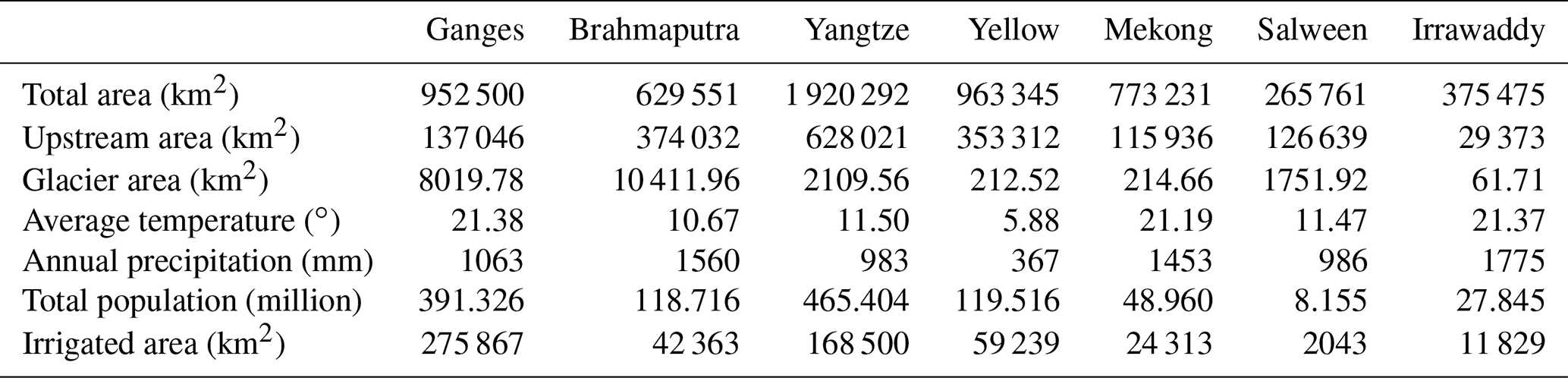
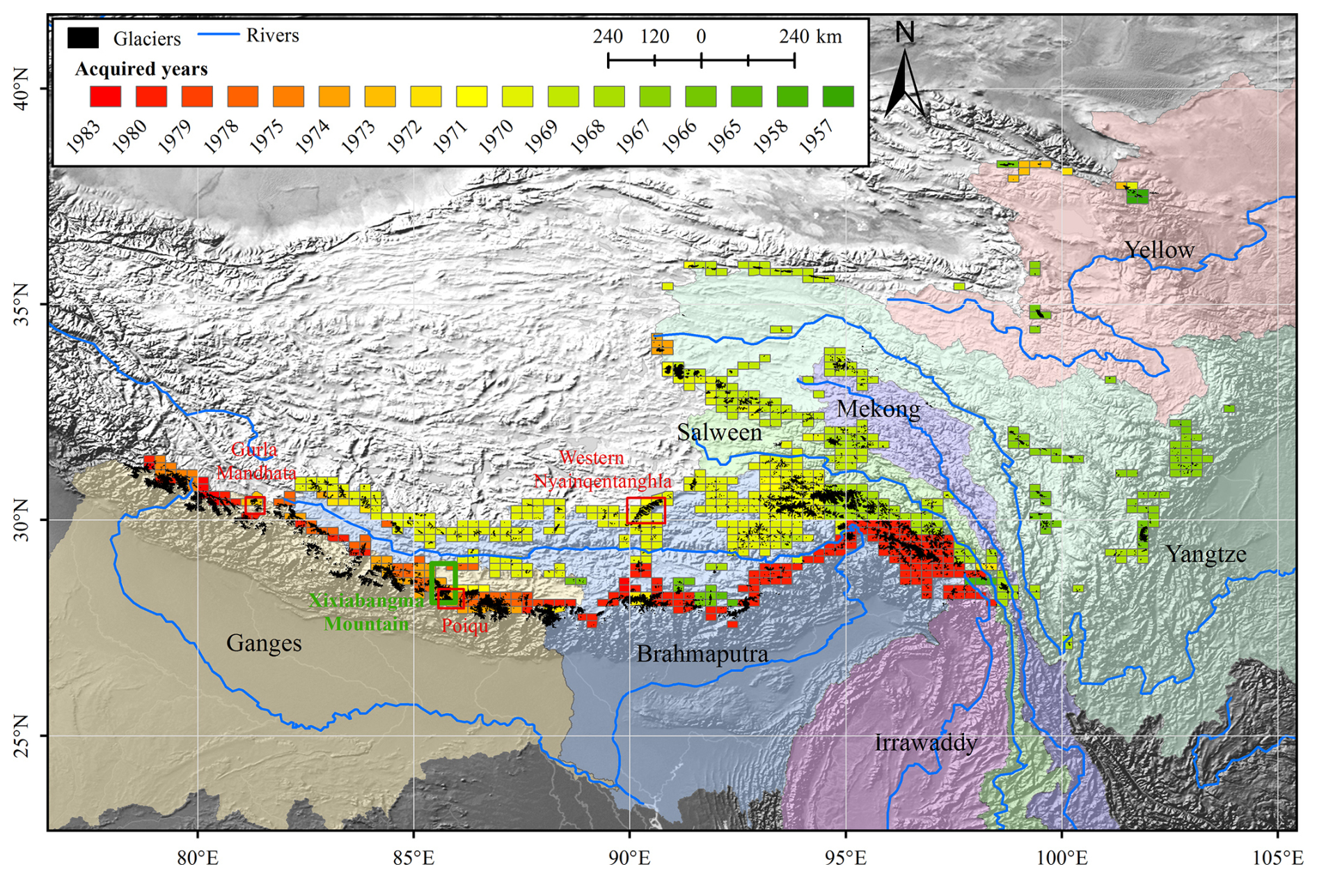
Figure 1 Glaciers in the ETPR and coverage of the topographic maps. The maps were generated from aerial photos acquired from 1957 to 1983. The red- and green-edged rectangles denote specific regions used for product comparison between our dataset and others.

The Yangtze, Yellow, Lancang–Mekong, Salween (Nu Chiang), Irrawaddy, Ganges, and Brahmaputra rivers originate from the eastern and southern Tibetan Plateau and the Himalayas, collectively referred to as the extended eastern Tibetan Plateau region (ETPR) throughout this paper. These rivers make a significant contribution to the water supply of millions of people (Table 1 and Fig. 1) (Immerzeel et al., 2010). Data from the Randolph Glacier Inventory (RGI 6.0) indicate that there are over 23 000 glaciers in the source areas of these rivers, encompassing a total area of 22 782 ± 683 km² (Pfeffer et al., 2014). Meltwater from these glaciers, along with precipitation and snowmelt, sustains river flow. Although glacier runoff is not the primary factor driving water scarcity in most basins of the ETPR, it can partially and temporarily alleviate water resource deficits during drought periods (Gascoin, 2023; Pritchard, 2019). Glaciers in the ETPR exhibit high sensitivity to temperature fluctuations, particularly when ice reaches the pressure melting point, leading to accelerated ablation rates (Shi et al., 1988). Glacier retreat in the region over the past 3 decades is well-documented (e.g., Zhang et al., 2012; Xu et al., 2018; Liu et al., 2019; Wu et al., 2020), with substantial and accelerating reductions in area, length, and thickness. This trend is likely driven by rising temperatures and a complex interplay of factors influencing ablation rates (Table 1). These factors include variations in weather patterns (Table 1), diverse topography (Hewitt, 2011), and the distribution of surface and surrounding features such as debris cover, ponds, crevasses, and proglacial lakes (Scherler et al., 2011; Watson et al., 2018; King et al., 2019). These combined factors pose a significant challenge to accurately evaluating and understanding glacier meltwater dynamics.

Elevation differences derived from the comparison of digital elevation models (DEMs) form an effective approach for assessing glacier mass balance (e.g., Bamber and Rivera, 2007). Recent research based on remote sensing data has enabled substantial advances in quantifying glacier mass changes after 2000. Some studies utilizing the declassified spy satellite data and topographic maps have extended analyses back to the 1970s for specific regions in HMA, providing insights into the glacier mass balance prior to 2000 (Maurer et al., 2019; Ye et al., 2015). However, inconsistencies arising from variations in data sources hinder robust comparisons of glacier mass changes across the region (Shean et al., 2020; Hugonnet et al., 2021; Zhao et al., 2022). Furthermore, the limited availability of pre-2000 data for many glaciers restricts comprehensive assessments of long-term mass changes and their sensitivity to climate change. This scarcity is particularly pronounced for the accumulation zones, where data voids within pre-2000 DEMs (e.g., Keyhole-9 Hexagon, KH-9) introduce uncertainties that compromise the accuracy of glacier contribution estimates of downstream water resources and sea-level rise (Bhattacharya et al., 2021; Zhou et al., 2018). Additionally, there is a scarcity of gridded mass balance products derived from the aggregation of glacier-level mass balance data at specific grid resolutions (e.g., 0.5°) that could serve energy balance and hydrological simulations in a large glacierized basin in the ETPR before 2000. We therefore aim to (1) generate a glacier-level and gridded mass balance dataset from the 1970s to 2000 based on the historical topographic maps (hereafter “Topo” maps) and the Shuttle Radar Topography Mission (SRTM) DEM and (2) provide a comprehensive view of the mass balance across the source area of the ETPR.

2 Data and methods

2.1 Topographic maps

We employed a total of 718 historical topographic maps, including 142 at a scale of 1:50 000 and 576 at a scale of 1:100 000, compiled from aerial photographs taken between 1957 and 1983 by the Chinese Military Geodetic Service (Fig. 1). These maps are referenced to the 1954 Beijing Geodetic Coordinate System, which uses a datum based on the mean sea level of the Yellow Sea as observed at Qingdao Tidal Observatory in 1956. The vertical accuracy of the topographic maps meets the National Photogrammetrical Standard of China (NPSC, GB/T 12343.1-2008). Specifically, the vertical error is less than 5 m on slopes less than 6° and ranges from 5 to 8 m on slopes between 6 and 25°. By using a Helmert transformation (also known as a seven-parameter transformation method), all scanned maps were rectified based on gridded points of the meridians and wefts. Geometric accuracy is controlled by over 600 ground control points measured by the State Bureau of Surveying and Mapping from 1950 to 1990. Subsequently, the contours and other layers were manually digitized on-screen with the 1954 Beijing Geodetic Coordinate System. These digital maps were then transformed into the coordinate system of the SRTM, i.e., the World Geodetic System 1984 (WGS84)/Earth Gravity Model 1996 (EGM96). To generate DEMs, the digital contours were first used to build triangulated irregular networks (TINs), and then the TINs were transformed to gridded elevation products with the natural-neighbor smoothing and interpolation method. The Topo DEMs were finally resampled to 30 m resolution to match the resolution of the SRTM DEM. The uncertainties of Topo DEMs may arise from operator proficiency during map generation, limitations in extracting elevation data from areas with low-contrast features such as snow cover or shadows, and horizontal positioning errors. We will discuss these uncertainties in Sect. 4.2.

Based on the historical topographic maps, the first Glacier Inventory of China (CGI1) was compiled by more than 50 experienced technicians to display the status of glaciers before 2000 (Shi, 2008). Limited by less sophisticated techniques and the scarcity of high-resolution satellite imagery, the first version has a margin of error in glacier area exceeding 10 %. To improve the accuracy of CGI1, the work group of the second Glacier Inventory of China (CGI2) evaluated and refined the CGI1 glacier outlines using the advanced technology employed for CGI2. The revised CGI1 was used for processing the elevation differences in this study.

2.2 SRTM

The SRTM provides C- and X-band topographic data in February 2000 with 1 and 3 arcsec special resolutions (Farr et al., 2007). Previous studies have pointed out that the accuracy of the SRTM (C-band) DEM presented a high level (−5.61 ± 15.68 m) for high relief (Carabajal and Harding, 2006). In glacierized regions, the elevation bias can be up to 10 m at high altitudes (Berthier et al., 2006). In this study, we use the SRTM DEM (no-void filled version) with a resolution of 1 arcsec (∼ 30 m), referring to the glacier surface in the year of 1999 suggested by previous studies (e.g., Gardelle et al., 2013; Mcnabb et al., 2019). In addition, the limited X-band DEM data (Hoffmann and Walter, 2006) have been employed to quantify the underestimation of elevations in C-based DEMs caused by penetration of microwaves. All of the datasets are downloaded from http://earthexplorer.usgs.gov/ (last access: 2 January 2025).

2.3 KH-9 data

The KH-9 images, declassified in 2002, were acquired by Cold War spy satellites with a flight height of approximately 170 km from 1971 to 1986. In this study, we acquired KH-9 images covering Xixiabangma. To generate a DEM, reseau grids overlaid on the KH-9 images were initially used to reconstruct the original geometry (Pieczonka et al., 2013). Subsequently, surrounding pixels were utilized to fill the grid areas, followed by image enhancement techniques, including histogram equalization and Wallis filtering. Manual identification of GCPs is a conventional method for estimating unknown camera positions and orientations, typically for a few selected image pairs (Pieczonka et al., 2013). In this study, 26 evenly distributed GCPs were selected from reference images (Landsat ETM+ images for horizontal orientation and the SRTM for vertical orientation) to correct the external orientation of the KH-9 images. Several tie points in glacier regions were added manually to improve the matching accuracy. By considering the focal length (∼0.3 m for 1973–1980), flight height, and film size ($\sim \mathrm{0.23}\times \mathrm{0.46}$ m), the DEMs were finally generated. In some cases (e.g., Bhattacharya et al., 2021), a physical model was used to compensate for the unclassified (or unknown) imaging parameters (e.g., lens distortion). In addition, we obtained elevation difference products from KH-9 and the SRTM published by Bhattacharya et al. (2021). These datasets were used to evaluate the performance of elevation differences derived from the Topo DEMs.

2.4 Ice, Cloud, and land Elevation Satellite-2 (ICESat-2) data

ICESat-2, launched in 2018, is the second spaceborne laser altimetry mission which aims to estimate ice sheet mass changes, lake volume, and global vegetation heights (Markus et al., 2017). Similar to ICESat-1, ICESat-2 acquires the distance between the sensor and Earth's surface by recording the travel time of laser pulses, which are sent out by the Advanced Topographic Laser Altimetry System (ATLAS) – a photon-counting 532 nm (green-light) lidar operating at 10 kHz. The system splits the laser pulse into six beams forming three pairs (a weak beam and a strong beam separated by 90 m, included in one pair) to make an accurate measurement of surface height. It takes 91 d to complete a full orbital cycle (1387 unique reference ground tracks) (Smith et al., 2019). ICESat-2 boasts denser ground footprints compared to ICESat-1 due to its smaller footprint diameter (∼ 17 m) and reduced along-track offset (∼ 0.7 m) for each laser beam. The photon geolocation information is aggregated at 40 m along-track length scales.

2.5 Coregistration and potential systematic error correction for derived elevation differences

2.5.1 Coregistration between DEMs

There are both horizontal and vertical offsets in the two coregistered DEMs due to dataset sources and the method used in the production of DEMs (Paul, 2008). These shifts can be corrected by using an iterative coregistration method implemented by Nuth and Kääb (2011). In this method, the elevation differences in a static off-glacier surface between two DEMs (defined as dh) were correlated with the slope and aspect of the surface (Nuth and Kääb, 2011; Berthier et al., 2007). The relationship can be quantified by Eq. (1):

$$\begin{array}{}\text{(1)}& \text{dh}=a\times \cos (b-\mathit{\phi })\times \tan \left(\mathit{\alpha }\right)+\stackrel{\mathrm{‾}}{\text{dh}},\end{array}$$

where φ is the aspect, α is the slope, $\stackrel{\mathrm{‾}}{\text{dh}}$ is the vertical offset of the registered DEM, and a and b represent the horizontal offset and direction, respectively.

DEMs generated from aerial or satellite imagery are susceptible to rotational errors due to limitations in absolute accuracy. The coregistration method of Nuth and Kääb (2011) does not account for such errors. Consequently, a complementary correction, such as deramping or iterative closest-point (ICP) registration (Besl and Mckay, 1992), is required. In the current study, we defined the SRTM DEM as the reference DEM. The off-glacier region was identified as a static surface which was assumed to be stable during the study period (1970s–2000). It should be noted that the processes for registration and correction of the Topo DEM were applied at a group scale rather than a map scale. Every group including at least one Topo DEM should cover all glaciers in an independent mountain range. This group-scale processing strategy for generating elevation differences minimizes errors caused by glacier extents exceeding individual map sheet boundaries. There is a total of 261 groups in the ETPR. By conducting the coregistration, the resulting horizontal translation was applied to the Topo DEMs of each group, and the median vertical bias was removed. Subsequently, we performed a second-order deramping for correction of possible rotations. The deramping method works by estimating and correcting for an N-degree polynomial over all the differences between a reference DEM and the DEM to be aligned. Biases caused by different spatial resolutions between the DEMs could be adjusted by the relationship between elevation differences and maximum curvatures (Gardelle et al., 2012). The application of all corrections improved the accuracy of derived elevation differences in off-glacier regions, as evidenced by both the histogram statistics (Fig. S2) and the reduction in the median and normalized median absolute deviation (NMAD) shown in Table S1 in the Supplement compared to the values observed before applying corrections.

The corrected elevation differences with values exceeding ± 150 m were assumed to be obvious outliers and were removed (Bhattacharya et al., 2021; Pieczonka and Bolch, 2015). There were still some unrealistic phenomena, such as large surface thinning in accumulation zones, which are typical of Hexagon KH-9 elevation changes (Zhou et al., 2018). These outliers were attributed to inaccurate matching of DEMs and can be removed by using an elevation-dependent sigmoid function (Eq. 2) (Zhou et al., 2018; Pieczonka and Bolch, 2015):

$$\begin{array}{}\text{(2)}& \mathrm{\Delta }{\text{dh}}_{max}={\left({\displaystyle \frac{h_{max}-h_{\text{gla}}}{h_{max}-h_{min}}}\right)}^{\mathrm{2}}\times A,\end{array}$$

where Δdh_max represents the maximum elevation change; h_max, h_min, and h_gla are the maximum, minimum, and pixel-level elevations, respectively; and A is the maximum elevation change occurring within 150 m of each glacier terminus. Following outlier removal, normalized regional hypsometric interpolation was employed to fill the remaining data gaps. Notably, the original, non-interpolated elevation difference data were retained in the final product to ensure data integrity. For glacier-scale product generation, the inclusion of a glacier in the mass balance calculation was determined using the non-interpolated elevation difference data.

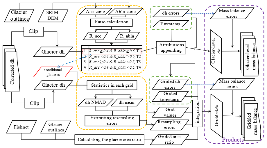
Figure 2 Workflow diagram for glacier-level and gridded product generation. The yellow dashed boxes represent the key steps involved in producing data products. The two green dashed boxes are connected to indicate that gridded attributes are derived from glacier-level attributes. The purple dashed box represents the product integration stage, while the red dashed box highlights the conditions used to select valid glaciers.

2.5.2 Penetration depth estimation and correction of the SRTM DEM

DEMs derived from the SRTM C-band contain biases due to the penetration of microwaves into dry snow, firn, and ice (Rignot et al., 2001). Because of the narrow swath widths and limited available data (see Fig. S3), it is hardly possible to use the X-band DEM (e.g., Hoffmann and Walter, 2006; Dehecq et al., 2016) to calculate the elevation difference. We therefore used the X-band DEM to evaluate the penetration depth of the C-band DEM (C_penetration). The penetration depth was estimated in the glacierized areas by comparing the SRTM C-band and X-band DEM data. To extend our results to the entire study area despite incomplete data coverage, we employed a limited-data fitting approach to establish a relationship between penetration depth and altitude. This relationship was then applied to all of the data. The results revealed an average penetration depth ranging from 3.8 to 6.2 m across the elevation range (Fig. 2 and S4). While penetration depth increases with a longer radar wavelength (Curlander and Mcdonough, 1991), this does not imply that the X-band DEM presents no penetration effects. While some studies suggest that this penetration depth is often negligible for estimating elevation changes over a decade, in the Qinghai–Tibet Plateau, it can exceed 2 m (Li et al., 2021), potentially influencing elevation differences.

The calculated penetration depth above represents the difference between C-band and X-band radar. To account for X-band penetration, the study employed results from Zhou et al. (2022), who calculated X-band penetration in the subregion of the ETPR using the TerraSAR-X add-on for Digital Elevation Measurement (TanDEM-X) and Pléiades DEMs with an acquisition time difference of only 4 d. Their results were used to fit a relationship between penetration depth (X_penetration) and altitude (ele), as shown in the following equation:

$$\begin{array}{}\text{(3)}& X_{\text{penetration}}=\text{ele}\times \mathrm{0.0068}-\mathrm{34.3368}.\end{array}$$

This relationship was applied for X-band penetration correction. Ultimately, the C-band DEM-based penetration depth used in the study is the sum of the calculated C-band–X-band difference (CX_diff) and the X-band penetration.

2.6 Uncertainty estimation

2.6.1 Uncertainties in elevation difference estimation

DEMs are inherently susceptible to large-scale instrument noise and variable vertical precision, resulting in complex error patterns. Accuracy and precision have been used to describe these errors. Precision pertains to random errors, whereas accuracy addresses systematic errors and, in some instances, both systematic and random errors (Hugonnet et al., 2022). In many cases of studies on glacier elevation changes, the stable terrain was used to evaluate uncertainties in DEMs (Shean et al., 2020; Zhou and Duan, 2024). However, most of the previous studies largely underestimated uncertainties in DEMs due to insufficient consideration of spatial correlation errors, particularly long-range spatial correlations. In this study, we leverage the comprehensive uncertainty assessment framework proposed by Hugonnet et al. (2022) to estimate uncertainties in our Topo DEMs.

Systematic biases in the differences of DEMs were addressed through coregistration and penetration correction using SRTM C-band data. Outlier removal further eliminated any remaining biases in glacierized areas. Uncertainties in the corrected elevation differences stem primarily from two aspects, i.e., heteroscedasticity of elevation measurements and spatial correlation of errors (Hugonnet et al., 2022). Throughout the assessment, the median was employed as a robust estimator of the central tendency, while the NMAD served as a measure of statistical dispersion.

$$\begin{array}{}\text{(4)}& \text{NMAD}=\mathrm{1.4826}\cdot \text{median}(\mathrm{|}{\text{dh}}_i-\text{median}(\text{dh}\left)\mathrm{|}\right)\end{array}$$

dh denotes the full sample of per-pixel difference values between the Topo and SRTM DEM surfaces after coregistration.

Elevation heteroscedasticity was estimated by sampling the empirical dispersion of elevation differences. The NMAD was employed to quantify dispersion within binned categories defined by terrain slope and maximum absolute curvature. Based on this analysis, a functional relationship between the variance of elevation differences (σ_dh), terrain slope (α), and maximum absolute curvature (c) was established as f=σ_dh(αc). The error for each pixel was estimated by using this function.

To mitigate the influence of heteroscedasticity on spatial autocorrelation analysis of residual errors in the Topo DEM products, we standardized the elevation differences using the error map. This procedure aligns with Eq. (12) in Hugonnet et al. (2022) and enhances the robustness of error estimation by removing variability in variance caused by heteroscedasticity. Subsequently, we sampled empirical variograms (Eq. 5) for standard elevation difference maps between the Topo and reference DEMs over stable surfaces using Dowd's estimator (Dowd, 1984):

$$\begin{array}{}\text{(5)}& \mathrm{2}{\mathit{\gamma }}_{\text{dh}}\left(d\right)=\mathrm{2.198}\cdot \text{median}{\left(z_{\text{dh}}(x,y)-z_{\text{dh}}(x^{\prime },y^{\prime })\right)}^{\mathrm{2}},\end{array}$$

where d is the spatial lag between locations (x,y) and $(x^{\prime },y^{\prime })$ and z_dh is the standard elevation difference, which can be calculated by $\text{dh}/{\mathit{\sigma }}_{\text{dh}}\left(\mathit{\alpha }c\right)$.

For each difference map group, we employed a variogram analysis to characterize the spatial autocorrelation of residuals. This involved sampling and averaging 10 unique variograms, each with a sample size of 5000 pixels. We fit two nested variogram models to the empirical variograms using weighted least squares: a Gaussian model at short ranges and a spherical model at long ranges. This combination yielded the smallest least-square residuals for most map groups. In some cases, a double-range nested spherical variogram model provided a better fit. Finally, the spatially integrated uncertainties (${\mathit{\sigma }}_{\stackrel{\mathrm{‾}}{\text{dh}}}$) for elevation differences within a specific area, such as a glacier, can be calculated using the following equation:

$$\begin{array}{}\text{(6)}& {\mathit{\sigma }}_{\stackrel{\mathrm{‾}}{\text{dh}}}={\displaystyle \frac{{\mathit{\sigma }}_{\text{dh}}}{\sqrt{N}}},\end{array}$$

where σ_dh is the vertical precision of the samples in the specific area, and N is the number of independent pixels in the specific area based on the spatial correlations modeled by γ_dh. The solution for N can be found by referring to the Methods section in the Supplement of Hugonnet et al. (2022).

2.6.2 Uncertainties in mass balance estimation

The annual surface elevation changes ($\frac{\partial \text{dh}}{\partial t}$) were converted to mass balance (mb) using Eq. (7). A standard bulk ice density of ρ = 850 kg m⁻³ (Huss, 2013) was applied to assess the water equivalent.

$$\begin{array}{}\text{(7)}& \text{mb}={\displaystyle \frac{\partial \text{dh}}{\partial t}}\times \mathit{\rho }\end{array}$$

The uncertainties included in the glacier area and glacier density should be taken into account in the estimation of the mass balance uncertainty. The uncertainty in the glacier area is reported as approximately 8 % for South Asia (Pfeffer et al., 2014), accounting for the temporal evolution of glacier extent and glacier boundary mapping. Referring to the study of Huss (2013), the density uncertainty can be assumed to be Δρ = 60 kg m⁻³. Considering all uncertainties to be uncorrelated, we can estimate the total uncertainty in mass balance using Eq. (8).

$$\begin{array}{}\text{(8)}& \mathit{\sigma }M=\sqrt{{\left({\displaystyle \frac{\text{dh}}{t}}\times {\displaystyle \frac{\mathrm{\Delta }\mathit{\rho }}{{\mathit{\rho }}_{\mathrm{w}}}}\right)}^{\mathrm{2}}+{\left({\displaystyle \frac{\sqrt{{\mathit{\sigma }}_{\stackrel{\mathrm{‾}}{\text{dh}}}^{\mathrm{2}}+{\left(\frac{\mathit{\sigma }A}{A}\right)}^{\mathrm{2}}}}{t}}\times {\displaystyle \frac{\mathit{\rho }}{{\mathit{\rho }}_{\mathrm{w}}}}\right)}^{\mathrm{2}}}\end{array}$$

dh is the glacier thickness change, t denotes the observation period, ρ_w is the density of water (999.972 kg m⁻³), and σA and σρ are the glacier area uncertainty and density uncertainty, respectively.

In the evaluation of total regional mass loss, this is critical for incorporating additional error propagation steps transitioning from the glacier scale to the regional scale. This is necessitated by the fact that, once uncertainties are aggregated from a smaller spatial support (e.g., individual pixels) to a larger spatially contiguous ensemble, they can subsequently be propagated to an even broader ensemble (e.g., all glaciers within a region), in accordance with Krige's transitivity relation (Webster and Oliver, 2007; Hugonnet et al., 2022). In this study, the evaluation was conducted using Eq. (20) of Hugonnet et al. (2022). The errors associated with elevation differences at the regional, basin, and gridded scales were assessed using xDEM (Hugonnet et al., 2024). For errors related to density or area, a 100 % correlation at the regional scale was generally assumed, and the mean errors in density or area were applied. Finally, Eq. (8) was recalculated to determine the mass balance error at the regional scale. Throughout the paper, uncertainties in elevation difference and mass balance are presented at the 95 % confidence level (2σ).

2.7 Development of the glacier-level and gridded mass change datasets

Utilizing the final elevation difference data, we extracted the elevation change results for each glacier by clipping to the CGI1 glacier boundary. Subsequently, we filtered the glaciers to eliminate erroneous estimates of glacier elevation change due to incomplete topographic map coverage. To achieve this, we defined coverage ratios (R_acc and R_abla) for the accumulation and ablation zones, respectively. These ratios represent the proportion of the coverage area of the elevation difference compared to the total area of the accumulation or ablation zones of a glacier. The accumulation and ablation zones for a specific glacier are identified by equilibrium line altitude (ELA), which was defined as the median surface elevation of a glacier referring to Sakai et al. (2015). Glaciers with coverage ratios of R_acc ≥ 0.4 (accumulation zone) and R_abla ≥ 0.5 (ablation zone) were classified as “effective glaciers” and included in the final glacier-level product and subsequent analyses. These thresholds were established to ensure sufficient data coverage within each zone for reliable estimates of glacier mass balance. In total, 13 117 out of 24 869 (∼ 52 %) glaciers met this criterion (∼ 27 % of glaciers lack any topographic map coverage). Notably, even though the number of effective glaciers represents a small percentage, their total area coverage accounts for ∼ 72 %. With the selection of effective glaciers, we proceeded to generate the initial glacier-level product. To facilitate the calculation of the glacier mass balance, we created a time layer based on the acquisition date of each topographic map. This time layer accounts for potential differences between pixels within a glacier since a glacier may be divided into several parts by Topo maps, although this is rare. In our products, the time layer distinguishes between these differences. Additionally, within the attributes of each glacier elevation product, we provided the average elevation change for the glacier, the number of effective pixels (N) characterizing spatial autocorrelation, and the final elevation change error ${\mathit{\sigma }}_{\stackrel{\mathrm{‾}}{\text{dh}}}$ (computed based on Sect. 2.6).

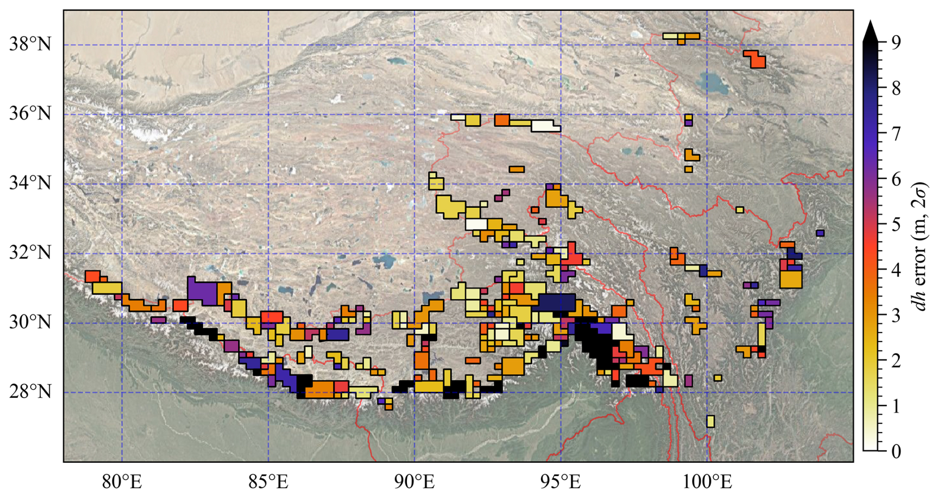
Figure 3 Spatial distribution of the glacier surface elevation change error (2σ) from the 1970s to 2000. The polygons represent groups. The base map depicted in the image utilizes Google Terrain Map (©Google Maps 2024), accessed through Python for visualization.

Table 2 Statistics of vertical errors in each basin.

Compared with the glacier-level products, the primary challenge for gridded datasets lies in ensuring the representativeness of the elevation difference within each grid rather than relying solely on coverage ratios. This means that a large number of samples are required for a specific grid, especially for grids with large sizes (e.g., 0.5°). However, most of the studies fall short of this requirement due to sparse image coverage across large regions. These studies often estimate the glacier mass balance for a large-scale region using data from one or several small glacierized areas located within the broader region (e.g., Pieczonka and Bolch, 2015; Bhattacharya et al., 2021). Fortunately, the comprehensive topographic map coverage employed in this study ensures a sufficient number of samples for producing the gridded product. To achieve gridded product generation, we follow the following steps: (1) we begin by spatially merging the elevation difference, elevation difference error, and time stamps for all effective glaciers. (2) For each grid cell, we calculate the average of the glacier elevation difference, elevation difference error, and time stamps within that grid cell. These averaged values are assigned as the grid cell values. (3) For each grid cell, we compute the NMAD of the elevation difference and the number of pixels. Using Eq. (6), we calculate the grid-scale resampling error. (4) Combining the grid-scale elevation difference and time stamps, we apply Eq. (7) to calculate the grid-scale mass balance. (5) Combining the grid-scale elevation change error and time stamps, we apply Eq. (8) to calculate the initial grid-scale mass balance error. Finally, we incorporate the resampling error to obtain the final mass balance error.

The processing flowchart for the glacier-level and gridded datasets can be found in Fig. 2.

3 Results

3.1 Uncertainties

The spatial average error in the glacier elevation difference is 4.28 m (2σ). Considering the time difference between the acquisition dates of the topographic maps, the average annual error in glacier elevation change for the entire study area is 0.15 m. Considering the uncertainty in glacier area and density, an average uncertainty of 0.13 m (2σ) for the mass balance in the study area can be calculated using Eq. (8). The average error in the elevation difference for the 0.5° product is 3.36 m (2σ). This translates into an error of 0.11 m in the glacier mass balance. While there is a slight difference in the error between the two products, the overall results are relatively close. This difference may be attributed to errors arising from resampling.

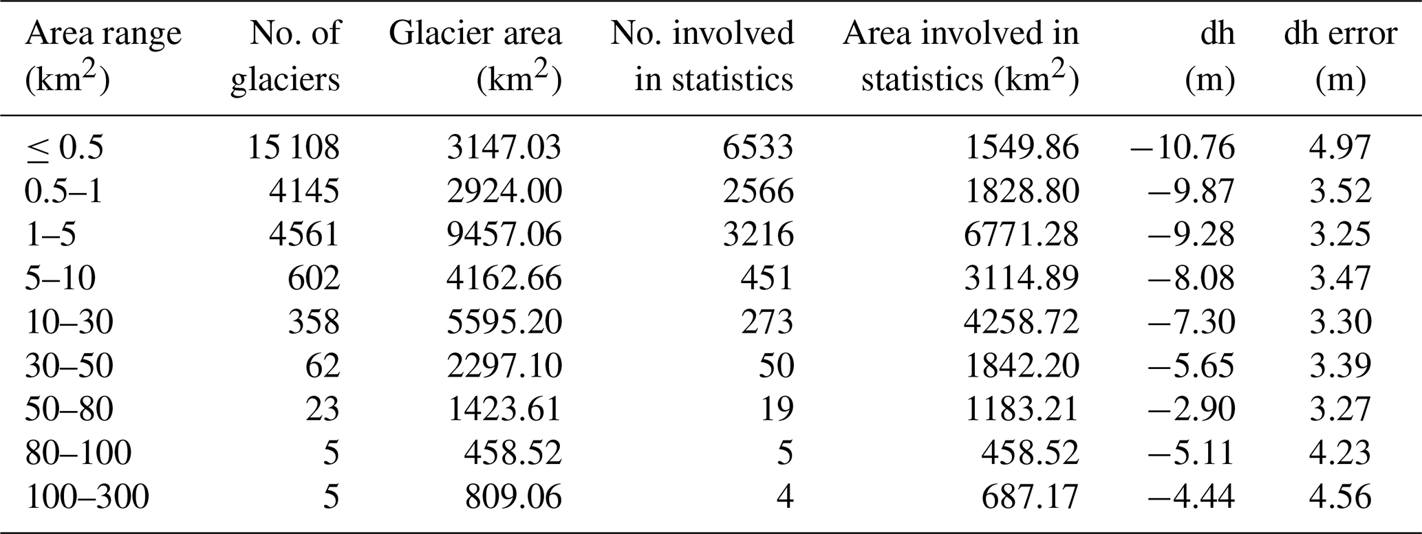
Table 3 The statistics of elevation difference (dh) for different glacial scale. The standard scale range for glaciers refers to Shi et al. (1988).

Figure 4 Elevation difference of large glaciers (> 10 km²) by aspect and slope.

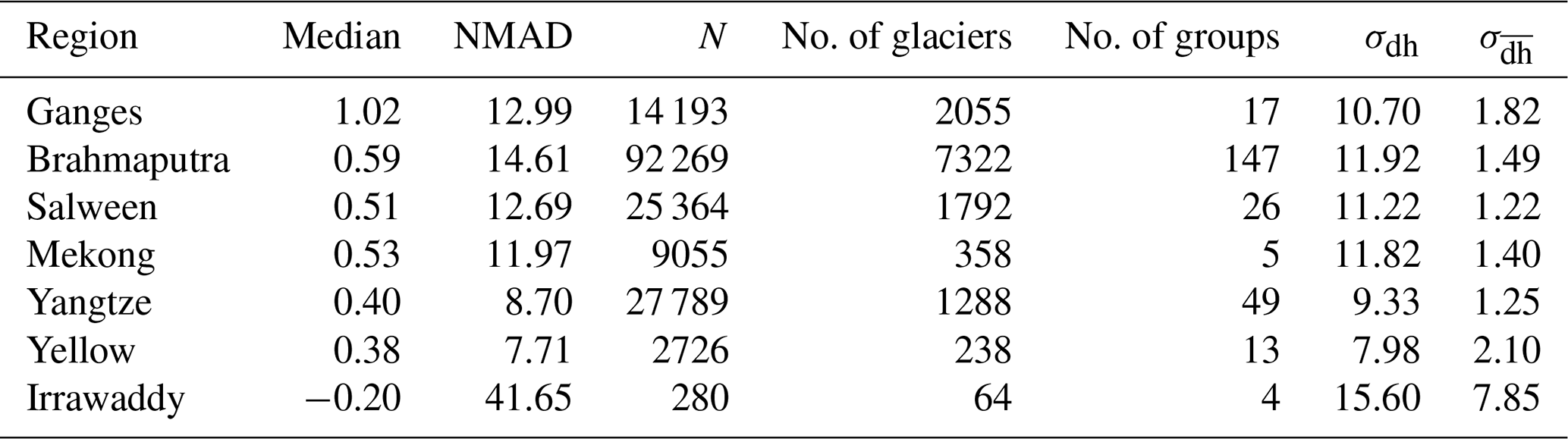
Uncertainties exhibit significant spatial heterogeneity. The Ganges basin and the junction of the Brahmaputra and Salween basins show larger uncertainties, as shown in Fig. 3. This spatial variation is further supported by basin-level analysis of elevation difference uncertainty data (Table 2). The Irrawaddy basin exhibits the largest error, followed by the Ganges. These spatial differences can be partially explained by analyzing the elevation difference for off-glacier areas. As illustrated in Fig. S5, the median and NMAD of the elevation change reveal these variations. However, the primary contributor to this spatial heterogeneity is likely spatial autocorrelation in elevation change, particularly long-range correlations (Fig. S6).

Despite implementing the processing at the group level, glaciers within the same group exhibit varying errors. This variation arises from two key factors: inherent pixel-level errors associated with the elevation heteroscedasticity for each glacier and the number of effective pixels calculated by spatial distances of long-range and short-range correlations used to represent each glacier (see the dataset attributes).

3.2 Glacier-level mass change

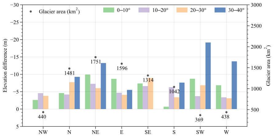
The area involved in statistics accounts for 72 % of the total glacierized area. The average elevation difference for the period from the 1970s to 2000 was −9.52 ± 4.28 m, corresponding to a mass balance of −0.30 ± 0.13 $\mathrm{m}\mathrm{w}.\mathrm{e}.{\mathrm{yr}}^{-\mathrm{1}}$. Small glaciers showed more negative mass change than large glaciers. As glacier size increases, the rate of surface thinning diminishes. However, the thinning of larger glaciers is subject to greater uncertainty (Table 3). Uncertainties in surface thickness change range from 0.35 to 31.98 m for the study period. Detailed information on these uncertainties can be found in the glacier-level dataset. Large glaciers are becoming increasingly crucial as they are expected to persist for a longer duration compared to smaller glaciers, which are continuously disappearing due to the relentless effects of climate change. To gain a deeper understanding of elevation changes in large glaciers, we conducted statistical analyses on glaciers with an area exceeding 10 km² (Fig. 4). The results revealed that the largest thickness reduction (∼ −13.4 m) occurred in the northeastward glaciers, which also hold the largest area proportion. Overall, a correlation was observed between the average slope of the glaciers and the magnitude of surface thinning. However, glaciers facing east and southeast exhibited a somewhat different pattern.

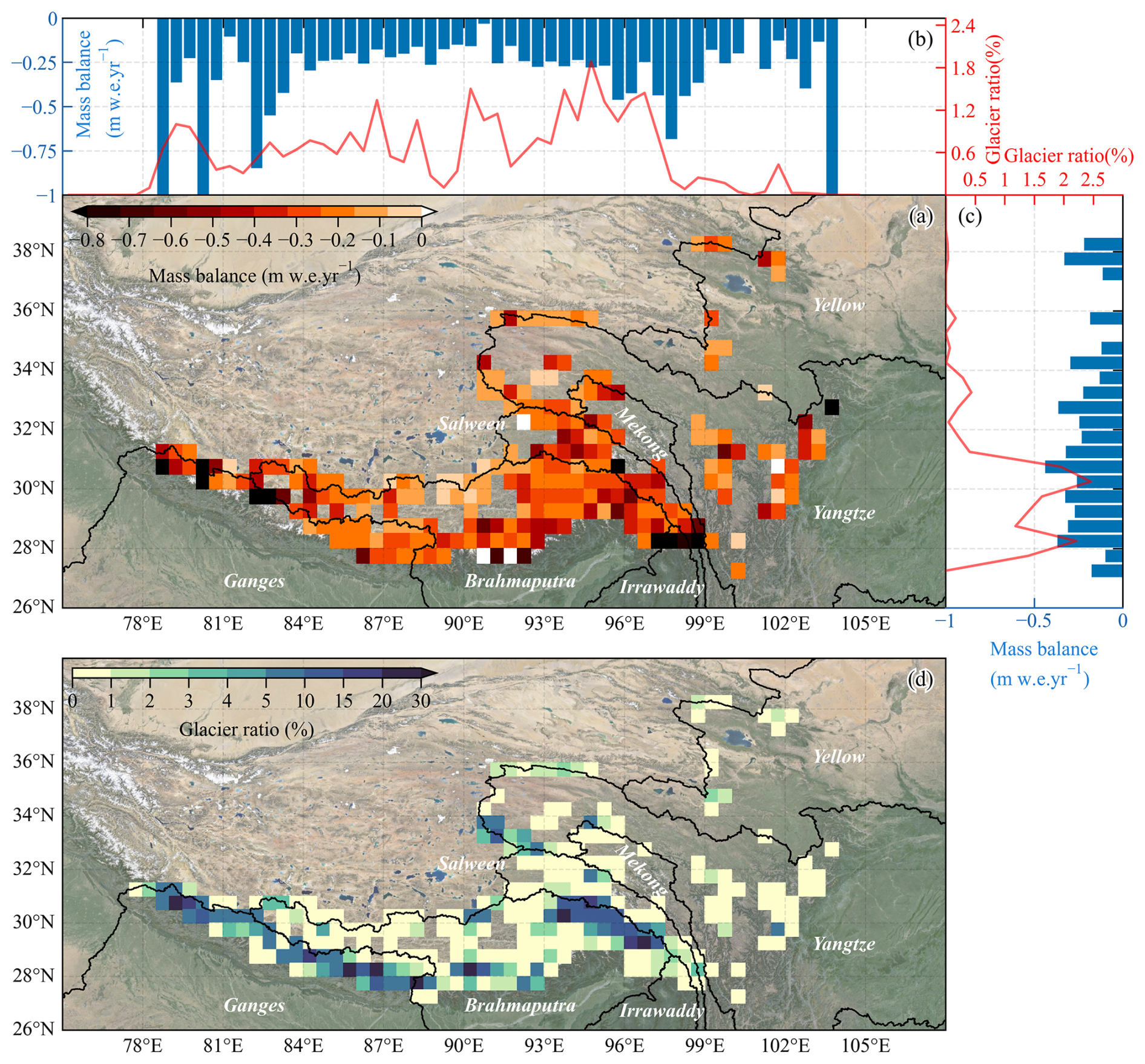
Figure 5 The 0.5° gridded product over the ETPR. (a) Characteristics of glacier mass balance. (d) Glacier ratio. Statistics of the mass balance along longitude and latitude are presented in panels (b) and (c), respectively. The glacier ratio accounts for the glacier area divided by the grid area. The base map depicted in the image utilizes Google Terrain Map (©Google Maps 2024), accessed through Python for visualization.

The Irrawaddy basin exhibited the largest mass loss, with values of about −0.68 $\mathrm{m}\mathrm{w}.\mathrm{e}.{\mathrm{yr}}^{-\mathrm{1}}$. However, this estimate also carries a large uncertainty (Table S4). The Ganges (−0.38 ± 0.19 $\mathrm{m}\mathrm{w}.\mathrm{e}.{\mathrm{yr}}^{-\mathrm{1}}$) and Brahmaputra (−0.30 ± 0.14 $\mathrm{m}\mathrm{w}.\mathrm{e}.{\mathrm{yr}}^{-\mathrm{1}}$) basins, which collectively account for over 80 % of the glacier coverage in the ETPR, exhibit mass balance trends that closely reflect the pattern for the entire study area. The Yangtze River basin, on the other hand, displayed the smallest relative error in its mass balance estimate (−0.22 ± 07 $\mathrm{m}\mathrm{w}.\mathrm{e}.{\mathrm{yr}}^{-\mathrm{1}}$), suggesting higher-quality terrain data coverage in this region.

3.3 Gridded glacier mass balance

This study presents a high-resolution (0.5°) gridded product of glacier elevation change for the ETPR. The developed gridded product offers significant advantages for analyzing spatial patterns of glacier mass balance. The gridded format allows for efficient identification and analysis of “hotspot” regions experiencing significant glacier elevation changes. Moreover, they serve as a critical foundation for characterizing glacier runoff in glacierized basins and calibrating parameters in hydrological models that simulate the meltwater contribution to the total runoff. Glaciers in the ETPR exhibited a mass balance of −0.29 $\mathrm{m}\mathrm{w}.\mathrm{e}.{\mathrm{yr}}^{-\mathrm{1}}$ (corresponding to −9.23 m surface thinning during the study period) at a 0.5° grid scale for the investigated period (Fig. 5). Our analysis reveals minimal and statistically insignificant differences in mass balance estimates due to grid size variations. For example, the 30 m resolution product yielded a surface thinning value of −9.52 m. These negligible discrepancies are likely attributable to the resampling process used to generate the gridded data. Details on resampling procedures are provided with each product for further reference. Our analysis reveals an apparent discrepancy in the glacier mass balance through the meridional and zonal distribution. Specifically, there is a decrease in the mass balance with increasing latitude, and two hotspot regions (the source area of the Brahmaputra and the upper reaches of the Mekong, Salween, and Irrawaddy) exhibit the largest negative mass balance along the meridional direction.

4 Discussions

4.1 Evaluation of the Topo DEM elevation difference

Given the confidentiality and unavailability of topographic maps, directly quantifying the systematic and random errors introduced during map scanning, distortion correction, and DEM generation processes proves exceptionally challenging. Consequently, utilizing stable terrain as a proxy for evaluating the reliability of the Topo DEM has emerged as an alternative approach. This approach involves a comparative evaluation with a DEM generated from KH-9 data acquired around the same temporal window. The well-established credibility of KH-9 data, coupled with their documented application in various studies in HMA (e.g., Zhou et al., 2018; King et al., 2019), strengthens the validity of this comparative strategy.

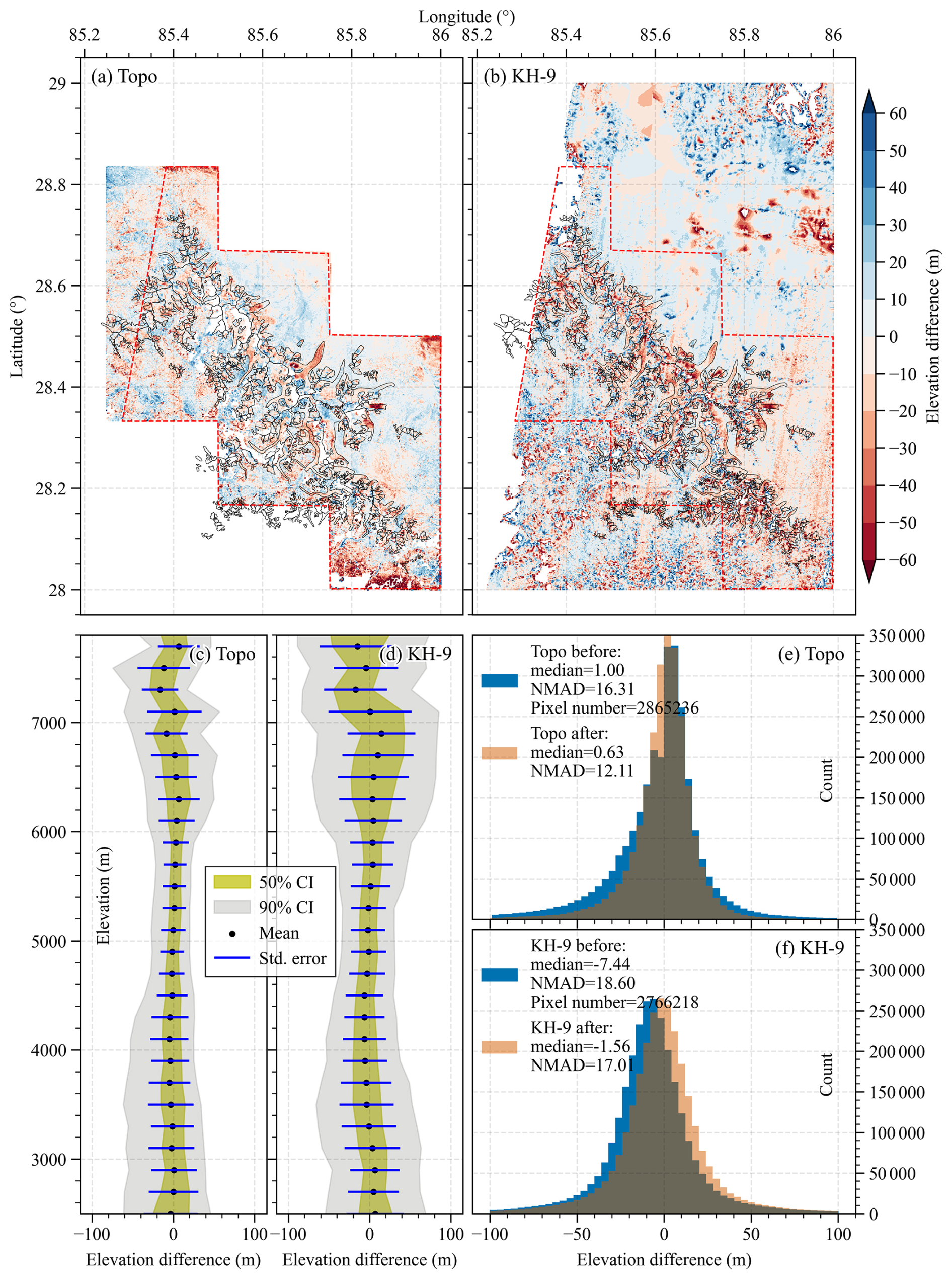
Figure 6 Comparison of (a) Topo-based and (b) KH-9-based elevation differences after coregistration. The statistics on elevation difference along elevation for Topo and KH-9 results are displayed in panels (c) and (d). The frequency distribution of elevation differences for the Topo DEM and the KH-9 DEM is presented in panels (e) and (f), respectively. The CI denotes the confidence interval.

The Xixiabangma mountain range was chosen as the test site due to its near-contemporaneous acquisition times (November 1974) for both datasets and its complex topography representative of the wider ETPR. To minimize the influence of errors introduced during elevation difference extraction, identical processing workflows were applied to both DEMs (details provided in Sect. 2.5), except for the DEM generation method itself. Statistical analyses were performed on approximately 2.8 million off-glacier pixels (Fig. 6). The analysis revealed a broadly similar pattern in elevation differences below 6000 $\mathrm{m}\mathrm{a}.\mathrm{s}.\mathrm{l}.$ for both DEMs. However, discrepancies emerged at higher elevations (above 6000 $\mathrm{m}\mathrm{a}.\mathrm{s}.\mathrm{l}.$). In the 6000–7000 $\mathrm{m}\mathrm{a}.\mathrm{s}.\mathrm{l}.$ range, the Topo DEM exhibited elevation differences close to 0 m, while the KH-9 DEM showed a positive difference. Notably, the large standard deviation (> 40 m) in both cases indicated a low degree of reliability for elevation differences at high altitudes. To quantitatively assess the similarity, we employed histogram statistics. The median and NMAD of the off-glacier elevation differences were calculated before and after the coregistration. The results (Fig. 6e and f) demonstrate a more concentrated distribution centered around zero and a smaller NMAD for the Topo-based elevation difference compared to the KH-9-based elevation difference in stable areas. This suggests that the Topo DEM indicates a higher level of product quality compared to the KH-9 DEM in this region, but this warrants further validation through additional comparative studies and a more comprehensive error characterization of both DEMs.

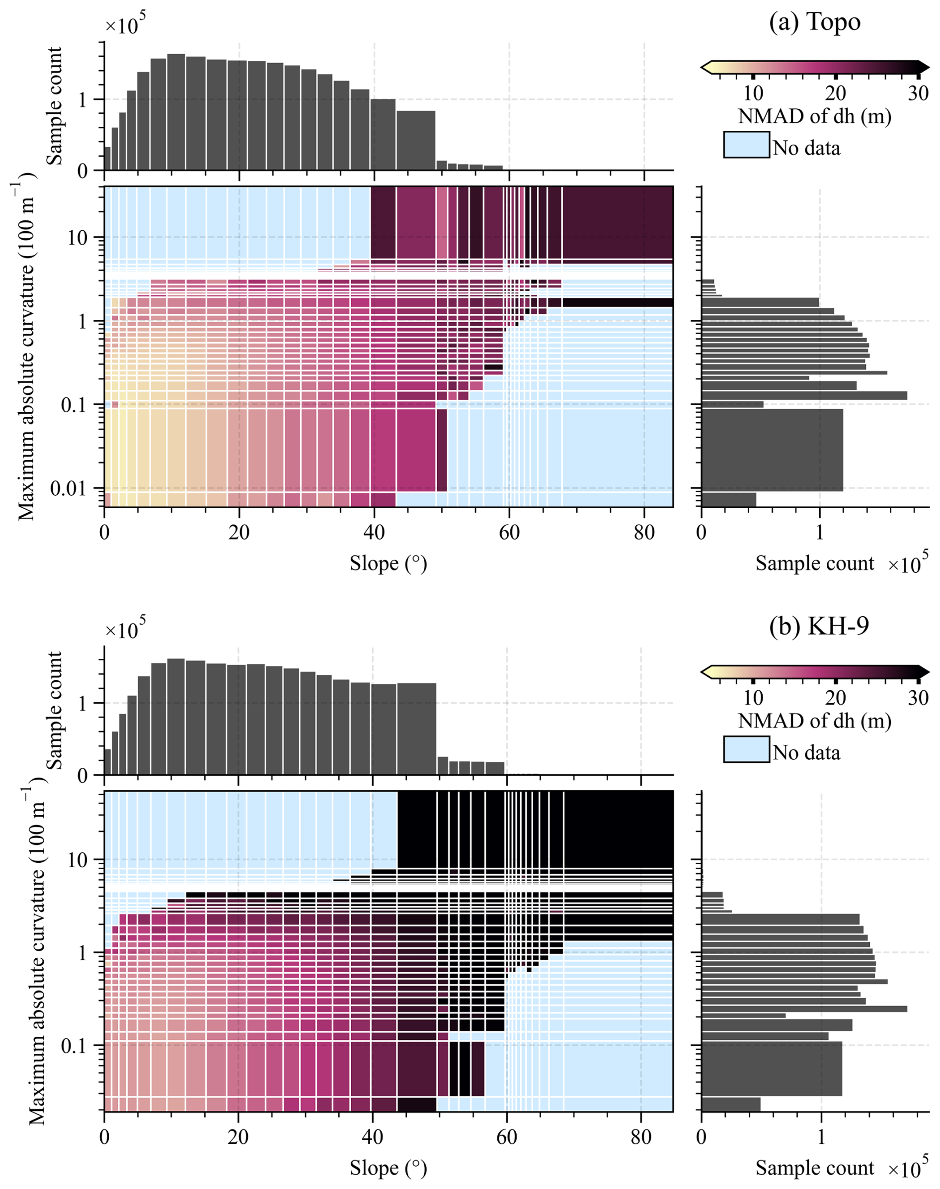
Figure 7 Statistical analysis of off-glacier elevation differences in the Topo DEM (a) and the KH-9 DEM (b) as a function of maximum absolute curvature and slope.

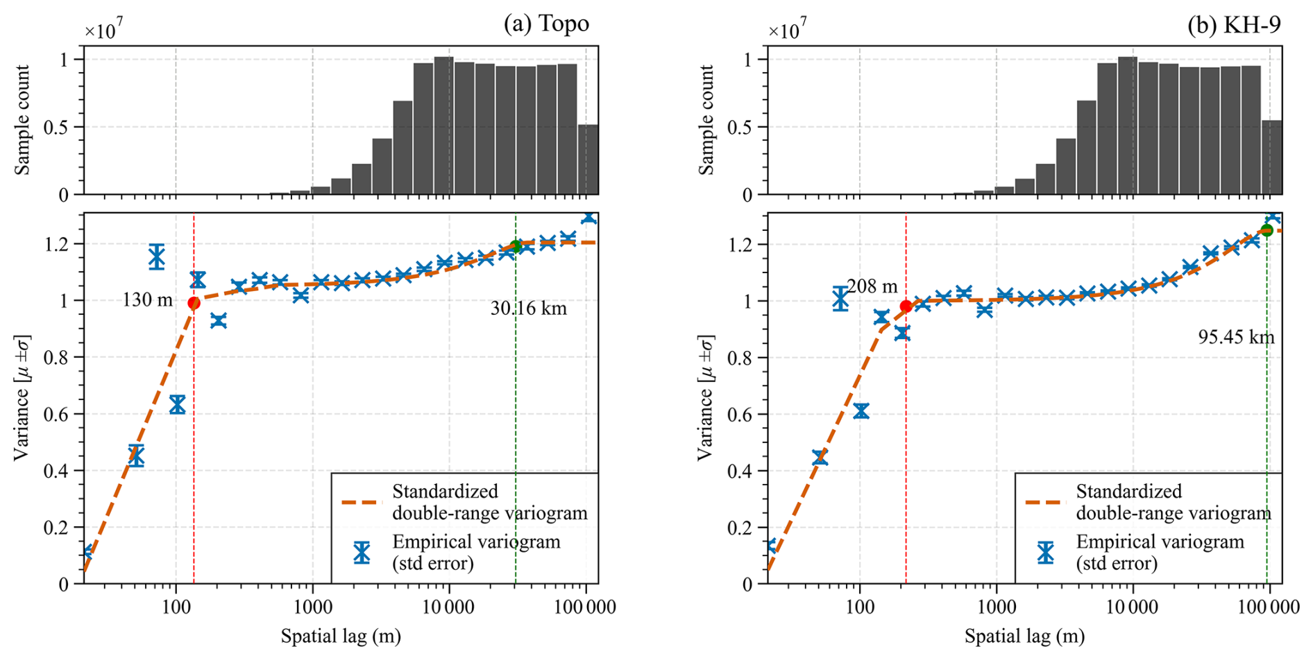
Figure 8 Spatial autocorrelation characteristics of the Topo DEM (a) and the KH-9 DEM (b). For both data, a Gaussian model was used to fit the short-range variogram, and a spherical model was used for the long-range variogram.

We therefore evaluated the precision of the KH-9 and Topo DEMs by examining two aspects: heteroscedasticity and spatial autocorrelation. The analysis revealed a pronounced dependence of errors on both slope and curvature for both the topographic map and the KH-9 data. In areas with a maximum absolute curvature of less than $\mathrm{1}/\mathrm{100}$ m⁻¹ and a slope of less than 20°, the NMAD of the off-glacier region for the Topo DEM was 4.7 m, while the KH-9 DEM exhibited a significantly higher NMAD of 13.4 m (Fig. 7). Although both DEMs displayed larger errors in high-altitude, steep-slope regions, the errors associated with the KH-9 DEM were substantially greater, which aligns with the previous statistical findings. This suggests that the Topo DEM exhibits lower errors stemming from elevation heteroscedasticity. The spatial autocorrelation evident in Fig. 8 was further quantified by analyzing both short-range and long-range correlations. The results indicated that the Topo DEM consistently displayed lower values for both types of autocorrelation compared to the KH-9 DEM. Notably, the long-range autocorrelation – which has a greater influence on the uncertainty of glacier surface elevation changes – exceeded 30 km for both DEMs. The estimation of long-range spatial correlations for the KH-9 DEM is consistent with that of Dehecq et al. (2020). This limited the number of independent elevation difference pixels, ultimately increasing the uncertainty in the final estimates of glacier surface elevation change according to Eq. (6). The observed issues with the Topo DEM likely stem from the scarcity of national elevation control points in border regions, leading to a comparatively lower DEM accuracy.

In addition, the concordance observed between Topo- and ICESat-derived elevation differences further corroborates the applicability of the Topo DEM product at low elevations (see Sect. S1 in the Supplement). These findings suggest that the precision of glacier surface elevation change results generated from topographic maps is, at minimum, on par with the established accuracy of glacier change products derived from KH-9 data. However, it is imperative to acknowledge the limitations associated with Topo map products. When employing these data for specific applications, it is essential to consult the uncertainty assessments provided within our dataset for each individual glacier or grid cell.

4.2 Uncertainties arising from topographic map production processes

Most of the uncertainties in Topo DEMs stem from the processes involved in generating and performing interpolation (Junfeng et al., 2018). Achieving high map accuracy requires adherence to standard contour intervals (see Table S2). However, this is increasingly difficult in steep terrains because dense lines cannot be drawn within the limited space (Fig. S7). This, coupled with the strategies in cartographic generalization of diverse land cover, leads to uncertainties in the contours.

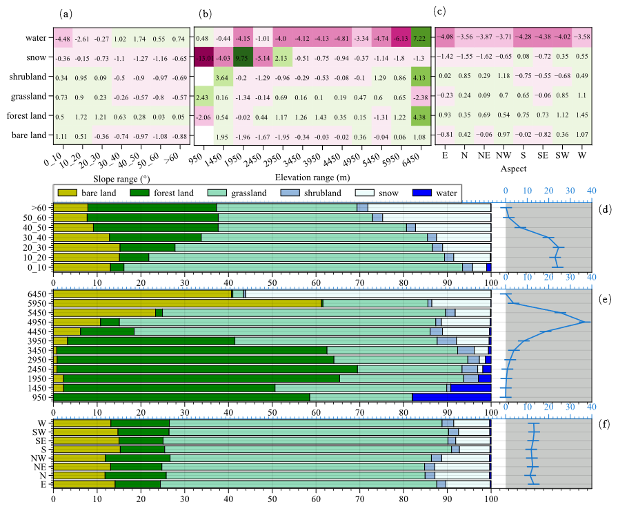
Figure 9 Elevation differences in off-glacier regions by slope (a), elevation zone (b), and aspect (c) across different land covers. The land cover ratios are displayed in panels (d–f). Blue lines within gray shadows in panels (d–f) represent the total area proportions in a specific classification. The units in panel (a–c) are meters, while in panel (d–f) they are percentages.

To assess the uncertainties, we analyzed off-glacier regions categorized into six land cover types (Fig. 9). Grassland and bare land exhibited minimal uncertainties (∼ 0.31 and −0.44 m, respectively) due to their minimal elevation variations compared to forested areas. Additionally, their larger and more continuous high-altitude patches facilitated denser elevation point placement. Notably, a positive difference (∼ 1.21 m) arose from neglecting tree height in contour generation. Snow cover regions displayed increasing uncertainty with elevation and slope. Despite comprising approximately 8 % of the whole statistical region, its uncertainty mirrored that of the glacial area due to similar distributions. High contour line density is crucial for accurate mapping in steep high-altitude terrains. However, map-maker limitations and national standards specifying wider spacing in high-altitude regions (Fig. S7 and Table S2) lead to significant uncertainties in snow-covered areas. Low-altitude snow cover variations have a minimal impact on long-term glacier elevation changes. Due to the dispersed distributions of water bodies and the expansion of the lakes during the study period, the elevation differences in the water bodies are inaccurate. Uncertainty in orientation remained consistent across the land cover types (Fig. 9c). Overall, uncertainties increase with slope, likely due to past compilation limitations and poorer technical capabilities in representing steep terrains. This slope-dependent accuracy issue is common to other DEM products (SRTM DEM, ASTAR GDEM, and SPOT5-based DEM) (Kocak et al., 2004; Rodríguez et al., 2006). Consequently, geodetic-based ice mass change estimates might have significant uncertainties in steep terrains, particularly glacier accumulation zones.

Another uncertainty is the interpolation process in generating DEMs from contours. Interpolation methods have a certain amount of influence on accuracy, and the natural-neighbor method displays relatively high accuracy (Habib, 2021). However, almost every interpolation method faces challenges in high-altitude regions since the interpolation leads to a smooth surface structure, especially on steep slopes. While meshing techniques have demonstrated the ability to generate refined topographical structures closely aligned with actual terrain (Pieczonka et al., 2011), their application in generating Topo DEMs is constrained by the limited density of elevation points available on topographical maps (8–15 per 100 mm² in alpine regions on topographical maps according to GB/T 12343.1-2008). Topographical maps have been successfully employed in numerous studies investigating glacier dynamics, despite these limitations (e.g., Ye et al., 2017; Junfeng et al., 2018; Wu et al., 2018).

Nevertheless, we made a comprehensive quantitative assessment of these uncertainties by analyzing the elevation difference characteristics in off-glacier regions (refer to Sect. 3.1). In contrast to previous studies (e.g., Ye et al., 2017; Wu et al., 2018), our approach quantifies the long-range spatial autocorrelation errors potentially arising from the topographic map generation process rather than solely focusing on short-range spatial autocorrelation errors introduced by interpolation. This more comprehensive error assessment strengthens the robustness and applicability of our dataset.

4.3 Comparison of glacier mass changes derived from Topo and KH-9

To date, there have been few observations of mass changes prior to 2000 in the whole ETPR. A few regional studies based on topographical maps (e.g., Ye et al., 2015) offer some insights, but their coverage is limited. Conversely, studies utilizing KH-9 data (e.g., Maurer et al., 2019; Bhattacharya et al., 2021) with sufficient coverage can serve as an independent source for comparison and validation of mass balances derived from the Topo DEM. We therefore compared our dataset with the KH-9 assessments, particularly the works of Zhou et al. (2022) and Bhattacharya et al. (2021). Focusing on the Himalayas, previous studies reported mass changes ranging from −0.17 to −0.32 $\mathrm{m}\mathrm{w}.\mathrm{e}.{\mathrm{yr}}^{-\mathrm{1}}$ (Table S3), which was generally consistent with our findings. However, some discrepancies emerged at the basin or regional scale. For example, for the Yigong Zangbo and Parlung Zangbo (mainly included in the Salween and the Brahmaputra), mass balances of −0.11 ± 0.14 and −0.19 ± 0.14 $\mathrm{m}\mathrm{w}.\mathrm{e}.{\mathrm{yr}}^{-\mathrm{1}}$, respectively, were reported by Zhou et al. (2018). These values diverge slightly from our Topo-derived estimate of less than −0.24 ± 0.12 $\mathrm{m}\mathrm{w}.\mathrm{e}.{\mathrm{yr}}^{-\mathrm{1}}$, potentially due to incomplete data used in the previous study. This difference highlights the significance of data sources and methodologies for the estimation of mass balances. As other datasets were unavailable, we used the results of Bhattacharya et al. (2021) for further analysis.

Our total ETPR-wide mass balance (−0.30 $\mathrm{m}\mathrm{w}.\mathrm{e}.{\mathrm{yr}}^{-\mathrm{1}}$) is slightly higher than the value (−0.22 $\mathrm{m}\mathrm{w}.\mathrm{e}.{\mathrm{yr}}^{-\mathrm{1}}$) reported by Bhattacharya et al. (2021). This difference could stem from different sources. First, discrepancies in the methodologies used to generate DEMs from optical imagery might contribute. Second, a minor inconsistency exists in the reference periods for calculating elevation changes. The acquisition dates for KH-9 images primarily range from 1964 to 1976, while topographical maps were acquired from 1957 to 1983. While we accounted for annual differences, slight variations due to these time frames might persist. However, the most important factor likely influencing the difference is the coverage of the compared results. As Wang et al. (2019) highlight, the glacier mass balance exhibits significant spatial heterogeneity across large regions due to variations in topography and meteorological conditions. This heterogeneity can even be observed within specific mountain ranges. Consequently, it is challenging to determine whether regional mass balance estimates, based on a limited area, accurately represent the mass budget of the entire ETPR. Therefore, rather than focusing solely on the overall difference, a more meaningful analysis would involve comparing mass balance estimates within specific regions where both KH-9 and Topo DEM data overlap.

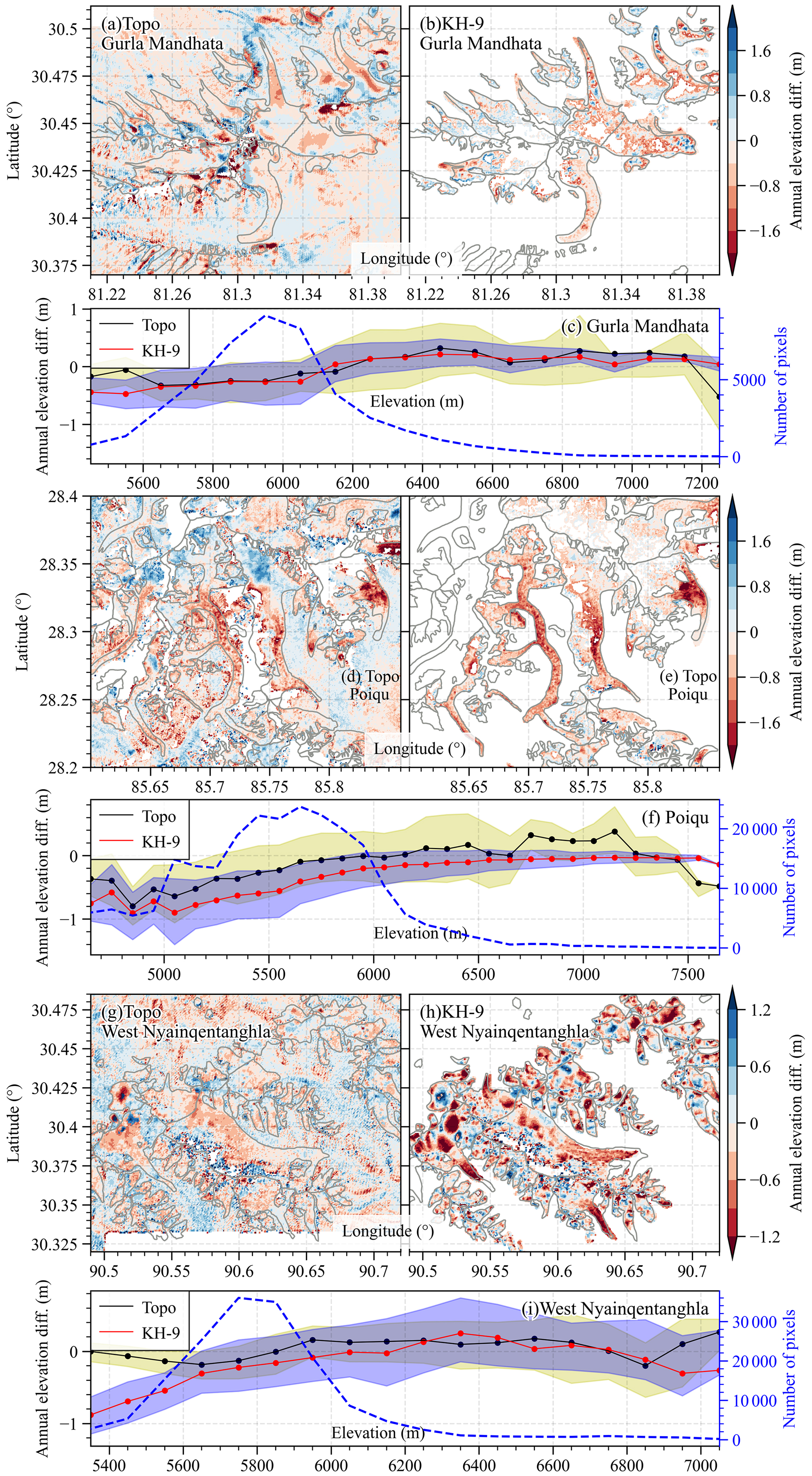
Figure 10 Annual elevation differences derived from Topo and KH-9. The distribution of elevation differences along altitude is presented in panels (c), (f), and (i). The light shadows in panels (c), (f), and (i) represent the 50 % CI.

Table 4 Glacier mass balances ($\mathrm{m}\mathrm{w}.\mathrm{e}.{\mathrm{yr}}^{-\mathrm{1}}$) derived from the KH-9 and Topo DEMs in selected regions. The source of the results is derived from KH-9 panoramic camera data (Bhattacharya et al., 2021).

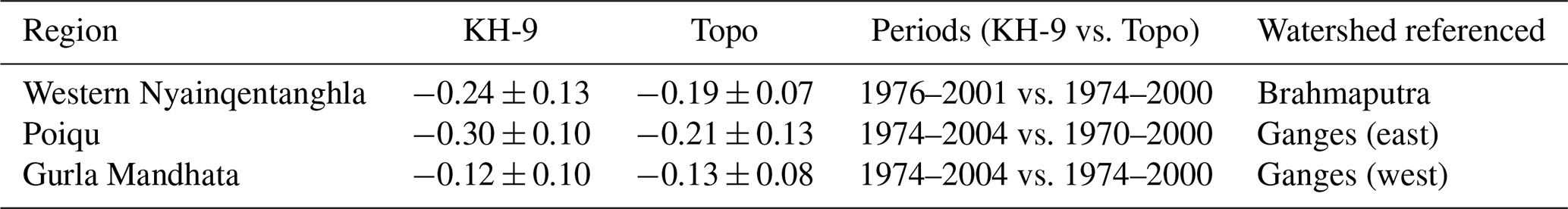
Due to the availability of the KH-9 elevation difference, only two subregions in the Ganges basin and one subregion in the Brahmaputra basin were selected for regional comparisons. Notably, both results revealed similar heterogeneity in mass changes, with values increasing from east (Western Nyainqentanghla) to west (Gurla Mandhata). In the Western Nyainqentanghla region, our estimate (−0.13 ± 0.06 $\mathrm{m}\mathrm{w}.\mathrm{e}.{\mathrm{yr}}^{-\mathrm{1}}$) was less negative than the estimate based on KH-9 (−0.24 ± 0.12 $\mathrm{m}\mathrm{w}.\mathrm{e}.{\mathrm{yr}}^{-\mathrm{1}}$) during 1976–2001 (Bhattacharya et al., 2021). This could be attributed to the slightly different acquisition times. By comparing the elevation differences in the subregion (Langtang) of the Poiqu region (Fig. 10d and e, Table 4), we conclude that the difference in the data coverage and glacier boundary is also a cause of less negative mass change in our results. The more negative mass balance derived from the Topo DEM for the Gurla Mandhata region likely arises from data-filling strategies. The filled region (6250–6900 m) in our data exhibits a near-zero mass budget, while the corresponding area in the KH-9 data shows a gap (Fig. 10a and b). In order to clarify this phenomenon and promote more flexible applications of our dataset, we also provide the elevation difference data with no gap-filling.

For all of the compared regions, the annual elevation differences display similar patterns across the altitude between KH-9 and Topo, and a notable discrepancy emerges at the glacier tongue (Fig. 10c, f, and i). Here, KH-9 data consistently yield more negative elevation changes (greater thinning rates) compared to Topo DEM data, with differences ranging from 0.2 to 0.5 m yr⁻¹. This discrepancy is particularly pronounced in the Nyainqentanglha region. It is important to note that our analysis excludes a small portion of the glacier tongue where the largest surface thinning is observed. Despite this exclusion, our Topo-based results exhibit relatively low variability (an NMAD of 5.61 m) across elevations. This stands in contrast to the more pronounced variation seen in the elevation change distribution derived from the KH-9 data. These observations suggest potential uncertainties associated with the production of either Topo DEMs or KH-9 DEMs.

To further confirm that our data can give a comprehensive and effective expression of the whole study region, we conducted a comparison with the results post-2000 (e.g., Brun et al., 2017; Shean et al., 2020; Hugonnet et al., 2021), which have more extensive coverage. All of the studies, including our Topo-based analysis, identified the Salween source area as a central zone of significant mass loss (Table S4). However, the results derived from KH-9 indicated that the eastern–central Himalayas were the region with the largest glacier surface thinning. Under the assumption of relatively consistent climatic variability across basins, the spatial heterogeneity of mass balance at the basin scale would likely remain the same. By comparison, the Topo-derived mass balance was found to exhibit the same spatial heterogeneity with the average of the estimates of Brun et al. (2017) and Shean et al. (2020) (excluding the Yellow and Irrawaddy basins due to small glacier cover). This highlights how dataset convergence can influence our understanding of glacier mass balance heterogeneity for a large region.

5 Data availability

The ETPR glacier surface mass change database is distributed under the Creative Commons Attribution 4.0 License. The data can be downloaded from the data repository of the National Tibetan Plateau/Third Pole Environment Data Center at https://doi.org/10.11888/Cryos.tpdc.301236 (Liu et al., 2024).

6 Code availability

The code used for processing and analyzing all of the data is available at https://doi.org/10.5281/zenodo.15357957 (Zhu, 2025). The implementation of key scripts for error assessment is primarily based on the xDEM Python package (https://doi.org/10.5281/zenodo.11204531, Hugonnet et al., 2024).

7 Conclusions

This study presents a near-complete glacier mass change dataset for the pre-2000 period, encompassing approximately 70 % of the study area's total glacier extent. This comprehensive inventory provides valuable insights into the spatial heterogeneity of glacier changes across the region. The gridded products, in combination with the published results, provide a nearly 5-decade record of mass balances to support parameter calibration in hydrological simulation and energy balance simulation and to evaluate the contribution of mountain glacier loss to sea level.

The overall mass balance in the ETPR from the 1970s to 2000 is −0.30 ± 0.12 $\mathrm{m}\mathrm{w}.\mathrm{e}.{\mathrm{yr}}^{-\mathrm{1}}$. Small glaciers experienced the most negative mass change. The mass balance exhibits a pronounced latitudinal gradient, showing that regions farther south experience greater mass loss.

Compared to prior Topo map products, our datasets offer a more comprehensive analysis of glacier mass balance uncertainties by incorporating data from stable areas, addressing uncertainties from heteroscedasticity of elevation measurements, and considering the previously neglected uncertainties of long-range correlation in elevation measurements. This in-depth analysis pinpoints the generation process of elevation contours and the increasing uncertainty with steeper slopes as the main drivers of mass budget uncertainty. These findings highlight the importance of meticulously evaluating and mitigating these uncertainty sources when interpreting glacier mass balance estimates, especially in areas with challenging topography.

Systematic comparisons between Topo- and KH-9-derived results indicate that our product achieves an accuracy level comparable to, if not exceeding, that of KH-9. However, both Topo- and KH-9-based results have low reliability at high altitudes. Despite this, the overall mass balance estimates derived from Topo DEM data remain consistent with those obtained using KH-9. Nevertheless, some regional discrepancies in mass balance knowledge are evident when compared to KH-9 findings. These discrepancies can be attributed to two primary factors. Firstly, the inherent limitations in the spatial coverage of KH-9 data potentially restrict the comprehensiveness of the analysis in certain regions. Secondly, the specific methodological approaches employed during the generation of each DEM may introduce systematic biases that contribute to the observed variations.