Advancing geodynamic research in Antarctica: reprocessing GNSS data to infer consistent coordinate time series (GIANT-REGAIN)

For nearly 3 decades, geodetic Global Navigation Satellite System (GNSS) measurements in Antarctica have provided direct observations of bedrock displacement, which is linked to various geodynamic processes, including plate motion, post-seismic deformation, and glacial isostatic adjustment (GIA). Previous geodynamic studies in Antarctica, especially those pertaining to GIA, have been constrained by the limited availability of GNSS data. This is due to the fact that GNSS data are collected by a wide range of institutions and network operators, with the raw observational data either not publicly available or scattered across various repositories. Further, the metadata necessary for rigorous data processing have often not been available or reliable. Consequently, the potential of GNSS observations for geodynamic studies in Antarctica has not been fully exploited yet. Here, we present consistently processed coordinate time series for GNSS sites in Antarctica and the sub-Antarctic region for the time span from 1995 to 2021. The data set is composed of 286 continuous and episodic sites, with 258 sites having a time span longer than 3 years. The coordinate time series were obtained from a combination of four independent processing solutions using different GNSS software and products, allowing the identification of inconsistencies in individual solutions. From these, we infer a reliable and robust combined solution. A key issue was the thorough reassessment of station metadata to minimise artefacts and biases in the coordinate time series. The resulting data set provides coordinate time series with unprecedented spatiotemporal coverage, promising significant advancements in future geodynamic studies in Antarctica. The data set is freely available at https://doi.org/10.1594/PANGAEA.967515 (Buchta et al., 2024a).

1 Introduction

The deformation of the solid Earth is caused by a multitude of geodynamic processes that occur on different temporal and spatial scales. Measurements using the geodetic Global Navigation Satellite System (GNSS) on bedrock were first conducted in Antarctica in the mid-1990s. These have proven to be highly effective for determining bedrock displacement to quantify and characterise underlying geodynamic processes, such as the determination of plate motion (Bouin and Vigny, 2000; Dietrich et al., 2001, 2004; Savchyn et al., 2023), the assessment of post-seismic deformation (King and Santamaría-Gómez, 2016; Nield et al., 2023), the validation of ocean tide models (King et al., 2005), or studies of local deformation due to volcanism (Grapenthin et al., 2022). In terms of current research, deformation processes originating from the interaction of the solid Earth with the Antarctic Ice Sheet (AIS), which manifest themselves predominantly as vertical bedrock displacement, are of greatest importance. Here, traditionally a distinction is made between (1) the instantaneous, elastic response of the solid Earth to contemporary ice-mass changes caused by dynamic ice-mass loss and variations in the surface mass balance (SMB) (Koulali et al., 2022) and (2) the viscoelastic response to past ice–ocean loading changes – known as glacial isostatic adjustment (GIA).

The determination of GIA plays a prominent role in current climate research (King et al., 2010). Gravity observations from the Gravity Recovery and Climate Experiment (GRACE) and Gravity Recovery and Climate Experiment Follow-on (GRACE-FO) missions are used to determine the mass change of the AIS (King et al., 2012; Groh and Horwath, 2021; Otosaka et al., 2023) and, consequently, its contribution to current sea-level rise. Here, the standard procedure involves a reduction in the GRACE observations by the mass effect of GIA, to isolate the mass signals of present-day ice-mass change. However, both inverse and empirical GIA models differ significantly in their spatial pattern and amplitude (Martín-Español et al., 2016; Whitehouse, 2018), making the GIA correction the largest contributor to the uncertainty in the estimated ice-mass changes from GRACE and GRACE-FO observations (Otosaka et al., 2023).

A multitude of studies employed GNSS observations to ascertain GIA-induced vertical rates on a regional (Bevis et al., 2009; Argus et al., 2011; Scheinert et al., 2006; Zanutta et al., 2017; Hattori et al., 2021; King et al., 2022) and continental scale (Thomas et al., 2011; Argus et al., 2014; Rülke et al., 2015; Liu et al., 2018; Li et al., 2022). Regional studies can make an important contribution to highlight local or regional deficiencies in GIA models. For example, King et al. (2022) utilised GNSS observations to report on widespread rates of subsidence in the East Antarctic region between 77 and 120° E, after correcting for SMB-induced variations and common mode errors, which are not included in any GIA forward model. King et al. (2022) suggested shortcomings in the assumed ice-load history, postulating a Late Holocene readvance of the ice sheet in the region west of Denman Glacier. In West Antarctica, the Amundsen Sea region exhibits particularly high uplift rates of up to 60 mm yr⁻¹ with steep spatial gradients (Groh et al., 2012; Busch et al., 2017; Barletta et al., 2018), which are not reflected in most GIA models. Barletta et al. (2018) used GNSS observations to derive a regional GIA model, obtaining a low viscosity of the upper mantle ranging from just 4×10¹⁸ to 2.5×10¹⁹ Pa s. The derived upper-mantle viscosity is 2–3 orders of magnitude lower than that typically used for GIA models covering whole of Antarctica, resulting in a significantly reduced GIA response time to ice-mass changes of just decades to centuries. A similarly low viscosity mantle was identified using GNSS and models in the northern Antarctic Peninsula (Nield et al., 2014; Samrat et al., 2020, 2021).

Given the diversity in spatiotemporal patterns inherent in various geodynamical processes, the requirements for a comprehensive data set inferred from GNSS time series to observe these processes are manifold:

• To accurately assess the GIA effect on a continental scale as well as signals with smaller spatial wavelengths, it is essential to provide a data set with the best possible spatial coverage with respect to both extent and resolution.

• To correctly resolve non-linear geodynamic processes (Nield et al., 2014; Liu et al., 2018; Koulali et al., 2022; Nield et al., 2023), it is necessary to produce time series with a sufficient temporal resolution, typically a daily resolution. To derive accurate secular rates or detect changes in rates, one aims to maximise the time span of the GNSS time series.

• To allow for an assessment of GIA models on the accuracy level of 1 mm yr⁻¹, highly consistent and accurate data are required. As demonstrated by Martín-Español et al. (2016), a GIA model error of 1 mm yr⁻¹ integrated over the area of East Antarctica translates into a mass effect of 45 Gt yr⁻¹, which is equivalent to the magnitude of the signal itself.

Presently, no data set can be considered to fulfil the above points to the best possible extent. The reasons for this are manifold. While the observation data are freely accessible for some large GNSS networks, e.g. POLENET (the Polar Earth Observing Network; Wilson et al., 2019) or the IGS (International GNSS Service) network (Johnston et al., 2017; Vardić et al., 2022), the observation data of smaller networks or individual stations are either scattered over various repositories or are not freely accessible. In particular, historic campaign/episodic measurements are often unavailable, even though they can greatly enhance the spatial coverage of a data set. Metadata, i.e. information on the site set-up, are essential to determine consistent coordinate time series but are often insufficiently documented, especially for past (mostly episodic) sites and measurement campaigns, leading to the potential misinterpretation of derived coordinate trajectories. Coordinate time series data sets produced with a high degree of automation, such as those provided by the Nevada Geodetic Laboratory (NGL; Blewitt et al., 2018), rely on metadata stored in the observational RINEX (Receiver Independent Exchange Format) files, which can be prone to errors. The combination of coordinate time series or displacement rates derived from heterogeneous or independent studies (e.g. combining regional and continent-wide studies) is not advisable, as different studies rely on differing processing conventions, like the adopted reference frame or specific geophysical reductions, resulting in an inconsistent data set. Before realising a data combination of this kind, a consistent processing of all observation data is mandatory.

To exploit the full potential of GNSS observations in Antarctica, the SCAR-endorsed (where SCAR denotes the Scientific Committee on Antarctic Research) GIANT-REGAIN (Geodynamics In ANTarctica based on REprocessing GNSS dAta Initiative) project was initiated and aimed to acquire and consistently process all available GNSS recordings on bedrock in Antarctica for the period from 1995 to 2021. Here, we present the results of the GIANT-REGAIN project, providing coordinate time series as the main product. We report on the acquisition of observational data that originate from more than 20 different networks and institutions, including freely accessible data and data from past measurement campaigns. We could especially obtain observational data from previously unpublished GNSS sites. The relevant site metadata, which are indispensable for the correct assignment of the hardware set-up, were re-evaluated and, if necessary, corrected.

The observational data were processed by four contributing analysis centres (ACs), namely, the Dresden University of Technology (TUD), the University of Tasmania (UTAS), The Ohio State University (OSU), and Newcastle University (NEWC). The inclusion of multiple independent ACs allows us to evaluate the processing noise and, specifically, to undertake the following:

• validate and detect inconsistencies in the individual solutions,

• assess systematic differences (biases) in the resulting coordinate time series on different temporal scales, and

• assess and compare noise characteristics of the individual coordinate time series.

Subsequently, the individual coordinate time series were used to form a combined final data set. This is beneficial, as not all centres produced solutions for every site and day with valid observations. Thus, the combination enables us to maximise the spatiotemporal coverage compared to the individual solutions while also preserving the noise level of the individual solutions. The final data set comprises coordinate time series for 286 GPS sites. Therefore, this data set provides the most comprehensive spatiotemporal coverage ever for Antarctica. Equipment changes can alter the trajectory of GPS coordinate time series. We rigorously revised the metadata records for all sites within our data set to ensure the correct interpretation of the coordinate time series with respect to the geodynamic processes. Clear and accurate metadata records also allow for the best possible inter-centre consistency and provide a reliable foundation for future reprocessing. Furthermore, GPS sites with a missing or incomprehensible metadata record as well as sites showing clear monument instability in their coordinate trajectory were not considered for the final product.

We compared our resulting coordinate time series to the latest data set by the Nevada Geodetic Laboratory (NGL; Blewitt et al., 2018), which has provided, until present, the most extensive record of processed GNSS coordinate time series in Antarctica. This is a convenient and widely used open-access data set that has been employed in recent studies (Li et al., 2022; Savchyn et al., 2023). We assess differences between the data sets on secular timescales (linear rates) and demonstrate the impact of the updated GIANT-REGAIN metadata information on adopted antenna heights.

2 Data acquisition

2.1 Observational data

The primary objective of this study is to analyse and provide a data set that includes all GNSS observations on bedrock for the period from January 1995 to December 2021. Before going into detail, we want to briefly emphasise the usage of the terms GNSS and GPS. The first GNSS deployments tracked only GPS satellites. Many of these sites have since been upgraded with receivers capable of tracking multi-GNSS constellations, making it more correct to refer to these specific sites as GNSS stations. However, the processing strategies applied in this study were limited to GPS observations, resulting in coordinate time series based on GPS-only observations. Therefore, we use the terms GPS stations and GPS coordinate time series throughout the rest of this paper. The required GPS observational data, in the form of raw binary files or the RINEX format, were (to the extent possible) obtained from publicly accessible repositories. The Geodetic Facility for the Advancement of Geoscience (GAGE) manages the observational data and metadata for POLENET-associated stations and makes them publicly available. Observational data for GPS sites contributing to the global IGS network are made publicly available via multiple repositories (e.g. the CDDIS – Crustal Dynamics Data Information System). The observational data from smaller networks or past measurement campaigns are included in GAGE, scattered over smaller data repositories, or not publicly available at all (see Table S1 in the Supplement for the complete list of DOIs for the observational data).

Following a first call for data contribution by the initiators of the GIANT-REGAIN project in 2016, more than 20 station operators and national Antarctic research programmes supported the provision of GPS data for this project. This included stations with already processed and published time series as well as GPS stations with so far unpublished coordinate time series. Figure 1 provides an overview of the spatial distribution of the GPS sites and their associated networks. To observe geodynamic processes related to solid-Earth deformation, the measurements need to refer to specifically marked points in the bedrock. With only 0.18 % of the Antarctic continent consisting of ice-free bedrock (Burton-Johnson et al., 2016), suitable locations for GPS sites are limited to the coastal regions and mountain ranges.

Antarctic GPS sites have been occupied in two ways: in a campaign-style manner with episodic measurements (eGPS) or as continuously operating installations (cGPS). Episodic measurements are realised using the antenna on a fixed marker in the bedrock, with equipment removed at the end of each campaign and reinstalled after an interval typically of a year or more. Occupations typically last a few days to a few weeks.

The first cGPS sites were set up near research stations in the early and mid-1990s. These sites contribute to the global IGS network (Johnston et al., 2017) and provide the longest and most complete observation record within this study. The IGS sites were set up at staffed Antarctic stations, namely, Casey (CAS1), Mawson (MAW1), Dumont d'Urville (DUM1), Davis (DAV1), McMurdo (MCM4), and Syowa (SYOG). Later, additional sites were incorporated into the IGS network, such as Scott Base (SCTB), Mount Coates (COTE), O'Higgins (OHI2 and OHI3), Arrival Heights, McMurdo (ARHT), Rothera (ROTH), and Palmer Station (PALM), while other sites lost their IGS status (e.g. Vesleskarvet – VESL) or were decommissioned (PALV and OHIG).

Starting in 1995, several projects were launched to establish additional regional and local GPS networks. The SCAR Epoch Crustal Movement Campaigns from 1995 to 1999 focused on the regions of the Antarctic Peninsula and Dronning Maud Land and comprised coordinated episodic measurements with contributions and support from several national polar programmes (Dietrich et al., 2001, 2004). The TAMDEF (Transantarctic Mountains Deformation) project, with its first observations in 1996, established a GPS network covering large parts of the Transantarctic Mountains, consisting of 25 episodic, 6 quasi-continuous, and 2 continuous sites (Raymond et al., 2004; Vázquez Becerra, 2009). The first sites of the VLNDEF (Victoria Land Network for DEFormation Control) network were installed during field campaigns in 1999–2000 and 2000–2001 (Zanutta et al., 2017, 2018), with 28 sites in the final configuration. The WAGN (West Antarctic GPS Network) was operated between 2001 and 2006 and covered yet unobserved regions of West Antarctica (Bevis et al., 2009). A small GPS array of episodic sites was installed in the region of western Marie Byrd Land over 1999–2002 (Donnellan and Luyendyk, 2004) and around the Amery Ice Shelf in East Antarctica Tregoning et al. (1999, 2000).

The harsh Antarctic conditions, such as low temperatures and the polar night, introduce particular technological and logistical challenges to the establishment and maintenance of GPS stations. Establishing a continuous and resilient energy supply has posed significant problems. Moreover, undertaking maintenance work presents a significant logistical challenge, and data transfer must be accomplished either remotely or through manual collection. An essential increase in the spatial coverage of remote cGPS was achieved following the International Polar Year (IPY) from 2007 to 2009 (see Fig. 1b). The POLENET-embedded network ANET formed the nucleus of the initiative. The ANET network extends from Victoria Land to the Amundsen Sea embayment and Filchner–Ronne Ice Shelf, covering major parts of West Antarctica. Within the POLENET initiative, some of the previous eGPS sites of the WAGN, TAMDEF, and Marie Byrd Land network were reoccupied and upgraded to cGPS sites. International partners contributed to the ANET network. Three sites of the VLNDEF (VL01, VL12, and VL30) network were upgraded to cGPS sites and included in the POLENET network in the 2014–2015 season (Zanutta et al., 2017). The POLENET–UKANET network of cGPS sites covers large parts of the Antarctic Peninsula and the surroundings of the Filchner–Ronne Ice Shelf (Whitehouse et al., 2020). It includes sites of the LARISSA (LARsen Ice Shelf System, Antarctica) network, consisting of six cGPS sites (installed in 2008 and 2010) covering the northern part of the Antarctic Peninsula (Nield et al., 2014), and the CAPGIA (Constraints on Antarctic Peninsula GIA) network (King et al., 2013; Wolstencroft et al., 2015), installed in the 2009–2010 Antarctic summer season and consisting of nine cGPS sites. In addition to these large-scale networks, networks with a smaller spatial extent exist that are operated by various institutions. TUD continues to operate eGPS stations in the area of the Antarctic Peninsula, in Dronning Maud Land, and in the Amundsen Sea embayment, which in part represent the continuation of the initial measurements of the SCAR Epoch Crustal Movement Campaigns (Rülke et al., 2015; Scheinert et al., 2023). The Japanese Antarctic Research Expedition (JARE) operates a local network at the Lützow-Holm Bay (69–70° S, 37–40° E) (Hattori et al., 2021). In addition to the IGS station SYOG, episodic measurements were initially carried out and later partially upgraded to cGPS stations (the observational data from the cGPS stations were not available for this study). King et al. (2022) installed a network of six cGPS sites, providing observations for the so far barely covered coastal area of East Antarctica between Davis and Casey stations (70–120° E). Observational data from five sites were available for this study. Several sites are not affiliated with larger networks and are often co-located with research stations (e.g. ABOA (Andrei et al., 2018), NONS, SVEA, KOH2, VESL, and LXAA). These sites can contribute significantly to an increased spatial coverage, especially in East Antarctica where the coverage is otherwise very sparse. The number of daily observations within Antarctica increased steadily from 1995 (Fig. 1b) with a significant increase in 2008 with the initiation of the POLENET project. The peak number of daily site observations (100) was reached in 2016 and has remained somewhat steady since. However, the observation count decreased in 2020, partly due to the COVID pandemic, when maintenance work and manual data retrieval were not possible for some sites.

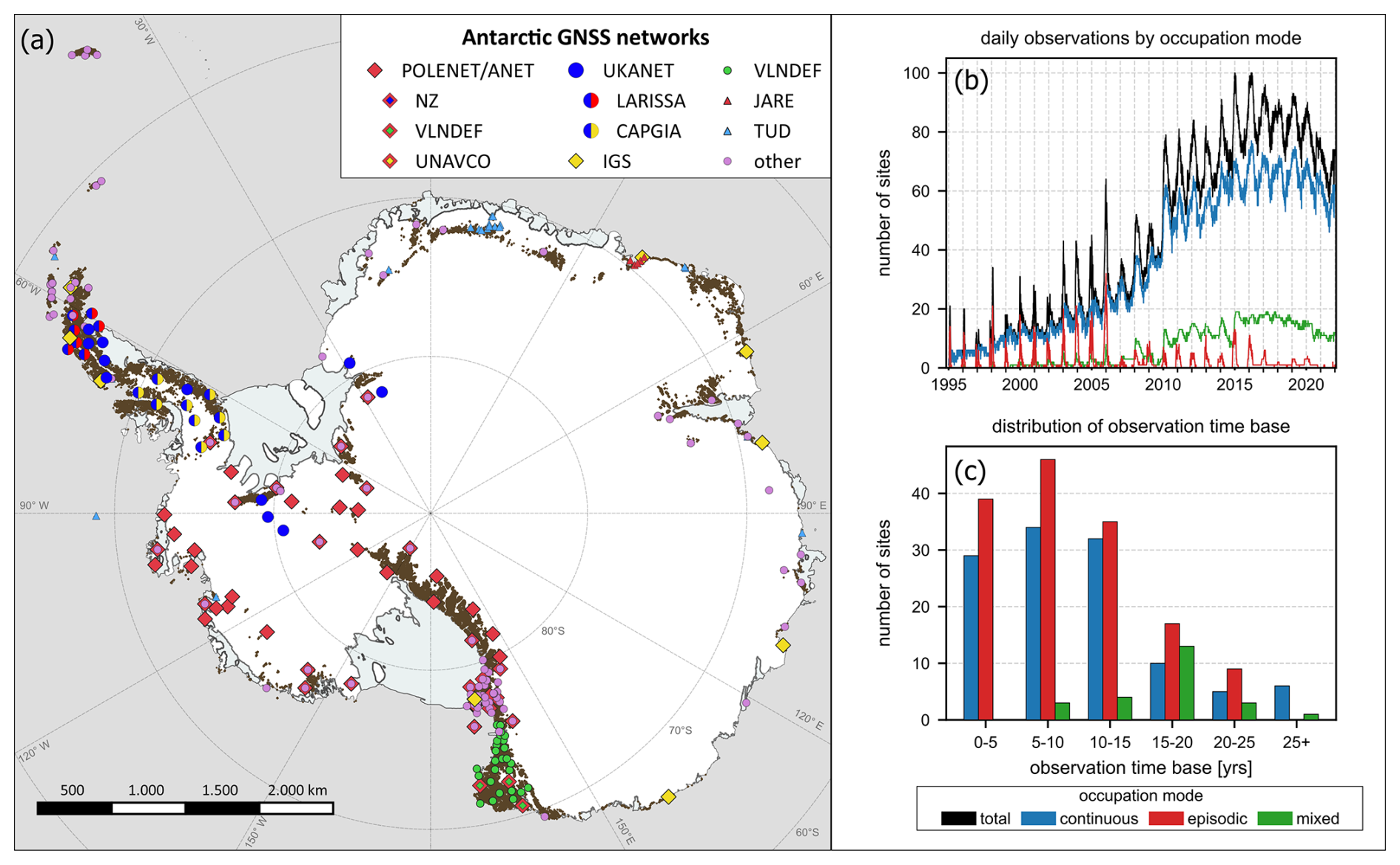
Figure 1 (a) Spatial distribution of GNSS sites on bedrock and selected network affiliations. Bedrock outcrops are indicated in brown (Burton-Johnson et al., 2016). The association of a GNSS site with a network is generally not unique, as sites can be attributed to multiple networks at a time or former networks can have been integrated in newly established ones. The temporal development of the observation data, shown in panel (b), reveals a steady increase in the number of data up to 2016. Following the International Polar Year (IPY) in 2008–2009, a strong increase in observations of cGPS sites in particular can be seen, while the number of eGPS observations decreased significantly. The “mixed” occupation type refers to sites that were initially installed as episodic sites and later upgraded to continuously operating installations. The observation time base, as shown in panel (c), results from the difference between the first and last observation and, therefore, does not contain any information about the temporal coverage within the observation period.

2.2 Metadata

Correct metadata are essential to determine consistent time series from GPS. In the context of GPS data processing, the metadata contain information about the hardware set-up. Incorrect information can lead to biased, more noisy time series and, subsequently, to errors in derived deterministic parameters, such as linear trends. Correct metadata are of utmost importance for eGPS (Scheinert et al., 2023), as errors in the metadata (e.g. antenna heights) can bias measurement campaigns and are not necessarily detectable by the analysis of the coordinate trajectories (depending on the number of measurements).

Basic information is usually provided in the RINEX header section and includes, among others, information about the installed antenna (type and serial number), receiver (type, serial number, and firmware version), and antenna eccentricities. For past sites, the RINEX header often contains incomplete or even false information. For this study, we confirmed or corrected the metadata information, using metadata logs, observation protocols, images of the GPS stations (with a focus on the antenna set-up), published metadata information, or personal communication with site operators.

To ensure the reproducibility of the processing and to enable possible future reprocessing, the metadata are provided in the established and comprehensive format of the station log files (https://files.igs.org/pub/station/general/sitelog_instr.txt, last access: 15 July 2024) of the IGS (Buchta et al., 2024d).

Multiple studies (Argus et al., 2014; Konfal et al., 2016; Koulali and Clarke, 2020) have reported on the effect of snow intrusion into the GPS antenna radomes through drainage holes in the ground plates for a subset of ANET and UKANET cGPS sites, leading to offsets and quasi-periodic (annual) signals in the coordinate time series. As a countermeasure, the drainage holes were initially closed with tape and later sealed with permanent plugs. A comprehensive list of efforts regrading the sealing of drainage holes was provided for this study (David Saddler, OSU, personal communication, 11 October 2023). Understanding the sealing efforts is crucial to accurately interpret the coordinate time series, as this can significantly alter the coordinate trajectory. The antenna sealing efforts are listed within the auxiliary data published in conjunction with the coordinate time series (Buchta et al., 2024c).

3 GPS processing

The data processing involved three major steps. First, the four analysis centres processed the provided observation data, considering the associated, consistent set of station metadata. Second, the resulting time series were transformed using a rigid body (six-parameter Helmert) transformation to align the coordinates to a common set of selected regional IGS core sites (see Sect. 3.2.1). This minimises biases in the secular timescales of the individual solutions. Third, the final set of coordinate time series was computed by combining the transformed time series station by station.

3.1 GPS processing of individual AC solutions

The individual analysis methods of the ACs differ with respect to the analysis software, the processing strategies (e.g. double-differencing or zero-differencing strategies), auxiliary products, and the strategies to realise the terrestrial reference frame, while all ACs adopted the same version of the International Terrestrial Reference Frame (ITRF) to ensure consistency. At the time of the initial processing, the latest version, the ITRF2020 (Altamimi et al., 2023) was not available. Therefore, all ACs realised the IGb14 reference frame, the GNSS-only realisation of the ITRF2014 (Altamimi et al., 2016), and adopted the associated absolute antenna corrections for satellite and ground antennas provided by the IGS (igs14.atx). As mentioned in Sect. 2.1, we did not include observations of all GNSS but, rather, restricted our analysis to GPS observations.

The TUD analysis centre adopted a standard network-processing approach based on double-differenced phase observations using the Bernese GNSS Software v5.2 (Dach et al., 2015). The Antarctic GPS network was processed together with a selection of long-running IGS sites surrounding Antarctica. Satellite orbits and Earth rotation parameters were fixed to final products provided by the Center for Orbit Determination in Europe (CODE) (Sušnik et al., 2016). A priori zenith path delay (ZTD) values were realised by employing the dry ZHD (hydrostatic delay in zenith) and the Vienna mapping function (VMF3) (Landskron and Böhm, 2018). In order to apply the VMF3, a modified version of the Bernese GNSS Software v5.2 was used. The ZTD was parameterised as a piecewise linear function with a 1 h resolution. A horizontal tropospheric gradient was estimated once a day. First-order ionospheric effects were mitigated by forming the ionospheric-free linear combination. Second-order and third-order ionospheric effects were considered, based on global ionosphere maps (GIMs) provided by CODE. Ocean tidal loading corrections and atmospheric tidal loading corrections were applied at the observation level using the ocean tide model FES2014b (Lyard et al., 2021) and the atmospheric tide model of Ray and Ponte (2003), respectively. Non-tidal loading corrections were not applied. Solid-Earth tide and solid-Earth pole tide corrections were applied according to the IERS2010 conventions (Luzum and Petit, 2012). Only observations above 5° elevation were considered. Phase ambiguities were fixed to integers if possible, using a sophisticated scheme of baseline-length-dependent strategies (Dach et al., 2015). The Bernese Software v5.2 allows one to consider the misalignment of ground antennas from true north. If the station metadata included information on the antenna orientation, the azimuth-dependent phase centre corrections were applied accordingly. This does not apply to reference stations to maintain consistency with the IGb14 conventions. The geodetic datum was defined using a minimum-constraint approach imposing a no net translation (NNT) condition on a set of regional IGS core stations with respect to the IGb14 reference frame, when solving the daily normal equations for station coordinates and tropospheric parameters.

The University of Tasmania (UTAS) analysis centre analysed the GPS data using the GIPSY v6.4 software (Webb and Zumberge, 1995) and non-fiducial NASA Jet Propulsion Laboratory (JPL) orbit and clock products (repro3). A zero-differenced precise point positioning (PPP) methodology was adopted (Zumberge et al., 1997). Pseudorange data were phase-smoothed, and all data were down-sampled to a 300 s interval. Only observations above 10° elevation were used. Receiver clock corrections were estimated every 300 s as a white noise process. Wet tropospheric zenith delays and gradients were estimated every 300 s with a random-walk process noise of $\mathrm{5}\times {\mathrm{10}}^{-\mathrm{8}}$ and $\mathrm{5}\times {\mathrm{10}}^{-\mathrm{9}}$ km s^−0.5, respectively (Bar-Sever et al., 1998). The gridded VMF1 tropospheric mapping function was used, with hydrostatic and a priori zenith wet delays extracted from these grids which were based on ECMWF (European Centre for Medium-Range Weather Forecasts) products (Boehm et al., 2006; Kouba, 2008). Second-order ionospheric effects were corrected based on JPL IONEX (ionosphere exchange) files from the year 1999 onwards. Solutions prior to 1999 instead used the International Reference Ionosphere model. A shell height of 600 km was used in both cases (Kedar et al., 2003). Solid-Earth tide and solid-Earth pole tide corrections were made as per the IERS2010 conventions (Luzum and Petit, 2012). Ocean tidal loading displacements were modelled based on the TPXO7.2.2010 ocean tide model in the CM frame as is appropriate for JPL orbits which are also in a centre of mass (CM) frame (Fu et al., 2012), with 342 companion tidal constituents computed using the hardisp programme (Luzum and Petit, 2012). Ambiguities were fixed to integers where possible (Bertiger et al., 2010). Daily site coordinates were then transformed from the fiducial-free frame of the orbits to the IGS14 using the JPL seven-parameter transformation files.

The OSU processing was performed with double differences in the “GPS At MIT/Global Kalman filter” (GAMIT/GLOBK) software 10.71 (Herring et al., 2016) using the Ohio State high-performance computing facility and a parallelised Python wrapper for GAMIT known as Parallel.GAMIT (available through GitHub at https://github.com/demiangomez/Parallel.GAMIT, last access: 2 August 2024). The GPS data were processed using the IGS14 final orbits.VMF1 grids (Boehm et al., 2006) were used with piecewise linear functions of 1 h resolution to estimate the atmospheric delay. FES2014b (Lyard et al., 2021) was applied to correct for ocean tidal loading. The Antarctic data were processed together with a regional network spanning most of the Southern Hemisphere to improve the ambiguity resolution and network stability. Due to the large number of stations, we split the processing into sub-networks of about 40 sites, which include stations from a daily “backbone” network (of about 50 sites with an aperture that spans the entire region of interest) and up to 9 stations from neighbouring sub-networks. The daily solutions of the sub-networks were combined using GLOBK to produce daily GPS polyhedrons. The IGb14 frame was realised following the regional methodology of Gómez et al. (2022), where position, velocity, and seasonal (periodic) parameters were inherited from the parent frame (60 stations of the IGb14) using a highly consistent combination of daily solutions of about 400 stations.

The NEWC Antarctic Centre analysed GPS observables using the “GPS At MIT/Global Kalman filter” (GAMIT/GLOBK) software 10.70 (Herring et al., 2016). The GAMIT software employs double-difference network solutions based on ionospheric-free linear combination of GPS observables to mitigate phase biases resulting from errors in receiver and satellite clocks. The NEWC Antarctic processing strategy is similar to Koulali and Clarke (2020), utilising a two-step approach (Dong et al., 1998). In the first step, GPS phase observations from each day were used to generate loosely constrained position and covariance solutions. The solutions obtained from the first step were then utilised in the second step within the Kalman filter to estimate a consistent set of coordinates, time series, and velocities. Satellite orbit parameters remained fixed to the IGS final repro3 orbit product values. This might introduce a small scaling effect due to the inconsistency of the repro3 product series with IGb14 and igs14.atx. Second-order ionospheric corrections were applied using the combined IGS IONEX files. The zenith wet delay (ZWD) was modelled using a piecewise linear function with a process noise uncertainty constraint of 20 mm h^−0.5, with three north–south and east–west atmospheric gradients per day. We implemented the time-varying a priori zenith hydrostatic delay (ZHD) and Vienna mapping function (VMF1), derived from the ECMWF model (Boehm et al., 2006). An elevation cut-off angle of 10° was used, and observations were weighted using an elevation-dependent scheme based on the post-fit residuals. We considered the effects of ocean tide loading by using the FES2014 model (Lyard et al., 2021). Non-tidal atmospheric pressure loading (NTAL) deformation was considered at the observational level (Tregoning and Watson, 2009). We determined the deformation from VMF1 grids of the atmospheric pressure by convolution in the spatial domain using Green's functions in the CM frame. In order to ensure consistency with the solutions of the other ACs, the mean daily NTAL deformation was restored to the final coordinate time series. To perform a double-difference solution in GAMIT, a network of stations needs to be defined. For computational efficiency, the NEWC Antarctic network was divided into seven sub-networks, each containing up to 45 stations. The stations in each sub-network were chosen based on geographic location to minimise station baseline lengths, which improves integer phase ambiguity resolution. IGS tie stations, which are common to all sub-networks, were included to allow the combination of the sub-networks into a single full-network solution using GLOBK. To ensure past data integrity, a set of 40 global IGS stations is included for processing data before the year 2000, enhancing ambiguity resolution. In addition to Antarctic networks, we processed a global network based on IGS14 core stations, facilitating the integration of all subnetworks into a unified network solution using the GLOBK Kalman filter. Daily solutions were aligned with the ITRF2014 reference frame through estimation of rotations and translations, minimising position residuals at specified reference frame stations.

3.2 Strategy to infer combined coordinate time series

3.2.1 Transformation to a common frame

To ensure maximum consistency when combining the individual coordinate time series, biases between the solutions were assessed and, if necessary, minimised. Each daily set of station coordinates from an AC j solution X_j(t) is related to a regional set of IGb14 core sites (Fig. 2) via a six-parameter Helmert transformation:

$$\begin{array}{}\text{(1)}& \begin{array}{rl}{\mathit{X}}_{I\mathrm{14}}\left(t\right)& ={\mathbf{R}}_z\left(\mathit{\gamma }\right(t\left)\right)\cdot {\mathbf{R}}_y\left(\mathit{\beta }\right(t\left)\right)\cdot {\mathbf{R}}_x\left(\mathit{\alpha }\right(t\left)\right)\cdot \left({\mathit{X}}_j\right(t)\\ & +\mathit{T}\left(d_x\right(t),d_y(t),d_z(t\left)\right)).\end{array}\end{array}$$

We estimated three translation parameters, d_x(t), d_y(t), and d_z(t), and three rotation parameters, α(t), β(t), and γ(t), for each day t and each AC solution j by minimising the square sum of the differences between the daily coordinate solution X_j(t) and the reference coordinates X_I14(t) given by the IGb14. If the post-fit residuals of a potential reference site exceeded the limits of 15 mm, 15 mm, or 30 mm in the north, east, or up component, respectively, the site was excluded from the list of reference sites and the estimation was repeated. We subsequently estimated rates of the Helmert parameters (HP), ${\dot{d}}_{x,j}$, ${\dot{d}}_{y,j}$, and ${\dot{d}}_{z,j}$, and ${\dot{\mathit{\alpha }}}_j$, ${\dot{\mathit{\beta }}}_j$, and ${\dot{\mathit{\gamma }}}_j$ by fitting a deterministic model including the offset, linear trend, and annual signal to the time series of the HPs. Ideally, the linear rates of HPs would be similar for all ACs, indicating no systematic biases between the solutions on secular timescales. The resulting rates (Fig. 3) reveal a maximum magnitude equivalent to 0.45 mm yr⁻¹ for $\dot{\mathit{\alpha }}$ of the TUD solution. The differences in ${\dot{d}}_z$ for all solutions are in the range of up to 0.4 mm yr⁻¹, with the biggest difference between OSU and TUD. As the HPs were estimated from a set of regionally distributed IGS sites, some HPs (e.g. R_x and T_y) can not be independently resolved.

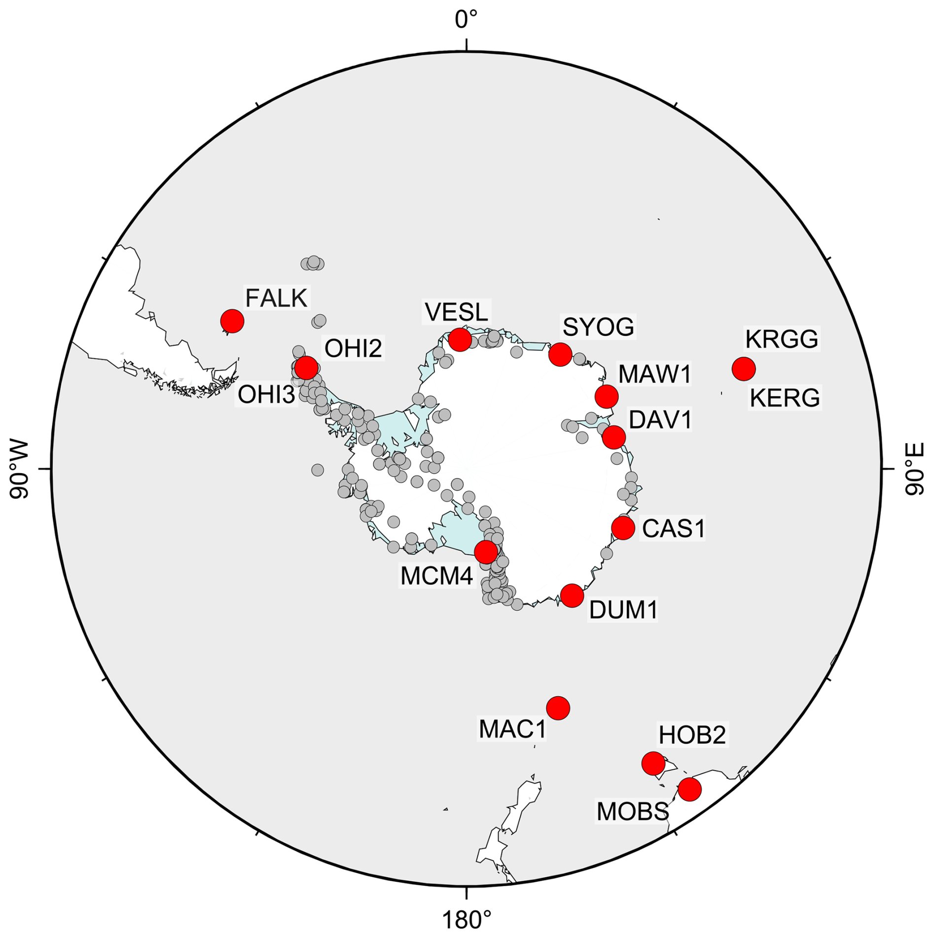
Figure 2 A selection of regionally distributed IGS reference sites to estimate the Helmert parameters of individual AC solutions with respect to the IGb14 reference frame.

Therefore, we applied the linear trends in the HPs on a defined grid covering our region of interest, resulting in point-wise velocities. We then transform the point-wise geocentric velocities to local, topocentric velocities (north, east, and vertical), resulting in the maps depicted in Fig. 3b, which allow for a comparison of the velocity patterns. The OSU and NEWC processing results exhibit a similar pattern, dominated by the rate of translation in Z, resulting in a maximum magnitude of 0.15 mm yr⁻¹ (NEWC) and 0.33 mm yr⁻¹ (OSU) of local subsidence. The TUD pattern shows local vertical rates ranging from 0.27 mm yr⁻¹ to −0.10 mm yr⁻¹, while the lateral velocities are well below 0.20 mm yr⁻¹. The parameters ${\dot{d}}_x$ and ${\dot{d}}_y$ as well as $\dot{\mathit{\alpha }}$ and $\dot{\mathit{\beta }}$ estimated by UTAS are somewhat larger, but they cancel out for our region of interest, resulting in a small lateral deformation pattern with values well below 0.10 mm yr⁻¹ and uplift rates with a maximum of 0.13 mm yr⁻¹.

The differences in the observed patterns can be explained, at least in part, by the application of different reference frame realisation strategies. A maximum consistency with the ITRF is achieved when a globally distributed set of IGS reference sites is used, as is the case for the processing of OSU and NEWC and, inherently, for the PPP solution of UTAS. Nevertheless, differences in the observed pattern are apparent and are of the same order of magnitude as differences with respect to the TUD solution, which relies on a reference frame realisation based on regionally distributed IGS sites. Considering the order of magnitude of the differences in the vertical rate pattern, a straightforward combination of the individual coordinate time series is prohibited to avoid introducing biases. Therefore, we decided to transform all four individual AC solutions using the daily six HPs to a common frame in order to minimise the systematic differences between the solutions.

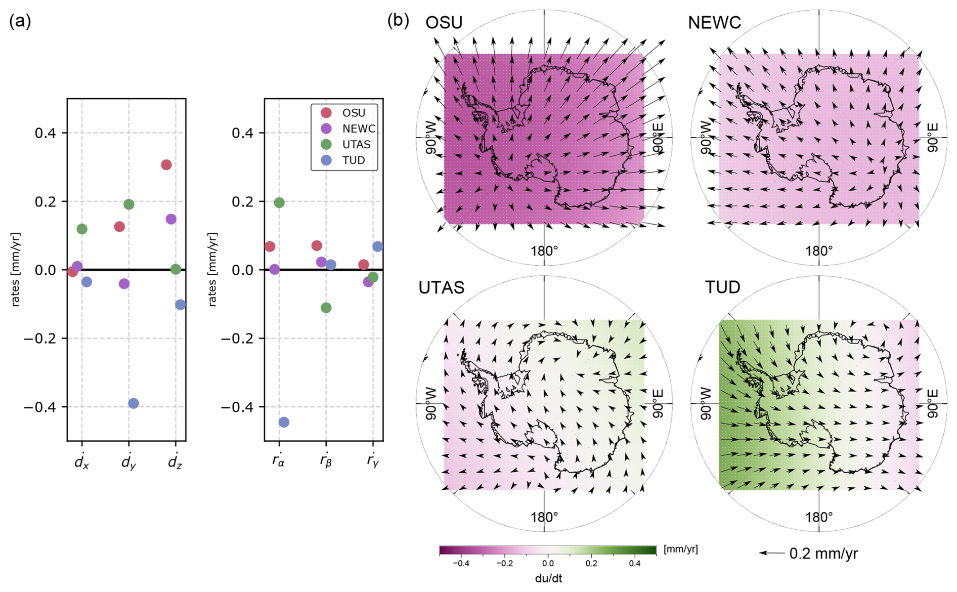
Figure 3 (a) Linear rates of the six Helmert parameters (HPs) for AC solutions with respect to IGb14 based on a selection of regionally distributed IGS sites. The angular velocities ${\dot{\mathit{\alpha }}}_j$, ${\dot{\mathit{\beta }}}_j$, and ${\dot{\mathit{\gamma }}}_j$ are multiplied by the Earth radius to obtain the tangential velocities $\dot{r_{\mathit{\alpha }}}$, $\dot{r_{\mathit{\beta }}}$, and $\dot{r_{\mathit{\gamma }}}$ for better comparability to translation parameters. A positive angle describes a clockwise rotation. The formal uncertainties are negligible, with a range of 1–2 magnitudes smaller than the estimated values. Panel (b) displays the applied linear rates of HPs on a defined grid covering the study area. The coloured grid displays local uplift rates, while arrows show lateral velocities.

3.2.2 Identification of systematically biased solutions

After we minimised the biases between the networks of the individual solutions on the longest timescales, we identified remaining systematic biases between the solutions on a site-by-site basis with a semi-automated procedure. For each site, we formed the median time series over the individual AC solutions for each local topocentric coordinate component (north, east, and up) and computed the differences between each individual solution and the median time series. Sections of continuous time series or campaigns of episodic time series of individual solutions that showed differences larger than 10 mm, 10 mm, or 20 mm in the north, east, or up component, respectively, were flagged. If the flagged solutions could be related to processing choices and could, therefore, be considered to be systematically biased, the biased solutions were excluded from the subsequent combination step. Examples of systematic biases are displayed in Fig. 4. The systematic bias for the UTAS solution (Fig. 4a) following an upgrade to the Septentrio PolaNt-x MF antenna (IGS code: SEPPOLANT_X_MF) and Alertgeo Resolute receivers is evident for every upgraded POLENET station and, therefore, requires the exclusion of the UTAS solution after the upgrade. The TUD analysis included a correction for an antenna misalignment from true north, which is not considered by the other ACs. If the lateral antenna phase centre offsets provided with the igs14.atx file are significant and the antenna misalignment from true north is sufficiently large, the TUD solution shows biases in the lateral coordinate component relative to the other solutions (Fig. 4b). Sections of the TUD solutions showing the described biases were, therefore, excluded from the data combination.

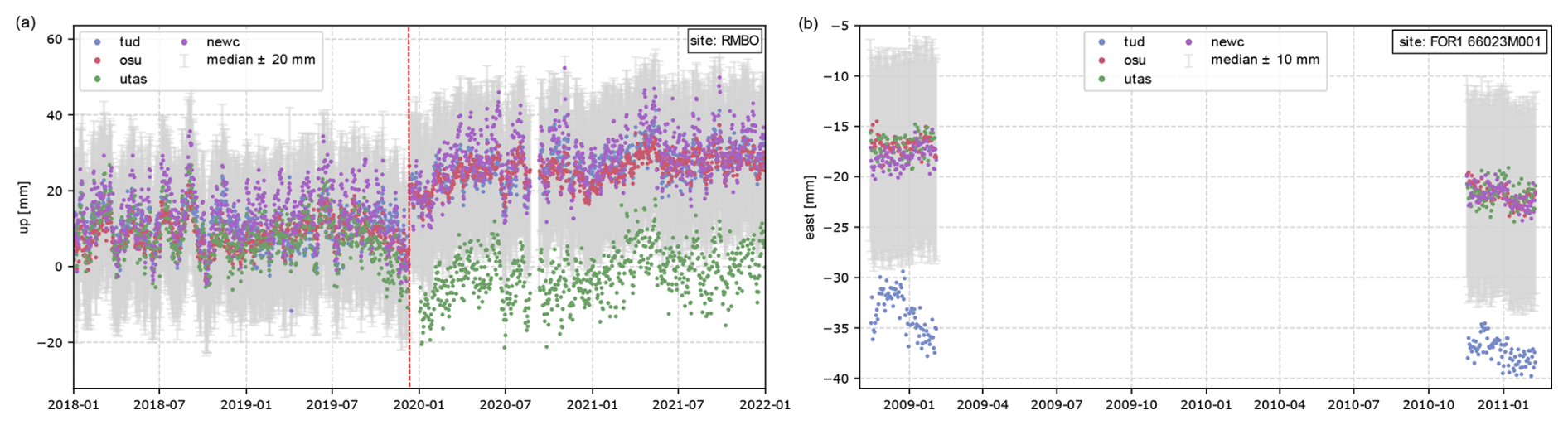
Figure 4 Sections of coordinate time series from the individual AC solutions and the median time series with 20 mm (up) and 10 mm (east) thresholds for the (a) RMBO (up component) and (b) FOR1 (east component) sites. Panel (a) shows a systematic bias in the UTAS solution following an equipment upgrade to the Septentrio PolaNt-x MF antenna and Alertgeo Resolute receiver (11 December 2019). Panel (b) displays the biased east component of the TUD solution, resulting from the correction of the antenna orientation from true north (about 140°), which is only applied in the TUD processing.

3.2.3 Combining the individual coordinate time series

Finally, we combined the individual AC solutions to create the final data set. We implemented a site-wise combination approach by computing the weighted average over the ACs for each geocentric coordinate component:

$$\begin{array}{}\text{(2)}& x(t{)}_{\mathrm{combined}}={\displaystyle \frac{{\sum }_{j=\mathrm{1}}^N{\mathit{\sigma }}_{j,\mathrm{s}}^{\mathrm{2}}\left(t\right)\cdot x_j\left(t\right)}{N\cdot {\sum }_{j=\mathrm{1}}^N{\mathit{\sigma }}_{j,\mathrm{s}}^{\mathrm{2}}\left(t\right)}},\end{array}$$

where ${\mathit{\sigma }}_{j,\mathrm{s}}^{\mathrm{2}}$ is the scaled variance and x_j(t) is the daily geocentric coordinate solution of the AC j. The uncertainties provided with the individual solutions do not provide a realistic measure of uncertainty for the daily coordinate solution. To obtain realistic uncertainty information on the estimated coordinates, error covariance information for the input products (orbits, clock corrections, and tropospheric corrections) would be required to correctly propagate error information to the estimated parameters (e.g. station coordinates). Therefore, the error information provided by each AC has limited meaning in an absolute sense and is not comparable between the AC solutions, although it does contain details about the relative (internal) uncertainty of the individual AC solution. This imposes the necessity to scale the variances for each AC solution. The unscaled variances ${\mathit{\sigma }}_j^{\mathrm{2}}\left(t\right)$ were scaled in such a way that the temporal mean over the scaled variances ${\mathit{\sigma }}_{j,\mathrm{s}}^{\mathrm{2}}\left(t\right)$ of AC j equals the repeatability (variance) of the residual coordinate time series ${\mathit{\sigma }}_{j,\mathrm{res}}^{\mathrm{2}}=\mathrm{var}\left[x_{j,\mathrm{res}}\right(t\left)\right]$:

$$\begin{array}{}\text{(3)}& {\mathit{\sigma }}_{j,\mathrm{s}}^{\mathrm{2}}\left(t\right)={\mathit{\sigma }}_j^{\mathrm{2}}\left(t\right){\displaystyle \frac{{\mathit{\sigma }}_{j,\mathrm{res}}^{\mathrm{2}}}{\stackrel{\mathrm{‾}}{{\mathit{\sigma }}_j^{\mathrm{2}}}}}.\end{array}$$

The advantage of this approach is twofold. First, the scaled variances are related to the repeatability of the residual coordinate time series and therefore have a physical, absolute meaning. Second, the coordinate time series of an AC showing less noise results in a smaller scaled variance and, consequently, higher weighting in the coordinate combination. A limitation of this approach results from the differing temporal coverage and sampling of the individual solutions of the non-stationary coordinate time series.

The required residual coordinate time series were formed by fitting and removing a deterministic trajectory model from the coordinate time series. The trajectory model contains a linear trend, annual and semi-annual signal terms, and (where needed) post-seismic relaxation and a Heaviside step function and, thus, resembles a shortened version of the trajectory model described by Bevis and Brown (2014):

$$\begin{array}{}\text{(4)}& \begin{array}{rl}x\left(t\right)=& \sum _{i=\mathrm{0}}^{n_{\mathrm{P}}}{p}_i(t-t_R{)}^i+\sum _{j=\mathrm{1}}^{n_J}{b}_{j}H(t-t_j)\\ & +\sum _{i=\mathrm{1}}^{n_F}{s}_i\sin \left({\mathit{\omega }}_{i}t\right)+c_i\cos \left({\mathit{\omega }}_{i}t\right)\\ & +\sum _{i=\mathrm{1}}^{n_T}{e}_i(\mathrm{1}-\exp (\mathrm{1}-(t-t_i)/T_i\left)\right)\\ & +\sum _{j=\mathrm{1}}^{n_L}{a}_j\log (\mathrm{1}+(t-t_j)/T_j).\end{array}\end{array}$$

We limit the polynomial degree to n_P=1 and the seasonal harmonics to annual and semi-annual signals. Post-seismic deformation terms were fitted for the BORC and DAL5 sites. The automated identification of steps posed a difficult task (Gazeaux et al., 2013). The limited number of sites within our study allowed for the manual (hand-picked) assessment of steps in the time series. We indicated the time stamps of equipment changes, changes in the antenna eccentricity, the occurrence of nearby earthquakes, and the efforts of sealing antenna ground plates (see Sect. 2.2). If a jump was apparent in one coordinate component, steps were set up for all coordinate components. A full list of events potentially influencing coordinate trajectories is provided with the final data product.

We omitted the seasonal and post-seismic deformation terms for eGPS sites. Additionally, we introduced a jump between each measurement campaign, removing inter-campaign biases. If the inter-campaign biases were not considered in the trajectory model, the residual time series would contain intra-campaign noise and inter-campaign biases. The number of solved measurement campaigns can vary between the AC solutions for eGPS sites. The AC solution that contained more campaigns would, therefore, contain a higher number of inter-campaign biases (if the number of campaigns is larger than two), resulting in an increased residual root-mean-square (RMS) value. An AC solution would be down-weighted in the combination (see Eq. 2) for solving more campaigns.

In a final step, we reduce the combined coordinate time series by the effect of the mean daily NTAL deformation. The computation of the NTAL time series follows the procedure outlined in Sect. 3.1 for the NEWC processing.

3.3 Inference of time series of the zenith total delay (ZTD)

The site-wise tropospheric delay, in the form of the zenith total delay (ZTD), was estimated together with the daily station coordinates by each AC, as described in Sect. 3.1. We provide the site-wise time series of ZTD estimates as an auxiliary data set (Buchta et al., 2024e). The TUD, OSU, and NEWC ACs parameterise the ZTD as piecewise linear functions, leading to duplicate estimates at the day boundaries. To form a continuous time series, the estimates for each AC were averaged at the day boundaries. The high-rate UTAS solution was down-sampled by forming hourly averages. Here, we decided against the combination of ZTD results and, instead, provide the individual AC solutions.

4 Results

4.1 Combined coordinate time series

As the major product, we provide the combined coordinate time series for 286 bedrock sites in Antarctica (Buchta et al., 2024b). The individual ACs provided solutions for 286 (TUD), 286 (UTAS), 258 (OSU), and 270 (NEWC) sites. The differences in the number of solutions are due to different approaches and thresholds concerning the quality or completeness of the observational data. The combination leads to a small increase in the total number of daily solutions. The comparison of the number of daily solutions per site between the combination and the individual solution with the most solutions results in a mean increase of 0.3 %. The resulting mean time base of the combined product is 10.5 years. Figure 5 shows an example coordinate time series comprising both the individual and combined solutions. To assess the repeatability and noise characteristics of the individual and the combined solutions, we analysed the coordinate time series of 29 stable cGPS sites. These sites were selected to cover a time span of at least 6 years, to have no reported snow intrusions, to not be subject to other external disturbances, and to be well distributed over the Antarctic continent (see Fig. 6).

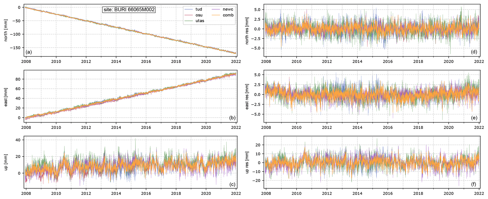
Figure 5 Coordinate time series (a–c) and the residual time series (d–f) for the Butcher Ridge (BURI) site from the individual AC solutions and the combined final time series. The RMS of the residual time series of the combined solution yields 1.0, 1.1, and 4.6 mm for the north, east, and up components, respectively. The individual solutions with lowest RMS reach values of 0.9 mm (NEWC), 0.9 mm (OSU), and 3.6 mm (OSU) for the north, east, and up components, respectively.

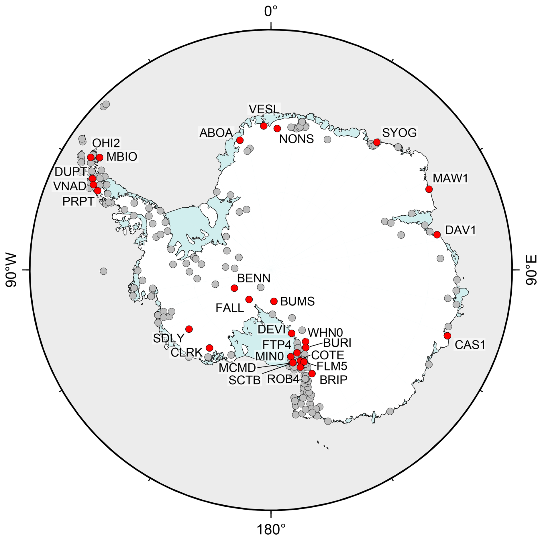
Figure 6 Selection of 29 stable cGPS sites (red) to assess the noise characteristics of coordinate time series of the ACs and the combined solution.

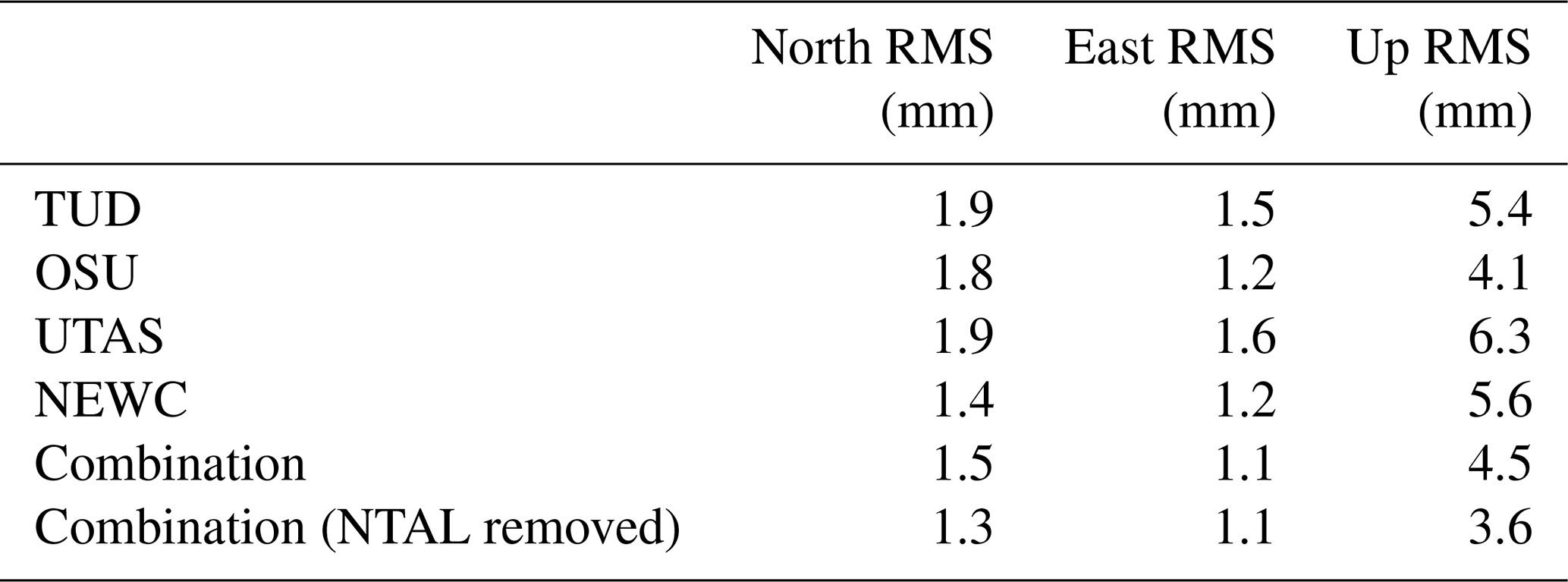
First, residual time series were formed by fitting and subtracting a deterministic model (Eq. 4) from the time series (see Fig. 5 for an example time series). Post-seismic deformation terms were neglected for the selected sites. Steps were consistently introduced for all ACs and the combined time series. The repeatability of the coordinate time series is then described by the derived RMS over the residual time series. Table 1 displays the median RMS for each AC and the combined solutions. The NEWC solution shows the lowest RMS for the lateral components, with a median RMS of 1.4 and 1.2 mm for the north and east components, respectively. The solution of OSU reaches the smallest median RMS for the vertical coordinate component with 4.1 mm. The repeatability for the TUD and UTAS solutions show higher values for the north and up components. The RMS values of the combined time series resemble the lowest RMS of the best-performing individual solutions for the lateral components with −0.1 and −0.1 mm for the north and east components, respectively, compared to the best-performing individual solution. The RMS for the vertical component is found to be 0.4 mm larger than that of the OSU solution.

Table 1 The median of the repeatability (RMS) derived from residual coordinate time series for the north, east, and up coordinate components for a selection of 29 stable continuous sites.

To further characterise the spectral properties of the residual time series, we calculated the Lomb–Scargle periodogram (LSP), a representation of the power-spectral density for non-uniformly sampled data (VanderPlas, 2018). We used un-normalised LSPs where the power-spectral density takes values similar to those of a fast Fourier transform (FFT) analysis, differing by a factor of 2 in the case of a complete time series. LSPs were computed for all sites and each coordinate component for each AC and for the combined solutions. Subsequently, the median LSP was formed over all 29 sites, allowing for the direct comparison between the solutions (Fig. 7).

Firstly, the periodograms confirm the generally lower noise levels of the lateral coordinate components of the NEWC and OSU solutions compared to the TUD and UTAS solutions, especially at high frequencies. All solutions follow the well-known power-law-like behaviour of GPS coordinate time series, close to flicker noise (spectral index equals −1) and white noise for very high frequencies (Liu et al., 2018; King et al., 2022). Differences between the solutions become apparent for distinct frequencies. Dominant peaks are visible for the otherwise very low noise periodograms of the NEWC (north, east, and up) and OSU (east) solutions at the fortnightly periods of 13.63 and 14.16 d, possibly resulting from “direct” and “indirect/aliased” errors in tidal models (Ray et al., 2013). Smaller peaks are visible at 9.4 d for UTAS (up) and at 9.14 d for NEWC (up), also resulting from direct and indirect errors in tidal models, respectively. At lower frequencies, distinct peaks at harmonics of the GPS draconitic year (351 d) are apparent (Ray et al., 2008). The combined time series reveals reduced amplitudes for the spurious signals at high frequencies, whereas the draconitic harmonics remain at high amplitudes. Combining the individual solutions, as described in Sect. 3.2.3, has several advantages over the individual solutions: the repeatability is similar to the best-performing single AC solution, the amplitudes of high-frequency interfering signals have been reduced, and the overall spatiotemporal coverage has been increased.

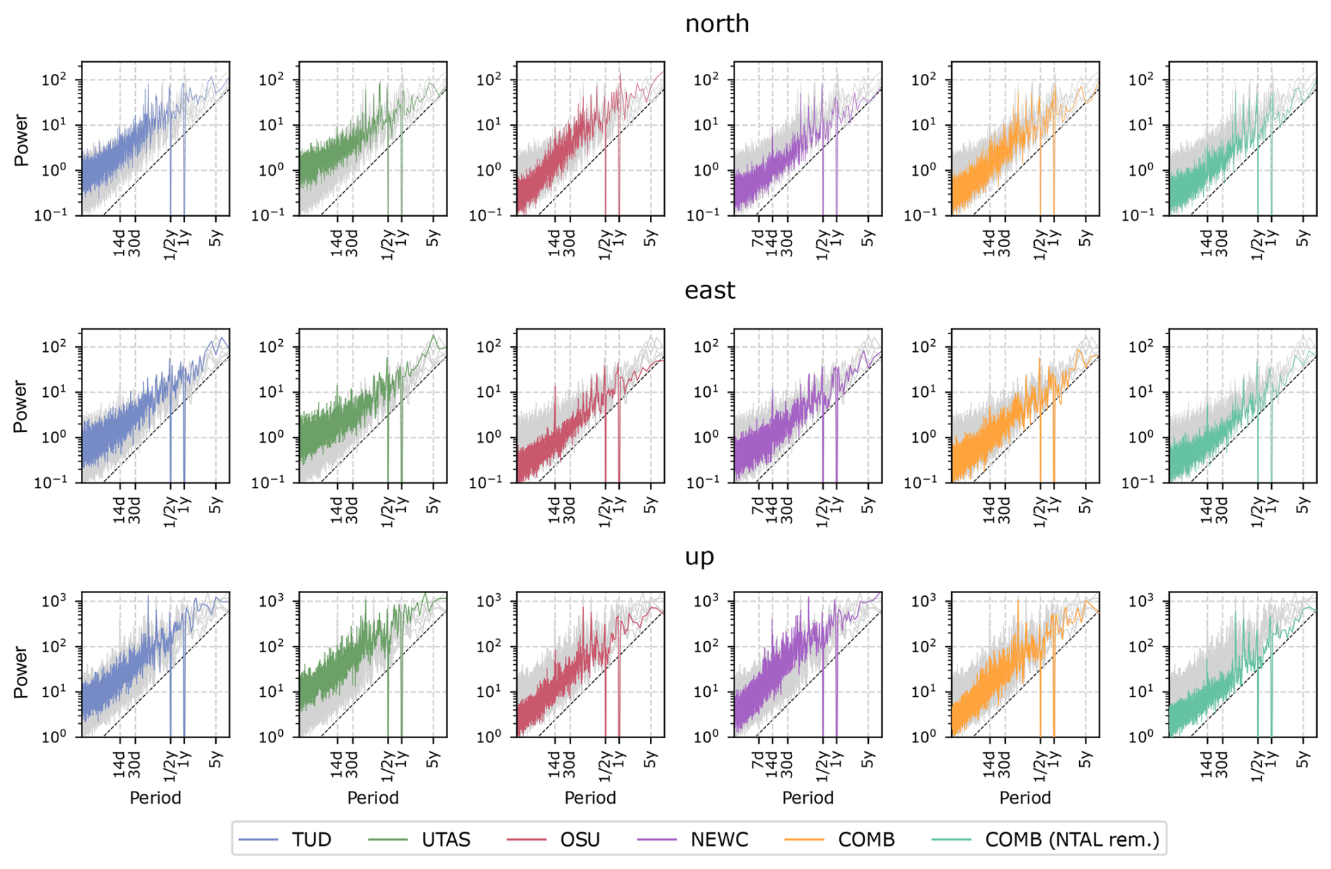
Figure 7 Median Lomb–Scargle periodograms (LSPs) of residual time series (east, north, and up) for the selection of 29 cGPS sites for the four ACs and the combined solution with and without NTAL removed. Each plot displays the LSP of a specific solution in colour and the LSPs of the other solutions in grey. The dashed line displays flicker noise with an arbitrary amplitude.

The effect of NTAL-induced deformations was removed from the combined coordinate time series to infer the final data set. A number of studies have discussed the influence of NTAL effects on GPS time series, leading to a reduction in the amplitude of annual signals and the residual RMS depending on the site location (Männel et al., 2019; Mémin et al., 2020). For the selection of stable sites, we find a mean reduction in the residual RMS of 0.2, 0.0, and 0.9 mm (see Table 1) and a mean reduction in the annual amplitude of 0.1, 0.0, and 0.6 mm for the north, east, and up components, respectively. The maximum reduction in the vertical annual amplitude of 2.5 mm was found for the FALL site. An increase in the annual amplitude was identified for sites in Dronning Maud Land, with a maximum of 1.6 mm for the ABOA site.

We realised the terrestrial reference frame IGb14 using a regional selection of reference sites for the individual AC solutions (see Sect. 3.2.3). As shown by Legrand et al. (2010), using a sparse set of regionally distributed reference sites can introduce a (secular) bias in the coordinate solutions. This adds to the uncertainty in the reference frame itself, which shows a secular bias of 0.2 mm yr⁻¹ on the polar axis when comparing ITRF2014 to ITRF2020 (Altamimi et al., 2023). Uncertainties in the reference frame realisation, especially on the Z axis, map onto the uncertainty in the local vertical coordinate component of sites in the polar regions and must be taken into account when using them for geodynamic studies (e.g. GIA).

4.2 Comparison to the data set of the Nevada Geodetic Laboratory (NGL)

In order to evaluate our results using an independent solution, we compared and validated the results of our GIANT-REGAIN (GR) combined solution with the data products of the Nevada Geodetic Laboratory (NGL), University of Reno (Blewitt et al., 2018). Their publicly available “living data set” consists of coordinate time series of more than 17 000 globally distributed GPS stations with more than 10 000 stations updated every week. The NGL processing employs the PPP processing strategy of the GipsyX software, which provides a computationally efficient method to process an immense number of data. The processing uses GPS observations only as well as JPL orbit and clock products (Earth orientation parameters, satellite clocks, and ephemerides). The coordinate solutions are realised in the IGS14 reference frame. We refer to web resources (http://geodesy.unr.edu/gps/ngl.acn.txt, last access: 2 August 2024) for further details on the NGL processing set-up. In their solutions, the critical metadata (including antenna types and heights) are extracted from the header section of RINEX observation files.

To compare the data sets we selected 157 sites (55 % of the GR data set) available in both data sets and downloaded the final, cleaned NGL time series of geocentric coordinates (Fig. 8). For this comparison, neither data set was corrected for NTAL deformation.

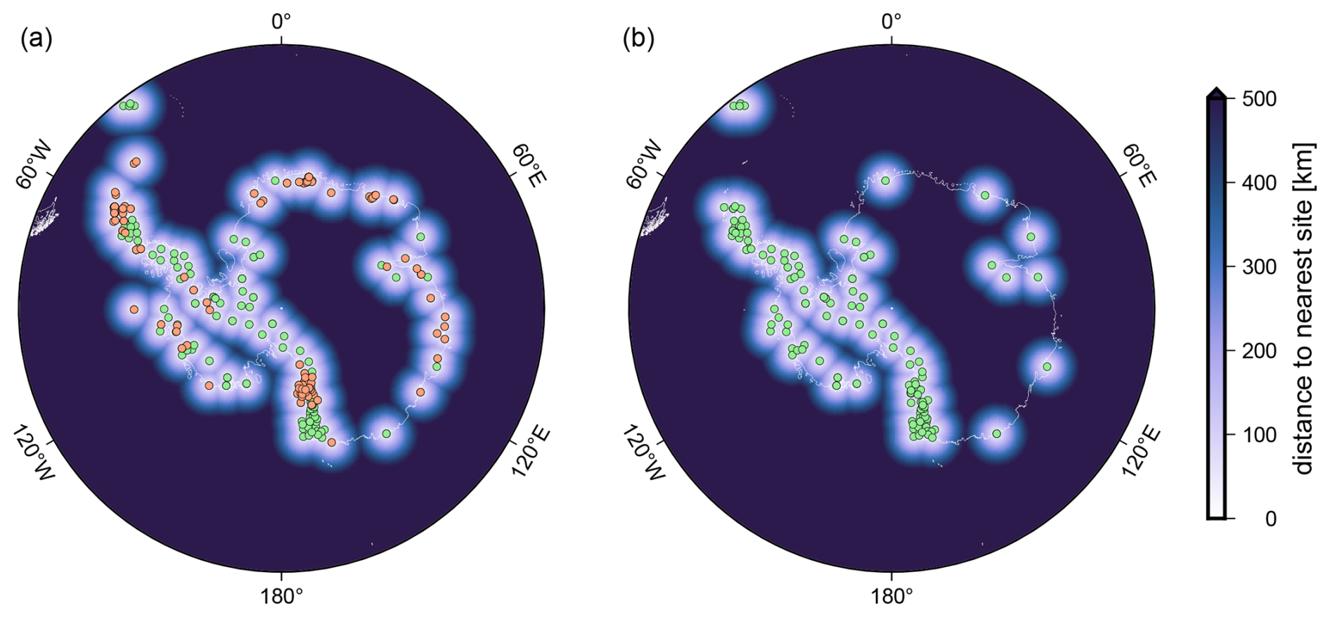
Figure 8 GPS station coverage of (a) the GIANT-REGAIN (GR) data set and (b) the Nevada Geodetic Laboratory (NGL) data set. Green markers indicate GPS sites included in both data sets, while orange sites are only included in the GR data set. The GR data set has an enhanced spatial coverage for East Antarctica from 30° W to 100° E and an increased station density for southern Victoria Land and the northern Antarctic Peninsula.

To check the consistency of the data sets, we compared the linear rates of coordinate change derived from both data sets. For this purpose, the NGL data set is limited to the GIANT-REGAIN period from 1995 day of year (DOY) 001 to 2021 DOY 365. Further, we limited the analysed stations to those that have an observation span of at least 3 years in both data sets, resulting in a selection of 143 sites. We used the local topocentric coordinate representation (north, east, and up) for the analysis. The Hector software package v1.9 (Bos et al., 2013) was used to fit a deterministic model (Eq. 4) to the time series, while assuming a white and flicker noise stochastic model. The deterministic model is limited to a linear trend and potential offsets for eGPS sites. We extracted information on discontinuities for the NGL data set from the provided master step file database (http://geodesy.unr.edu/NGLStationPages/steps.txt, last access: 2 August 2024). Steps in the GR data set are consistent with those used in Sect. 3.2.3.

Sites with large trend differences exceeding 10 mm yr⁻¹ in either the north, east, or up components were considered outliers and excluded from the subsequent analysis. Five sites exceeded this threshold: MBL3, SLTR, VL06, VL20, and VLHG. The large differences can be explained by different assumptions regarding antenna heights and the different identification of jumps in the GR and NGL data sets. The distribution of trend differences (GR – NGL) for the remaining stations reveals a high level of consistency (Fig. 9). The mean differences and standard deviations can be considered small, with values of 0.1±0.6, 0.0±0.8, and 0.2±1.1 mm yr⁻¹ for the north, east, and up components, respectively. The estimated rates are sensitive to the assumed steps in the deterministic models. We repeated the estimation of the trends for the NGL data set but introduced step information consistent with the GR data set. The increased consistency of the deterministic models leads to a further reduction in the trend differences for the lateral components to 0.0±0.4 and 0.0±0.5 mm yr⁻¹ for the north and east components, respectively. The differences in the estimated rates reflect differences a user would obtain using either data set for the defined time span. They do not solely describe differences that result from the different processing strategies. Individual site time series may have different temporal coverage for either data set and, therefore, be affected differently by non-linear loading variations (Koulali et al., 2022; King et al., 2022).

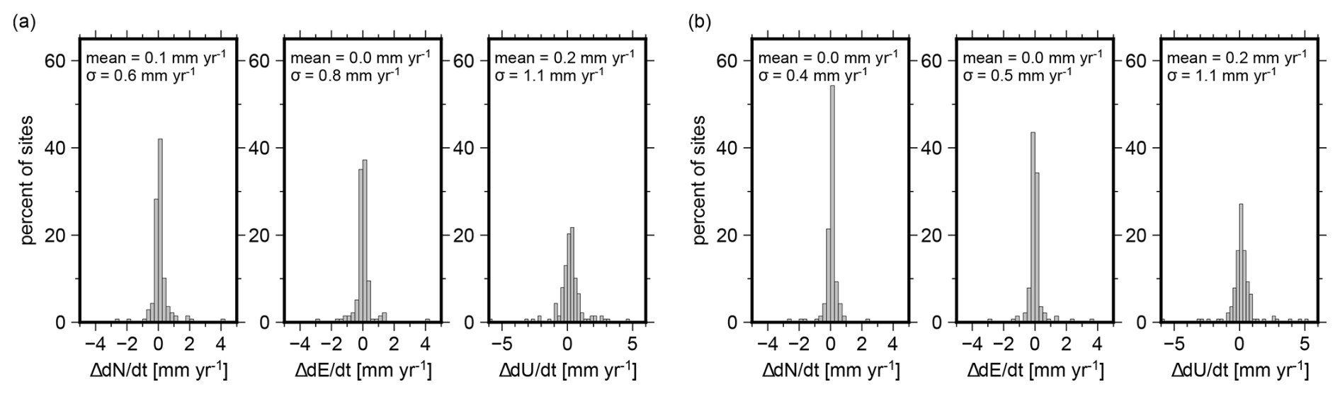
Figure 9 Distribution of differences in estimated linear rates between GR and NGL. In panel (a), the steps in the NGL data set are considered in accordance with the NGL master step file. Conversely, in panel (b), the step information for NGL is consistent with the GR data set.

The NGL data set originates from a highly automated processing and retrieves the necessary metadata from the header section of the observational RINEX file (Blewitt et al., 2018), which can be prone to errors. The NGL data set provides antenna heights along with the coordinate time series, enabling comparison with the revised metadata information of the GR data set. The comparison reveals different antenna heights for 57 sites and antenna height differences greater than 4 mm (approximate noise level of the up component; see Table 1) for 43 sites, equaling 36 % and 27 % of sites, respectively. Differences in the antenna heights do not necessarily result in differences in estimated trajectory models, e.g. if the antenna height difference is constant for the whole observation time or between estimated steps. We quantify the impact of the improved antenna height information by modifying the NGL time series of the up component u_NGL(t) for the 57 sites as follows:

$$\begin{array}{}\text{(5)}& u_{\mathrm{NGL}}^{\mathrm{mod}}\left(t\right)=u(t{)}_{\mathrm{NGL}}+H_{\mathrm{NGL}}(t)-H_{\mathrm{GR}}(t),\end{array}$$

where H_NGL(t) is the antenna height provided by NGL at time t and H_GR(t) is the antenna height provided by the GR data set at time t. We detrended u_NGL(t) and $u_{\mathrm{NGL}}^{\mathrm{mod}}\left(t\right)$ and computed the residual RMS for all 57 sites. The mean RMS shows a reduction from 21.3 mm to 8.5 mm, while the median RMS shows a reduction from 9.1 to 7.9 mm. The RMS reduction results from the correction of outliers and the reduction in the steps associated with antenna changes. Example coordinate time series displaying the effect of corrected antenna heights are given in the Supplement.

5 Data availability

The product inferred by this project is available at the PANGAEA repository (https://doi.org/10.1594/PANGAEA.967515, Buchta et al., 2024a) as a data set collection and comprises four individual data sets: the combined coordinate time series (https://doi.org/10.1594/PANGAEA.967516, Buchta et al., 2024b); the time series of the tropospheric zenith total delay (ZTD) from the individual AC processing results (https://doi.org/10.1594/PANGAEA.967529, Buchta et al., 2024e); the station information in the form of IGS log files (https://doi.org/10.1594/PANGAEA.967532, Buchta et al., 2024d); and a list of events (https://doi.org/10.1594/PANGAEA.967533 Buchta et al., 2024c), which can be employed in conjunction with the coordinate time series data to analyse the coordinate trajectory. The data sources of publicly available observational data are listed in Table S1 in the Supplement.

6 Code availability

The GNSS analysis software used is available from the relevant research groups. Parallel.GAMIT is available at https://github.com/demiangomez/Parallel.GAMIT (Gómez, 2024).

7 Conclusions

We collected and evaluated observational data and station metadata for 286 GPS sites in Antarctica from 1995 to 2021. The processing of the data was carried out by four analysis centres. This allowed us to maximise the temporal and spatial coverage of our data set and to identify possible biases in individual solutions. In this way, we were able to generate a consistent combined data set of coordinate time series. Compared to the data set provided by the Nevada Geodetic Laboratory (NGL), which contains the largest number of GNSS sites in Antarctica to date, we were able to increase the spatial coverage, especially in East Antarctica. In some regions, such as Victoria Land and the Antarctic Peninsula, the comparably high density of stations could be increased even more. Our revised station metadata decrease the number of artefacts (e.g. outliers and jumps) in the coordinate time series and provide the basis for a reliable analysis of episodic (eGPS) sites.

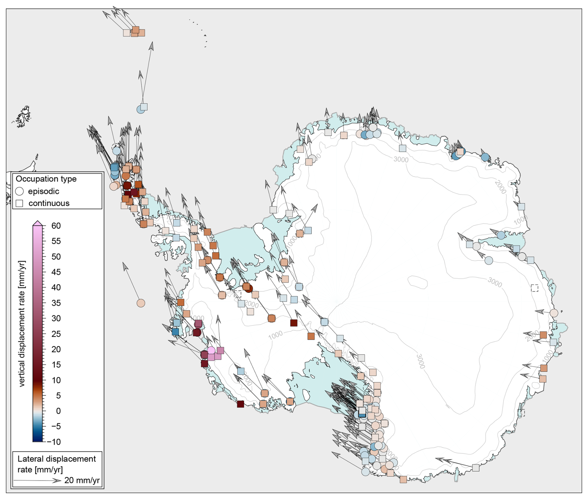
Figure 10 Horizontal and vertical displacement rates resulting from a preliminary analysis of the combined coordinate times series (NTAL removed) using the trajectory model as discussed above. Linear rates were estimated with the Hector software (Bos et al., 2013) using a flicker+white noise model. Only sites with a time base larger 2.5 years and more than 10 data points were analysed. Note that these rates still contain all geodynamic effects, such as (1) the response of the solid Earth to past and present-day ice-mass loading and unloading or (2) plate kinematics. Sites are displayed with dashed outlines if no rate was estimated.

The main product – a consistent GPS coordinate time series – is supplemented by the data sets of time series of the zenith total delay as well as the station metadata in the form of IGS log files and a station event list. The latter is intended to serve as a possible starting point for analysing and interpreting the coordinate trajectory, as it contains information on equipment changes, nearby earthquakes, and measures taken to mitigate snow contamination of the GPS antennas.

The inferred consistent coordinate time series will advance the investigation of various geodynamic effects on different timescales. Derived linear rates may be employed to examine plate motion or to validate and constrain models of GIA. The enhanced spatial and temporal coverage of this data set will allow one to assess GIA models more rigorously than previously possible. This pertains to the spatial coverage, notably in East Antarctica, as well as the augmented station density in regions of increased lateral gradients in the vertical uplift rates, exemplified by the northern Antarctic Peninsula (Koulali et al., 2022) and the Amundsen Sea region (Barletta et al., 2018). However, the isolation of the GIA signal, in particular in the vertical component, requires the removal of the instantaneous (elastic) deformation caused by the present-day mass change, i.e. superimposed loading due to the SMB and changes in ice dynamics (Hattori et al., 2021; Koulali et al., 2022; King et al., 2022), which is not within the scope of the study. Therefore, we do not provide a product of secular rates from the coordinate time series. However, to demonstrate the potential of the data set, we derive linear rates for all sites with a time base larger than 2.5 years and at least 10 data points (Fig. 10), using the trajectory models described in Sect. 3.2.3.

Furthermore, this data set, especially the derived station metadata, will serve as a baseline for anticipated future reprocessing efforts, which could then consider an up-to-date ITRF realisation and associated conventions, extend the coordinate time series of existing stations, and include new GPS stations in the data set. The compilation of all available GPS data provides an unprecedented insight into solid-Earth deformation in Antarctica. The comprehensive overview (e.g. Fig. 8) highlights gaps in GPS coverage and will be used to plan future station deployments to further improve coverage and maintenance of the geodetic infrastructure.