Airborne gravimetry with quantum technology: observations from Iceland and Greenland

We report on the availability of data from an airborne gravity campaign in Iceland and Greenland conducted during June and July 2023. The dataset includes observations from a platform-stabilised gravimeter based on cold-atom quantum technology and a strapdown gravimeter based on classical technology. The data are available at three different levels of processing, making them relevant to users interested in working with “quantum” and “hybrid” data as well as users interested in geophysical studies. The paper describes the data processing applied to derive the various levels of data and presents an evaluation of the accuracy of the data. This evaluation indicates an accuracy of 1–2 mGal for both sensors, depending on the roughness of the gravity field. Although the two technologies lead to similar performance, further analysis indicates that the error characteristics are different and that the final estimates would benefit from a combination (data available at https://doi.org/10.57780/esa-58c58c5; see Jensen et al., 2024).

1 Introduction

This paper reports on the data available from an airborne gravity campaign carried out in the summer of 2023. Airborne gravimetry is a powerful tool for measuring gravity at regional scales where ground measurements are difficult, such as mountains or coastal areas. Recently, a new technology of airborne gravimeters based on cold-atom quantum technology emerged. Unlike classical technologies that can only measure the relative variation of gravity from an aircraft, a quantum gravimeter provides a direct absolute measurement of gravity, eliminating the need for calibration and drift estimation. Here we present airborne gravity measurements over Iceland and Greenland using quantum and classical gravimeters.

The campaign was a result of merging two projects targeting locations in Iceland and Greenland but carried out using the same instrumentation. The main instrument is the GIRAFE quantum gravimeter developed by the French Aerospace Lab (ONERA), accompanied by the iMAR iNAT-RQH strapdown gravimeter (Jensen, 2024) owned by the National Space Institute at the Technical University of Denmark (DTU Space). Two similar campaigns were previously carried out in 2017 (Iceland) and 2019 (France), both of which remain the only ones of their kind reported in the literature (Bidel et al., 2020, 2023). The current campaign contains a repetition of the previous campaign in Iceland, making it possible to directly evaluate the improvements implemented since the first airborne test in 2017.

With the GIRAFE sensor being the only one of its kind, the technology remains at the development stage. For this reason, the data are made available at three different levels of processing, making them relevant for several users. The level-0 data are the raw observations collected during the campaign, relevant for users aiming to perform their own data processing. The level-1 data contain several intermediate variables, relevant for users aiming to develop their own processing software or interested in tuning some processing parameters for specific purposes. The level-2 data contain the final gravity estimates from the campaign, relevant for users aiming at geophysical studies or gravity field modelling. The data are made available by the European Space Agency (ESA), and these data levels are similar to other data products available through their servers (Jensen et al., 2024).

Following the introduction, Sect. 2 gives a brief description of the airborne campaign and the instrumentation. Section 3 introduces some fundamental theory and a data processing strategy applied to transition from level-0 to level-2 data. Additionally, some means of evaluating the accuracy of the level-2 gravity estimates are described. Finally, the obtained results are presented in Sect. 4, which also aims to give some insights into the characteristics of the data. This section is followed by a conclusion and a statement of data availability.

2 Survey overview and instrumentation

As a result of merging two projects, the measurement campaign consists of two separate geographical locations, i.e. Iceland and Greenland. The base airport of operation was located in Akureyri (AEY) in Iceland, from where all the instruments were installed on the chartered DHC-6 300 Twin-Otter aircraft. Following installation and testing, survey flights in Iceland were carried out. These flights are part of the AirQuantumGrav project funded by ESA. Afterwards, the aircraft was transferred to Nuuk in Greenland, from where a survey of the surrounding fjord system was carried out. This second part of the campaign belongs to the Green Quantum project funded by the Danish Ministry of Defense Acquisition and Logistics Organization (DALO). Below is a short overview of the two projects along with the instrumentation installed on board the aircraft.

2.1 The AirQuantumGrav project

The main objective of the AirQuantumGrav project was to pursue the quantum technological benefits of stability, absolute measurements, and no calibration needs for airborne gravimetry. The project builds upon an earlier one such that flight lines from a previous campaign in 2017 are repeated (Bidel et al., 2020; Bresson et al., 2023). The current project identified the following targets for the 2024 campaign:

• a repetition of the 2017 airborne campaign over the Vatnajökull ice cap;

• an overflight of the Askja volcano;

• an overflight of the Fagradallsfjall volcano; and

• a repetition of the 2017 flight line from Snæfellsjökull to Akureyri.

All of the target locations are sources of mass variation due to known geophysical phenomena, i.e. a melting ice cap, rapid uplift, and volcanic activity. The repetition of such targets would enable the investigation of mass variation, assuming that the accuracy is sufficient. An overview of the flights carried out within the project is shown in Fig. 1.

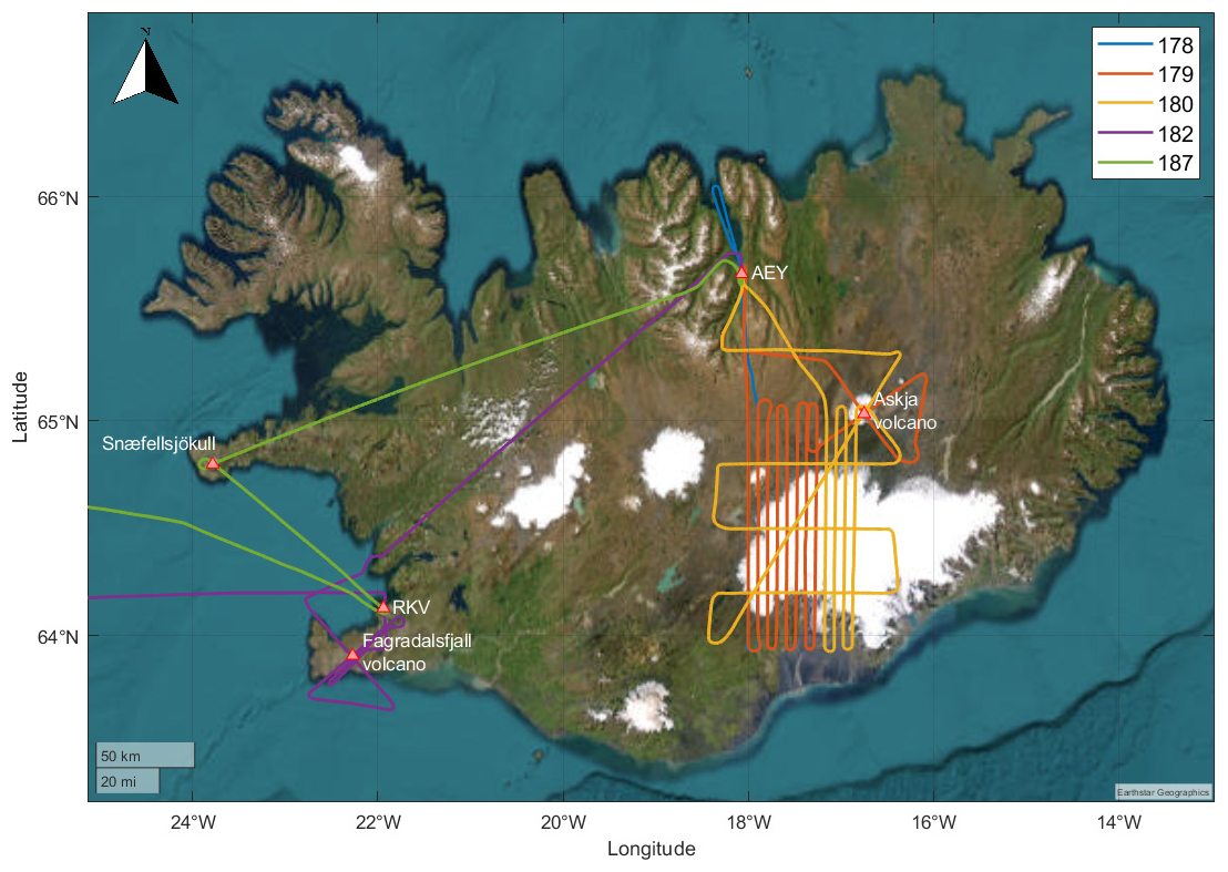
Figure 1 Ground track from flights in Iceland. The legend refers to the day of the year. Also shown are the locations of the Askja, Snæfellsjökull, and Fagradalsfjall volcanoes along with Akureyri airport (AEY) and Reykjavik domestic airport (RKV).

2.2 The Green Quantum project

The Green Quantum campaign was planned as a regular grid survey, with the purpose of mapping the gravity field with a uniform spatial resolution over the area. The data collected in the area will be used as input for the computation of a new Geoid model for the Nuuk region and later for updating the vertical reference frame of Greenland. The ground tracks from the flights are shown in Fig. 2.

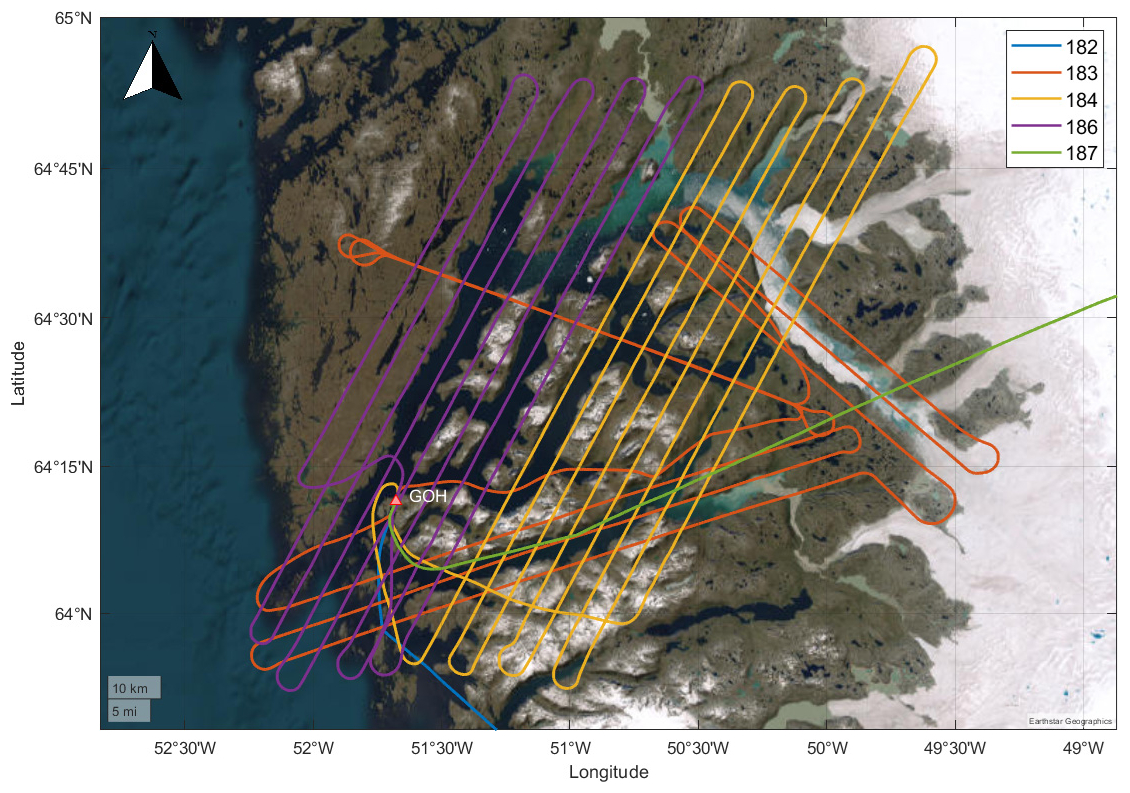
Figure 2 Ground track from flights covering the Nuuk fjord system in Greenland. The legend refers to the day of the year. Also shown is the location of the Nuuk airport (GOH).

The campaign additionally serves to support the ADEQUADE project funded by the EU-EDF programme. For this the east–west flight line was repeated four times, testing the quantum gravimeter with the stabilising platform active and inactive.

2.3 Instrumentation

On board the aircraft were installed two gravimeters along with three different Global Navigation Satellite System (GNSS) receivers. The main instrumentation was the GIRAFE cold-atom quantum gravimeter developed by ONERA.

The GIRAFE gravimeter is based on the measurement of the acceleration of a cloud of cold atoms in free fall using matter wave interferometry. A detailed description of this technology can be found in Tino and Kasevich (2014). The description of GIRAFE is given in Bidel et al. (2018, 2020, 2023). The main advantage of the quantum gravimeter compared to classical technologies is the ability to provide an absolute value of the acceleration, which means that the instrument does not require calibration or drift estimation. Traditionally, an airborne gravity survey requires calibrations before and after each flight, thus depending on external gravity values from either an existing gravity network or additional absolute gravity measurements taken at the airport. The independence of such an infrastructure is a major operational advantage.

To represent the classical technology, an iMAR iNAT-RQH strapdown gravimeter (Jensen, 2024) was installed adjacent to the platform-based quantum gravimeter. Both sensors are illustrated in Fig. 3. The strapdown gravimeter is essentially a navigation-grade inertial measurement unit (IMU) that is rigidly fixed to the chassis of the aircraft. Since no active platform ensures that the sensor remains aligned with the direction of the gravity vector, the orientations of three perpendicular sensors are computed during data processing in order to resolve the gravity acceleration. This will be elaborated on in Sect. 3.1.

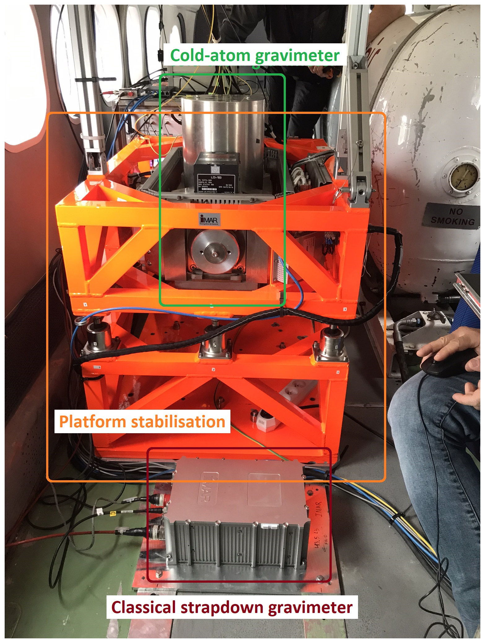
Figure 3 Photograph of the installation of the two gravimeters. The GIRAFE cold-atom gravimeter is mounted on a stabilising platform, while the iMAR strapdown gravimeter is rigidly attached to the aircraft floor.

In addition to the gravimeters, three GNSS receivers were installed and connected to the same GNSS antenna on top of the aircraft. Contrary to stationary gravimetry, the GNSS observing system is essential for moving-base gravimetry, and gravity cannot be derived without it (or other systems for determining motion-induced accelerations). The three receivers installed on the aircraft were

• a Javad Delta GNSS receiver (GPS and GLONASS only),

• a Septentrio Mosaic-Go GNSS receiver (multi-constellation), and

• a NovAtel PwrPak7 GNSS receiver (multi-constellation).

Additionally, a Javad Triumph GNSS receiver was placed in the airport whenever possible. This may serve as a base station for differential processing on most flights. Note however that the receivers differ in which satellite constellations they are able to receive data from and which observation type is logged on the unit.

Finally, in order to power and operate the various instruments, several cabinets with electronics were installed on the aircraft along with the equipment. A sketch of the installation is illustrated in Fig. 4.

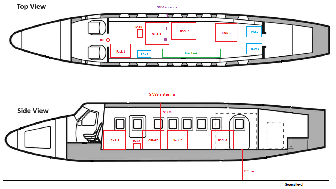
Figure 4 Sketch of the aircraft installation with placement of the iMAR and GIRAFE gravimeters relative to the GNSS antenna.

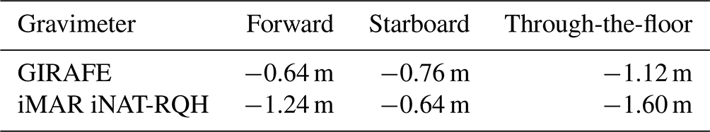
One important parameter for the data processing is the physical separation between the gravity sensors and the GNSS antenna located on top of the aircraft. These distances, generally denoted the lever arm, were estimated during data processing by adding them as constant variables in the state vector during the combination of GNSS and IMU observations. The estimates are listed in Table 1.

Table 1 Estimates of lever arms from the two gravity sensors to the location of the GNSS antenna. Distances are along the forward, starboard, and through-the-floor directions of the aircraft.

3 Methodology

This section begins with a short summary of the theoretical principles of airborne gravimetry. This is followed by a section outlining the processing methodology along with two sections describing methods for internal and external validation of results. Finally, a section describing a simple method for combining estimates from two sensors is included.

3.1 Moving-base gravimetry

As mentioned in Sect. 2.3, the essential instruments for the campaign are the two gravimeters. Such gravimeters measure specific force accelerations, f^s, along the axes of a sensor reference frame (s frame). The specific force represents acceleration originating from both movement and gravitation, such that

$$\begin{array}{}\text{(1)}& {\displaystyle }{\displaystyle }{\mathit{f}}^i={\mathbf{C}}_s^i{\mathit{f}}^s={\ddot{\mathit{r}}}^i-{\mathit{g}}^i,\end{array}$$

where the kinematic acceleration, $\ddot{\mathit{r}}$, is expressed as the double derivative of position r with respect to time. The transformation matrix, ${\mathbf{C}}_s^i$, represents a rotation of the sensor-frame axis (s frame) onto the axes of an inertial reference frame (i frame). The above expression is valid in an inertial reference frame only, which is denoted using the superscript i. An accelerometer measures along a single axis in space such that three perpendicular accelerometers are needed in general to measure the full vector quantity. These three values are thus obtained along the axes of the s frame, which may have any orientation in space.

Data processing is done in the navigation frame (n frame) centred at the instrument location with axes along the local northerly, easterly, and downwards directions. For this we need to first project the observed accelerations onto the axes of the n frame as

$$\begin{array}{}\text{(2)}& {\displaystyle }{\displaystyle }{\mathit{f}}^n={\mathbf{C}}_s^n{\mathit{f}}^s,\end{array}$$

where ${\mathbf{C}}_s^n$ is a rotation operator. In practice, ${\mathbf{C}}_s^n$ need not be computed after processing but can be applied in real time by continuously rotating the instrument such that its axes are always aligned with the northerly, easterly, and downwards directions. The stabilising platform of the GIRAFE instrument represents such a real-time solution, although it only rotates about two axes in order to align the gravity sensor with the local vertical. The iMAR strapdown instrument on the other hand additionally contains three perpendicular gyroscopes, measuring rotations such that the orientation of the instrument (i.e. the ${\mathbf{C}}_s^n$ matrix) can be computed after the mission.

Additionally, we need to modify Eq. (1) in order to comply with the n frame by considering relative movement between the i and n frames. Here two terms arise, one originating from the rotation of Earth with respect to inertial space and one from the rotation of the navigation frame in order to keep it aligned with the local northerly and downwards directions as we move across the surface of Earth (Groves, 2013). Collectively, these terms are known as the Eötvös effect:

$$\begin{array}{}\text{(3)}& {\displaystyle }{\displaystyle }{\mathit{E}}^n=\left(\mathrm{2}{\mathbf{\Omega }}_{ie}^n+{\mathbf{\Omega }}_{en}^n\right){\mathit{v}}^n,\end{array}$$

where ${\mathbf{\Omega }}_{ie}^n$ and ${\mathbf{\Omega }}_{en}^n$ are skew-symmetric matrices of the rotational rates mentioned above, while vⁿ is the velocity resolved about the n-frame axes. As a kind of mental argument we may imagine this to be a correction term due to the choice of reference frame. For example, imagine a sensor stationary on the surface of Earth. In this case we would want the velocity to be zero and the position to be constant. However, the accelerometer measures with respect to inertial space, meaning that it will measure some acceleration due to the rotating Earth. If one would simply integrate the accelerations with respect to time, we would obtain a changing velocity and position in time. In order to cancel this effect, we need to introduce a fictitious correction term into the accelerations before integrating. This is the Eötvös effect.

Finally, we may piece together the above terms to form the following fundamental equation of gravimetry (Jekeli, 2001):

$$\begin{array}{}\text{(4)}& {\displaystyle }{\displaystyle }{\mathit{g}}^n={\ddot{\mathit{r}}}^n-{\mathbf{C}}_s^n{\mathit{f}}^s+\left(\mathrm{2}{\mathbf{\Omega }}_{ie}^n+{\mathbf{\Omega }}_{en}^n\right){\mathit{v}}^n.\end{array}$$

The gravimeter measures f^s, while the position, rⁿ, is obtained from GNSS observations. In this sense, GNSS becomes an integral component of the instrumentation, without which the gravity acceleration cannot be derived. Finally, as is customary in geodesy, the normal gravity vector, γ, representing the height-dependent gravity field of a simplified Earth model, is subtracted to obtain the gravity disturbance, δgⁿ, as in (Torge et al., 2023)

$$\begin{array}{}\text{(5)}& {\displaystyle }{\displaystyle }\mathit{\delta }{\mathit{g}}^n={\mathit{g}}^n-{\mathit{\gamma }}^n={\ddot{\mathit{r}}}^n-{\mathbf{C}}_s^n{\mathit{f}}^s+\left(\mathrm{2}{\mathbf{\Omega }}_{ie}^n+{\mathbf{\Omega }}_{en}^n\right){\mathit{v}}^n-{\mathit{\gamma }}^n,\end{array}$$

where γⁿ in this case represents the gravity field of the Geodetic Reference System 1980 (Moritz, 2000).

3.2 Data processing

The equations presented in the previous section form the basis for the data processing presented in this section. To derive gravity (disturbance) estimates, raw data from one gravimeter and one GNSS receiver are needed. This leads to six possible sets of gravity estimates, which are all made available via the data link. The overall processing flowchart is presented in Fig. 5, which is constrained to a single GNSS receiver, but it illustrates solutions from the two different gravimeters. The initial processing steps are different for the two gravimeters but are otherwise identical, while the GNSS data processing flow is independent of the chosen receiver.

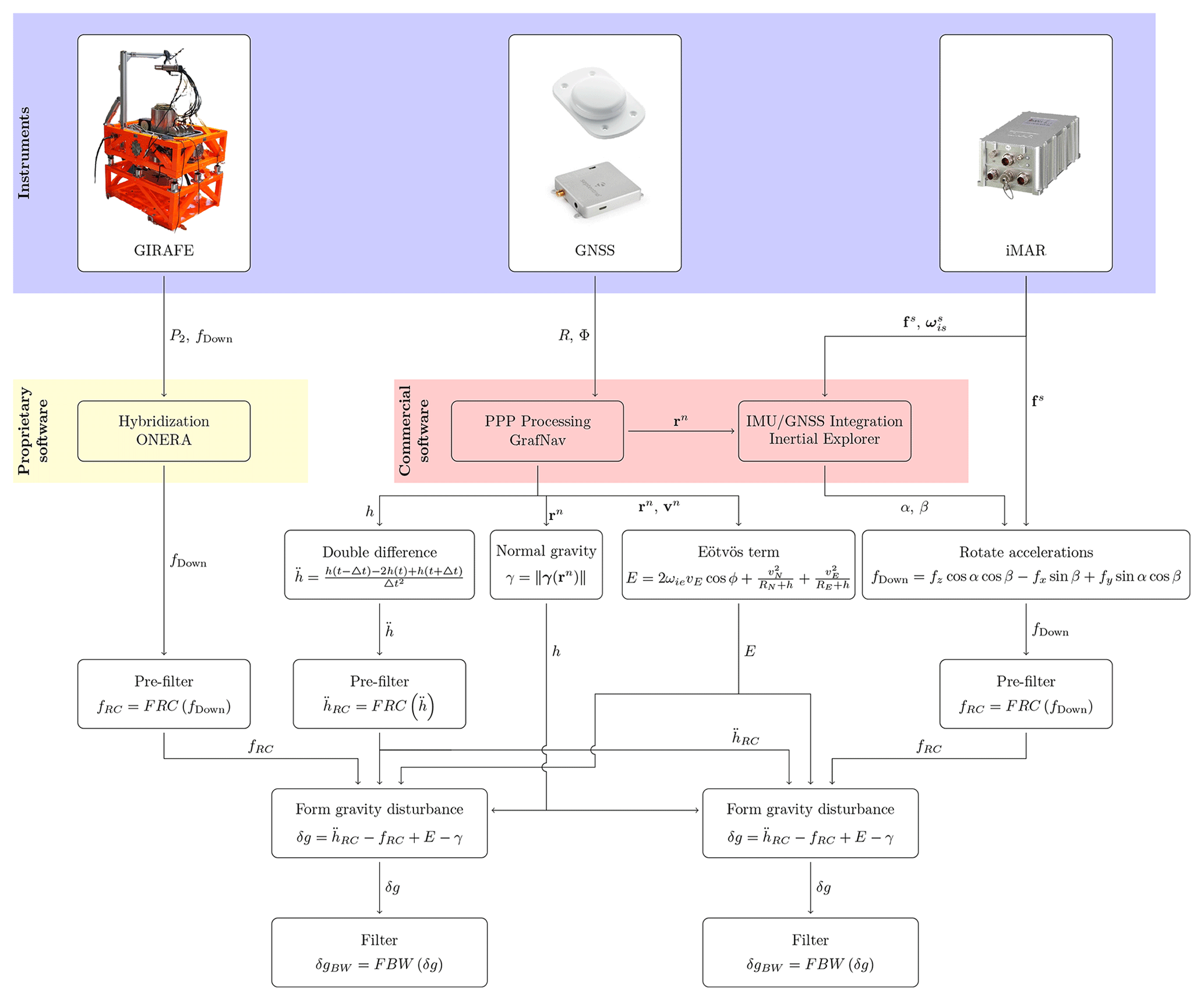
Figure 5 Processing flowchart. At the top are instruments generating raw observations in the form of probability P₂, vertical specific force f_Down, sensor frame specific force f^s, and sensor frame rotation rates ${\mathit{\omega }}_{is}^s$. Then follows initial processing using proprietary software to hybridise quantum observations for accelerations, f_Down, and commercial software to produce a pure GNSS-derived navigation solution, rⁿ and vⁿ, along with an integrated INS–GNSS solution for roll and pitch angles α and β. Following these initial steps, all variables are acquired to perform the processing described in Sect. 3.2.

The processing strategy applied here is similar to the one described in Johann et al. (2019) and focuses on scalar gravimetry, meaning that only the vertical component of Eq. (5) will be used, i.e.

$$\begin{array}{}\text{(6)}& {\displaystyle }\begin{array}{rl}\mathit{\delta }g=& \ddot{h}-f_{\text{Down}}+E-\mathit{\gamma }\\ =& \ddot{h}-f_{\text{Down}}+\mathrm{2}{\mathit{\omega }}_{ie}{v}_{\mathrm{E}}\cos \mathit{\varphi }\\ & +{\displaystyle \frac{v_{\mathrm{N}}^{\mathrm{2}}}{R_{\mathrm{N}}+h}}+{\displaystyle \frac{v_{\mathrm{E}}^{\mathrm{2}}}{R_{\mathrm{E}}+h}}-\mathit{\gamma },\end{array}\end{array}$$

where h is the ellipsoidal height, f_Down is the vertical component of a specific force, ω_ie is Earth's rotation rate, ϕ is the geodetic latitude, v_N and v_E are the northern and eastern velocities, and R_N and R_E are the Earth radii of curvature. The raw observations from the instruments are not directly the terms in the above expression. We must therefore first apply some pre-processing steps as indicated in Fig. 5, which is done using proprietary or commercial software products.

For the raw GNSS observations, the Waypoint commercial post-processing software suite from Hexagon or NovAtel is used to derive two data products:

1. A pure GNSS trajectory, $\mathit{r}=(\mathit{\varphi },\mathit{\lambda },h)$, based on a precise point positioning (PPP) processing strategy. The final satellite ephemeride products made available by the International GNSS Service (IGS) are utilised. More specifically, the 5 s clock products and 30 s orbit products from the Center for Orbit Determination in Europe (CODE) are used.

2. The GNSS-based PPP solution is merged with the iMAR iNAT-RQH accelerations and angular rates to derive an integrated IMU–GNSS navigation solution consisting of attitude, velocity, and position estimates. From these, the roll and pitch angles (α and β) along with the northern and eastern velocities (v_N and v_E) are needed in the processing chain.

From the GNSS-based PPP solution, the ellipsoidal height is numerically double-differentiated to obtain the kinematic acceleration $\ddot{h}$. It is important not to use height estimates from the integrated IMU–GNSS solution to obtain these accelerations. For all other terms in Eq. (6), the integrated solution can be used.

The roll and pitch angles of the integrated solution are used to project the specific force accelerations, $(f_x,f_y,f_z)$, measured by the iMAR strapdown gravimeter onto the vertical axis as (Glennie et al., 2000)

$$\begin{array}{}\text{(7)}& {\displaystyle }{\displaystyle }{f}_{\text{Down}}=f_z\cos \mathit{\alpha }\cos \mathit{\beta }-f_x\sin \mathit{\beta }+f_y\sin \mathit{\alpha }\cos \mathit{\beta },\end{array}$$

noting that a temperature drift correction has been applied to the vertical accelerometer as described in Becker et al. (2015).

The raw observations of the GIRAFE quantum gravimeter consist of a transition probability from the cold-atom interferometer and a specific force obtained from a Honeywell Quartz Accelerometer (QA) located below the vacuum chamber (Lawrence, 1998). These two observations are merged in a hybridisation algorithm described in Bidel et al. (2018) to arrive at a specific force, f_Down, which is measured directly along the vertical direction due to the mechanical platform. In other words, the mechanical platform ensures that $\mathit{\alpha }=\mathit{\beta }=\mathrm{0}$, such that f_Down=f_z.

Finally, before proceeding, these observables, f_Down and $\ddot{h}$, are subjected to an initial filter with a kernel width of 1 to 2 s. During processing this was seen to remove some error effects and produce more consistent results between the various solutions. For this, an implementation of a resistor–capacitor (RC) circuit low-pass filter was employed. The process is denoted as FRC in Fig. 5.

Following these pre-processing steps, we obtain all the terms in Eq. (6), allowing us to compute the gravity disturbance. It should be noted that the specific force, f_Down, can be derived from either the GIRAFE quantum gravimeter or the iMAR iNAT-RQH gravimeter, and the kinematic acceleration term, $\ddot{h}$, can be derived from any of the three GNSS receivers on board the aircraft. The expected gravity signal variation at altitude is typically of the order of 10 mGal, whereas the observation noise in f_Down and $\ddot{h}$ is typically of the order of 10⁵ mGal, meaning that a heavy low-pass filter must be applied in order to reduce high-frequency noise in the observations. For this dataset, the final gravity estimates are supplied both non-filtered and at three different filter lengths. The applied low-pass filter is a zero-phase second-order Butterworth filter with filter width specified in terms of the full width half maximum (FWHM) of the kernel (Jensen, 2022).

3.3 External gravity observations

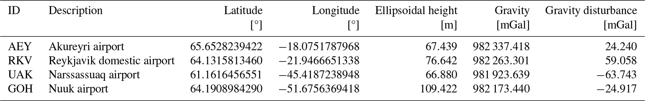
Following the processing described in the previous section, the relative gravity disturbance estimates derived from the iMAR strapdown sensor need to be corrected for the systematic errors contained therein. External gravity observations, known as tie values, are performed on the apron next to the aircraft parking position. Comparing these tie values with the gravity estimates before and after flight, while the aircraft is stationary on the apron, allows for the estimation of an offset and linear trend, which is used to correct the gravity estimates. The tie values used for this correction are listed in Table 2. Note that the GIRAFE gravity sensor is not subject to such systematic errors and thus requires no tie value correction.

Table 2 External gravity observations used as tie values to estimate the bias and trend of the gravity estimates derived using the iMAR strapdown gravimeter. All the gravity values refer to the ground level on the apron and are listed as gravity vector magnitude and gravity disturbance. Coordinates are geodetic with respect to the WGS84 ellipsoid.

3.4 Internal cross-over evaluation

As a means of internally evaluating the precision of the obtained results, gravity estimates at the same point in space resulting from two different flight segments can be compared. As illustrated in Fig. 6, the airborne survey is typically designed as parallel flight tracks with perpendicular tie lines for evaluating the survey. At the points in space where the lines cross, two estimates of the gravity value are available and can be compared. If a considerable number of such cross-over points are available, it is possible to derive some statistics from the differences as illustrated in Fig. 6. The most commonly quoted value is the root mean square error (RMSE), defined as

$$\begin{array}{}\text{(8)}& {\displaystyle }{\displaystyle }\text{RMSE}={\displaystyle \frac{\text{RMS}}{\sqrt{\mathrm{2}}}}=\sqrt{{\displaystyle \frac{\mathrm{1}}{\mathrm{2}N}}\stackrel{N}{\sum _{n=\mathrm{1}}}}{\mathit{ϵ}}_i^{\mathrm{2}},\end{array}$$

where ϵ_i denotes the cross-over difference and N is the total number of crossing points. The RMSE value is typically associated with the survey accuracy.

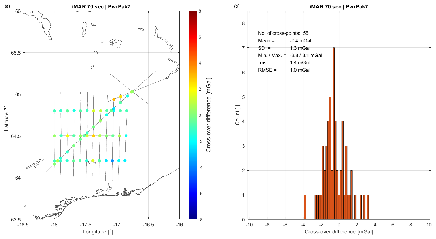
Figure 6 Illustration of the cross-over error evaluation over the Vatnajökull ice cap. The figure title indicates the gravimeter (iMAR), GNSS receiver (PwrPak7), and filter width (70 s). (a) Cross-over differences in estimated gravity values from the two crossing flight lines. (b) Histogram derived from the cross-over differences. Also shown are the statistics derived from the differences.

It should be noted that crossing flight lines may not be carried out at the same flight altitude. Since the normal gravity field is removed from the full gravity magnitude, a vertical variation corresponding to that of the GRS80 normal gravity field is accounted for. In practice, the vertical variation may differ from that of the model, and care must be exercised when comparing estimates obtained at significantly different heights.

3.5 Comparison with other gravity observations

Another independent evaluation compares new gravity observations with existing gravity observations in the area. Generally, these observations are collected at sea, on land, on ice, and in the air, meaning that they must be interpolated and extrapolated both horizontally and vertically in order to evaluate new observations. Both Iceland and Greenland have numerous sources of gravity anomaly data in the joint Nordic gravity database, both onshore and offshore. Although many land data sources date back to the 1950s, all data have been rectified and quality-checked according to modern gravity standards and quality-checked extensively in connection with recent Greenland and Iceland Geoid projects. Since the existing data are available in the form of gravity anomalies, △g, rather than gravity disturbances, δg, used in this paper, the upward continued ground data are converted into gravity disturbances.

The upward continuation process has been carried out by fast Fourier transformation in a remove–restore process, taking into account both the Global Gravity Model (GGM) and terrain effects. The GRAVSOFT suite of programs (Forsberg and Tscherning, 2014) has been used in this process in the following steps:

1. Reduction of the gravity anomalies, △g, by computing a reference field, △g_N180, using the EIGEN-6C4 model to degree and order 180 (Förste et al., 2014) and forming the residuals (GRAVOSFT geocol17):

   $$\begin{array}{}\text{(9)}& {\displaystyle }{\displaystyle }\mathrm{△}{g}_{\text{GGM}}=\mathrm{△}g-\mathrm{△}{g}_{\text{N180}}.\end{array}$$

2. Removing the short-wavelength topographic effects using residual terrain modelling (Forsberg, 1984) by computing the gravitational attraction, △g_DEM, from topography, bathymetry, and ice mass using prism integration (GRAVOSFT TC):

   $$\begin{array}{}\text{(10)}& {\displaystyle }{\displaystyle }\mathrm{△}{g}_{\text{GGM}+\text{DEM}}=\mathrm{△}{g}_{\text{GGM}}-\mathrm{△}{g}_{\text{DEM}}.\end{array}$$

3. Gridding the reduced gravity data on a regular grid using least-squares collocation (GRAVOSFT GEOGRID) with a planar-logarithmic covariance model (Forsberg, 1987) and then upward-continued gravity data to flight altitudes (GRAVOSFT GEOFOUR), taking into account the differing flight elevations using 3D “sandwich” interpolation between several flight levels:

   $$\begin{array}{}\text{(11)}& {\displaystyle }{\displaystyle }\mathrm{△}{g}_{\text{GGM}+\text{DEM}}^H=\text{FFT}\left[\mathrm{△}{g}_{\text{GGM}+\text{DEM}}\right].\end{array}$$

4. Restoring the GGM and terrain effects at the flight altitudes (GRAVSOFT TC and GEOCOL17) and converting the upward-continued gravity anomalies into gravity disturbances:

   $$\begin{array}{ll}{\displaystyle }\mathit{\delta }{g}^H=& {\displaystyle }\mathrm{△}{g}_{\text{GGM}+\text{DEM}}^H+\mathrm{△}{g}_{\text{DEM}}^H\\ \text{(12)}& {\displaystyle }& {\displaystyle }+\mathrm{△}{g}_{\text{N180}}^H+\mathrm{0.3086}\cdot N,\end{array}$$

   where 0.3086 mGal m⁻¹ is the vertical gradient of gravity and N is the geoid undulation, i.e. the height of the geoid above the ellipsoid.

Following these steps, the computed gravity disturbances are mildly filtered to match approximately the inherent along-track filtering in the airborne data.

3.5.1 Iceland

The gravity data of Iceland cover the ice-free land areas, the major glaciers, and numerous sources offshore, as illustrated in Fig. 7. The DEM and gravity data in the database of the Nordic Geodetic Commission (NKG) were provided by Landmælingar Islands (Iceland Geodetic Survey), with data on the ice, including radar echo sounding of ice thickness, provided by the University of Iceland. The terrain effect computations assume a rock density of 2.67 g cm⁻³ and an ice density of 0.92 g cm⁻³. The land DEM of Iceland is based on 2 arcsec resolution data, while no bathymetry data were used. The Geoid model used for anomaly–disturbance correction is based on the latest Iceland Geoid model (Forsberg and Valsson, unpublished). Due to the relatively dense gravity data coverage around the flight tracks, the errors of the upward-continued gravity disturbances are estimated at 2–3 mGal based on residuals from least-squares collocation.

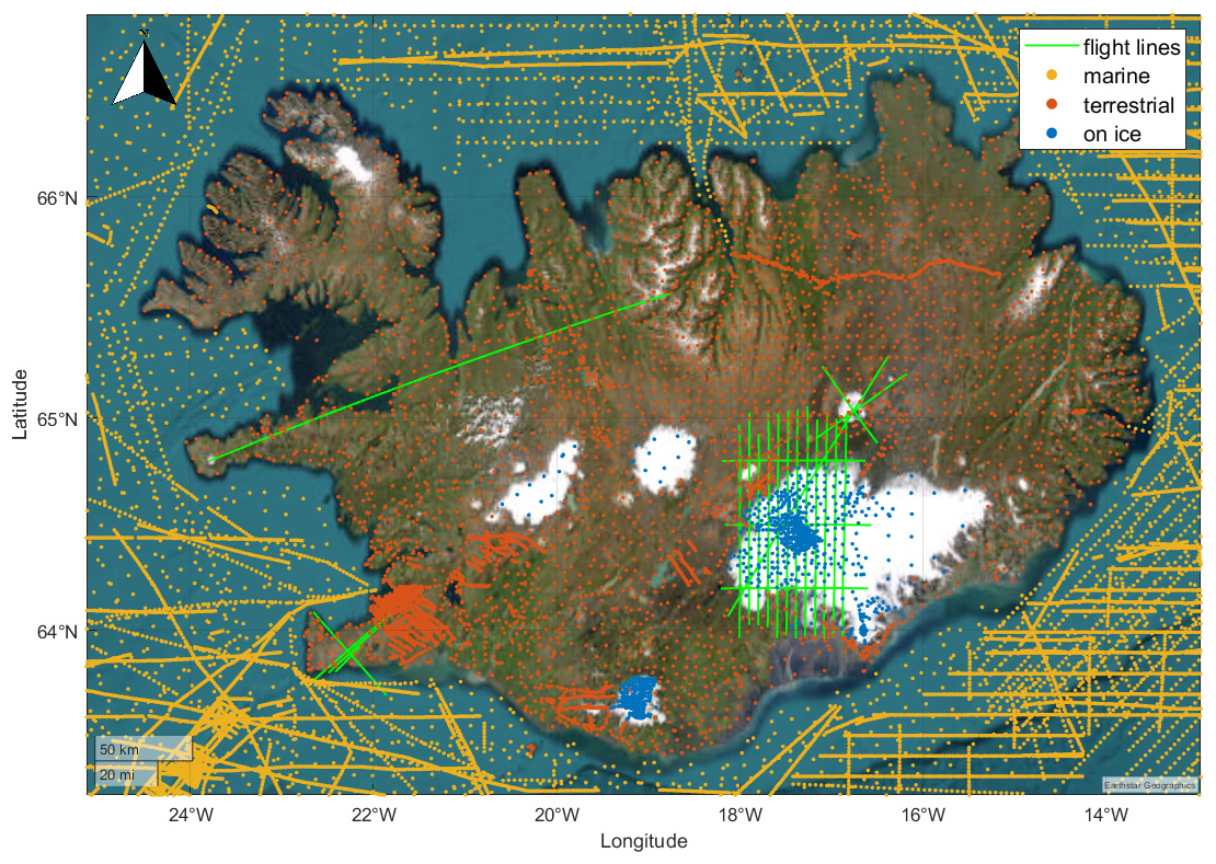
Figure 7 Illustration of existing gravity data in Iceland along with the flight lines of the current campaign.

3.5.2 Nuuk

In the Nuuk fjord system, large fjords, many of them unsurveyed, have depths well in excess of 1000 m, meaning that the fjords themselves generate narrow gravity anomalies of up to 60–80 mGal that are not captured well by the 1960s' numerous land gravity points along the fjords. With the lack of fjord depths, the sparse bathymetry available was not used, but instead existing high-altitude airborne gravity data from the US Naval Research Lab 1991/92 (Brozena, 1992), data from Operation IceBridge (2009–2012), and low-level airborne data from DTU Space (2003–2007) along the offshore region were used. To utilise all of the data together, advantage was taken of the 2016 Greenland Geoid model (GGEOID16, Forsberg and Jensen, 2016; International Service for the Geoid, http://www.isgeoid.polimi.it, last access: 14 April 2025). Here all gravity data available in Greenland and the surrounding oceans were combined in a rigorous downward continuation to the surface, using blocked least-squares collocation (GRAVSOFT gpcol) and taking into account the different accuracies and elevations of the various data sources. The GGM was EIGEN-6C4 as in Iceland, with DEM surface data taken from Byrd Polar Research Center (BPRC 2013) from optical imagery downsampled to 500 m resolution, with ice thickness from Bamber et al. (2001) regridded to the DEM spacing. Due to the lack of airborne radar data over the margins of the Greenland ice sheet, the ice thickness model has large errors here (of less importance for the Nuuk flight region). For the intercomparison with the airborne gravity data presented in this paper, the downward-continued gravity anomaly grid at 2 km resolution from the GGEOID16 computation continued upward to the 2023 flight elevations and was converted into gravity disturbance. The data coverage underlying GGEOID16 is shown in Fig. 8.

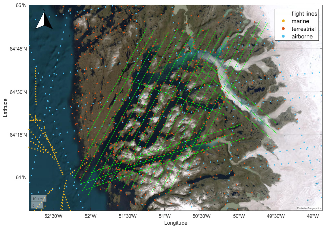
Figure 8 Illustration of existing gravity data in the Nuuk area along with the flight lines of the current campaign.

3.6 Combining estimates from two sensors

In the “Results and discussion” section there will be indications of increased spatial coverage and resolution from the iMAR strapdown sensor, while the GIRAFE system shows superior results in terms of stability. As these properties are complementary, this motivates a combination of the two sensors. An in-depth study of the hybridisation of these sensors is beyond the scope of this paper, but a simple combination approach will be used to illustrate the potential and some characteristics of the data.

The combination is performed on a line-by-line basis by forming the fast Fourier transform (FFT) of the estimates coming from each instrument. This leads to two sets of coefficients:

$$\begin{array}{}\text{(13)}& {\displaystyle }\begin{array}{rl}{\displaystyle }& {\displaystyle }{X}_k^{\text{iMAR}}=\mathrm{FFT}\left[\mathrm{d}{g}^{\text{iMAR}}\left(x\right)\right],\\ {\displaystyle }& {\displaystyle }{X}_m^{\text{GIRAFE}}=\mathrm{FFT}\left[\mathrm{d}{g}^{\text{GIRAFE}}\left(x\right)\right],\end{array}\end{array}$$

where $k=\mathrm{0},\mathrm{1},\mathrm{\dots },K$ and $m=\mathrm{0},\mathrm{1},\mathrm{\dots },M$ are the number of coefficients for each gravity profile and x refers to the along-track distance. In order to retain the high-frequency information (spatial variability) from the iMAR instrument and the low-frequency information (stability) from the GIRAFE instrument, we can use the low-degree coefficients from GIRAFE and higher-degree coefficients from iMAR. We may therefore form a new set of coefficients

$$\begin{array}{}\text{(14)}& {\displaystyle }\begin{array}{rl}{X}_n^{\text{comb}}=\mathit{\{}& X_{\mathrm{0}}^{\text{GIRAFE}},X_{\mathrm{1}}^{\text{GIRAFE}},X_{\mathrm{2}}^{\text{GIRAFE}},\mathrm{\dots },\\ & X_N^{\text{GIRAFE}},X_{N+\mathrm{1}}^{\text{iMAR}},X_{N+\mathrm{2}}^{\text{iMAR}},\mathrm{\dots },X_K^{\text{iMAR}}\mathit{\}},\end{array}\end{array}$$

from which we can restore the gravity profile using an inverse FFT to arrive at a combined estimate:

$$\begin{array}{}\text{(15)}& {\displaystyle }{\displaystyle }\mathrm{d}{g}^{\text{comb}}\left(x\right)=\mathrm{iFFT}\left[X_n^{\text{comb}}\right].\end{array}$$

The amount of information retrieved from the GIRAFE and iMAR estimates can be varied by changing the degree, N, indicating the number of coefficients used from the GIRAFE estimates.

4 Results and discussion

This section aims to give a brief overview of the results and point out some key points. The results will be divided into four sections defined by geographical location.

4.1 Vatnajökull ice cap and Askja volcano

Gravity estimates over the Vatnajökull ice cap are illustrated in Fig. 9. To the north-east of the ice cap is the Askja volcano, which has been associated with significant vertical displacement (Pagli et al., 2006). Two sets of gravity estimates are illustrated, one derived using the GIRAFE quantum instrument and one derived using the iMAR strapdown gravimeter. From the figure it is evident that the iMAR dataset has a better spatial coverage than the GIRAFE dataset (2337 line kilometres vs. 2183 line kilometres, i.e. 7 % more). This is the result of a subjective process where some data are discarded by the person processing the data, which is mostly related to aircraft turns but can also be a result of turbulence or other artefacts. The improved spatial coverage was observed previously and is most likely related to the mechanical platform rather than the sensor technology (Jensen et al., 2019). On the other hand, the platform has also been seen to provide better long-term stability of measurements.

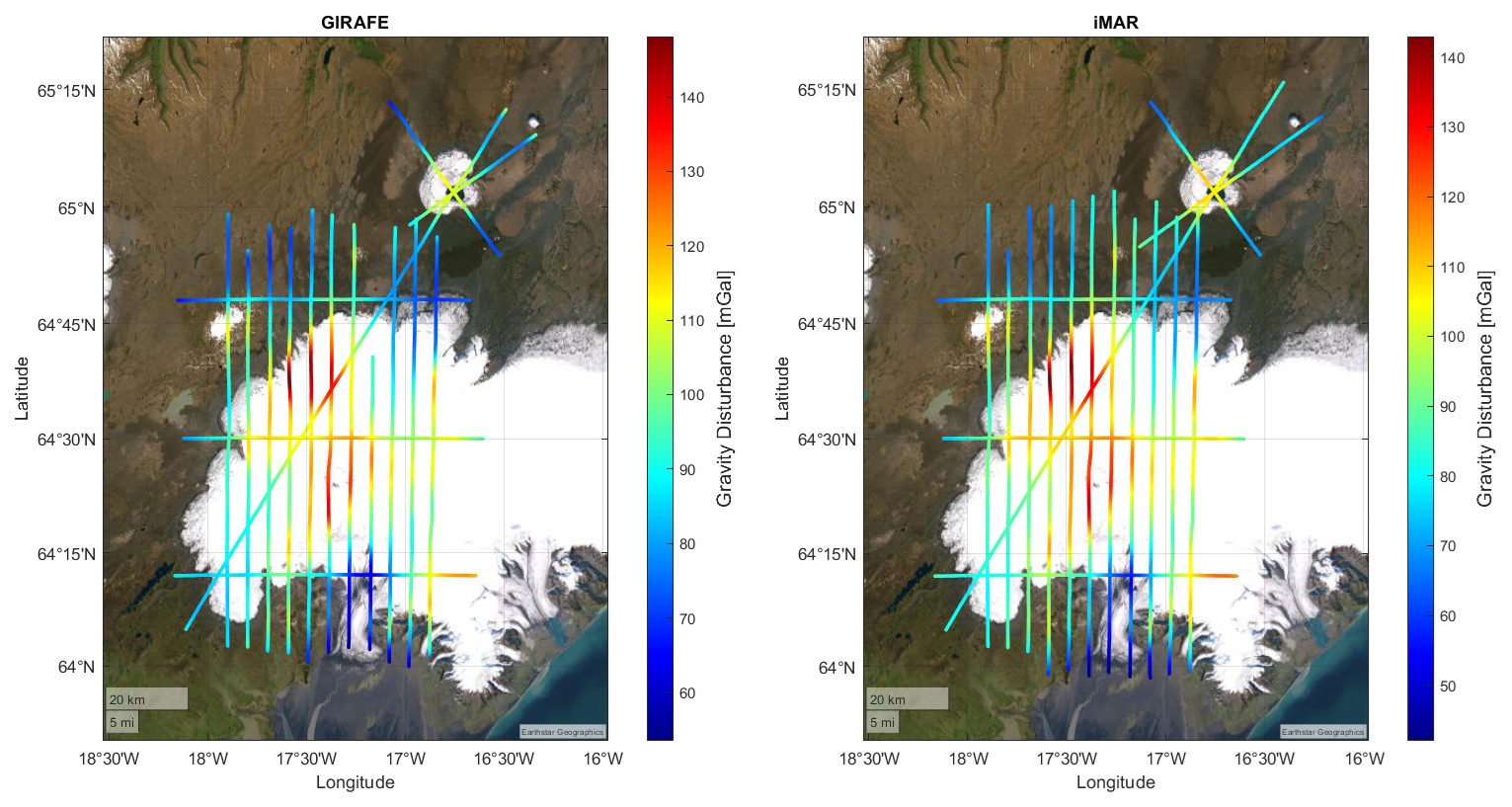
Figure 9 Gravity disturbance estimates from the Vatnajökull ice cap and the Askja volcano. Kinematic accelerations are derived from the NovAtel PwrPak7 GNSS receiver and disturbance estimates are low-passed-filtered using a FWHM filter width of 70 s. (a) Estimates derived from GIRAFE. (b) Estimates derived from iMAR.

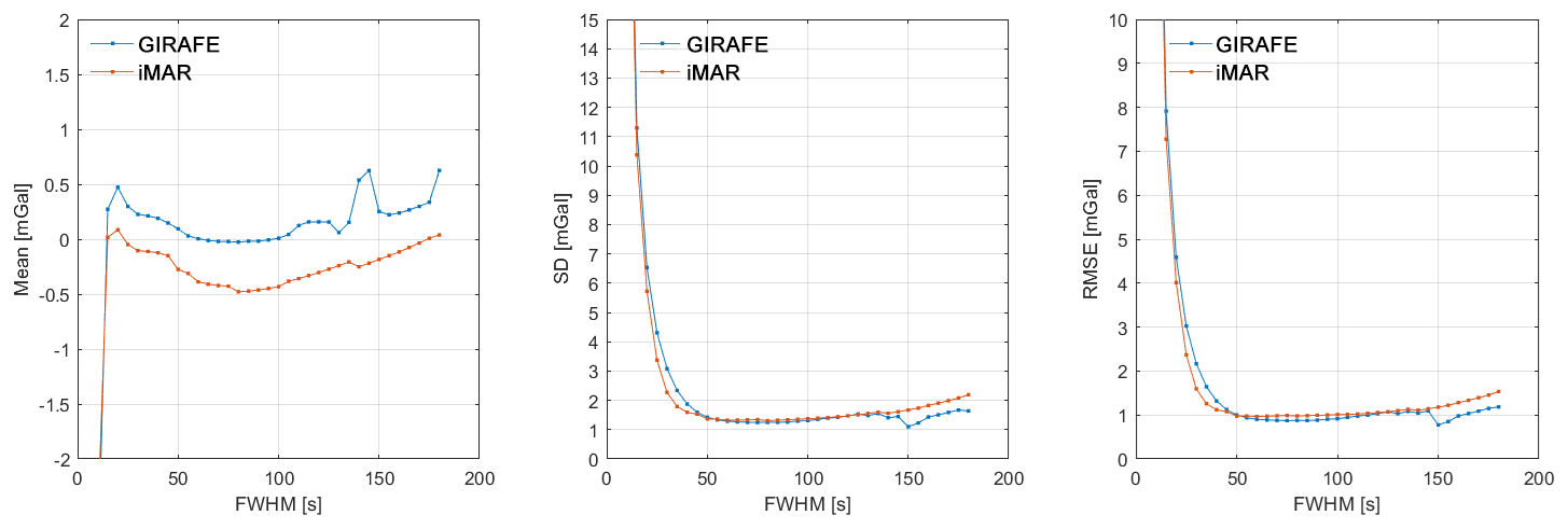
Figure 10 Mean, standard deviation, and RMSE of the cross-over differences as a function of filter width at the Vatnajökull ice cap and the Askja volcano.

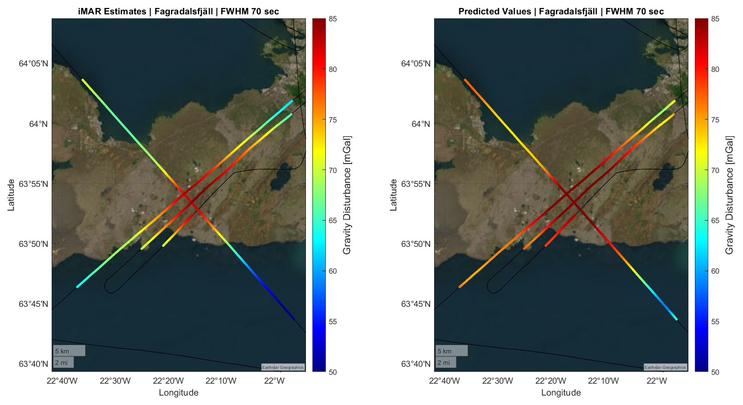
Figure 11 Gravity disturbance estimates from (a) the iMAR strapdown sensor from a new airborne survey and (b) predicted gravity disturbance from previous gravity observations.

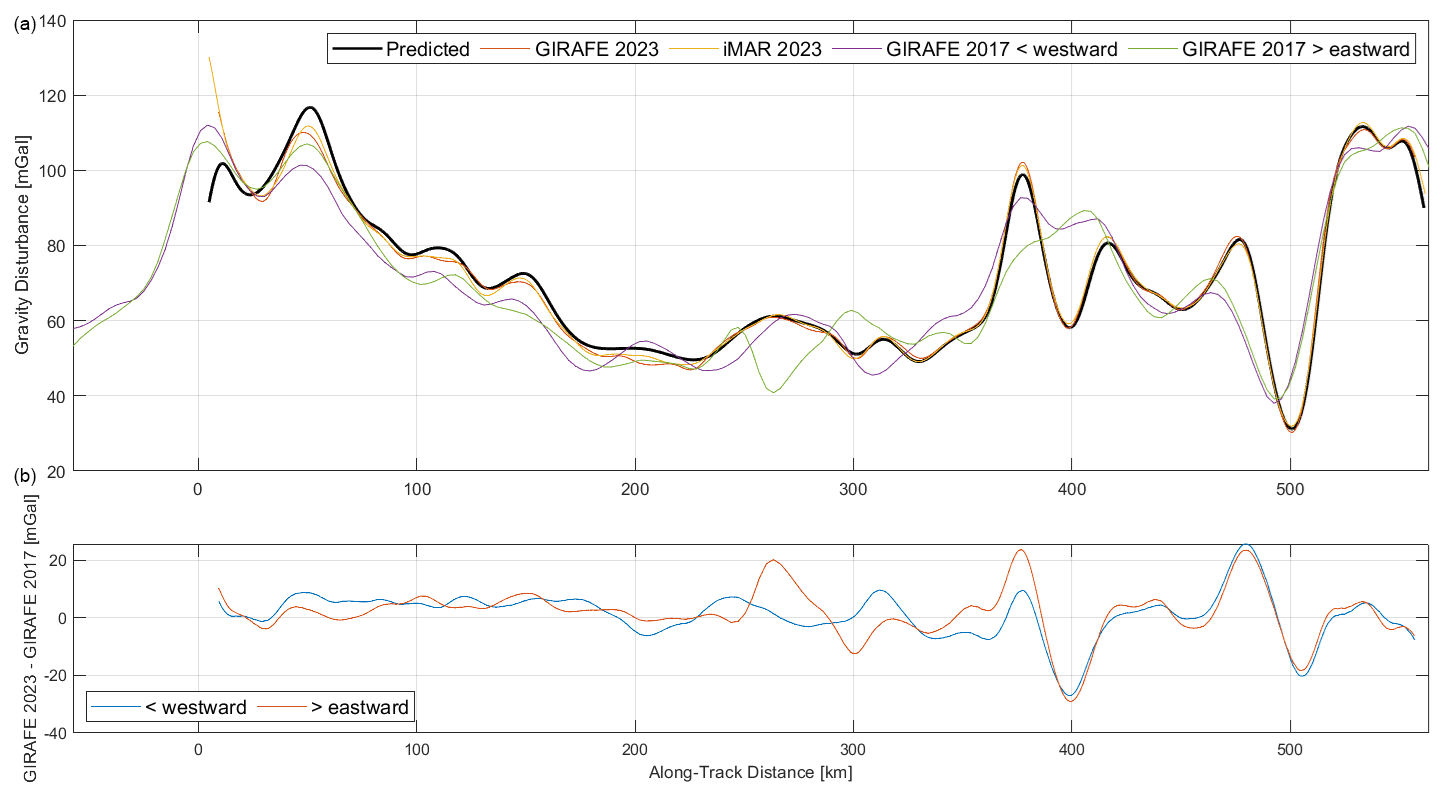
Figure 12 Gravity disturbance estimates along the flight line from Snæfellsjökull to Akureyri. Note that this line was flown once from west to east during the campaign in 2023, while it was flown twice during the campaign in 2017. (a) Predictions from existing observations (black), from GIRAFE 2023 (red), from iMAR 2023 (yellow), and from GIRAFE 2017 (purple and green). (b) Difference between GIRAFE estimates in 2023 and 2017.

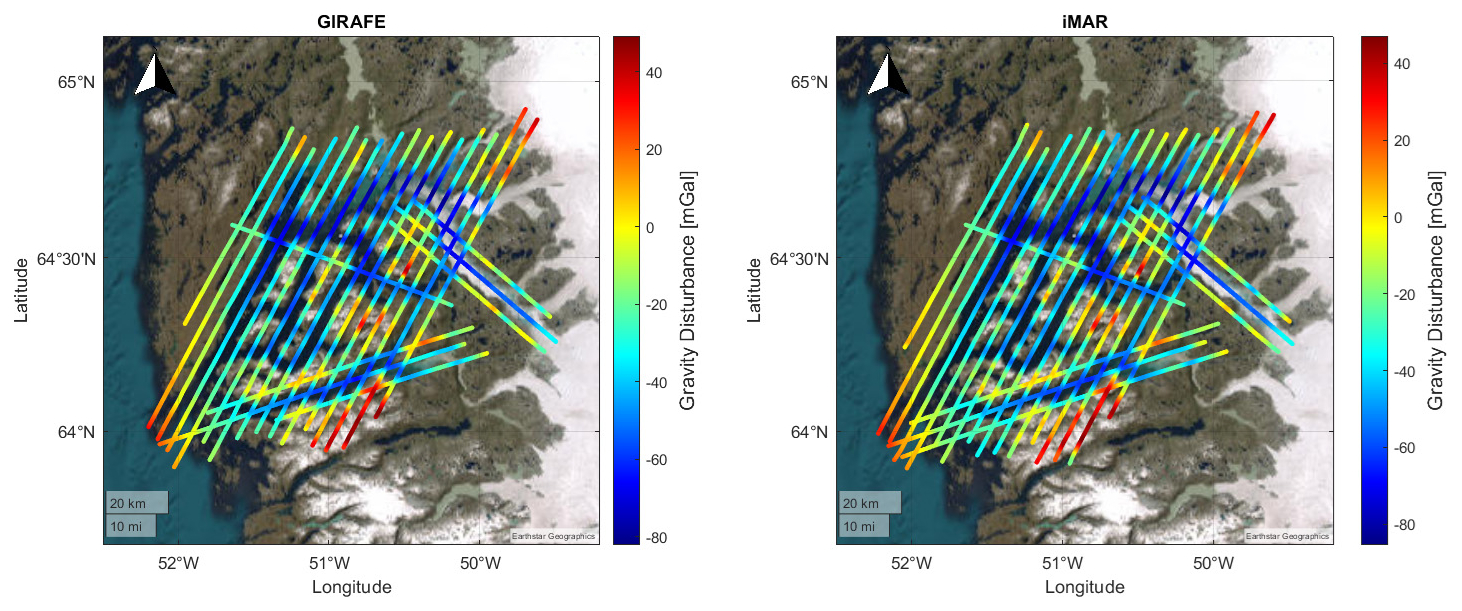
Figure 13 Gravity disturbance estimates from the Nuuk fjord system. Kinematic accelerations are derived from the NovAtel PwrPak7 GNSS receiver and disturbance estimates are low-passed-filtered using a FWHM filter width of 40 s. (a) Estimates derived from GIRAFE. (b) Estimates derived from iMAR.

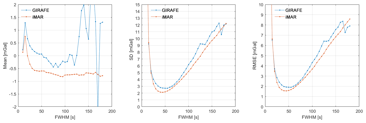
Figure 14 Mean, standard deviation, and RMSE as a function of filter width derived from cross-over differences in the Nuuk fjord system. Note that, as the filtering increases, fewer cross-over points become available, leading to unstable statistics.

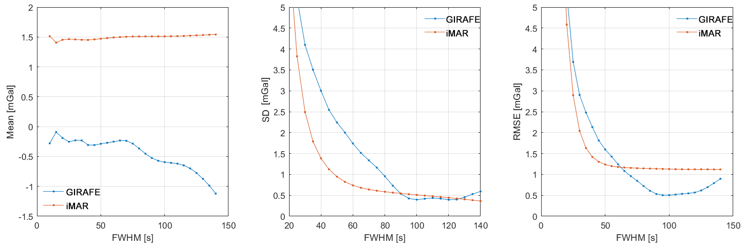
Figure 15 Mean, standard deviation, and RMSE as a function of filter width derived from differences between two repeats of the east–west tie line crossing all the north–south parallel lines.

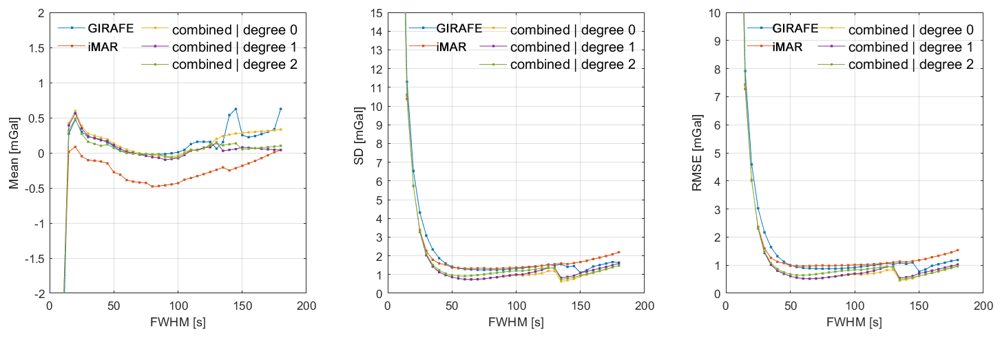
Figure 16 Mean, standard deviation, and RMSE values derived from cross-over differences at the Vatnajökull ice cap. These statistics are derived as a function of filtering for GIRAFE estimates (blue), iMAR estimates (red), and a combination of the two instruments. The three different variants represent results using only the zero-degree term from GIRAFE (yellow); the zero- and first-degree terms from GIRAFE (purple); and the zero-, first-, and second-degree terms from GIRAFE (green).

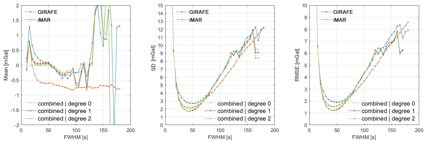
Figure 17 Mean, standard deviation, and RMSE values derived from cross-over differences in the Nuuk fjord system. These statistics are derived as a function of filtering for GIRAFE estimates (blue), iMAR estimates (red), and a combination of the two instruments. The three different variants represent results using only the zero-degree term from GIRAFE (yellow); the zero- and first-degree terms from GIRAFE (purple); and the zero-, first-, and second-degree terms from GIRAFE (green).

The two datasets in Fig. 9 are not unique. They are derived using one of the three available GNSS receivers. Furthermore, the results depend on the final low-pass filter applied to the gravity disturbance estimates. As a way of objectively investigating the optimal amount of filtering, some statistical measures can be derived from the cross-over differences using several values of the filter width (full width half maximum). Such an analysis was carried out in Fig. 10, indicating that a value of around 70 s for the FWHM provides optimal results, with an accuracy of around 1 mGal for both systems in terms of the RMSE value.

Interpretation of the mean value in the left panel in Fig. 10 is not straightforward. However, if systematic errors, other than a constant offset, are present in the data, such errors would lead to non-zero mean values. The figure may therefore be an indication of the improved stability of the GIRAFE quantum instrument, while significant systematic errors may be present for the iMAR strapdown instrument.

4.2 Fagradallsfjall volcano

The Fagradallsfjall volcano, situated only 35 km from Keflavik International Airport, has seen a number of recent eruptions, with one occurring just a few days after our survey (Halldórsson et al., 2022; Sigmundsson et al., 2022). Such volcanic eruptions indicate a direct re-distribution of mass that will affect the associated gravity field. Figure 11 illustrates both the measured and predicted gravity values along the flight lines of the current campaign.

Although the orders of magnitude are the same and some spatial patterns correlate, it is difficult to directly compare the two signals. Inspecting Fig. 7, it is evident that the spatial coverage of previous observations is relatively poor in the area. As a result, the detailed signal is mostly dictated by the DEM used for the area, which again may not be accurate since the topography has actively changed due to deposition of lava on the surface. These newly acquired data may thus provide useful information in future studies of mass transportation related to volcanic activity in the area.

4.3 Flight line from Snæfellsjökull to Akureyri

During the previous flight campaign in 2017, a flight line between Akureyri and Snæfellsjökull was surveyed from westward and eastward using the GIRAFE instrument; see Bidel et al. (2020). During the 2023 campaign this survey line was flown again during transit from Greenland back to Akureyri. The resulting gravity estimates are shown in Fig. 12 along with the estimates from the 2017 campaign and those predicted from the existing gravity observations.

The figure shows that the new gravity estimates correlate quite well with the predicted estimates, although some significant differences are apparent during the first 250 km of the line. Again, referring to Fig. 7, it is evident that this correlates with poor data coverage only north of the parallel mountain ridge and the crossing of a fjord with no associated data.

The bottom figure shows the difference from the 2017 campaign, which was the first ever flight test of the quantum gravimeter. This figure is an indication of the improvement that the instrument has undergone during those 6 years of development.

4.4 Nuuk fjord system

Gravity estimates from the Nuuk fjord system are shown in Fig. 13. By comparing the GIRAFE and iMAR datasets, it is again evident that the strapdown system results in a superior spatial coverage (3795 line kilometres vs. 3560 line kilometres, i.e. 7 % more). The mean, standard deviation, and RMSE values derived from cross-over differences are shown in Fig. 14, indicating an accuracy of around 1.5–2.0 mGal in terms of RMSE and an optimal value of 40 s for the filter FWHM.

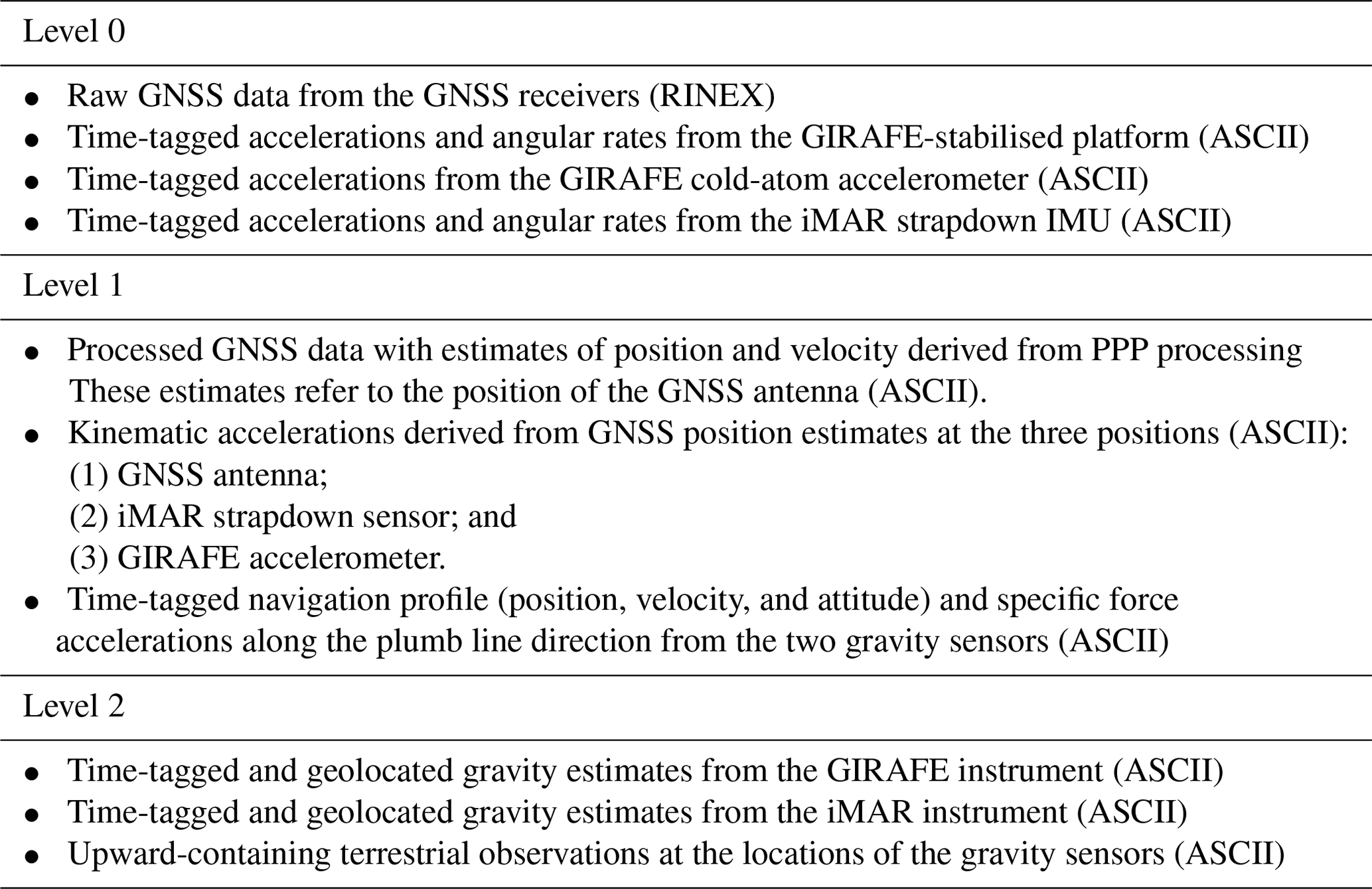
Table 3 Description of the data products made available from the campaigns.

It is generally expected that noise will attenuate with filtering, such that more filtering leads to better results. However, the filtering not only removes noise but also smooths out the actual gravity signal as the aircraft moves along its path. This means that the derived gravity estimate represents an average gravity value along the aircraft trajectory, depending on the shape of the filter kernel and the filter width. In a cross-over analysis, the flight lines are not parallel, meaning that gravity estimates represent averages over different trajectories in space. For this reason, the derived RMSE value is expected to increase when the error induced by smoothing the signal along different directions becomes larger than the noise reduction due to filtering. An alternative to cross-over validation is to repeat the same line segment twice. In Nuuk, this was done with the east–west tie line crossing the 16 north–south-oriented parallel lines; this was flown twice. In this case we can directly form the difference in gravity estimates along the line and derive statistics similar to the cross-over differences. This is shown in Fig. 15.

Inspection of the mean value in Fig. 15 indicates a small offset between the GIRAFE estimates, while a significant offset is present for the iMAR estimates. The standard deviation and RMSE values are seen to generally decrease as a function of more filtering. As argued above, this is as expected. One twist is that erroneous estimates from aircraft turns will increasingly propagate into the straight-line segments with increased filtering. This is handled by removing more and more from the beginning and end of a line. As a result, the length of the line that can be compared decreases with increased filtering.

The filtering will also not remove systematic errors such as bias. This is evident from comparing the standard deviation and RMSE values for the iMAR estimates. Since the standard deviation accounts for a mean value, this value drops to around 0.5 mGal, while the RMSE value flattens out at around $\mathrm{1.5}/\sqrt{\left(\mathrm{2}\right)}\approx \mathrm{1.1}$ mGal, corresponding to the mean difference of 1.5 mGal.

Comparing Fig. 14 with Fig. 10 indicates that less filtering is required in Nuuk before the errors induced by spatial filtering surpass the noise reduction from filtering. Theoretically, this is in line with expectations since the gravity field in Nuuk varies much more in terms of magnitude and distance compared with the Vatnajökull ice cap. This is a direct consequence of the topography resulting from deep fjords and steep mountain slopes.

4.5 Combining estimates from two sensors

To illustrate the potential of hybridising the two sensor technologies, the simple combination strategy presented in Sect. 3.6 is used to arrive at combined estimates. Although the methodology used here is not directly relevant for future satellite missions, the combination indicates some potential benefits of a hybridisation strategy. Figures 16 and 17 show the mean and RMSE values derived from a combination of the two instruments. The blue and red curves are the same as those presented in Figs. 10 and 14.

The two figures illustrate that the combination works according to the intention. First of all, the mean values of the GIRAFE estimates are adopted, whereas the lower standard deviations of the iMAR estimates are adopted. As a result, the combined accuracy in terms of RMSE decreases to around 0.5 mGal for Vatnajökull and 1.2 mGal for Nuuk. Additionally, we can see that no improvement follows from using more than the zero-degree term from the GIRAFE estimates. This may indicate that the iMAR estimates are subject to a line-by-line bias error.

5 Data availability

The data from the two campaigns are made available on the ESA Earth Online webpage (Jensen et al., 2024, https://doi.org/10.57780/esa-58c58c5). The data are divided into raw, intermediate, and final data products, depending on the level of post-processing applied. An overview is given in Table 3. A more elaborate description of the data products and format can be found in the associated ESA report and the README files distributed along with the data.

6 Conclusions

This paper presents a dataset obtained from an airborne gravity campaign covering the Vatnajökull ice cap along with two volcanic targets in Iceland and the Nuuk fjord system in Greenland. The instrumentation includes the GIRAFE cold-atom gravity sensor and the iMAR iNAT-RQH strapdown gravity sensor, along with three different GNSS receivers. The data from the campaign are made available in three categories, depending on the amount of post-processing applied. See the “Data availability” section. This should enable anyone to use the data, whether they are interested in investigating processing techniques or using the data for geophysical studies.

Following an overview of the survey and instrumentation, the processing strategy applied to derive the level-1 and level-2 data products is presented in the paper. Finally, some results are presented in order to describe the characteristics of the data and to show the potential for using the data in geophysical studies.