Features of Italian large dams and their upstream catchments

In Italy, a complete and updated database including the most relevant structural information regarding reservoirs and characteristics of their upstream watersheds is currently missing. This paper tackles this gap by presenting the first comprehensive dataset of 528 large dams in Italy. Alongside structural details of the dams, such as coordinates, reservoir surface area and volume, the dataset also encompasses a range of geomorphological, climatological, extreme rainfall, land cover and soil-related attributes of their upstream catchments. The data used to create this dataset are partially sourced from the General Department of Dams and Hydro-Electrical Infrastructures as well as from the processing of updated and standardized grid data. These include a DEM from the Shuttle Radar Topography Mission, national-scale monthly maps of hydrological budget components, land cover and vegetation index data from the Copernicus Land Monitoring Service as well as high-resolution maps of soil particle size fractions. This dataset (Evangelista et al., 2024a; https://doi.org/10.5281/zenodo.12818297), which contains information not easily available in other similar global or national data collections, is expected to be of great help for a broad spectrum of hydrological applications, particularly those related to floods.

1 Introduction

Dams play an important role in managing water resources (Ehsani et al., 2017). Water storage through reservoirs becomes strategic to secure water resources for cities, agriculture and industrial activities during the most critical periods, when natural conditions are inadequate for meeting human water needs (Liu et al., 2018). Reservoirs' capacity to retain water volumes can also aid in mitigating downstream flood effects during severe meteorological events (Zhao et al., 2020; Boulange et al., 2021).

On the other hand, dams can significantly impact the natural flow regime of rivers (e.g. Tundisi, 2018; Barbarossa et al., 2020; Parasiewicz et al., 2023), and these effects may vary depending on the operational procedures employed (e.g. Annys et al., 2020) and the management practices at the catchment scale (e.g. Kondolf et al., 2018). The way dams are managed can lead to rapid and unnatural flow fluctuations, with consequences for downstream ecosystems (Greimel et al., 2018). Additionally, improper management of spillways can result in increased peak discharges in the downstream areas during flood events (Liu et al., 2017).

Proper management and maintenance of dams become crucial to ensuring their safe and efficient operation while minimizing any potential negative impacts, particularly as many of these structures, built in the first half of the 20th century, are now ageing. This involves addressing the complex inter-relationships between dams and their host environment. With this aim, knowing the exact locations of reservoirs, their ages, their primary uses, their structural features and the main characteristics of their upstream basins can help researchers and decision-makers better understand the potential risks and benefits associated with their operation on basin scales of various sizes (Speckhann et al., 2021).

In recent years, some research works have been conducted to obtain global-scale collections of data on these infrastructures; such initiatives aim to catalogue large dams worldwide, facilitating cross-country comparisons.

The first global-scale dataset was the Global Reservoir and Dam database (GRanD) (Lehner et al., 2011), developed within the Global Water System Project. GRanD contains information regarding more than 6800 dams and their associated reservoirs.

Later on, the GlObal geOreferenced Database of Dams (GOODD) (Mulligan et al., 2020) was released. GOODD is a global dataset of more than 38 000 georeferenced dams containing both their geographic coordinates and information on the associated catchment areas. Dams were digitized by scanning tiles on the Google Earth geobrowser (https://earth.google.com/web/, last access: 31 March 2025) using a GeoWiki coded in KML (Keyhole Markup Language). Catchment boundaries were derived from the HydroSHEDS SRTM-based DEM (Lehner et al., 2008) at 30 arcsec resolution for the latitudes from 60° N to 60° S, complemented by the Hydro1K DEM at 30 arcsec resolution for the remaining 30° amplitude bands at the poles. The GOODD and GRanD datasets are among those that constitute the recent river barrier and reservoir database developed under the Global Dam Watch (GDW) initiative (Lehner et al., 2024), which collects data on over 40 000 dam points worldwide.

Recently, Zhang and Gu (2023) released the GDAT (Global Dam Tracker) dataset containing more than 35 000 reservoirs all over the world, where dam coordinates are verified using geospatial software and catchment areas are derived from satellite data products. At the continental level, a georeferenced collection of artificial instream barriers in 36 European countries was compiled as part of the AMBER (Adaptive Management of Barriers in European Rivers) project (Belletti et al., 2020). Additionally, the Dataset of georeferenced Dams in South America (DDSA) was published in 2021 (Paredes-Beltran et al., 2021).

Unfortunately, the spatial coverage of these global and continental datasets on a national scale, for example in Italy, is rather low. When considering Italy, only 144 and 87 dams are collected in the Global Dam Tracker and the Global Reservoir and Dam database, respectively. The GlObal geOreferenced Database of Dams includes a total of 245 large dams in Italy, defined as those higher than 15 m or with a storage volume exceeding 1 000 000 m³. However, it is worth noting that these 245 dams only represent about half of all large dams in Italy. The recently released GDW dataset comprises 313 points in Italy. However, for many of them, several variables that should be part of the dataset are not available.

These global-scale collections might not always be suitable for national- and regional-scale investigations, mainly due to data resolution or different definitions and criteria used by different countries to categorize dams, which can lead to inconsistencies when integrating data from global sources into local investigations. Furthermore, national and regional investigations often benefit from the input of local experts and authorities who possess in-depth knowledge of specific dams and reservoirs. Global datasets may not always have access to this localized information. National-scale datasets, like the one presented in this work, would be of great benefit for complementing or providing updates to existing continental or global datasets. National registers and inventories are available in countries like India (National Register of Large Dams, available at https://cwc.gov.in/national-register-large-dams, last access: 31 March 2025), the UK (available at https://www.data.gov.uk/dataset/aa1e16e8-eded-4a60-8d1d-0df920c319b6/inventory-of-reservoirs-amounting-to-90-of-total-uk-storage, last access: 31 March 2025) and the US (National Inventory of Dams, NID, available at https://nid.sec.usace.army.mil/#/, last access: 31 March 2025). Shen et al. (2023) recently released a dataset of 3254 Chinese reservoirs that also contains landscape attributes of the upstream watersheds and related hydrometeorological time series, while Speckhann et al. (2021) produced an inventory of 530 dams in Germany with information on names, locations, rivers, start years of construction and operation, crest lengths, dam heights, lake areas, lake volumes, purposes, dam structures and building characteristics.

In Italy, as of today, a complete national-scale open-access inventory of large dams that also includes key characteristics of upstream catchments, which are needed for hydrological studies, is not available. The General Department of Dams and Hydro-Electrical Infrastructures (referred to as GDD hereinafter) recently published a digital map of Italian large dams (available at https://dgdighe.mit.gov.it/categoria/articolo/_cartografie_e_dati/_cartografie/cartografia_dighe, last access: 31 March 2025, in Italian), which provides some general information on the uses and structures of the dams, together with some geometrical features. In particular, the dam's height, the storage volume and the elevation of the spillway crest are given. However, information on the upstream basins is missing.

Similarly, the Istituto Superiore per la Ricerca e la Protezione Ambientale (ISPRA), in its report on water resources in Italy (Policicchio, 2020), provides general information and some structural characteristics of Italian dams, but it still lacks a characterization of the upstream basins, as the only information given is their drainage area, with no coverage of the watershed boundaries.

In this work we present a comprehensive collection of features of 528 large Italian dams and related catchments. In Sect. 2, we provide information on the dams' classifications, types and purposes, together with the start and end years of the construction work, while in Sect. 3 their structural characteristics are reported. In Sect. 4, geomorphological, climatic and soil-related attributes of the upstream catchments are described. In Sect. 5 some useful elements are suggested for expeditious assessment of the interaction of dams and their host environments, and some conclusions are finally drawn in Sect. 6.

2 Classification and roles of reservoirs in Italy

In Italy, the GDD currently oversees 528 large dams, which can be classified according to their functions, i.e. the specific purposes they serve, and their construction typology, which pertains to structural aspects. An overall picture of the Italian reservoir system is given in Fig. 1, where both their geographical distribution throughout the country (Fig. 1a) and their grouping by classes (Fig. 1b and c) are shown. The primary function of more than half of Italian reservoirs, mainly concentrated in the Alpine region, is hydropower generation. Additionally, around 10 % of the dams serve irrigation purposes, particularly in the central and southern regions, while a smaller percentage was designed for flood control, industrial use or drinking water supply. A consistent number of dams in Italy serve multiple functions, combining two or more of the purposes mentioned above.

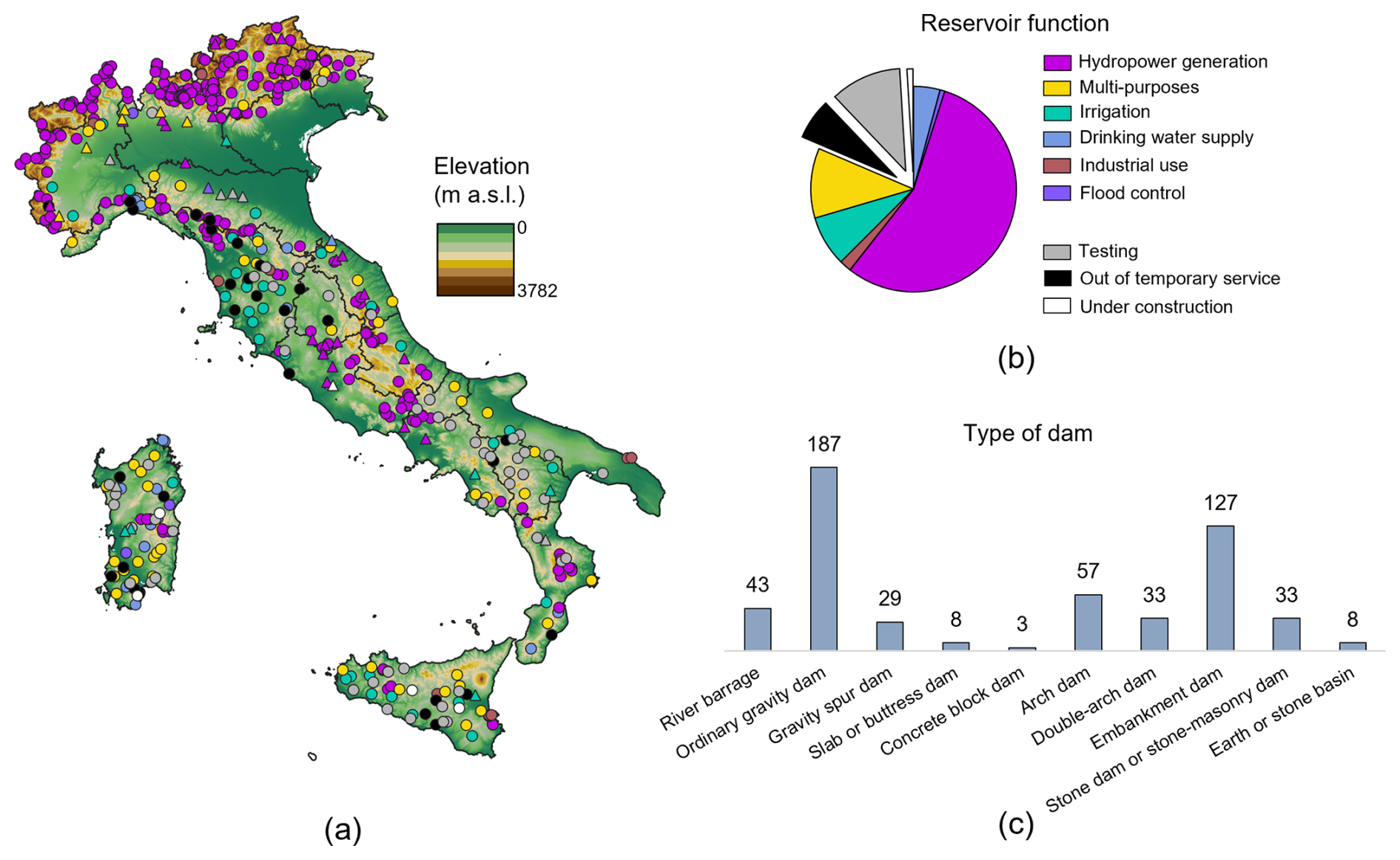
Figure 1 Spatial distribution of the 528 Italian large dams (a), with an overview of their functions (b) and construction types (c). The triangles in panel (a) correspond to river barrages, while all the other dams are identified by circles.

Currently, about 20 % of the reservoirs are temporarily out of service (black colour in Fig. 1a), with some no longer storing water, undergoing functional and technical tests (grey colour in Fig. 1a) or being constructed (white colour in Fig. 1a). Southern Italy has the highest concentration of dams undergoing testing.

Approximately 8 % of the 528 reservoirs supervised by the GDD are classified as river barrages and are marked with triangles in Fig. 1a. According to the technical literature, here the term “river barrage” refers to a structure designed to create a contained backflow within the riverbed. Its primary purpose is to raise the upstream water level to enable water diversion and, more broadly, regulate water levels. Consequently, a river barrage is not typically intended for water storage. Some of these structures are located at large natural lakes, regulating water outflows, ensuring the stability of water levels and supporting specific water management objectives. Some examples include the Miorina barrage (which controls the water outflows from Lake Maggiore), Olginate (which regulates the Adda River and the water level of Lake Como), Salionze (which manages the water level of Lake Garda) and Sarnico (which controls the water release from Lake Iseo).

Table 1 Descriptive features of the dams.

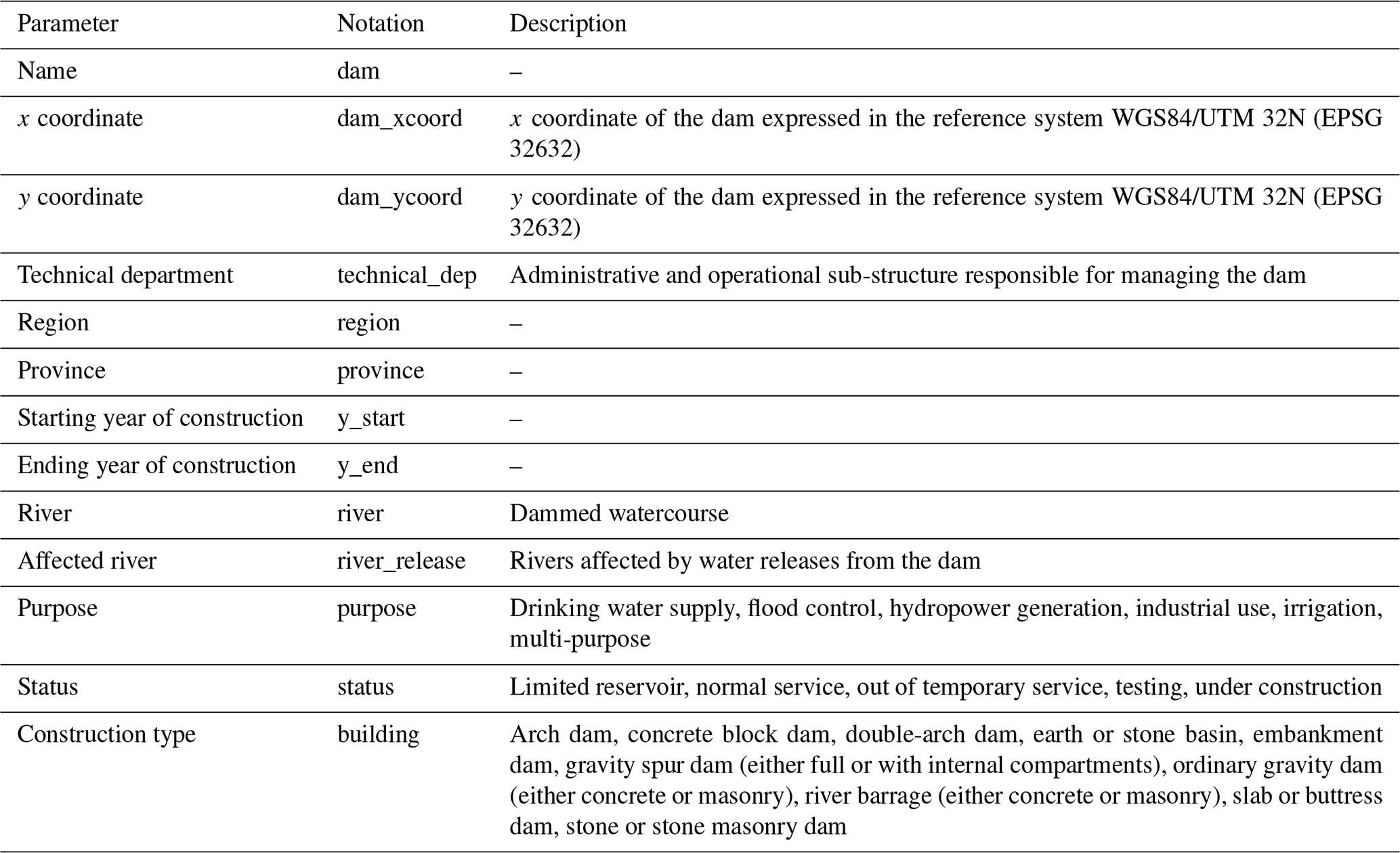
In this paper, all the characteristics discussed above, along with additional information, such as the coordinates of the dam and the years of the start and end of construction, are listed in Table 1 and are available for each dam. The geographical coordinates, sourced from the GDD, have been carefully checked manually using GIS software in order to verify that they actually matched the dam wall at “metre” accuracy.

A significant number of the large dams in Italy date back to the middle of the 20th century, as shown in Fig. 2, which illustrates the total number of dams built in each year from 1870 to 2010 (represented by the points) and the year in which each dam was completed (represented by the lines). The influence of World War II is clearly evident in the break in dam construction (red arrow in Fig. 2), while the highest growth rate occurred between 1950 and 1970. Knowing the temporal distribution of the dams and, in particular, the end year of construction is crucial for conducting accurate flood frequency analyses (e.g. Villarini et al., 2011; López and Francés, 2013) and calibrating and updating hydrological models (e.g. Chaudhari and Pokhrel, 2022).

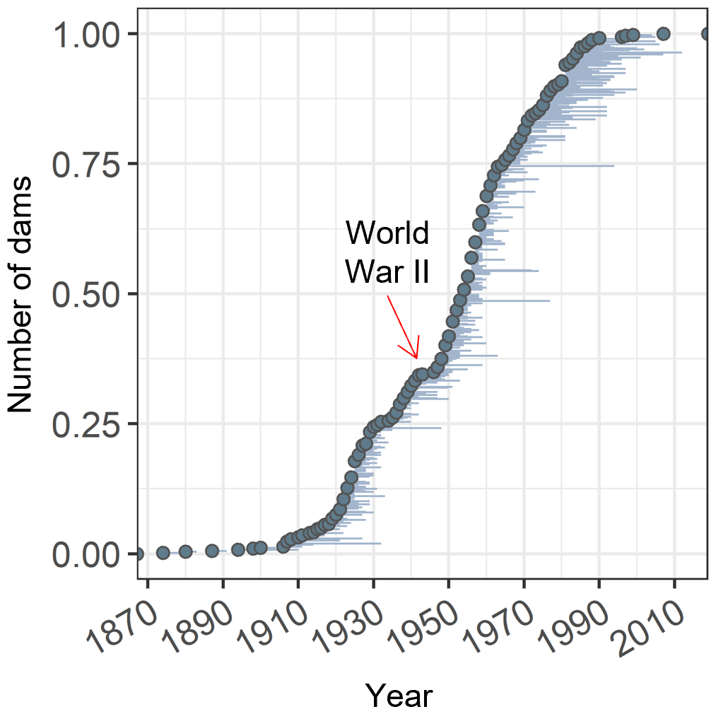
Figure 2 Total number of dams, expressed as a percentage, whose construction started in each year between 1870 and 2010 (points), with the year of completion of each dam's construction (lines). The red arrow highlights a disruption in dam construction during World War II. Dams currently under construction or lacking available start and end construction dates have not been included.

Some of the 528 structures serve as secondary dams, i.e. additional dam structures built within a single lake system. These are shown in Table A1 of Appendix A. In this paper, the term “secondary” refers to a dam that is smaller in size than the main one.

3 Structural features of the dams

Information about the main structural features of the Italian dams has been obtained from the GDD. An overview of these characteristics, together with a summary description, is available in Table 2, while Fig. 3 shows the spatial distribution and variability of storage volumes and lake areas all over Italy. While dam height and storage volume are easily accessible data, what distinguishes this dataset from similar ones is first the inclusion of the lake area. Although this information can be found in the GDW dataset (Lehner et al., 2024), it should be recalled that there are only about 60 % of Italy's large dams represented in that collection. Furthermore, the elevation above sea level corresponding to the reported lake area is not clearly specified. Information on the lake area is crucial when conducting assessments of the dam's ability to mitigate flood peaks, as the reservoir surface area exerts a direct influence on the dam's capacity to manage excess water during periods of high flow. This parameter is directly involved, for instance, in the computation of the Synthetic Flood Attenuation Index (SFA) developed by Miotto et al. (2007). In a more recent study, Cipollini et al. (2022) introduced an index that quantifies the impact of a reservoir in mitigating flood peaks and that relies on the following parameters: (i) the area of the upstream catchment, (ii) the lake area, (iii) the spillway length and (iv) the slope n of the intensity–duration–frequency rainfall curve (see Eq. 2 in Sect. 4.2.4).

Table 2 Structural features of dams.

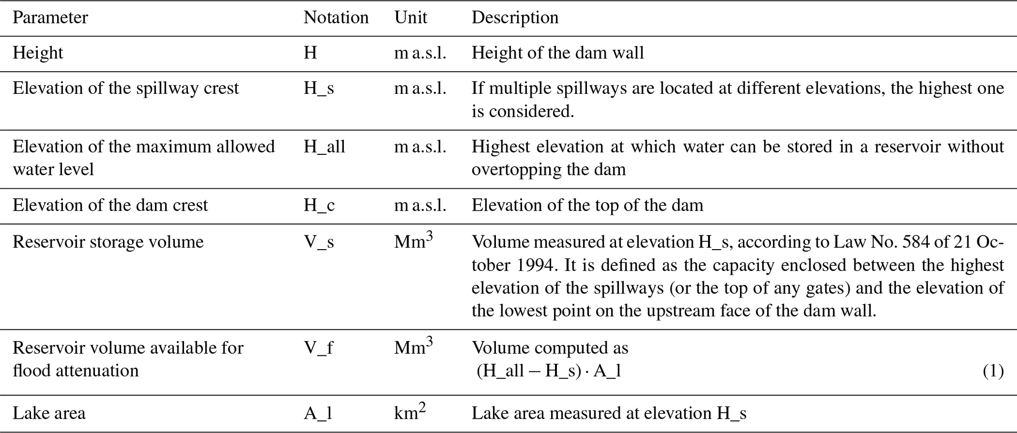
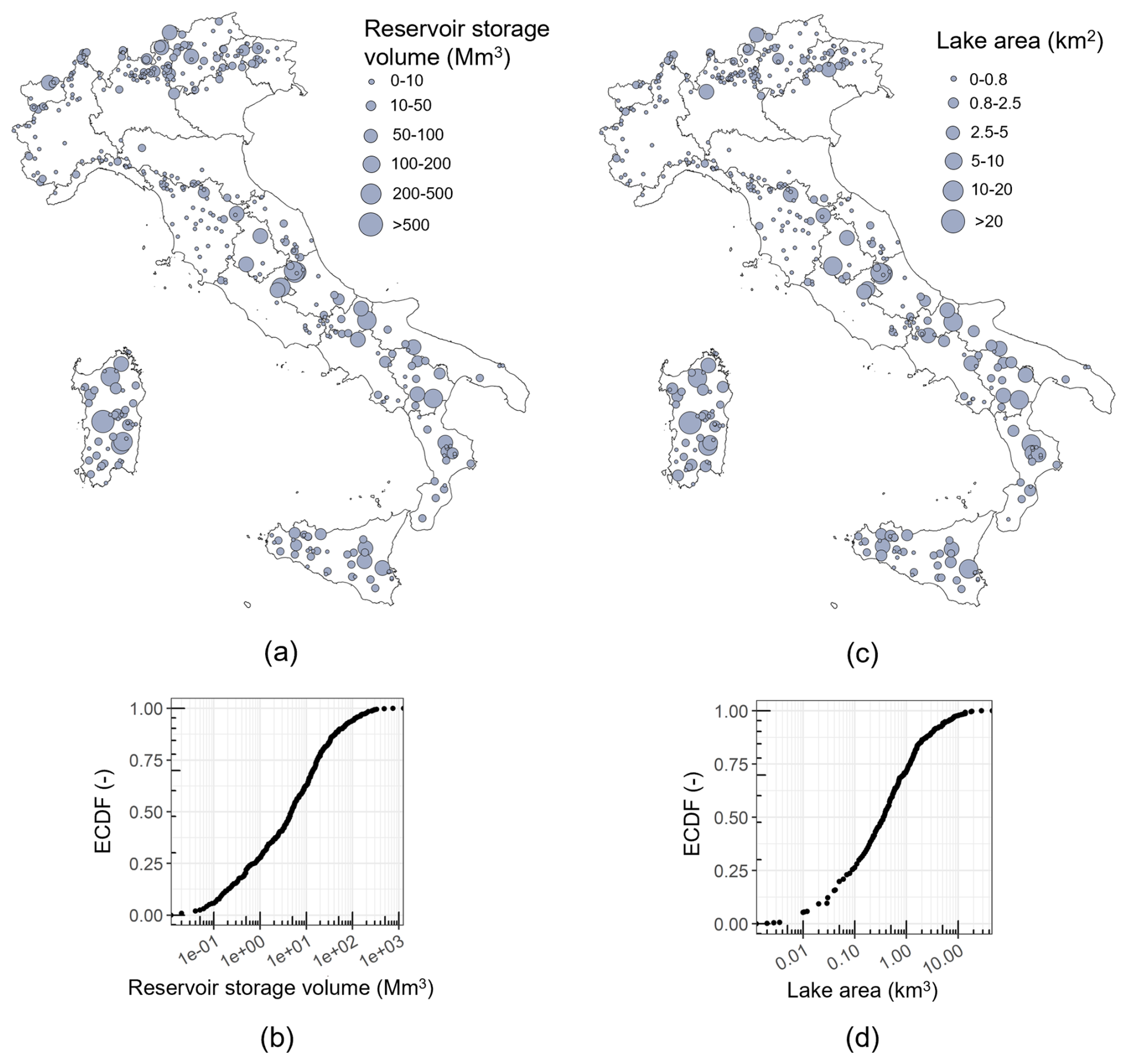
Figure 3 Variability, all over Italy, of storage volumes (V_s) and lake areas (A_l): spatial distributions (a, c) and empirical cumulative distribution functions (ECDFs) (b, d). The ECDF is defined as $\frac{i}{N}$ for $i=\mathrm{1},\mathrm{\dots },N$, where i is the ordered variable for each reservoir. River barrages and temporarily out-of-service dams have not been included.

The elevation corresponding to the maximum allowed water level is another piece of information that one should not overlook. By subtracting the elevation of the spillway crest from this elevation, one obtains a metric that, when multiplied by the lake area, directly provides an estimate of the volume available for flood mitigation (Eq. 1 in Table 2). Furthermore, the wider the gap between these two elevations, the greater the potential for using the reservoir for flood mitigation while retaining the whole volume for hydropower generation or storage of irrigation supplies. Data related to the elevation of the maximum allowed water level are rarely made available in the already released databases.

In order to ensure the accuracy and reliability of the lake area measurements, careful validation has been undertaken. This has involved a systematic comparison of the values retrieved from the GDD with those acquired from a high-resolution DEM, i.e. the TINITALY/01 DEM at 10 m resolution (Tarquini et al., 2007), at the elevation corresponding to the spillway crests. In the case of major differences, the lake area values have been corrected, also by checking the dam design reports. It must be specified that in the case of river barrages the lake area is not provided, as it cannot be identified unequivocally. For dams currently out of temporary service (indicated by the black dots or triangles in Fig. 1a), a null lake area has been assigned.

It must be specified that the structural characteristics of the dams are presented without uncertainty information, as the data were retrieved from officially controlled sources, which minimizes the need for additional uncertainty assessments.

Figure 4 illustrates the relationship between reservoir storage volumes and their surface areas. A linear relationship is found on a log–log graph, and the corresponding power-law fitting equation is provided. The relationship depicted in Fig. 4 has a practical value as it shows that, in cases where the lake area is not known, one can still approximate it using the reservoir storage volume as a good proxy.

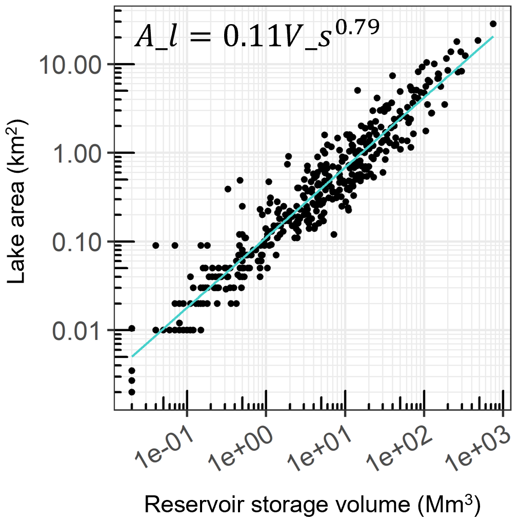
Figure 4 Relationship between reservoir volumes (V_s) and their surface areas (A_l). River barrages, secondary dams and temporarily out-of-service dams have not been included to fit the equation shown in the figure.

4 Morphological and climatic characterization of the upstream catchments

Italy, like many other countries globally, is experiencing shifts in climatic patterns due to climate change (van Vliet et al., 2015; Bombelli et al., 2019). The incumbent increasing frequency and intensity of extreme events (Libertino et al., 2019; Mazzoglio et al., 2022) pose new challenges for dam safety. Historical flood data may no longer represent the full range of potential flood events, and this would entail a re-assessment of spillways' design flood to accommodate changing hydrological conditions, as already stated 10 years ago by Bocchiola and Rosso (2014). Insufficient knowledge of basic hydrological information in areas where dams are located, in view of the need for flood attenuation plans and re-assessment of dam hydraulic safety, was also stressed by the Italian Committee on Large Dams (ITCOLD, 2023). Accurate and up-to-date information about a catchment's hydrological response is crucial then for reconsidering the potential flood scenarios that a dam may face. Furthermore, in 2018 the GDD proceeded to update the directives established in 2000 (directive nos. SDI/7128 and SDI/8111), specifically focusing on the reconstruction of incoming hydrographs (directive no. 3356, retrieved from https://www.dighe.eu/normativa/allegati/2018_Circ_DGDighe_13-02_n_3356.pdf, last access: 10 January 2024). These updated regulations now mandate dam managers and concessionaires to reconstruct the most severe hydrological event of a year, in addition to one or more significant events from the previous 5 years (Santoro et al., 2023). Within this framework, factors such as catchment size, shape, slope and land cover play a significant role in allowing us to calibrate models for the estimation of a flood hydrograph and its peak flow.

The following sections provide a description of the process used to delineate the basin boundaries, along with an overview of the computed attributes for each catchment. The list of attributes, together with the rationale and the methodologies adopted, is the same as that presented in Claps et al. (2024), where 631 gauged watersheds were characterized from a climatic, soil and geomorphological point of view. The choice to provide the same basin attributes comes from the possibility of increasing hydrological knowledge throughout Italy, almost doubling the number of basins where the same level of information is available.

4.1 Catchment boundaries

The boundaries of the upstream catchments were computed by processing the Shuttle Radar Topography Mission (STRM) DEM at 30 m spatial resolution (Farr et al., 2007). The selection of the SRTM DEM, despite its coarser resolution compared to TINITALY/01 (Tarquini et al., 2007) or TINITALY/1.1 (Tarquini et al., 2023), is based on considerations about how the TINITALY DEMs are compiled. These latter ones are composite DEMs created by merging different regional or local DEMs, which means that they do not maintain a consistent level of accuracy nationwide. To address this issue, we opted to use the SRTM DEM.

The processing of the DEM has been carried out using the r.basin GRASS GIS add-on (Di Leo and Di Stefano, 2013), following the procedure described in Fig. 1 in Claps et al. (2024). The process of establishing basin boundaries includes calculating drainage directions, determining flow accumulation, and finally extracting the stream network with a specified threshold value for channel initiation. Here a minimum area of 0.1 km² was adopted to extract basins larger than 1 km². Otherwise, a threshold of 0.02 km² was used.

As expected, the automatic delineation procedure did not exhibit major problems, since the basins analysed are typically located in mountainous areas, where elevation differences are quite pronounced. In a couple of cases, where the topography posed difficulties for automated delineation, basin masks were created manually, i.e. forcing the DEM to correct the total contributing area (TCA) map built by the r.basin procedure, a technique commonly referred to as stream burning (Lindsay, 2016). When needed, this operation was conducted by comparing the unconstrained river network generated by r.basin with the reference one provided by ISPRA (available at http://www.sinanet.isprambiente.it/it/sia-ispra/download-mais/reticolo-idrografico/view, last access: 31 March 2025). Only two watersheds required stream burning: that upstream of the Panaro dam in Emilia-Romagna and that upstream of the Lago Pusiano dam in Lombardy. Both of these basins mainly include flat areas characterized by the presence of several artificial diversions. The Lago Pusiano dam area has also undergone substantial urbanization. On the other hand, five reservoirs, i.e. the Gerosa dam (Marche), the Presenzano dam (Campania), the Vasca di Edolo dam (Lombardy), the Vasca Ogliastro dam (Sicily) and the Vasca Sant'Anna dam (Calabria), do not possess a directly associated catchment area. This is either because they have very little to no upstream contributing area, as in the case of the Gerosa dam, or because they serve as off-stream reservoirs, storing water outside the natural course of a river. Therefore, information regarding the upstream catchments for these dams is unavailable, which reduces the total number of basins collected in this database to 523.

Since the geographical coordinates of the dam do not necessarily coincide with those of the basin outlet, i.e. those used operationally when defining the catchment boundaries, a pair of coordinates other than those listed in Table 1 is provided. They are referred to as “operational coordinates” and are named basin_xcoord and basin_ycoord in the dataset.

The reliability of watersheds automatically extracted from a DEM is inherently influenced by several factors. These include the resolution and accuracy of the DEM itself, the precision and robustness of the extraction algorithm and the handling of specific landscape features such as flat areas and depressions. Errors in the DEM, such as noise or inaccuracies in elevation data, can propagate through the watershed delineation process, leading to potential misrepresentations of watershed boundaries and the associated topographic features. Consequently, it is crucial to assess and validate these automatically delineated watersheds against ground truth data or higher-quality references.

As mentioned above, DEM conditioning procedures were only necessary in a very few cases in our study. To ensure the accuracy of the basin contours determined using the above-mentioned procedure, some verification steps were taken. In the first instance, Google Earth was employed. The delineated watershed boundaries were cross-referenced with visual representation of the surrounding terrain offered by Google Earth, ensuring that they coincided with the natural ridges and topographical features of the area. Then the basin area values were compared with those reported in Policicchio (2020), as will be discussed in Sect. 4.2.1.

4.2 Catchment attributes

Derivation of all the catchment boundaries as described in the above section allowed us to calculate several catchment-averaged attributes. The attributes computed are the same as those provided in Claps et al. (2024) and can be grouped into four main categories as (i) geomorphological attributes; (ii) soil attributes, land cover, and NDVI (Normalized Difference Vegetation Index); (iii) climatological attributes; and (iv) attributes related to extreme rainfall. Hence, while not explicitly reported in the main body of the paper, tables listing all the descriptors provided can be found in Appendix B.

It is important to recognize that all the attributes presented in this section are associated with some degree of uncertainty. As mentioned earlier, potential inaccuracies in geomorphological descriptors should be considered in relation to the processing of the DEM. On the other hand, uncertainties in soil, land cover and climatological attributes, which are computed from existing raster datasets, may result from interpolation or spatial resampling procedures. While we will explore the uncertainties related to geomorphological descriptors in more detail below, readers can refer to Claps et al. (2024) for an in-depth discussion of the uncertainties associated with the other descriptor categories.

4.2.1 Geomorphological attributes

This category of attributes was computed by using additional algorithms to r.basin, i.e. the r.stat, r.slope.aspect, r.stream.stats (Jasiewicz, 2021) and r.accumulate (Cho, 2020) functions, as described in Claps et al. (2024).

In Fig. 5a and b, each dot represents a dam, and its colour indicates the mean elevation (a) and mean slope (b) of the upstream basin. The point size corresponds to the basin area, normalized with respect to the largest basin within the dataset, i.e. the one upstream of the Isola Serafini river barrage (in between Emilia-Romagna and Lombardy). From the overall picture of the 523 watersheds, one recognizes that the set of basins is composed of mainly small, mountainous basins, as almost 75 % of them have a normalized area of less than 0.2 and approximately 50 % of them have an average slope of over 20 %. Almost 40 dams have an area of less than 1 km². It must be specified that the analysis focused solely on the watersheds directly connected to the reservoirs, without considering any indirectly connected basins. In other words, areas that are part of the reservoir management system but do not lie within the natural contributing basin upstream of the dam were not considered. In Fig. 5c, the variability of empirical hypsometric curves for the 523 basins is depicted, showing rather different morphometric characteristics across the dataset.

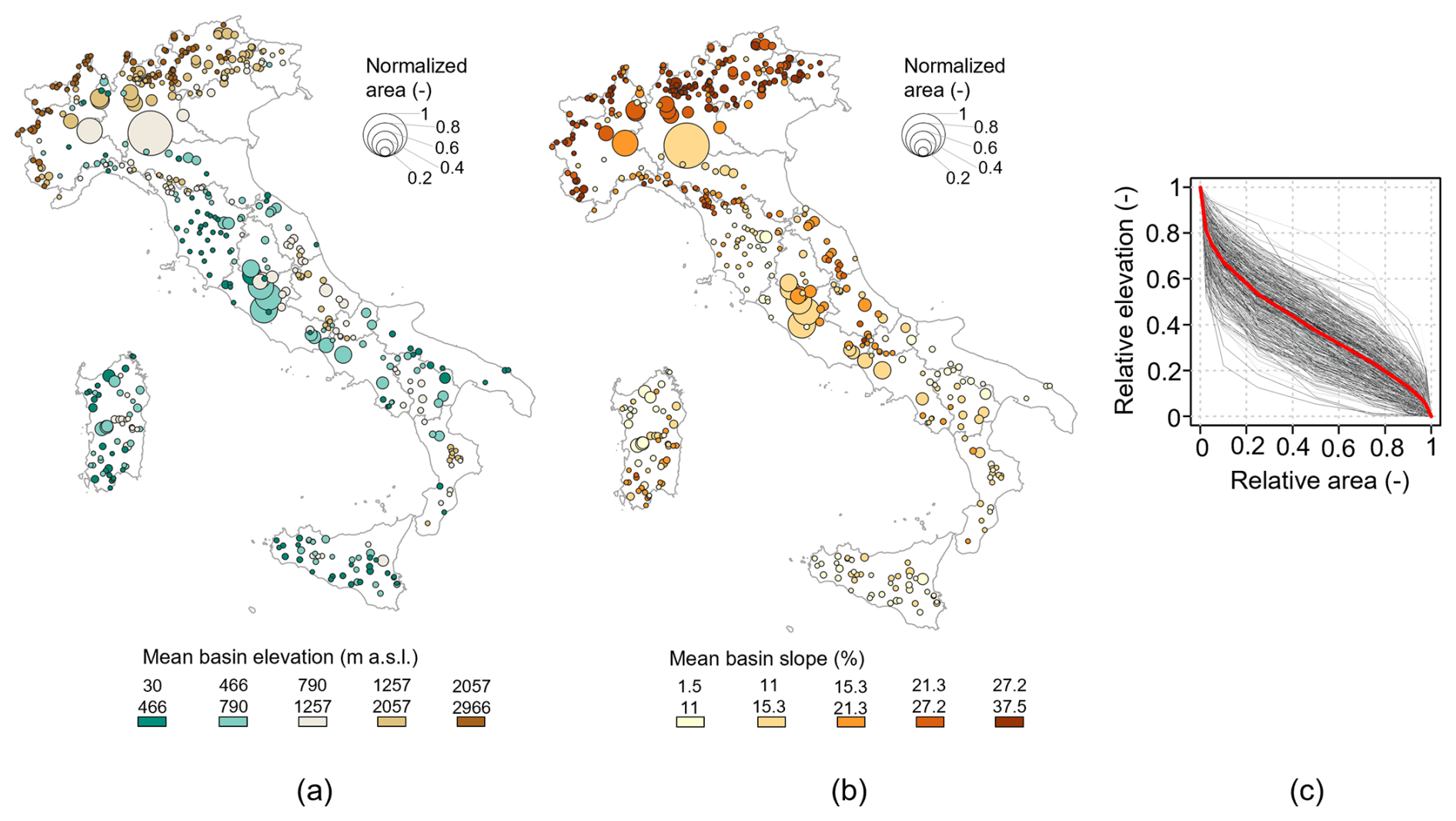
Figure 5 Mean elevation (a) and mean slope (b) of the 523 basins. The point size represents the basin area normalized to the maximum value within the dataset. Empirical hypsometric curves of each basin (in grey) and average hypsometric curve (in red) (c).

The only available benchmark for controlling basin areas is a report provided by ISPRA (Policicchio, 2020). Titled “Water Resources in the Geological Context of the Italian Territory: Availability, Large Dams, Geological Risks, Opportunities”, this report aims to gather information on water resources, particularly their use in the context of artificial barriers like dams. It also explores the relationship between water resources and various natural hazards, including seismic, tectonic, geomorphological and hydraulic risks. We have compared the basin area values published in the above report with those determined using the r.basin algorithm, and the resulting scatterplot is presented in Fig. 6a. Notably, the basin areas reported by Policicchio (2020) tend to be higher than those directly computed here, particularly for basins smaller than 100 km². This discrepancy is likely due to inaccuracies in outlet coordinate placement or the inclusion of indirectly connected basins in the computation of the upstream area. It is important to consider that employing a DEM with a coarser resolution (not specified in Policicchio, 2020) may have played a role in the observed discrepancies, exerting a more significant impact on smaller areas. Given that manual adjustments (stream burning) were necessary for only 2 basins out of 523 and that the areas were derived directly from DEM processing, it can be concluded that the calculated areas are reasonably accurate. As an additional quality control, the consistency between the length of each basin's main channel and that of its longest drainage path has been assessed. As detailed in Claps et al. (2024), this procedure aims to identify potential weaknesses in the delineation procedure. Ad hoc checks highlighted occasional issues in the GIS procedure for computing the main channel length and the longest drainage path length. Two problems were observed: (i) the main channel shapefiles contained multiple features that required merging, and (ii) multiple longest drainage paths were identified for the same catchment, each differing by no more than 100 m. In this latter case, one longest drainage path was chosen manually, and other instances were removed. After these checks, a linear relationship between the length of the main channel and the basin area was found on a log–log graph, as shown in Fig. 6b and discussed in Claps et al. (2024).

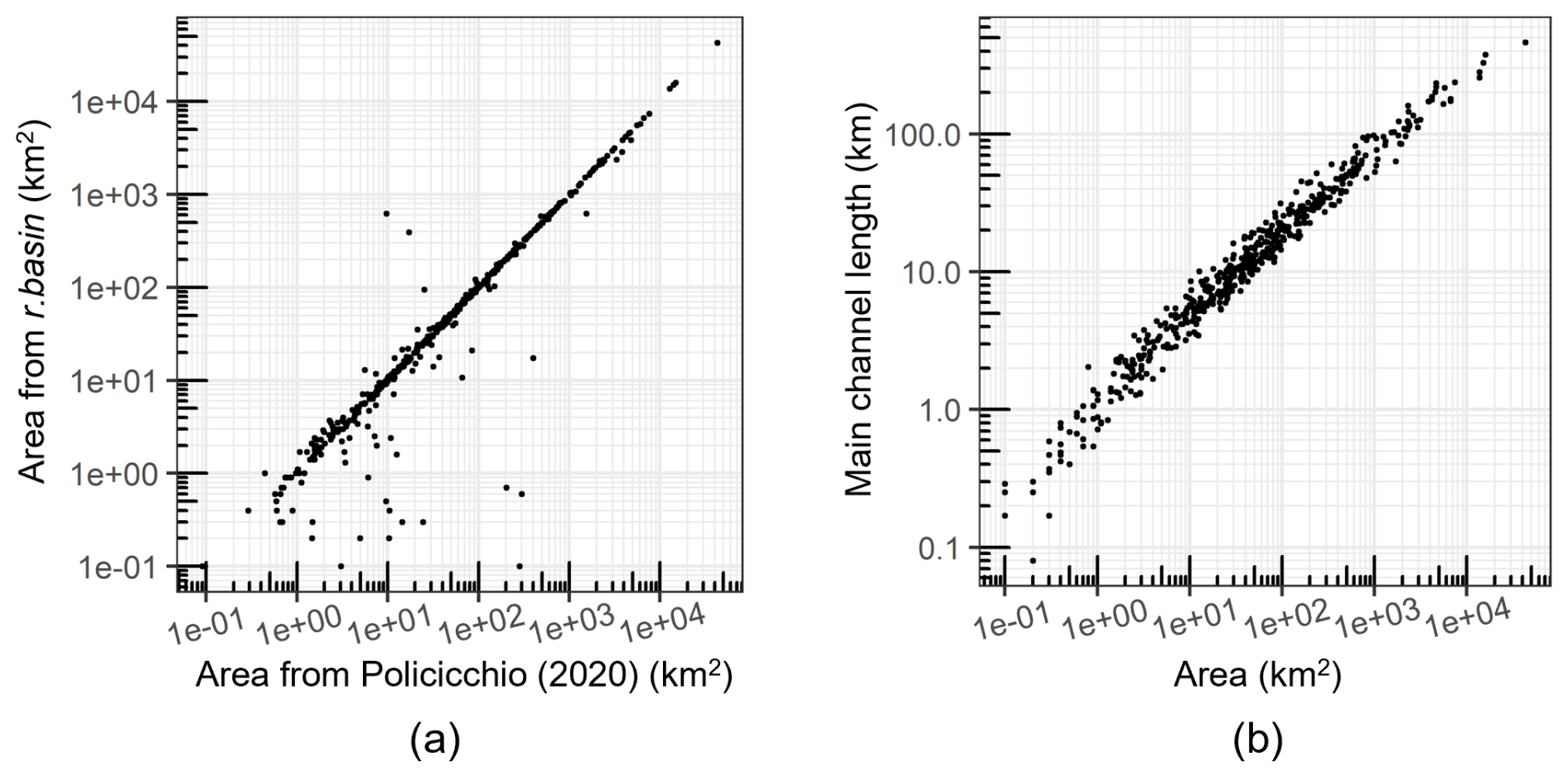
Figure 6 Quality controls on geomorphological parameters. Comparison of area values obtained from the delimitation procedure and those reported in Policicchio (2020) (a). Relationship between the main channel lengths and the basin areas (b).

4.2.2 Soil, land cover and NDVI attributes

For each catchment, spatially averaged information on soil, land cover and the NDVI was computed. Similarly to the other categories of attributes, the list of soil, land cover and NDVI attributes provided is analogous to the one reported in Claps et al. (2024), and the reader will find it in Appendix B (Tables B2 and B3). The dataset encompasses soil descriptors that offer insights into area-averaged soil permeability conditions, like the curve number (Soil Conservation Service, 1972) and the saturated hydraulic conductivity.

The curve number is an empirical parameter that assesses the proportion of total rainfall converted into net rainfall during a flood event. Three different values for the curve number (CN1, CN2 and CN3) are available, each corresponding to specific antecedent wetness conditions of the soil (i.e. dry, average or wet conditions, respectively). For each of these three curve numbers, the spatial mean value and the spatial coefficient of variation were computed. Consistent with Claps et al. (2024), the data sources used are the curve number national-scale raster maps at 250 m resolution computed by Carriero (2004).

The mean saturated hydraulic conductivity was computed using the pedotransfer function proposed by Saxton et al. (1986). For its application, which requires sand and clay contents, we employed soil texture fraction values extracted from the SoilGrids maps (Hengl et al., 2017; available at https://soilgrids.org/, last access: 31 March 2025). These maps delineate soil property parameters at 250 m spatial resolution all over the world across seven standard depths from 0 to 200 cm. These were computed using over 230 000 soil profile observations from the WoSIS (World Soil Information Service) database (Batjes, 2009). To align the information produced with the hydrological context of this study, we averaged the soil texture information over the initial 30 cm of the soil depth, which is consistent with Claps et al. (2024). This depth range is often regarded as representative of the topsoil layer, which is essential for supporting vegetation and regulating both water retention and drainage processes.

Land cover characteristics were derived from the 100 m spatial resolution third level of CORINE Land Cover 2018 (available at https://land.copernicus.eu/, last access: 31 March 2025). This involved the redistribution of 44 land cover classes into five distinct land indices, i.e. clc1 (associated with urbanized areas), clc2 (related to arboreal vegetation), clc3 (corresponding to herbaceous vegetation and crops), clc4 (associated with non-vegetated and industrial areas) and cl5 (related to humid areas). For each catchment, we provided the percentage covered by each of these five classes.

Data related to the stability of vegetation over time within the basin, in terms of growth, health and coverage, were assessed further by means of the NDVI. The NDVI metric provides measures of vegetation density and health, offering information about land use changes and potential impacts on hydrological processes, specifically the way water is absorbed and released through plant transpiration. Multi-temporal indicators of the NDVI were computed from the Copernicus Land Monitoring Service (available at https://land.copernicus.eu/, last access: 31 March 2025) Long Term Statistics (LTS) NDVI V3.0.1 with a spatial resolution of 1 km. This dataset was used to evaluate NDVI mean observations spanning the 1999–2019 period for each of the 36 10-daily periods, resulting in 36 raster maps. These maps facilitated the computation of the mean annual NDVI value, the (temporal) coefficient of variation of the NDVI and the spatio-temporal mean NDVI regime. The latter was characterized synthetically using a Fourier series representation that allows the description of the shape of the regime with only four parameters. This representation provides a more concise overview than the 36 individual 10 d average values. More details about the computation of the four coefficients of the Fourier series are available in Claps et al. (2024).

4.2.3 Climatological attributes

National-scale datasets with a resolution of 1 km were employed to assess various climatological attributes that allow us to describe the precipitation and temperature climatology of these catchments.

Mean monthly precipitation data were extracted from the BIGBANG 4.0 dataset (Bilancio Idrologico GIS Based a scala Nazionale su Griglia regolare; Braca et al., 2021). Spanning the period from 1951 to 2019, this dataset applies spatial interpolation at 1 km resolution to rain gauge measurements. It also incorporates already available spatial interpolations from ArCIS (Archivio Climatologico per l'Italia Centro Settentrionale; Pavan et al., 2019) in limited areas and for specific years. The mean monthly temperature information is similarly derived from this dataset.

Catchment boundaries were used to clip the aforementioned precipitation and temperature maps, enabling the derivation of spatial averages for the 14 climatological attributes.

Similarly to what was done for the NDVI averages, monthly precipitation depths and monthly temperature data were processed to calculate the mean coefficients of the Fourier series, providing an approximation of the precipitation and temperature regimes (four coefficients for rainfall and four for temperature, as described in Claps et al., 2024). The original monthly raster maps were also used for the evaluation of the temporal coefficient of variation of rainfall regimes and the time lag between the maximum and minimum of the mean monthly rainfall.

The same dataset was employed to determine the mean annual precipitation (MAP) and mean annual temperature (MAT) basin-averaged values, together with their spatial coefficients of variation.

4.2.4 Extreme rainfall attributes

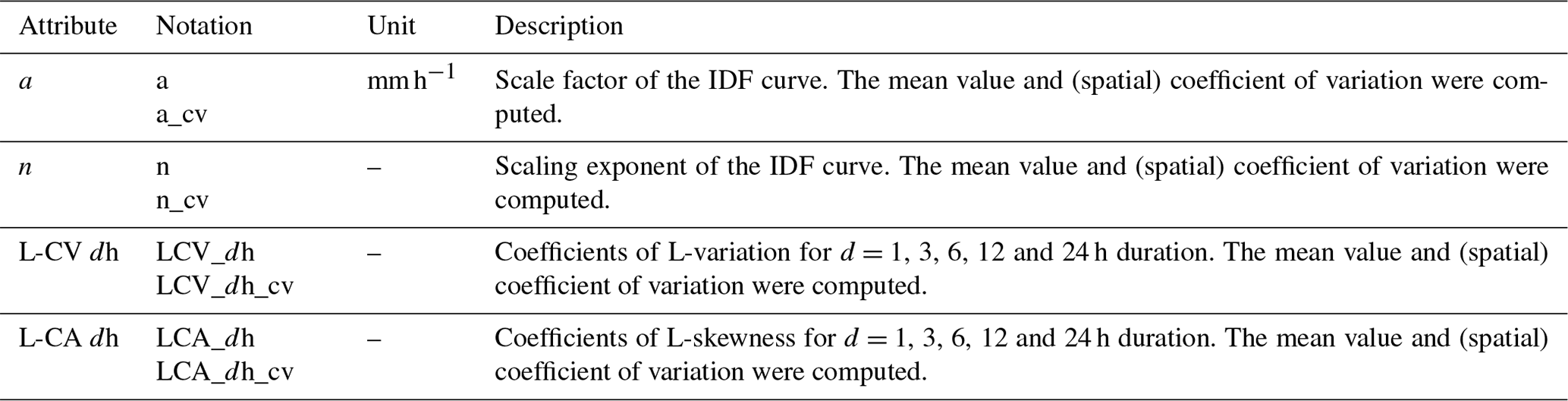
According to the index value approach (Darlymple, 1960), based on the “simple scaling” hypothesis (Burlando and Rosso, 1996), the quantile of the annual maximum rainfall depth for the duration d and the return period T can be expressed by means of intensity–duration–frequency (IDF) curves, defined as

$$\begin{array}{}\text{(2)}& h\left(d,T\right)=K_T\cdot a\cdot d^n,\end{array}$$

where a and n are the scale factor and the scaling exponent, respectively, and K_T is the non-dimensional inverse frequency factor, also called the growth factor. Catchment-averaged values of a, n and K_T have been derived in all the considered basins by interpolating values previously determined at the individual rain gauge level. A complete rain gauge network is available in the Improved Italian – Rainfall Extreme Dataset (I²-RED), a collection of short-duration (1, 3, 6, 12 and 24 h) annual maximum rainfall depths measured by more than 5000 rain gauges from 1916 up to the present (Mazzoglio et al., 2020). The at-site a and n rainfall parameters are obtained by means of linear regression of the logarithm of the average rainfall maxima h(d), computed from at-site measurements over the 1–24 h durations with the logarithm of the duration d. The growth factor K_T can be estimated using the sample L-moments of the time series after having defined a specific probability distribution. Time series of at least 10 years of data have been used to estimate a and n, while 20 and 30 years have been set as minimum lengths for the computation of the coefficients of L-variation (L-CV) and L-skewness (L-CA), which have been computed using Eqs. (6) and (7) of Laio et al. (2011), respectively.

At-site rainfall statistics were then spatially interpolated at 250 m resolution with the autokrige R function (Hiemstra and Skoien, 2023). We calculated catchment-averaged values for a and n as well as the basin mean L-CV and L-CA coefficients for the durations of 1, 3, 6, 12 and 24 h to compute a catchment-averaged K_T.

Again, the list of rainfall attributes provided is analogous to that reported in Claps et al. (2024), and the reader will find it in Table B5 in Appendix B. Figure 7a and b show the outcome of the spatial averaging process applied to parameters a and n, respectively, at the catchment level. It is interesting to note an inverse dependence between a and n: regions with high n values, indicating a slow decrease in rainfall intensity with the duration, tend to exhibit low a values, which represent the average maximum rainfall over a 1 h duration. This pattern is particularly evident in Alpine regions and, as shown by Evangelista et al. (2023), contributes in part to justifying the significant flood attenuation capacity of Alpine dams.

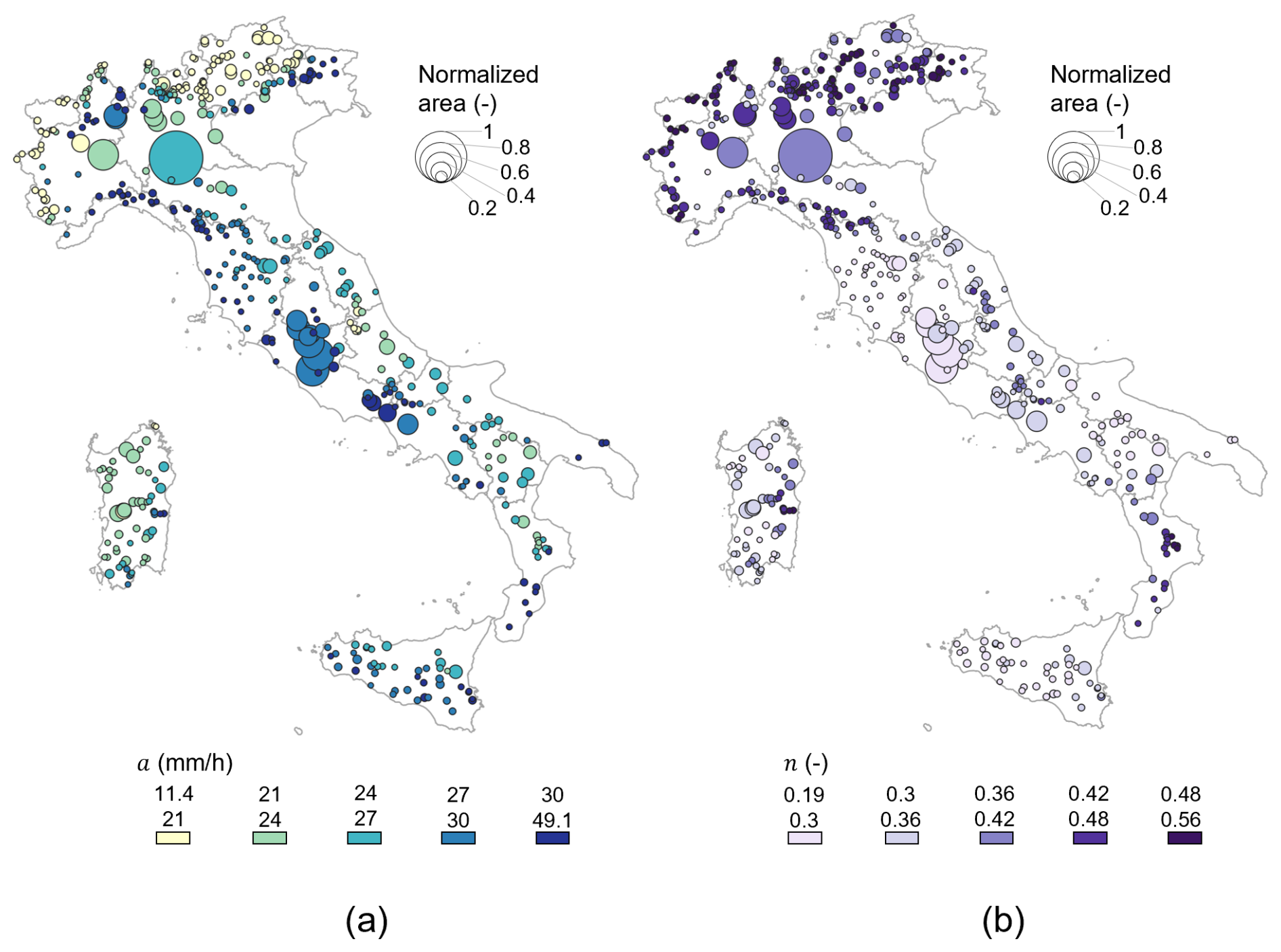
Figure 7 Spatial representation of the mean basin parameters a (a) and n (b) of the IDF curves. The point size represents the basin area normalized to the maximum value within the dataset.

5 Interaction between the infrastructure and the upstream basin

As mentioned in the Introduction section, dams can play a significant role in mitigating the impacts of flood events, providing some level of protection to downstream areas. Well-known examples in Italy are those of the Maccheronis dam (Sardinia), which, while not specifically designed for flood attenuation purposes, significantly reduced the natural flood peak during the Cleopatra storm in 2013 (Brath, 2019). Similarly, during the Vaia storm that hit north-eastern Italy in 2018, the Ravedis (Friuli Venezia Giulia), Corlo (Veneto) and Pieve di Cadore (Veneto) dams played essential roles in managing floodwaters (Baruffi et al., 2019). The Chiotas and Piastra (Piedmont) reservoirs also provided assistance during a particularly intense weather event that affected the Piedmont region in October 2020 (Basano et al., 2021). These examples underscore the importance of considering unsupervised flood attenuation, i.e. based on the inherent characteristics of the landscape and reservoir (Evangelista et al., 2023), in comprehensive flood risk management strategies.

Some basic metrics are used in the literature to roughly quantify the infrastructure's effectiveness in mitigating flood peaks. Among these metrics, one useful indicator is the relationship between the lake and the upstream basin areas (e.g. Scarrott et al., 1999; Evangelista et al., 2022), which is depicted in Fig. 8a for Italian dams. All other geometric features being constant, dams with small reservoir areas and large upstream watersheds perform less effectively in flood mitigation than dams with larger reservoir areas and smaller upstream watersheds. Different values for this ratio can be viewed as a threshold below which the reservoir system is deemed to have minimal or no unsupervised attenuation effects. When adopting a ratio of $\mathrm{1}/\mathrm{150}$, as done in Evangelista et al. (2023), one can notice from Fig. 8a that approximately 50 % of the Italian dams (grey points) have negligible efficiency in flood mitigation.

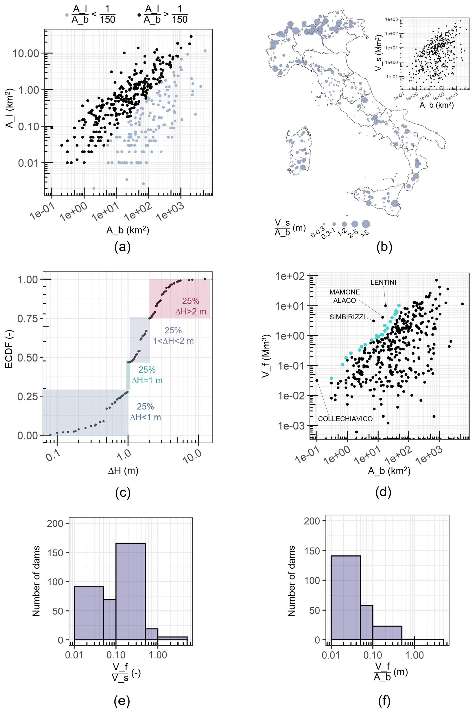
Figure 8 Relationship between the lake area (A_l) and the area of the basin upstream of the dam (A_b) (a). Grey and black dots indicate dams with ratios of lake to upstream basin areas lower or higher than $\mathrm{1}/\mathrm{150}$. Spatial distribution of the ratio between the reservoir storage volume (V_s) and the area of the upstream catchment (A_b) (b). The scatterplot in the right corner shows the relationship between the two variables. ECDF of the difference between the elevation of the maximum allowed water level and that of the spillway crest (ΔH) (c). Relationship between the volume available for flood control (V_f) and the area of the catchment upstream of the dam (A_b) (d). The blue points represent an upper threshold for the growth rate of the available volume with the basin area. Histograms of the ratios of the volume available for flood control (V_f) to the reservoir storage volume (V_s) (e) and to the upstream basin area (A_b) (f).

Another qualitative index for describing the impact of dams on floods is the ratio of the reservoir storage volume to the upstream basin area (e.g. Graf, 2006); dams with higher ratios have greater potential for flood control, as pointed out by Stecher and Herrnegger (2022). Figure 8b illustrates how these ratios are distributed throughout Italy, with particularly high values concentrated across the Alps, while the upper-right scatterplot shows the relationship between the two variables.

In this paper, however, the actual values of flood accommodation capacities are provided for each Italian dam. Users can then easily and accurately assess downstream reservoir impacts without relying on the use of proxies or qualitative indicators. According to Eq. (1), the volume of water that can be stored within the reservoir for flood control purposes depends not only on its surface area, but also on a key second factor, i.e. the difference between the elevation of the maximum allowed water level and that of the spillway crest, hereinafter referred to as ΔH. The empirical distribution of ΔH values for Italian large dams is shown in Fig. 8c. One can see that 75 % of the dams have a ΔH value of less than 2 m, while 25 % of them have a ΔH value equal to 1 m. As mentioned in Sect. 3, the higher the ΔH value, the greater the reservoir's capacity to effectively manage floods while maximizing its utility for hydropower generation or water storage.

In Fig. 8d, the relationship between the volume allocated for flood control and the upstream catchment area is illustrated. The figure shows that the larger the basin drained by the dam, the greater the volume available for attenuating flood peaks. This pattern results from the positive correlation between the lake and basin areas (with a Spearman correlation coefficient of 0.5). The rate of increase in the available volume with the basin area appears to have an upper limit, which is represented by the points marked in light blue in Fig. 8d. This suggests that a threshold exists above which further allocation of volume for flood control would only be possible when reducing the water level under the elevation of the spillway crest and then compromising the primary functions of hydropower generation or storage of irrigation supplies. This threshold is exceeded by only four dams (as highlighted in Fig. 8d), i.e. the Lentini (Sicily), Mamone Alaco (Calabria), Collechiavico (Lazio) and Simbirizzi (Sardinia) dams: they are located in mostly flat areas and are characterized by comparably sized lakes and upstream watersheds, making them singular cases where the usual trade-offs between flood control and other functions are overcome.

A dam's capacity for flood control can be standardized in relation to either the reservoir size or the upstream basin area, making the information more useful than its absolute value alone. Figure 8e and f depict histograms of the ratio of the volume available for flood control to both the reservoir storage volume (Fig. 8e) and the watershed area (Fig. 8f). In the former case, a common range of values typically falls between 0.1 and 0.5, while in the latter case values between 0.01 and 0.05 can typically be observed.

6 Data availability

The dataset detailed in this paper is available at https://doi.org/10.5281/zenodo.14698223 (Evangelista et al., 2024b). It contains all the catchment boundaries and related catchment attributes described before. To access the latest version of the database in case of future updates, readers can go to https://doi.org/10.5281/zenodo.12818297 (Evangelista et al., 2024a) for download.

7 Conclusions

In this work we provide an extensive collection of structural and catchment-related features for the full ensemble of Italian large dams, which represents, to date, the most comprehensive dataset of dams in Italy. The information presented here offers a useful resource for researchers, policymakers and stakeholders involved in water resource management and infrastructure planning.

The structural descriptors encompass information about each dam (year of commissioning, height, type, etc.) and characteristics relating to the associated reservoir (reservoir volume and area, purpose, etc.). Unlike other similar global or national datasets, our work stands out by including information on the lake area and the elevation of the maximum allowed water level. This addition has significant importance, particularly in estimating a dam's capacity to attenuate flood peaks.

Basin characteristics (including geomorphological, soil, land cover and climatic attributes) and basin contours are determined using standardized and uniform procedures, ensuring consistency throughout the country. Taking into account the availability of the “twin” dataset from Claps et al. (2024), a high level of detail is therefore provided on about 1000 watersheds all over Italy, including both dammed and gauged watersheds. Given the challenges posed by climate change and water resource issues, a comprehensive analysis of our current infrastructure will become progressively crucial. In this sense, this work can help to improve our ability to manage the complex interplay between dams and their hosting environments.

Appendix A

Table A1 List of secondary dams.

Appendix B

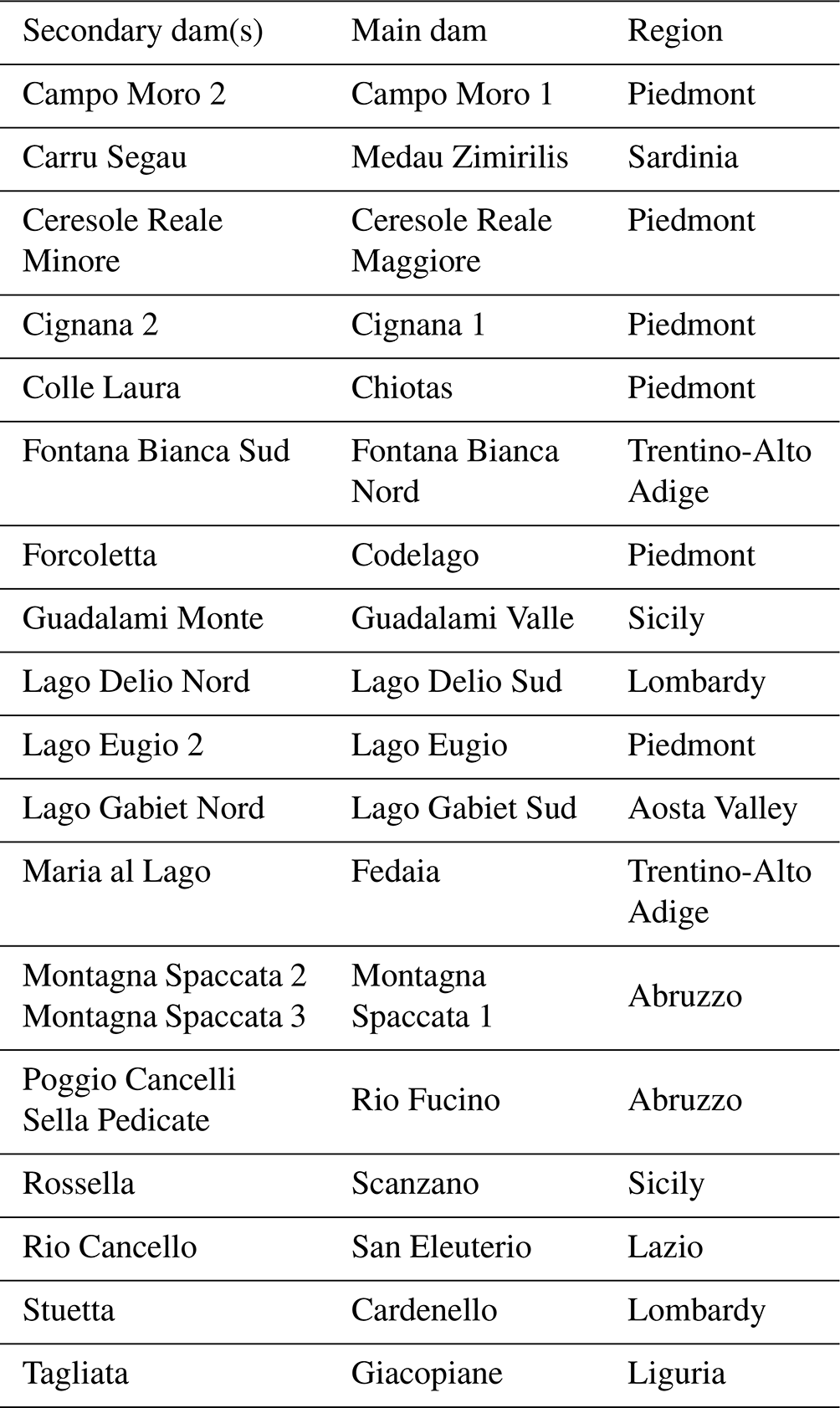
Table B1 List of geomorphological attributes, with a brief description and an indication of the algorithm or add-on used for their computation. All the attributes are computed by processing the SRTM DEM at 30 m resolution with the r.basin add-on, which takes advantage of the other GRASS GIS algorithms mentioned at the beginning of Sect. 3.3 of Claps et al. (2024). Source: Claps et al. (2024).

Table B2 List of soil attributes. Source: Claps et al. (2024).

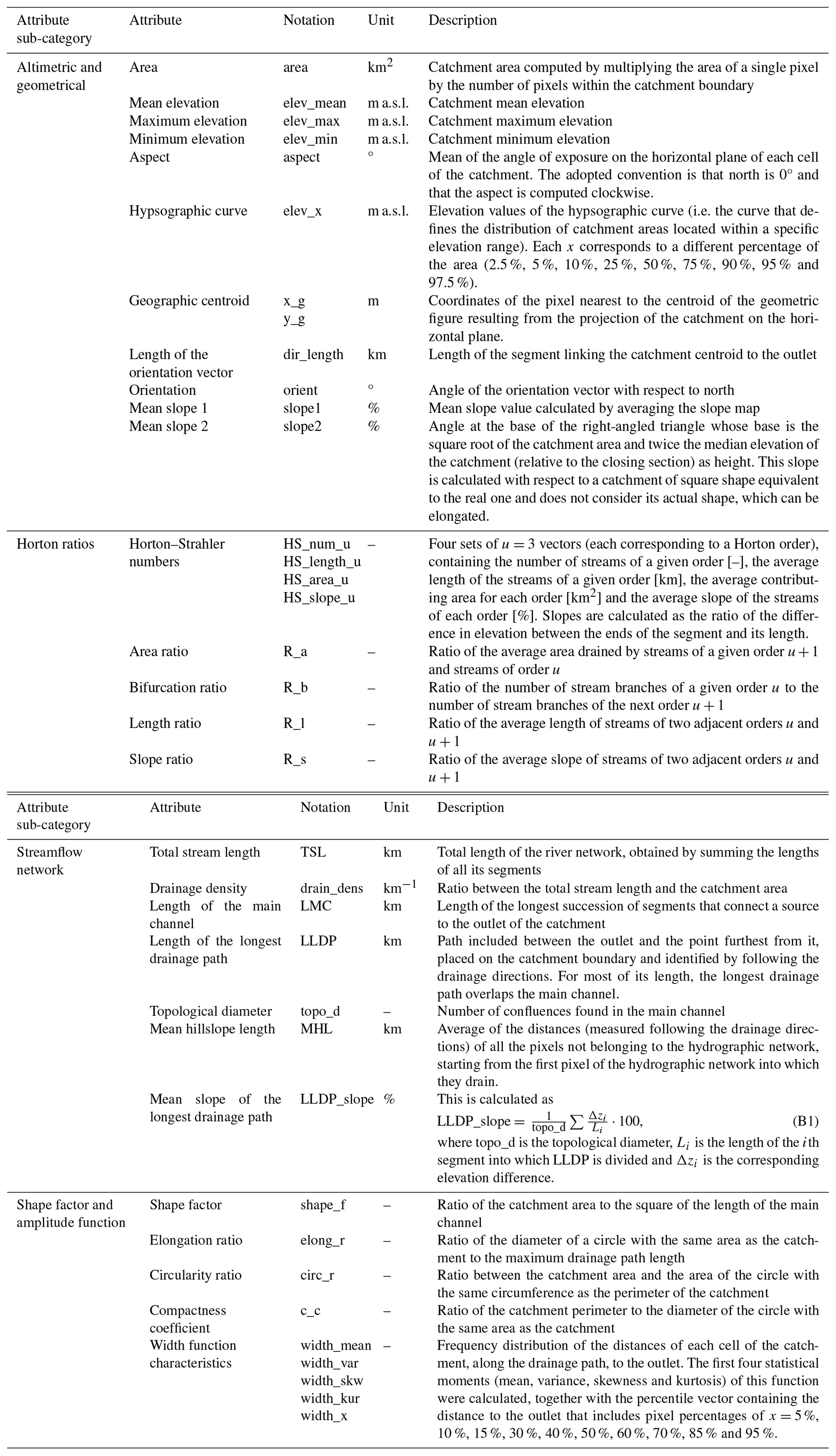
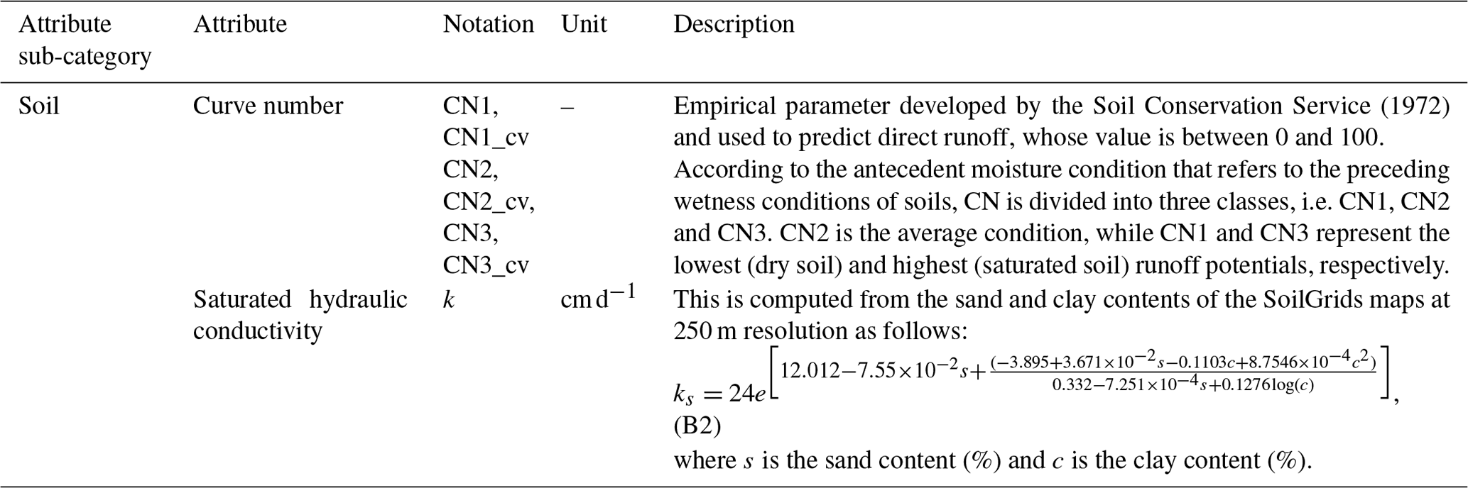
Table B3 List of land cover and NDVI attributes. Source: Claps et al. (2024).

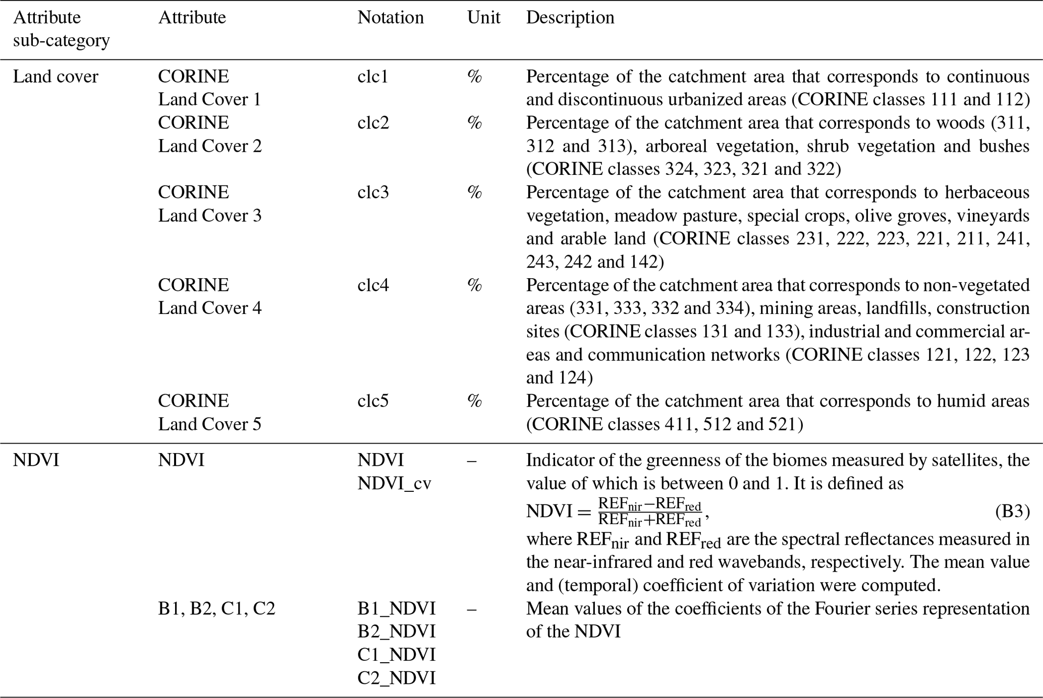
Table B4 List of climatological attributes. Source: Claps et al. (2024).

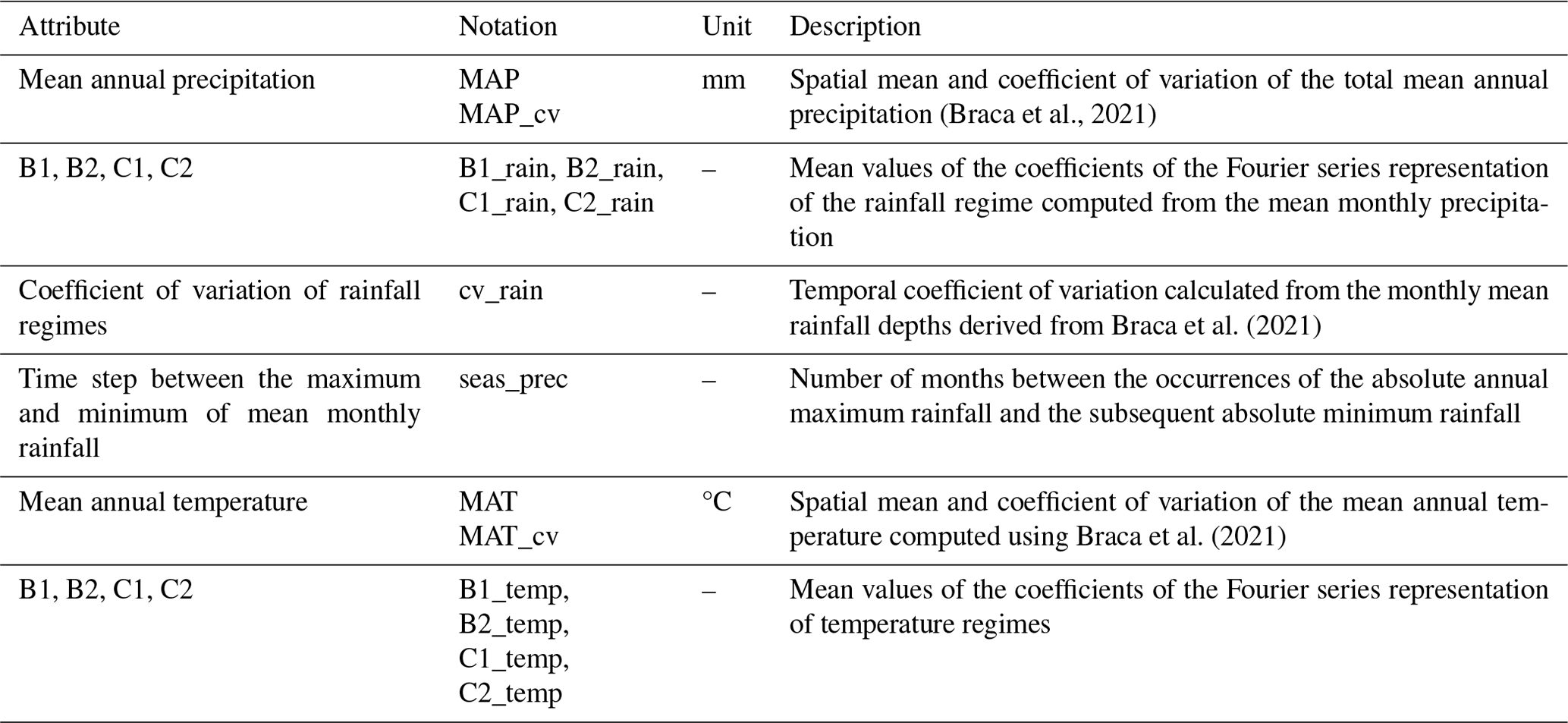
Table B5 List of rainfall attributes. Source: Claps et al. (2024).