EEAR-Clim: a high-density observational dataset of daily precipitation and air temperature for the Extended European Alpine Region

The Extended European Alpine Region (EEAR) exhibits a well-established and very high density network of in situ weather stations, hardly attained in other mountainous regions of the world. However, the strong fragmentation of the area into national and regional administrations and the diversity of data sources have hampered the full exploitation of the available data for climate research. Here, we present EEAR-Clim, a new observational dataset gathering in situ daily measurements of air temperature and precipitation from a variety of meteorological and hydrological services covering the whole EEAR. The data collected include time series from recordings of diverse lengths up to 2020, with the longest records spanning up to 200 years. The overall observational network encompasses about 9000 in situ weather stations, significantly enhancing data coverage at high elevations compared to existing datasets and achieving an average spatial density of one station per 6.8 km² over the 1991–2020 period, the most covered by measurements. Data collected from many sources were tested for quality to ensure the internal, temporal, and spatial consistency of time series, including outlier removal. Data homogeneity was assessed through a cross-comparison of the break points detected by three methods that are well established in the literature, namely Climatol, ACMANT, and the RH test. Quantile matching was applied to adjust inhomogeneous periods in time series. Overall, about 4 % of data were flagged as unreliable, and about 20 % of air temperature time series were corrected for one or more inhomogeneous periods. In the case of precipitation time series, fewer break points were detected, confirming the well-known challenge of properly identifying inhomogeneities in noisy data. The high quality, homogeneity, unprecedented spatial density, and completeness of data and the inclusion of the most recent records are important add-on improvements compared to other observational products available for the EEAR. The dataset (https://doi.org/10.5281/zenodo.10951609, Bongiovanni et al., 2024) aims to serve as a powerful tool to better understand climate change and climatic variability over the European Alps.

1 Introduction

Continuous climate warming is amplified in mountain regions (Hock et al., 2022), and the European Alps have been found to be particularly vulnerable to climatic changes (Cramer et al., 2020). Projected future changes in Alpine climate envisage rising temperatures, changes in the seasonal cycle of precipitation and runoff, an increasing frequency of temperature and precipitation extremes, snow cover reduction, and glacier shrinking (Gobiet et al., 2014). The assessment of climate change in the Alpine region relies on the analysis of climate observations (Hartmann et al., 2013) and benefits from a density of weather stations and a data series length that are not easily attainable in many other mountainous regions of the world (Brunetti et al., 2009). However, the fragmentation of the station owners and the diversity of data sources make the collection and management of such datasets a rather complex task (Auer et al., 2007; Andrighetti et al., 2009; Chimani et al., 2023). Indeed, many studies regarding the Alpine region have been hindered by a scarcity of data sharing, harmonized data portals, and joint projects or initiatives fostering such analyses (Beniston et al., 2018).

To overcome these limitations, several datasets collecting meteorological observations have been developed in recent decades in Europe. Among these, one of the most widely used is E-OBS (Klein Tank et al., 2002; Cornes et al., 2018), a daily gridded observational dataset based on the European Climate Assessment and Dataset (ECA&D) database of meteorological measurements for precipitation, air temperature, relative humidity, sea level pressure, global radiation, and wind speed in Europe. However, E-OBS is known to be affected by significant biases in some areas, such as the southern part of the Alps, where the ECA&D database has a lower station density compared to other regions (Hofstra et al., 2009; Kyselý and Plavcová, 2010). For this reason, many efforts have been made in recent versions of the dataset to significantly improve the spatial density of stations in the Italian Alps and other parts of the Alpine region. Likewise, the HISTALP (Historical Instrumental Climatological Surface Time Series Of The Greater Alpine Region; Auer et al., 2005) dataset has the advantage of gathering measurements of different climate variables and focusing specifically on the Alpine region. The primary goal of HISTALP was to achieve long-term temporal consistency. Accordingly, as long-term time series are rare, the HISTALP spatial density remains quite low compared to what is needed to reproduce the strong spatial variability associated with the complex nature of Alpine terrain (Eccel et al., 2012). Most of the best spatially resolved datasets are organized on a national basis (Herzog and Müller-Westermeier, 1996; Brunetti et al., 2001; Lussana et al., 2019); hence, they are confined by national borders (Auer et al., 2005). More recently, the Alpine Precipitation Grid Dataset (APGD; Isotta et al., 2014), covering up to 2019 in its recently updated version, was developed for the Alpine region. APGD is based on the extended network of rain gauges available over the Alpine region and significantly improves the spatial density of HISTALP stations, reaching an average density of one station every 10 km, but it only covers precipitation. The Iberia dataset (Herrera et al., 2019), covering the Iberian Peninsula, including the Pyrenees, exhibits a spatial density comparable to APGD. For many other regions of the world, datasets including larger numbers of collected time series can be found, although they mostly cover larger areas and, thus, attain lower spatial resolutions, for both national and supranational products (Yatagai et al., 2012; Livneh et al., 2015; Aybar et al., 2020; Tang et al., 2020; Daly et al., 2021; Hatono et al., 2022; Han et al., 2023). Multiparameter datasets, such as E-OBS and HISTALP, are essential because they allow for the detection of changes in the regimes of the different variables, leading to increased confidence in the results from climate studies (Brunetti et al., 2009). Indeed, the simultaneous analysis of a wide spectrum of meteorological variables allows for a better understanding of the atmospheric processes that modulate and trigger the variability and trends shown by the single meteorological parameters as well as the mutual interactions linking the different variables (Gaffen and Ross, 1999; Kaiser, 2000; Wang and Gaffen, 2001; Huth and Pokorná, 2005; Beniston, 2006). Time resolution is another important issue when studying climate change. Compared to the past, recent climatological research is even more focused on the identification of changes in the frequency and intensity of extreme weather events, which require datasets with at least a daily resolution (Jones et al., 1999; Folland et al., 2000). Furthermore, daily data are mandatory in the model applications for simulation of bioecological, agricultural, and hydroclimatic systems (Eccel et al., 2012).

Hydroclimatic modeling and model evaluation use data from meteorological observations as forcings to provide a representation that is as close as possible to real environmental conditions. However, the data quality may strongly impact the results of climate and hydrological studies and predictions in terms of reliability, accuracy, and precision (Laiti et al., 2018). For instance, high-quality observational data are needed to improve the correction of possible biases in the model output. A reliable analysis of the evolution of key climate variables plays an important role in the current discussion on climate change (Begert et al., 2005). Stakeholders also require data of high quality and representativeness (Ha-Duong et al., 2007; Swart et al., 2009) to prevent and plan (in a timely manner) for disaster management, risk mitigation, and elaborate proper local adaptation strategies. Therefore, there is a clear need for high-quality observational datasets to deepen and improve our knowledge about climate and, in particular, its change and variability (Skrynyk et al., 2023).

The steps required for recording, collecting, digitizing, processing, transferring, storing, and transmitting climate data series may introduce many errors that affect data quality (Brunetti et al., 2006). A variety of data quality issues (such as shifts in the units and temporal frequency of measurements; sensor malfunctions; and erroneous data recording, transcription, or processing) are addressed by a specific procedure called quality control (QC) (Fiebrich and Crawford, 2001; WMO, 2017). In addition, non-climatic factors may introduce discontinuities in recorded time series (such as changes in measurement methods, units, or instruments; calculation methods; ambient modifications; or station relocation or maintenance) (Alexandersson and Moberg, 1997; Peterson et al., 1998; Aguilar et al., 2003; Auer et al., 2005; Venema et al., 2013; Gubler et al., 2017). Such discontinuities, or inhomogeneities, give rise to biases in datasets, possibly leading to misinterpretations of the climate patterns and, thus, inaccurate or even incorrect interpretations of trends and climatologies. Therefore, such inhomogeneities have to be detected and removed by means of suitable homogenization procedures (Peterson et al., 1998; Aguilar et al., 2003; Trewin, 2010; Begert et al., 2005). QC and homogenization procedures can be applied on time series of various climate variables with a monthly, daily, or hourly time resolution (Trewin, 2013; Fioravanti et al., 2019; Squintu et al., 2019; Mateus and Potito, 2021; Dijkstra et al., 2022).

Depending on specific goals and approaches, different existing QC methods can be used (Faybishenko et al., 2022). QC is often performed semiautomatically (Hubbard et al., 2005) or automatically for large datasets. However, despite its practical convenience, automated QC may fail, resulting in the erroneous flagging of good observations as invalid (Fiebrich and Crawford, 2001). The detection of outliers is the phase of the QC most prone to this type of error (Kuhn and Johnson, 2013). Comprehensive reviews of the variety of methods developed over time to detect inhomogeneities can be found in Peterson et al. (1998), Aguilar et al. (2003), Reeves et al. (2007), and Ribeiro et al. (2016). To date, the development and use of homogenization methods has focused mainly on temperature and precipitation time series and on monthly rather than daily timescales (Thorne et al., 2011; Venema et al., 2012). Inhomogeneities detected during the homogenization process are ideally confirmed from the analysis of metadata containing the details of the station's history; however, this is rarely possible, as metadata are often not digitized or are not recorded at all (Brugnara et al., 2023; Guijarro et al., 2023). A highly recommended approach, ensuring higher confidence in break point detection, consists of a combination of different methods and the intercomparison of their results (Brunetti et al., 2006; Toreti et al., 2012; Kuglitsch et al., 2012; Ribeiro et al., 2016).

Given the challenges posed by observational datasets available for the Alpine region, it is evident that overcoming these limitations is crucial to improve our understanding of how climate change is affecting the area. Hence, the overall objective of the present study is to develop a new and unprecedented observational dataset for the European Alpine region, addressing key issues such as data quality, spatial density, time resolution, and completeness. In particular, QC and homogenization procedures are applied to station time series, both combining pre-existing methods and developing new ones.

The paper is structured as follows: in Sect. 2, the study domain is framed from a geographical and climatic point of view, and the collected data are described in terms of their distribution with respect to space, time, and elevation; Sect. 3 presents the data QC and the homogeneity assessment of the time series; and the last two sections, Sects. 4 and 6, are dedicated to the discussion of the results and conclusions.

2 Study area and data collection

2.1 Study area

The EEAR-Clim dataset includes observations from a very dense network of in situ weather stations located within the Extended European Alpine Region (EEAR), i.e., the region lying between 3 and 18° E in longitude and between 43 and 49° N in latitude (Fig. 1). The domain covers an area of about 800 000 km², extending over 1100 km from central France to western Hungary in the west–east direction and over 700 km from southern Germany to central Italy in the north–south direction. The domain includes the entire territories of Switzerland, Liechtenstein, Austria, and Slovenia as well as parts of France, Italy, Germany, Croatia, the Czech Republic, Slovakia, Hungary, and Bosnia and Herzegovina.

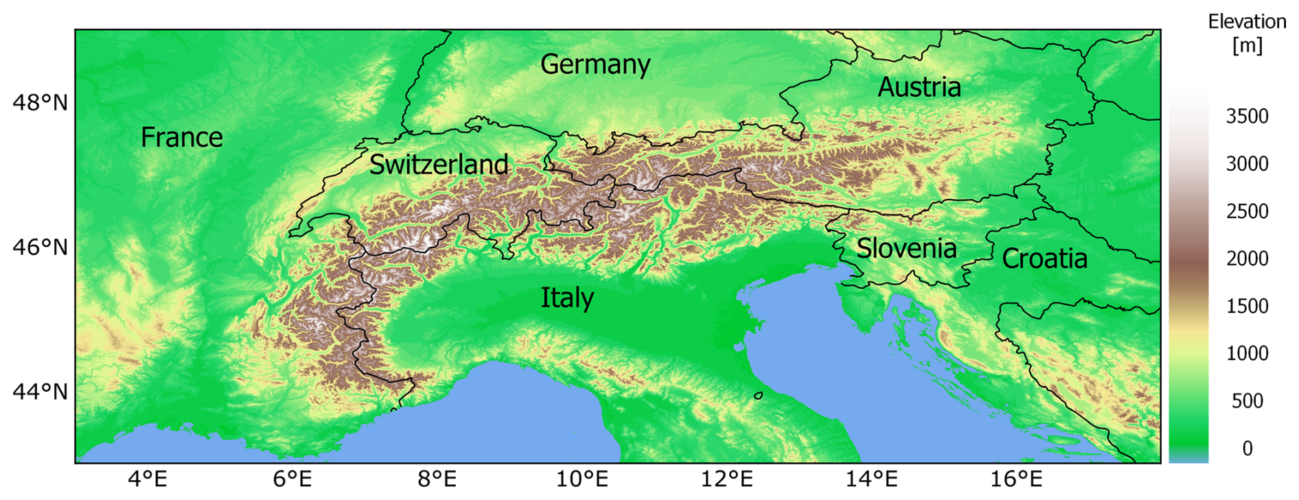
Figure 1 Overview of the Extended European Alpine Region (EEAR). The orography is based on the Copernicus EEA-10 digital elevation model (https://spacedata.copernicus.eu/collections/copernicus-digital-elevation-model, last access: 16 May 2024).

The EEAR is predominantly characterized by complex terrain and, hence, strong elevation gradients, with terrain heights ranging from −5 m a.s.l. (above sea level) at San Giuseppe (Comacchio; Italy) to 4807 m a.s.l. at the top of the Alps at the Mont Blanc summit (Italy–France).

In particular, the EEAR is centered on the European Alps, an arc-shaped mountain range stretching for about 1300 km, delimited to the west by the Bocchetta di Altare (459 m a.s.l.) in northern Italy and to the east by the Godovič Pass (850 m a.s.l.) in Slovenia. Several subalpine mountain ranges surround the Alps, including the Jura Mountains and the Massif Central to the west, the Black Forest and the Bohemian Forest to the north, the Dinaric Alps to the east, and the Apennines to the south. The Alps mountain system, one of the major mountain ranges in Europe, is characterized by diverse climate features influenced by several large-scale weather regimes (Schär et al., 1998; Auer et al., 2005; Panziera et al., 2015). Moreover, the complex topographical features of the Alps and the surrounding mountain chains induce several additional effects on the local climate. These include orographic lifting and the related rain-shadow effect; air channeling and blocking, contributing to phenomena such as föhn winds or thermally driven orographic winds (Serafin and Zardi, 2011; Laiti et al., 2014; Giovannini et al., 2017); and the influence of elevation gradients on temperature patterns (Auer et al., 2007; Marchetti et al., 2017).

Moreover, the southern part of the region stretches into the Mediterranean Sea, another area identified as a climate change hot spot (Hartmann et al., 2013). The presence of these two climate change hot spots, namely the Alps and the Mediterranean Sea, enhances the vulnerability of the region to climate impacts and further motivates the analysis of climatic patterns from observations.

2.2 Data collection

EEAR-Clim includes time series of daily mean, maximum, and minimum air temperature (indicated as T, T_max, and T_min, respectively) and of total precipitation (P). Data were collected from different global, national, regional, and local providers across the EEAR, also exploiting the availability of newly digitized time series. Table 1 summarizes the data providers and the number of stations for each country in the region, the number of time series for each variable, and the starting time of observations.

Table 1 Overview of available stations for each data provider and variable. The “Starting year” column reports the starting year of the series. The “Open data” flag shows whether data are freely available, based upon the provider's policy. Italic font is used to highlight country names.

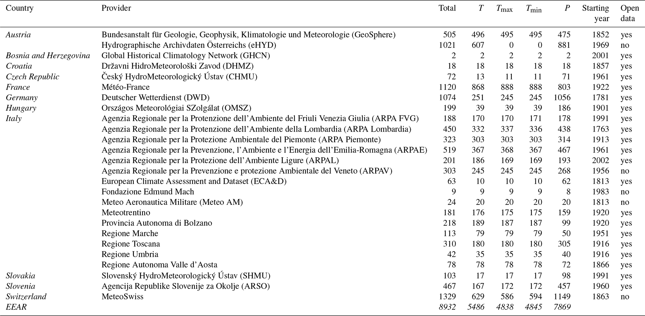
Most of the data are distributed by national providers, except in Italy where meteorological stations are operated by local and regional institutions. Bosnia and Herzegovina faces challenges with respect to the availability of daily climate series due to historical issues related to the dissolution of the former Yugoslavia (Auer et al., 2005). However, a few time series from that country were obtained through the Global Historical Climatology Network (GHCN) (Vose et al., 1992). Figure 2a shows the cumulative distribution of station length with a 10-year resolution, considering all available data from 1870 to 2020. For a few stations, records extend for almost 150 years and date back to the mid-18th century. About 50 % of the available time series measuring at least one variable cover a 30-year time span, long enough to capture key climatological features. Generally, the availability of time series rapidly decays for periods longer than 60 years for air temperature and for periods longer than 90 years for precipitation.

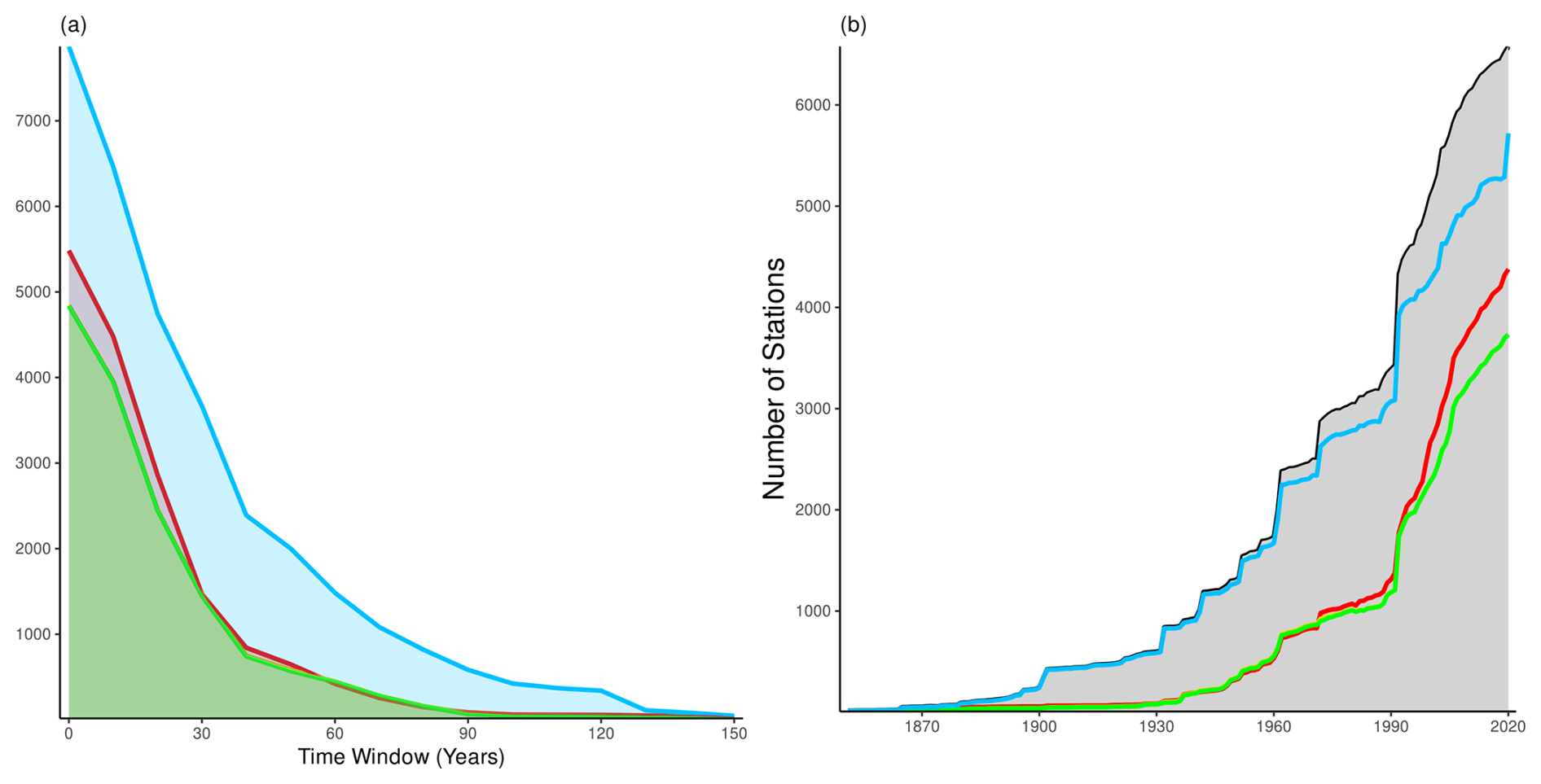
Figure 2 Cumulative distribution of station time series length with a 10-year resolution (a) and histogram of time series (b). Colored lines identify each variable: mean (in red), maximum and minimum air temperature (in green), and precipitation (in light blue). In panel (a), the largest values are the total number of time series, the values for a length of 30 years are the number of stations with at least 30 years of data, etc. In panel (b) the gray shaded area shows the total number of stations with at least one measured variable in the year.

Figure 2b presents a histogram of the available time series, with a 1-year resolution, during the entire observation period, highlighting precipitation as the variable with the largest number of available stations. The sudden increase in station availability from the early 1990s is due to the combined effect of the increasing deployment of new automatic weather stations (WMO, 2008) and the missing digitization of pre-1990 records. Despite the fact that plots in Fig. 2 might suggest that shorter time series cover the most recent period, this is not always true in practice. Indeed, each time series has an independent time extent, leading to a very complex time structure of the dataset, as shown in Fig. A1.

Figure 3a depicts the spatial distribution of stations measuring at least one variable, highlighting the number of nearest neighbors within a 10 km radius and their density vs. elevation. The distance between stations is a useful metric to qualitatively assess the network density, providing an indication of how the densest areas are spatially distributed. The spatial density of weather stations is highly variable during the whole period. However, during the period from 1991 to 2020, the average density is about one station every 6.8 km² – the highest value ever reached by observational datasets over the Alpine region. Switzerland, the northern Apennines, and the main Alpine range are characterized by the highest density of stations, with each of them having at least 10 neighboring stations within a 10 km radius. This high density is more appreciable when compared to other areas, such as the French pre-Alps or the Po Valley. However, the requirement of a minimum density of five neighboring stations within a 10 km radius is met by 70 % of the stations across the whole EEAR. The southeastern part of the domain (Croatia) is the area characterized by the lowest density of stations. This is due to restrictions on local data providers and missing daily measurements. Figure 3b shows the number of stations by elevation and the respective covered area, considering all stations with at least one variable measured and 100 m elevation ranges: more than 50 % are located below 500 m a.s.l., a relatively high percentage (40 %) are located between 500 and 1000 m a.s.l., and about 10 % of stations are located above 1500 m a.s.l. Despite their varying distribution with elevation, the density of stations per unit area in these elevation ranges is comparable, which is in line with the average density over the EEAR.

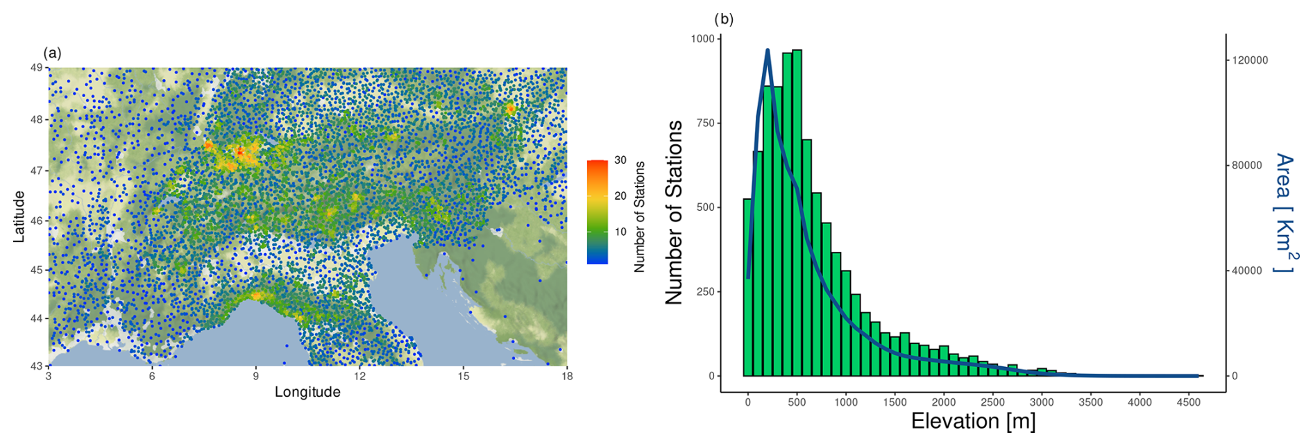
Figure 3 Horizontal and vertical distribution of stations within the EEAR. In panel (a), for each station with at least one measured variable, the color scale highlights the number of nearest neighbors within a 10 km radius. In panel (b), green bars show the number of stations in each 100 m elevation band, while the blue line represents the respective area covered, based on EU-DEM 1.1.

Figure 4 shows the spatial distribution of the stations in the EEAR, highlighting the time coverage, in years, for each station over the measurement period. Clearly, it confirms the abovementioned considerations in terms of inter-station distance (Fig. 3a), but it also highlights some aspects typical of each variable. The higher spatial resolution of the rain-gauge network is evident, as well as the longer time extent of precipitation time series. Air temperature stations show a lower density, particularly in the area surrounding the Alps, such as Germany and Slovenia. Moreover, a different coverage of Austria among the air temperature variables time series is due to the availability of only mean temperature measurements for the eHYD data provider.

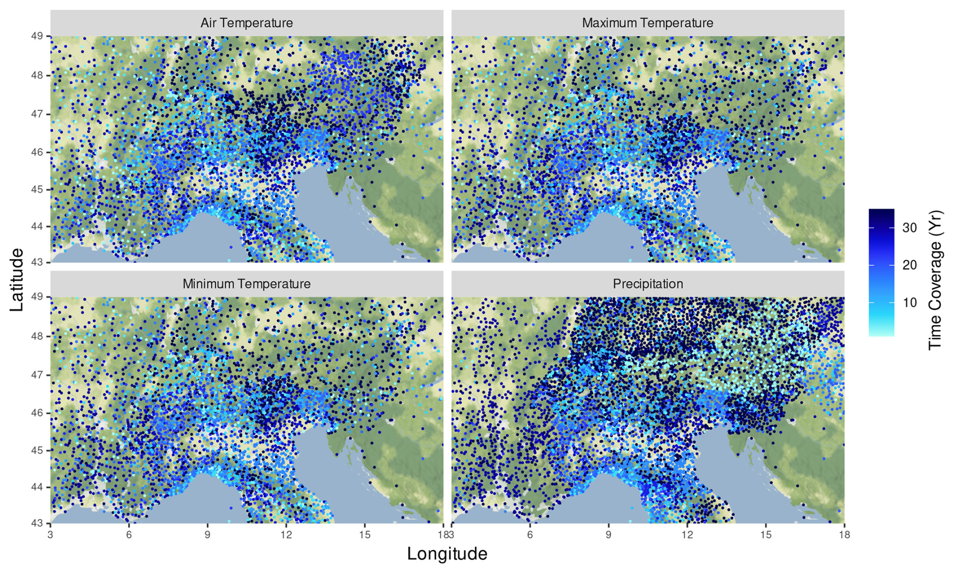
Figure 4 Station distribution for the mean, minimum, and maximum air temperature and for precipitation. The color bar indicates the length of the time series (expressed in years). Time series exceeding 30 years are shown with the same color (the darkest blue).

3 Methods

The twofold QC–homogenization process adopted here involves several steps, illustrated by the flow chart in Fig. 5 and explained in detail in the subsections indicated therein.

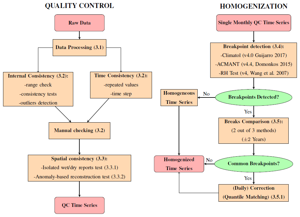
Figure 5 Flow chart of the QC and homogenization procedures. The numbers in parentheses represent the subsections in which the corresponding method is presented.

3.1 Data processing

Data collected from different sources undergo preliminary inspection to identify and address potential issues related to measurement, recording, digitization, transmission, and processing. Data from each source are provided with their own format and peculiarities; hence, initial standardization is essential. Accordingly, data are first converted into a common format, ensuring consistency across the dataset. Proper labeling of missing values is verified by comparing them with quality codes in the metadata when available. Daily time series provided at hourly to sub-hourly temporal resolutions were derived by averaging air temperature data and computing precipitation totals according to the daily period definition adopted by the data provider's procedures. Data are subsequently checked for possible duplicate time stamps and missing dates. Time series shorter than 1 year or without valid data are removed. This preprocessing phase is useful as a preliminary screening before QC procedures. After this stage, stations' metadata are merged into comma-separated value (.csv) files, one for each variable. Each file also includes information about the station name, latitude, longitude, elevation, data provider, country, and a unique alphanumeric code identifying each station.

3.2 Intra-station quality control

Quality control within time series aims at assessing the internal and temporal consistency of time series, following the criteria suggested by the World Meteorological Organization (WMO) (WMO, 2017, 2018), and integrating methods proposed by various authors (Cerlini et al., 2020; Crespi et al., 2018; Curci et al., 2021; Durre et al., 2010; Faybishenko et al., 2022; Fioravanti et al., 2016, 2019; Isotta et al., 2014; Matiu et al., 2021) with new add-ons. The selection and application of these methods depend on the specific variable and its statistical distribution. A summary of the intra-station QC tests is reported in Table 2.

Table 2 A summary of all of the main tests applied to check intra-station consistency.

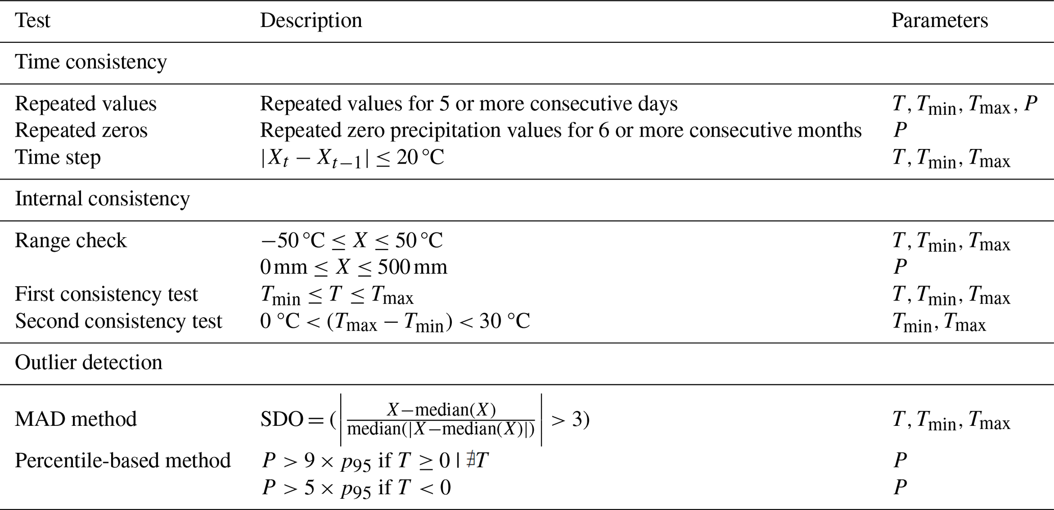
The selected tests are run independently and automatically, generating flags for each observation to highlight anomalous values saved in log files. Abnormal values are manually inspected in a conservative way, i.e., flagging only the values that are definitely erroneous as missing values. In these cases, the decision is supported by information available from meteorological archives and the agreement among quality flags. The time consistency check examines the rate of change in data over time through two tests. The repeated-values test inspects sequences of identical readings prolonged for more than 5 d, which is crucial for identifying data entry errors. In the case of precipitation data, extended sequences of 0 mm, possibly due to erroneous transcription of missing data (Peterson et al., 1998), are identified and replaced with missing value flags if they exceed 180 d. In addition, a step check is applied to air temperature data, comparing consecutive temporal changes to the step limit value of 20 °C, equal to the maximum permitted day-by-day variation. This ensures that sudden, unrealistic jumps in temperature readings are flagged and reviewed for data quality issues.

The internal consistency tests aim to identify major errors in time series from inspections of data within reasonable ranges. In particular, the range check evaluates whether daily measurements fall within physically consistent ranges based on historical records (WMO, 2017). Air temperature data are validated against extreme values of −50 °C, close to the minimum record of −49.6 °C on 10 February 2013 in Busa Fradusta (Pale di San Martino group, Italy), and 50 °C, which includes the highest record of 45.9 °C on 28 June 2019 in Gallargues-le-Montueux (France). Similarly, the highest record of 948.4 mm, recorded on 7 October 1970 in Bolzaneto (Genoa, Italy), is considered in setting precipitation thresholds. However, because of uncertainties related to precipitation measurements, conservative thresholds of 0 and 500 mm are set.

Consistency check tests assess the relationship between two or more parameters, comparing observations to evaluate physical and climatological consistency (WMO, 2017). Specifically, two consistency checks compare mean, maximum, and minimum air temperature: one evaluates whether the mean temperature falls between its minimum and maximum daily values, whereas the other method focuses on the difference between minimum and maximum temperatures, evaluating whether it is nonzero and within a given threshold, set at 30 °C, to capture realistic temperature variations. Data corruption or measurement errors can produce outliers, i.e., observations that significantly deviate from the others (Aggarwal, 2017; Hawkins, 1980). Outlier detection is aimed at identifying statistical anomalies within the distribution of time series values, and it is the test that requires the most careful attention. Thus, an ex post manual verification is always recommended.

In the literature, the mean and standard deviation are indexes conventionally used to detect outliers, assuming a normal distribution of data. However, the presence of outliers and skewed data distributions can compromise the effectiveness of these two metrics. A typical solution to address the issue of skewness is data symmetrization, such as the application of a Box–Cox transformation (Rayens and Srinivasan, 1991), although this method may not reliably identify outliers. A more robust alternative for outlier detection is the use of the median and the median absolute deviation (MAD). Indeed, the median is less sensitive to the presence of outliers (Leys et al., 2013; Hunziker et al., 2018), and it can be easily adapted to skewed distributions without losing robustness (Meropi et al., 2018). In this study, outliers of air temperature data are detected using the median and MAD, as suggested by Leys et al. (2013). Thus, the Stahel–Donoho outlyingness (SDO) measure (Pavlidou and Zioutas, 2014) is adopted. Using this measure, an outlier is detected if the SDO value exceeds a predefined threshold of 3, according to a conservative outlier removal (Miller, 1991). In the case of precipitation data, detection methods often rely on upper percentile-based thresholds (Cerlini et al., 2020). Here, we consider two different thresholds, 5 and 9 times the 95th percentile, respectively, contingent upon the availability and the sign of air temperature data for the tested time series.

3.3 Study of spatial consistency

After intra-station QC, the resulting time series undergo fully automatic spatial consistency tests, and data flagged with warning flags are automatically replaced with missing values. The spatial consistency tests are crucial, as they identify further inconsistencies that were not detected by previous checks. The tests compare the records of each time series, called target stations, with those of nearest neighbors, called reference stations. However, when daily time series of different stations are compared, the issue of time shifting may arise. Indeed, observational times may differ among different stations and data providers, especially for precipitation data, hindering the comparability of daily records (Schmidlin et al., 1995; Kunkel et al., 2005; Reek et al., 1992). The time-shifting issue is faced by a 3 d moving-window comparison, i.e., each daily value in the target station is compared to those of neighboring stations on the previous, current, and next day. Thus, this approach effectively addresses potential time shifts in the assignment of 24 h accumulated rainfall, providing robust results, even in cases of partial overlap between target and reference data.

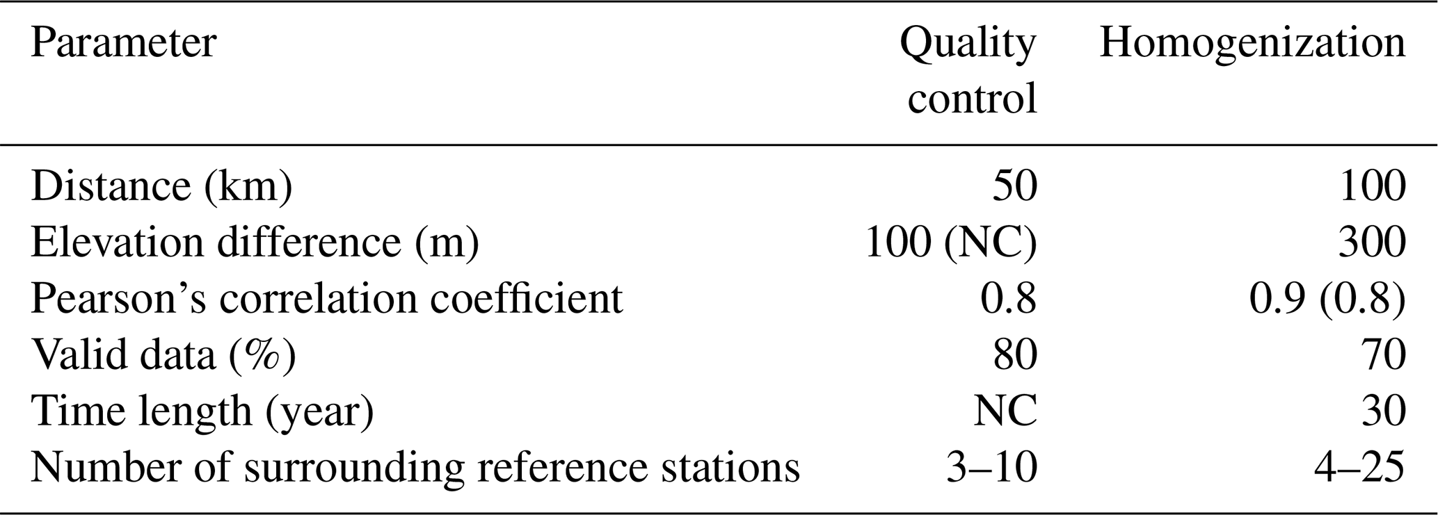
Before the application of the tests, candidate reference stations are selected based on specific criteria outlined in Table 3. Only stations within a 50 km radius around the target station are considered. In the case of air temperature time series, stations with an absolute elevation difference exceeding 100 m are rejected. Further selection criteria include a Pearson correlation coefficient threshold of 0.8 and a maximum allowable missing data percentage of 20 % over the common period with the target station (Alexander et al., 2006; Toreti and Desiato, 2008). Typically, a set of a minimum number of 3 and a maximum of 10 reference stations is identified for each target station. When a set includes more, only the closest 10 are retained. Conversely, if fewer than three candidates meet the criteria, no test is applied.

Table 3 Overview of parameters used to select reference time series for spatial QC and break point detection. Geographic distance, in kilometers, between station points is computed by the geosphere R package (Hijmans et al., 2021). The elevation difference parameter, expressed in meters, is used to reject candidate stations located at elevations too different from the target station. The number of surrounding reference stations defines the lower and upper limits of candidate stations that can be selected. Values in parentheses show the specific thresholds used for precipitation data. Values labeled with “NC” refer to parameters not considered when selecting reference time series.

3.3.1 Wet and dry isolated reports test

This test is applied solely to precipitation time series, following Isotta et al. (2014). The main goal is to assess whether wetness or dryness daily conditions observed at the target station are corroborated by the reference time series. The distinction between wetness and dryness depends on whether the total precipitation exceeds a given threshold, defined as in Isotta et al. (2014). Wetness conditions at the target station are defined when the daily precipitation amount exceeds a threshold depending on the distance between the target and the closest reference station, as well as the period of the year. The threshold is computed as follows:

$$\begin{array}{}\text{(1)}& {\mathrm{th}}_{\mathrm{p}}=f_{\mathrm{wd}}+f_{\min }{\displaystyle \frac{d_{\min }}{d_{\mathrm{th}}}},\end{array}$$

where d_min is the distance between the target and reference station; d_th is the distance threshold, here set to 15 km (Isotta et al., 2014); and f_min and f_wd are constants, both expressed in millimeters. The test is applied only if d_min does not exceed a tolerance value equal to d_th. However, during the convective season, from May to September, the tolerance value is increased to 20 km to account for the higher variability associated with that season, although d_th remains unchanged. The constants f_min and f_wd have respective values of 3.2 and 0.3 mm during the convective period or respective values of 2.7 and 0.3 mm otherwise. The test confirms wetness conditions at the target station if at least one reference station records a precipitation amount higher than 0.3 mm within a 3 d moving window centered on the tested day.

The procedure for testing dryness conditions mirrors the wetness case but with reversed thresholds. According to Isotta et al. (2014), dry conditions at the target station are defined when the daily precipitation amount is below 0.3 mm. For the reference stations, the threshold is computed using Eq. (1) but with f_wd increased to 0.8 mm. The test confirms dryness conditions at the target station if, within the same 3 d moving window, at least one reference station records a precipitation amount lower than 0.3 mm. When isolated dry or wet conditions are detected, the respective values at the target station are flagged as missing data.

3.3.2 Anomaly-based tests

Anomaly-based tests focus on climatological anomalies, i.e., deviations of observed data from their long-term average. These tests are applied to the time series of all the variables including at least 30 years of data. The selected reference time series are limited to the time extent of the target station. The resulting set of time series is used to compute a daily climatology by averaging the values over all years and using a moving window centered on the considered day. The window length depends on the variable considered. In the case of air temperature, a 15 d moving window is used, whereas for precipitation, zero values are excluded and the window length is increased to 30 d. The daily climatology is computed using the ts2clm function from the heatwaveR R package (Schlegel and Smit, 2021). Finally, daily anomalies from climatologies are computed for each target station.

The first test, known as the corroboration method, follows Durre et al. (2010) and Curci et al. (2021). Anomalies at the target station are compared to those at the reference stations using a 3 d moving window centered on each day, assessing whether the discrepancy is below a given threshold for at least one reference station. The threshold is determined through sensitivity tests on raw time series, aimed at finding the optimal value that allows both the successful detection of previously identified outliers and the reduction of false outlier flagging. The selected value is set at 10 °C for air temperature and at 50 mm for precipitation. If the target station anomaly is not corroborated by any reference time series anomalies, the daily value is flagged as an outlier. An additional control for precipitation data consists of computing the relative difference between target and reference time series anomalies. If the relative error exceeds 50 %, the suspicious anomalous values are labeled as outliers.

The second test, based on methods suggested by Matiu et al. (2021) and Crespi et al. (2018), reconstructs target station values averaging the quantities x_r,j computed for each reference station j:

$$\begin{array}{}\text{(2)}& x_{r,j}=x^{\prime }+y_{\mathrm{anom},j}-x_{\mathrm{anom}},\end{array}$$

where x_anom and y_anom,j are the anomalies of the target and reference station j, respectively, computed following the same procedure as the corroboration method. Here, x^′ denotes the target station time series with missing values reconstructed from neighboring stations using a spatial interpolation approach:

$$\begin{array}{}\text{(3)}& x_i^{\prime }=\left\{\begin{array}{ll}\frac{{\sum }_j{w}_j\left(x_{i,j}+\cdot {\mathrm{cf}}_j\right)}{{\sum }_j{w}_j}& \text{if}{x}_i=\mathrm{NA}\\ x_i& \text{otherwise}.\end{array}\right.\end{array}$$

Here, x_i,j represents the data from reference time series j for day i, and w_j represents the weights and is defined as follows:

$$\begin{array}{}\text{(4)}& w_j=e^{-\frac{\left(\mathrm{1}-{r_{ij}}^{\mathrm{2}}\right)}{\frac{{\mathit{\tau }}_r^{\mathrm{2}}}{{\log }_{\mathrm{2}}}}},\end{array}$$

where r_ij is the correlation coefficient between the target i and reference station j, and τ_r is a constant equal to 0.3. In Eq. (3), cf_j is the correction factor, relating the target and reference series based on their climatological conditions. For precipitation, cf_j is the ratio of the averages of daily data between the target (excluding the daily record under reconstruction) and the jth reference time series. For air temperature, cf_j is the difference between these averages. The correction term $x_{i,j}+\cdot {\mathrm{cf}}_j$ means $x_{i,j}\cdot {\mathrm{cf}}_j$ for precipitation and $x_{i,j}+{\mathrm{cf}}_j$ for air temperature. Finally, the original x and reconstructed x_r,j time series are compared using the same twofold procedure as the corroboration test. This includes the application of the 3 d moving-window comparison and, for precipitation data, the assessment of whether the relative difference between x and x_r,j is below 50 %.

3.4 Break detection methods

The high density of the dataset allows for a robust assessment of time series homogeneity. However, when dealing with a large number of time series, homogenization has to be carried out by selected automatic methods. Although an unsupervised homogenization procedure is not recommended (Aguilar et al., 2003), its implementation is now quite common (Ribeiro et al., 2016), as most methods exploit iterative intercomparisons of several nearby and correlated stations (Curci et al., 2021). The application and comparison of different algorithms is strongly suggested (Toreti et al., 2011; Kuglitsch et al., 2012; Ribeiro et al., 2016; Brugnara et al., 2023), particularly if station metadata are not available. This approach reduces false break detection and increases confidence in accepting or rejecting break points. Another issue related to dataset homogenization is the quantity of computational resources required. In this respect, the best solution is to run break detection methods on single stations to optimize the process – i.e., to reduce the computational load and increase the reliability of detected inhomogeneities.

The selected methods for break detection have to be accurate and reliable in detecting break points; permit running in automatic mode, given the large number of stations; tolerate missing values without limitations; and allow the homogenization of time series without restrictions with respect to time or quantity. After careful comparisons among the various options offered in the literature, for the purpose of the present work, we adopted three automated methods satisfying the above conditions, namely Climatol, ACMANT, and the RH test.

Climatol is a relative homogenization method based on the standard normal homogeneity test (SNHT) (Alexandersson, 1986), available as an R package (Guijarro, 2023). In Climatol, a break point is detected if SNHT statistics returns a value over a given threshold. Here, the default SNHT threshold of 25 is used for air temperature. For precipitation, following Guijarro et al. (2023), we set a lower value of 15, given the higher variability in precipitation and the greater difficulty in detecting inhomogeneities.

ACMANT (the adapted Caussinus–Mestre algorithm for the homogenization of networks of climatic time series; Domonkos, 2015 and Domonkos and Coll, 2017b) is a fully automated method, inheriting the detection process from the PRODIGE method (Caussinus and Mestre, 2004). The number of breaks is estimated with the Caussinus–Lyazrhi criterion (Caussinus and Lyazrhi, 1997), and inhomogeneous periods are corrected using the analysis of variance (ANOVA) method. When run in automatic mode, ACMANT requires a set of input parameters and settings concerning outlier filtering, the output format, and the snow season period for precipitation. Here, the snow season is set from November to May, the output files are kept in the default format, and the program is run ignoring outlier filtering, as outliers are already removed during the QC process described in the previous sections.

The third method that we adopted is the RH test (Wang, 2008), suggested by the Expert Team on Climate Change Detection and Indices (ETCCDI; https://etccdi.pacificclimate.org/, last access: 15 October 2024). This method detects break points using a penalized maximal t test and requires a reference time series provided by the user, unlike other methods. Here, reference time series x_ref are computed as the weighted mean of candidate references x:

$$\begin{array}{}\text{(5)}& x_{\mathrm{ref}}={\displaystyle \frac{{\sum }_j{w}_j{x}_j}{{\sum }_j{w}_j}},\end{array}$$

where w_j are the weights, computed as in Eq. (4). Detected break points in a time series must all be significant. If they are not, the program should be rerun after removing nonsignificant break points, and the procedure has to be repeated until all the detected break points are labeled as significant.

The above methods are among those ranked best in comparative studies of different homogenization approaches, such as the MULTITEST project (Domonkos and Coll, 2017a; Guijarro et al., 2023). Their use is documented in several studies concerning different climate variables (Luna et al., 2012; Mamara et al., 2013; Azorin-Molina et al., 2016; Chimani et al., 2018; Hunziker et al., 2018; Squintu et al., 2019; Brugnara et al., 2023). Additionally, all three methods have a high tolerance for missing values.

3.5 Detection of inhomogeneities

All of the above methods employ a relative break point detection approach, i.e.,  using information from a set of neighboring stations. Homogeneity methods are run on single time series, which are aggregated monthly, with at least 30 years of data and 70 % of valid observations (Wijngaard et al., 2003). These conditions are also adopted when selecting the set of reference stations for the homogenization process, as reported in Table 3. Reference stations are further selected based on horizontal distance, elevation difference, and time correlation, as reported in Table 3. Specifically, reference stations must be located within a horizontal radius of 100 km centered on the test station. An elevation difference threshold of 300 m was chosen, a value included within the range of 200–500 m commonly adopted in the literature (e.g., Buchmann et al., 2022). Reference time series are further selected based on the Pearson correlation coefficient of first differences, compared to the tested time series. The coefficient is required to be no smaller than 0.9 (Kunert et al., 2024). If no reference station meets this threshold, a time correlation of at least 0.8 is accepted. In case of precipitation, the thresholds are 0.8 and 0.7, respectively. Homogeneity is tested if at least four reference stations can be found. The maximum number of reference stations is set to 25 as an optimal compromise between the reliability of the procedure and a reasonable computational time for the homogenization process. When this threshold is exceeded, only time series with a higher percentage of valid data are retained.

Homogenization results obtained by the three methods are analyzed to identify time series requiring corrections as affected by one or more break points (Fig. 5). The assessment of break point significance is based on cross-comparison among candidates identified by more than one method to minimize false positives. Hence, following Buchmann et al. (2022), a break point is considered significant if at least two methods detect it within the same time window, with a tolerance of ±2 years. However, break points in the first and last 2 years of the series are rejected because all methods typically struggle with interpreting changes occurring either at the beginning or the end of time series (Ducré-Robitaille et al., 2003; Resch et al., 2023). In addition, if multiple break points are detected in the same time series within a 2-year period, only the most significant is retained based on the SNHT and RH test results.

In view of determining the minimum number of methods required to identify a break as valid, a sensitivity study was performed. Two configurations were considered: one with all three methods detecting a given break point (named Exp 1) and another with two out of three methods detecting it (Exp 2). Exp 1 is more restrictive than Exp 2, requiring an agreement among all methods, which is more difficult to attain given the different performance of each algorithm (Guijarro et al., 2023). Note that the Exp 2 configuration closely follows the procedure applied by Brugnara et al. (2023). The results were then compared with a composite set of homogenized time series provided by Météo-France, MeteoSwiss, and HISTALP (Auer et al., 2007; Chimani et al., 2023). Exp 1 turned out to be too restrictive, identifying only a low percentage of inhomogeneous time series (about 10 % for precipitation and 26 % for temperature). Exp 2 showed an agreement 3 times higher than Exp 1 and is therefore adopted here to identify inhomogeneous series.

3.5.1 Homogenization

Inhomogeneity in time series related to non-climatic factors generally gives rise to unrealistic oscillations, which lead to underestimation and the reduced spatial coherence of long-term trends, and erroneous high variability in climate anomalies (Begert et al., 2005; Curci et al., 2021; Brugnara et al., 2023; Guijarro et al., 2023). The adjustment of inhomogeneous time series before their use is then mandatory to provide reliable results of climate analyses.

Here, time series affected by significant break points are corrected by applying adjustments to each daily value, calculated from monthly corrections. Inhomogeneous data are corrected conservatively, i.e., data are adjusted only for periods of evident inhomogeneity. The method used to correct inhomogeneous time series is the quantile-matching technique proposed by Squintu et al. (2020). This method applies adjustments of different sizes depending on the magnitude of the value to correct. Thus, as noted by Brugnara et al. (2023), this approach allows for a more robust correction of extreme records compared to methods applying the same adjustment to all dates regardless of the recorded intensity. Our approach differs from the original method suggested by Squintu et al. (2020) in the selection of reference stations and applies only one iteration of the original algorithm, in agreement with the conservative approach adopted for break point detection. The selection of the reference stations follows the procedure already used for the detection of break points, but here no limitation is set on the maximum number of candidate stations. However, the method was designed mainly for temperature data. For precipitation, suitable modifications were introduced (see Appendix B for further details). After making corrections, quality control is carried out by applying the range test to evaluate if adjusted data were still physically consistent. If the corrected values do not pass the test, the correction is rejected and the original values are kept. Consistency tests were also applied to temperature data. First, minimum and maximum temperatures were compared to evaluate if T_min≤T_max; if this was not the case, they were set as equal. Then, the relationship $T_{\min }\le T\le T_{\max }$ was assessed. If mean temperature data did not satisfy this condition and both minimum and maximum temperature time series were available, T data for the whole time series were computed as the average of T_min and T_max. When only minimum or maximum temperature data were available, T data that did not pass the test were set equal to T_min or T_max.

4 Results and discussion

4.1 Quality control

The results of the QC procedure for mean air temperature and precipitation are summarized in Table 4 by data provider. Results are shown in terms of the percentage of missing values before QC, flagged values after the two steps of QC, the interquartile range (IQR) of flagged values, and valid data after the QC procedure. On average, the percentage of flagged values is below 1 % for mean temperature data. For precipitation, the average value is higher, more than 3 %, largely due to the very high percentage of flagged values for ECA&D data, with percentages still exceeding 1 % in a few other cases, such as data from Lombardy (ARPA Lombardia) and South Tyrol (Provincia Autonoma di Bolzano). Air temperature time series are affected by non-negligible quality issues, concerning stations mainly located in Emilia-Romagna (ARPAE), for mean temperature, and Lombardy, for minimum and maximum temperatures. Data providers with high percentages of flagged values also exhibit a high IQR, suggesting that average statistics for these providers are affected by the poor quality of isolated time series.

Table 4 Summary of results after the QC process for air temperature and precipitation. Each column shows, for each data provider, the percentage of missing data in the raw time series (Miss); flagged values in time for the internal and outlier detection phase of quality control (Base QC); flagged values during the application of spatial tests (Space QC); the interquartile range (IQR) of total flagged values (QC IQR); and valid data at the end of the process (Valid). Italic font is used to highlight country names.

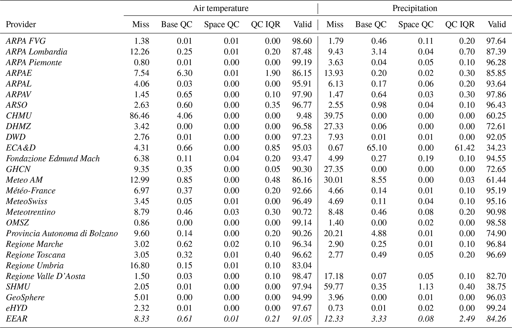
The final percentage of valid data after QC is, on average, above 90 % for mean temperature and 80 % for precipitation, indicating an overall good quality for most of the periods included in the dataset. Indeed, 90 % and 75 % of the total missing data at the end of the QC process for air temperature and precipitation, respectively, were already missing in the raw time series. Data providers exhibiting the lowest percentages of valid measurements are primarily located near the domain borders, such as the Czech Republic (CHMU) and Umbria (Regione Umbria, Italy). However, a larger number of precipitation series and the extended length of these series increase the likelihood of detecting missing or no valid data. This observation is supported by two statistical insights: (1) the number of valid data in precipitation time series is twice as high as that of air temperature, and (2) the density of time series with minimal or no missing data is higher for precipitation than for temperature (Fig. A2). Thus, the removal of about 0.62 % of air temperature and 3.41 % of precipitation issues, on average, and the marginal influence of data removal on the number of valid observations demonstrate that the QC process clearly improved the overall accuracy of the dataset.

4.2 Homogenization

Figure 6 shows the distribution of break points from 1961 to 2020 for precipitation and for the minimum, mean, and maximum temperature. Each series cannot include more than one break point per year, allowing us to express the incidence of inhomogeneities as a percentage of the total number of series available each year. The most prominent peak, observed around the early 1990s, is consistent across all temperature variables and reflects the transition from mechanical to automatic weather stations. A smaller peak in the mid-2000s corresponds to the installation of technologically advanced automatic stations, i.e., newer stations equipped with improved shielding and ventilation systems designed to overcome the issue of temperature overestimation caused by radiation effects (Böhm et al., 2001; Aguilar et al., 2003; Venema et al., 2013). Another notable peak, which is more pronounced in the mean and minimum temperatures, occurs in the early 1980s. In contrast, the distribution of precipitation break points does not clearly indicate periods of measurement changes, likely due to fewer detected break points.

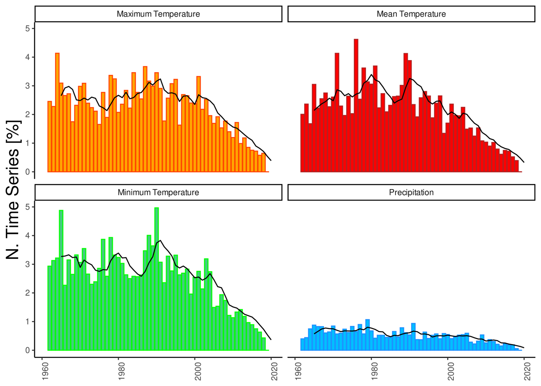
Figure 6 Histogram showing the time distribution of detected break points for the 1961–2020 period, expressed as the percentage of stations with respect to their total number. The black line represents the 5-year moving-window average.

Inhomogeneous time series account for about 20 % of air temperature records (18.3 %, 21.6 %, and 20.6 % for mean, minimum, and maximum temperature, respectively), whereas they are less common for precipitation (i.e., 12 %) (see Appendix A). This lower incidence in precipitation series may be attributed to the greater difficulty in detecting break points in these time series, which are well known to typically suffer from higher noise levels (Gubler et al., 2017), stemming from the spatial and temporal variability in precipitation measurements as well as from the complexity involved with accurately measuring precipitation under different environmental conditions (Peterson et al., 1998). Although the overall number of break points detected in the air temperature time series is similar, their distribution among data providers, shown in Fig. 7, is more variable. Stations located above 2000 m a.s.l. generally exhibit higher homogeneity (see Appendix A), likely due to fewer time series that are either too short or lack sufficient references for homogeneity testing. The percentage of time series that cannot be tested due to inadequate reference stations is negligible, typically ranging from 0.1 % to 0.2 %. These situations are primarily associated with very high elevation sites or regions near domain borders with a lower station density.

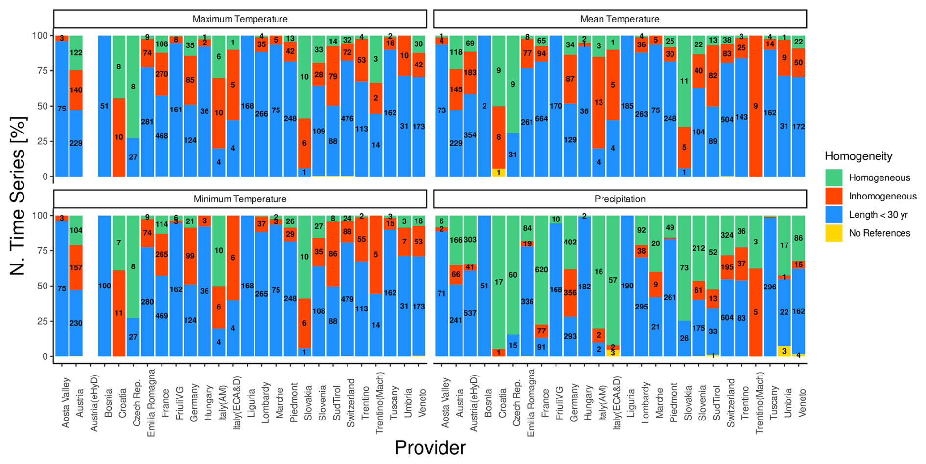
Figure 7 Distribution of homogeneous time series (green), inhomogeneous time series (red), insufficiently long time series (blue), and time series lacking reference stations (yellow) based on the data provider for the mean, minimum, and maximum air temperature and for precipitation. The y axis indicates the percentage of stations in each category, while labels within bars show the absolute numbers of stations.

Figure 8 shows box plots of the mean daily adjustments applied to each inhomogeneous time series for temperature (mean, maximum, and minimum) and precipitation by the data provider. Providers whose time series are not affected by inhomogeneities or whose time series require minimal corrections are omitted. Average daily adjustments generally center around zero, and fall within a ±2 °C range for air temperature and a ±10 mm range for precipitation. However, corrections exceeding these ranges are present, albeit infrequently, as outliers in box plots for some data providers. France (Météo-France), Lombardy (ARPA Lombardia), and Slovenia (ARSO) show a higher prevalence of time series requiring non-negligible corrections for both air temperature and precipitation.

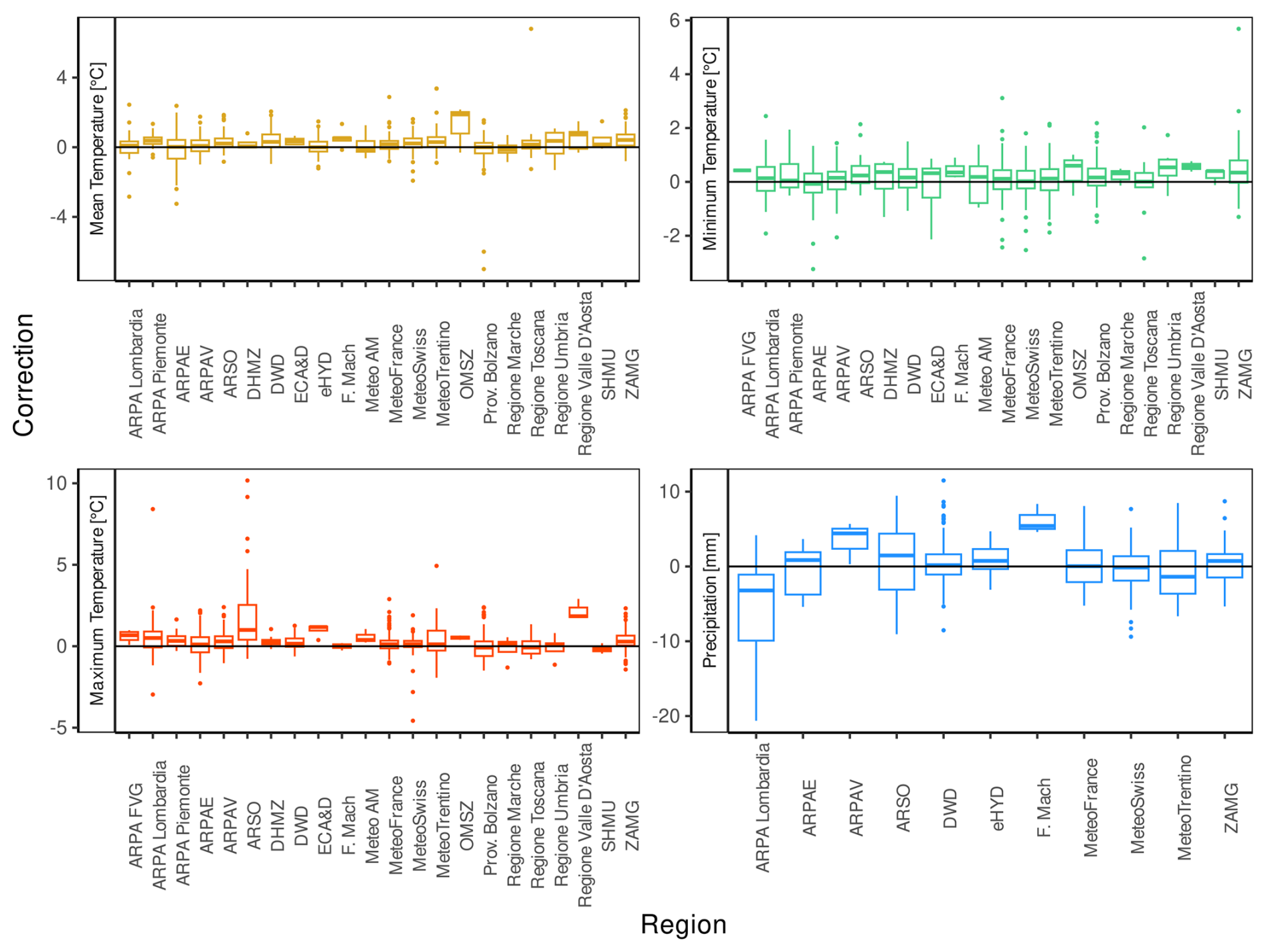
Figure 8 Box plots of mean daily adjustments for each inhomogeneous time series by data provider. Each box includes data within quartiles, and the central line shows the median. Data outside the box but within 1.5 IQR are represented by upper and lower whiskers. Data exceeding these thresholds, i.e., outliers, are shown as points. A black line indicates a situation in which no correction is required.

4.3 Dataset features and user guide

The new and unprecedented EEAR-Clim dataset developed in this study features key properties that are different from the state of the art for similar station-based observational products in terms of quality, space–time resolution, and completeness. Quality improvements, attained through the application of an extensive and accurate procedure, and the increased resolution in time and space are expected to provide a more realistic representation of environmental conditions. This has the potential to positively affect the accuracy of hydroclimatic predictions and enhance the reliability of bias-corrected model data (Laiti et al., 2018). Moreover, a more realistic understanding of climate variables plays a key role in improving our knowledge of the Alpine climate state and its variability (Hartmann et al., 2013; Begert et al., 2005; Skrynyk et al., 2023).

A quantitative comparison of EEAR-Clim with other existing observational products covering the Alpine region, such as APGD (Isotta et al., 2014), E-OBS (Cornes et al., 2018), and HISTALP (Auer et al., 2007), is challenging due to the different types (e.g., station archives and gridded datasets) and purpose of the datasets. However, a qualitative assessment of strengths and weaknesses can provide valuable guidance for potential dataset users. The EEAR-Clim dataset significantly increases the spatial coverage in terms of available time series by more than 30 %, compared to those used in the interpolation of gridded datasets like APGD and E-OBS, allowing for an improved representation of the orographic effects. The higher spatial density also allows for an enhanced representation of climate variability with elevation. Indeed, comparing the density of stations in different altitudinal ranges, we found similar values converging to an average density of about 1.5 stations every 10 km², implying a rather homogeneous distribution of observations across elevation ranges. A reliable comparison in terms of elevation distribution with other products cannot be easily achieved: the strong decay of available observations at higher elevations is widely known (de Jong, 2015).

The multiparameter feature of our dataset is rare to find in high-resolution observational products. Although E-OBS and HISTALP already include meteorological data of several variables, the collection of such a large number of multiparameter observations at a daily resolution is really unprecedented and can enhance an integrated assessment of Alpine climate changes based on a better understanding of interactions between the different variables (Brunetti et al., 2009; Gaffen and Ross, 1999; Kaiser, 2000; Wang and Gaffen, 2001; Huth and Pokorná, 2005; Beniston, 2006). Another key strength of EEAR-Clim is its rigorous approach to addressing data quality issues. Indeed, despite the fact that a quality check is commonly performed for other observational datasets, the level of detail applied in EEAR-Clim is notably higher. Furthermore, the homogenization of high numbers of time series over large domains, such as the EEAR, is a task rarely performed with the high degree of robustness provided here. Among other datasets considered, E-OBS and APGD do not homogenize time series. Overall, our efforts aimed to homogenize two-thirds of the air temperature and one-fourth of the precipitation time series, strongly reducing the heterogeneity of the dataset. The exclusion of time series shorter than 30 years from the homogenization procedure, in line with the standard practices (Wijngaard et al., 2003), prevents the introduction of further uncertainties or algorithm artifacts and, thus, enhances the dataset accuracy.

Our collection efforts also resulted in gathering observations with enough temporal coverage. About 30 % and 47 % of the respective air temperature and precipitation time series consist of at least 30 years of data. A considerable number of time series, 15 %–25 % (∼ 1500–2000) depending on the variable, cover a period of 60 years or more, with about 5 % (∼ 600) of observations extending up to a century, despite the fact that many historical records are currently unavailable in digital form. Although most time series are relatively shorter compared to historical products such as HISTALP, EEAR-Clim provides unique station-level detail without sacrificing the temporal extent. Other products show a comparable time extent (such as E-OBS) or a shorter time extent (APGD) compared to EEAR-CLIM, but they lack the finer spatial detail preserved here.

All time series in the dataset can be used to study climate variability, keeping in mind that time series shorter than 30 years may include potential inhomogeneities. However, the inclusion of about 1600 homogenized temperature series and 4000 homogenized precipitation series longer than 30 years provides a robust foundation for assessing climate trends, representing a significant data availability enhancement compared to earlier studies. Users should also pay attention when time series in different areas or at different elevations are compared, due to the different techniques and procedures adopted by data providers. This especially involves mean temperature, which might be derived by employing different approaches (Baker, 1975; Weber, 1993; Weiss and Hays, 2005; Villarini et al., 2017), and high-elevation precipitation measurements, whose reliability mostly depends on, among others, the availability of heated rain gauges or equipped with a wind deflector. The limited access to the metadata of all stations included in the dataset makes it impossible to systematically identify all of these differences. However, the computation of daily mean temperature from hourly values, when possible, and the robust quality control procedure applied reduced these discrepancies among data providers, thereby enhancing data confidence.

Different historical data digitization initiatives are underway; thus, the dataset can be further expanded (also beyond the last 60 years) in terms of data coverage. Future research activities could be dedicated to improving the EEAR-Clim dataset and including measurements of other essential climate variables, thereby further enriching its utility for integrated climate assessments. Despite these possible further updates, making the dataset operational requires funded and permanent projects, open-access data frameworks, and supportive European policies. Given the resources and coordination required, a similar initiative, typically undertaken by climate services, is outside the scope of our current academic framework.

5 Code and data availability

All computations were performed with version 4.2.1 of the R statistical software (R Core Team, 2022). The code is available from a repository, including the main scripts to read and process data, perform quality control, and perform the main tasks of homogenization. Most of the contributing institutions agreed to share their data (see Table 1). Hence, the open data are available from the Zenodo repository (https://doi.org/10.5281/zenodo.10951609, Bongiovanni et al., 2024) as separated raw, quality-checked, and homogenized time series. For the full dataset, including undisclosed data, please contact the corresponding author.

6 Conclusions

A new observational dataset of air temperature and precipitation at a daily resolution for the Extended European Alpine Region (EEAR), covering the whole available period of measurements, has been presented. The data collection effort resulted in a very high spatial density and led to a homogeneous regional coverage. This achievement was favored by newly digitized data and the collection of datasets from national, regional, and local institutions. The EEAR-Clim dataset includes most of the available stations in the EEAR, managing to increase the density, even at higher elevations, which is a typical issue of observational datasets in topographically complex regions. Furthermore, collecting data from multivariable measurements and including the most recent records (updated to the year 2020) are important add-on improvements compared to other available products for the area. Here, the dataset consists of air temperature and precipitation data, but the release of an updated version also including additional variables is planned. Substantial efforts were made to ensure the consistency and quality of the different data contributions. A deep and extensive quality control was carried out, following WMO criteria in terms of data quality (WMO, 2017), merging different approaches and integrating new techniques aimed at facing all critical issues of rescued data. The QC procedure flagged about 5 % of total observations, of which 80 % are precipitation data. While QC did not significantly affect the number of valid data, which is about 90 % on average, it improved the overall accuracy. A tailored homogenization procedure was performed on quality-checked data. The break detection stage was based on three automatic methods: Climatol, ACMANT, and the RH test. The comparison of results provided by these independent procedures ensures reliable identification of significant change points, especially when metadata are not available (Fioravanti et al., 2019). Inhomogeneous time series with identified break points were homogenized using the quantile-matching algorithm, applying adjustments depending on percentiles of the empirical distribution. The inhomogeneities detected in precipitation time series are fewer than those identified in temperature time series, as also reported in other studies (Gubler et al., 2017; Skrynyk et al., 2023). The increased homogeneity at elevations above 2000 m a.s.l. could be explained by external factors (e.g., a reduced sample of stations) rather than specific accuracy of high-elevation time series. Break point detection results and adjustment magnitudes were in agreement with other existing studies focused on areas including the EEAR or its subregions (Brugnara et al., 2023; Squintu et al., 2020; Mamara et al., 2013; Coll et al., 2020). A subset of the time series covering the 1961–2020 period was used as a basis to carry out an extended analysis of trends and climate features of both average values and extremes (Bongiovanni et al., 2025). Additionally, a high-resolution gridded version of the EEAR-Clim dataset is planned for release. These subsequent analyses and applications highlight the relevance of the new observational dataset developed in this work as a tool for better understanding Alpine climate changes over recent decades and improving the reliability of model simulations and future scenarios. The procedure developed within this work can be readily implemented over other areas or time periods; adapted to time series at different time frequencies; and extended to other variables, such as relative humidity, wind speed, solar radiation, or snow depth.

Appendix A: Additional material

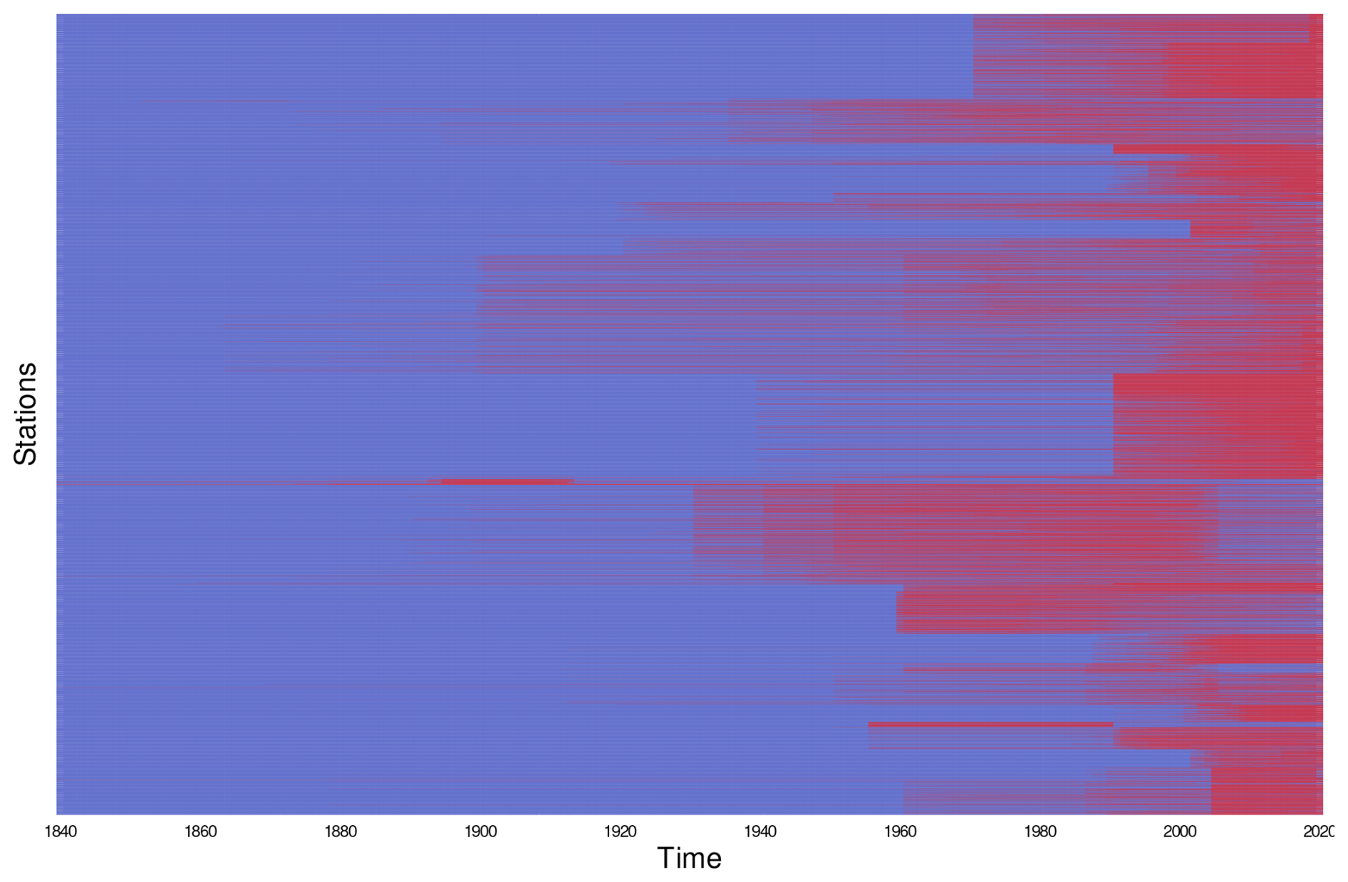
Figure A1 Heatmap showing the complex time structure of EEAR-Clim. The time extent of each station is highlighted using red shades, limited to the 1840–2020 period.

Table A1 Summary table of break detection results based on the multi-method comparison. The numbers and related percentages of homogeneous, inhomogeneous, and not tested time series are reported. Not tested time series are grouped into those with an extent below 30 years and without enough reference stations.

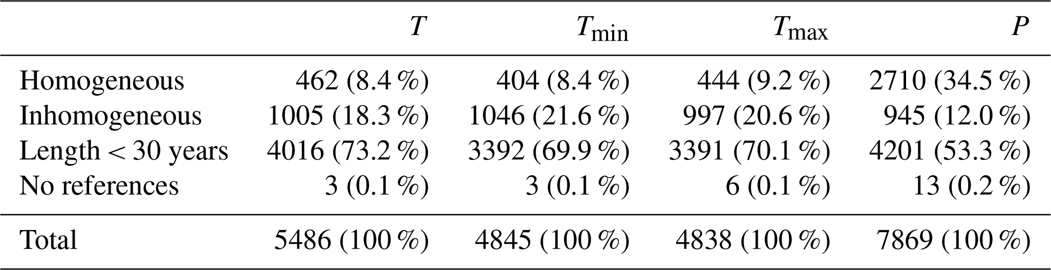
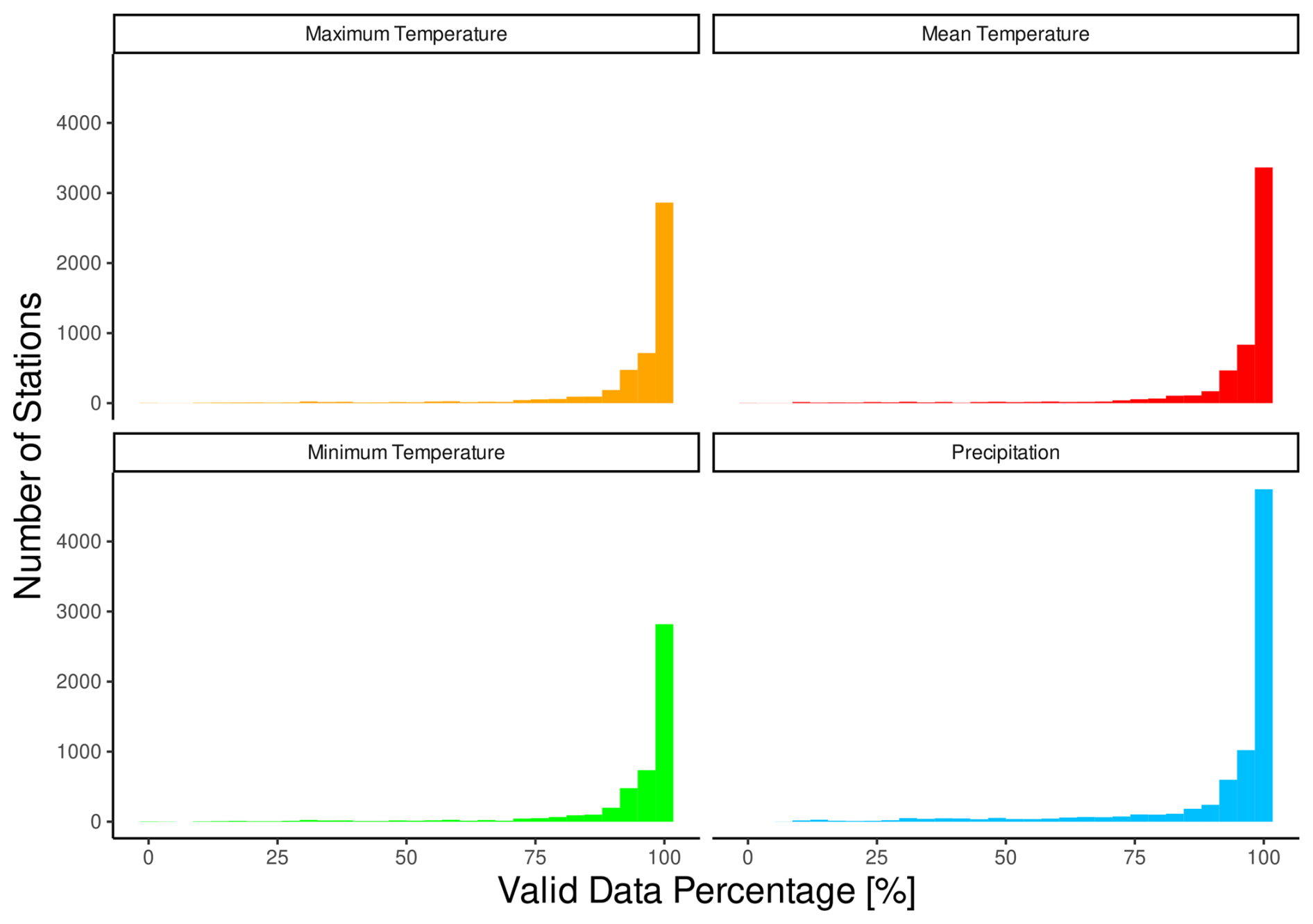
Figure A2 Distribution of time series over a valid data percentage for the mean, minimum, and maximum air temperature and for precipitation.

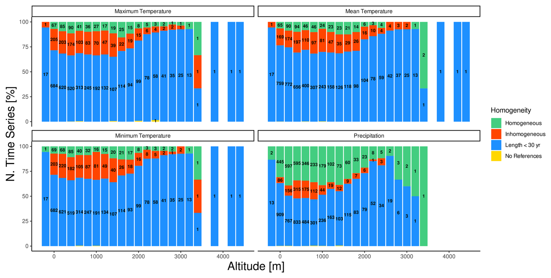
Figure A3 Distribution of homogeneous time series (green), inhomogeneous time series (red), insufficiently long time series (blue), and time series without references (yellow) over elevation for the mean, minimum, and maximum air temperature and for precipitation. The y axis indicates the percentage of stations in each category, while numbers within bars report the absolute numbers.

Appendix B: Correction of inhomogeneous precipitation data

The calculation of adjustments for precipitation time series affected by identified inhomogeneities follows the quantile-based procedure suggested by Squintu et al. (2019), but it is adapted for precipitation data. Daily values below 0.1 mm are not corrected to ensure consistency and avoid unrealistic results, such as negative precipitation amounts or dry days being converted into wet days. The computation of the adjustment factor $a_{i,j,q,m}$ (Eq. 2 in Squintu et al., 2019) and the final adjusted value $\stackrel{\mathrm{‾}}{v}$ (Eqs. 4 and 5 Squintu et al., 2019) have been modified accordingly. In particular, the adjustment factor $a_{i,j,q,m}$ is computed as follows:

$$\begin{array}{}\text{(B1)}& a_{i,j,q,m}={\displaystyle \frac{\frac{b_{q,m}}{r_{j,q,m}^{\mathrm{aft}}}}{\frac{s_{i,q,m}}{r_{j,q,m}^{\mathrm{bef}}}}}.\end{array}$$

Instead, the final adjustments are computed as the median over j values:

$$\begin{array}{}\text{(B2)}& \stackrel{\mathrm{̃}}{v_j}=v\cdot a_{\stackrel{\mathrm{̃}}{j,q,m}},\end{array}$$

thereby simply converting the temperature formula from additive to multiplicative and making it suitable for precipitation data.