Global greenhouse gas reconciliation 2022

In this study, we provide an update on the methodology and data used by Deng et al. (2022) to compare the national greenhouse gas inventories (NGHGIs) and atmospheric inversion model ensembles contributed by international research teams coordinated by the Global Carbon Project. The comparison framework uses transparent processing of the net ecosystem exchange fluxes of carbon dioxide (CO₂) from inversions to provide estimates of terrestrial carbon stock changes over managed land that can be used to evaluate NGHGIs. For methane (CH₄), and nitrous oxide (N₂O), we separate anthropogenic emissions from natural sources based directly on the inversion results to make them compatible with NGHGIs. Our global harmonized NGHGI database was updated with inventory data until February 2023 by compiling data from periodical United Nations Framework Convention on Climate Change (UNFCCC) inventories by Annex I countries and sporadic and less detailed emissions reports by non-Annex I countries given by national communications and biennial update reports. For the inversion data, we used an ensemble of 22 global inversions produced for the most recent assessments of the global budgets of CO₂, CH₄, and N₂O coordinated by the Global Carbon Project with ancillary data. The CO₂ inversion ensemble in this study goes through 2021, building on our previous report from 1990 to 2019, and includes three new satellite inversions compared to the previous study and an improved managed-land mask. As a result, although significant differences exist between the CO₂ inversion estimates, both satellite and in situ inversions over managed lands indicate that Russia and Canada had a larger land carbon sink in recent years than reported in their NGHGIs, while the NGHGIs reported a significant upward trend of carbon sink in Russia but a downward trend in Canada. For CH₄ and N₂O, the results of the new inversion ensembles are extended to 2020. Rapid increases in anthropogenic CH₄ emissions were observed in developing countries, with varying levels of agreement between NGHGIs and inversion results, while developed countries showed a slowly declining or stable trend in emissions. Much denser sampling of atmospheric CO₂ and CH₄ concentrations by different satellites, coordinated into a global constellation, is expected in the coming years. The methodology proposed here to compare inversion results with NGHGIs can be applied regularly for monitoring the effectiveness of mitigation policy and progress by countries to meet the objectives of their pledges. The dataset constructed for this study is publicly available at https://doi.org/10.5281/zenodo.13887128 (Deng et al., 2024).

1 Introduction

If modeled pathways align with nationally determined contributions (NDCs) declared prior to COP26 (in 2021) until 2030 and do not involve any subsequent increase in ambition, the projected global warming by 2100 would be 2.1–3.4 °C (IPCC, 2023). The global stocktake coordinated by the secretariat of the United Nations Framework Convention on Climate Change (UNFCCC) considers data from national greenhouse gas inventories (NGHGIs) to assess the collective climate progress toward curbing emissions. It is expected there will be differences in the quality of NGHGIs being reported to the UNFCCC (Perugini et al., 2021). UNFCCC Annex I parties, which include all OECD (Organisation for Economic Co-operation and Development) countries and several EITs (economies in transition), already report their emissions annually following the same IPCC guidelines (IPCC, 2006) in the Common Reporting Format, with a time latency of roughly 1.5 years. In contrast, non-Annex I parties, mostly developing and less developed countries, are currently not required to provide reports as regularly and in as detailed a format as Annex I parties and in a few cases use different IPCC guidelines in their national communications (NCs) or biennial update reports (BURs) submitted to the UNFCCC. Non-Annex I parties were scheduled in 2024 to move to regular and harmonized reporting of their emissions in the national inventory reports (NIRs) in the format of common reporting tables (CRTs), following the Paris Agreement's enhanced transparency framework (ETF).

The IPCC guidelines for NGHGIs encourage countries to use independent information to verify emissions and removals (IPCC, 1997, 2006, 2019), such as comparisons with independently compiled inventory databases (e.g., IEA, CDIAC, EDGAR, FAOSTAT) or with atmospheric mole fraction measurements interpreted by atmospheric inversion models (see Sect. 6.10.2 in IPCC, 2019). Such verification of “bottom-up” national reports against “top-down” atmospheric inversion results is not mandatory. However, a few countries (e.g., Switzerland, the United Kingdom, Aotearoa / New Zealand, and Australia) have already added inversions as a consistency check of their national reports. In our study, we utilized the latest global inversion results from the budget assessments of carbon dioxide (CO₂), methane (CH₄), and nitrous oxide (N₂O) conducted by the Global Carbon Project (GCP), focusing on three ensembles of inversions with global coverage. Compared to our previous study (Deng et al., 2022), the CO₂ inversion ensemble used in this study has been updated to the global CO₂ budget of Friedlingstein et al. (2022), which includes nine CO₂ inversions using mole fraction data from the surface network and/or retrieval products from the Greenhouse Gases Observing Satellite (GOSAT) and Orbiting Carbon Observatory-2 (OCO-2) satellites. The CH₄ inversion ensemble and N₂O inversion (Tian et al., 2024) ensemble used in this study are also extended to the 2020. As a result, the new ensembles cover up to 2021 for CO₂, 2020 for CH₄, and 2020 for N₂O, compared to 2019, 2017, and 2016, respectively, in our previous study (Deng et al., 2022), allowing us to track and analyze the most recent flux variations.

Our framework to process the inversion data aims at making them comparable to inventories at the scale of countries or groups of countries (i.e., with an area larger than the spatial resolution of atmospheric transport models typically used for inversions). Atmospheric inversions use a priori information for the spatial and temporal patterns of fluxes. Some inversions correct prior fluxes at the spatial resolution of their transport models to match atmospheric observations and use spatial error correlations (usually e-folding length scales) that tie the adjustment of fluxes from one grid cell to its neighbors at distances of tens to hundreds of kilometers. Other inversions adjust fluxes over coarse regions that are larger than the resolution of the transport model, implicitly assuming a perfect correlation of flux errors within these regions and causing an aggregation error (Kaminski et al., 2001). Thus, to minimize aggregation errors, the results of inversions are shown preferentially for selected countries that are large area emitters or large absorbers in the case of CO₂. We have selected a different set of countries or groups of countries for each gas, according to their importance in the global emission budget. According to the median of inversion data we used in this study, selected countries collectively represent ∼ 70 % of global fossil fuel CO₂ emissions, ∼ 90 % of global land CO₂ sink, ∼ 60 % of anthropogenic CH₄ emissions, and ∼ 55 % of anthropogenic N₂O emissions (Fig. S1 in the Supplement). To more robustly interpret global inversion results for comparison with inventories, we follow the same criterion and choose high-emitting countries covered (if possible) by atmospheric measurements, although most selected tropical countries have few or no atmospheric in situ stations. Uncertainties are given by the spread among inversion models (min–max range given the small number of inversions), and the causes for discrepancies with inventories are analyzed systematically and on a case-by-case basis, considering both individual countries and specific greenhouse gases, for annual variations and for mean budgets over several years.

Based on the newly updated inversion results and inventory and on an improvement in the methodology framework proposed in the previous study (Deng et al., 2022), we specifically address the following questions: (1) how do inversion models compare with NGHGIs for the three gases? (2) What are the plausible reasons for mismatches between inversions and NGHGIs? (3) Did the new maps of managed-land masks in this study reduce the mismatch between the inversions and NGHGIs for CO₂ and N₂O? (4) What independent information can be extracted from inversions to evaluate the mean values or the trends of greenhouse gas emissions and removals? (5) Does this information exhibit good agreement with NGHGIs? And (6) how do satellite-retrieval-driven inversion models differ from the surface in situ and flask-sampling-driven inversion model results?

Section 2 presents the updated global database of national emissions reports for selected countries and its grouping into sectors, the global atmospheric inversions used for the study, and the processing of fluxes from these inversions to make their results as comparable as possible with inventories. The time series of inversions compared with inventories for each gas, with insights into key sectors for CH₄, are discussed in Sects. 3 to 5. The Discussion section (Sect. 6) focuses on the plausible reasons for mismatches between inversions and NGHGIs, comparison between inversion ensembles in this study and the previous study, and the different priors applied in the CH₄ inversions. Finally, concluding remarks are drawn on how inversions could be used systematically to support the evaluation and possible improvement of inventories to reach the goals of the Paris Agreement.

2 Material and methods

2.1 Compilation and harmonization of national inventories reported to the UNFCCC

All UNFCCC parties shall periodically update and submit their national GHG inventories of emissions by sources and removals by sinks to the convention parties. Annex I countries submit their NIRs in Common Reporting Format (CRF) tables every year with a complete time series starting in 1990. Non-Annex I parties are required to submit their NCs roughly every 4 years after entering the convention and have submitted BURs every 2 years since 2014. Currently, there are in total 427 submissions of NCs and over 166 submissions of BURs (UNFCCC, 2021b, a) (Fig. 1).

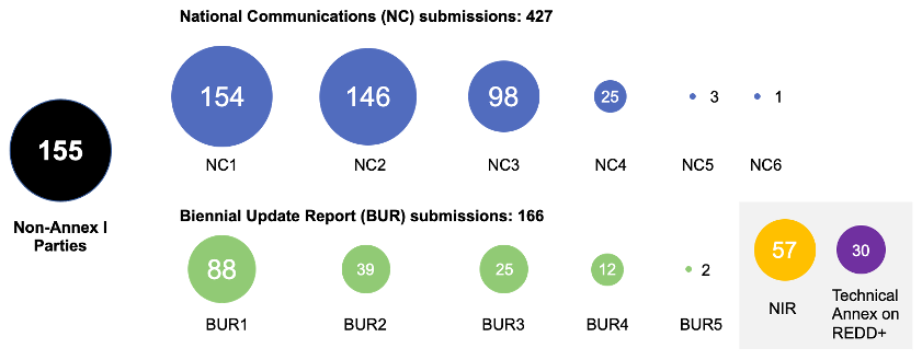
Figure 1 Numbers of non-Annex I parties for each submission round (as of 28 February 2023). The numbers in the middle of the dots denote the numbers of non-Annex I parties for each submission, the black dot denotes the total number of non-Annex I parties, the blue dots denote the numbers of non-Annex I parties who have submitted national communications (NCs), the green dots denote the numbers of biennial update reports (BURs), the yellow dot denotes the number of national inventory reports (NIR), and the purple dot denotes the number of technical annexes on REDD+. The numbers after the NC and BUR headings denote the total number of submission reports.

We collected NGHGI data submitted to the UNFCCC by 28 February 2023. For Annex I countries, data collection is straightforward, as their reports are provided as Excel files under the Common Reporting Format (CRF) until the year 2020, last accessed on 28 February 2023. For non-Annex I countries, the data were directly extracted from the original reports provided in portable document format (PDF), last accessed on 28 February 2023. Data from successive reports for the same country were extracted, except when they relate to the same years, in which case only the latest version is considered. While Annex I countries are required to compile their inventory following 2006 IPCC guidelines and the subdivision between sectors established by the UNFCCC decision (dec. 24/CP.19), non-Annex I countries are increasingly adopting the 2006 IPCC guidelines, although some still utilize the older 1996 IPCC guidelines, with different approaches and sectors. Consequently, the methods used and the reported sectors may differ among NCs and BURs.

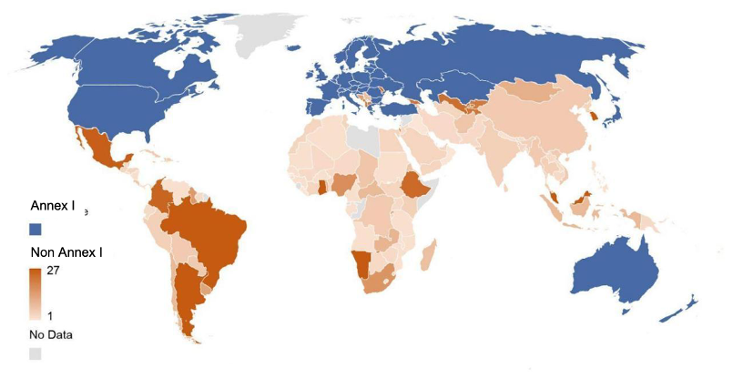
Figure 2 Number of years covered by NGHGI reports (NC+BUR) in each non-Annex I country (as of 28 February 2023). Emissions from Greenland are reported by Denmark.

2.2 Atmospheric inversions

2.2.1 CO₂ inversions

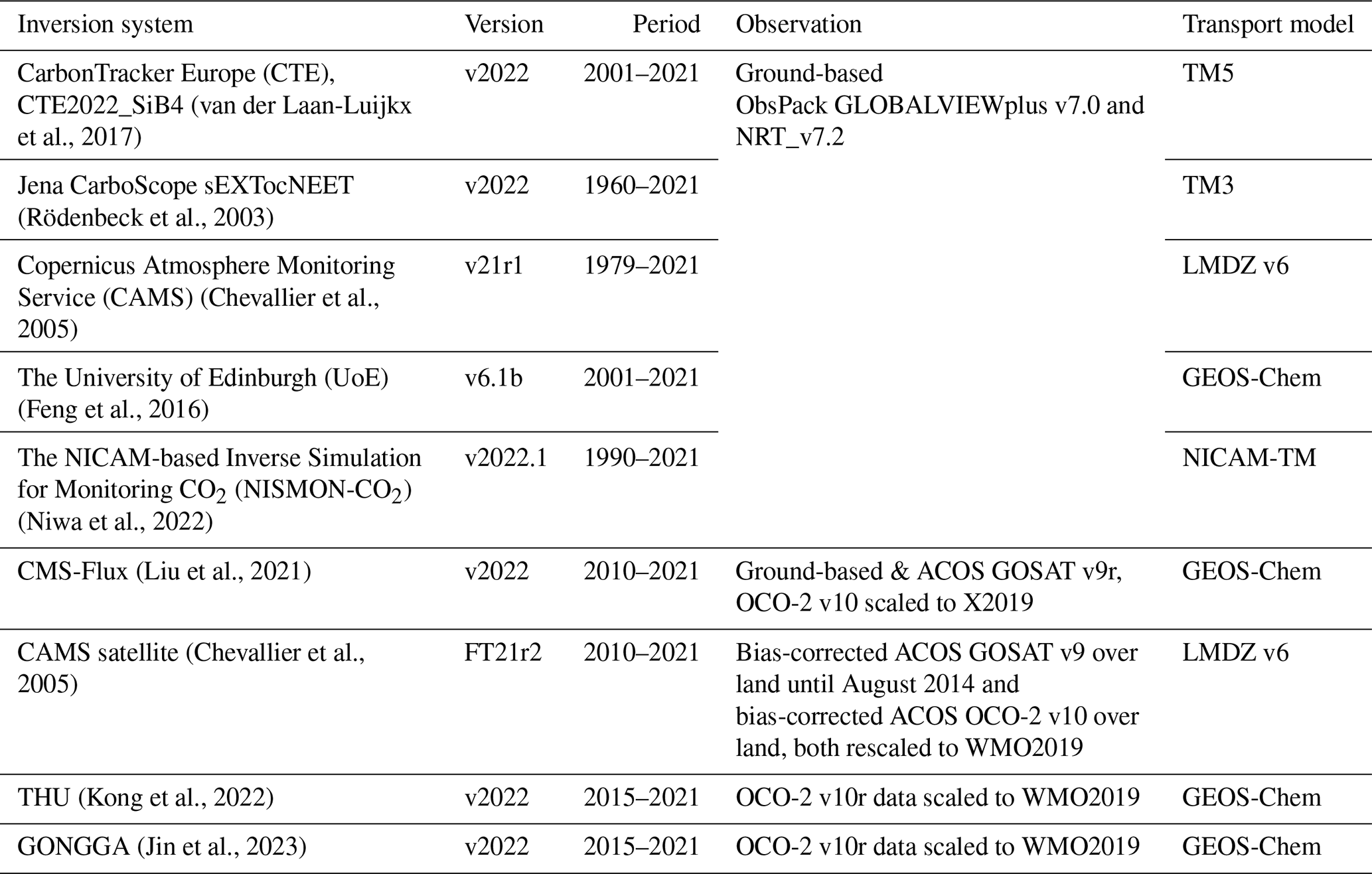
Nine CO₂ inversion systems from the Global Carbon Budget 2022 of the GCP (Friedlingstein et al., 2022) are used (Table 1), comprising CarbonTracker Europe (CTE) v2022 (van der Laan-Luijkx et al., 2017), Jena CarboScope v2022 (Rödenbeck et al., 2003), the surface air-sample inversion from the Copernicus Atmosphere Monitoring Service (CAMS) v21r1 (Chevallier et al., 2005), the inversion from the CAMS satellite FT21r2 (Chevallier et al., 2005), the inversion from the University of Edinburgh (UoE) v6.1b (Feng et al., 2016), the NICAM-based Inverse Simulation for Monitoring CO₂ (NISMON-CO₂) v2022.1 (Niwa et al., 2022), CMS-Flux v2022 (Liu et al., 2021), GONGGA v2022 (Jin et al., 2023), and THU v2022 (Kong et al., 2022). A variety of transport models are used by these systems, which allows for representing a major driver factor behind differences in flux estimates based on atmospheric inversions, particularly their distribution over latitudinal bands. Among the nine inversions, four systems (CAMS satellite FT21r2, GONGGA v2022, THU v2022, and CMS-Flux v2022) utilize satellite CO₂ column retrievals from GOSAT and/or OCO-2, calibrated to the World Meteorological Organization (WMO) 2019 standards. CMS-Flux additionally incorporates in situ-observed CO₂ mole fraction records. The remaining five inversion systems (CAMS v21r1, CTE v2022, Jena CarboScope v2022, UoE v6.1b, and NISMON-CO₂ v2022.1) solely rely on CO₂ mole fractions that were observed in situ or collected in flasks (Schuldt et al., 2021, 2022). The CO₂ inversion records extend up to and include 2021. Their flux estimates are available at https://meta.icos-cp.eu/objects/GahdRITjT22GGmq_GCi4o_wy (last access: 10 February 2024), and details are summarized in Table 1.

Table 1 Atmospheric CO₂ inversions used in this study (Friedlingstein et al., 2022).

2.2.2 CH₄ inversions

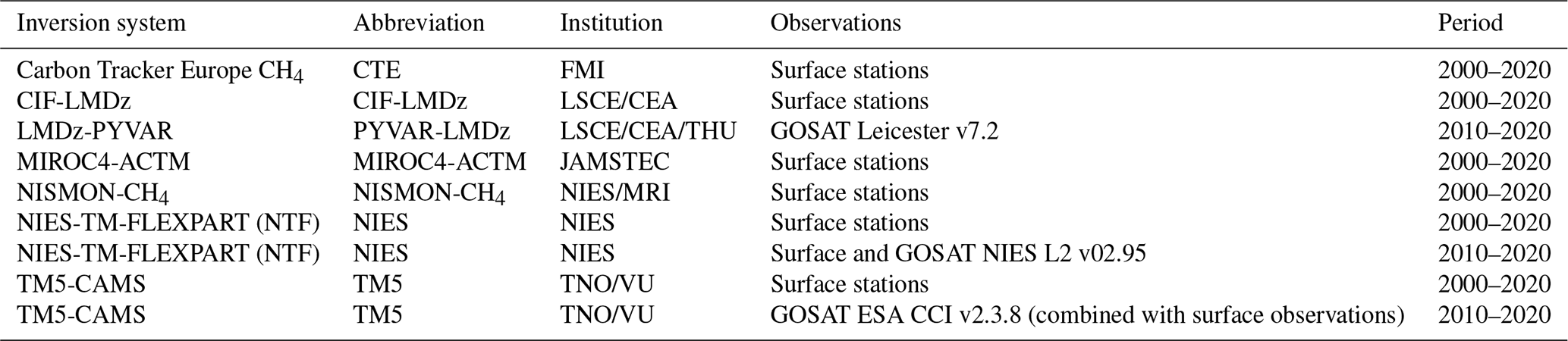
The CH₄ emissions come from the new ensemble of inversions (Saunois et al., 2024) from 2000 to 2020, using seven different inverse systems for a total of nine inversions (Table 2). The inverse systems include CarbonTracker Europe CH₄ (Tsuruta et al., 2017), LMDZ-PYVAR (Yin et al., 2015; Zheng et al., 2018), CIF-LMDZ (Berchet et al., 2021), MIROC4-ACTM (Patra et al., 2018; Chandra et al., 2021), NISMON-CH₄ (Niwa et al., 2022), NIES-TM-FLEXPART (Maksyutov et al., 2021; Janardanan et al., 2024), and TM5-CAMS (Segers and Houweling, 2017). This ensemble of inversions gathers various chemistry transport models, differing in vertical and horizontal resolutions, meteorological forcing, advection (horizontal transport of air) and convection (vertical transport) schemes, and boundary layer mixing (detailed characteristics can be found in Table S11 in Saunois et al., 2024). Including these different systems is a conservative approach that allows us to cover different potential uncertainties in the inversion, among them model transport, setup issues, and prior dependency. All inversions except two use updated common prior emission maps for natural and anthropogenic prior emissions divided into 12 sectors, particularly the EDGAR v6.0 inventory for prior fossil fuel emissions (Crippa et al., 2021, extrapolated to 1 January 2021) and GFED for fires and ecosystem models for wetland emissions. During the production of the inversion simulations, the GAINS inventory (Höglund-Isaksson, 2020) was proposed to use another prior for fossil fuel sources, instead of using EDGAR v6 (see Supplementary Text 3 in Saunois et al., 2024). GAINS has higher fossil emissions, in particular over the USA, and a higher increase in fossil emissions over time in the USA (Tibrewal et al., 2024). As Tibrewal et al. (2024) showed that inversions are strongly attracted to their priors, comparison between results with GAINS and EDGAR v6 priors is informative about how robust inversions are to their priors when they are used to “verify” NGHGIs. Some inversions optimize emissions in groups of sectors, and others only provide total gridded emissions (MIROC4-ACTM and TM5-CAMS; details can be found in Table S10 in Saunois et al., 2024). For the latter, we computed the emission from each sector within each pixel based on the proportion of the prior fluxes. Such processing can lead to significant uncertainties if not all sources increase or change at the same rate in a given region/pixel. The inversions assimilating surface stations mole fraction observations provide results since 2000, and those assimilating satellite observations from column CH₄ measurements (XCH₄) of GOSAT provide results since 2010, the first full year of GOSAT observations. Inversion results were gridded into 1° by 1° monthly emission maps and aggregated nationally using a country mask (Klein Goldewijk et al., 2017).

Table 2 Atmospheric CH₄ inversions used in this study (Saunois et al., 2024).

2.2.3 N₂O inversions

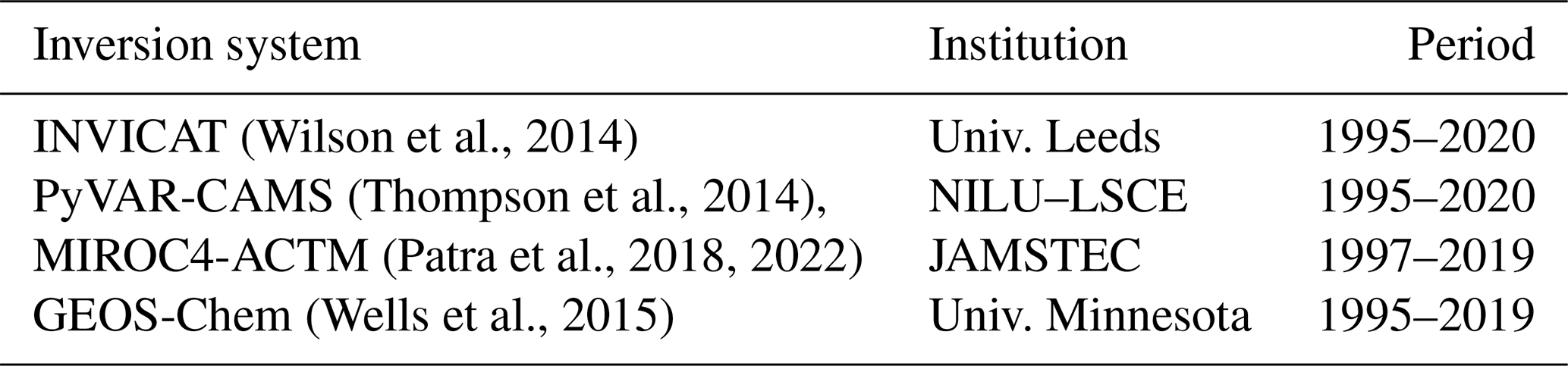
Four N₂O inversion systems from the updated GCP Global Nitrous Oxide Budget (Tian et al., 2024) are used (Table 3): INVICAT (Wilson et al., 2014), PyVAR-CAMS (Thompson et al., 2014), MIROC4-ACTM (Patra et al., 2018, 2022), and GEOS-Chem (Wells et al., 2015). The N₂O inversion results are updated up to 2020.

Table 3 Atmospheric N₂O inversions used in this study (Tian et al., 2024).

2.2.4 Aggregating the gridded inversion results into national totals

To obtain national annual-scale flux estimates, we aggregated the gridded flux maps of each inversion with various native resolutions following the methodology outlined in Chevallier (2021). This involved using the 0.08° × 0.08° land country mask of Klein Goldewijk et al. (2017) to calculate the fraction of each country in each inversion grid box.

2.3 Processing of CO₂ inversion data for comparison with NGHGIs

2.3.1 Fossil fuel emissions re-gridding – managed-land mask

To analyze terrestrial CO₂ fluxes, we subtracted the same fossil fuel emissions (including cement) of GridFEDv2022.2 (Jones et al., 2022) from the total CO₂ flux of each inversion. This is equivalent to assuming perfect knowledge of fossil emissions, adding up to a global total of 9.7 Gt C yr⁻¹ for the year 2021. The dataset used national annual emission estimates from the Global Carbon Budget 2022 (Friedlingstein et al., 2022), which uses the reported NGHGI data from Annex I countries that are assumed to be broadly consistent with the non-Annex I countries. This assumption may lead to underestimating the uncertainty in terrestrial CO₂ fluxes deduced from inversions.

As defined in the IPCC guidelines for NGHGIs (IPCC, 2006), only CO₂ emissions and removals from managed land are reported in NGHGIs as a proxy for human-induced effects (direct effects and indirect effects such as CO₂ fertilization and nitrogen deposition). However, inversion models retrieve all CO₂ fluxes (due to both direct and indirect effects, as well as the natural interannual variability) over all land types. We thus retained inversions' national estimates of the net ecosystem exchange (NEE) CO₂ flux ($F_{\mathrm{ML}}^{\text{inv NEE}}$) over managed-land grid cells only (ML here defined as all land except intact forests) because the fluxes over unmanaged land are not counted by NGHGIs. We use NEE from the definition of Ciais et al. (2021), representing all non-fossil CO₂ exchange fluxes between terrestrial surfaces and the atmosphere. Other work may use net biome production (NBP) with a similar meaning. CO₂ fluxes over unmanaged lands were excluded from the terrestrial CO₂ flux totals that will be compared with NGHGIs, proportional to their presence in each inversion grid box. The new maps of non-intact forests are compiled by Grassi et al. (2023). These maps include official country-managed forest and other managed-land areas for Canada and Brazil used for their NGHGIs and the intact forest map (Potapov et al., 2017) as a substitute for unmanaged land where country-based information is not available. For Russia, we used non-intact forest maps for each province, with thresholds adjusted to match the official managed-land areas from Russia's NIRs and assumed that all grasslands were managed. This approach assumes that non-intact forest areas can serve as a reasonably good proxy for managed forests reported in the NGHGIs (Grassi et al., 2021, 2023). It is important to note that this approach is somewhat arbitrary, as highlighted in previous studies (Ogle et al., 2018; Chevallier, 2021; Grassi et al., 2021). However, in the absence of a machine-readable definition of managed plots in many NGHGIs, there is currently no better alternative available.

2.3.2 Adjusting CO₂ fluxes due to lateral carbon transport by crop and wood product trade and by rivers

In addition to the extraction of fossil CO₂ flux and managed-land CO₂ flux, there are CO₂ fluxes that are part of $F_{\mathrm{ML}}^{\text{inv NEE}}$ but are not counted by NGHGIs. These fluxes are induced by (i) soil to river to ocean carbon export ($F_{\mathrm{ML}}^{\mathrm{rivers}}$), which has an anthropogenic and a natural component (Regnier et al., 2013), and (ii) net anthropogenic export of crop and wood products across each country's boundary ($F_{\mathrm{ant}}^{\text{crop trade}}$ and $F_{\mathrm{ant}}^{\text{wood trade}}$). The magnitudes of these CO₂ fluxes are different between countries, and values from the selected countries are presented in Fig. S2. We assume that NGHGIs include CO₂ losses from fire (wildfire and prescribed fire) and other disturbances (wind, pests) and from domestic harvesting, as recommended by the IPCC reporting guidelines (IPCC, 2006, 2019) (although some countries, such as Canada and Australia exclude some emissions from these disturbances, and the subsequent removals from the same areas; Grassi et al., 2023). The adjusted inversion NEE that can be compared with inventories, $F_{\mathrm{adj}}^{\text{inv NEE}}$, is given by

$$\begin{array}{}\text{(1)}& \begin{array}{rl}{F}_{\mathrm{adj}}^{\text{inv NEE}}& =F_{\mathrm{ML}}^{\text{inv NEE}}-F_{\mathrm{ML}}^{\mathrm{rivers}}-F_{\mathrm{ant}}^{\text{crop trade}}-\\ & F_{\mathrm{ant}}^{\text{wood trade}}\iff F_{\text{ant-nf}}^{\mathrm{ni}},\end{array}\end{array}$$

where the sign ⇔ means “compared with”, $F_{\text{ant-nf}}^{\mathrm{ni}}$ is the non-fossil part of the anthropogenic CO₂ flux from NGHGIs, $F_{\mathrm{ML}}^{\text{rivers}}$ is the sum of the natural and anthropogenic CO₂ flux on land from CO₂ fixation by plants that is leached as carbon via soils and channeled to inland waters to be exported to the ocean or to another country. All countries export river carbon, but some countries also receive river inputs; e.g., Romania receives carbon from Serbia via the Danube River. We estimated the lateral carbon export by rivers minus the imports from rivers entering each country, including dissolved organic carbon, particulate organic carbon, and dissolved inorganic carbon of atmospheric origin distinguished from lithogenic origin, using the data and methodology described by Ciais et al. (2021). Data are from Mayorga et al. (2010) and Hartmann et al. (2009) and follow the approach of Ciais et al. (2021) proposed for large regions. We also extracted the lateral flux by rivers over the managed land using the same methodology as for inversion CO₂ flux. Thus, in a country that only exports river carbon to the ocean, the amount of carbon exported is equivalent to an atmospheric CO₂ sink, denoted as $F_{\mathrm{ML}}^{\mathrm{rivers}}$ as in Eq. (1), thus ignoring burial, which is a small term. Over a country that receives carbon from rivers flowing into its territory, a small national CO₂ outgassing is produced by a fraction of this imported flux. In that case, we assumed that the fraction of outgassed to incoming river carbon is equal to the fraction of outgassed to soil-leached carbon in the RECCAP2 region to which a country belongs, estimated with data from Ciais et al. (2021).

$F_{\mathrm{ant}}^{\text{crop trade}}$ is the sum of CO₂ sinks and sources induced by the trade of crop products. This flux was estimated from the annual trade balance of crop commodities calculated for each country from data from the United Nations Statistics Division of the Food and Agriculture Organization (FAOSTAT) combined with the carbon content values of each commodity (Xu et al., 2021; FAO, 2024). All the traded carbon in crop commodities is assumed to be oxidized as CO₂ in 1 year, neglecting stock changes of products and the fraction of carbon from crop products going to waste pools and sewage waters after consumption and thus not necessarily oxidized into atmospheric CO₂. $F_{\mathrm{ant}}^{\text{wood trade}}$ is the sum of CO₂ sinks and sources induced by the trade of wood products (Zscheischler et al., 2017). Here, we followed Ciais et al. (2021), who used a bookkeeping model to calculate the fraction of domestically produced and imported carbon in wood products that are oxidized in each country during subsequent years, with product lifetimes defined by Mason Earles et al. (2012) and encompassing all products (including roundwood and processed products). The underlying assumption in estimating CO₂ fluxes from wood harvest is that the emissions from domestically harvested wood, in addition to those from imported wood minus those from exported wood that are not allocated to wood product pools, are released into the atmosphere during the year of harvest. Conversely, emissions from wood allocated to wood product pools are gradually released into the atmosphere over time, based on their respective lifetimes. Domestic harvest is assumed to be balanced by an atmospheric CO₂ sink of equivalent magnitude, which is not necessarily the case given that harvest is rarely in equilibrium with forest increment, but inversion NEE will correct for this imbalance in our results, and thus harvest can be compared with NGHGIs. We included in the $F_{\mathrm{ant}}^{\text{crop trade}}$ flux the emissions of CO₂ by domestic animals consuming specific crop products delivered as feed. On the other hand, emissions of CO₂ from grazing animals and the decomposition of their manure are supposed to occur in the same grid box where grass is grazed so that the CO₂ net flux captured by an inversion is comparable with grazed grasslands' carbon stock changes of inventories. Emissions of reduced carbon compounds (VOCs, CH₄, CO) are not included in this analysis (see Ciais et al., 2021, for a discussion of their importance in inversion CO₂ budgets).

In summary, the purpose of the adjustment of Eq. (1) is to make inversion output comparable to the NGHGIs that do not include $F_{\mathrm{ML}}^{\mathrm{rivers}}$, $F_{\mathrm{ant}}^{\text{crop trade}}$, and $F_{\mathrm{ant}}^{\text{wood trade}}$. The UNFCCC accounting rules (IPCC, 2006) assume that all the harvested wood products are emitted in the territory of a country that produces them, which is equivalent to ignoring $F_{\mathrm{ant}}^{\text{wood trade}}$ as a national sink or source of CO₂, hence the need to remove $F_{\mathrm{ant}}^{\text{wood trade}}$ from inversion NEE. The adjusted inversion fluxes from Eq. (1) depict the national CO₂ stock change which better match the carbon accounting system boundaries of UNFCCC NGHGIs. In the following, we will only discuss adjusted inversion CO₂ fluxes ($F_{\mathrm{adj}}^{\text{inv NEE}}$), but for simplicity we call them “inversion fluxes”.

2.4 Processing of CH₄ inversions for comparison with national inventories

Most atmospheric inversions derive total net CH₄ emissions at the surface as it is difficult for them to disentangle overlapping emissions from different sectors at the pixel/regional scale based on atmospheric CH₄ observations only. However, five of the seven inverse systems solve for some source categories owing to different spatio-temporal distributions between the sectors. For each inversion, monthly gridded posterior flux estimates were provided at 1° × 1° grid resolution for the net flux at the surface ($E_{\mathrm{net}}^{\mathrm{inv}}$); the soil uptake at the surface ($E_{\mathrm{soil}}^{\mathrm{inv}}$); the total emission at the surface ($E_{\mathrm{tot}}^{\mathrm{inv}}$); and five emitting “super sectors” which regroup several IPCC sectors – agriculture and waste ($E_{\mathrm{AgW}}^{\mathrm{inv}}$), fossil fuel ($E_{\mathrm{FF}}^{\mathrm{inv}}$), biomass and biofuel burning ($E_{\mathrm{BB}}^{\mathrm{inv}}$), wetlands ($E_{\mathrm{Wet}}^{\mathrm{inv}}$), and other natural ($E_{\mathrm{Oth}}^{\mathrm{inv}}$) emissions. Considering the soil uptake to be a “negative source” given separately, the following equation applies:

$$\begin{array}{}\text{(2)}& \begin{array}{rl}{E}_{\mathrm{net}}^{\mathrm{inv}}& =E_{\mathrm{tot}}^{\mathrm{inv}}+E_{\mathrm{soil}}^{\mathrm{inv}}=E_{\mathrm{AgW}}^{\mathrm{inv}}+E_{\mathrm{FF}}^{\mathrm{inv}}\\ & +E_{\mathrm{BB}}^{\mathrm{inv}}+E_{\mathrm{Wet}}^{\mathrm{inv}}+E_{\mathrm{Oth}}^{\mathrm{inv}}+E_{\mathrm{soil}}^{\mathrm{inv}}.\end{array}\end{array}$$

For inversions solving for net emissions only, the partitioning into source sectors was created based on using a fixed ratio of sources calculated from prior flux information at the pixel scale. For inversions solving for some categories, a similar approach was used to partition the solved categories into the five aforementioned emitting sectors. Such processing can lead to significant uncertainties if not all sources increase or change at the same rate in a given region/pixel. National values have been estimated using the country land mask described in the CO₂ section (Sect. 2.3.1); thus offshore emissions are not counted as part of inversion results unless they are in a coastal grid cell.

In our previous study (Deng et al., 2022), four methods were proposed to separate CH₄ anthropogenic emissions from inversions $(E_{\mathrm{Anth}}^{\mathrm{inv}}$) and compare them with national inventories ($E_{\mathrm{Anth}}^{\mathrm{ni}}$), aiming to discuss the uncertainties in anthropogenic CH₄ emissions associated with the chosen separation methods. These four methods comprise (1) summing prior estimates based on inversions for anthropogenic sectors (method 1), (2) subtracting natural emissions from total fluxes (method 2), and (3) subtracting natural emissions derived from other bottom-up assessments from the total inversion flux (methods 3.1 and 3.2, differing only in the bottom-up wetland CH₄ data used). The calculations of anthropogenic emissions by each method were performed separately for GOSAT inversions and in situ inversions. However, the uncertainty from the separation method is generally much smaller than the variability between different inversion models (see Fig. 9 in Deng et al., 2022). Therefore, we apply only one method in this study, which consists of using inversion partitioning as defined in Saunois et al. (2020):

$$\begin{array}{}\text{(3)}& E_{\mathrm{Anth}}^{\mathrm{inv}}=E_{\mathrm{AgW}}^{\mathrm{inv}}+E_{\mathrm{FF}}^{\mathrm{inv}}+E_{\mathrm{BB}}^{\mathrm{inv}}-E_{\mathrm{wildfires}}^{\mathrm{BU}}\iff E_{\mathrm{Anth}}^{\mathrm{ni}}.\end{array}$$

This method has some uncertainties. First, the partitioning relies on prior fractions within each pixel, and second, emissions from wildfires are counted for in the biomass and biofuel burning (BB) inversion category, while they are not necessarily reported in NGHGIs. The BB inversion category includes methane emissions from wildfires in forests, savannahs, grasslands, peats, agricultural residues, and the burning of biofuels in the residential sector (stoves, boilers, fireplaces). Therefore, we subtracted bottom-up (BU) emissions from wildfires ($E_{\mathrm{wildfires}}^{\mathrm{BU}}$) based on the GFEDv4 dataset (van Wees et al., 2022) using its reported dry matter burned and CH₄ emission factors. Because the GFEDv4 dataset also reports specific agricultural and waste fire emissions data, we assumed that those fires (on managed lands) are reported by NGHGIs, so they were not counted in $E_{\mathrm{wildfires}}^{\mathrm{BU}}$. Figure S3 presents a comparison between our adjusted BB flux and the wood fuel emissions reported by Flammini et al. (2023). This comparison highlights the broader scope and definition of our adjusted BB flux, illustrating the differences in emissions estimation methodologies.

2.5 Processing of N₂O inversions for comparison with inventories

We subtracted estimates of natural N₂O sources from the N₂O emission budget ($E_{\mathrm{tot}}^{\mathrm{inv}}$) of each inversion to provide inversions of anthropogenic emissions ($E_{\mathrm{ant}}^{\mathrm{inv}}$) that can be compared with national inventories ($E_{\mathrm{ant}}^{\mathrm{ni}}$):

$$\begin{array}{}\text{(4)}& E_{\mathrm{ant}}^{\mathrm{inv}}=E_{\mathrm{ML}}^{\mathrm{inv}}-E_{\mathrm{nat}}^{\mathrm{aq}}-E_{\mathrm{wildfires}}^{\mathrm{GFED}}\iff E_{\mathrm{ant}}^{\mathrm{ni}}.\end{array}$$

Here, the natural N₂O sources include natural emissions from freshwater systems (${}_{\mathrm{nat}}^{\mathrm{aq}}$) and natural emissions from wildfires (${}_{\mathrm{ant}}^{\mathrm{ni}}$).

In our previous study, intact forest grid cells (assumed unmanaged) from Potapov et al. (2017) and lightly grazed grassland areas from Chang et al. (2021) were removed from the gridded N₂O emissions in proportion to their presence in each inversion grid box. Here we used the new managed-land mask defined in Sect. 2.3 to filter gridded N₂O emissions from inversions to obtain $E_{\mathrm{ML}}^{\mathrm{inv}}$. We verified that the inversion grid box fractions classified as unmanaged do not contain point source emissions from the industry and energy and from diffuse emissions from the waste sector to make sure that we do not inadvertently remove anthropogenic sources by masking unmanaged pixels. From the EDGAR v4.3.2 inventory (Janssens-Maenhout et al., 2019), we found that N₂O from wastewater handling covers a relatively large area that might be partly located in unmanaged land. But the corresponding emission rates are more than 1 order of magnitude smaller than those from agricultural soils. For other sectors, only very few of the unmanaged grid boxes contain point sources, and none of them have an emission rate that is comparable with agricultural soils (managed land). Thus, our assumption that emissions from these other anthropogenic sectors are primarily over managed-land pixels is solid (other sectors include the power industry; oil refineries and transformation industry; combustion for manufacturing; aviation; road transportation, no resuspension; railways, pipelines, off-road transport; shipping; energy for buildings; chemical processes; solvents and product use; solid waste incineration; wastewater handling; and solid waste landfills).

The flux $E_{\mathrm{nat}}^{\mathrm{aq}}$ is the natural emission from freshwater systems given by a gridded simulation of the DLEM (Yao et al., 2019) describing pre-industrial N₂O emissions from N leached by soils and lost to the atmosphere by rivers in the absence of anthropogenic perturbations (considered the average of 1900–1910). Natural emissions from lakes were estimated only at a global scale by Tian et al. (2020) and represent a small fraction of rivers' emissions. Therefore, they are neglected in this study. The flux $E_{\mathrm{wildfires}}^{\mathrm{GFED}}$ is based on the GFED4s dataset (van Wees et al., 2022) using its reported dry matter burned and N₂O emission factors. Because the GFED dataset reports specific agricultural and waste fire emissions data, we assume that those fires (on managed lands) are reported by NGHGIs, so they were not counted in $E_{\mathrm{wildfires}}^{\mathrm{GFED}}$, just like for CH₄ emissions. Note that there could also be a background natural N₂O emission from natural soils over managed lands ($E_{\text{ML}}^{\mathrm{soil}}$) which is not necessarily reported by NGHGIs. We did not try to subtract this flux from managed-land emissions because we assumed that, after a land-use change from natural to fertilized agricultural land, background emissions decrease and become very small compared to N-fertilizer-induced anthropogenic emissions. In a future study, we could use for $E_{\text{ML}}^{\mathrm{soil}}$ the estimate given by simulations of pre-industrial N₂O emissions from the NMIP ensemble of dynamic vegetation models with carbon–nitrogen interactions (number of models n=7), namely, their simulation S0, in which climate forcing is recycled from 1901–1920, CO₂ is at the level of 1860, and no anthropogenic nitrogen is added to terrestrial ecosystems (Tian et al., 2019).

Another important point to ensure a rigorous comparison between inversion and NGHGI data is whether anthropogenic indirect emissions (AIEs) of N₂O are reported in NGHGI reports. This is not always the case even though UNFCCC parties are required to report these in their NGHGIs according to the IPCC guidelines. For example, South Africa's BUR3 did not report indirect N₂O emissions due to the lack of activity data. AIEs arise from anthropogenic nitrogen from fertilizers leached to rivers and anthropogenic nitrogen deposited from the atmosphere to soils. AIEs typically represent 20 % of direct anthropogenic emissions and cannot be ignored in a comparison with inversions. For Annex I countries, AIEs are systematically reported, generally based on emission factors since these fluxes cannot be directly measured, and we assumed that indirect emissions only occur on managed land. For non-Annex I countries, we checked manually from the original NC and BUR documents if AIE was reported or not by each non-Annex I country. If AIEs were reported by a country, they were used as such to compare NGHGI data with inversion results and were grouped into the agricultural sector. If they were not reported or if their values were outside plausible ranges, AIEs were independently estimated by the perturbation simulation of N fertilizer leaching, CO₂, and climate applied to river and lake fluxes in the DLEM model (Yao et al., 2019) and by the perturbation simulation of atmospheric nitrogen deposition on N₂O fluxes from the NMIP model ensemble (Tian et al., 2019).

2.6 Grouping sectors for comparison

The bottom-up NGHGIs are compiled based on activity data (statistics) following the 1996/2006 IPCC guidelines (IPCC, 1997, 2006), with detailed information on subsectors. However, the top-down inversions can only distinguish between very few groups of sectors at most. Thus, in this study, we aggregated NGHGI sectors into some super sectors to make inversions and inventories comparable for each GHG (Table 4). For CO₂, the inversions are divided into two aggregated super sectors: (1) fossil fuel and cement CO₂ emissions and (2) adjusted net land flux. Inversions use a prior gridded fossil fuel dataset as summarized in Sect. 2.3.1; thus, in this study, we compare only the net land flux between inversions and inventories. To calculate the net land flux over managed lands from NGHGIs, we subtracted fossil emissions from the IPCC CRF (1) “energy” and (2) “industrial processes” (or (2) “industrial processes and product use”) sectors from the “total GHG emissions including LULUCF/LUCF” (or “total national emissions and removals”) sector. For CH₄, we compare inversions and inventories based on three super sectors, comprising “fossil”, “agriculture and waste”, and “total anthropogenic”. To compare with NGHGIs, we group the IPCC CRF sectors of (1) “energy” and (2) “industrial processes” (or (2) “industrial processes and product use”), excluding biofuel burning (reported under the (1) energy sector), into the super sector of fossil; we group sectors of (4) “agriculture” (or (3) “agriculture”) and (6) “waste” (or (5) “waste”) into the super sector of agriculture and waste; and we aggregate anthropogenic flux from “fossil”, “agriculture and waste”, and “biofuel burning” into anthropogenic. For N₂O, we group the NGHGI sectors into anthropogenic flux, being the sum of (1) energy + (2) industrial processes (or (2) industrial processes and product use) + (4) agriculture (or (3) agriculture) + (6) waste (or (5) waste) + anthropogenic indirect emissions.

Table 4 Grouping of NGHGI sectors into aggregated super sectors for comparisons with inversions.

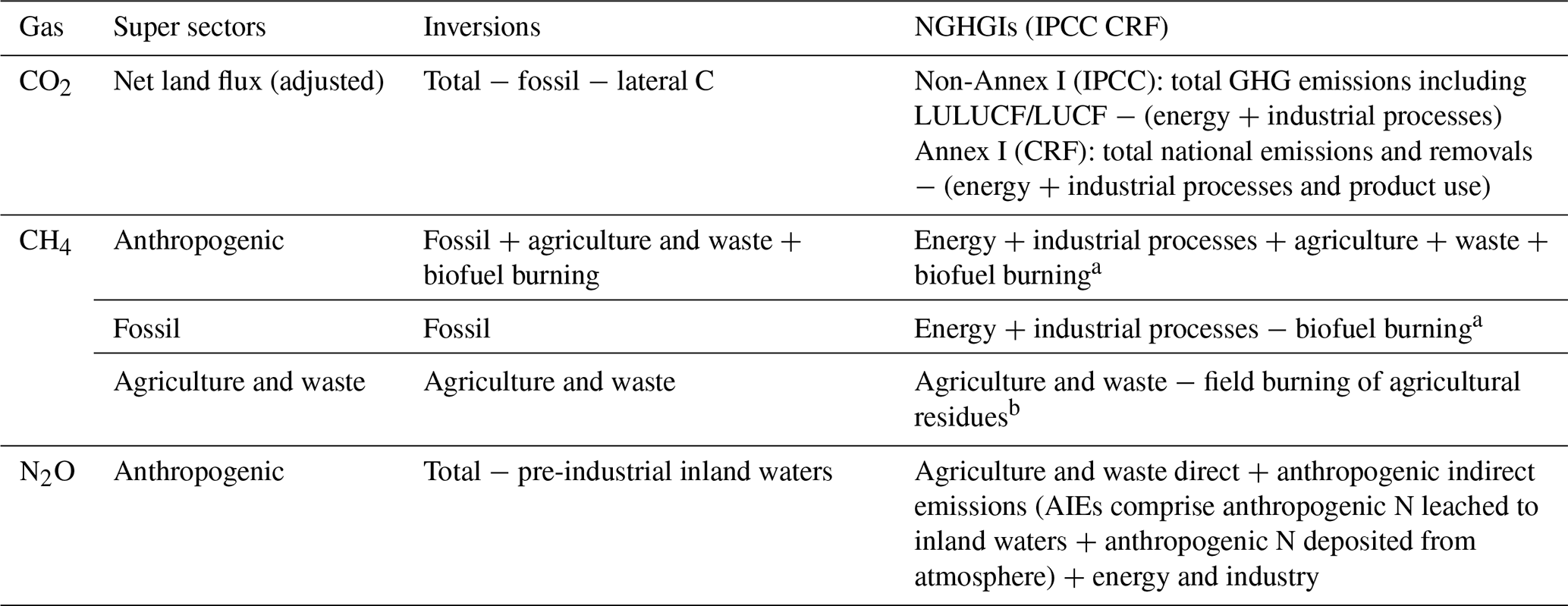
^a Biofuel burning is likely not included in NGHGIs but is under “1.A.4 Other Sectors” if it is reported. ^b Field burning of agricultural residues is reported in Annex I countries under the agricultural sector. Note that indirect N₂O emissions are reported by Annex I countries but not systematically by non-Annex I ones.

2.7 Choice of example countries for analysis

For the analysis, we selected 12 countries (or groups of countries) based on specific criteria for each aggregated sector (Table 5). Firstly, each chosen country had to possess a sufficiently large land area, as the limitations of coarse-spatial-resolution inversions make it difficult to reliably estimate GHG budgets for smaller countries. Additionally, it was preferable for the selected countries to have some coverage provided by the in situ global network of monitoring stations.

For CO₂, we focus on the land CO₂ fluxes of large fossil fuel CO₂ emitters. Although inversions do not allow us to verify fossil emissions in these countries as they are used as a fixed prior map of emissions, it is crucial to compare the magnitude of national land CO₂ sinks with fossil fuel CO₂ emissions in those large emitters. It is important to note that fitting net fluxes to changes in atmospheric CO₂ and then subtracting the prior fossil fuel (FF) fluxes can result in errors in the residual values, which are typically attributed exclusively to the sum of all non-FF fluxes. Additionally, we included two large boreal forested countries (Russia – RUS and Canada – CAN), two tropical countries with large forest areas (Brazil – BRA and the Democratic Republic of Congo – COD), two large countries with ground-based stations (Mongolia – MNG and Kazakhstan – KAZ), and two large dry Southern Hemisphere countries also with high rankings in fossil fuel CO₂ emissions (South Africa – ZAF and Australia – AUS), the latter of which both possess atmospheric stations to constrain their land CO₂ flux.

For CH₄, we first ranked countries (or groups of countries) based on their total anthropogenic, fossil, and agricultural emissions. This study includes China (CHN), India (IND), the United States (USA), the European Union (EUR), Russia (RUS), Argentina (ARG), and Indonesia (IDN), all of which are among the top emitters of both fossil fuel and agricultural CH₄ and possess large areas. Criteria of large land areas and the presence of atmospheric stations are crucial for in situ inversions. The advantage of utilizing GOSAT in CH₄ atmospheric inversions is its ability to provide observations over countries where surface in situ data are sparse or absent, such as in the tropics. This allows us to consider countries with limited or few ground-based observations. Small countries were excluded due to the coarse spatial resolution. However, among the selected countries, Venezuela, with an area of 916 400 km², was chosen specifically for the analysis of CH₄ emissions. Despite being relatively small, Venezuela is a large producer of oil and gas, potentially allowing for inversions using GOSAT observations to constrain its emissions. In major oil- and gas-extracting countries that have negligible agricultural and wetland emissions like Kazakhstan (KAZ), grouped in this study with Turkmenistan (TKM) into KAZ&TKM; Iran (IRN); and Persian Gulf countries (GULF), fossil emissions should be easier to separate by inversions and thus easier to compare with NGHGIs.

For N₂O, we selected the top 12 emitters based on the NGHGI reports. Anthropogenic N₂O emissions in most of these countries are predominantly driven by the agricultural sector, which accounts for a share (including indirect emissions) ranging from 6 % in Venezuela (VEN) to 95 % in Brazil (BRA) of their total NGHGI emissions.

Together, the selected countries (or groups of countries), with a different selection for each gas, account for more than 90 % of the global land CO₂ sink, 60 % of the global anthropogenic CH₄ emissions (around 15 % of fossil fuel emissions and approximately 40 % of agriculture and waste emissions separately), and 55 % of the global anthropogenic N₂O emissions, as estimated by the NGHGIs.

Table 5 Lists of countries or groups of countries are analyzed and displayed in the result section for each aggregated sector: Argentina (ARG); Australia (AUS); Brazil (BRA); Bangladesh (BGD); Canada (CAN); China (CHN); Columbia (COL); the Democratic Republic of the Congo (COD); Indonesia (IDN); India (IND); Iran (IRN); the European Union (EUR); Kazakhstan (KAZ); Mexico (MEX); Mongolia (MNG); Nigeria (NGA); Pakistan (PAK); Russia (RUS); South Africa (ZAF); Sudan (SDN); Thailand (THA); the United States (USA); Venezuela (VEN); Saudi Arabia, Oman, the United Arab Emirates, Kuwait, Bahrain, Iraq, and Qatar (GULF); and Kazakhstan and Turkmenistan (KAZ&TKM). For CH₄, abbreviations in bold denote the countries that appear in both the anthropogenic and the fossil or agriculture and waste sectors.

3 Results for net land CO₂ fluxes

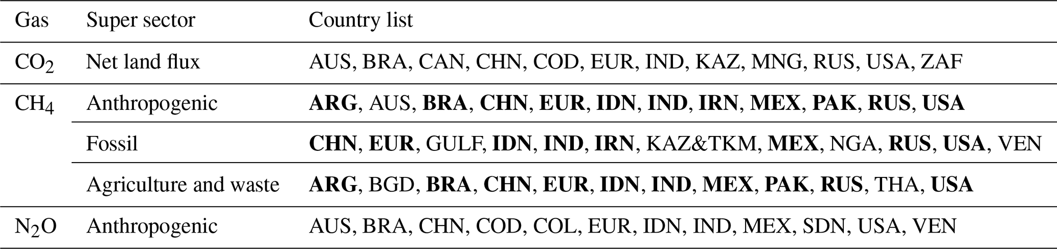
Figure 3 presents the time series of land-to-atmosphere CO₂ fluxes for the selected countries listed in Table 5. The median of inversions across the 12 countries shows significant interannual variability, reflecting the impact of climate variability on terrestrial carbon fluxes and annual variations in land-use emissions. In this paper, for inversion results covering a time interval, we present the data as mean ± standard deviation, where the mean is the multi-year average of the median flux values from the inversion models and the standard deviation represents the interannual variability.

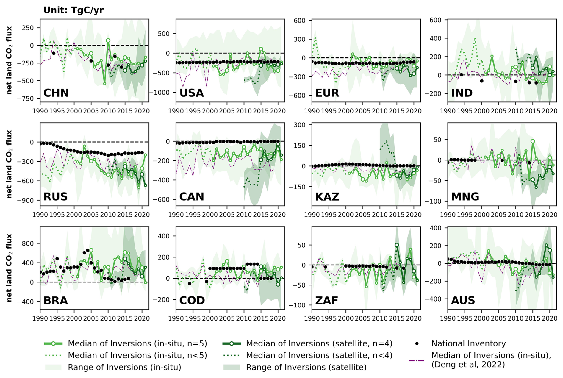
Figure 3 Net land CO₂ fluxes (unit: Tg C yr⁻¹) during 1990–2021 from China (CHN), the United States (USA), the European Union (EUR), India (IND), Russia (RUS), Canada (CAN), Kazakhstan (KAZ), Mongolia (MNG), Brazil (BRA), the Democratic Republic of the Congo (COD), South Africa (ZAF), and Australia (AUS). By convention, CO₂ removals from the atmosphere are counted negatively, while CO₂ emissions are counted positively. The black dots denote the reported values from NGHGIs. The light-green color denotes the in situ-alone CO₂ inversion (n=5) set, while the dark-green color denotes the set that uses satellite data (n=4). The green lines denote the median of land fluxes over managed land of CO₂ inversions, after adjustment of CO₂ fluxes from lateral transport by rivers, crop, and wood trade. When all inverse models within the inversion sets (in situ: n=5; satellite: n=4) have available data for the same time interval, their median values are depicted as solid green lines. Otherwise, when the inversion sets have incomplete inverse models within the time interval (in situ: n<5; satellite: n<4), their median values are represented as dashed green lines. Besides, before 2015, only GOSAT was available for two of the four satellite-based inversions until September 2014, when the OCO-2 record started. The shaded area denotes the min–max range of inversions. The dash-dotted purple lines denote the median of inversions presented by the previous study (Deng et al., 2022).

The adjustments of lateral CO₂ flux generally tend to lower land carbon sinks or increase land carbon emissions, especially in China (CHN), the United States (USA), the European Union (EUR), Russia (RUS), Canada (CAN), India (IND), and Brazil (BRA). In these countries, adjusting inversions by CO₂ fluxes induced by river carbon transport and by the trade of crop and wood products tends to lower CO₂ sinks, especially for large crop exporters like the USA and CAN. The adjusted net lateral transport fluxes for these countries are 48 (CHN), 143 (USA), 86 (EUR), 63 (RUS), 72 (CAN), 75 (IND), and 145 (BRA) Tg C yr⁻¹, which represent 20 %, 38 %, 48 %, 11 %, 41 %, 94 %, and 60 %, respectively, of the managed-land CO₂ fluxes before lateral transport adjustments. However, even with these adjustments, in countries of temperate latitudes, the median values of the five in situ-alone inversion ensembles all indicate a net carbon sink during the 2010s: CHN with a sink of 180 ± 100 Tg C yr⁻¹, the USA with 210 ± 180 Tg C yr⁻¹, EUR with 90 ± 50 Tg C yr⁻¹, RUS with 490 ± 100 Tg C yr⁻¹, and CAN with 110 ± 40 Tg C yr⁻¹. In CHN, despite only five values reported to the UNFCCC, NGHGIs show good agreement with the inversion results, with both NGHGIs and inversions exhibiting an overall increase in the carbon sink over the study period. However, during 2015–2021, the median values of the satellite-based inversion ensemble show a higher carbon sink of 320 ± 60 Tg C yr⁻¹ compared to those from in situ inversion results (220 ± 50 Tg C yr⁻¹) in CHN. In IND, there are also only five reported estimates from the NGHGIs. The in situ inversion results indicate that India exhibited fluctuations between being a carbon source and a carbon sink during the period of 2001–2014 (40 ± 70 Tg C yr⁻¹). During 2015–2019, the in situ inversion results in IND show a median carbon sink of 65 ± 20 Tg C yr⁻¹; however, the median reverted to being a carbon source of 90 Tg C yr⁻¹ (ranging from a sink of 350 to a source of 260 Tg C yr⁻¹) in 2020. In contrast, the median values of the satellite-based inversion ensemble indicate a carbon source of 65 ± 64 Tg C yr⁻¹ during 2015–2021 in IND.

As Annex I countries, the USA, EUR, RUS, CAN, and Kazakhstan (KAZ) have continuously reported annual NGHGIs since 1990. The NGHGI-reported values for the USA and CAN indicate a declining trend (Mann–Kendall $Z=-\mathrm{0.6}$, p<0.01) of carbon sinks by an annual average rate of 0.7 and 0.5 Tg C yr⁻², respectively. Like in Deng et al. (2022), we found that the carbon sink of Canada's managed land is significantly larger ($-\mathrm{130}\pm \mathrm{50}$ Tg C yr⁻¹ over 2001–2021 from in situ inversions) than that of the NGHGI reports (5 ± 4 Tg C yr⁻¹ over 2001–2021). Part of this difference could be due to the fact that Canada decides in its inventory not to report fire emissions as they are considered to have a natural cause. In doing so, Canada also excludes recovery sinks after burning, and those recovery sinks could surpass, on average, fire emissions, although remote sensing estimates of post-fire biomass changes suggest that fire emissions exceeded regrowth on average in western Canada and Alaska until ∼ 2010 (Wang et al., 2021). One reason for the difference may be that the NGHGI used old growth curves for forests, potentially underestimating the actual forest growth. Another reason for the difference may be shrubland and natural peatland carbon uptake and possibly an underestimated increase in soil carbon in the national inventory. For the USA we have good agreement between inversions (−290 ± 180 Tg C yr⁻¹ for in situ inversions over 2001–2021) and the NGHGI data (−220 ± 10 Tg C yr⁻¹ over 2001–2021), with the inversion showing much more interannual variability and the USA being a net source of carbon in the years 2011, 2015, and 2016 from the median of in situ inversions. The lower variability in the NGHGI data reflects the 5-year averaging of C stock changes by the national forest inventory. In EUR, the new in situ inversion ensemble gives a lower carbon sink than the previous one (purple line in Fig. 3; see discussion in Sect. 6.1), now being in good agreement with NGHGIs (−80 ± 60 Tg C yr⁻¹ compared to −85 ± 10 Tg C yr⁻¹) over 2001–2021. The OCO-2 satellite inversions give a higher sink than in situ inversions by $-\mathrm{200}\pm \mathrm{80}$ Tg C yr⁻¹, possibly because the in situ surface network does not cover eastern European countries, which have a larger NEE than western European ones, whereas OCO-2 data have a more even coverage of the continent, as discussed by Winkler et al. (2023) (see their Fig. 2, showing that OCO-2 inversions have a similar NEE to in situ ones in western Europe but a larger mean NEE uptake in eastern Europe).

In contrast, the NGHGIs in RUS report a rapid trend of an increasing sink by a rate of 4.6 Tg C yr⁻² (Mann–Kendall Z=0.69, p<0.01) during 1990–2020, supported by the significant strong correlation with the medians of the in situ inversion ensemble (ρ=0.7, p<0.01) during 2001–2020. However, the median values for both the in situ (480 ± 100 Tg C yr⁻¹) and the satellite-based (450 ± 90 Tg C yr⁻¹) inversion ensemble over RUS indicate larger land carbon sinks than those reported in the NGHGIs (180 ± 10 Tg C yr⁻¹) during 2011–2020. For KAZ, the NGHGIs suggest that managed land is a slight carbon source (6 ± 5 Tg C yr⁻¹) during 2000–2020. However, the median values for both the satellite-based and the in situ inversion ensemble indicate a carbon sink of 50 ± 30 Tg C yr⁻¹ and 60 ± 30 Tg C yr⁻¹, respectively, during 2015–2021 and 2001–2021. It is worth noting that the satellite-based inversion results for the USA, CAN, and KAZ all exhibit shifts in their fluxes between 2010 and 2015 compared to the results after 2015. This is attributed to the use of different satellite data and the number of different ensembles during these periods. Before 2015, only GOSAT was available, and only two out of four systems were available. After the OCO-2 record started, in September 2014, the satellite-driven inversion set only assimilated OCO-2. This indicates that inversion results based on GOSAT data are not consistent at the country scale with OCO-2 inversions. As a result, we can compare OCO-2 inversions with NGHGIs since 2015 but not the trends from inversions using GOSAT and/or OCO-2 inversions since 2009.

In BRA, both the NGHGI reports (240 ± 170 Tg C yr⁻¹ during 1990–2016) and inversion results (in situ: 350 ± 190 Tg C yr⁻¹ during 2001–2021; satellite-based: 280 ± 120 Tg C yr⁻¹ during 2015–2021) indicate that the country has been a net carbon source since 1990. The carbon source from managed land in Brazil increased from the late 1990s, reaching a peak in around 2005 according to NGHGIs (677 Tg C yr⁻¹). This evolution is confirmed by in situ inversions with a source peaking in 2005 (∼ 650 Tg C yr⁻¹). The net carbon source from inversions then decreased from 2005 to 2011, which is consistent with the observed reduction in deforestation due to forest protection policies implemented by the Brazilian government. This is an encouraging result as the inversions did not explicitly consider land-use emissions in their prior assumptions, although some included an estimate of carbon released by fires in their prior which is part of land-use emissions in Brazil. Since NEE is defined as all land fluxes except fossil fuel emissions, NEE from all inversions nevertheless include land-use emissions from deforestation; degradation emissions; and fire emissions including fires from deforestation, degradation, and other fires. After 2011, inversions show a new increase in land emissions, with a peak during the 2015–2016 El Niño. There have been higher average land emissions since. These ongoing changes may be attributed to various factors such as the legacy effects of drought leading to increased tree mortality (Aragão et al., 2018), higher wildfire emissions (Naus et al., 2022; Gatti et al., 2023), carbon losses from forest degradation, and climate-change-induced reductions in forest growth due to regional drying and warming in the southern and eastern parts of the Amazon (Gatti et al., 2021). From 2011 to 2016, the NGHGI reports indicate that carbon emissions from Brazilian managed lands were stable at around 47 Tg C yr⁻¹. However, the medians of in situ inversions suggest that carbon emissions rapidly increased from ∼ 100 Tg C yr⁻¹ in 2011 to ∼ 600 Tg C yr⁻¹ in 2016, which peaked in 2015 (∼ 610 Tg C yr⁻¹). From 2016 to 2021, the medians for both in situ and satellite inversion results show a decrease in carbon emissions from 2016 to 2018 but a transient peak in 2019, a year with large fires (Gatti et al., 2023) (in situ: 480 Tg C yr⁻¹; satellite: 270 Tg C yr⁻¹). Then carbon emissions decreased again until 2021, which experienced wetter conditions and fewer fires (Peng et al., 2022). The in situ inversion results show a continuous decrease to −10 Tg C yr⁻¹ in 2021, while the satellite inversion results showed a persistent source carbon anomaly of 300 Tg C yr⁻¹. We emphasize moreover that available CO₂ observations from a network of aircraft vertical sampling (Gatti et al., 2021) were not used to constrain the inverse models used here.

For the Democratic Republic of the Congo (COD), the available NGHGI data indicate that before 2000, the country's managed lands were a net carbon sink (50 Tg C yr⁻¹ in 1994 and 30 Tg C yr⁻¹ in 1999). Since 2000, the NGHGI reports have indicated three stages of different levels of CO₂ flux, whereby COD managed land was a carbon source during 2000–2010 (∼ 95 Tg C yr⁻¹), a larger carbon source during 2011–2014 (∼ 135 Tg C yr⁻¹), and a very small sink during 2015–2018 (∼ −1 Tg C yr⁻¹). The medians of the in situ inversion ensemble indicate a similar annual average carbon source (70 ± 45 Tg C yr⁻¹) during 2001–2021 with the NGHGIs, despite the low number of observations over Africa (Byrne et al., 2023). In the last decade, satellite inversion results from 2015 to 2021 have indicated a smaller source (30 ± 55 Tg C yr⁻¹) compared to the in situ results (85 ± 25 Tg C yr⁻¹). Moreover, the satellite inversion results indicate a sink anomaly in 2020 (−60 Tg C yr⁻¹) which is not found in the in situ inversions. The sink anomaly in 2020 from the satellite inversions is consistent with wetter conditions during that year over COD.

For South Africa (ZAF), the NGHGIs show a very small stable sink of 3 Tg C yr⁻¹ during 1990–2010, which doubled from 4 Tg C yr⁻¹ in 2010 to 8 Tg C yr⁻¹ in 2017, while the in situ inversion results indicate large fluctuations from a carbon sink (especially peaked in 2006, 2009, 2011, 2017, and 2021) to a small carbon source (e.g., in 2013 and 2018–2019). From 2015 to 2021, the satellite-based inversion results are consistent with the in situ results for annual variability (ρ=0.8, p<0.05), which is a good sign of the consistency between different atmospheric observing systems. During the transition to El Niño conditions and drought from 2014 to 2015, however, the satellite-based inversion results indicate a switch from a carbon sink to a source anomaly of 50 Tg C yr⁻¹ in ZAF which is not seen in the in situ inversions.

In Australia (AUS), the NGHGI data show a land source of carbon from 1990 to 2012, which decreased over time (from 48 Tg C yr⁻¹ in 1990 to 1 Tg C yr⁻¹ in 2012) and changed into a carbon sink from 2013 (which increased from a sink of 1 Tg C yr⁻¹ in 2013 to 15 Tg C yr⁻¹ in 2020). However, the in situ inversions indicate fluctuations between a carbon source and a sink with a small annual average sink of 10 ± 71 Tg C yr⁻¹ observed over the period of 2001–2021; except for in 2009–2011, the medians of in situ inversions reveal a strong carbon sink of 105 ± 35 Tg C yr⁻¹. Between 2010 and the strong La Niña year of 2011, the medians of the in situ inversion ensemble from the previous study (Deng et al., 2022) showed an increase in carbon uptake of 145 %. This high carbon sink persisted in 2012, which was a drier year with maximum bushfire activity. However, in this study, the medians of the updated in situ inversion ensemble indicate that there is a sink anomaly in 2011 followed by a source anomaly in 2013, which appears to be more realistic. The year of 2019 was the driest and hottest year recorded in Australia, including extreme fires at the end of 2019 (Byrne et al., 2021). As a result, the medians for both the in situ and the satellite inversion ensemble show a carbon source anomaly in 2019, with 55 Tg C yr⁻¹ (ranging from a sink of 1060 to a source of 480 Tg C yr⁻¹) and 200 Tg C yr⁻¹ (ranging from a sink of 120 to a source of 320 Tg C yr⁻¹), respectively. When it comes to the wet La Niña year of 2021, the medians for both the in situ and the satellite inversion ensemble indicate that AUS managed land became a carbon sink of 130 Tg C yr⁻¹ (ranging from a sink of 1120 to a source of 25 Tg C yr⁻¹) and 150 Tg C yr⁻¹ (ranging from a sink of 260 to a source of 40 Tg C yr⁻¹).

Last, we give the global comparison between NGHGIs and inversions, using NGHGI data compiled for all countries by Grassi et al. (2023), which include Annex I countries reports and non-Annex I NCs, BURs, and NDCs. The river correction is the only one that changes the global NEE because the global mean of CO₂ fluxes from wood and crop products is close to zero. The river-induced CO₂ uptake over land that is removed from inversion NEE is equal to the C flux transported to the ocean at river mouths (0.9 Gt C yr⁻¹ in our estimate, close to the value of Regnier et al., 2022). The (in situ) inversions without the river correction give a global NEE sink of 1.8 Gt C yr⁻¹ over 2001–2020 (managed land: 1.3 Gt C yr⁻¹ (72 % of total); unmanaged land: 0.5 Gt C yr⁻¹ (28 %)). The in situ inversions with the river correction study give a global NEE sink of 0.91 Gt C yr⁻¹ (managed land: 0.51 Gt C yr⁻¹ (56 % of total); unmanaged land: 0.4 Gt C yr⁻¹ (44 % of the total)). This is an important update from Deng et al. (2022), where the river CO₂ flux correction was not applied separately to managed and unmanaged lands. Because managed lands have a much larger area than unmanaged ones and because the spatial patterns of the CO₂ sinks in the river correction are distributed with MODIS net primary production (NPP), which has low values in unmanaged lands of northern Canada and Russia, the river correction strongly reduces the C storage change with respect to NEE over managed lands and marginally reduces it in unmanaged lands. Inventory data recently compiled by Grassi et al. (2023) indicate a similar global land sink (on managed land) of 0.53 Gt C yr⁻¹ with gap-filled data during the same period as the inversions with our improved river correction.

4 Results for anthropogenic CH₄ emissions

4.1 Total anthropogenic CH₄ emissions

Figure 4 presents the variations in anthropogenic CH₄ emissions for the 12 selected countries, where these emissions sum the sectors of agriculture and waste, fossil fuels, and biofuel burning. The distribution of emissions is highly skewed even among the top 12 emitters, with the largest and most populated countries/regions such as China (CHN), India (IND), the United States (USA), Brazil (BRA), Russia (RUS), and the European Union (EUR) which emits more than 10 Tg CH₄ yr⁻¹ annually, while other countries have smaller emissions (ranging from 3 to 10 Tg CH₄ yr⁻¹) that are more challenging to quantify through inversions. During 2010–2020, CHN has the highest total anthropogenic emissions at around 50 ± 4 Tg CH₄ yr⁻¹, followed by IND with 30 ± 1 Tg CH₄ yr⁻¹, the USA with 24 ± 1 Tg CH₄ yr⁻¹, BRA with 24 ± 1 Tg CH₄ yr⁻¹, EUR with 19 ± 1 Tg CH₄ yr⁻¹, Indonesia (IDN) with 14 ± 1 Tg CH₄ yr⁻¹, and RUS with 13 ± 1 Tg CH₄ yr⁻¹, according to the medians of the satellite-based inversion ensemble based on EDGAR v6.0 as prior. The remaining countries have emissions of approximately 5 Tg CH₄ yr⁻¹. In general, the difference between NGHGIs and inversions aligns in the same direction based on both satellite and in situ inversions. This provides some confidence in using inversions to evaluate NGHGIs as the satellite observations are independent from in situ networks. Overall, satellite-based inversions may be more robust across most countries due to better observation coverage, except in EUR and the USA, where the in situ network is more extensive.

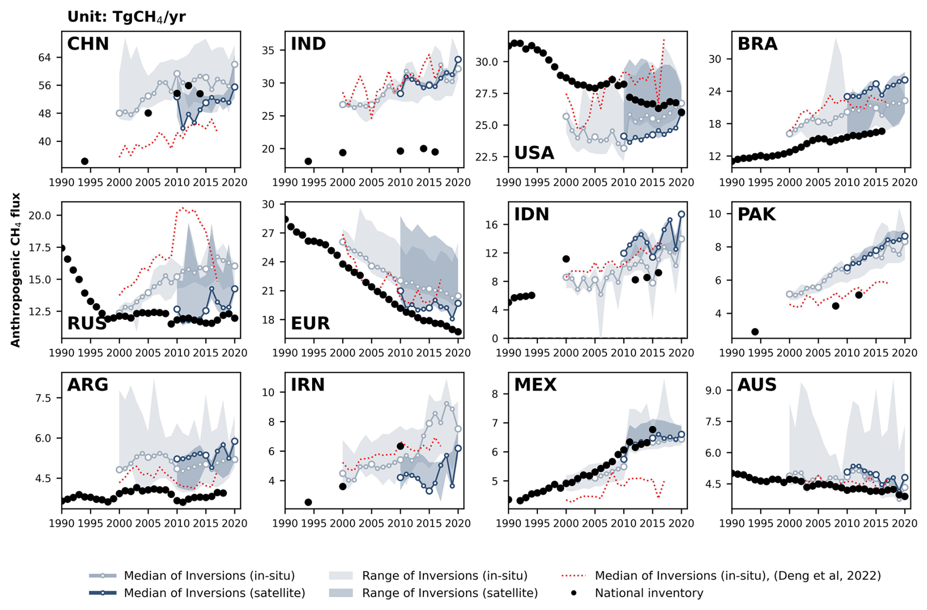
Figure 4 Total anthropogenic CH₄ fluxes for the 12 top emitters: China (CHN), India (IND), the United States (USA), Brazil (BRA), Russia (RUS), the European Union (EUR), Indonesia (IDN), Pakistan (PAK), Argentina (ARG), Iran (IRN), Mexico (MEX), and Australia (AUS). The black dots denote the reported values from NGHGIs. The light- and dark-blue lines and areas denote the median and maximum–minimum ranges of in situ and satellite-based CH₄ inversions based on EDGAR v6.0 as the prior, respectively. Developing countries, such as CHN, IND, BRA, IDN, Pakistan (PAK), Iran (IRN), and Mexico (MEX), show a rapid increase in anthropogenic CH₄ emissions supported by reported values from NGHGIs and results from inversions. In CHN, the reported values from NGHGIs (when available) generally align with the results obtained through inversions (e.g., during 2010–2015, 54 ± 1 Tg CH₄ yr⁻¹ for NGHGIs, 58 ± 1 Tg CH₄ yr⁻¹ for in situ, 48 ± 3 Tg CH₄ yr⁻¹ for satellite-based). During 2010–2020, the median values for the in situ and satellite-based inversion ensemble show a similar increasing trend at an annual growth rate of 0.28 and 0.26 Tg CH₄ yr⁻², respectively, although the medians of in situ inversion ensemble (58 ± 2 Tg CH₄ yr⁻¹) were slightly higher than the satellite-based ensemble (50 ± 3 Tg CH₄ yr⁻¹). However, in 2020, the medians of the emission estimates for both in situ and satellite-based inversions reveal a rapid increase by 9 % and 11 % compared to 2019 in CHN, indicating a possible surge in anthropogenic methane emissions for that year that is possibly an artifact from the fact that the decreased OH sink in 2020 is not well accounted for here. Indeed OH interannual variability was not prescribed in all inversions, and when accounted for, the OH interannual variability prescribed (based on Patra et al., 2022) was much smaller than the values suggested by recent studies (e.g., Peng et al., 2022). As a result, overestimating the sink in the inversions leads to overestimated surface emissions. The surge in emissions could also be due to spin-down, the last 6 months to 1 year of inversions being less constrained by the observations even though the inversion period covered up to June 2021.

In IND, PAK, and MEX, there is good agreement (r>0.8, p<0.01) between the in situ and satellite-based inversion ensembles (31 ± 1 and 30 ± 1 Tg CH₄ yr⁻¹ in IND, 8 ± 1 and 7 ± 1 Tg CH₄ yr⁻¹ in PAK, and 6 ± 1 and 6 ± 1 Tg CH₄ yr⁻¹ in MEX, respectively), while both of them present a significant increasing trend of anthropogenic methane emissions in these countries (Mann–Kendall p<0.05). However, when comparing to NGHGI values, the inversion results in IND and PAK indicate > 50 % larger emissions than those reported from the NGHGIs during 2010–2020. In contrast, values reported from the NGHGIs (∼ 6 Tg CH₄ yr⁻¹) by MEX also show good agreement with the inversion results.

In BRA, IDN, and Argentina (ARG), the medians for in situ and satellite-based inversion ensembles show good consistency (r=0.8, p<0.01) in these two countries, while satellite-based inversion results are generally higher than the in situ inversion results. Specifically, in BRA, the satellite-based inversions (24 ± 1 Tg CH₄ yr⁻¹) were 16 % higher than the in situ inversions (21 ± 1 Tg CH₄ yr⁻¹) and 52 % higher than the NGHGI estimation (∼ 17 Tg CH₄ yr⁻¹) during 2010–2020, possibly owing to difficulties in inversions differentiating between natural (wetlands, inland waters) and anthropogenic sources in this country and to possible flaws in the prior used for natural and anthropogenic fluxes. In IDN, NGHGIs reported a significant continuous upward trend at an annual average growth of 0.3 Tg CH₄ yr⁻¹, with a noticeable positive outlier in 2000. The medians for both in situ and satellite-based inversion ensembles also indicate an upward trend in IDN, but both of them present sudden dips in anthropogenic methane emissions in 2015 and 2019 by 15 %–23 % and 16 %–25 % compared to the previous year, respectively. It is unlikely that anthropogenic activities could contribute such large year-to-year variations except for different flooded areas used for rice paddies. In ARG, the satellite-based inversion results also indicate two sudden dips in 2016 and 2019; however, such a pattern was not found in the in situ inversion results. A cause of year-to-year variations from inversions is the lack of in situ sites and variable cloud cover affecting the density of GOSAT data.

Regarding IRN, NGHGIs only provided data for three years (1994, 2000, and 2010), making it difficult to compare them with inversion results. However, NGHGIs show a rapid growth in anthropogenic CH₄ emissions (+9.4 % yr⁻¹) during this period. There are significant differences between inversion results and for IRN, with satellite inversions generally giving lower emissions than in situ inversions and different trends. Satellite inversions suggest a declining trend between 2010 and 2015, followed by a fluctuating increase until 2020. In contrast, in situ-based inversions (by any nearby measurement stations, thus likely reflecting the prior trend) show a rapid rise in emissions after 2010, reaching a peak in 2018, followed by a decline.

NGHGIs for RUS indicate that anthropogenic CH₄ emissions have been reduced during the 1990s and remained stable since 2000 (12.0 ± 0.3 Tg CH₄ yr⁻¹ during 2000–2020), which is similar with the trend observed from satellite-based inversion results (12.7 ± 0.9 Tg CH₄ yr⁻¹ during 2000–2020). However, in 2016, there was a sudden increase in emissions in satellite inversion results (+14 % increase from 12.5 Tg CH₄ yr⁻¹ in 2015 to 14.2 Tg CH₄ yr⁻¹ in 2016), followed by a gradual decline, and then a new increase in 2020 (+11 % increase from 12.8 Tg CH₄ yr⁻¹ in 2019 to 14.3 Tg CH₄ yr⁻¹ in 2020). This recent change was not observed in the in situ inversion results or the NGHGIs.

For the USA, Australia (AUS), and EUR, NGHGIs reported a slowly declining trend (EUR: 0.4 Tg CH₄ yr⁻¹; USA: 0.2 Tg CH₄ yr⁻¹; AUS: −0.04 Tg CH₄ yr⁻¹) in anthropogenic CH₄ emissions. In the case of the USA, inversion-derived emissions are slightly lower than NGHGIs (in situ-based: 9 % lower during 2000–2020; satellite-based: 11 % lower during 2010–2020). However, both ground-based and satellite-based inversions indicate that anthropogenic CH₄ emissions have remained relatively steady since 2000, without reflecting the slow decline reported by NGHGIs. In EUR, NGHGIs indicate that anthropogenic CH₄ emissions have been decreasing rapidly since 1990 (−1.4 % yr⁻¹), consistent with the trend obtained from inversion results. However, in situ inversion emissions are on average slightly higher than NGHGIs, and this difference has been gradually increasing from 8 % in the 2000s to 15 % in the 2010s.

4.2 Fossil CH₄ emissions

Figure 5 presents the fossil CH₄ emissions for the top 12 emitters from the fossil sector based on EDGAR v6.0 as the prior. The largest emitter is China (CHN), mainly from the subsector of coal extraction, followed by Russia (RUS) and the United States (USA). In CHN, the in situ (20 ± 2 Tg CH₄ yr⁻¹) and satellite inversion (17 ± 1 Tg CH₄ yr⁻¹) emissions in the 2010s are 24 % and 35 % lower, respectively, than in the NGHGIs (∼ 26 Tg CH₄ yr⁻¹). The NGHGIs in CHN suggest a decrease from 28 Tg CH₄ yr⁻¹ in 2012 to 24 Tg CH₄ yr⁻¹ in 2014. However, both in situ and satellite inversion results indicate there has been an increasing trend since 2018. In India (IND) and Indonesia (IDN), NGHGIs report a decreasing trend during the study period, while inversions suggest a rapid increase in IDN and a stable value in IND after a peak in 2012. In IND, satellite inversions suggest a peak of fossil CH₄ emissions during 2011–2012, which then dropped in 2013 and remained stable afterward. In IDN, both in situ and satellite inversions indicate a fluctuating trend, with a significant drop between 2015 and 2019. In RUS, both in situ and satellite inversion-based estimates of fossil fuel emissions are higher than those of NGHGIs and show an increasing trend, while NGHGIs report a decreasing trend. This discrepancy may be due to inversion problems for separating between wetland emissions and gas extraction industries both located in the Yamal Peninsula area or to leaks not captured in NGHGIs. In the USA, NGHGIs overall show a significant declining trend (Mann–Kendall $Z=-\mathrm{0.8}$, p<0.01). In situ inversion estimates of fossil fuel emissions are 26 % lower than NGHGIs during 2000–2010 and remained consistent until around 2011. Nearly all in situ inversions show a jump in fossil fuel emissions in 2011. In the European Union (EUR), both NGHGIs and inversion results demonstrate a consistent declining trend. However, starting from 2010, both in situ and satellite inversions are higher than results in NGHGI reports.

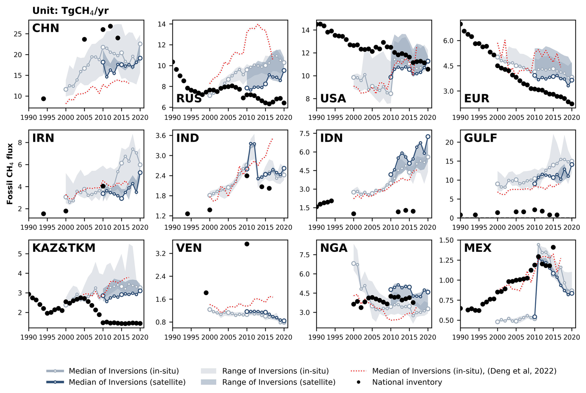
Figure 5 CH₄ emissions from the fossil fuel sector from the top 12 emitters of this sector: China (CHN), Russia (RUS), the United States (USA), the European Union (EUR), Iran (IRN), India (IND), Indonesia (IDN), Persian Gulf countries (GULF denotes Saudi Arabia, Iraq, Kuwait, Oman, the United Arab Emirates, Bahrain, and Qatar), Kazakhstan and Turkmenistan (KAZ&TKM), Venezuela (VEN), Nigeria (NGA), and Mexico (MEX). The black dots denote the reported value from the NGHGIs. In the NGHGI data shown for GULF, Saudi Arabia reported four NGHGIs in 1990, 2000, 2010, and 2012; Iraq reported one in 1997; Kuwait reported three in 1994, 2000, and 2016; Oman reported one in 1994; the United Arab Emirates reported four in 1994, 2000, 2005, and 2014; Bahrain reported three in 1994, 2000, and 2006; and Qatar reported one in 2007. The reported values are interpolated over the study period to be summed up and plotted in the figure. For KAZ&TKM, the reported values of Turkmenistan during 2001–2003, 2005–2009, and 2011–2020 are interpolated and added to annual reports from Kazakhstan, an Annex I country for which annual data are available. Other lines, colors, and symbols are as in Fig. 4.

Major oil-producing countries in the Persian Gulf are too small compared to the model resolution to be studied individually. Hence, NGHGIs from the GULF countries (Saudi Arabia, Iraq, Kuwait, Oman, the United Arab Emirates, Bahrain, and Qatar) were grouped and show much lower emissions compared to inversion results. In the 2010s, in situ and satellite inversions estimate that emissions in GULF were 9 times and 8 times higher, respectively, than the estimates reported in NGHGIs. This huge under-reporting of emissions in GULF could be partly attributed to the omission of ultra-emitters in NGHGIs. The ultra-emitters defined by Lauvaux et al. (2022) are all short-duration leaks from oil and gas facilities (e.g., wells, compressors) with an individual emission > 20 t CH₄ h⁻¹, each event lasting generally less than 1 d. Such leaks are often random occurrences and are difficult to quantify, which is why most countries do not account for these significant and episodic events in their national inventories. Indeed, recent studies by Lauvaux et al. (2022) have identified more ultra-emitters and larger emission budgets from ultra-emitters in Qatar, Kuwait, and Iraq. In KAZ&TKM, grouped together because of their rather small individual areas, both in situ (3 ± 0.2 Tg CH₄ yr⁻¹) and satellite (3 ± 0.1 Tg CH₄ yr⁻¹) inversions estimate emissions to be 2 times higher than NGHGIs (1.5 Tg CH₄ yr⁻¹) in the 2010s. Similarly, KAZ is located downwind of TKM, which has a high share of ultra-emitters. The global inversions operating at a coarse resolution may misallocate emissions from TKM to KAZ. It is worth noting that KAZ has two in situ stations for CH₄ measurements, whereas the GULF countries lack in situ station networks. On the other hand, GOSAT provides dense sampling of atmospheric column CH₄ in the Persian Gulf region due to frequent cloud-free conditions. Therefore, GOSAT inversions can be considered more accurate than in situ inversions for Iran (IRN), GULF countries, and Kazakhstan and Turkmenistan (KAZ&TKM). Additionally, it is important to note that GOSAT inversions generally give lower emissions than in situ inversions in those countries. Venezuela (VEN) is a rare case where NGHGIs report much higher CH₄ emissions than inversions. While the uncertainty in GOSAT inversions (model spread) has decreased compared to the results reported by Deng et al. (2022), the gap between inversions and NGHGIs has increased. In 2010, NGHGI reports of fossil CH₄ emissions in VEN were 298 % higher than those of GOSAT inversions and 326 % than those of in situ inversions. We do not have a clear explanation for this large difference, except that VEN has strongly decreased oil and gas extraction due to sanctions curbing its crude production from 2.7 million barrels d⁻¹ in 2015 to 0.6 million barrels d⁻¹ in 2020 (OPEC, 2023), which may not be reflected in their NGHGIs. In Nigeria (NGA) and Mexico (MEX), NGHGI estimates fall between the median of in situ and satellite inversions during 2010–2020. However, in MEX, the in situ inversion was 50 % lower than NGHGIs in the 2000s and showed a sudden large increase in 2010.

4.3 Agriculture and waste CH₄ emissions

Figure 6 presents CH₄ emissions of the agriculture and waste sector for the top 12 emitters of this sector. In all countries except for the United States (USA) and Russia (RUS), the values reported by NGHGIs are systematically lower than the inversion results. The results from the previous ensemble of in situ inversions (dotted red line) are consistent with those of the inversions used in this study except in the USA, where previous inversions are 3.2 Tg CH₄ yr⁻¹ higher; in RUS, where they show a drop after 2015 although they remain in the range from the new satellite and in situ inversions; and in Mexico (MEX), where they are systematically lower by 1.6 Tg CH₄ yr⁻¹.

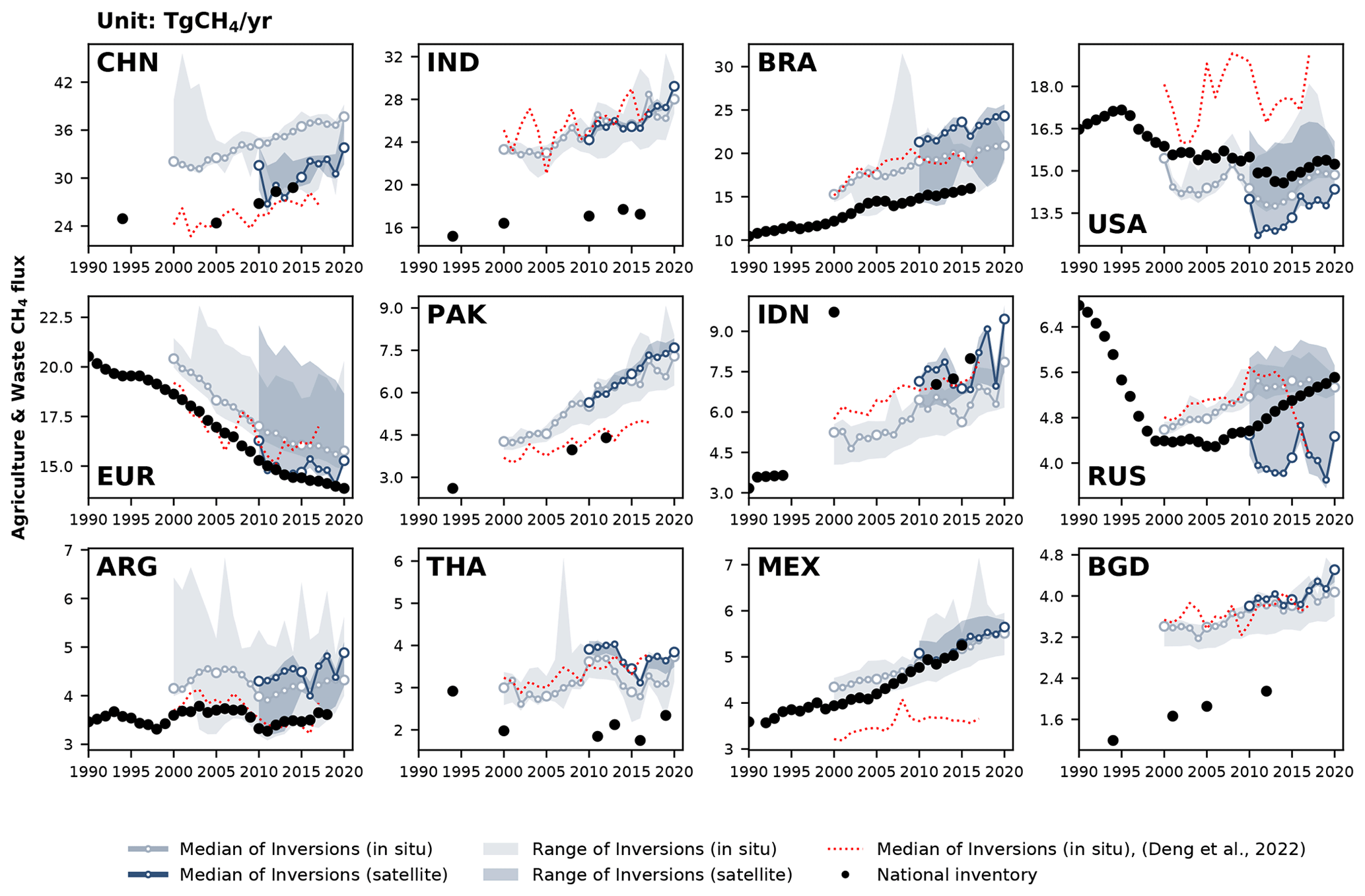
Figure 6 CH₄ emissions from agriculture and waste for the 12 largest emitters in this sector, China (CHN), India (IND), Brazil (BRA), the United States (USA), the European Union (EUR), Pakistan (PAK), Indonesia (IDN), Russia (RUS), Argentina (ARG), Thailand (THA), Mexico (MEX), and Bangladesh (BGD). The black dots denote the reported estimates from NGHGIs. Other lines, colors, and symbols are as in Fig. 4.

In China (CHN), the most recent NGHGI reports in 2012 and 2014 estimate agriculture and waste emissions at 28 Tg CH₄ yr⁻¹, which is close to the result of satellite inversions (28 ± 1 Tg CH₄ yr⁻¹) but 22.4 % lower than the median of in situ inversions (35 ± 1 Tg CH₄ yr⁻¹) and closer to their minimum value. The trend in agricultural and waste emissions is consistent between inversions and NGHGIs for CHN. In India (IND), inversions consistently show higher emissions than NGHGIs by approximately 50 % and indicate an increasing trend during 2000–2020, but with the NGHGI last communication being for 2016, we are not able to obtain a recent trend. According to the national inventory of IND, enteric fermentation is the primary source of CH₄ emissions in the agriculture and waste sector, contributing 61 % of emissions, with rice cultivation accounting for 20 % and waste contributing 16 %. A similar pattern is observed in Bangladesh (BGD), where agricultural emissions are dominated by rice production (48 % in 2012) and enteric fermentation (42 % in 2012). Satellite and in situ inversion estimate emissions in BGD are nearly double those reported by NGHGIs during 2001 and 2012, the year of the last communication. The significant discrepancies between inversions and NGHGIs in IND and BGD may be attributed to potential underestimation of livestock or waste CH₄ emissions by NGHGIs. NGHGIs utilized the Tier 1 method and associated emission factors from the 2006 IPCC Guidelines for National Greenhouse Gas Inventories (IPCC, 2006). However, a recent study (Chang et al., 2021) found that estimates using revised Tier 1 or Tier 2 methods from the 2019 Refinement to the 2006 IPCC Guidelines for National Greenhouse Gas Inventories (IPCC, 2019) give livestock emissions that are 48 %–60 % and 42 %–61 % higher for IND and BGD by 2010, respectively, compared to Tier 1 IPCC (2006) methods, which would bring bottom-up emissions closer to inversions. In Brazil (BRA), both satellite and in situ inversions consistently estimate larger emissions than the NGHGIs by 34 % and 29 %, respectively, and show a consistent increasing trend over their study periods. In the USA, the medians of satellite and in situ inversions are slightly lower than those of NGHGIs, but they exhibit a similar trend throughout the study period. The trend of inversions is comparable to the one of the NGHGIs in BRA during their period of overlap, although there is no NGHGI communication later than 2016. In Argentina (ARG), Pakistan (PAK), and Thailand (THA), the medians of in situ inversions show good consistency with satellite inversion results. Nevertheless, in situ inversion emissions in the 2010s are, on average, 47 % higher in PAK, 20 % higher in ARG, and 64 % higher in THA compared to the NGHGI reports. In the European Union (EUR), emissions from agriculture and waste were reported to have significantly decreased over time in the NGHGI data, mainly from solid waste disposal (Petrescu et al., 2021), a trend that is captured by inversions and is close to the one of the NGHGIs over the study period. In contrast, emissions from agriculture and waste in RUS are reported to have a positive trend after 2010 by the NGHGI, with in situ inversions producing a consistent trend from 2000 to 2014 but a sharp decrease thereafter, while satellite inversions produce stable emissions, although they are lower than those of the NGHGIs and in situ inversions after 2010.

5 Results for anthropogenic N₂O emissions

We present the 12 countries/regions with the largest anthropogenic N₂O emissions in the world (Fig. 7), which in total contribute approximately 55 % of global anthropogenic N₂O emissions. The estimates from both NGHGIs and inversions in China (CHN), the United States (USA), and the European Union (EUR) demonstrate a relatively close match between NGHGIs and inversions (in situ only). These three large emitting countries/regions exhibit different trends in their anthropogenic N₂O emissions. In CHN, both NGHGIs and inversions indicate an increasing trend in anthropogenic N₂O emissions. In the USA, anthropogenic N₂O emissions seem to have reached a state of relative stability, with NGHGIs and inversion results showing similar mean values and a lack of trends. In EUR, both NGHGIs and inversions show a declining trend in anthropogenic N₂O emissions, but from 2010 to 2020, the NGHGI estimates are lower (20 %) than the median values derived from inversion models; that is, the negative trend from inversions is less pronounced than the one of NGHGIs. Most other selected countries display higher anthropogenic N₂O emissions from inversions than from NGHGIs (i.e., Brazil (BRA), India (IND), the Democratic Republic of the Congo (COD), Indonesia (IDN), Mexico (MEX), Colombia (COL), Sudan (SDN), Venezuela (VEN)). These discrepancies in anthropogenic N₂O emissions are possibly attributable to factors that were analyzed in our previous study (Deng et al., 2022). Firstly, nearly all these non-Annex I countries utilize Tier 1 emission factors (EFs), which may underestimate emissions when soil and climate dependence are taken into account (Cui et al., 2021). This has been noted in previous studies (Philibert et al., 2013; Shcherbak et al., 2014; Wang et al., 2020). Furthermore, the observed concave response of cropland soil emissions as a function of added N fertilizers may also contribute to underestimated emissions in NGHGIs, as the relationship is non-linear and higher than the linear relation used by NGHGIs in Tier 1 approaches (Zhou et al., 2015). In an improved reporting framework, EFs should also account for both natural and anthropogenic components, as they cannot be distinguished through the field measurements from which EFs are derived. However, in practice, EFs are mostly based on measurements made in temperate climates and soils from established croplands with few “background” emissions. Consequently, there could be a systematic underestimation of default IPCC EFs from tropical climates and for recently established agricultural lands, for which the IPCC EFs also have a huge uncertainty of up to ±75 %–100 %. Another factor that might contribute to the discrepancy is the omission of emissions from reactive nitrogen contained in organic fertilizers (manure), for which NGHGIs do not provide specific details for non-Annex I reports. Lastly, anthropogenic indirect emissions (AIEs) from atmospheric nitrogen deposition and leaching of human-induced nitrogen additions to aquifers and inland waters are reported by Annex I countries using simple emission factors, but non-Annex I countries do not consistently report AIEs. However, in Australia (AUS), the gap between inversions and NGHGIs has even expanded compared to that reported in our previous study. We do acknowledge that the density of the N₂O in situ network in tropical countries and around AUS is so low that inversions are most likely attracted to their priors. The use of a lower prior could thus also be consistent with scarce atmospheric observations, and we have only a low confidence in N₂O inversion results for tropical countries and AUS.

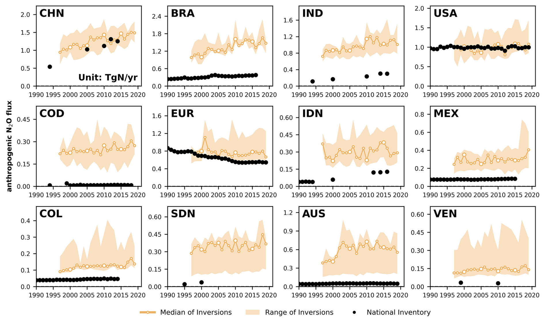
Figure 7 Anthropogenic N₂O fluxes of the top 12 emitters: China (CHN), Brazil (BRA), India (IND), the United States (USA), the Democratic Republic of the Congo (COD), the European Union (EUR), Indonesia (IDN), Mexico (MEX), Colombia (COL), Sudan (SDN), Australia (AUS), and Venezuela (VEN). The black dots denote the anthropogenic emissions from the UNFCCC national greenhouse gas inventories. The thick orange lines and the light-orange areas denote the median and the maximum–minimum ranges of anthropogenic fluxes, respectively, among all N₂O inversions. We restricted our analysis to data starting from 1997 because it was the year when data from all four inversion models become available.

6 Discussion

6.1 Comparing net land CO₂ flux estimates from different inversion model ensembles

In this section, we compare four different estimates of land CO₂ fluxes during the period 2010–2020 (Fig. 8), including (1) medians of in situ inversion results from our previous study (Deng et al., 2022), (2) medians of in situ and (3) satellite-based inversion results processed in this study based on the Global Carbon Budget 2022 (Friedlingstein et al., 2022), and (4) NGHGIs. This enables a comparison of the median and range of our in situ inversion results (n=5) with those from our previous study (n=6) and an assessment of the performance differences between satellite-based (n=4) and in situ inversion models. To ensure a fair comparison and avoid anomalies in the satellite-based inversion results during 2010–2015 when some of these inversions used GOSAT after 2010 and then OCO-2 after 2015, we separate the analysis into two periods: 2011–2015 and 2016–2020.

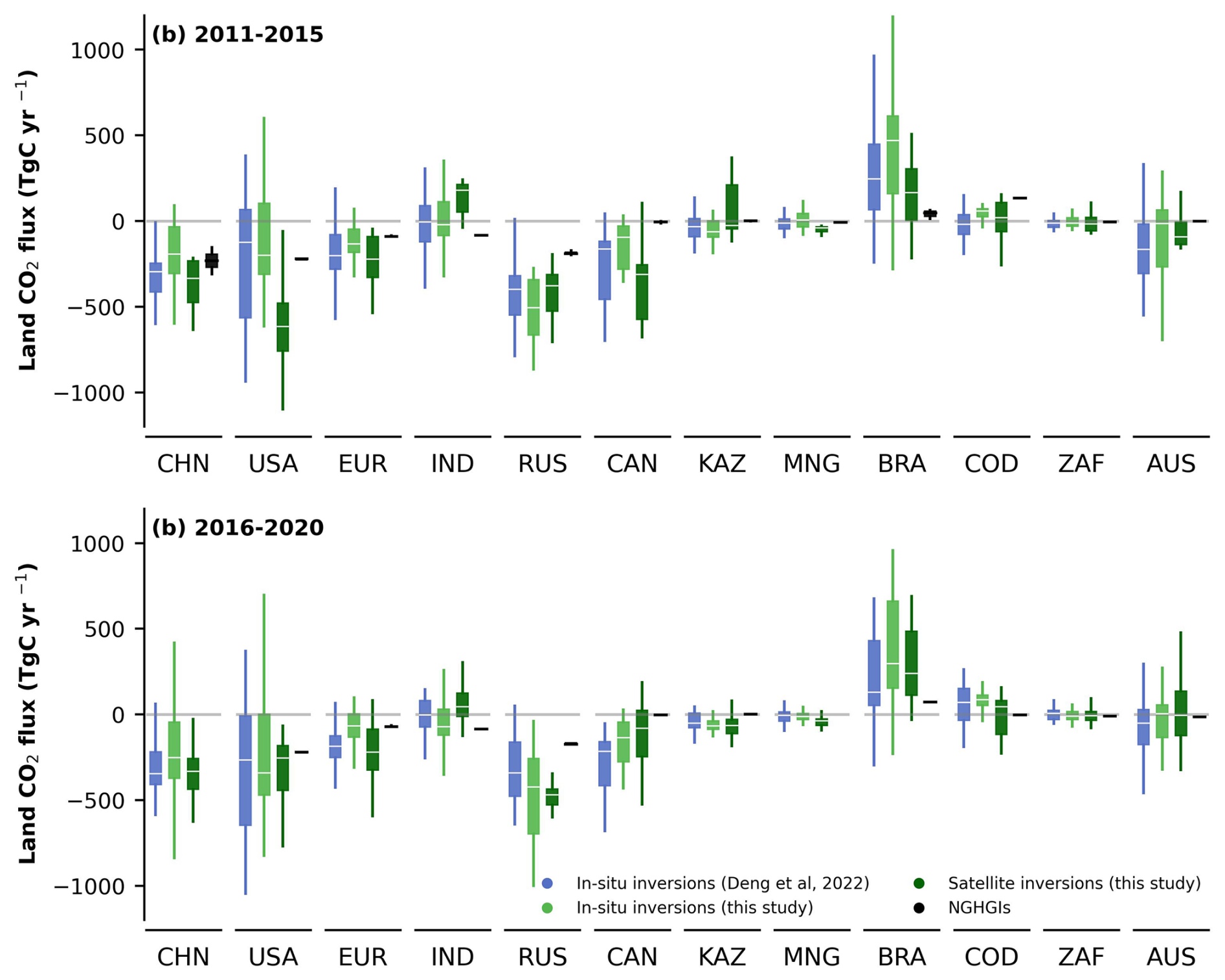
Figure 8 Net CO₂ land fluxes during the period of (a) 2011–2015 and (b) 2016–2020 in China (CHN), the United States (USA), the European Union (EUR), Russia (RUS), Canada (CAN), Kazakhstan (KAZ), Mongolia (MNG), India (IND), Brazil (BRA), the Democratic Republic of the Congo (COD), South Africa (ZAF), and Australia (AUS). Blue boxes denote the in situ inversion results from Deng et al. (2022) processed from the Global Carbon Budget 2020 (Friedlingstein et al., 2020). Light-green boxes denote the in situ inversion results processed in this study, while dark-green boxes denote the satellite inversion results. Black boxes denote the NGHGI-reported values. The white lines in the boxes denote the medians of the land CO₂ fluxes. Note that the inversion results here were adjusted by the lateral flux before the comparison. Additionally, we extend the comparison with national land-use change emissions from global bookkeeping models in Fig. S4.

The variations in yearly land CO₂ fluxes span a comparable range between the current and previous in situ inversion ensembles, indicating consistency of the inversion results but that the uncertainty within the new in situ inversion ensemble was not improved. However, examining the median values, results from the new in situ inversion ensemble may be closer to those of NGHGIs in most countries (such as China (CHN), the United States (USA), the European Union (EUR), Canada (CAN), Kazakhstan (KAZ), India (IND)). This suggests that the new in situ inversion ensemble used in this study has partially narrowed down the gaps between inversion results and NGHGIs compared to our previous study. However, in Russia (RUS) and Brazil (BRA), the difference between the median of in situ inversion ensembles and NGHGIs has enlarged. For example, in RUS, the new in situ inversion ensemble indicates a larger carbon sink than that from Deng et al. (2022), while the difference between the median of in situ inversions and NGHGIs increased 51 % during 2011–2015 (from 208 to 314 Tg C yr⁻¹) and 49 % during 2016–2020 (from 168 to 249 Tg C yr⁻¹). Conversely, in BRA, the median of the new in situ inversion ensemble indicates a larger carbon source, while the difference increased over 100 % during 2011–2015 (from 200 to 423 Tg C yr⁻¹) and nearly 300 % during 2016–2020 (from 56 to 223 Tg C yr⁻¹).

As for the inversion ensemble used in this study, in most countries, the variations in yearly land CO₂ fluxes also span a similar range between the satellite-based inversion ensemble and in situ inversion ensemble. However, in the cases of the USA, RUS, CHN, and BRA, the spread of satellite-based inversion results is narrower than that of in situ inversion results, indicating better consistency among available satellite-based inversion models, at least when similar satellite data are assimilated. In addition, in most cases, smaller differences were found between the median of inversion results and the NGHGIs. For countries with dense surface monitoring networks such as in the USA and EUR, the satellite-based inversion results show good agreement in terms of in situ inversion results. However, for countries with sparse station coverage like Kazakhstan (KAZ) and Mongolia (MNG), satellite-based inversion results could provide more reliable estimates due to more extensive spatial sampling from satellites, although the medians of satellite-based inversion results indicate larger carbon sinks and larger differences compared with NGHGIs (than for in situ inversion results). In the USA and CAN, the difference during 2011–2015 ( GOSAT-only period) between in situ and satellite-based inversion ensembles is larger than that during 2016–2020 (OCO-2 period). This can be attributed to the use of different satellite data during these periods and different numbers of ensemble members. Before 2015, only GOSAT and only two out of four systems were available. The inversion of OCO-2 data starting in 2014 resulted in a better alignment among ACOS OCO-2 v10 inversions, indicating the in situ and satellite evaluations were similar (Byrne et al., 2023).

6.2 Adjustment of the national managed-land masks to separate the net land CO₂ flux estimates

Following the method proposed by Grassi et al. (2023), in this study we updated the managed-land mask for Canada (CAN) and Brazil (BRA) using maps of managed land derived from NGHGIs and for Russia (RUS) by adjusting tree-cover threshold in the tree-cover map from Hansen et al. (2013) to match the average area of managed land per oblast (province) that is used for the NGHGIs. Thus, the new mask is now more consistent with the definition of managed land in the NGHGIs for these three countries, so we can further analyze the impacts of different definitions of managed-land masks to separate the managed-land CO₂ fluxes in inversions (Fig. 9). Generally, in Russia (RUS) and Canada (CAN), the managed-land CO₂ fluxes extracted from the new mask are closer to NGHGIs than those separated by the previous mask used by Deng et al. (2022). In addition, in Brazil (BRA), adjusting the national managed-land mask resulted in greater land carbon emissions, increasing the gap with NGHGIs. However, the improvement of the managed-land mask in this study is still not able to explain all the existing discrepancy between inversion estimates and NGHGIs, in which the sources of and reasons for these differences and uncertainties still need further analysis. We also observe in Fig. 9 that the impact of our new managed-land mask compared to the previous one is qualitatively similar whether it is applied to in situ inversions or satellite inversion gridded flux fields.

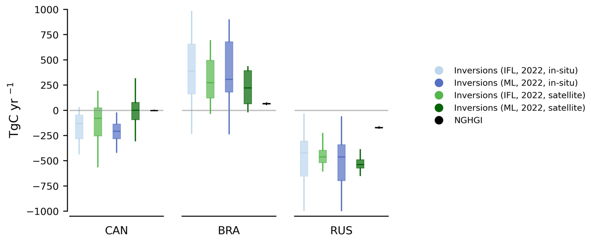
Figure 9 Net CO₂ land fluxes during the period of 2015–2020 in Canada (CAN), Brazil (BRA), and Russia (RUS). “IFL” stands for using the intact forest landscape data as a mask for non-managed land to extract land CO₂ flux from managed land, and “ML” indicates the adjusted mask used by Grassi et al. (2023) to extract land CO₂ flux from managed land. The term “in situ” indicates inversion results using in situ observations, and “satellite” represents inversions using satellite observations. Note that the inversion results here were adjusted by the lateral flux before the comparison.

6.3 Comparison of anthropogenic CH₄ emissions with Deng et al. (2022)

In our previous study, we found that satellite inversion models appear to have better agreement with NGHGIs than in situ station-based inversion models and, on the other hand, that differences between inversion models and NGHGIs in large oil- and gas-producing countries suggest an underestimation of national reports, possibly due to the omission of ultra-emitting sources by NGHGIs. With the new inversion ensemble in this study, we confirm those results (Fig. 10). In countries such as China (CHN), India (IND), and Russia (RUS), the updated inversion model set provides estimates that are closer to those of NGHGIs, but differences still exist, and the reasons for these differences are not the same. For example, differences in anthropogenic methane emissions in IND are mainly due to differences in agricultural and waste methane flux with the new inversion ensemble used in this study. In RUS, the updated inversion ensemble shows lower fossil fuel emissions, reducing the differences with NGHGIs for this sector, but higher agricultural and waste emissions than in Deng et al. (2022). Nevertheless, the updated fossil fuel emission flux is still higher than the NGHGI estimate for RUS. The remaining differences may be attributed to ultra-emitting sources or underestimated emission factors for some components of the oil and gas extraction and distribution industry in RUS. Conversely, in GULF (GULF comprises Saudi Arabia, Iraq, Kuwait, Oman, the United Arab Emirates, Bahrain, and Qatar), the new inversion model ensemble consistently reflects higher fossil fuel emission fluxes than NGHGIs, like in our previous study, and expands the difference in estimates of artificial methane flux between inversion models and NGHGIs, possibly indicating more methane leakage.

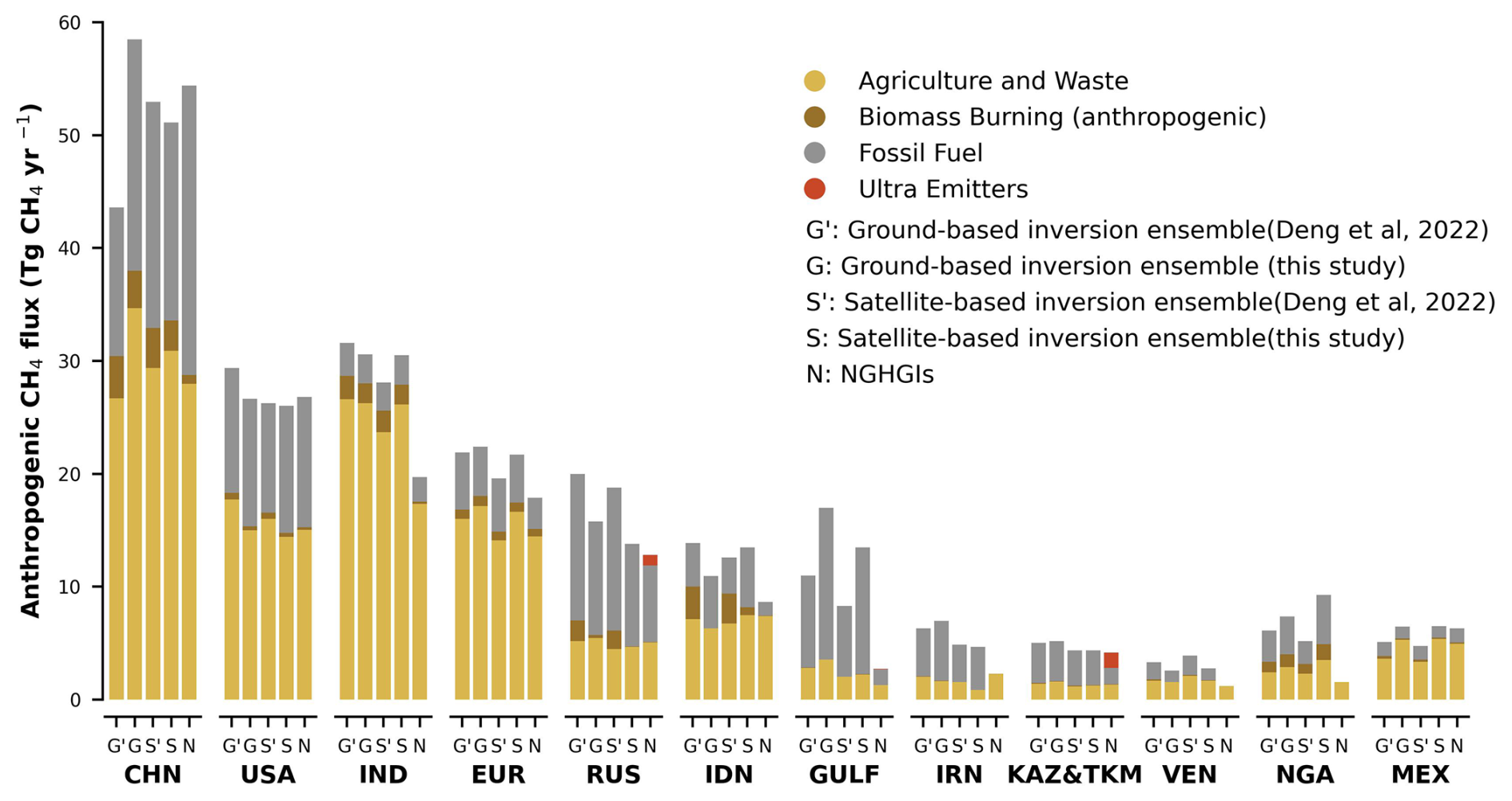
Figure 10 Annual average of anthropogenic CH₄ emissions from in situ (G) and satellite (S) inversions and national greenhouse gas inventories (N) during the period of 2010–2020. G^′ and S^′ denote the anthropogenic CH₄ flux from the in situ and satellite inversion ensembles in the previous study (Deng et al., 2022), respectively, while G and S denote the fluxes from the in situ and satellite inversion ensembles used in this study. Grey, yellow, and brown bars represent the CH₄ fluxes from the sectors of fossil fuel combustion, agriculture and waste, and biomass burning, respectively. On top of NGHGI emissions, emissions from ultra-emitters (red) are added to NGHGI estimates (diagnosed from S5P TROPOMI measurements for the period 2019–2020; Lauvaux et al., 2022).

6.4 Influence of the prior used in CH₄ inversions

The use of different priors can also influence the inversion results of the data. Figure 11 presents the sets of inversion results using EDGAR (blue) and GAINS (purple) as priors. In most countries, the median values of the two inversion result sets are similar. However, in countries such as Russia (RUS), the United States (USA), Iran (IRN), and Mexico (MEX), significant differences are observed between the two inversion result sets, which may primarily stem from the differences in the inversion results for fossil CH₄ emissions (Fig. 12). In RUS and USA, the inversion results using GAINS as priors are consistently higher than those using EDGAR as priors. In RUS, the satellite inversion results using GAINS as priors are higher by 45 % during 2010–2020, and the ground-based inversion results are higher by 75 % during 2000–2020. In the case of the USA, the inversion results using GAINS as priors exhibit a completely different trend compared to the ones obtained using NGHGIs and EDGAR as priors. The inversion results using GAINS as priors, from both satellite and ground-based measurements, show a rapid growth trend by increasing by 24 % from 2010 to 2020. In IRN and MEX, the inversion results using GAINS as priors are lower than those using EDGAR as priors. For IRN, the differences between satellite inversion results using different priors are not significant, and the trends are similar. However, the ground-based inversion results are very close between 2000–2013, but after 2013, a steep increase is observed in the ground-based inversion results using GAINS as priors. On the other hand, in MEX, the ground-based inversion results are similar, but the satellite inversion results using GAINS as priors are relatively low, by 14 % on average. Such discrepancies may arise from differences in inventory methodologies and the resulting estimations. As shown in Supplement Fig. S1 in Tibrewal et al. (2024), similar discrepancies were found between the two inventories in these countries, which report a higher estimation from GAINS in RUS and USA compared to EDGAR during 2011–2020 and a lower estimation in IRN. As noted in Tibrewal et al. (2024), EDGAR is based on various versions of national inventory reports (NIRs) that utilize different combinations of emission factors from the IPCC, while GAINS employs an independent estimation approach. This highlights the critical role of prior data selection in determining the accuracy of CH₄ emission estimates.

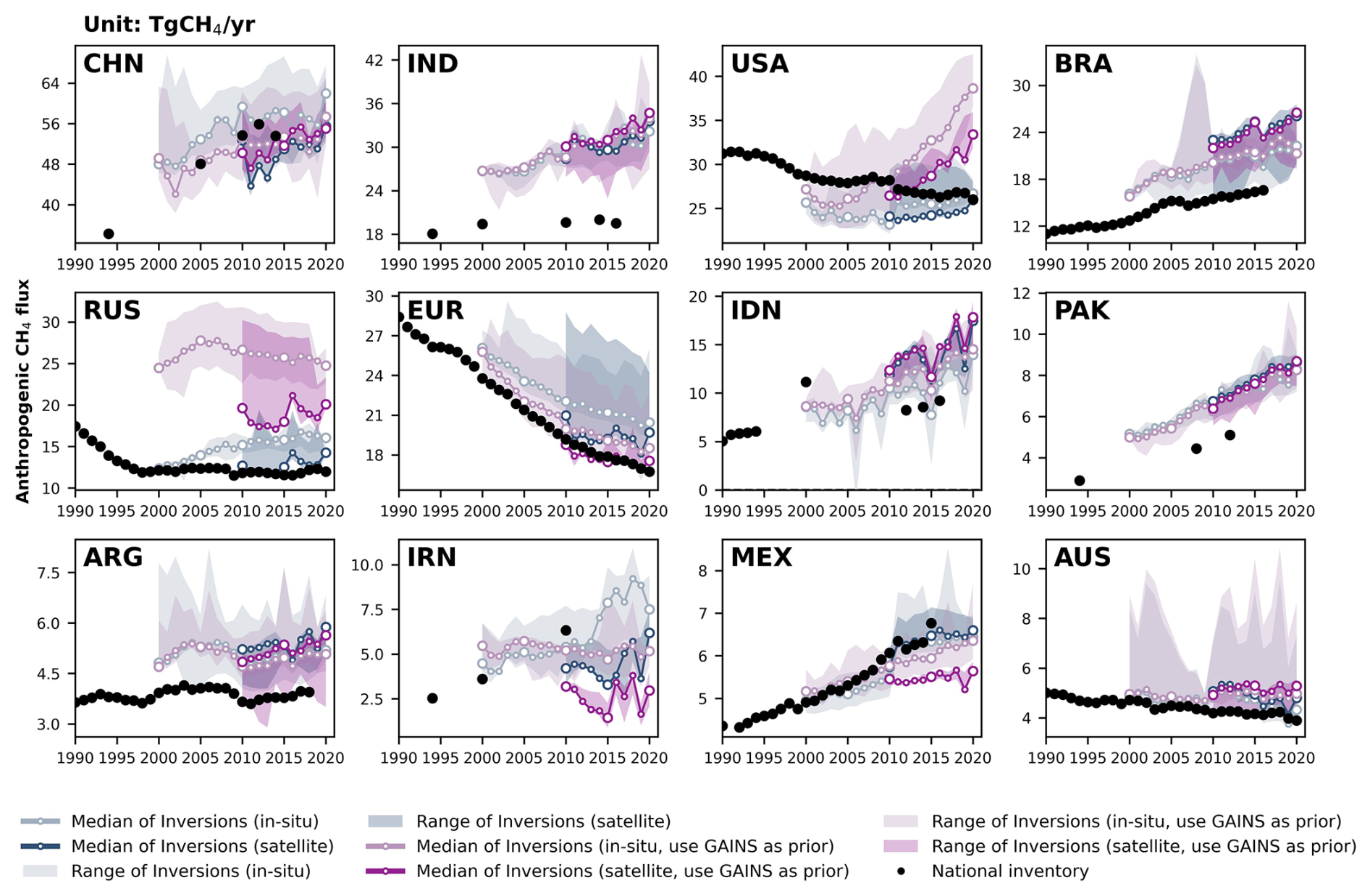
Figure 11 Total anthropogenic CH₄ fluxes for the 12 top emitters: China (CHN), India (IND), the United States (USA), Brazil (BRA), Russia (RUS), the European Union (EUR), Indonesia (IDN), Pakistan (PAK), Argentina (ARG), Iran (IRN), Mexico (MEX), and Australia (AUS). The black dots denote the reported values from NGHGIs. The light-blue lines and areas denote the median and maximum–minimum ranges of in situ CH₄ inversions based on EDGAR v6.0 as the prior, and the dark-blue ones denote those of satellite inversions, respectively. The light-purple lines and areas denote the median and maximum–minimum ranges of in situ CH₄ inversions based on GAINS (Höglund-Isaksson et al., 2020) as the prior, and the dark-purple ones denote those of satellite inversions, respectively.

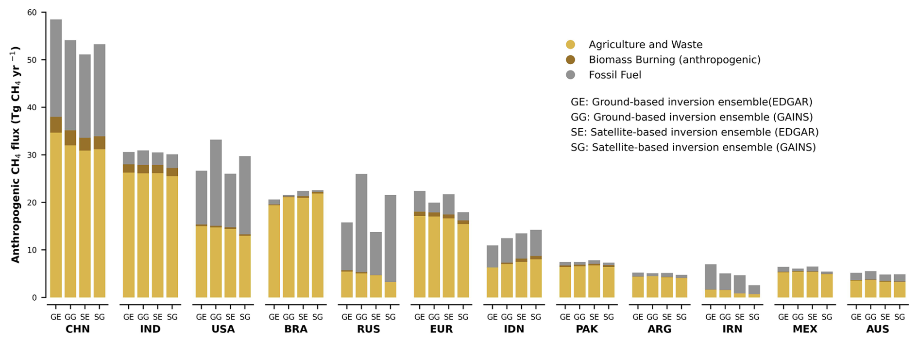
Figure 12 Annual average of anthropogenic CH₄ emissions from in situ and satellite inversions based on two different priors during the period of 2010–2020. GE and SE denote the anthropogenic CH₄ flux from the in situ and satellite inversion ensembles based on EDGAR v6.0 as the prior, while GG and SG represent the in situ and satellite CH₄ inversions based on GAINS as the prior.

6.5 Comparing anthropogenic N₂O flux with our previous study

The updated N₂O inversion results show systematically higher anthropogenic emissions than our previous N₂O inversion results (Deng et al., 2022), resulting in larger discrepancies between N₂O inversion results and NGHGIs in most countries in Fig. 13. Countries such as Brazil (BRA), the Democratic Republic of the Congo (COD), Indonesia (IDN), Colombia (COL), Sudan (SDN), Australia (AUS), and Venezuela (VEN) exhibit significant differences. These discrepancies may be attributed to the use of lower IPCC default emission factors in the national inventories of these tropical countries, leading to lower NGHGI results. The IPCC default emission factors are derived from measurements primarily conducted in temperate regions of the Northern Hemisphere (e.g., Europe and the United States (USA)), which explains the better alignment of inversion results with inventories in those regions. Notably, in the case of the USA, the median of the updated N₂O inversion results is very close to that of NGHGIs. The median of the N₂O inversion results from Deng et al. (2022) was 42 % lower than that of the NGHGIs between 2005 and 2015, whereas the median of the updated inversion models is only 4 % lower. This demonstrates improved consistency in the updated inversion system results for the USA. Additionally, in countries such as India (IND), IDN, COL, COD, Sudan (SDN), and VEN, our N₂O inversion results have a larger distribution compared to the previous study, indicating that the new N₂O inversion ensemble (n=4) has less consistency in these countries compared to the previous ensemble (n=3).

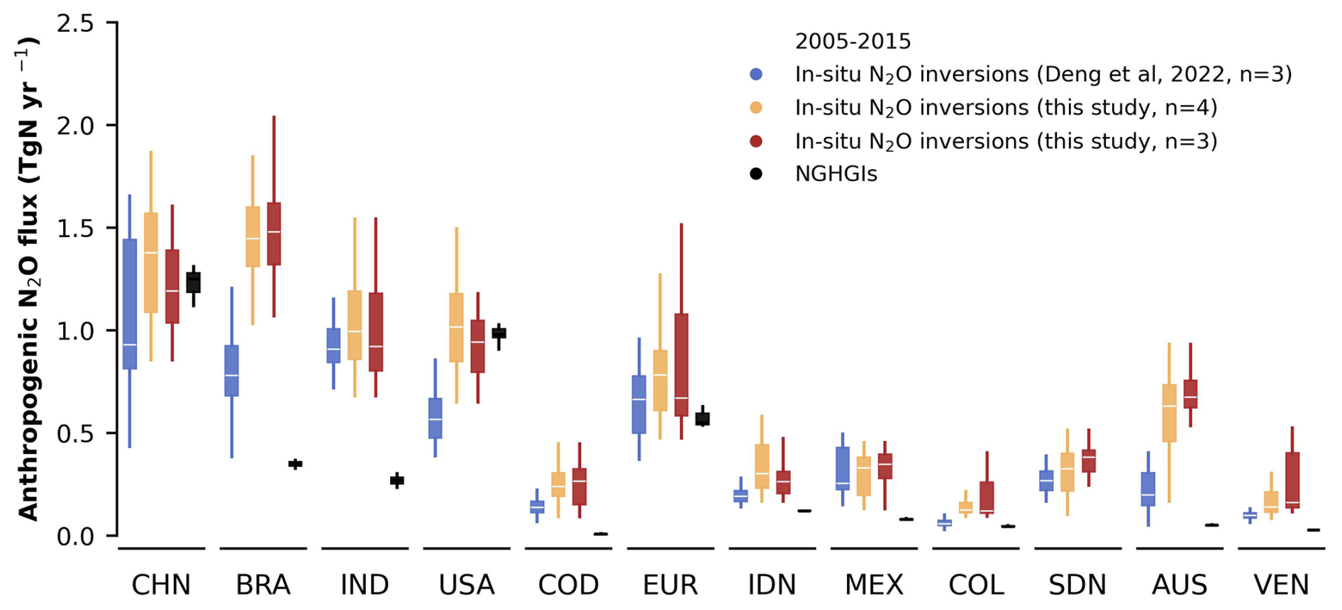
Figure 13 Anthropogenic N₂O fluxes during the period of 2005–2015 in China (CHN), Brazil (BRA), India (IND), the United States (USA), the Democratic Republic of the Congo (COD), the European Union (EUR), Indonesia (IDN), Mexico (MEX), Colombia (COL), SDN (Sudan), Australia (AUS), and Venezuela (VEN). Blue boxes denote the in situ inversion results from Deng et al. (2022) processed from the Global Carbon Budget 2020 (Friedlingstein et al., 2020). Dark-yellow boxes denote the inversion results processed in this study. Black boxes denote the NGHGI-reported values. Red boxes show results from three of the four models in this study, consistent with those in Deng et al. (2022).

7 Data availability

Processed GHG (CO₂, CH₄, and N₂O) data from inverse models and UNFCCC NGHGIs are available at https://doi.org/10.5281/zenodo.13887128 (Deng et al., 2024).

This dataset contains five data files, described as follows.

The file “Inversions_CO₂_v2022.csv” includes the NEE CO₂ flux from managed lands for the nine CO₂ inverse models. It includes eight fields: years (from 1960 to 2021), country, value (unit: Tg C yr⁻¹), sector (“land”: without the adjustment of lateral C flux; “land_cor”: with lateral C flux adjustment), source, gas, observation (“in situ”: in situ-based; “satellite”: satellite-based), and version (“CO₂_ML_v2022” only).

The file “Inversions_CH₄_v2022.csv” includes CH₄ flux from anthropogenic sources for the six CH₄ inverse models. It includes eight fields: years (from 2000 to 2020), country, value (unit: Tg CH₄ yr⁻¹), sector (“agrw”: agriculture and waste; “fos”: fossil fuel; “ant”: anthropogenic, i.e., agrw + fos), source, gas, observation (“in situ”: in situ-based; “satellite”: satellite-based), and version (“CH₄_2022_V1”: uses EDGAR as priors; “CH₄_2022_V2”: uses GAINS as priors).

The file “Inversions_N2O_v2022.csv” includes the anthropogenic N₂O flux from managed lands for the four N₂O inverse models. It includes eight fields: years (from 1995 to 2020), country, value (unit: Tg N₂O yr⁻¹), sector (“ant” only, for anthropogenic), source, gas, observation (“in situ” only, for in situ-based), and version (“N2O_ML_v2022” only).

The file “lateral_CO₂_v2022.csv” includes the national lateral C flux from rivers and trade.

The file “NGHGIs_v2022.csv” includes the national inventory data collected from UNFCCC NGHGIs (unit: Gg yr⁻¹).

8 Conclusions

This study reconciles the gap between atmospheric inversions and UNFCCC NGHGIs for each of the three greenhouse gases, based on the post-processing framework we proposed in our previous study (Deng et al., 2022). We update inversion results and NGHGI datasets to present the most up-to-date discrepancies between these two estimates. For CO₂, we updated the inversion results up to 2021; added a new inversion ensemble including inversions based on satellite observations; and applied a new mask of national managed land based on NGHGI reports in Russia, Brazil, and Canada. For CH₄, we compared NGHGIs and CH₄ inversion results up to 2020 by splitting the anthropogenic fluxes from inversions and aggregating prior estimates from each sector or by removing fluxes of natural processes, and we discussed the uncertainties related to using different priors in CH₄ inversions. For N₂O, we updated the inversion results up to 2019 and included the MIROC4-ACTM N₂O inversion and also separated the fluxes from managed land using the same method as for CO₂.

In the case of CO₂, we updated the managed-land mask for Canada, Brazil, and Russia based on maps derived from NGHGIs and adjusted tree-cover thresholds. The analysis of different managed-land mask definitions shows that the new mask, which is more consistent with the definition of managed land in the NGHGIs for these countries, improves the agreement between managed-land CO₂ fluxes and NGHGIs in Russia and Canada. However, in Brazil, the new mask increases the gap between the estimated land carbon emissions and NGHGIs. Further analysis is needed to understand the sources of and reasons for discrepancies and uncertainties between inversion estimates and NGHGIs. Thus, we still recommend that countries report their managed land in a spatially explicit manner to enable a better evaluation of national emissions reports using inversions (and other observation-based approaches), and countries should also follow the recommendations of the 2006 IPCC guidelines encouraging countries to use atmospheric data as an independent check on their national reports (IPCC, 2006, 2019). Three additional satellite-based inversion results have been introduced for comparison with the in situ inversion results and NGHGIs. In some countries, the satellite-based inversions demonstrate better consistency with NGHGIs compared to the in situ inversion models.

For CH₄, despite the large spread of inversions, both in situ and GOSAT inversions show systematic differences with NGHGIs. We also found that Kazakhstan and Turkmenistan in Central Asia and the Persian Gulf countries in the Middle East, characterized by oil- and gas-producing industries, report much lower CH₄ emissions than atmospheric inversion estimates. While in this region, there are few ground stations and inversions depend on their prior fluxes, the fact that GOSAT and in situ-based inversions point to NGHGI emissions being underestimated suggests areas for future research to constrain the emissions of these countries. We recommend developing regional campaigns (such as those performed in Alvarez et al., 2018) to refine emission factors and to track regional oil, gas, and coal basin emissions and ultra-emitter site-level emissions using new tools (such as moderate- and high-resolution satellite imagery).

For N₂O, the prevalence of large tropical natural sources, being outside the responsibility of countries if they are located on unmanaged lands, has been overlooked before. For example, nearly half of the forests in Brazil are unmanaged according to its national inventory report. We did not solve this problem but highlighted it and proposed a new method to remove natural emissions from inversion total emissions. As many non-Annex I countries, which will have to produce inventories for the global stocktake, are tropical countries with a very active nitrogen cycle and large natural N₂O emissions, decoupling will exist between targeted emissions reductions and the observed growth rate of N₂O; this may hamper the eventual effectiveness of mitigation policies that are directly reflected in the UNFCCC NGHGI reports, especially for this greenhouse gas. It is fair to say that the uncertainty from the spread of different inversions is large enough that inversions cannot “falsify” N₂O NGHGIs in most instances. Nevertheless, for CH₄ in countries around the Persian Gulf and Central Asia, and to some extent in Russia, and for N₂O in tropical countries, Mexico, and Australia, we found that NGHGI emissions are significantly lower than inversions, which suggests that activity data or emission factors may need to be re-evaluated. Despite their large spread, inversions have the advantage of providing fluxes that are consistent with the accurately observed growth rates of each greenhouse gas in the atmosphere. The uncertainty in inversions is mainly a systematic bias due to internal settings or to the choice of a transport model. It does not mean that inversions cannot be used for monitoring interannual variability and trends in fluxes in response to mitigation efforts, since most of their bias should have a small temporal component.

The study of global inversions at the country scale rather than at the traditional subcontinent scale (e.g., the “TransCom3 regions” of Gurney et al., 2002) obviously pushes inversions close to the limit of their domain of validity, even in the case of large countries. The densification of observation networks and systems, especially from space, increases the observational information available at all spatial scales and gradually makes it possible to study smaller countries and reduce uncertainties in inversion results. This densification must be accompanied by a corresponding increase in the horizontal resolution of inversion systems (both the transport model and the control vector to be optimized). Note that the spatial resolution of most inverse models such as those contributing to the global carbon–methane–nitrous oxide budget is larger than 1° (see Table A4 in Friedlingstein et al., 2022; Table S6 in Saunois et al., 2020; and Table 1 in Tian et al., 2024). They will likely soon have to go below 1° on a global scale to remain competitive for this type of study, despite the high computational challenge posed by the atmospheric inversion of long-lived tracers.