Aboveground biomass dataset from SMOS L-band vegetation optical depth and reference maps

Aboveground biomass (AGB) is an essential component of the Earth's carbon cycle. Yet, large uncertainties remain in its spatial distribution and temporal evolution. Satellite remote sensing can help improve the accuracy of AGB estimates. In particular, the L-band (1.41 GHz) vegetation optical depth (VOD) derived from the SMOS (Soil Moisture and Ocean Salinity) mission is a good AGB proxy. Averaging the SMOS L-VOD over a year and linking it to an existing AGB map constitute a well-established method to derive a spatial relationship between the two quantities. Then, a temporal extrapolation of this spatial relation derives global and harmonized AGB time series from the L-VOD. This study refines this protocol by analyzing the impact of three factors on the AGB–VOD calibration. First, an analysis shows that ascending and descending VOD can be properly merged to estimate the AGB. Second, the use of a single global spatial relationship is preferred over several regional ones. Third, this new AGB dataset is compared with other published AGB datasets to assess the validity of the temporal extrapolation. The produced dataset provides vegetation biomass values up to 300 Mg ha⁻¹ from 2011 onward. It shows more interannual variability than the other available time series and presents globally lower AGB estimates. In general, the resulting AGB is consistent with the AGB maps of the Climate Change Initiative (CCI) Biomass version 5 (average Pearson's correlation coefficient 0.87) and can be used in AGB studies. The AGB dataset has been produced from the Level 2 SMOS products with one global VOD–AGB relationship, mixing ascending and descending orbits. The AGB dataset, including the spatial bias, is open-access and the NetCDF files are available at https://doi.org/10.12770/95f76ff0-5d89-430d-80db-95fbdd77f543 (Boitard et al., 2024).

1 Introduction

In the context of climate change and global warming caused by anthropogenic activities, understanding, monitoring, and managing the Earth's carbon cycle are critical (Grace, 2004). Vegetation biomass plays a key role in this cycle (Hese et al., 2005; Houghton, 2005; Houghton et al., 2009). In particular, the forest carbon biomass constitutes a large carbon reservoir as it contains most of the carbon stored in the vegetation (Pan et al., 2013). Up to date the world's forests are a global carbon sink (Pan et al., 2011). Yet locally, they can act as either major sinks or prominent sources of atmospheric carbon dioxide (CO₂) depending on land use practices, meteorological conditions, and natural and anthropogenic wildfires (Clark, 2004; Wear and Coulston, 2015; Wigneron et al., 2020). Globally, the ability of forests to absorb carbon under a changing climate remains poorly known (Luyssaert et al., 2007). The total aboveground biomass (AGB, which accounts for the entire land vegetation biomass) is strongly linked to the carbon content in the vegetation (Losi et al., 2003; Djomo et al., 2011). Hence, mapping this essential climate variable and following its evolution in space and time are fundamental for precise and reliable monitoring of the Earth's carbon balance.

Estimating the AGB from the ground is challenging, as densely vegetated areas are often remote (tropical and boreal forests) and hard to navigate through. In situ measurements are by definition local, and global monitoring would involve the installation and maintenance of a dense network of stations or multiple and frequent in situ measuring campaigns.

This is why deriving AGB from satellite remote sensing, which provides global and regular coverage of the Earth's surface, complements AGB in situ data very well. Optical indices have been used for decades to monitor terrestrial vegetation at medium and high resolutions (Zeng et al., 2022; Lu, 2006). Yet, such observations cannot be relied on to estimate the AGB globally. They are mainly sensitive to the green component of the top canopy layer (Purevdorj et al., 1998) and tend to saturate over densely vegetated areas (Baret and Guyot, 1991). They are also heavily affected by atmospheric conditions such as clouds, aerosols, or haze (Lu et al., 2017), which are common in moist tropical areas. For this reason, spaceborne synthetic aperture radars (SARs), with their all-weather capabilities, have proved useful to AGB estimation. Numerous studies, both theoretical and experimental, have demonstrated that SAR data respond to forest AGB up to a certain saturation point (Mitchard et al., 2009; Le Toan et al., 2011; Yu and Saatchi, 2016; Cartus and Santoro, 2019). This saturation point increases with wavelength (i.e., the P- and L-band are more sensitive to AGB than the C- and X-band). Beyond this level, the sensitivity diminishes. Interestingly, in the case of dense forests, there might be a negative correlation observed between L-band backscatter and high AGB values (Mermoz et al., 2015).

More recently, the data acquired by spaceborne passive microwave radiometers at L-band have received great attention for AGB estimation and related applications. These instruments deliver information complementary to optical indices and radar acquisitions. Despite their coarse spatial resolution (approximately 40 km), they benefit from a low emission contribution of the atmosphere. They can measure the microwave radiation emitted by the Earth's surface in all weather and light conditions. The Soil Moisture and Ocean Salinity (SMOS) mission (Kerr et al., 2010) was launched in November 2009. Over land, the SMOS passive microwave radiometer at L-band is used to retrieve the surface soil moisture (SM) along with a vegetation optical depth (VOD). This radiative parameter is also derived at L-band from the Soil Moisture Active Passive (SMAP) mission (Entekhabi et al., 2010; Konings et al., 2017; Chaubell et al., 2021). This L-band VOD (or L-VOD; Wigneron et al., 2007) characterizes how much the surface signal is attenuated by the vegetation, as well as the vegetation's own emission. It is then defined as an optical depth. Theory and previous works (Jackson and Schmugge, 1991; Grant et al., 2012) showed that the L-band VOD is strongly influenced by the vegetation water content (VWC). In addition, it is highly sensitive to AGB (Rodríguez-Fernández et al., 2018; Mialon et al., 2020; Frappart et al., 2020; Vittucci et al., 2019) and does not saturate as much as higher-frequency-band VOD (C, X, or Ka) over dense forests (Rodríguez-Fernández et al., 2018; Chaparro et al., 2019; Wang et al., 2021). Consequently, as recently confirmed by Dou et al. (2023), the L-VOD is a good AGB proxy when averaged over a long enough time period. This time period typically covers a year to iron out the effects on L-VOD of diurnal and seasonal variations of the water content in the vegetation.

However, up to date, there is no equation or model to directly compute the AGB from L-band acquisitions without using pre-existing AGB maps. Liu et al. (2015), Rodríguez-Fernández et al. (2018), Mialon et al. (2020), and Wigneron et al. (2020) used several static AGB maps to derive spatial relationships between VOD datasets and reference AGB estimates, while Prigent and Jimenez (2021) and Salazar-Neira et al. (2023) directly established a link between these static AGB maps and L-band brightness temperatures using neural networks. These static AGB maps have high spatial resolutions compared to SMOS, ranging from 100 m (Santoro and Cartus, 2024) to 1000 m (Avitabile et al., 2016), but are restrained to a year or a couple of years of reference. These maps may also present large discrepancies and uncertainties (Mitchard et al., 2013).

To retrieve harmonized AGB time series from the L-VOD, the published literature focuses on establishing a spatial relationship that is later extrapolated over time. This study capitalizes on the same method as already described in Rodríguez-Fernández et al. (2018) and Mialon et al. (2020) and goes further by evaluating the impact of three factors on the SMOS L-VOD–AGB calibration. The work carefully investigates the influence of mixing morning and afternoon overpasses to maximize the number of observations per node, calibrating a single global relationship or several local relationships, and extrapolating a spatial relationship over time. Importantly, the derived AGB is provided with its associated error. The new AGB dataset is estimated from 12 years of SMOS L-VOD and is freely accessible from the SMOS French ground segment, CATDS (Centre Aval de Traitement des Données SMOS).

Hereafter, Sect. 2 introduces the SMOS L-VOD products and the AGB reference maps. Section 3 describes the methodology. Section 4 presents the obtained results and a temporal analysis, further discussed in Sect. 5. Finally, the conclusions are summarized in Sect. 7.

2 Data

This section presents the SMOS products used to estimate the AGB and the existing AGB maps that are used to either perform the AGB estimates or evaluate the results.

2.1 SMOS products

SMOS (Kerr et al., 2010) is an Earth observation mission managed by the European Space Agency (ESA) and the Centre National d'Études Spatiales (CNES). This satellite, launched in November 2009, measures the Earth's thermal emission as brightness temperatures (TBs) at a frequency of 1.41 GHz in full polarization, i.e., four Stokes parameters, for a broad range of incidence angles (angles from 0 to 55° are used for the SM–VOD retrievals). SMOS crosses the Equator at 06:00 (18:00 LT) for ascending (descending) orbits.

The SMOS Level 2 (L2) products (Kerr et al., 2012) from version 700 between 2011 and 2023 are used for this study. The year 2010 is set aside for two reasons. The first 5 months (January–May) were dedicated to the commissioning phase, during which the instrument was stabilizing and extensive tests and calibration were performed. This year was also extremely polluted with radio frequency interferences (RFIs). These RFIs are emitted by human-built equipment and mask the Earth's natural emission over large areas. They prevent SMOS from globally covering the Earth (Oliva et al., 2016). The core processing L2 algorithm is based on the L-MEB radiative model (Wigneron et al., 2007), which uses the τ–ω model (Mo et al., 1982) to account for the vegetation layer. In summary, on appropriate pixels, an initial couple (SM, VOD) is fed to a forward model computing the corresponding theoretical TB at all incidence angles and for both horizontal and vertical polarizations. The value of the (SM, VOD) couple is iteratively modified. The iteration process stops when the cost function derived from the sum of the squared weighted differences between the modeled and measured TB reaches a minimum. The value of (SM, VOD) which minimizes the cost function is written out to the output product. The quality of the retrieval is evaluated by two variables reported in the L2 data. The first is the probability of Chi2 (Chi2_P field in the product) that measures how close the modeled TBs are to the SMOS TB. The Chi2_P parameter ranges from 0 (poor quality) to 1 (excellent quality). The second one is the quality index labeled as VOD_DQX. It translates how the radiometric TB noise propagates through the retrieval model, and constitutes the lower bound of the uncertainty. It ranges from [0.02–0.06] for VOD between 0 and 0.6 to [0.2–0.25] for VOD higher than 1.2. Another point worth mentioning is that the L2 algorithm does not output VOD for footprints with little to no vegetation such as the Saharan desert, Antarctica, or any wet surfaces with no vegetation reported in the auxiliary datasets.

ESA freely distributes the L2 products (ESA, 2021) in a binary format. The data are provided on an icosahedral Snyder equal-area (ISEA) 4H9 grid (Sahr et al., 2003) in swath mode with an almost constant inter grid point distance of 15 km. Considering the L2 file format and spatial projection, the products are pre-processed to work with common temporal and spatial grids for all input files. The SMOS orbit files are aggregated into daily ascending and descending maps. Where multiple measurements were acquired the same day, the data with the highest quality and closest to the sub-track are selected. These cases are mainly located in the high (>60° N) latitudes. Finally, the variables are reprojected to the Equal-Area Scalable Earth Grid (EASE grid) version 2.0 (Brodzik et al., 2012, 2014) global equal-area projection (EPSG: 6933), with a grid sampling of 25 km at 30° of latitude. The resampling is performed through a Delaunay triangle interpolation if possible (three valid interpolants exist) or linear if only two valid interpolants are available. The EASE 2 grid offers the advantage of being regular and is the default spatial projection for the SMOS CATDS ground segment products such as Level 3 (L3; Al Bitar et al., 2017). An example of the 2018 averaged L2 v700 VOD values resampled to the EASE 2 grid at 25 km mixing ascending and descending orbits (AD) is displayed in Fig. 1.

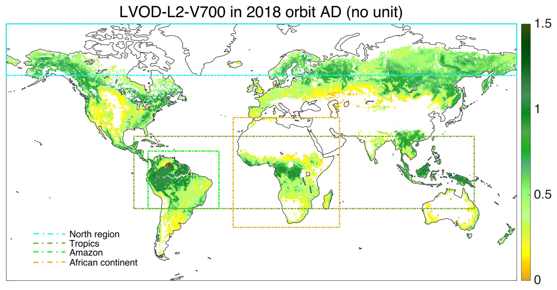
Figure 1 L-VOD from SMOS L2 v700 products averaged over 2018. Ascending and descending orbits are mixed. Values where RFI contamination is higher than 20 %, where the Chi2_P is lower than 5 %, or where the air temperature is below 0  °C are filtered out. Pixels with an AGB reference value equal to 0 are also filtered out, and outliers are discarded. The colored rectangles show the extent of the different regions (see Sect. 3.1 for more details about the regions) considered in the study.

2.2 Aboveground biomass reference maps

This study involves the three AGB reference maps described below. The AGB maps from the ESA Climate Change Initiative (CCI) (Santoro and Cartus, 2024) and Avitabile et al. (2016) were used as calibration data for the production of the SMOS-based AGB maps. The yearly AGB maps from Xu et al. (2021a), covering the years 2000–2019, were used to compare and contextualize the AGB time series resulting from this work. The AGB reference maps were regridded from their native sampling to the same EASE grid version 2 (25 km) as the interpolated L2 products. The regridding method was a weighted average of all meaningful (“non-no-data”) pixels.

2.2.1 ESA Biomass CCI 2015–2021 global AGB map

The ESA Climate Change Initiative (CCI) Biomass maps (Santoro and Cartus, 2024) are outputs of the ESA CCI Biomass project. The AGB estimation was derived using the radar backscatter intensity data captured by the Phased Array-type L-band Synthetic Aperture Radar (PALSAR2) on the Advanced Land Observing Satellite (ALOS2) and the Sentinel-1 satellites. The process of AGB estimation was also based on lidar metrics and surface reflectances. The AGB map is updated annually with a pixel size of 100×100 m. Each CCI AGB map comes with its associated standard deviation, which is a combination of the standard deviations from the input data, the modeling algorithms, and the merging procedure. Version 5.01 (v5) of the maps is used for this work. Global maps for the years 2010 and 2015–2021 are distributed at several ground resolutions (100 m, 1, 10, 25, and 50 km). The aggregated resolution at 25 km is used for the study and reprojected onto the EASE 2 grid (equal-area, 25 km at 30° of latitude). The standard deviation of the aggregated maps at 25 km is significantly lower than the standard deviation of the original-resolution (100 m) maps and lies below 15 % of the AGB value for most pixels. The mean uncertainty ranges from 1 Mg ha⁻¹ for AGB values below 50 to 25 Mg ha⁻¹ for AGB values above 250 Mg ha⁻¹. Figure 2a shows the distribution of AGB on Earth in 2018 according to Santoro and Cartus (2024).

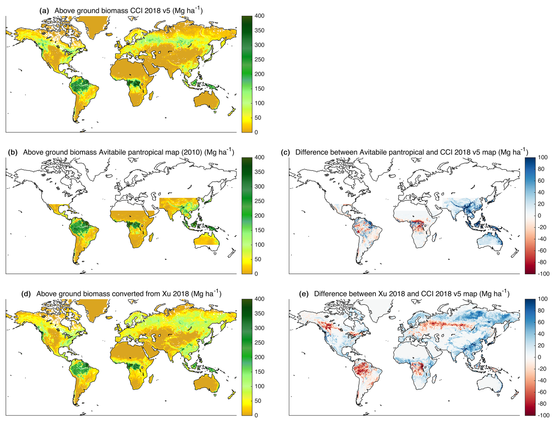
Figure 2 The reference maps used in this study and the spatial differences between them. (a) Aboveground biomass from CCI 2018 v5 (Santoro and Cartus, 2024), (b) aboveground biomass from Avitabile et al. (2016), (c) aboveground biomass difference for Avitabile et al. (2016) minus CCI 2018 v5, (d) aboveground biomass in 2018 converted from Xu et al. (2021b), and (e) aboveground biomass difference for Xu et al. (2021b) minus CCI 2018 v5. All units are in Mg ha⁻¹ and all maps are resampled to the EASE 2 grid at 25 km.

2.2.2 Avitabile 2010 pantropical AGB map

The 1 km pixel size AGB map from Avitabile et al. (2016), limited to the pantropical region, was produced by integrating two pre-existing AGB maps from Saatchi et al. (2011) and Baccini et al. (2012) for the year 2010. This integration was achieved by employing an independent set of field observations and regionally adjusted high-resolution biomass maps, which were then standardized and aggregated to produce almost 15 000 AGB reference data points at a 1 km scale. The data fusion approach, involving bias correction and a weighted linear averaging technique, was implemented separately within distinct zones characterized by uniform error profiles in the Saatchi et al. (2011) and Baccini et al. (2012) AGB maps. The map from Avitabile et al. (2016), resampled onto the EASE grid 2 at 25 km, is shown in Fig. 2b. Figure 2c exhibits the differences of the AGB from Avitabile minus the one from CCI 2018 v5.

2.2.3 Xu 2000–2019 global AGB maps

Xu et al. (2021b) calculated the live (aboveground and belowground) carbon biomass of global terrestrial ecosystems on an annual basis, covering the years 2000 to 2019. Reference data, including 100 000 plots coupled with airborne lidar data covering more than 1 Mha of tropical forests globally and satellite lidar survey detailing the height structure of global vegetation across over 8 million sample footprints, were used to feed a machine learning model. Reference data were converted into estimates of both aboveground and belowground biomass (BGB) using established allometric models and the root-to-shoot ratio. These data are used as training data for the machine learning algorithm, together with microwave and optical satellite imagery collected from 2000 to 2019. The annual carbon density maps of live woody vegetation are distributed in Xu et al. (2021a). For this study, the live carbon density maps were converted to aboveground carbon density thanks to the root-to-shoot ratio list provided in the supplementary material of Xu et al. (2021b). This aboveground carbon density is then converted to AGB by dividing the carbon density by 0.49 (Xu et al., 2021b). The Xu converted AGB map for 2018 reprojected to the EASE 2 grid at 25 km appears in Fig. 2d. Figure 2e shows the difference of the AGB from Xu minus the AGB from CCI v5 for the year 2018.

3 Methods

3.1 Converting VOD to AGB

The methodology used to derive the AGB is detailed in Fig. 3. It exhibits the input and output datasets and the setup. The purpose of this workflow is to calibrate a relationship between the L-VOD and the AGB and quantify the impact of three factors on the calibration. The first factor is the relevance of merging the SMOS overpasses with different local time. SMOS has a polar sun-synchronous orbit. During the ascending orbits (around 06:00 LT), thermal equilibrium is reached and the vegetation temperature is supposed to be close to the air temperature at 2 m height (Kerr et al., 2012). This hypothesis is not valid for descending orbits (18:00 LT) and may lead to a larger uncertainty in the VOD retrievals. Nevertheless, descending orbits help fill the spatial gap in areas strongly affected by RFI. If both orbit types can be merged properly without impacting the quality of the calibration, the spatial extent of the AGB estimations will be increased. The second factor is the impact of calibrating one global relationship versus several regional ones. The regions considered in this study appear in colored rectangles in Fig. 1: the Amazon (25° S–15° N and 80–30° W), the tropics (25° S–25° N and 90° W–150° E), the African continent (37° S–37° N and 20° W–55° E), and the north region (50–90° N). The third and last factor to be tested is the relevance of extrapolating a spatial relationship over time.

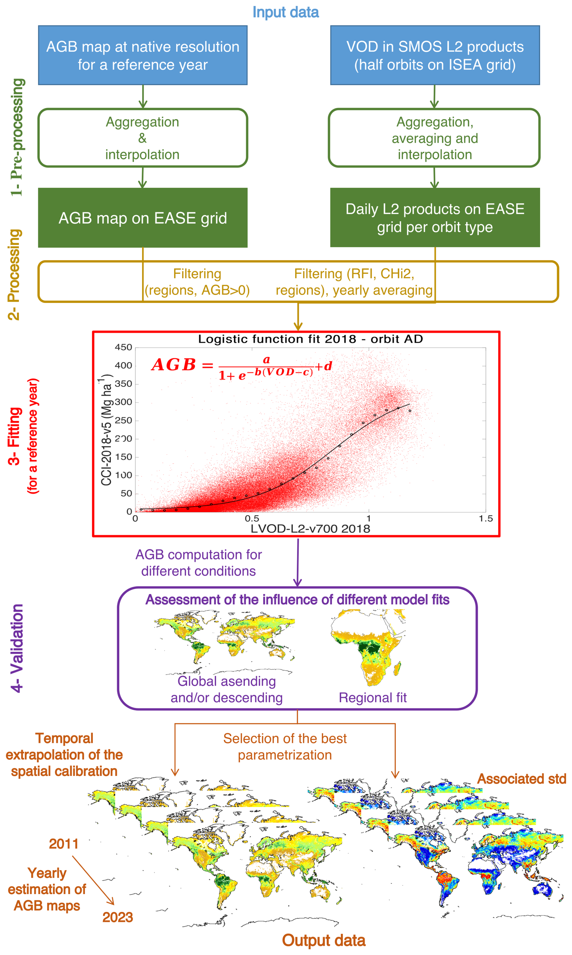
Figure 3 Overview of the methodology for estimating yearly AGB maps from the SMOS L-VOD and an AGB reference map.

For conciseness, this paper describes the methodology and results with the ESA CCI Biomass 2018 map (CCI 2018; Santoro and Cartus, 2024) as the calibration dataset. Therefore, the relationship between these AGB reference values and the SMOS VOD estimates acquired the same year (2018) is described and discussed. Once the spatial calibration of the AGB–LVOD relationship is thoroughly studied for the reference year, it is extrapolated over time to all other SMOS years. The same procedure is repeated to create AGB time series estimates from other AGB reference maps. For now, the only other AGB reference map used in this study is the one from Avitabile et al. (2016), representative of the year 2010. This map is hence linked to SMOS L-VOD from 2011 as 2010 does not meet the quality requirements (see Sect. 2). Ultimately, there are as many AGB time series estimates as reference maps used. Currently, there is one NetCDF file holding the AGB time series estimates from the CCI reference map and one NetCDF file holding the AGB time series estimates from the Avitabile et al. (2016) reference map. Xu et al. (2021b) maps are only used for comparison.

The workflow is divided into four steps numbered 1 to 4 in Fig. 3. During step 1 (pre-processing), the SMOS products and AGB calibration maps are aggregated, resampled, and averaged for the common period (here 2018 for CCI used as the reference) as described in Sect. 2. The L-VOD was aggregated for ascending and descending orbits separately to investigate the influence of the orbit local time on the calibration.

In step 2 (processing) the SMOS L-VOD daily measurements are masked, filtered, and temporally averaged. Only pixels over continental surfaces are considered, as provided in the 1 km USGS (US Geological Survey) land–sea mask aggregated into the EASE 2 grid. Low-quality VODs are removed based on the Chi2_P and the level of radio frequency interferences (RFIs). The daily SMOS observations with more than 20 % of SMOS TBs contaminated by RFI or where Chi2_P is lower than 0.05 are filtered out. The VOD temporal series of each pixel are also checked for potential outliers: the values outside an interval of 2 standard deviations around the yearly average are discarded. Moreover, if the median value of the RFI probability over the year is greater than 20 %, the pixel is dropped for that year. If after this filtering, fewer than 10 measures remain, the pixel is also discarded. The time series are also checked for spurious discontinuities that are not induced by VOD or biomass changes. A small region of 85 EASE 2 grid pixels in the northeastern part of the Amazon rainforest requires a particular filtering. Over this area, identified in red in Fig. 1, the VOD times series experience a sudden jump in May 2015. This artifact is due to the 41r1 cycle update of the European Centre for Medium-Range Weather Forecasts (ECMWF) surface model, which led to a discontinuity in the skin temperature, as used in SMOS auxiliary files (Kerr et al., 2012). This region is masked out for the analysis conducted in this study. No other affected areas have been identified.

After cleaning, the VOD time series are then temporally averaged on a yearly basis. This step is mandatory to iron out the effects on L-VOD of the diurnal and seasonal variations of the vegetation water content. At this stage, footprints with an AGB reference value equal to 0 are discarded, as they are not useful to the AGB estimation. The region mask is also applied to quantify the impact of calibrating several local relations versus one global relation. Figure 1 shows an example L2 VOD over the full globe for the year 2018 after the processing described above.

In step 3 (fitting in Fig. 3), the AGB reference map is then compared pixel-wise against the annual SMOS L-VOD map (red points in the fitting part of Fig. 3) for the same year (for example, SMOS L-VOD in 2018 against ESA Biomass CCI AGB map for the year 2018) to check the relevance of a logistic relationship. Following the methodology described in Rodríguez-Fernández et al. (2018), the annual L-VOD is binned into 0.05-width bins. In each bin, the mean AGB from the reference map is computed (black points in the fitting part of Fig. 3) and the set of parameters of the logistic function that best fits the mean AGB–L-VOD distribution is estimated. This logistic function is defined in Eq. (1):

$$\begin{array}{}\text{(1)}& \mathrm{AGB}={\displaystyle \frac{a}{\mathrm{1}+e^{-b(\mathrm{VOD}-c)}}}+d,\end{array}$$

where a, b, c, and d are the free parameters. In Eq. (1), AGB is in Mg ha⁻¹ and the L-VOD is dimensionless. Hence a and d are in Mg ha⁻¹ and b and c have no dimension. The optimized logistic relationship is applied to the configured (particular orbit, regional or global coverage) VOD to produce AGB estimates.

3.2 Uncertainty estimation

In step 3, the reliability of the AGB estimation is also computed. Two quantifiable uncertainty sources were identified: (i) the uncertainties associated with the input data that are propagated through the process and (ii) the bias resulting from the logistic fit between the AGB and the SMOS VOD.

For (i), the Monte Carlo method is used to propagate the standard deviation of the reference AGB (available for the CCI but not for the other calibration maps). The CCI uncertainty (standard deviation) aggregated maps at 25 km from Santoro and Cartus (2024) were resampled to the EASE 2 grid. A dataset of N=10 000 reference AGB maps is created. For each pixel, the AGB value is extracted from the Gaussian distribution characterized by its mean being the reference AGB from the CCI and its standard deviation being the CCI uncertainty. From these N reference AGB maps, N logistic fits and N AGB estimations are performed. The standard deviation of the N estimated AGB can then be computed per pixel. The same Monte Carlo method is applied to propagate the uncertainty associated with the yearly averaged VOD. For each footprint, the yearly VOD_DQX is obtained through the quadratic mean of the daily VOD_DQX. This value is further divided by the square root of the number of observations, as the input TB radiometric noises are considered independent from one day to the other. The yearly VOD and associated yearly VOD_DQX are then used to create the dataset of N VOD maps.

For (ii), the dispersion (SD) of the estimated AGB for the reference year is derived against the input AGB values. The estimated AGB for the reference year is binned into 10 Mg ha⁻¹ bins. The mean of the input AGB values is computed within each bin (blue points in Fig. 4). The scattering of the estimated AGB values with respect to the input AGB map is computed per bin as half of the gap between the 84th and 16th percentiles of the differences between the reference and estimated AGB. The result is a discrete spatial bias distribution of approximately 30 values (blue bars in Fig. 4). This distribution is propagated to other years. For each year, the bias map is built by dispatching to all pixels the reference bias value of the bin into which their estimated AGB values fall (see Fig. 4).

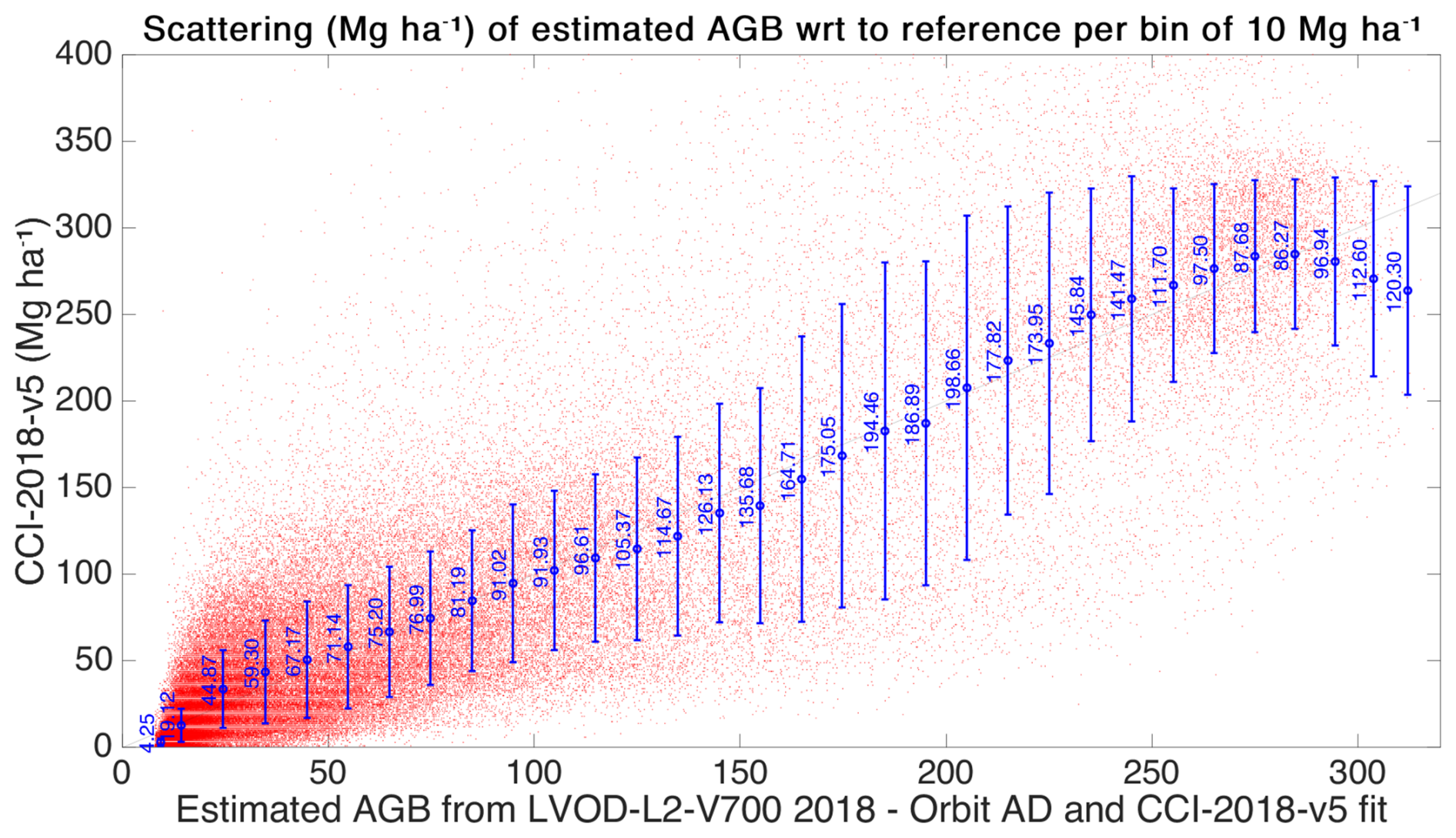
Figure 4 Computation of the SD (blue vertical bars) of the differences between estimated AGB and reference AGB in 10 Mg ha⁻¹ bins (blue dots).

3.3 AGB estimate evaluation

Finally, in step 4 (validation in Fig. 3), the resulting AGB is evaluated against the calibration data. The AGB estimations are compared to the calibration values through three classical indicators: the Pearson's correlation coefficient (R), the unbiased root mean square difference (ubRMSD), and the mean difference (bias). These statistics, complemented with maps and time series comparisons, lead to the selection of one optimal parameterization. This optimal spatial relationship is propagated to other annual VOD. The result is the AGB time series estimation for all SMOS years from a reference map (output data at the bottom of Fig. 3).

4 Results

This section presents the analysis of steps 3 and 4 from Fig. 3. In particular, it details the evaluation of the impact of the methods in terms of spatial and temporal scales. The derived AGB values are then compared against the existing dataset to assess their uncertainty.

4.1 Converting VOD to AGB

4.1.1 Relationship calibration

Prior to any AGB estimation, the calibration function between the L-VOD and the AGB is estimated. This calibration function (step 3 of Fig. 3) is presented in Fig. 5. The left panel displays the logistic function fit between the 2018 L-VOD average and the CCI 2018 for all pixels, mixing ascending and descending orbits. The right panel maps the AGB estimated from the 2018 averaged L-VOD and the calibrated logistic function. The estimated AGB reaches a maximum of approximately 300 Mg ha⁻¹ over the tropical forests (Amazonia, Congo, Philippines). Boreal forests, in the northern high latitudes, present AGB estimates around 100–150 Mg ha⁻¹. Temperate and arid regions show an estimated AGB lower than 50 Mg ha⁻¹. The spatial distribution is coherent with the CCI 2018 (see Fig. 2) and with the input L-VOD (see Fig. 1). The Sahara does not present any AGB estimate as no L-VOD retrieval is performed over this region for the L2 product. The Middle East and central Asia are masked out because of high RFI contamination and null AGB calibration data. The white areas in central Australia, southwestern Africa, southwestern America, northern Russia, northern Canada, and the central United States are caused by the filtering of the AGB reference values set to 0.

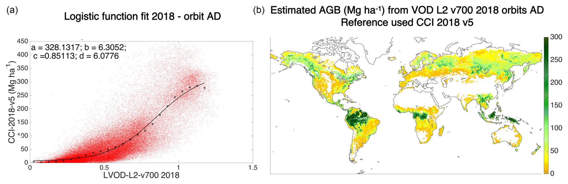
Figure 5 The left panel shows the parameter values and the mean logistic fit between the CCI 2018 v5 map and the VOD from SMOS L2 products filtered and averaged over 2018. The right panel is the estimated AGB in Mg ha⁻¹ by applying the logistic function with the estimated a, b, c, and d parameters to the 2018 averaged VOD.

The following sections detail the comparison of similar regressions conducted under the different parameterizations described in Sect. 3.

4.1.2 Relevance of merging ascending and descending orbits

Considering ascending and descending orbits separately or together gives very close calibrations of the parameters in Eq. (1), as reported in Fig. 6. Most importantly, the estimated AGB values with three orbital aggregations have similar performances in terms of bias, R, and ubRMSD compared to the CCI 2018 (Table 1).

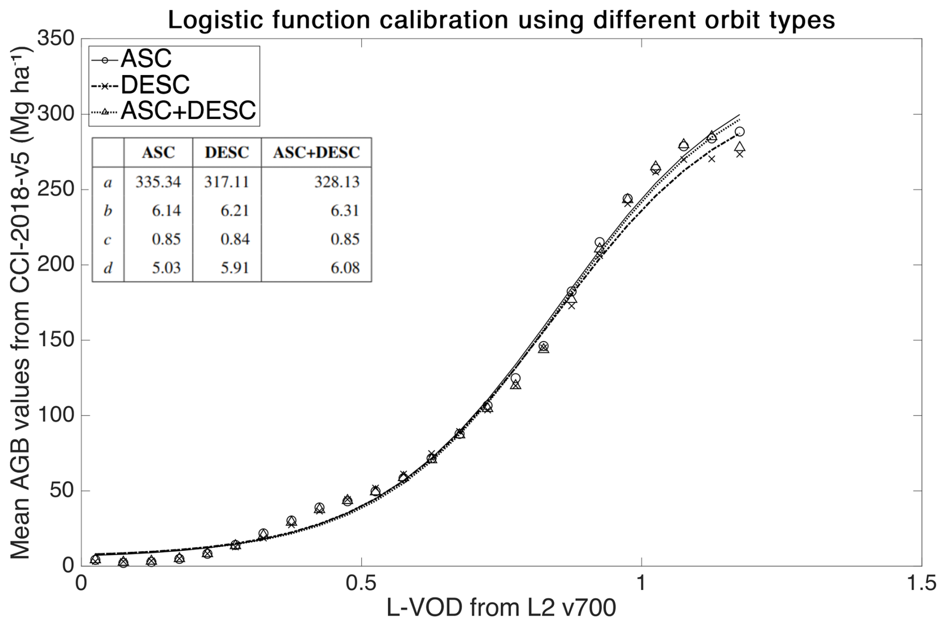
Figure 6 Logistic function fit calibrated with AGB from the CCI 2018 (Mg ha⁻¹) and the L-VOD averaged over 2018 using ascending (ASC) and descending (DESC) orbits separately or together. The table gathers the parameter values for the three logistic fits.

Table 1 R, bias (Mg ha⁻¹), and ubRMSD (Mg ha⁻¹) of the AGB estimated with the VOD from different orbit types with respect to CCI 2018.

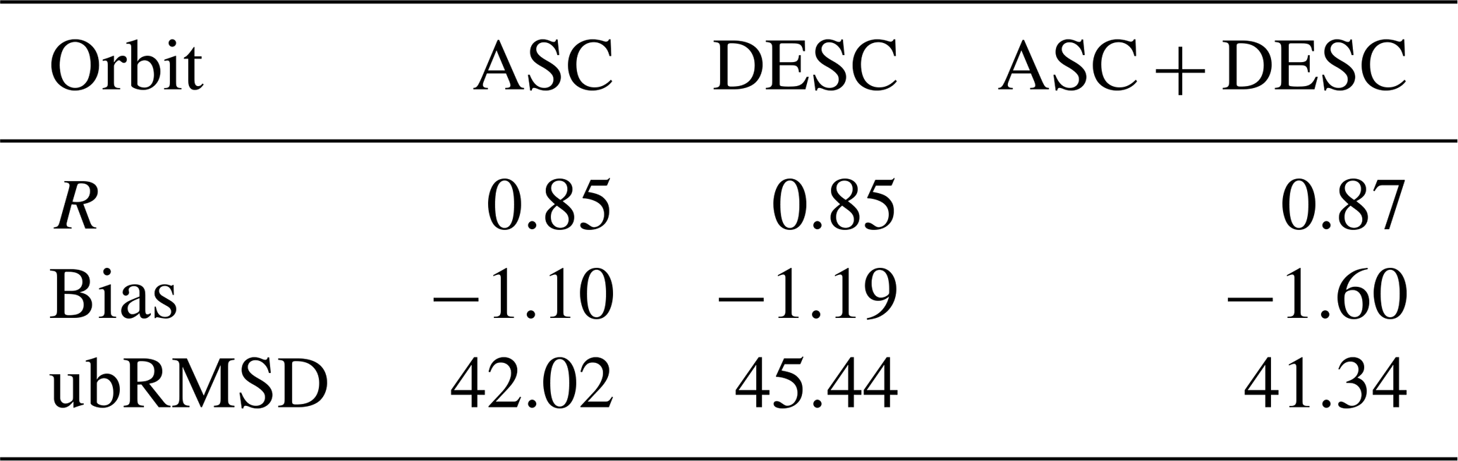
The correlation coefficients between the estimated AGB and the reference values from CCI 2018 are greater than 0.85 and are slightly higher when combining ascending and descending orbits together. Merging both orbit types also marginally decreases the ubRMSD, which is around 40–45 Mg ha⁻¹ in all configurations. The bias does not improve when combining the orbit types but remains around the same order of magnitude. This bias is below 2 Mg ha⁻¹ in absolute value. For this study, the bias is not the most important metric as it does not necessarily reflect a deviation from the true AGB value, which is unknown, as no benchmark AGB map exists. Globally, the performances are not impacted by the orbit type. Considering these results, ascending and descending orbits can properly be merged to compute the yearly L-VOD maps. It increases the number of daily VODs to compute the average and fills areas where one orbit or the other is affected by RFI.

4.1.3 Impact of a regional calibration

One important feature of this study is assessing the impact of using a single global relationship rather than several regional ones. Four regions (north, tropics, Amazon, and Africa) are considered in the analysis. They are displayed as colored rectangles in Fig. 1. The AGB estimates obtained from the calibrated global logistic function (left panel of Fig. 5) are evaluated against the AGB estimates computed from the regionally calibrated logistic functions.

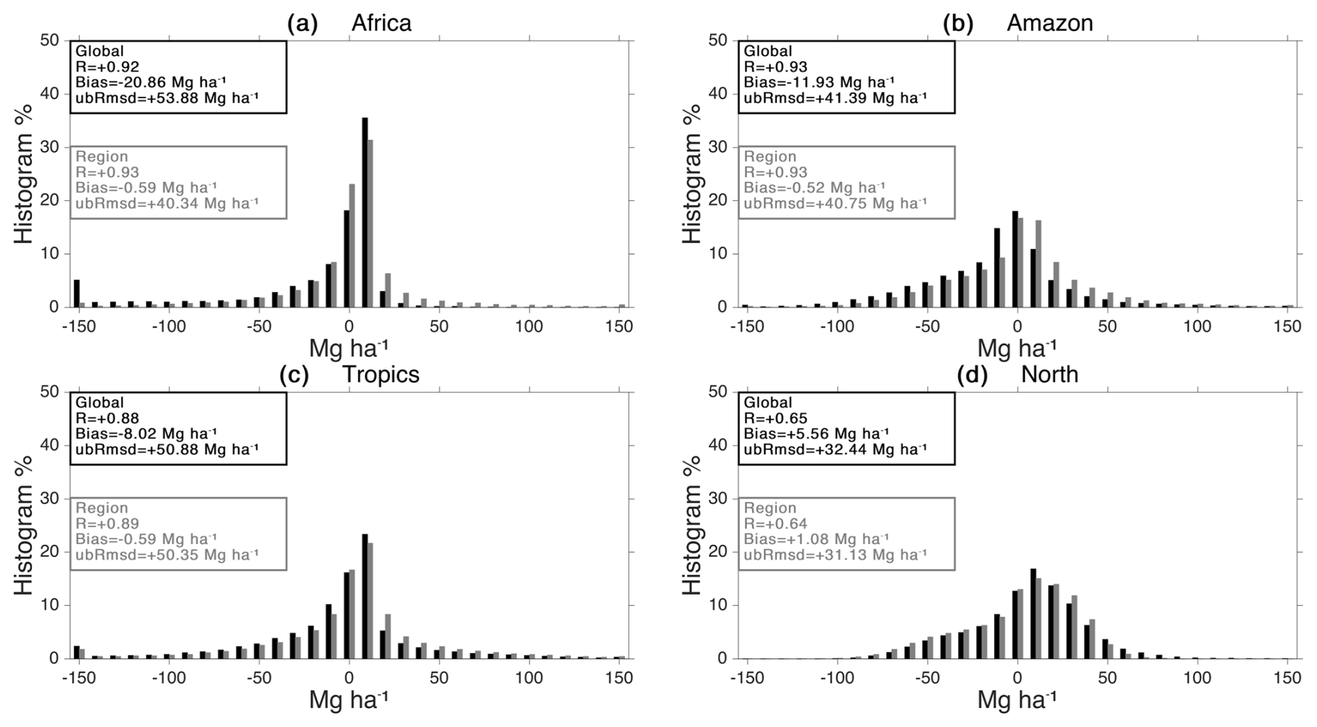
Figure 7 AGB differences between the estimation and the calibration data from CCI 2018 in the four regions identified in Fig. 1. In each panel, the black histogram represents the distribution of the differences in the study region when estimating the AGB from the global fit (global R, bias, and ubRmsd; black box), and the gray histogram represents the distribution of the differences when estimating the AGB from the regional calibration (region R, bias, and ubRmsd; gray box).

The statistics in terms of R, bias, and ubRMSD obtained with the regional and global calibrations for the four regions with respect to CCI 2018 are displayed in Fig. 7. The regional calibration does not impact R. As expected, the bias and ubRMSD are always lower with the regional fits than the global fit. The improvement is particularly important for the African continent compared to the other three regions. For Africa, the regional bias is close to zero, whereas the global bias is equal to −20.86 Mg ha⁻¹. This global bias still remains low compared to the high AGB values in the region (up to 400 Mg ha⁻¹ according to the calibration map). The regional ubRMSD is lower than the global one by 13 Mg ha⁻¹. Figure 7 also shows that the bin representing the differences higher than 150 Mg ha⁻¹ is not present with a regional calibration for Africa, which explains the bias improvement.

For the other three regions, the regional and global ubRMSD values are very close, the difference in ubRMSD being less than 1.5 Mg ha⁻¹. The regional and global difference distributions are also very similar. The bias improves by 11 and 7 Mg ha⁻¹ between the regional and the global estimations for the Amazon and the tropic regions, respectively. Again, this bias improvement is small compared to the AGB values over the tropical forests. A regional relationship is not justified for these regions.

An additional test was conducted for the particular case of the northern high latitudes (above 60° N). The boreal forests are prone to strong seasonality with extensive snow cover in winter. The impact of snow-covered acquisitions on the averaged VOD and the calibration was then evaluated. To this end, the VOD averaged over July and August was compared to the full year average. The July–August averaged VOD globally presents higher values than the full year average. The maximum of the absolute VOD differences is 0.50 and 75 % of these differences lie under 0.042. Ultimately, these differences do not significantly impact the logistic function calibration but impact the AGB estimation variability from one year to the other. In order to increase the VOD and AGB stability in the northern high latitudes, it was decided to remove to VOD acquisitions when the air temperature was below 0 °C.

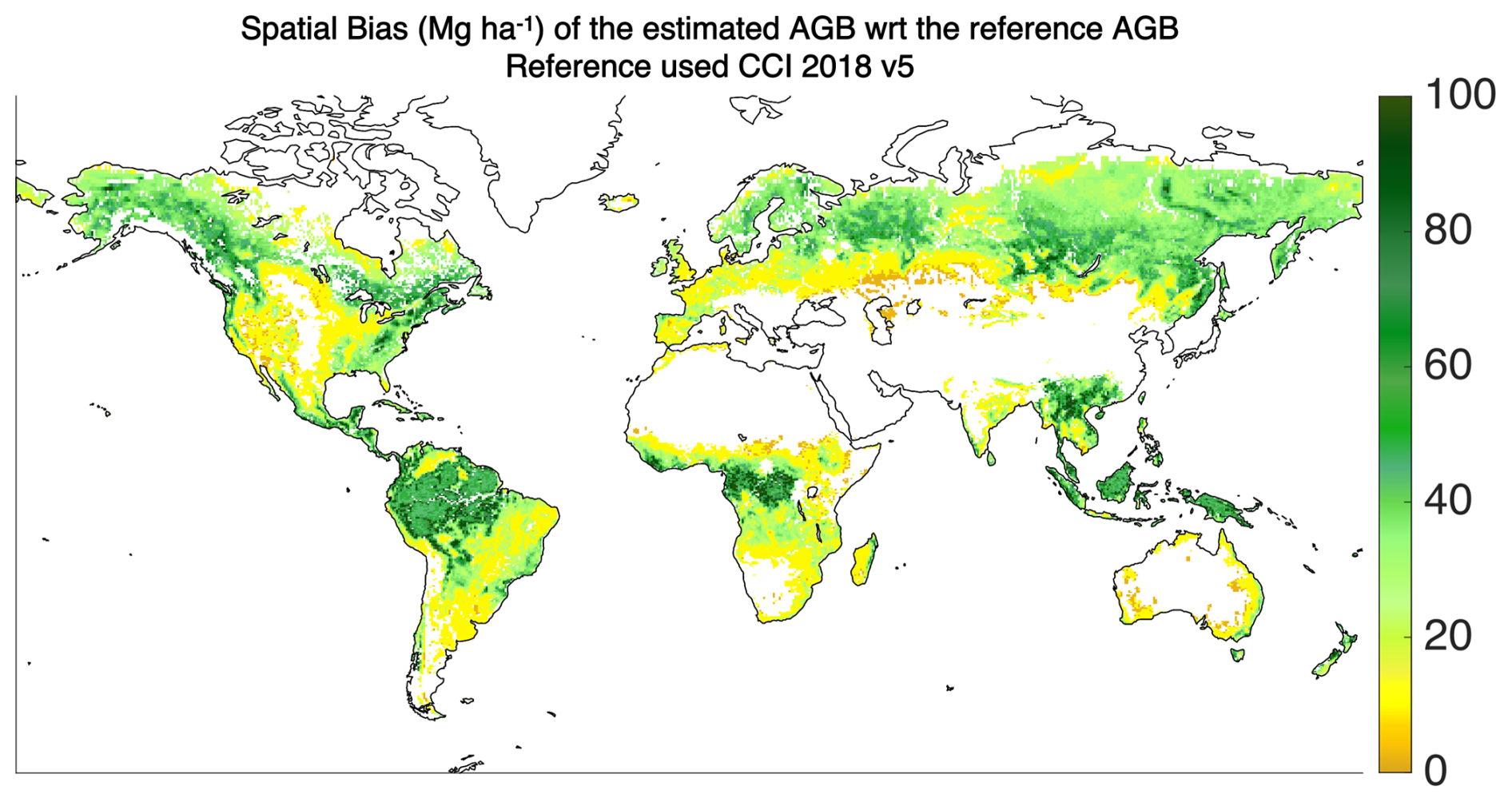
Figure 8 Spatial bias (Mg ha⁻¹) related to the logistic fit between the AGB values from the CCI 2018 and the 2018 SMOS L-VOD.

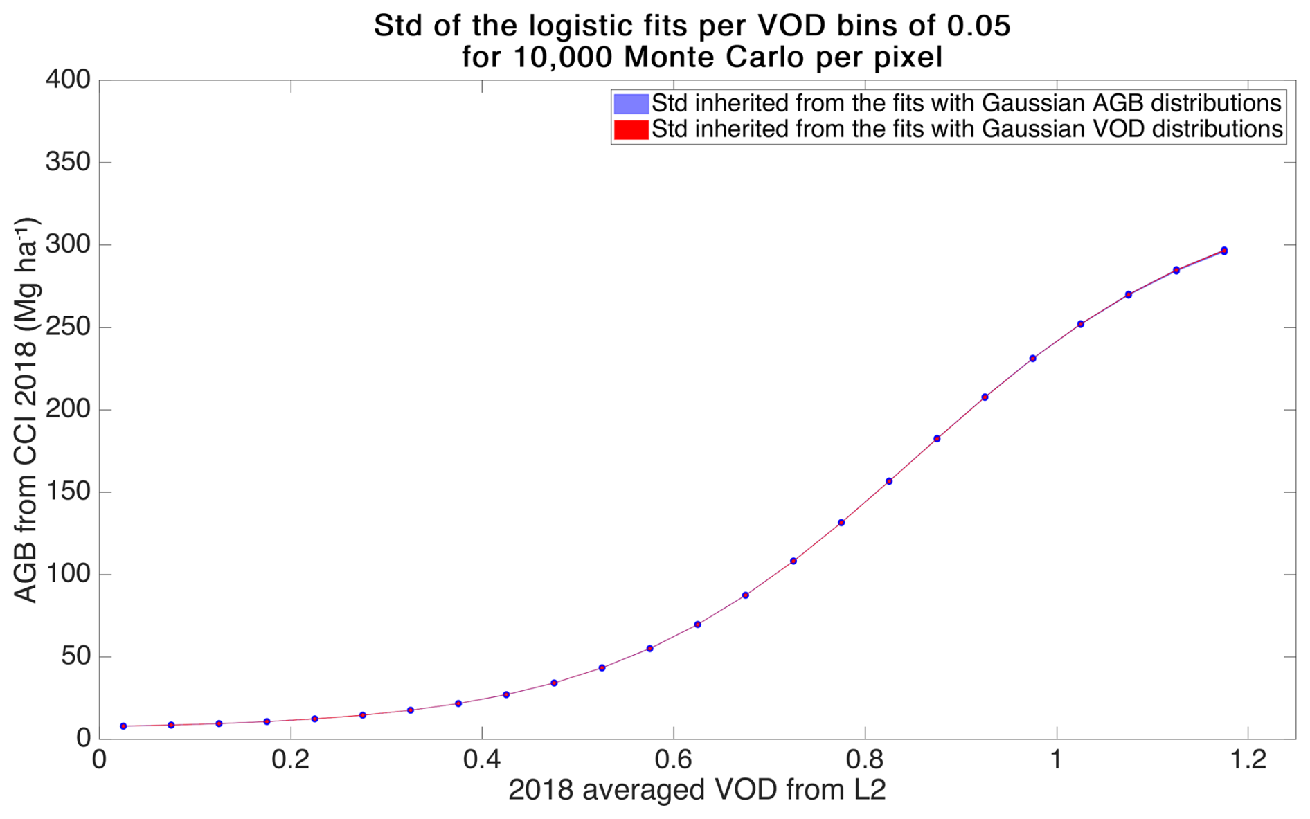
Figure 9 Standard deviation (Mg ha⁻¹) of the 10 000 Monte Carlo draws for a Gaussian AGB distribution per pixel (blue) and a Gaussian L-VOD distribution per pixel (red).

4.2 Uncertainty estimation

The two sources of uncertainty discussed in Sect. 3.2 have a different impact on the estimation. As shown by Figs. 8 and 9, the uncertainties inherited from the input data are negligible compared to the spatial bias component dominating the logistic fit uncertainties. The propagation of the reference AGB standard deviation (blue shaded area in Fig. 9) ranges from 0 to 1.5 Mg ha⁻¹. Indeed, the AGB value may vary significantly per pixel from one Gaussian draw to the other, but on average, the mean AGB–VOD distribution remains the same considering the number of points taken into account. The same result prevails for the propagation of the mean VOD_DQX (red shaded area in Fig. 9). The spatial bias is much more dynamic and ranges from 0 to 100 Mg ha⁻¹ (Fig. 8). As the standard deviation of the input AGB map is not always available and does not impact the AGB estimation, only the spatial bias component of the logistic fit (Fig. 8) is written to the output product. This component corresponds to half of the difference between the quantiles 84 and 16 and should be interpreted as a confidence interval around the mean estimated AGB value provided in the product.

4.3 Temporal analysis

4.3.1 Comparison of the estimated AGB with CCI AGB

To assess the relevance of extrapolating a spatial relationship over time, the VOD-derived AGB with a global calibration is compared with the CCI AGB available from 2015 to 2021. As shown in Table 2, the global statistics characterizing the differences between the estimated AGB and the CCI AGB values are uniform over the years. Spatially, the distribution of the differences is similar across the 7 years as shown by Fig. 10a–g. The region with the highest differences (more than 300 pixels with differences greater than 200 Mg ha⁻¹) is the equatorial part of Africa.

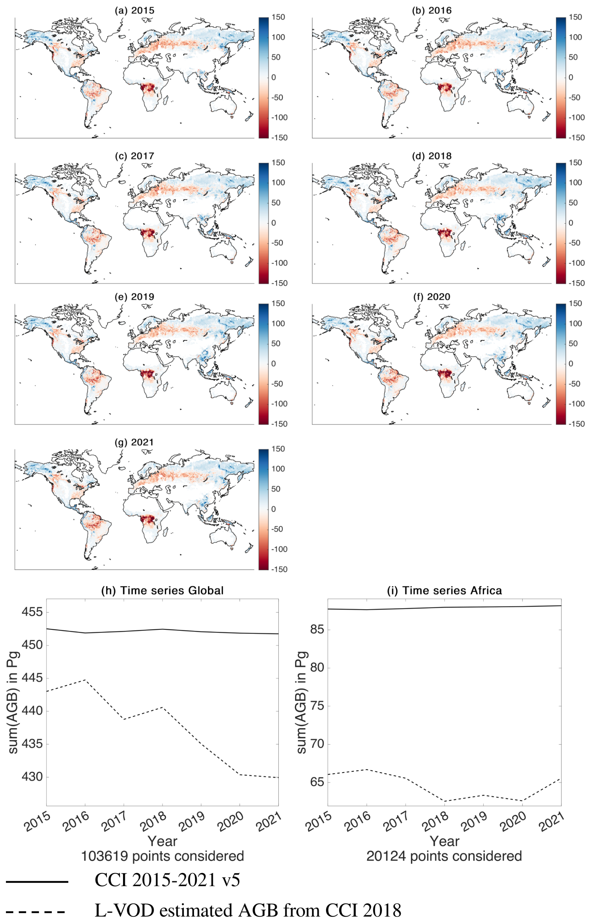
Figure 10 (a–g) Difference in Mg ha⁻¹ between the yearly AGB estimated from the 2018 global logistic fit (Fig. 5) minus CCI AGB values for the years 2015–2021. (h, i) For the global and Africa regions defined in Fig. 1, time series of the sum of the AGB from CCI (solid line) and the estimation using LVOD and CCI-2018 (dashed line).

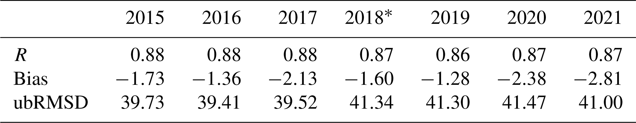
Table 2 R, bias (Mg ha⁻¹), and ubRMSD (Mg ha⁻¹) between the estimated AGB and AGB values from CCI for the years 2015–2021. AGB was estimated using the global logistic fit computed from the VOD and the CCI AGB for the year 2018. ^* Year of reference.

Additionally, the time series of the total AGB sum from both datasets over the global area and the African continent are compared against each other in Fig. 10h and i. The total AGB sum corresponds to the AGB summed over all pixels contained in a given region multiplied by the area of a pixel (always 625 km² for EASE 2 at 25 km). Only pixels common to both datasets and all 7 years are taken into account. Comparing the sum of both AGB estimates is particularly relevant, as the total AGB in a given area is often used as a proxy for the live vegetation biomass carbon stock (Liu et al., 2015; Xu et al., 2021b).

Overall, the CCI reference values are steady over time. On the global scale, the SMOS-derived AGB shows a decreasing trend, presents more variability, and has slightly lower estimations compared to the CCI. This agrees with the negative biases from Table 2. For the African continent, the AGB estimated from the VOD is on average 23 Pg lower than the reference because of the spatial differences over the equatorial part of the region.

4.3.2 Comparison of the estimated AGB with Xu AGB

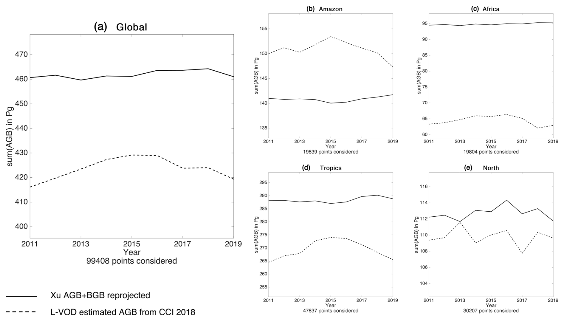
Besides the SMOS AGB estimates from this product, Xu et al. (2021b) provide the only dataset covering more than 10 years (from 2000 to 2019). A comparison of the yearly datasets over a 9-year time series (2011–2019) is performed.

The Xu et al. (2021a) estimates, converted to AGB and resampled onto the EASE 2 grid at 25 km, are summed according to the method presented in Sect. 4.3.1. The comparison of the time series between Xu et al. (2021b) and the estimated AGB using the global fit is displayed in Fig. 11 for all regions of interest. For all cases but the Amazon, the AGB estimates from the SMOS VOD are lower than Xu et al. (2021b) with higher – though not significant – interannual variability. Over the Amazonian rainforest, the AGB estimates from the SMOS VOD are on average 10 Pg higher than Xu et al. (2021b). This offset is caused by the differences between Xu et al. (2021b) and the CCI AGB. The latter, being used to calibrate the VOD, is higher than the former in most forested areas in both tropical and boreal regions (see Fig. 2e). When considering the full tropical belt, the L-VOD-derived AGB is lower than the Xu et al. (2021b) one because of the equatorial part of Africa, where the AGB estimated from SMOS does not reach the high values of Xu et al. (2021b).

Figure 11 Time series of the total sum of the AGB for the different regions defined in Fig. 1 from Xu et al. (2021b) (solid line) and the estimation using SMOS and CCI-2018 (dashed line).

5 Discussion

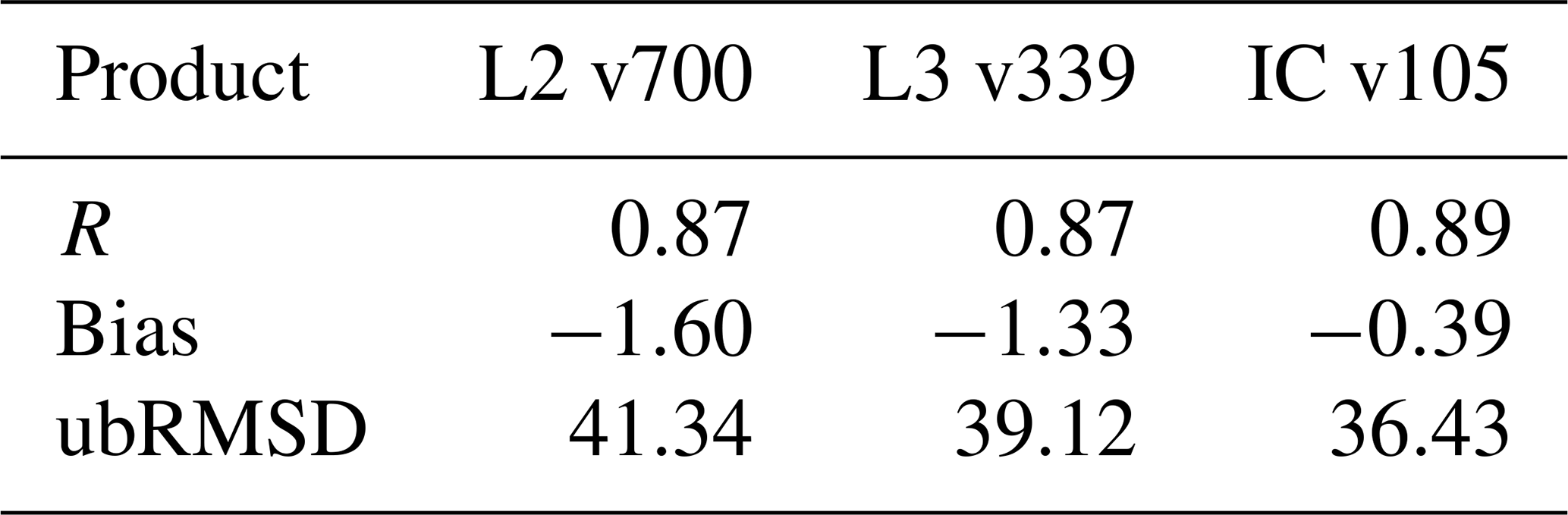
The paper describes a dataset which is a follow-up to the work initiated by Liu et al. (2015) at high frequencies (X- and C-band) and developed at L-band for SMOS by Rodríguez-Fernández et al. (2018), Fan et al. (2019), and Mialon et al. (2020). This analysis goes further and quantifies the effects of different aspects of the method on the derived AGB, which are (i) mixing the morning and afternoon overpasses, (ii) using a relationship at the global scale, (iii) extrapolating a spatial relationship over time, and most importantly (iv) providing a confidence interval range of the estimated AGB. First, the consistency of the approach is confirmed by comparing the L2 product performances with two other SMOS-derived VODs: the CATDS L3 product (Al Bitar et al., 2017) and the INRA-CESBIO (IC) dataset (Fernandez-Moran et al., 2017). This part is not detailed in the present analysis as the results are very similar. Even though the three SMOS VODs are derived with different algorithms (Kerr et al., 2012; Al Bitar et al., 2017; Fernandez-Moran et al., 2017), the approach developed in this paper leads to equivalent performances, as shown in Table 3. The IC algorithm shows higher R (0.89 versus 0.87 for L2 and L3) and slightly lower ubRMSD and bias. Nevertheless, taking into account the order of magnitude of the bias and ubRMSD differences across the three products (0.9 Mg ha⁻¹ in bias and 5 Mg ha⁻¹ in ubRMSD), they are completely negligible in comparison to the order of magnitude of the spatial bias introduced by the fitting of the logistic function (Fig. 4, 30–90 Mg ha⁻¹).

Table 3 R, bias (Mg ha⁻¹), and ubRMSD (Mg ha⁻¹) between the AGB estimated with the VOD from L2, L3, and IC mixing ascending and descending orbits and the CCI 2018 calibration data.

The effect of the time of observation is also evaluated. It is admitted that morning overpasses (06:00 LT for SMOS) offer more stable surface conditions as the Earth's surface reaches a thermal equilibrium. Therefore, better SM and VOD retrievals are expected using the morning orbits. It has, however, no impact for the present application as the three cases (i.e., only morning, only afternoon, and the two combined) have similar performances at the timescale considered in this study, with a correlation coefficient R ranging between 0.85 and 0.87 (see Table 1). The yearly averaging smooths the daily variability caused by the vegetation water content. Both overpasses (morning and afternoon) can be merged without a strong impact on the calibration. This increases the number of observations per pixel to compute the yearly VOD average and improves the coverage of regions that are either polluted with RFI or have cold temperatures during wintertime (Schwank et al., 2024).

Then, the impact of using a global relationship at the regional scale is estimated. Across the four studied regions (Fig. 1), only Africa presents a significant estimation improvement when using a regional relationship (Fig. 7). The case of the African continent is specific, as the equatorial part of the region has the highest CCI AGB values of up to 400 Mg ha⁻¹. Deriving a regional logistic relationship between the VOD and the AGB reproduces these high values better. With the global calibration, the logistic fit does not reach the 400 Mg ha⁻¹ threshold (see left panel of Fig. 5) and saturates around 300 Mg ha⁻¹. This value corresponds to the average AGB value in the Amazon rainforest according to the CCI 2018 map. Hence, applying the global relationship over Africa leads to lower estimated AGB than the CCI AGB. Moreover, the VOD values are more scattered and present more variability in central Africa compared to the VOD values in the Amazon rainforest. However, these derived AGB estimates in the equatorial part of Africa are consistent with other AGB datasets such as Avitabile et al. (2016). Adopting a single global logistic relationship between the SMOS LVOD and the input AGB is a good trade-off between performance, simplicity, and consistency.

Regarding the time dimension, the general method relies on the hypothesis that a spatial relationship for a single year is accurate enough to create the time series. Indeed, the VOD–AGB relationship is defined for a particular year and is propagated over time. This assumption, never evaluated by any studies, is tested thanks to the 7 years of the CCI dataset. The logistic relationship defined with the CCI 2018 was applied to the SMOS VOD for 2015, 2016, 2017, 2019, 2020, and 2021. The estimated AGB values are then compared to the CCI 2015–2017 and 2019–2021. The performances of the SMOS-derived AGB are similar for all years in terms of coefficient of correlation (between 0.86 and 0.88 according to Table 2) and ubRMSD (between 39.4 and 41.5 Mg ha⁻¹). The biases are also very close (around −2 Mg ha⁻¹), with better results for 2016 and 2019 (−1.36 and −1.28 Mg ha⁻¹). It supports the consistency of the VOD–AGB relationship. The main differences between the SMOS-derived AGB and the CCI AGB are observed over the tropical forests in Africa and the boreal forests of eastern Siberia. In Africa, the lower estimates are consistent for all years and are caused by the global VOD–AGB relationship (see previous comment). In this study, the CCI AGB map v5 for 2018 has been used to optimize the spatial logistic relationship. As the CCI biomass team applies a scaling factor to homogenize the yearly AGB estimates and to limit abrupt changes at the pixel scale between years (Santoro et al., 2023), the dynamic of the CCI AGB over time is low (steady black curves in Fig. 10h and i). Spatially, the CCI AGB differences from one year to the other do not exceed 2 Mg ha⁻¹ in absolute value for 99 % of the pixels. These differences fall well below the uncertainties associated with the CCI aggregated maps (up to 43 Mg ha⁻¹), which already have a low influence on the AGB estimates as demonstrated by the Monte Carlo test (Sect. 4.2). Consequently, fitting the relationship with the CCI map from another year does not significantly impact the estimation of the AGB time series.

To support the analysis, the derived time series is then compared to Xu et al. (2021b), which is the only other dataset covering more than 10 years. Differences between the two datasets are expected as they were produced from different inputs and with different methods. Xu et al. (2021b) include lidar, optical, and radar datasets, whereas SMOS is a passive microwave sensor. Radar and passive microwaves do saturate over dense vegetation but at different vegetation densities. Radar is also more sensitive to the roughness at the vegetation–air interface. For every studied region, the SMOS-derived time series show more interannual variability. This may be partly caused by the natural fluctuations of the yearly averaged L-VOD due to changes in the vegetation water content to which the L-VOD is highly sensitive. Thanks to the yearly averaging, this variability remains relatively low at ∼3 % (difference of 13 Pg over an average value of ∼424 Pg) at the global scale (left Fig. 11, dotted line). Differences also exist between the trends. For example, there is an opposite trend in the Amazon region and a peak in the northern region in 2013 not observed in Xu et al. (2021b) dataset. Such differences are expected due to the abovementioned reasons, and further investigations and intercomparisons between published and future AGB datasets will be needed to explain and understand these divergences.

Finally, this new dataset provides a confidence interval on the derived AGB, contrary to other similar databases. The derived uncertainty is mostly dominated by spatial biases, which highlights the inability of a single global model to map all the relationships between the VOD and AGB. Figure 4 presents the estimated confidence interval per bin of SMOS-derived AGB. Figure 8 is the same information projected on a map to better visualize the spatial distribution of this bias. The propagation of the uncertainties of the input data through the logistic function optimization was also carefully checked using a Monte Carlo approach. The impacts of the VOD and CCI AGB uncertainties on the AGB estimation were evaluated and found to be small (1.5 Mg ha⁻¹ for the highest AGB values) compared to the AGB spatial bias. Figure 4 also emphasizes that strong AGB values may be underestimated when computing AGB from the L-VOD and the optimized logistic function. Indeed, L-VOD tends to saturate over densely vegetated areas, even though it does not saturate as much as optical indices or VOD in C- and X-bands.

6 Data availability

The dataset is available at https://doi.org/10.12770/95f76ff0-5d89-430d-80db-95fbdd77f543 (Boitard et al., 2024). The AGB estimates from SMOS L-VOD are open-access and available at https://data.catds.fr/cecsm/Land_products/L4_Above_Ground_Biomass/ (Boitard et al., 2024). The data content description is available at https://data.catds.fr/cecsm/Land_products/L4_Above_Ground_Biomass/documentation/NT_AGB_maps_from_VOD.pdf (Boitard et al., 2023).

7 Conclusions

The paper presents the AGB dataset estimated from the SMOS L-band passive microwave VOD, which is directly related to the vegetation water content. When averaged over a year, it nevertheless constitutes a good proxy for the AGB and presents the advantage of covering a long time series, starting in 2011.

This study focuses on the method and analyzes the robustness of the approach to estimate the AGB from the SMOS Level 2 VOD. In particular, it is shown that SMOS ascending and descending orbits can and should be merged at the yearly timescale to estimate the AGB. It slightly improves the correlation with the calibration AGB (0.87 when merging orbit types versus 0.85 for ascending or descending orbits only) and decreases the ubRMSD to 41 Mg ha⁻¹. Moreover, even though a global relationship (VOD–AGB) is appropriate, slight differences are observed over Africa compared to using a dedicated relationship for this continent. Indeed, the global calibration underestimates the high AGB in the tropical region of Africa by up to 200 Mg ha⁻¹ for 300 pixels. The analysis also evaluates the multiyear dataset with two global time series. The SMOS-derived AGB dataset is very close to the CCI AGB used for its calibration (average R 0.87 over 7 years). The estimated AGB is slightly lower than the one from Xu et al. (2021b) and presents more interannual variability. The latter is directly inherited from the interannual variability of the yearly averaged SMOS L-VOD. Finally, this study provides an estimate of the uncertainties of the derived AGB for the first time in order to better assess its application in the context of biomass monitoring. This uncertainty ranges from 10 Mg ha⁻¹ for lower AGB values up to 100 Mg ha⁻¹ for AGB values around 200 Mg ha⁻¹. The present dataset is freely accessible from the CATDS website.