A regional pCO₂ climatology of the Baltic Sea from in situ pCO₂ observations and a model-based extrapolation approach

Ocean surface pCO₂ estimates are of great interest for the calculation of air–sea CO₂ fluxes, oceanic uptake of anthropogenic CO₂, and eventually the Global Carbon Budget. They are accessible from direct observations, which are discrete in space and time and thus always sparse, or from biogeochemical models, which only approximate reality. Here, a combined method for the extrapolation of pCO₂ observations is presented that uses (1) model-based patterns of variability from an empirical orthogonal function (EOF) analysis of variability with (2) observational data to constrain EOF pattern amplitudes in (3) an ensemble approach, which locally adjusts the spatial scale of the mapping to the density of the observations. Thus, data-constrained, gap- and discontinuity-free mapped fields including local error estimates are obtained without the need for or dependence on ancillary data (e.g. satellite sea surface temperature maps). This extrapolation approach is generic in that it can be applied to any oceanic or coastal region covered by a suitable model and observations. It is used here to establish a regional pCO₂ climatology of the Baltic Sea (Bittig et al., 2023: https://doi.org/10.1594/PANGAEA.961119), largely based on ICOS-DE ship of opportunity (SOOP) Finnmaid surface pCO₂ observations between Lübeck-Travemünde (Germany) and Helsinki (Finland). The climatology can serve as improved input for atmosphere–ocean CO₂ flux estimation in this coastal environment.

1 Introduction

The ocean plays a major role in the global carbon cycle and has a controlling function on the atmospheric CO₂ content on longer timescales (DeVries, 2022). Since the rise of atmospheric CO₂ concentrations since the beginning of the pre-industrial period (year 1750), the ocean has taken up ∼25 % of the CO₂ released from human activities (Friedlingstein et al., 2022), with the annual uptake mainly related to the increase in the air–sea pCO₂ imbalance. The role of coastal and continental shelf waters is more complex. Apart from atmospheric CO₂ levels, changes in nutrient loads and organic matter supply from land, changes in weathering in the drainage basin, and even changes in the functioning and composition of biological key players on various levels can lead to changes in the inorganic carbon system and thus the source–sink function of coastal seas (e.g. Laruelle et al., 2018; Müller et al., 2016; Carstensen and Duarte, 2019; Kuliński et al., 2022). Moreover, coastal seas provide an important conduit of land-derived carbon into the open ocean's interior (e.g. Thomas et al., 2004).

For the Baltic Sea, several attempts have been made to quantify the net CO₂ air–sea balance in the form of a pCO₂ climatology as well as to derive trends in surface water pCO₂, with partly contradictory results (e.g. Omstedt et al., 2009; Parard et al., 2016, 2017; Becker et al., 2021; Neumann et al., 2022; Wesslander et al., 2010). Most of the approaches either used the output from biogeochemical models or tried to create pCO₂ fields from mapped proxy data and observational data using extrapolation approaches. Seasonal mapping of pCO₂ is particularly challenging for the Baltic Sea due to its high regional and temporal variability, a salinity gradient affecting e.g. CO₂ equilibria, and a large seasonal amplitude caused by high net productivity in spring and summer and entrainment of waters enriched in remineralization products due to mixed-layer deepening in autumn and winter (Schneider and Müller, 2018).

Climatologies of pCO₂ on a global or ocean-wide scale are an important tool for the quantification of the oceanic CO₂ sink in the framework of e.g. the Global Carbon Budget (Landschützer et al., 2013; Friedlingstein et al., 2022). Tailored regional analysis can help to gain insight into changes in the source–sink behaviour of distinct regions, as recently demonstrated for the northern European shelf, including the Baltic Sea (Becker et al., 2021).

A robust climatology and trend for the Baltic Sea has, apart from refining the estimate of the net CO₂ flux in relation to the Global Carbon Budget, several implications. As the entire Baltic Sea area belongs to the territorial waters or exclusive economic zones (EEZs) of one of the pan-Baltic nations, the air–sea CO₂ fluxes might be of importance for current and future carbon management and accounting schemes in the framework of national emission reduction targets (Luisetti et al., 2020). A pCO₂ climatology could also serve as a baseline for potential negative emissions applications, including blue carbon or coastal alkalinity enhancement (GESAMP, 2019). Knowledge of monthly pCO₂ fields and their variability might also help to identify and quantify the impact of perturbations and extreme events, e.g. heat waves (Humborg et al., 2019).

In this work, we build a foundation for such applications. We first present a novel extrapolation approach, followed by construction of a Baltic Sea pCO₂ climatology. The extrapolation approach is then evaluated and put into context with existing mapping methods. Notable features of the seasonal pCO₂ climatology are discussed and special attention given to the regional long-term pCO₂ trend before we conclude our work.

2 Methods

2.1 Extrapolation approach

For mapping from scarce observational data to spatially filled maps of the Baltic Sea, we use an ensemble of truncated empirical orthogonal function (EOF) reconstructions. For a more detailed description than the brief summary below, please consult Appendix A.

EOF decomposition and singular value decomposition (SVD) have been used widely in atmospheric and ocean science (e.g. Lorenz, 1956; Weare et al., 1976; Weare and Newell, 1977; Hannachi et al., 2007). They can be used to efficiently reduce the dimensionality of the original dataset (Lorenz, 1956; Davis, 1976; Preisendorfer, 1988; Monahan et al., 2009; Jolliffe and Cadima, 2016). Here, we use the EOF decomposition of a model dataset X of pCO₂ in the Baltic Sea to obtain spatial EOF patterns e_i of pCO₂ variability.

In a second step, observational pCO₂ data Y are used in conjunction with these spatial patterns of variability in a truncated EOF reconstruction to constrain the EOF spatial patterns' amplitudes (Kaplan et al., 2000; Preisendorfer, 1988) and thus to extrapolate from scarce observational data to the full domain (Sect. A3). This step represents an optimization of a cost function Q (Eq. A19), which in our case also takes the observational data uncertainty into account to avoid overfitting (Sect. A4). For a given EOF reconstruction with l spatial modes, we thus obtain both an extrapolated field as well as an estimate of the mapping uncertainty σ_P, representing the uncertainty in the extrapolation with the given data constraints. In addition, we derive a representational error estimate ${\mathit{\sigma }}_{P^{\prime }}$ for the variance not resolved by the given EOF reconstruction due to truncation and use of just l modes (Sect. A4).

However, the choice of how many EOF modes to use for a given truncated EOF reconstruction, or at which level to truncate, is an arbitrary one often inspired by a certain threshold of the total variance explained (e.g. Kaplan et al., 2000).

In a third step, we therefore use an ensemble approach to circumvent this problem: instead of a single EOF reconstruction with a fixed number of modes l, we use a series of EOF reconstructions from just one mode up to a maximum number of l_max modes (Sect. A5). This series is then combined by a weighted ensemble at each location with the individual EOF reconstruction's mapping uncertainties as weights (Eqs. A25 and A26; Sect. A6).

Note that the weights are spatially resolved and depend on the available data constraints, i.e. the ensemble weights provide for locality, which includes adaptation of the mapping's spatial scales to the data constraint density, thus providing for a more robust extrapolation and more realistic uncertainty estimates than with a fixed number l of EOF modes.

We thus obtain an ensemble mean pCO₂ value x_reconstr, the average number of modes $\stackrel{\mathrm{‾}}{\mathit{l}}$ used in the ensemble of reconstructions at a given location, and an uncertainty estimate σ_reconstr (Eq. A28), which consists of the sample variance about the ensemble mean value, the ensemble-averaged mapping uncertainty σ_P (from each truncated EOF reconstruction with l from 1…l_max), and the ensemble-averaged representational error ${\mathit{\sigma }}_{P^{\prime }}$ (from each EOF reconstruction) (Sect. A6). All these quantities are obtained without gaps on the full spatial domain of the original model dataset X.

Finally, due to the high temporal dynamics of our Baltic Sea environment, we use an expansion of the EOF reconstruction approach to reconstruct not only the data value, but both the data value and a (short-term) linear trend, in order to temporally collate (temporally extended) observations into a time-coherent, synoptic picture (Sect. A7; Elken et al., 2019).

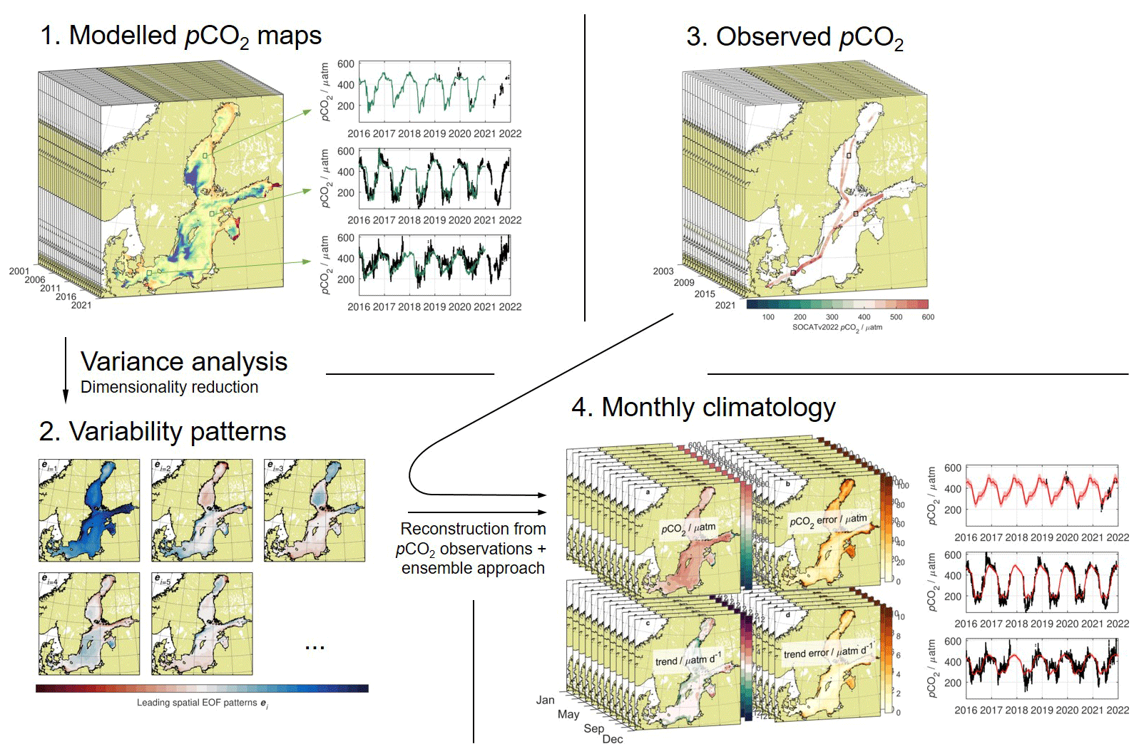
Figure 1 Approach to build a regional pCO₂ climatology of the Baltic Sea. (1) pCO₂ data from an ecosystem model are mathematically analysed for dominant patterns of variability in a truncated EOF analysis. (2) Patterns of variability and (3) pCO₂ observations of a given month are used to reconstruct Baltic Sea pCO₂ distributions $\stackrel{\mathrm{‾}}{\mathcal{X}}$, which are combined through an ensemble approach into (4) a monthly climatology of surface pCO₂, including a pCO₂ error estimate, and the (short-term) pCO₂ trend, including the pCO₂ trend error estimate. For illustration, time series are given for three sample locations for model pCO₂ (green), pCO₂ observations (black), and climatological pCO₂ (red).

2.2 Baltic Sea pCO₂ climatology

Given limitations of modelled data, we aimed to produce an observation-based pCO₂ climatology. For this, we used (a) the above extrapolation approach with spatial patterns based on ecosystem model data and (b) observations of surface pCO₂ from the Surface Ocean CO₂ Atlas (SOCAT) to produce a monthly climatology of pCO₂ as well as of the linear, short-term pCO₂ trend to temporally collate pCO₂ observations (Sect. A7) within a month (see Fig. 1 for a visualization of the approach).

2.2.1 Spatial patterns of variability

Spatial patterns of variability e_i for our extrapolation approach are based on model data from a Baltic Sea setup of the Ecological ReGional Ocean Model (ERGOM version 1.2). This version of ERGOM includes a simple carbon cycle as described in Kuznetsov and Neumann (2013) with amendments to allow for non-Redfield stoichiometry as outlined in Neumann et al. (2022). In principle, any carbon-containing biogeochemical ocean model of choice can be used as a basis for the patterns of variability e_i. Nonetheless, a better carbon representation in the model likely provides better-suited e_i patterns of variability.

The model data variability characteristics are illustrated in the Appendix (Fig. A1). Less than 1 % of the locations show a temporal decorrelation scale ≤7 d, so that we chose a weekly aggregation of the model data for variability pattern extraction. For the climatology itself, we chose a more typical monthly resolution.

ERGOM has been shown to adequately mirror observations of the large-scale nitrate, phosphate, oxygen, and carbon distribution (Neumann et al., 2022; Eilola et al., 2011; Neumann et al., 2015). However, shortcomings still exist in the exact magnitude and timing of phytoplankton carbon uptake and release throughout the seasons (Neumann et al., 2022; Fig. 4).

From an ERGOM version 1.2 model run from 1948 to 2020, we used the last 20 years of modelled surface pCO₂ from 2001 to 2020 averaged into 1044 weekly means. The model run has a horizontal resolution of 3 nautical miles, which yields a dataset X with 12 010 grid points m for the Baltic Sea area south of the Skaggerak (i.e. HELCOM subbasins 2 to 17, HELCOM Secretariat, 2017) and 1044 time steps n.

From these model data X, patterns of variability e_i were extracted by EOF analysis (see Appendix A for details). The analysis of our model data retained 224 EOF modes with a minimal cross-validation error of 22.6 µatm against the model data and a total explained variance of 98.6 %. The spatial patterns e_i have the same 3 nautical mile resolution as the model data.

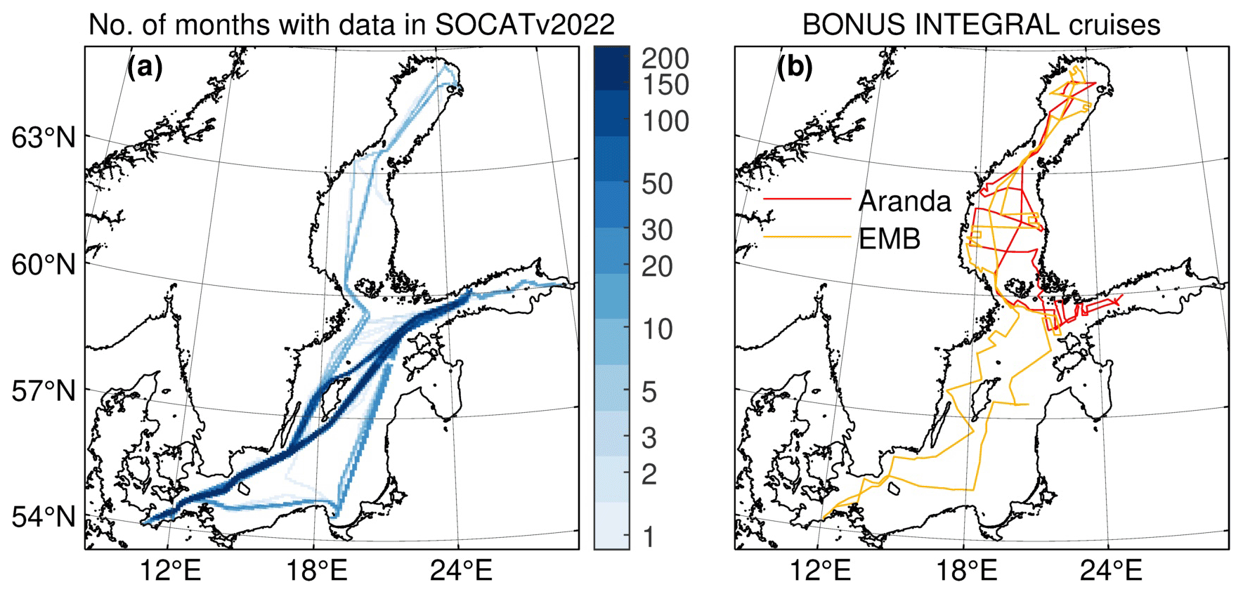
Figure 2 (a) Map of the Baltic Sea with the number of individual months with pCO₂ observations available in SOCATv2022 between June 2003 and December 2021 (maximum 223 months). (b) Cruise tracks of BONUS INTEGRAL cruises on RV Aranda in February and March 2019 and RV Elisabeth Mann Borgese in May and June 2019.

2.2.2 Surface pCO₂ observations

Surface pCO₂ measurements in the Baltic Sea were obtained from SOCAT version 2022 (Pfeil et al., 2013; Bakker et al., 2016; Bakker et al., 2022), which collects surface pCO₂ data from underway observations of ships of opportunity (SOOPs) or research vessels. All observations are based on CO₂ measurements in air equilibrated with sea surface waters (Körtzinger et al., 1996; Pierrot et al., 2009) with a typical accuracy of 2–5 µatm (in some cases ≤10 µatm), which is indicated by the respective quality flags A–E (Pierrot et al., 2009; Bakker et al., 2016).

Here, Baltic Sea pCO₂ data for the period June 2003 to December 2021 were used. They were from the ICOS-DE SOOP Finnpartner/Finnmaid line (Schneider et al., 2006; Gülzow et al., 2011) between Lübeck-Travemünde and Helsinki, which covers the southern and central Baltic Sea, or the ICOS-SE SOOP Tavastland line between Lübeck-Travemünde and Oulu or Kemi, which additionally covers the northern basins starting from 2019 (Fig. 2a). Additional surface pCO₂ data originated from RV Aranda cruise ARA04/2019 in February and March 2019 and RV Elisabeth Mann Borgese cruise EMB214 (Rehder et al., 2021) in May and June 2019 (Fig. 2b), which were carried out as part of the BONUS INTEGRAL project. Data processing and quality control followed the SOCAT guidelines. In total, data coverage in the southern and central Baltic Sea is high, with locally up to 189 out of 223 months covered (i.e. June 2003 to December 2021). Data in the northern Baltic Sea, however, are only available since February 2019, with observations during a total of 15 out of 35 months.

2.2.3 Monthly climatology construction

For every month t of the 189 months with observations, the observations were centred temporally on the 15th of each month as t_∘ (see Sect. A7), so that the extrapolation approach provides a field $\stackrel{\mathrm{‾}}{\mathcal{X}}$ with a spatial distribution of

• the reconstructed pCO₂ (x_t,reconstr, Eq. A27) at t_∘,

• the pCO₂ error estimate (σ_t,reconstr, Eq. A28) at t_∘,

• the (short-term) pCO₂ trend at t_∘,

• an error estimate of the pCO₂ trend at t_∘, and

• the average number of patterns e_i used in the reconstruction ($\stackrel{\mathrm{‾}}{\mathit{l}}$, Eq. A25)

for each month with observations (e.g. Fig. 3 for $\stackrel{\mathrm{‾}}{\mathcal{X}}$s of May 2013 as an illustration).

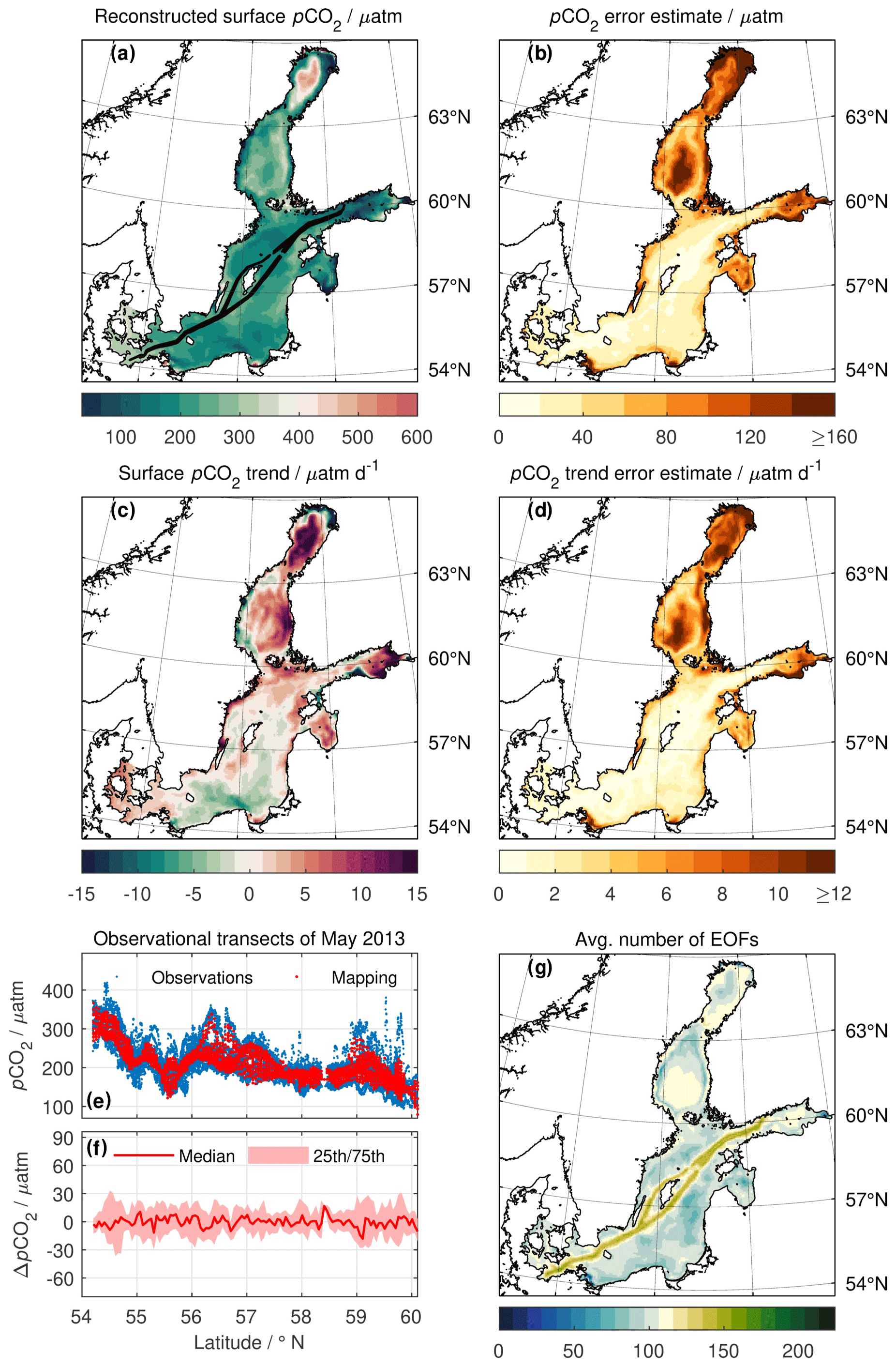
Figure 3 Monthly fields $\stackrel{\mathrm{‾}}{\mathcal{X}}$ of surface pCO₂ reconstruction for May 2013. (a) Reconstructed pCO₂ x_t,reconstr with observation locations given as black dots. (b) pCO₂ error estimate σ_t,reconstr with small values close to observations. (c) pCO₂ trend and (d) its error estimate. (e) Observed (blue) and reconstructed pCO₂ (red) against latitude as well as (f) their difference as the median (solid line) and interquartile range (pale shading). (g) Average number of patterns $\stackrel{\mathrm{‾}}{\mathit{l}}$ of the reconstruction: above-average $\stackrel{\mathrm{‾}}{\mathit{l}}$ indicates the use of high-order, smaller-scale patterns e_i, notably close to data constraints from observations, whereas below-average $\stackrel{\mathrm{‾}}{\mathit{l}}$ indicates areas where low-order, larger-scale patterns e_i dominate the reconstruction ensemble (see Eq. A26). Compare Fig. A2 for a reconstruction without a temporal trend (Sect. A7).

The construction of a monthly pCO₂ climatology for the entire Baltic Sea has its bottleneck in the temporal coverage of the northern basins, i.e. the Bothnian Sea, the Quark, and the Bothnian Bay. While the central and southern Baltic Sea has approximately 85 % of all the months covered since June 2003, observations in the northern basins only start in February 2019, with 43 % monthly coverage until the end of 2021. While the extrapolation approach provides fully filled maps of pCO₂, including the northern basins, also for months pre-February 2019, they are associated with larger uncertainties, i.e. limited explanatory power, in the northern basins (e.g. Fig. 3b). To not create a wrong impression of seasonality or interannual variability, especially if the mapping uncertainty fields σ_t,reconstr are not respected by a casual user, we chose to provide a mean seasonal climatology Y. Here, the weighting of the climatology (Eq. 1; see below) ensures the preference of reconstructions with proper observation constraints (i.e. February 2019 and onwards for the northern basins) over reconstructions without them (i.e. pre-February 2019).

For a given location m, χ_m denotes the (reconstructed) time series of $\stackrel{\mathrm{‾}}{\mathcal{X}}$ (with size 1×189) and y_m the time series of the mean monthly climatology Y (with size 1×12), respectively. The monthly means y_m were then obtained by

$$\begin{array}{}\text{(1)}& {\displaystyle }{\mathit{w}}_m\cdot {\mathit{\chi }}_m& {\displaystyle }={\mathit{w}}_t\cdot \left({\mathbf{O}}_m^{\mathbf{T}}{\mathit{y}}_m^{\mathbf{T}}+{\mathit{g}}_m\cdot (\mathit{t}-t_{\mathrm{ref}})\right)\text{with}\text{(2)}& {\displaystyle }{\mathit{w}}_m& {\displaystyle }=\mathrm{1}/{\mathit{\sigma }}_{m,\mathrm{reconstr}}^{\mathrm{2}},\end{array}$$

where w_m is the time series of inverse variance weights (Eq. 2) with size 1×189 at the given location m, O_m a time series operator or matrix of size 12×189 that selects the monthly mean y_m corresponding to the month of χ_m, t−t_ref the time difference (in decimal years) between each of the 189 monthly $\stackrel{\mathrm{‾}}{\mathcal{X}}$ and a reference time, t_ref, and g_m an extra degree of freedom to allow for a linear long-term trend in $\stackrel{\mathrm{‾}}{\mathcal{X}}$ for each location m (e.g. surface pCO₂). As a reference time, the middle of 2013 was chosen, which closely corresponds to the mean date of all the observations.

Equation (1) represents a system of 189 linear equations with 13 degrees of freedom to calculate 12 weighted mean values y_m and a long-term trend g_m. Through the inverse variance weights (Eq. 2), monthly maps χ_m with better-constrained data, i.e. smaller variance of reconstruction ${\mathit{\sigma }}_{m,\mathrm{reconstr}}^{\mathrm{2}}$ at the given location m (and for the given month), obtain preference in the weighted mean (Eq. 1).

When done for each point m, one obtains the mean seasonal climatology Y (with size m×12), centred on 2013, as well as a map of its mean linear (long-term) trend G (with size m×1) for each of the five fields $\stackrel{\mathrm{‾}}{\mathcal{X}}$ discussed.

2.2.4 Dataset description

The dataset (Bittig et al., 2023) consists of two plain-text files. One contains the mean seasonal climatology Y and the other the mean linear (long-term) trend G. Based on the 3 nautical mile resolution of the original model data, both feature 12 010 grid points m for HELCOM sub-basins 2 to 17. For the months January through to December, the climatology file gives pCO₂ (µatm), a pCO₂ error estimate (1σ) (µatm), a (short-term) pCO₂ trend for the 15th of each month (µatm d⁻¹), a (short-term) pCO₂ trend error estimate (1σ) (µatm d⁻¹), and the average number of patterns ($\stackrel{\mathrm{‾}}{\mathit{l}}$) (see Figs. A3 and A4). The long-term trend file gives both the long-term linear trend G (µatm yr⁻¹) (Fig. 7) and its error estimate (1σ) (µatm yr⁻¹).

3 Results

3.1 Extrapolation approach

The mapping approach gives fully filled fields on the entire spatial domain from scattered observational data. The mapped pCO₂ is in a similar range and frequency distribution to observations with improvements in terms of distribution and correlation over the original model pCO₂ (Fig. 4a). The mapped fields are smooth and without spatial gaps or discontinuities. The pCO₂ error estimate is reduced in the spatial vicinity of observations. In contrast, pCO₂ error is markedly increased both near shore as well as in sub-basins not covered by observations, e.g. the northern basins or the Gulf of Riga for a SOOP Finnmaid-based reconstruction (e.g. Fig. 3b). Still, pCO₂ values remain within reasonable margins even in those areas (e.g. Fig. 3a). We cannot observe a tendency of the mapping approach to give extreme values or outliers in the absence of observations (compare Fig. 4a). Rather, with few or no data constraints, variability pattern e_i amplitudes in the ensemble tend towards zero, i.e. towards zero deviation, which is equivalent to the spatially resolved temporal mean pCO₂ of the model (Appendix A).

Addition of a linear temporal trend to collate observations to a common time t_∘ helps to reduce the mismatch between temporally spread observations and a full-domain mapping of a dynamic coastal system (compare e.g. Figs. 3e, f and A2c, d, respectively).

However, for about half the grid points of the 189 monthly mappings, the magnitude of the short-term temporal pCO₂ trend (e.g. Fig. 3c) at a given location m is insignificant, i.e. within its trend error estimate (e.g. Fig. 3d). At the same time, a considerable portion of the significant pCO₂ trends is found at grid points m in the direct footprint of observations where the trend error estimates are small in the first place. This demonstrates that a monthly temporal resolution is sufficient for construction of a Baltic Sea pCO₂ climatology with our approach.

3.2 Quality of interpolation and extrapolation

To assess the quality of the obtained fields, we consider (a) the mapped result against the original observations and (b) a comparison of mappings from concurrent subsets of observations.

For the first aspect, we consider the residual pCO₂ against SOCAT observations for all 189 monthly mapped fields from the climatology construction (e.g. Fig. 3e, f). We use typical metrics for interpolation methods (correlation, bias, standard deviation). As the monthly fields $\stackrel{\mathrm{‾}}{\mathcal{X}}$ were constructed from those observations, this assesses primarily to which degree the data constraints were taken into account for the mapping, e.g. the balance between point-to-point reproduction and smoothing with the given patterns of variability e_i.

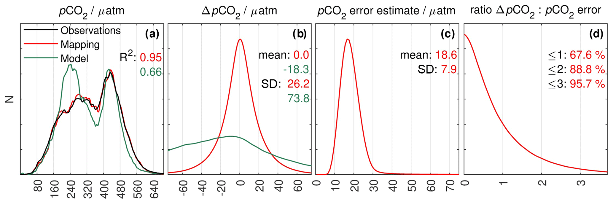
Figure 4 Histograms for (a) pCO₂ observations (black) as described in Sect. 2.2.2, pCO₂ reconstructed at the observation times and locations from the 189 monthly mappings (red), and model pCO₂ extracted at the observation times and locations (green). Reconstructed and observed pCO₂ data are highly correlated (R²), and they show a similar distribution. Correlation between modelled and observed pCO₂ is weaker, and their distributions show noticeable differences. (b) The pCO₂ difference between reconstructed (red) or modelled (green) pCO₂ and observed pCO₂. There is no bias in the reconstruction, while differences between model and observations show a much wider range than the reconstructed pCO₂. (c) The pCO₂ error estimates σ_reconstr of the reconstruction at the observation times and locations. (d) The ratio between the pCO₂ difference and pCO₂ error estimate, where a ratio ≤1 means that the observed pCO₂ is within 1×σ_reconstr of the mapped pCO₂.

The comparison shows highly correlated pCO₂ data (R²=0.95), a similar pCO₂ distribution (Fig. 4a), and an unbiased mapping with a standard deviation of 26 µatm (Fig. 4b). This includes both misfits of the mapped fields as well as variations within observations of a given grid point location (compare the spread between observations and mapping in Fig. 3e). The error estimate is of a similar magnitude (Fig. 4c) and is well collocated. That is, residuals are within 1× the error estimate in 68 % of the cases (Fig. 4d).

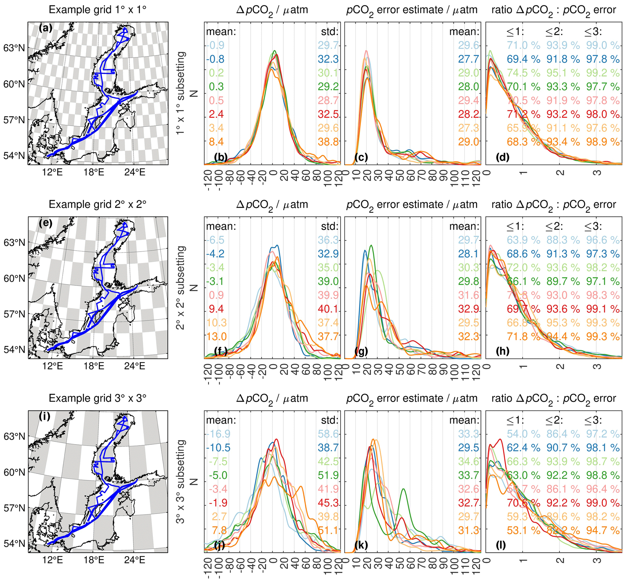
Figure 5 Subsetting evaluations for May 2019 observations using 1^∘ × 1^∘ subsets (top row; a–d), 2^∘ × 2^∘ subsets (middle row; e–h), and 3^∘ × 3^∘ subsets (bottom row; i–l), respectively, with maps (a, e, i) illustrating one example subsetting grid where observations (blue) in white boxes are used for pCO₂ reconstruction and observations in grey boxes for evaluation. Histograms are for (b, f, j) the pCO₂ difference between reconstructed and observed pCO₂ within the evaluation boxes. (c, g, k) The pCO₂ error estimate σ_reconstr of the reconstruction at the observation times and locations within the evaluation boxes. (d, h, l) The ratio between the pCO₂ difference and pCO₂ error estimate within the evaluation boxes, where a ratio ≤1 means that the observed pCO₂ is within 1×σ_reconstr of the mapped pCO₂. The colours represent eight different 1^∘ × 1^∘, 2^∘ × 2^∘, and 3^∘ × 3^∘ subsetting grids only offset spatially in latitude and longitude.

The second aspect, how data constraints in one area transfer to accurate predictions in another part of the domain, is more difficult to assess objectively. It requires the observational data to be split into a subset that is used for mapping and a subset that is deemed independent and used for evaluation. How this subsetting is done, however, directly influences the outcome of the evaluation. That is, while such evaluations may seem instructive and generalizable, they are highly dependent on design and thus carry some degree of arbitrariness.

To illustrate this, we consider a series of monthly mappings for May 2019, the month with the highest density of observations in our 189 monthly mappings. We use chessboard-like grids with alternating white and black boxes for subsetting, where observations in the white boxes are used for mapping and observations in the black boxes are used for evaluation. Grid box sizes vary from 1^∘ × 1^∘, 2^∘ × 2^∘, to 3^∘ × 3^∘ subsetting grids (see Fig. 5a, e, and i for example grids). To check for dependence on a specific data distribution, the 1^∘ × 1^∘, 2^∘ × 2^∘, and 3^∘ × 3^∘ subsetting grids were shifted spatially in latitude and longitude so that every grid size had eight different realizations, each with different sets of data in the mapping and evaluation subsets, respectively (Fig. 5).

For 1^∘ × 1^∘ subsetting, the eight realizations show a relatively coherent picture: differences ΔpCO₂ between mapped and observed pCO₂ (Fig. 5b) are slightly larger (by 5–12 µatm) than for interpolated data (Fig. 4b) and are mostly unbiased. pCO₂ error estimates are elevated (Fig. 5c vs. Fig. 4c), while the ratio of differences and error estimates, i.e. the collocation of bias and error estimate, shows a similar distribution for both extrapolation (Fig. 5d) and interpolation (Fig. 4d). With increasing spatial scales of the 2^∘ × 2^∘ and 3^∘ × 3^∘ subsetting, pCO₂ differences and error estimates become larger, as would be expected (Fig. 5f, j and g, k). Encouragingly, however, the ratio of differences and error estimates preserves a similar shape (Fig. 5h, l). That is, the mapping approach seems to provide suitable mapping error estimates.

More concerning, however, are increasing differences between the eight realizations with increasing spatial scales. Especially for the 3^∘ × 3^∘ subsetting, some realizations show a pCO₂ bias, which additionally can be different between realizations (blue vs. orange realizations, Fig. 5j), as well as noticeable differences in pCO₂ error estimates and thus mapped pCO₂ (e.g. green realization, Fig. 5k). This illustrates a strong dependence on the specific choice of subsetting, i.e. which data are included in mapping and which data are excluded for validation.

We conclude that, with a given choice of subsetting, one implicitly chooses which statistical values one wants to get out. While our evaluation could be described as being well designed, it turns out to be starting-point-dependent. If a month with less data coverage were chosen, differences between realizations (i.e. which data end up in the training or validation subset) would be even larger. Therefore, based on the above illustration, any subsetting-based evaluation needs to be taken with a sufficient amount of caution, as the subsetting design will imprint itself on the outcome.

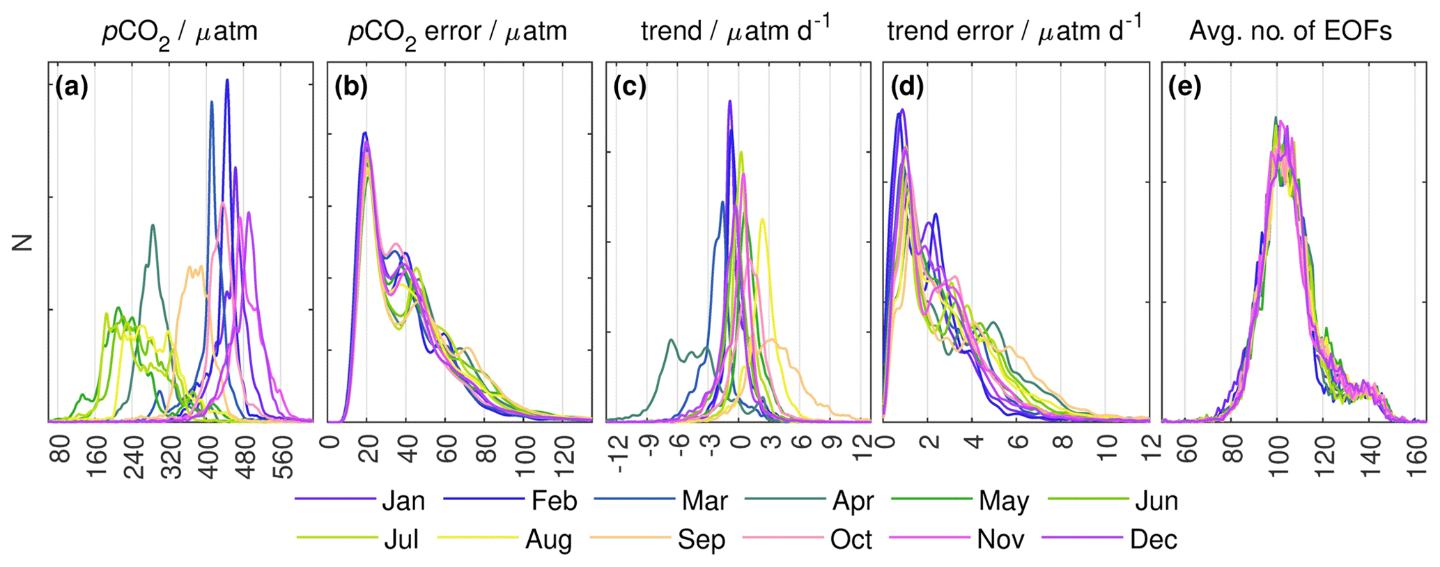
Figure 6 Smoothed histograms for the five output fields of the climatology Y: (a) reconstructed pCO₂ x_t,reconstr, (b) pCO₂ error estimate σ_t,reconstr, (c) pCO₂ short-term trend, (d) error estimate in the pCO₂ short-term trend, and (e) the average number of patterns $\stackrel{\mathrm{‾}}{\mathit{l}}$ used in the reconstruction. The colour code indicates the respective month. pCO₂ follows a typical seasonal cycle, while the pCO₂ error estimate and the number of patterns show no apparent seasonal variations. pCO₂ trends show higher magnitudes during spring (March and April) and late summer (August and September), which is mirrored by enhanced pCO₂ trend error estimates in these months.

3.3 Baltic Sea pCO₂ climatology

3.3.1 pCO₂ distribution

The mean seasonal pCO₂ distribution x_reconstr matches previously published seasonal cycles of surface pCO₂ in the western and central Baltic Sea (Schneider and Müller, 2018): a strong spring bloom pCO₂ drawdown occurs between March and May to a low around 200 µatm in May, some slight increase in June, and a second summer bloom low in July, followed by relaxation towards atmospheric levels in September and October and supersaturated levels during late autumn and winter, peaking around 500 µatm in December (Fig. 6a; Figs. A3 and A4, first column).

Regionally, the western basins lead the mean seasonal cycle, while the central Gotland Basin and the Gulf of Finland trail behind. The productive season is even shorter in the northern basins, with the major pCO₂ drawdown in the Bothnian Sea occurring in June (Figs. A3 and A4, first column). Similarly, the seasonal amplitude is less pronounced in the western or northern basins than in the Gotland Basin and is most intense in the Gulf of Finland. For the northern basins, this is the first fully seasonal climatology from pCO₂ observations.

The pCO₂ error estimate σ_reconstr shows a minimum of 12 µatm. Close to observations, the pCO₂ error estimate of the mean seasonal climatology is of the order of 20 µatm and as such close to the value of the individual mappings (compare Fig. 6b and Fig. 4c). Further away, σ_reconstr increases up to a level around 90 µatm (95th percentile), with a spatial preference for high σ_reconstr in the northern basins as well as in the Gulf of Riga, the Oder Bight, and other sheltered, near-shore areas (Figs. A3 and A4, second column).

3.3.2 pCO₂ short-term trends

In general, the short-term pCO₂ trends follow the mean seasonal pCO₂ cycle with on average negative trends, i.e. decreasing pCO₂, during winter and spring. Positive trends prevail during late summer and autumn (Fig. 6c), with the strongest trend magnitudes occurring in the northern Baltic proper and the Gulf of Finland (Figs. A3 and A4, third column).

However, in 8 out of the 12 months, the majority of estimated trends are insignificant. That is, more than 70 % are smaller than their error estimate, indicating that inclusion of a short-term trend in the mapping may not be required for these months. Only in March and April as well as in August and September are the majority of pCO₂ trends significant (despite elevated pCO₂ trend error estimates occurring at the same time in some areas; see Fig. 6d). That is, significant short-term pCO₂ trend magnitudes fall together with the strong springtime pCO₂ drawdown as well as with autumnal mixed-layer deepening and entrainment of high-pCO₂ waters (Fig. 6; more in Jacobs et al., 2021).

Like for the pCO₂ distribution, trend error estimates are higher in the northern basins as well as the Gulf of Riga, Oder Bight, and other sheltered, near-shore areas (Figs. A3 and A4, fourth column).

3.3.3 Number of patterns or mapping scales

The average number of patterns $\stackrel{\mathrm{‾}}{\mathit{l}}$ per month can be seen as a qualitative indicator to show preference for reconstructions with larger or smaller spatial scales, respectively, in the weighted mean (Eq. A25) of the reconstruction.

For the climatology Y, $\stackrel{\mathrm{‾}}{\mathit{l}}$ shows a maximum around 105 patterns (Fig. 6e). This level is at about 45 % of the maximum number of patterns, i.e. indicating only a slight preference for reconstructions with larger-than-average scales in the weighted mean. However, a notable fraction with a higher number of patterns $\stackrel{\mathrm{‾}}{\mathit{l}}$ and a peak around 140 patterns exists (Fig. 6e). These are located in the vicinity of the observations, where the preference in the weighted mean is for reconstructions with stronger small-scale features (see e.g. Fig. 3g).

There is no seasonal imprint on the average number of patterns $\stackrel{\mathrm{‾}}{\mathit{l}}$, which is in contrast to the pCO₂ and pCO₂ short-term trend distributions (Fig. 6).

3.4 Long-term pCO₂ trend

The mean climatology Y is constructed from the 189 monthly mappings $\stackrel{\mathrm{‾}}{\mathcal{X}}$ and a linear long-term trend G (see Eq. 1 and Sect. 2.2.3). For pCO₂, the analysis shows a significant long-term pCO₂ increase of $+\mathrm{1.4}\pm \mathrm{0.5}$ µatm yr⁻¹ (1σ) in the southern Baltic Sea from the Great Belt to the Bornholm Basin and southern parts of the Gotland Basin (Fig. 7). A similar increase ($+\mathrm{1.5}\pm \mathrm{0.7}$ µatm yr⁻¹) is obtained in selected regions of the northern Baltic proper, the Åland Sea, and the Gulf of Finland. A positive trend in pCO₂ is also visible in coastal areas along the Finnish coast in the northern basins as well as in the Gulf of Riga. However, multi-year observations in those areas are unavailable to support a long-term pCO₂ trend (see Sect. 2.2.2; Fig. 2). In all the other areas, the data available do not indicate a significant long-term trend, i.e. one that is outside the 68.3 % (1σ) confidence bound. This includes in particular the western and eastern Gotland Basin but also the northern basins (Fig. 7), where the observational time series is likely too short to allow for the detection of a significant long-term trend (Fig. 2).

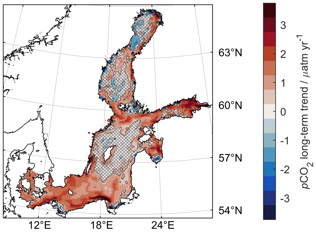
Figure 7 Long-term trend G of surface pCO₂ from the monthly mappings and the climatology construction (Eq. 1). Areas where the long-term trend is not significant are cross-hatched. In the southern Baltic Sea, a significant increase of +1.4 µatm yr⁻¹ is obtained from the observations. Selected parts of the northern Baltic proper, the Åland Sea, and the Gulf of Finland give a similar increase of +1.5 µatm yr⁻¹, while the western and eastern Gotland Basin show no significant long-term trend.

4 Discussion

4.1 Extrapolation approach

The extrapolation approach uses an EOF analysis of the data covariance Q as a foundation. When working with an EOF reconstruction, one needs to bear in mind the purely mathematical nature of the EOF modes' e_i construction. They are built by (1) maximizing the (partial) variance they explain and by (2) being orthogonal to all previous EOF modes (Preisendorfer, 1988; Monahan et al., 2009; Dommenget, 2015). They may therefore indicate some causal connection within the original data X, which requires confirmation by other means. They may, however, just as well group some portion of (partial) variance in one part of the domain with some portion of (partial) variance in another part of the domain just to mathematically maximize the amount of (partial) variance of the given EOF mode e_i. This can give rise to apparent EOF-mode “teleconnections”, where one part of the data or spatial domain is seemingly tightly coupled to another part of the data, e.g. for the second EOF mode e_i=2, which always has a dipole pattern. Often, there is a temptation to attribute such couplings or “teleconnections” to a driving mechanism. However, given its origin, patterns of EOF modes should be interpreted with great caution (and only with ancillary, supporting data) and are best seen to be of a mathematical rather than mechanistic nature (Monahan et al., 2009; Dommenget, 2015). We therefore did not try to assign physical mechanisms or drivers to specific EOF patterns e_i in our work.

The use of EOF modes as a basis for extrapolation ensures that the extrapolated map covers the full spatial domain, that it is gap-free, and that it is discontinuity-free.

A key aspect of truncated EOF reconstructions is the number l of significant modes included. Our cross-validation approach provided a relatively large number of l_max=224 modes. The relatively large number of modes is a prerequisite for a small representational error P^′, i.e. for the covariance not resolved by the collection of truncated EOF modes, which gives a lower bound on the uncertainty of the mapping σ_reconstr (Eq. A28). In our case, the average ${\mathit{\sigma }}_{P^{\prime }}$ when using all 224 patterns e_i amounts to 14.7 µatm. If only the first 50 patterns e_i were included, the average representational error would be as high as 29.1 µatm.

A reconstruction with a small number of modes provides for a more uniform, large-scale homogeneous field, where gaps in the data are filled by the large-scale picture. However, such reconstructions may lack the flexibility to reproduce real features of the observations, e.g. through too strong smoothing. Conversely, a large number of modes provides for a fine, small-scale field with high flexibility. However, features in some areas without nearby observations may be badly constrained with the risk of “ghost” signals.

By using an ensemble of reconstructions that cover the entire range of 1…l_max modes and by using the mapping variance ${\mathit{\sigma }}_P^{\mathrm{2}}$ as weights (Eqs. A25 and A26), we find an optimal trade-off in our mapping approach, where both aspects are balanced. In this way, the scales used in the mapping are adjusted spatially according to the distribution of observations as constraints.

The cost function of the mapping approach minimizes the residual between observations and mapped data (Eq. A19). In this way, a synoptic pCO₂ mapping is obtained. If observations, however, are temporally extended compared to the system's temporal dynamics, the pCO₂ mapping can be distorted and cannot represent a synoptic picture, depending on the spatial and temporal pattern by which observations are obtained (Elken et al., 2019).

The introduction of a temporal trend at each location (Sect. A7) as an additional degree of freedom reduces such distortion caused by sampling. It both improves the fit to the data (compare Fig. A2c, d vs. Fig. 3e, f) and provides extra information.

• For a given mapping, a strong or weak trend indicates where temporal dynamics are high or low and informs on where the frequency of observations should be enhanced or not, respectively.

• For a time series of mappings, information on both the value and trend allows for a more accurate interpolation by a cubic Hermite spline (Appendix B) compared to a standard, linear interpolation of the values alone (e.g. Fig. 8).

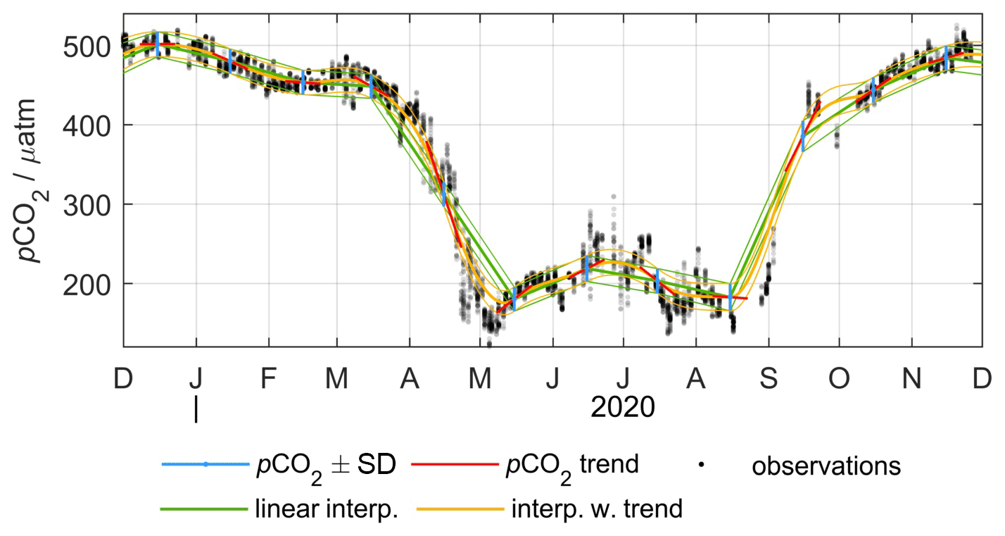
Figure 8 Difference between monthly point-by-point interpolation (green) or interpolation with a trend (orange) in a dynamic coastal system. Example data are from the northern Baltic proper (approximately 58^∘45^′ N, 021^∘00^′ E), with pCO₂ observations X shown in black. They are the basis for monthly mapped fields $\stackrel{\mathrm{‾}}{\mathcal{X}}$ of surface pCO₂ (blue) as well as for a linear (short-term) pCO₂ trend (red). Compared to a linear interpolation between monthly pCO₂ values (green), interpolation including the trend information (orange) gives a better reproduction of the observed dynamics, particularly in spring and autumn. A cubic Hermite spline was used for the calculation (Appendix B).

For our mapping of surface pCO₂ in monthly intervals, we conclude that the inclusion of a temporal trend in the mapping is required, particularly for spring and autumn. For months without strong trends, we do not see adverse effects in the mapped pCO₂ compared to an extrapolation without inclusion of a temporal trend.

The dynamics of the pCO₂ field are prescribed by the model data covariance matrix Q (Fig. A1a). The closer the model and real-world variability match, the easier it is for the mapping to reflect reality and to provide a most realistic picture. Nonetheless, also for a model dataset X that may lack some real-world features or their magnitude, the observational constraints provide an improvement in the mapped field compared to the original model (Fig. 4).

The mapping error estimates are elevated where observations are scarce or dynamics are high to start with. For our pCO₂ mapping, the model covariance Q is the origin of a pronounced coast–basin difference in the pCO₂ variance caused by both physical and biological drivers in the model. This prescribed data covariance distribution is retained in the mapping error estimates σ_reconstr. For example, they are enlarged in dynamic river plumes, in the sheltered, shallow Gulf of Riga, or in other near-shore areas, unless there are observations to constrain dynamics and thus reduce σ_reconstr. In regions with few observations, σ_reconstr approaches the prescribed data variance from Q (Fig. A1a).

We do not observe a seasonality in the number of patterns $\stackrel{\mathrm{‾}}{\mathit{l}}$ of the mapping (Fig. 6e). At the same time, the pCO₂ value varies strongly between seasons. In addition, there is a slight preference for observations to occur in spring, summer, and autumn over winter months. However, there is no discernible difference in the spatial coverage of pCO₂ observations between seasons (data not shown). The aseasonality of $\stackrel{\mathrm{‾}}{\mathit{l}}$ can be explained by the “large-scale” mapping error σ_P, used for the ensemble weights (Eq. A26) to only depend on the distribution of samples H_t and their respective observational error estimates S. Therefore, the extrapolation approach does not discriminate or distinguish by (pCO₂) value, and there is no seasonal imprint in the number of patterns.

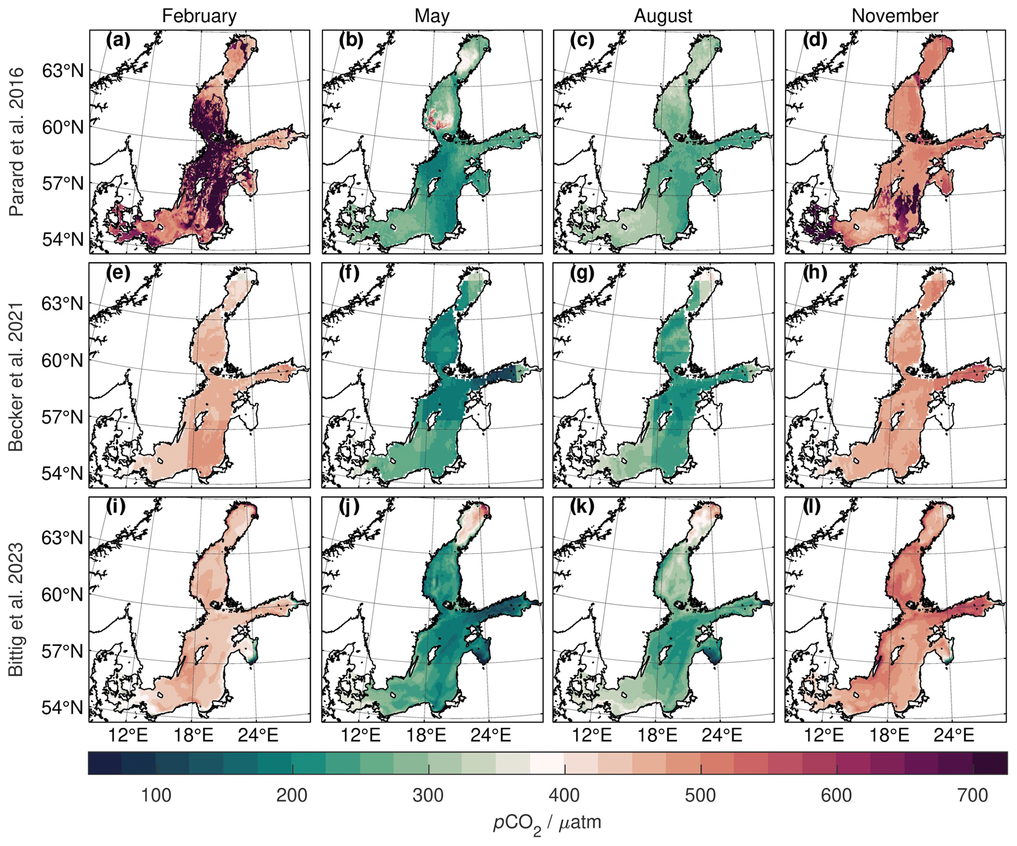
Figure 9 Mean monthly pCO₂ distribution for 1 month per season (left to right) for different climatologies: Parard et al. (2016) (a–d), Becker et al. (2021) (e–h), and this work (i–l). The first two climatologies are proxy-based, where artefacts of the proxy directly translate to pCO₂, e.g. for wintertime satellite retrievals (a, d) or the subtle 5^∘ × 4^∘ gridding in Becker et al. (2021) (e–h). Our approach uses observed pCO₂ data directly for mapping, which gives fewer artefacts but is only applicable when pCO₂ observations are available.

4.2 Comparison with other pCO₂ mapping approaches

SOCAT observations have been used previously to build surface pCO₂ climatologies of the Baltic Sea (see Fig. 9 for examples). They rely on observation-driven extrapolation approaches, which can be grouped into different categories: (a) one where sparse data points are extrapolated based on some statistic metric of influence, e.g. a spatial decorrelation length or timescale, and (b) one where parametrizations with proxy data in combination with filled fields of those proxies are used for extrapolation (Rödenbeck et al., 2015).

Our mapping approach belongs to the first category. For a given month or time window, we use the available pCO₂ data directly and one to one without an added transformation to inform the extrapolated pCO₂ map. As a (spatial) metric of influence, the variability patterns are used. This gives a direct link between observations of a given month or time window and the mapped field. Conversely, if there are no pCO₂ observations in a given time window, this directly translates to a (time) gap in the mapped fields for any approach of the first category.

Most previous pCO₂ mappings in the Baltic Sea belong to the second category (e.g. Parard et al., 2016; Becker et al., 2021). In a first step, they use all available pCO₂ data together with collocated proxies (e.g. location, sea surface temperature, chlorophyll-a concentration, water depth, distance to the coast, season) to establish a relationship or parametrization between proxies and pCO₂. In a second step, distributions of those proxy parameters are used to establish a pCO₂ distribution in time and space. Here, pCO₂ data of a given month do not directly inform the extrapolated pCO₂ map but only indirectly through the established relationship using all the data. Conversely, if there are no pCO₂ observations in a given time window but proxy data are available, they can be used to estimate a pCO₂ map nonetheless. That is, (temporal) gap filling is possible with the two-step procedure of approaches of the second category.

As a drawback, mapped pCO₂ fields of the second category rely on the validity of the proxy relationship and, equally important, on good proxy input data. In some cases, e.g. satellite-based sea surface temperature or chlorophyll-a concentration, proxies may be (seasonally) prone to artefacts, e.g. due to stronger cloud cover in winter months. Such artefacts then directly translate into mapped pCO₂ fields and may create unrealistic patterns or out-of-range values (e.g. Fig. 9a, d; Parard et al., 2016). A mapping approach of the first category such as the one presented here, which uses the observations directly, is not affected by external-source data quality (Fig. 9i–l).

Wesslander et al. (2010)Wesslander et al. (2010)Laruelle et al. (2018)Schneider and Müller (2018)Becker et al. (2021)Becker et al. (2021)

Table 1 Summary of long-term pCO₂ trends for different areas and time periods in the Baltic Sea as obtained from different studies.

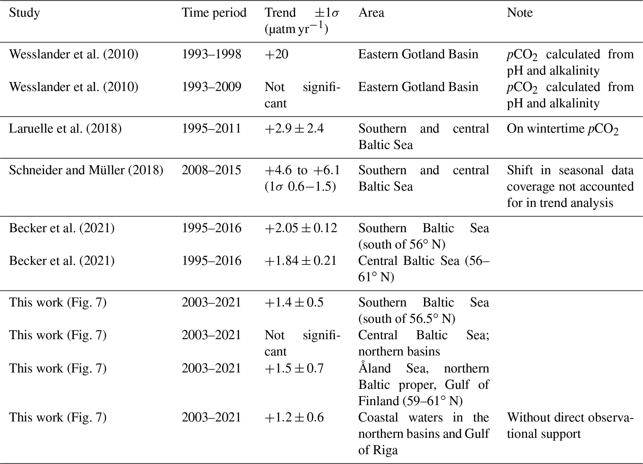
4.3 Long-term pCO₂ trend

The long-term trend of surface pCO₂ in Baltic Sea surface waters has been studied before (Table 1): Wesslander et al. (2010) describe an increase in monthly pCO₂ (approximately +20 µatm yr⁻¹) for the 1993–1998 period in the eastern Gotland Basin, which seems mostly driven by less intense summer pCO₂ minima (from approximately 50 µatm in 1993 to approximately 250 µatm in 1998). For the longer period 1993–2009, they do not detect a significant trend. While Wesslander et al. (2010) use pCO₂ calculated from pH and alkalinity, all further studies are based on the same surface pCO₂ observations archived in SOCAT (Bakker et al., 2016), albeit using different methods and time extents.

Laruelle et al. (2018) found an increase of $+\mathrm{2.9}\pm \mathrm{2.4}$ µatm yr⁻¹ (1σ) for wintertime pCO₂ from 1995 to 2011 in the southern and central Baltic Sea. At the same time, they see a similar spatial gradient to our work (Fig. 7) with a stronger increase in the south-west and a zero or even negative trend in the northern Gotland Basin.

Schneider and Müller (2018) describe an increase of +4.6 to +6.1 µatm yr⁻¹ (1σ between 0.6 and 1.5 µatm yr⁻¹) for different areas for the 2008–2015 period. However, their analysis did not deseasonalize the observations prior to linear trend analysis. During their analysed period, there is an increase in observations during autumn and winter (with typically high pCO₂) and a decrease in early spring observations (with typically low pCO₂), while late-spring and summer observations have a similar data coverage over the years. Their relatively high pCO₂ trend estimate therefore seems to be partially caused by a seasonal shift in data availability that was left unaccounted for in the analysis.

Becker et al. (2021) derived trends of $+\mathrm{2.05}\pm \mathrm{0.12}$ µatm yr⁻¹ for the southern Baltic Sea (south of 56^∘ N) and $+\mathrm{1.84}\pm \mathrm{0.21}$ µatm yr⁻¹ for the central Baltic Sea (between 56 and 61^∘ N) for the period 1995–2016. However, they observe a stronger trend in earlier years (starting in the 1990s) than for later periods (starting in the mid-2000s).

Our analysis covers the more recent period 2003–2021 and gives significant trends of $+\mathrm{1.4}\pm \mathrm{0.5}$ µatm yr⁻¹ (1σ) in the southern Baltic Sea (south of 56.5^∘ N) and $+\mathrm{1.5}\pm \mathrm{0.7}$ µatm yr⁻¹ in the Åland Sea, parts of the northern Baltic proper, as well as the Gulf of Finland (between 59 and 61^∘ N). The central Baltic Sea and the northern basins themselves show no significant trend. The positive trend ($+\mathrm{1.2}\pm \mathrm{0.6}$ µatm yr⁻¹) in coastal waters of the northern basins along the Finnish coast as well as in the Gulf of Riga (Fig. 7) currently has no support from direct observational constraints in those areas (Fig. 2). In contrast, it likely originates from high similarity to other coastal waters (e.g. along the southern Baltic shore) in the model data variability analysis and thus in the variability patterns e_i used for mapping. As such, the pCO₂ increase may be realistic but lacks field data support.

Together with the literature, our results seem to indicate a reduction in overall surface pCO₂ increase in the Baltic Sea during the past decades or even its complete absence like in the central Baltic Sea (Fig. 7) in recent periods. While atmospheric pCO₂ levels are still rising (approximately +2.4 µatm yr⁻¹ in the past decade; Lan et al., 2022), this has implications for the CO₂ balance between the atmosphere and the Baltic Sea. This supports previous claims of coastal seas becoming a less intense source of CO₂ or eventually turning into (an increasing) CO₂ sink (Laruelle et al., 2018).

5 Data availability

Surface pCO₂ data are available from SOCAT (https://doi.org/10.25921/1h9f-nb73, Bakker et al., 2022; Bakker et al., 2016) and Rehder et al. (2021). ERGOM model output data are available at https://thredds-iow.io-warnemuende.de/thredds/catalogs/projects/integral/catalog_pocNP_V04R25_3nm_agg_time.html?dataset=IOW-THREDDS-Baltic_pocNP_V04R25_3nm_agg_time_2020-11-20-12 (Neumann, 2021). The climatology is available from Bittig et al. (2023): https://doi.org/10.1594/PANGAEA.961119.

6 Conclusions

In this work, we developed an extrapolation approach that combines two worlds: models, specifically the distribution and connectivity that exist in model data variability; and observations in that they provide constraints of the real-world picture.

The most notable features of the approach are that it does not tend to give extreme, out-of-range values even with few data constraints and that it provides local error estimates, which reflect both underlying variability, e.g. coast–basin gradients, and observational data constraints. We consider of particular merit the fact that the extrapolation scheme adapts its spatial scales to the number of observations in a certain area, leading to a sound representation of less uncertainty where more data are available.

Used together with high-quality surface pCO₂ data from SOCAT, we established a climatology that covers the entire Baltic Sea. Given the present data scarcity in the northern basins of the Baltic Sea, a mean pCO₂ climatology is what is reliably achievable today. It can serve as a seasonal baseline of regional pCO₂ evolution that enables assessment of interannual variations, e.g. with respect to timing or amplitude. With sustained and/or enhanced observations in such data-poor regions, a fully monthly resolved pCO₂ dataset will become realistic in the future. To this end, SOOP Tavastland and SOOP Silja Serenade (crossing between Stockholm and Helsinki) provide a positive outlook for uncertainty reduction. Both SOOP lines were recently adopted by ICOS.

Finally, our extrapolation approach as well as the method to establish a climatology are not limited to pCO₂ or the Baltic Sea. Instead, they are transferable to other areas and parameters where the present work can serve as a template.

Appendix A: Extrapolation approach

A1 Notation and mathematical background

To represent a spatial dataset at a given time t with m spatial points, we use the data vector x_t with size m×1. For a spatial time series of n times, we use the data matrix X with size m×n, where the n columns correspond to n data vectors x_t. Data in x_t and X are the deviation from the space-dependent temporal mean ${\stackrel{\mathrm{‾}}{\mathit{x}}}_m$. The empirical data covariance matrix Q_XX with size m×m is given by

$$\begin{array}{}\text{(A1)}& {\mathbf{Q}}_{\mathbf{XX}}={\displaystyle \frac{\mathrm{1}}{n-\mathrm{1}}}{\mathbf{XX}}^{\mathrm{T}}.\end{array}$$

The singular value decomposition (SVD) or empirical orthogonal function (EOF) decomposition of the data matrix X decomposes X into a series of orthonormal factors or principal components according to

$$\begin{array}{}\text{(A2)}& \mathbf{X}=\mathbf{E}\mathbf{\Sigma }{\mathbf{A}}^{\mathrm{T}},\end{array}$$

where E is a m×m orthonormal matrix, Σ a m×n rectangular diagonal matrix, and A a n×n orthonormal matrix. With the above convention on m and n, the column vectors e_i (with size m×1) in E represent spatial patterns, while the column vectors a_i (with size n×1) in A represent amplitude time series. They are also called left-singular vectors and right-singular vectors, respectively. The diagonal elements of Σ are the so-called singular values s_i of X. Equation (A2) can be written in vector form as

$$\begin{array}{}\text{(A3)}& {\displaystyle }{\mathit{x}}_t=\mathbf{E}\mathbf{\Sigma }{\mathit{a}}_t=\mathbf{E}{\mathit{\alpha }}_t,\end{array}$$

where α_t=Σa_t is the so-called dimensional amplitude at a given time t.

Based on a SVD of X (Eq. A2), the m×m matrix B=XX^T can be expressed as

$$\begin{array}{}\text{(A4)}& \mathbf{B}={\mathbf{XX}}^{\mathrm{T}}=\mathbf{E}\mathbf{\Sigma }{\mathbf{A}}^{\mathrm{T}}\mathbf{A}{\mathbf{\Sigma }}^{\mathrm{T}}{\mathbf{E}}^{\mathrm{T}}=\mathbf{E}\mathbf{\Sigma }{\mathbf{\Sigma }}^{\mathrm{T}}{\mathbf{E}}^{\mathrm{T}}=\mathbf{E}\stackrel{\mathrm{̃}}{\mathbf{\Lambda }}{\mathbf{E}}^{\mathrm{T}},\end{array}$$

where $\stackrel{\mathrm{̃}}{\mathbf{\Lambda }}$ is a diagonal matrix whose diagonal elements are ${\stackrel{\mathrm{̃}}{\mathit{\lambda }}}_i=s_i^{\mathrm{2}}$. Equation (A4) states the eigendecomposition of B. Since matrix B is proportional to the covariance matrix Q (Eq. A1), we can state the eigendecomposition of the data covariance matrix Q as

$$\begin{array}{}\text{(A5)}& \mathbf{Q}=\mathbf{E}\mathbf{\Lambda }{\mathbf{E}}^{\mathrm{T}},\end{array}$$

with corresponding eigenvalue problem

$$\begin{array}{}\text{(A6)}& \mathbf{QE}=\mathbf{\Lambda }\mathbf{E}\end{array}$$

and

$$\begin{array}{}\text{(A7)}& \mathbf{\Lambda }={\displaystyle \frac{\mathrm{1}}{n-\mathrm{1}}}\stackrel{\mathrm{̃}}{\mathbf{\Lambda }}.\end{array}$$

The spatial patterns e_i with size m×1 are eigenvectors of the data covariance matrix, and the diagonal elements λ_i of Λ the corresponding eigenvalues λ_i, which give the amount of variance associated with each e_i. From the set of eigenvectors e_i and their corresponding amount of variance λ_i, the spatial distribution x_t at a given time t can be reconstructed by determination of a suitable amplitude vector a_t (Eq. A3) (see textbooks of linear algebra or statistical data analysis, e.g. Dommenget, 2015).

A2 Truncation of eigenvalue modes

For practical purposes, reconstruction often uses only the first l leading eigenvectors instead of all m eigenvectors e_i ($\mathrm{1}\le l\le m$). That is, E, Λ, and A are split into a matrix E, Λ, and A of size m×l, l×l, and n×l, respectively, which contain the first l leading eigenvector modes, and a matrix E^′, Λ^′, and A^′, which contain the remaining m−l eigenvector modes. Equations (A2), (A3), and (A5) thus become

$$\begin{array}{}\text{(A8)}& {\displaystyle }\mathbf{X}=\mathbf{E}\mathbf{\Sigma }{\mathbf{A}}^{\mathrm{T}}+{\mathbf{E}}^{\prime }{\mathbf{\Sigma }}^{\mathbf{\prime }}{{\mathbf{A}}^{\prime }}^{\mathrm{T}},\text{(A9)}& {\displaystyle }{\mathit{x}}_t=\mathbf{E}\mathbf{\Sigma }{\mathit{a}}_t+{\mathbf{E}}^{\prime }{\mathbf{\Sigma }}^{\prime }{a}_t^{\prime },\text{ and}\text{(A10)}& {\displaystyle }\mathbf{Q}=\mathbf{E}\mathbf{\Lambda }{\mathbf{E}}^{\mathrm{T}}+{\mathbf{E}}^{\prime }{\mathbf{\Lambda }}^{\mathbf{\prime }}{{\mathbf{E}}^{\prime }}^{\mathrm{T}}=\mathbf{P}+{\mathbf{P}}^{\prime }.\end{array}$$

The leading eigenvector modes e_i cover most of the data variance and often represent more “large-scale” spatial patterns, while the modes higher than l contain only a small amount of the data variance and can be seen as “small-scale” spatial patterns (Lorenz, 1956; Kaplan et al., 2000; Dommenget, 2015). Correspondingly, the first and second terms in Eq. (A10) give the large-scale and small-scale variances P and P^′, respectively, whereas in Eq. (A8) and its vector form Eq. (A9) they give the large-scale and small-scale contributions, respectively, to the spatial data vector x_t.

This split can also be interpreted as decomposition into a “signal” part and a “noise” part. Equations (A8)–(A10) with only the l leading modes (i.e. with only the first term) are called a truncated EOF reconstruction in which dimensionality is reduced from m to l modes. Higher-order modes (in E^′ and Λ^′, i.e. the second term) are assumed to be dominated by noise and error and are discarded in a truncated eigenvector or EOF reconstruction (Lorenz, 1956; Kaplan et al., 2000).

A3 Extrapolation from observational data

To represent a set of k observations at a given time t, we use the observational data vector y_t and the observational error σ_t, both with size k×1. The transfer operator H_t is then a “sampling” or observation function that depends on the spatial configuration of the observation points and samples from the data vector x_t of size m×1 so that the result ${\widehat{\mathit{x}}}_t$,

$$\begin{array}{}\text{(A11)}& {\widehat{\mathit{x}}}_t={\mathbf{H}}_t{\mathit{x}}_t,\end{array}$$

has the same size k×1 as the observations. To be comparable with ${\widehat{\mathit{x}}}_t$, the observational data y_t are expressed as a deviation from the space-dependent temporal mean ${\stackrel{\mathrm{‾}}{\mathit{x}}}_m$ too (Elken et al., 2019).

The eigenvalue reconstruction in truncated form (Eq. A9) then becomes

$$\begin{array}{}\text{(A12)}& {\mathbf{H}}_t{\mathit{x}}_t={\mathbf{H}}_t\mathbf{E}\mathbf{\Sigma }{\mathit{a}}_t.\end{array}$$

Minimization of a suitable cost function Q, e.g. for least-squares optimization as in Elken et al. (2019),

$$\begin{array}{}\text{(A13)}& {\displaystyle }Q\left({\mathit{\alpha }}_t\right)& {\displaystyle }={\left({\mathbf{H}}_t\mathbf{E}{\mathit{\alpha }}_t-{\mathit{y}}_t\right)}^{\mathrm{T}}\left({\mathbf{H}}_t\mathbf{E}{\mathit{\alpha }}_t-{\mathit{y}}_t\right),\text{with }\text{(A14)}& {\displaystyle }{\mathit{\alpha }}_t& {\displaystyle }=\mathbf{\Sigma }{\mathit{a}}_t,\end{array}$$

yields a system of l linear equations with l unknowns (Elken et al., 2019):

$$\begin{array}{}\text{(A15)}& {\displaystyle }\mathbf{D}{\mathit{\alpha }}_t& {\displaystyle }=\mathit{h},\text{with }\text{(A16)}& {\displaystyle }\mathbf{D}& {\displaystyle }={\mathbf{E}}^{\mathrm{T}}{\mathbf{H}}_t^{\mathrm{T}}{\mathbf{H}}_t\mathbf{E}\text{ and}\text{(A17)}& {\displaystyle }\mathit{h}& {\displaystyle }={\mathbf{E}}^{\mathrm{T}}{\mathbf{H}}_t^{\mathrm{T}}{\mathit{y}}_t,\end{array}$$

which provides the observation-based eigenvector amplitudes α_t or a_t (Eq. A14), respectively.

With Eq. (A9) in truncated form and Eq. (A14), the data vector x_t can be obtained, i.e. an extrapolation from k×1 observational data points y_t to the entire spatial domain of m×1 data points x_t with the help of the truncated eigenvalue decomposition of m×l eigenvectors and l eigenvalues e_i and λ_i, or E and Λ, respectively.

A4 Error considerations

Both “observational error” and “representational error” impact the determination of the eigenvector amplitudes a_t. Observational error σ_t includes both instrumental and sampling error and can be used to limit the impact of observational data constraints y_k (Kaplan et al., 2000). Representational error is the error made by truncation, i.e. by using only the l largest, leading eigenvectors and neglecting the remainder of the spectrum, which can be derived from the “small-scale” covariance P^′ contribution (Kaplan et al., 2000).

The error covariance matrix ℛ is the sum of the observational data error covariance S and a term that accounts for the covariance created in the truncated modes E^′ not resolved by the analysis:

$$\begin{array}{}\text{(A18)}& \mathcal{R}=\mathbf{S}+{\mathbf{H}}_t{\mathbf{E}}^{\prime }{\mathbf{\Lambda }}^{\prime }{{\mathbf{E}}^{\prime }}^T{{\mathbf{H}}_t^{\prime }}^T=\mathbf{S}+{\mathbf{H}}_t{\mathbf{P}}^{\prime }{{\mathbf{H}}_t^{\prime }}^T,\end{array}$$

where S is a diagonal matrix with the observations' variance ${\mathit{\sigma }}_t^{\mathrm{2}}$ on the diagonal and H_t is the aforementioned sampling operator (Kaplan et al., 2000).

By addition of constraints on the cost function Q (a) to limit the estimated eigenvector amplitudes based on the amount of variance they explain in the original eigenvalue decomposition and (b) that a_t determination is limited by the uncertainty of observations and from truncation (see above), Eq. (A13) is modified to (Kaplan et al., 2000)

$$\begin{array}{}\text{(A19)}& Q\left({\mathit{\alpha }}_t\right)={\left({\mathbf{H}}_t\mathbf{E}{\mathit{\alpha }}_t-{\mathit{y}}_t\right)}^{\mathrm{T}}{\mathcal{R}}^{-\mathrm{1}}\left({\mathbf{H}}_t\mathbf{E}{\mathit{\alpha }}_t-{\mathit{y}}_t\right)+{\mathit{\alpha }}_t^{\mathrm{T}}{\mathbf{\Lambda }}^{-\mathrm{1}}{\mathit{\alpha }}_t,\end{array}$$

and the solution Eqs. (A15)–(A17) thus become (Kaplan et al., 2000)

$$\begin{array}{}\text{(A20)}& {\displaystyle }\mathbf{D}{\mathit{\alpha }}_t& {\displaystyle }=\mathit{h},\text{with }\text{(A21)}& {\displaystyle }\mathbf{D}& {\displaystyle }={\mathbf{E}}^T{\mathbf{H}}_t^{\mathrm{T}}{\mathcal{R}}^{-\mathrm{1}}{\mathbf{H}}_t\mathbf{E}+{\mathbf{\Lambda }}^{-\mathrm{1}}\text{ and}\text{(A22)}& {\displaystyle }\mathit{h}& {\displaystyle }={\mathbf{E}}^{\mathrm{T}}{\mathbf{H}}_t^{\mathrm{T}}{\mathcal{R}}^{-\mathrm{1}}{\mathit{y}}_t.\end{array}$$

On the other hand, the large-scale portion of the data covariance Q (Eq. A10) can be obtained from this solution according to Kaplan et al. (2000):

$$\begin{array}{}\text{(A23)}& \mathbf{P}={\mathbf{ED}}^{-\mathrm{1}}{\mathbf{E}}^{\mathrm{T}}.\end{array}$$

P can be seen as the mapping uncertainty of the extrapolation.

Note that the calculation of P only requires the sampling operator H_t, i.e. where samples are present, as well as an observational error estimate S, but not the actual observations or amplitudes at these locations. In the absence of any observation, H_t contains only zeros and Eqs. (A21) and (A23) then simplify to $\mathbf{D}={\mathbf{\Lambda }}^{-\mathrm{1}}$ and P=EΛE^T (compare Eq. A10), respectively. Addition of observational constraints thus reduces the mapping uncertainty P.

For our purposes, we assume that off-diagonal elements in the covariance P^′ are negligible, i.e. that the truncated eigenvector modes E^′ are sufficiently small-scale and that their variances Λ^′ are small enough that they do not show a noticeable covariance contribution (Eq. A18). We therefore approximate P^′ by a diagonal matrix whose diagonal elements are obtained from rearrangement of Eq. (A10):

$$\begin{array}{}\text{(A24)}& {\displaystyle }\mathrm{diag}\left({\mathbf{P}}^{\prime }\right)=\mathrm{diag}\left(\mathbf{Q}\right)-\mathrm{diag}\left(\mathbf{E}\mathbf{\Lambda }{\mathbf{E}}^{\mathrm{T}}\right),\end{array}$$

where Q is accessible from the data X (Eq. A1) and the second term from the truncated eigenvalue decomposition.

A5 Number of significant modes

A critical aspect before any extrapolation from observations is how many modes e_i to use, or – in other words – where to truncate reconstruction, i.e. how to distinguish between modes representing desired variability and modes representing “noise”. Often, an arbitrary threshold of the total variance covered by the l leading modes is chosen (e.g. Kaplan et al., 2000).

Here, we apply the DINEOF (Data Interpolating Empirical Orthogonal Functions) variant of SVD or EOF decomposition of the dataset X to find the l_max leading eigenvectors e_i. The number l_max of significant modes is determined by a cross-validation procedure from the data X (Beckers and Rixen, 2003), and we use this l_max as the upper bound for l in our ensemble approach (see below).

A6 Ensemble approach for robustness and locality

Depending on the spatial distribution or clustering of observations y_t, not all amplitudes of the l_max spatial eigenvectors e_i may be well constrained. In some configurations, e.g. with few or clustered observations, where H_t selects only a few of the m spatial data points, a reconstruction with fewer modes than l_max may give a solution with a smaller mapping uncertainty P than the truncated reconstruction with all l_max modes e_i.

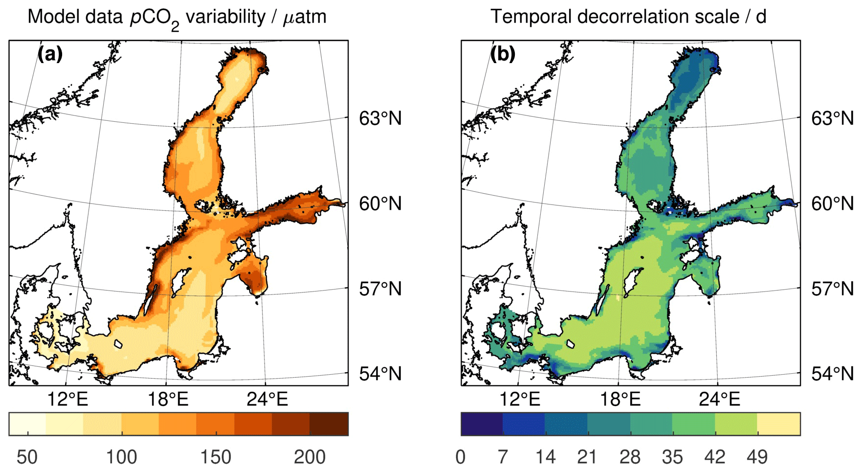
Figure A1 Model data X characteristics: (a) pCO₂ variability shown by the square root of the model data covariance matrix Q's diagonal elements, i.e. the standard deviation of the pCO₂ data X at each location. (b) pCO₂ variability shown by the temporal decorrelation timescale, i.e. the time (d) at which the lagged autocorrelation drops below a threshold of 0.63 correlation. Less than 1 % of the locations have a temporal decorrelation scale of ≤7 d, while about 25 % are within ≤30 d. To adequately reflect the pCO₂ data dynamics in the variability pattern extraction (Sect. 2.2.1), a weekly aggregation of the model data X was therefore chosen compared to e.g. daily or monthly model output.

.

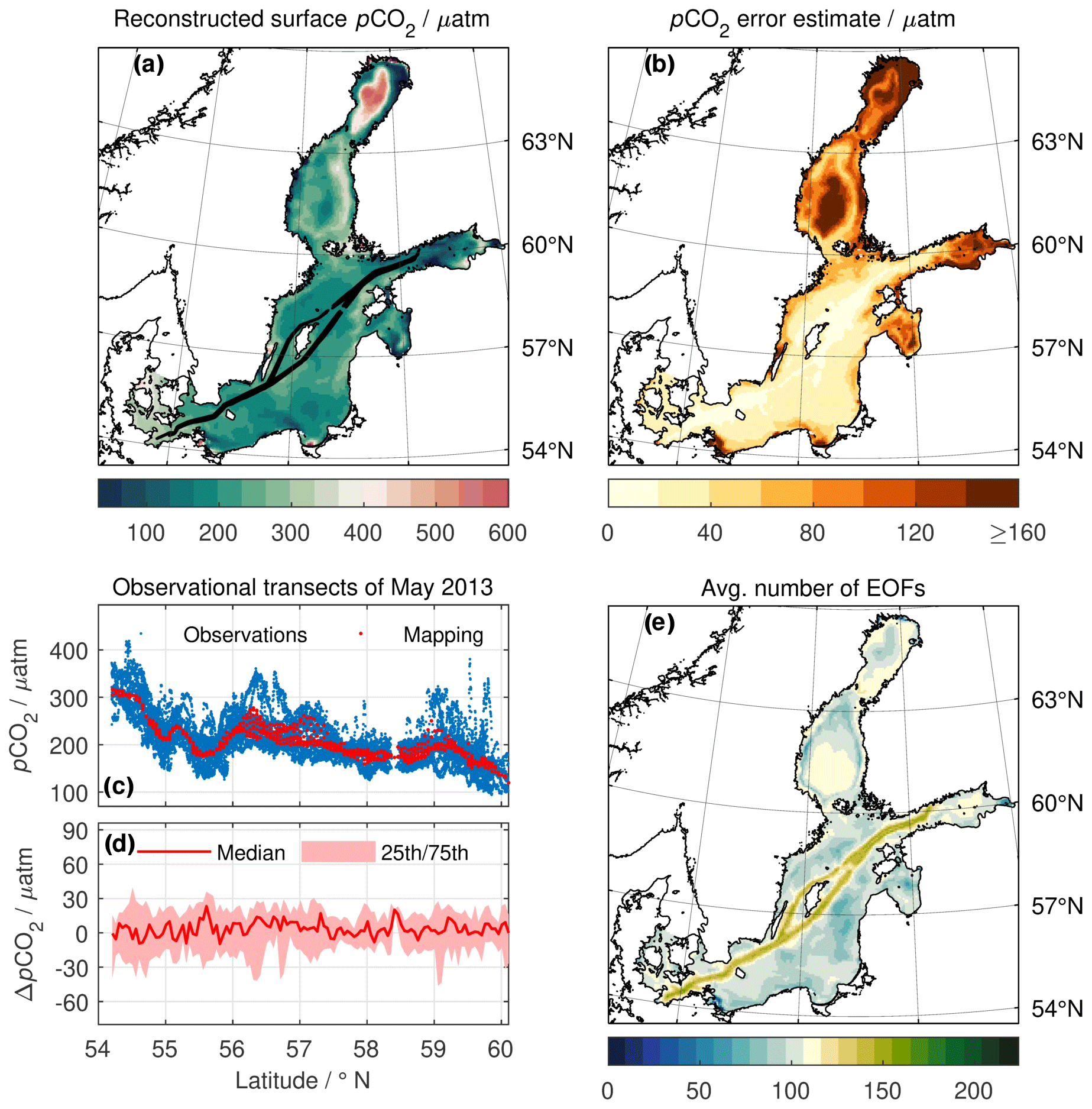
Figure A2 Same as Fig. 3 but without temporally collating the observations to the middle of the month (details in Sect. A7). The general picture of (a) reconstructed pCO₂ x_t,reconstr, (b) pCO₂ error estimate σ_t,reconstr, and (e) average number of patterns $\stackrel{\mathrm{‾}}{\mathit{l}}$ of the reconstruction is comparable to the temporally coherent reconstruction (Fig. 3a, b, g, respectively), but (c) mapped pCO₂ (red) gives only one uniform value throughout the month, and (d) differences to observations are therefore increased (compare Fig. 3e, f).

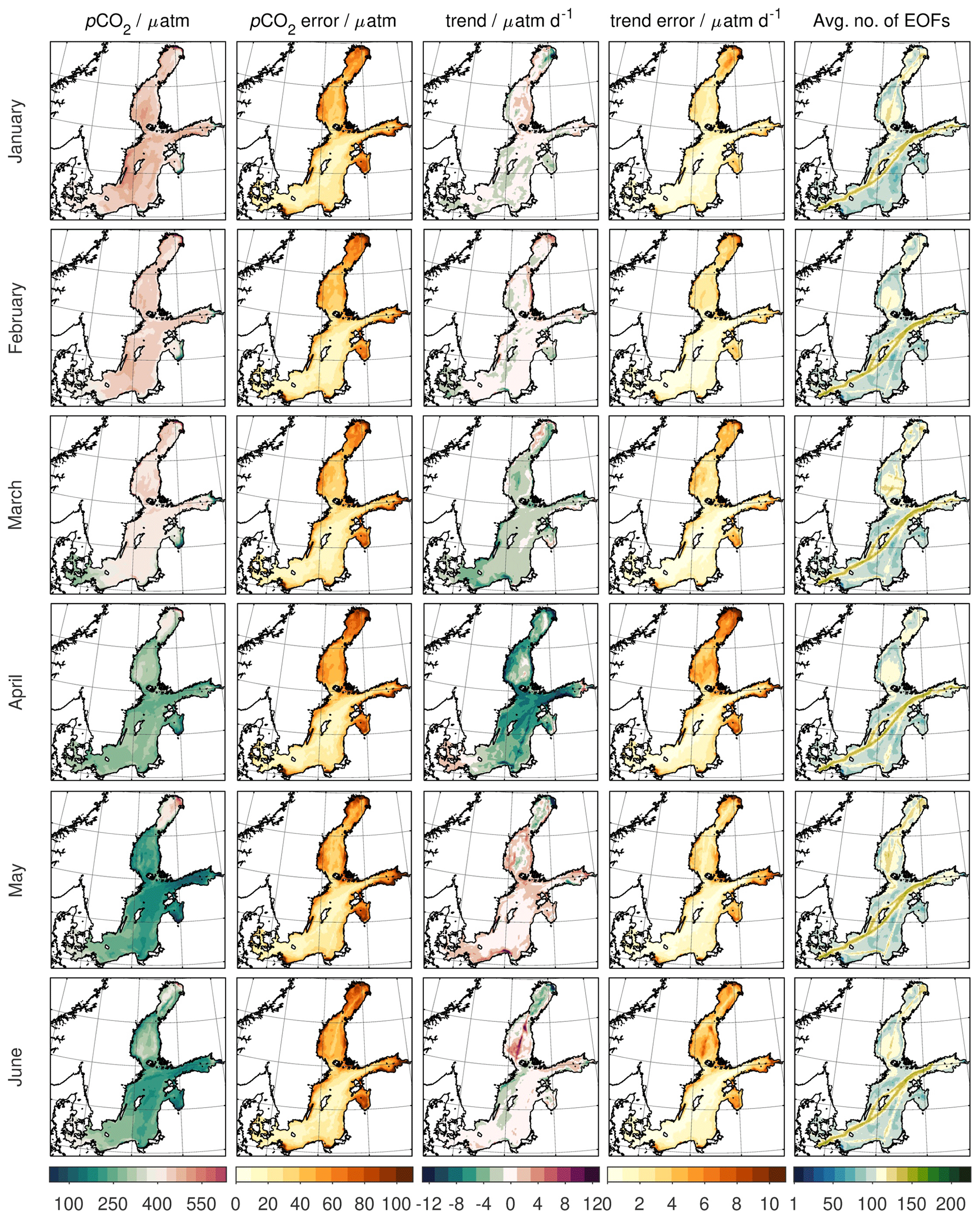
Figure A3 Monthly climatology Y of the surface pCO₂, pCO₂ error estimate, pCO₂ trend, pCO₂ trend error estimate, and average number of EOF patterns in the ensemble (left to right) for the months January–June (top to bottom).

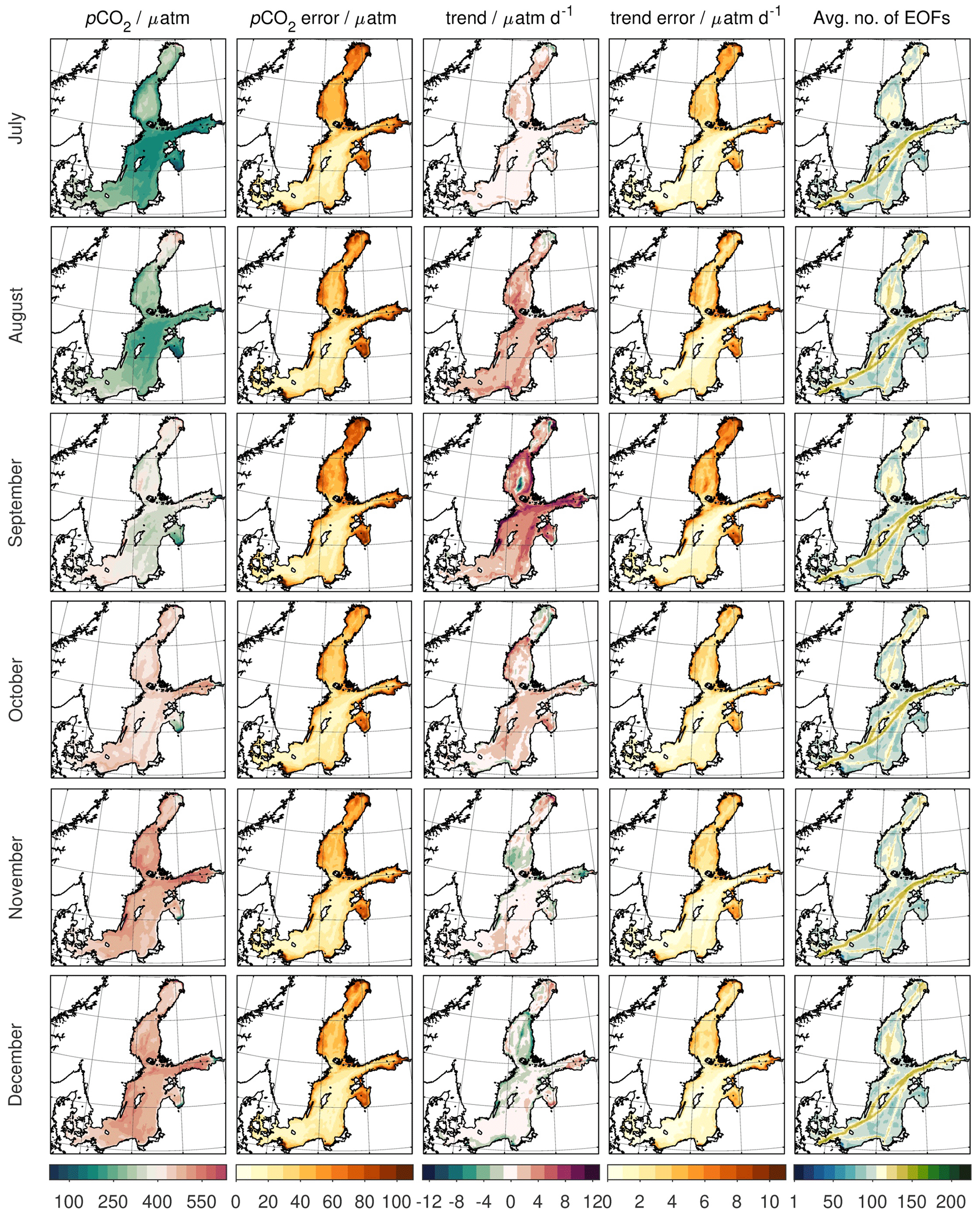
Figure A4 Same as Fig. A3 but for July–December.

We therefore use an ensemble approach over the truncated reconstructions, where we vary l from just 1 mode to l_max modes:

$$\begin{array}{}\text{(A25)}& \stackrel{\mathrm{‾}}{\mathcal{X}}={\displaystyle \frac{{\sum }_{l=\mathrm{1}}^{l_{\max }}{\mathit{w}}_l\cdot {\mathcal{X}}_l}{{\sum }_{l=\mathrm{1}}^{l_{\max }}{\mathit{w}}_l}},\end{array}$$

where the weights w_l (with size m×1) are based on the diagonal elements of P, i.e. the variance ${\mathit{\sigma }}_{P,t}^{\mathrm{2}}$ or mapping uncertainty of the extrapolation:

$$\begin{array}{}\text{(A26)}& {\mathit{w}}_l=\mathrm{1}/{\displaystyle \frac{{\mathit{\sigma }}_{P,t}^{\mathrm{2}}}{{\sum }^m{\mathit{\sigma }}_{P,t}^{\mathrm{2}}}}.\end{array}$$

As the mapped variance diag(P) varies in magnitude with the number of eigenvectors included, the weights w_l for a given number of modes l are normalized by the total variance over all m data points, which gives a normalized spatial weight vector w_l (Eq. A26). For a given spatial data point m, preference is thus given to reconstructions where it is among the better-constrained ones for the given number of modes l.

For 𝓧_l, each using only the first l (≤l_max) eigenvector modes (Eq. A25), we insert the following.

• The reconstructed data vector x_t (from Eq. A9 in truncated form) to yield as $\stackrel{\mathrm{‾}}{\mathcal{X}}$ the ensemble mean $\stackrel{\mathrm{‾}}{{\mathit{x}}_t}$

• The term ${\left(\stackrel{\mathrm{‾}}{{\mathit{x}}_t}-{\mathit{x}}_t\right)}^{\mathrm{2}}$ to yield as $\stackrel{\mathrm{‾}}{\mathcal{X}}$ the biased weighted sample variance about the ensemble mean ${\mathit{\sigma }}_{t,\mathrm{mean}}^{\mathrm{2}}$

• The mapping variance ${\mathit{\sigma }}_{P,t}^{\mathrm{2}}$ (i.e. the diagonal of P; Eq. A23) to yield as $\stackrel{\mathrm{‾}}{\mathcal{X}}$ the remaining mean “large-scale” variance $\stackrel{\mathrm{‾}}{{\mathit{\sigma }}_{P,t}^{\mathrm{2}}}$

• The approximation of the truncated variance ${\mathit{\sigma }}_{P^{\prime },t}^{\mathrm{2}}$ (i.e. the diagonal of P^′; Eq. A24) to yield as $\stackrel{\mathrm{‾}}{\mathcal{X}}$ the mean “small-scale” variance $\stackrel{\mathrm{‾}}{{\mathit{\sigma }}_{P^{\prime },t}^{\mathrm{2}}}$

• The number of modes l itself to yield as $\stackrel{\mathrm{‾}}{\mathcal{X}}$ the average number of modes $\stackrel{\mathrm{‾}}{\mathit{l}}$ used in the reconstruction as a spatial vector of size m×1 each, i.e. on the full spatial domain

The reconstructed data vector x_t,reconstr and the total variance of reconstruction ${\mathit{\sigma }}_{t,\mathrm{reconstr}}^{\mathrm{2}}$ are given by

$$\begin{array}{}\text{(A27)}& {\displaystyle }{\mathit{x}}_{t,\mathrm{reconstr}}& {\displaystyle }=\stackrel{\mathrm{‾}}{{\mathit{x}}_t},\text{(A28)}& {\displaystyle }{\mathit{\sigma }}_{t,\mathrm{reconstr}}^{\mathrm{2}}& {\displaystyle }={\mathit{\sigma }}_{t,\mathrm{mean}}^{\mathrm{2}}+\stackrel{\mathrm{‾}}{{\mathit{\sigma }}_{P,t}^{\mathrm{2}}}+\stackrel{\mathrm{‾}}{{\mathit{\sigma }}_{P^{\prime },t}^{\mathrm{2}}}.\end{array}$$

A7 Temporal coherence

So far, we have considered the observations y_t and the reconstructed data vector x_t to originate and be valid for a given time t, respectively. However, in practice, observations y will spread over a certain time extent Δt, e.g. days for a single SOOP transect to weeks for a basin-covering cruise. If this time extent (e.g. duration of a cruise) is comparable to the timescale of the system's dynamics (e.g. spring surface warming or bloom onset), distortions in the reconstructed fields x_t may occur (Elken et al., 2019) as different “states” of the system could be sampled at different space–time locations.

To collate temporally extended observations into a common synoptic reconstruction without artefacts, Elken et al. (2019) added a linear temporal (short-term) trend for each eigenvector mode to the optimization, thus collating observations made at different observation times t to a common reference time instance t_∘.

To this end,

• the time difference Δt between observation and reference times is introduced:

  $$\begin{array}{}\text{(A29)}& {\displaystyle }\mathbf{\Delta }\mathit{t}=\mathit{t}-t_{\circ }.\end{array}$$

• The sampling operator H_t is extended to not only sample from the eigenvector e_i the value χ corresponding to the observation, but also the value times the time difference, χ⋅Δt, corresponding to a (short-term) time gradient. H_tE thus becomes a matrix of size k×2l.

• The l eigenvalues are replicated with a constant scaling factor, so that Λ becomes a 2l×2l diagonal matrix. That is, both the value (first l eigenvalues) and its time difference (second l eigenvalues times the scaling factor) follow the same eigenvector e_i order and importance, with the scaling factor to determine the balance between both. Based on preliminary tests, we used an empirical scaling between the spatial value pattern and temporal trend pattern of $\mathrm{9}\times {\mathrm{10}}^{-\mathrm{4}}$, equal to a ratio of approximately 1 µatm per 33 d.

• The eigenvalue amplitude vector a_t is doubled in size to 2l×1, where the first l values continue to represent the eigenvectors' e_i amplitudes, while the second l values represent their temporal derivative.

Thus, the system of linear equations (Eqs. A20–A22) becomes a system of 2l equations with 2l unknowns, and the reconstruction (Eq. A9) provides both an extrapolation to the entire spatial domain of m×1 data locations at reference time t_∘ as well as a temporal trend of change in the m×1 data locations at reference time t_∘ (Elken et al., 2019).

Appendix B: Seasonal pCO₂ from value and linear trend climatology by cubic Hermite spline calculation

With a pCO₂ value x and linear pCO₂ trend d given for each month of the climatology, the seasonal evolution of pCO₂ at a given location m can be calculated as a cubic Hermite spline according to

$$\begin{array}{}\text{(B1)}& \begin{array}{rl}{x}_t=& h_{\mathrm{00}}\left(\mathit{\gamma }\right)\cdot x_k+h_{\mathrm{10}}\left(\mathit{\gamma }\right)\cdot d_k\cdot (t_{k+\mathrm{1}}-t_k)+\mathrm{\dots }\\ & h_{\mathrm{01}}\left(\mathit{\gamma }\right)\cdot x_{k+\mathrm{1}}+h_{\mathrm{11}}\left(\mathit{\gamma }\right)\cdot d_{k+\mathrm{1}}\cdot (t_{k+\mathrm{1}}-t_k),\end{array}\end{array}$$

with

$$\begin{array}{}\text{(B2)}& {\displaystyle }{h}_{\mathrm{00}}\left(\mathit{\gamma }\right)=\mathrm{2}{\mathit{\gamma }}^{\mathrm{3}}-\mathrm{3}{\mathit{\gamma }}^{\mathrm{2}}+\mathrm{1},\text{(B3)}& {\displaystyle }{h}_{\mathrm{10}}\left(\mathit{\gamma }\right)={\mathit{\gamma }}^{\mathrm{3}}-\mathrm{2}{\mathit{\gamma }}^{\mathrm{2}}+\mathit{\gamma },\text{(B4)}& {\displaystyle }{h}_{\mathrm{01}}\left(\mathit{\gamma }\right)=-\mathrm{2}{\mathit{\gamma }}^{\mathrm{3}}+\mathrm{3}{\mathit{\gamma }}^{\mathrm{2}},\text{(B5)}& {\displaystyle }{h}_{\mathrm{11}}\left(\mathit{\gamma }\right)={\mathit{\gamma }}^{\mathrm{3}}-{\mathit{\gamma }}^{\mathrm{2}}\text{, and}\text{(B6)}& {\displaystyle }\mathit{\gamma }={\displaystyle \frac{t-t_k}{t_{k+\mathrm{1}}-t_k}}.\end{array}$$

Here, t_k and t_k+1 are the times of the climatological month before and after the time t of interest, and γ gives the normalized time. h(γ) are Hermite basis functions and x_k and x_k+1 as well as d_k and d_k+1 are the associated monthly pCO₂ value and pCO₂ trend, respectively, which determine the seasonal pCO₂ x_t at time t.