Gas exchange velocities (k₆₀₀), gas exchange rates (K₆₀₀), and hydraulic geometries for streams and rivers derived from the NEON Reaeration field and lab collection data product (DP1.20190.001)

Air–water gas exchange is essential to understanding and quantifying many biogeochemical processes in streams and rivers, including greenhouse gas emissions and metabolism. Gas exchange depends on two factors, which are often quantified separately: (1) the air–water concentration gradient of the gas and (2) the gas exchange velocity.  There are fewer measurements of gas exchange velocity compared to concentrations in streams and rivers, which limits accurate characterization of air–water gas exchange (i.e., flux rates). The National Ecological Observatory Network (NEON) conducts SF₆ gas-loss experiments in 22 of their 24 wadeable streams using standardized methods across all experiments and sites, and publishes raw concentration data from these experiments on the NEON data portal. NEON also conducts NaCl injections that can be used to characterize hydraulic geometry at all 24 wadeable streams. These NaCl injections are conducted both as part of the gas-loss experiments and separately. Here, we use these data to estimate gas exchange and water velocity using the reaRate R package. The dataset presented includes estimates of hydraulic parameters, cleaned raw concentration SF₆ tracer-gas data (including removing outliers and failed experiments), estimated SF₆ gas-loss rates, normalized gas exchange velocities (k₆₀₀; m d⁻¹) and normalized depth-dependent gas exchange rates (K₆₀₀; d⁻¹). This dataset provides one of the largest compilations of gas-loss experiments (n=339) in streams to date. This dataset is unique in that it contains gas exchange estimates from repeated experiments in geographically diverse streams across a range of discharges. In addition, this dataset contains information on the hydraulic geometry of all 24 NEON wadeable streams, which will support future research using NEON aquatic data. This dataset is a valuable resource that can be used to explore both within- and across-reach variability in the hydraulic geometry and gas exchange velocity in streams. The data are available at https://doi.org/10.6073/pasta/18dcc1871ee71cf0b69f2ee4082839d0 (Aho et al., 2024), and the reaRate R package code is available at https://doi.org/10.5281/zenodo.12786089 (Cawley et al., 2024).

1 Introduction

Air–water gas exchange contributes to many aquatic processes in streams and rivers, including greenhouse gas emissions (Liu et al., 2022; Rocher-Ros et al., 2023), aquatic metabolism (Aristegi et al., 2009; Hall et al., 2016; Hall and Hotchkiss, 2017), and reoxygenation rates after wastewater discharge (O'Connor and Dobbins, 1958). Despite this importance, gas exchange can be difficult to measure and model (Churchill et al., 1964; Hornberger and Kelly, 1975; Rathbun, 1977; Ulseth et al., 2019). According to Fick's law of diffusion, gas flux across the air–water boundary depends on the concentration gradient of the gas and the gas exchange velocity (k; m d⁻¹):

$$\begin{array}{}\text{(1)}& \text{flux}=k\left({\left[\text{gas}\right]}_{\mathrm{dissolved}}-{\left[\text{gas}\right]}_{\mathrm{equilibrium}}\right),\end{array}$$

where [gas]_dissolved is the concentration of the gas of interest, and [gas]_equilibrium is the concentration of the gas at equilibrium with the atmosphere.

In streams and rivers, measurements of gas concentrations are more readily available than estimates of k; resultantly, estimates of k are often extrapolated from a few measurements. Several methods exist for assessing k, including predictive models (Raymond et al., 2012), models of gas dynamics through time and space in rivers (Appling et al., 2018), and direct measurements with tracers (Hall and Hotchkiss, 2017). Here, k refers to exchange of dissolved gases (i.e., diffusive and bubble-mediated gas transfer) and does not capture ebullitive fluxes. Characterizing k from direct measurement of tracer-gas exchange velocities and modeling based on observed diurnal gas dynamics are likely more accurate for any particular stream or river than more general predictive models (Appling et al., 2018; Hall and Ulseth, 2020; Riley and Dodds, 2013).

Gas exchange velocity is spatiotemporally variable; it is controlled by energy dissipation rate and, therefore, turbulence at the air–water boundary (Zappa et al., 2007). Models that estimate k at broad spatial scales and in low-versus-high gradient streams have found that hydraulic variables (e.g., streambed slope (S; unitless), water velocity (v; m s⁻¹), mean water depth ($\stackrel{\mathrm{‾}}{z}$; m), discharge (Q; L s⁻¹)) are the dominant controls on variation in k (Churchill et al., 1964; O'Connor and Dobbins, 1958; Rathbun, 1977; Raymond et al., 2012). Although similar models for within-reach temporal variability are not widely available, hydrology is expected to control k locally. Existing reach-scale studies have reported different k responses to Q (Genzoli and Hall, 2016; Maurice et al., 2017; McDowell and Johnson, 2018) and point to the importance of quantifying the variable relationships between k and Q on a site-by-site basis. The dataset presented here leverages a unique set of tracer-gas experiments conducted by the National Ecological Observatory Network (NEON) that will allow for assessment of within- and across-reach variability in lotic gas exchange in a wide variety of streams.

Tracer-gas experiments are an approach to estimating k in streams and rivers and involve diffusing an inert tracer gas (e.g., sulfur hexafluoride (SF₆)) at a constant rate at the upstream end of a stream reach and measuring how concentrations decline downstream of the injection point. Often a conservative salt (e.g., sodium chloride (NaCl) or sodium bromide (NaBr)) is also injected with the tracer gas to allow for correction of dilution from hydrologic inflows (referred to as “salt correction” hereafter).

Here, we present a continental-scale dataset of gas exchange rates for wadeable streams derived from NEON data. The substantial processing that was required to estimate gas exchange is described in detail below and archived alongside the dataset. The dataset presented here contains estimates of k₆₀₀, or k normalized to a Schmidt number of 600, and K₆₀₀, which is a depth-corrected rate ($K_{\mathrm{600}}=k_{\mathrm{600}}/\stackrel{\mathrm{‾}}{z}$) used in stream metabolism modeling, for 22 streams and v, $\stackrel{\mathrm{‾}}{z}$, and at-a-station hydraulic geometry for 24 streams (Fig. 1).

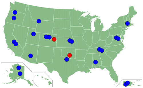
Figure 1 Map of NEON stream sites. Blue symbols indicate sites where NEON conducts full tracer-gas experiments and, thus, where we were able to estimate k₆₀₀, K₆₀₀, v, $\stackrel{\mathrm{‾}}{z}$, and at-a-station hydraulic geometry. Red symbols indicate sites where NEON only conducts NaCl slug injections and, thus, where we were able to calculate v, $\stackrel{\mathrm{‾}}{z}$, and at-a-station hydraulic geometry.

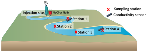
Figure 2 Diagram of a model study reach for NEON tracer-gas experiments. Each ∼500 m study reach comprises an injection site and four downstream sampling stations (Stations 1–4). At the upstream injection site, SF₆ is diffused into the water column with an air stone, and NaCl or NaBr is dripped into the stream. After plateau concentrations are reached at the downstream end of the study reach, injection rates are maintained, and field quintuplicate samples for SF₆ and NaCl or NaBr concentrations are collected at four downstream stations spaced along the study reach. At the upper and lower stations, conductivity sensors are deployed and used to monitor either (1) when NaCl plateau concentrations are reached (for NaCl continuous injections) or (2) when a NaCl “slug” peaks at each station (for NaBr continuous injections). Before each experiment, stream discharge is measured with a flow meter or ADCP, and 30 wetted widths are collected across the study reach. Also, before each injection, background NaCl or NaBr concentrations are collected at all four sampling stations. This diagram uses modified imagery from the University of Maryland Center for Environmental Science Integration and Application Network.

2 Methods

2.1 NEON tracer-gas experiments

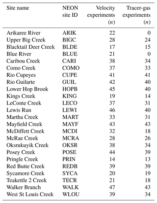
NEON conducts tracer-gas experiments at 22 stream sites, which are distributed across the United States, from Puerto Rico to Alaska (Fig. 1). For information about specific site characteristics, see the NEON website: https://www.neonscience.org/field-sites/explore-field-sites (last access: 2 October 2024). In general, the NEON streams are relatively small; the median watershed size is 11.5 km², while the mean ± standard deviation watershed size is 27.5±58.5 km². Walker Branch (WALK) drains the smallest watershed (1.1 km²) while Sycamore Creek (SYCA), an intermittent, desert stream, drains the largest (280 km²). Therefore, this dataset is only representative of streams and small rivers and not large rivers. These experiments entail continuous injections of SF₆ and a conservative salt tracer (either NaCl or NaBr) at the upstream end of a ≤500 m stream reach (Fig. 2). NEON uses SF₆ because it does not occur naturally, is not biologically or chemically reactive, and can be detected at low concentrations (Cole and Caraco, 1998; Ho et al., 2011; Maurice et al., 2017; Wanninkhof et al., 1985); although used in very small amounts in these experiments, SF₆ is a potent greenhouse gas, and tracer-gas experiments are ceasing at sites with sufficient hydrologic coverage. When NaBr is used as the salt tracer, an additional NaCl “slug” injection is performed, which allows for the subsequent calculation of v and the derivation of $\stackrel{\mathrm{‾}}{z}$ from paired Q measurements (via flowmeter or acoustic Doppler current profiler, ADCP) and wetted width measurements taken at 30 points along the study reach. Before the injection, NaCl or NaBr is collected at each of the four stations along the study reach; these data can later be used to correct NaCl or NaBr concentrations during the injection for background conditions. Once conductivity during the injection either reaches a plateau (for constant-rate NaCl injections) or returns to background levels (for NaCl slug injections) at the most downstream station, five replicate SF₆ and NaCl or NaBr samples are collected at each of the four stations located along the study reach. Samples for SF₆ are collected via headspace equilibration in 60 mL syringes, stored in gas-tight evacuated vials (12 mL, Exetainer), and run on a gas chromatograph with an electron capture detector (ECD). Samples for NaCl and NaBr are filtered to 0.7 µm, collected in 60 mL HDPE bottles, and run on an ion chromatograph. In addition, high-frequency (0.1 Hz) sensors are deployed to monitor NaCl conductivity at the upstream and downstream end of the study reach (Fig. 2). NEON publishes SF₆ mixing ratios, NaCl and NaBr concentrations, wetted width data, and conductivity time series from these experiments as the Reaeration field and lab collection data product, DP1.20190.001 (NEON, 2024b), and measurements of Q in the Discharge field collection data product, DP1.20048.001 (NEON, 2024a). More detailed information on NEON's data collection procedures can be found on their website, http://www.neonscience.org (last access: 2 October 2024).

NEON has conducted tracer-gas experiments 6–10 times per year for 6–8 years at all 22 sites to capture a range of discharge conditions. Presently, tracer-gas experiments are ceasing at sites with sufficient hydrograph coverage (https://www.neonscience.org/impact/observatory-blog/protocol-change-reaeration-field-and-lab-collection-dp120190001, last access: 2 October 2024). However, NaCl slug injections will continue to be performed quarterly to collect high-frequency conductivity time-series data that allow for the calculation of v and the derivation of $\stackrel{\mathrm{‾}}{z}$ from paired Q and wetted-width measurements. Similarly, NaCl slug injections are and will continue to be conducted for the two sites where tracer-gas experiments are not collected (Blue River (BLUE), where wide channel widths and high discharges make tracer-gas studies challenging, and Arikaree River (ARIK), where long travel times make tracer-gas studies infeasible).

The dataset presented here represents substantial processing of these published data (i.e., SF₆ mixing ratios, NaCl and NaBr concentrations, conductivity time series, wetted widths, and measurements of Q) to estimate k₆₀₀ or K₆₀₀ using the reaRate R package (Cawley et al., 2024). In addition, this dataset contains estimates of v from NaCl injections, which, as mentioned above, are performed both during tracer-gas experiments and at quarterly intervals at sites where tracer-gas experiments are not conducted or have ceased. Along with the paired Q measurement and the average wetted width for the study reach ($\stackrel{\mathrm{‾}}{w}$; m), the estimate of v was used to derive $\stackrel{\mathrm{‾}}{z}$. The dataset presented here contains estimates of v and $\stackrel{\mathrm{‾}}{z}$ and at-a-station hydraulic geometry for all 24 NEON wadeable streams. This dataset provides a large compilation of direct measurements of tracer-gas experiments and at-a-station hydraulic geometry in small streams across the United States.

2.2 reaRate R package

The data processing pipeline described below uses the reaRate R package (Cawley et al., 2024). The package estimates k₆₀₀ and K₆₀₀ from data available on the NEON data portal. The package works by fitting an exponential, first-order decay function to the observed longitudinal decline in published SF₆ concentrations and solving for the longitudinal tracer-gas-loss rate (K_d; m⁻¹):

$$\begin{array}{}\text{(2)}& C_x=C_{\mathrm{0}}{e}^{-K_{\mathrm{d}}x},\end{array}$$

where C₀ and C_x are tracer-gas concentrations at the top of the study reach and at a downstream point x, respectively, and K_d is the average distance traveled by an SF₆ molecule before it is emitted to the atmosphere. For sites where lateral inflows (e.g., groundwater inputs, overland flow, tributaries) appear to dilute SF₆ concentrations, the ratio of SF₆ to NaCl or NaBr is used to calculate a salt-corrected K_d value. The K_d values can then be converted to the gas exchange velocity for the tracer gas (e.g., $k_{{\mathrm{SF}}_{\mathrm{6}}}$; m d⁻¹):

$$\begin{array}{}\text{(3)}& k_{{\mathrm{SF}}_{\mathrm{6}}}=\stackrel{\mathrm{‾}}{z}\mathit{\nu }{K}_{\mathrm{d}}.\end{array}$$

This gas-specific k can be normalized to k₆₀₀ using a Schmidt number of 600:

$$\begin{array}{}\text{(4)}& k_{\mathrm{600}}=k_{{\mathrm{SF}}_{\mathrm{6}}}{\left({\displaystyle \frac{\mathrm{600}}{{\mathit{Sc}}_{{\mathrm{SF}}_{\mathrm{6}}}}}\right)}^{-n},\end{array}$$

where n is the Schmidt number exponent (0.5 for flowing waters), and ${\mathit{Sc}}_{{\mathrm{SF}}_{\mathrm{6}}}$ is the temperature-dependent Schmidt number for SF₆ at water temperature T in degrees Celsius (Jähne et al., 1987; Raymond et al., 2012; Wanninkhof, 1992):

$$\begin{array}{}\text{(5)}& {\mathit{Sc}}_{{\mathrm{SF}}_{\mathrm{6}}}=\mathrm{3255.3}-\mathrm{217.13}T+\mathrm{6.8370}{T}^{\mathrm{2}}-\mathrm{0.086070}{T}^{\mathrm{3}}.\end{array}$$

Reporting estimates of k₆₀₀ is common; it allows for comparisons with existing work and can be scaled to other gases, including CO₂ and O₂, using the same approach as in Eq. (4) with gas-specific, temperature-dependent Schmidt numbers:

$$\begin{array}{}\text{(6)}& k_{\mathrm{gas}}=k_{\mathrm{600}}{\left({\displaystyle \frac{{\mathit{Sc}}_{\mathrm{gas}}}{\mathrm{600}}}\right)}^{-\frac{\mathrm{1}}{\mathrm{2}}}.\end{array}$$

Some applications (e.g., metabolism, reoxygenation rates) explicitly include water depth in their modeling frameworks and thus require a depth-dependent gas exchange rate (K; d⁻¹). In these cases, a normalized gas exchange rate (K₆₀₀) can be used and is related to k₆₀₀ by dividing by $\stackrel{\mathrm{‾}}{z}$ for the upstream reach corresponding to a length of at least $\frac{\mathrm{1}}{K_{\mathrm{d}}}$ . Using the same scaling relationships shown in Eqs. (3) and (5), K₆₀₀ can be converted to gas-specific K_gas estimates.

The reaRate package uses NaCl breakthrough curves (i.e., from either continuous injection or slug injections) to estimate the travel time between the upstream and downstream stations and then calculates v as the distance between stations divided by the travel time. Using the continuity equation, $\stackrel{\mathrm{‾}}{z}$ is calculated by dividing Q by v and $\stackrel{\mathrm{‾}}{w}$. Finally, $k_{{\mathrm{SF}}_{\mathrm{6}}}$ and $K_{{\mathrm{SF}}_{\mathrm{6}}}$ are calculated from K_d, v, and $\stackrel{\mathrm{‾}}{z}$ (Eq. 3) and then normalized to k₆₀₀ and K₆₀₀ (Eq. 4). The reaRate package includes two approaches to estimate k₆₀₀ and K₆₀₀: an un-pooled frequentist approach and a partially pooled Bayesian approach, both of which are described in more detail below. Implementation of the package and all processing described below were conducted in R 4.2.3 (R Core Team, 2023). More information about the package, including details about the individual functions and a processing pipeline, is provided in Sect. 2.3.

Figure 3 Overview of data processing to estimate k₆₀₀ and K₆₀₀ from NEON tracer-gas experiments.

2.3 Data processing

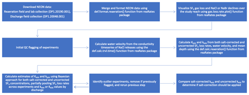
Substantial processing was required to estimate k₆₀₀ and K₆₀₀ from the NEON data (Fig. 3). All data used were downloaded from the NEON data portal. Downloads consisted of two NEON data products: Reaeration field and lab collection (DP1.20190.001) and Discharge field collection (DP1.20048.001). Data were from RELEASE-2023, in addition to nine experiments that were provisional but are now included in RELEASE-2024 (NEON, 2023a, b, 2024a, b). On a site-by-site basis, data were merged and formatted using the def.format.reaeration() function from the reaRate R package. This function compiles variables from across the downloaded data into a single data frame. These variables include Q, $\stackrel{\mathrm{‾}}{w}$, water temperature, station location as a distance downstream from the injection point, and SF₆ and NaCl or NaBr concentrations for each station during the experiment. The function also applies a salt correction to the SF₆ data (e.g., SF₆ concentration divided by background-corrected NaCl or NaBr concentrations). The function removes outliers (points more extreme than 1.5×IQR below and above the first and third quartile, respectively) from the quintuplet SF₆ and NaCl or NaBr concentrations for each station, calculates the mean and standard deviation SF₆ and NaCl or NaBr concentration for each station, and flags stations as “unmixed” when the coefficient of variation ($\text{CV}=\frac{\text{SD}}{\text{mean}}$) of the replicate SF₆ and NaCl or NaBr concentrations is greater than 10 %.

Table 1 Sites and number of experiments.

Next, SF₆ and NaCl or NaBr declines were visualized and quantified for each experiment and initial quality control flags were assigned. The gas.loss.rate.plot() function from the reaRate package was used to visualize and calculate both salt-corrected and uncorrected longitudinal gas-loss rates over the length of the study reach (K_d). For the sites requiring a salt correction to account for lateral inflows, mean SF₆ mixing ratios at each station were first divided by mean background-corrected NaCl or NaBr concentration for the corresponding station. Station-specific outliers (i.e., values more extreme than first quartile $-\mathrm{1.5}\times \text{IQR}$ and third quartile $+\mathrm{1.5}\times \text{IQR}$) were removed. SF₆ concentrations were then log-normalized, and K_d was calculated from the resulting linear decline. A quality control flag was assigned to an individual experiment if any of the following criteria applied:

• Visually, the SF₆ gas-loss rate over the entire study reach was unduly affected by anomalous SF₆ concentrations (potentially indicating contamination, leaked vials, or analytical error).

• SF₆, NaCl, or NaBr concentrations increased in a downstream direction between any of the stations (likely indicating incomplete mixing in the water column).

• The salt-corrected K_d was larger than the uncorrected K_d (a salt correction should correct for overestimation due to lateral inflows, with the reverse potentially indicating contamination or analytical error).

For each experiment, v was calculated from the conductivity time series using the def.calc.trvl.time() function. The function requires that the user manually selects points bracketing either the rising limb (for constant rate injections) or the peak concentration (for slug injections). From within the user-selected bracket, the def.calc.trvl.time() function smooths the data using a loess function and then identifies the peak of the breakthrough by finding either where the first derivative is 0 (for a slug injection) or where it is at its maximum (for a constant rate injection). This function then calculates the breakthrough travel time between the two stations and uses the distance between stations to calculate v. Site-specific relationships between v and Q were visualized in log–log space, and any anomalous values were reprocessed with the def.calc.trvl.time() to confirm that the user-selected bracketing allowed the function to pick the correct points on the time series. Finally, $\stackrel{\mathrm{‾}}{z}$ was calculated using the def.calc.trvl.time() function, which divides Q by v and $\stackrel{\mathrm{‾}}{w}$.

Two separate approaches were used to estimate k₆₀₀ or K₆₀₀ values from the formatted data. The first approach used the def.calc.reaeration() function to multiply K_d for each individual experiment by the corresponding v and $\stackrel{\mathrm{‾}}{z}$ values (Eq. 3) to estimate $k_{{\mathrm{SF}}_{\mathrm{6}}}$, which were then converted to k₆₀₀ (Eq. 4). The resulting k₆₀₀ estimates were converted to K₆₀₀ by dividing by water depth. This approach is subsequently referred to as the un-pooled, frequentist approach and is included in this data descriptor because it represents the current, prevailing approach for processing this type of data, is straightforward to implement, and represents the output of the def.calc.reaeration() function included in the reaRate package.

The second approach used Bayesian multilevel models that pooled experiments from the same site across releases. The models, coded in the Stan probabilistic programming language, used for this approach are also included in the reaRate package. A Bayesian approach provides flexibility in specifying models that consider repeat experiments at a site and current theory surrounding gas exchange. Bayesian inference allowed partial pooling of k₆₀₀ estimates across releases in any one stream. Partial pooling reduces the error in any one estimate of k₆₀₀ and shrinks all k₆₀₀ estimates to the site-level mean (as conditioned on discharge) if error in measuring SF₆, NaCl, and/or NaBr is high.

The Bayesian approach included error at two levels. First, the models pooled k₆₀₀ estimates across releases from the same site to estimate K_d from normalized SF₆ concentrations (both salt-corrected and uncorrected). For this step, the relationship between the SF₆ loss rate and the product of K_d and reach length was assigned a prior normal distribution with a normally distributed sigma (0, 0.2) and intercept (0, 0.1). We fully pooled the intercept with a strong prior near 0 because all SF₆ concentrations (i.e., measurements from Stations 1–4) were normalized to the SF₆ concentration at Station 1; this approach means that the intercept should be near 1, or 0 when logged. Thus, the model fit can be described as variable-slope, fixed-intercept linear regression. Second, the models pooled the estimates of k₆₀₀ and K₆₀₀ by Q, using linear relationships between Q and k₆₀₀ or K₆₀₀. Priors were assigned for both the slope and the intercept based on predictions from an existing scaling model (Eq. 4 in Raymond et al., 2012). These priors were given large variances when possible (i.e., 10 for the intercept and 1 for the slope) to allow for divergence from the model predictions. However, at sites with a limited number of experiments (e.g., Pringle Creek, PRIN, and Kings Creek, KING), we used smaller variances to allow the model to converge. The site-specific priors used are listed in Table S1.

The two levels described can be referred to as a within-release model and an among-release model. The within-release model was a log-transformed (base e) exponential model. We log-transformed the model because SF₆ is always positive (ambient = 0) and because errors in the measurement of SF₆ can scale with the magnitude of the concentration.

$$\log \left(S_{i,j}\right)=\log \left(S_{\mathrm{0}}\right)-K_{D,j}{x}_{i,j}+{\mathit{\epsilon }}_{i,j}$$

and

$${\mathit{\epsilon }}_{i,j}\sim \text{normal}\left(\mathrm{0},{\mathit{\sigma }}_{\mathrm{release}}\right),$$

where S_i,j is the SF₆ concentration normalized to the concentration at Station 1 for any one release (sample i in release j), S₀ is the normalized SF₆ concentration at Station 1, x_i,j is the distance downstream to which the normalized concentration corresponds, and ε_i,j is a normally distributed random variable with μ=0 and SD=σ_release. We then converted K_D,j to gas exchange velocity $k_{{\mathrm{SF}}_{\mathrm{6}},j}$ using Eq. (3) and normalized to k_600,j using Eq. (4). The among-release model included a linear model predicting the parameter k_600,j as a linear function of discharge:

$$\log \left(k_{\mathrm{600},j}\right)=a+b\times \log \left(Q_j\right)+{\mathit{\epsilon }}_j$$

and

$${\mathit{\epsilon }}_j\sim \text{normal}\left(\mathrm{0},{\mathit{\sigma }}_{\mathrm{stream}}\right),$$

where a and b are the intercept and slope parameters of a model regressing log (k_600,j) and log (Q_j), where Q_j is the discharge during any one release and σ_stream is the residual variation. We also fit linear second-level models with log (K_600,j), where K_600,j is the per-time gas exchange rate.

We fit models using Stan in the RStan package in R (Stan Development Team, 2023). The models were run for at least 5000 iterations over four chains. Models were assessed according to the number of divergent transitions, the effective sample size (ESS) for each estimated parameter (>1000), and posterior predictive checks with the ShinyStan R package (Gabry et al., 2023). In addition, the model fits for each experiment were visually assessed (Figs. S1–S2). Finally, the median estimates for k₆₀₀ and K₆₀₀ were visualized in log(k₆₀₀)–log(Q) or log(K₆₀₀)–log(Q) space, respectively, along with 1000 Markov chain–Monte Carlo (MCMC) estimates of the log(k₆₀₀)–log(Q) or log(K₆₀₀)–log(Q) relationship, respectively. If an estimate of k₆₀₀ and K₆₀₀ fell outside the overall Q relationship and if that experiment's model fits showed signs of being unduly influenced by unrealistic gas-loss patterns (e.g., very little decline indicating the study reach was too short, an abrupt decline indicating improper mixing), the experiment was assessed for the QC flags described above. If a QC flag had previously been assigned, then that experiment was removed (e.g., it was identified as an outlier and could be attributed to experimental error), and the model was rerun without that experiment.

2.4 Recommended estimates

The processing pipeline outlined above in Sect. 2.3 resulted in both un-pooled frequentist and Bayesian estimates of k₆₀₀ and K₆₀₀, both with and without salt corrections. We include outputs from all four approaches in the dataset for completeness and to allow future users to decide which estimates best fit their needs and to compare the two approaches. The complete dataset is available in the gasExchange_ds_v2.csv file (Aho et al., 2024).

During data processing, we found that the NaCl and NaBr concentration data also could introduce errors and uncertainties into our estimates of k₆₀₀ and K₆₀₀. For instance, background concentrations at a single station were occasionally so high that contamination was the likely explanation. Further, sometimes samples taken during the constant-rate injection could vary across the reach in unpredictable ways (e.g., increases across the reach, random peaks along the reach instead of the expected stable, declining concentrations), which was likely the result of incomplete mixing with the water column. In many cases, the quality of the salt-corrected SF₆ data precluded Bayesian-model convergence. Through assessing the gas-loss plots and salt concentration declines for all experiments and the failures to produce model convergence for salt-corrected data, we determined that salt corrections had the strong potential to either introduce errors into or preclude estimates of k₆₀₀ and K₆₀₀. Therefore, we suggest only using salt-corrected data when clearly necessary (e.g., obvious lateral inflow) and possible in terms of data quality and model convergence. We determined that salt correction was important for five sites: Como Creek (COMO), Rio Cupeyes (CUPE), Rio Yahuecas (GUIL), Martha Creek (MART), and Walker Branch (WALK). Notably, several of these sites have lateral inflows within the study reach under certain hydrologic conditions, which explains the necessity for the salt correction. For completeness, our dataset includes estimates for both uncorrected and salt-corrected k₆₀₀ and K₆₀₀ when a salt correction is possible.

In addition to the complete dataset of all estimates (i.e., estimates from both frequentist and Bayesian approaches for both uncorrected and salt-corrected data), we also include a curated dataset of recommended estimates of k₆₀₀ and K₆₀₀. These recommended values are called “best_k600_mPerDay” and “best_K600_perDay” in the gasExchange_ds_v2.csv file. In all cases, the curated selection uses the Bayesian estimates because pooling across experiments and the use of informative priors resulted in more meaningful estimates than the non-Bayesian approach. The choice of whether we recommend an uncorrected or salt-corrected estimate stems from examining the relationships between uncorrected or salt-corrected estimates (Fig. S3).

3 Data description

3.1 Hydraulics

Our processing pipeline included calculating hydraulic parameters (v and $\stackrel{\mathrm{‾}}{z}$) for each of the NaCl injections and measurements of Q and $\stackrel{\mathrm{‾}}{w}$. These variables (v, $\stackrel{\mathrm{‾}}{z}$, Q, and $\stackrel{\mathrm{‾}}{w}$) for each NaCl release are available in the hydraulics_v2.csv file (Aho et al., 2024). Here, we present those data in terms of at-a-station hydraulic geometries, which are commonly used to quantify reach-specific relationships between Q and $\stackrel{\mathrm{‾}}{w}$, $\stackrel{\mathrm{‾}}{z}$, and v (Leopold and Maddock, 1953):

$$\begin{array}{}\text{(7)}& {\displaystyle }\stackrel{\mathrm{‾}}{w}=a{Q}^b\text{(8)}& {\displaystyle }\stackrel{\mathrm{‾}}{z}=c{Q}^f\text{(9)}& {\displaystyle }v=k{Q}^m.\end{array}$$

In log–log space, these exponential relationships become linear relationships (e.g., $\stackrel{\mathrm{‾}}{w}=a{Q}^b$ becomes $\log \left(\stackrel{\mathrm{‾}}{w}\right)=\log \left(a\right)+b\times \log \left(Q\right)$), where the exponent is the slope log-linear relationship. Future users of NEON data can use these relationships along with discharge values from either the Continuous discharge data product (DP4.00130.001) or the Discharge field collection (DP1.20048.001) to approximate $\stackrel{\mathrm{‾}}{w}$, $\stackrel{\mathrm{‾}}{z}$, and v for NEON streams.

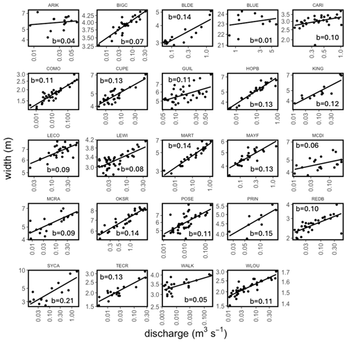
Figure 4 At-a-station hydraulic geometries for the relationship between Q and w. The exponent b of the power law relationship $\stackrel{\mathrm{‾}}{w}=a{Q}^b$ is the linear slope of the relationship in log–log space and is denoted on each subplot.

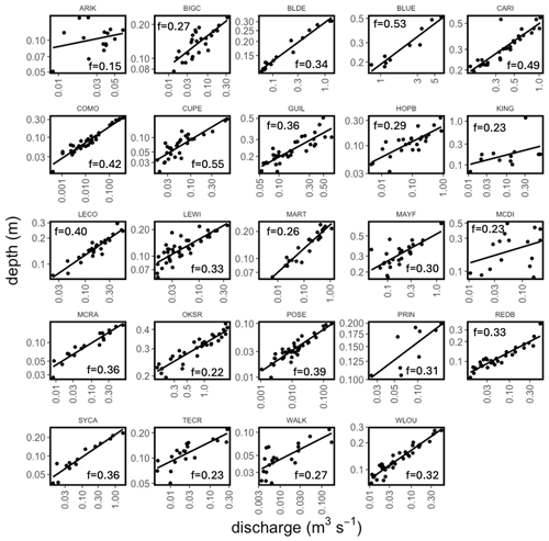
Figure 5 At-a-station hydraulic geometries for the relationship between Q and $\stackrel{\mathrm{‾}}{z}$. The exponent f of the power law relationship $\stackrel{\mathrm{‾}}{z}=c{Q}^f$ is the linear slope of the relationship in log–log space and is denoted on each subplot.

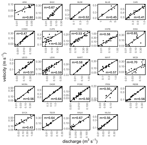
Figure 6 At-a-station hydraulic geometries for the relationship between Q and v. The exponent of the power law relationship v=kQ^m is the linear slope of the relationship in log–log space and is denoted on each subplot.

Table 2 Coefficients and exponents from at-a-station hydraulic geometries. The 95 % confidence intervals for each coefficient and exponents are shown. In addition, the R² values from the log-linear relationships are also presented.

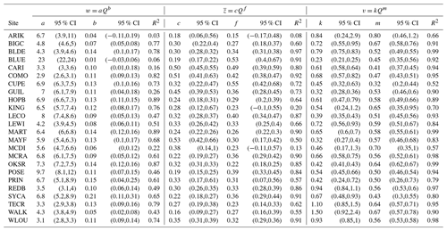
The hydraulic relationships are illustrated (Figs. 4–6, Table 2). These geometries leverage field measurements of $\stackrel{\mathrm{‾}}{w}$ (n=783) and Q (n=601), estimates of v (n=618) from NaCl injections, and estimates of $\stackrel{\mathrm{‾}}{z}$ (n=581) calculated from $Q/v\stackrel{\mathrm{‾}}{w}$. The timing of these measurements is denoted on site-specific hydrographs for each site (Fig. S4), and their coverage of site-specific Q ranges is illustrated on flow duration curves (Fig. S5). In general, $\stackrel{\mathrm{‾}}{z}$–Q and v–Q relationships were the strongest, with all but three relationships having R²>0.5 and relatively narrow 95 % confidence intervals around the coefficients from these relationships (Table 2). The $\stackrel{\mathrm{‾}}{w}$–Q relationships are the weakest; 9 of the 24 sites have R²<0.5 and large 95 % confidence intervals (Table 2). The $\stackrel{\mathrm{‾}}{w}$–Q relationships may be weaker because our width estimates represent an average of 30 measurements across the ∼500 m study reach. It is possible that this across-reach averaging contributes to the weaker relationships with Q and that perhaps the relationships would be stronger if the measurement was only taken at the same location as the Q measurement. However, this single-point approach would be less compatible with v measured of the entire reach and would alter the resulting calculations of $\stackrel{\mathrm{‾}}{z}$.

We assess the quality of our hydraulic parameters by examining the product of the constants ($a\times c\times k$) and sum of the exponents ($b+f+m$) for unity on a site-by-site basis. These unity relationships stem from the fact that Q=wzv (Leopold and Maddock, 1953). The products of the constants ranged from 0.93 to 1.04 and averaged 1.00; the site-specific sum of the exponents ranged from 0.96 to 1.01 and averaged 1.00. There was one instance where the product of the constants deviated more than 5 % from unity (0.93, PRIN). Pringle Creek (PRIN) is a semi-arid, intermittent stream in Texas, and so the deviation from unity may stem from logistical difficulties in measuring low and non-perennial stream flows (Seybold et al., 2023; Shanafield et al., 2021). However, the remainder of the sites had both products of constants and sums of exponents within 5 % of unity.

We assess the representativeness of our hydraulic parameters through comparison to literature values for the exponents. Previous studies have shown large ranges for all three exponents, with ranges spanning 0–0.6 for b, 0–0.8 for f, and 0–0.8 for m (Park, 1977; Rhodes, 1977). In addition, exponents have not been shown to vary predictably with region or climate (Park, 1977) but rather with channel geometry (Ferguson, 1986). Our parameters fall within published ranges, and our average values for each exponent (b=0.11, f=0.33, m=0.56) are similar to averages in other studies that span many streams (b=0.14, f=0.30; Morel et al., 2020; b=0.12, f=0.37, m=0.51; Dingman and Afshari, 2018). In sum, the hydraulics dataset and associated hydraulic-geometry relationships presented here can be used to characterize $\stackrel{\mathrm{‾}}{w}$, $\stackrel{\mathrm{‾}}{z}$, and v for NEON streams.

3.2 k₆₀₀ and K₆₀₀ estimates

As described above, k₆₀₀ was estimated in two ways: (1) via an unpooled frequentist approach using the def.calc.reaeration() function to estimate k₆₀₀ independently for each experiment and (2) via a partially pooled Bayesian approach that partially pooled experiments from the same site according to Q. Both approaches were attempted for raw SF₆ concentrations and salt-corrected SF₆ concentrations. Salt-corrected SF₆ concentrations are only recommended for the five sites mentioned above (COMO, CUPE, GUIL, MART, WALK). All estimates are available in the gasExchange_ds_v2.csv file (Aho et al., 2024).

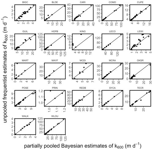
Figure 7 Comparison of partially pooled Bayesian and unpooled frequentist estimates of k₆₀₀. Black 1:1 lines overlay the points for reference.

The relationship between the partially pooled and unpooled estimates (with salt correction when appropriate) is shown in Fig. 7. Any points falling above the 1:1 line are instances when partial pooling resulted in a lower estimate than no pooling, and vice versa. Overall, there are instances where partially pooled estimates are both higher and lower than un-pooled estimates, suggesting that partial pooling successfully regularized estimates. This shrinkage is more obvious when both estimates are plotted against Q (Fig. 8). We made recommendations (best_k600_mPerDay and best_K600_perDay in the gasExchange_ds_v2.csv) of which estimates to use; this curated dataset includes only Bayesian estimates, and a salt correction was only recommended for the five sites where it was possible and necessary.

Table 3 Mean, standard deviation (SD), minimum, maximum, and count for k₆₀₀ (m d⁻¹) and K₆₀₀ (d⁻¹) estimates by site.

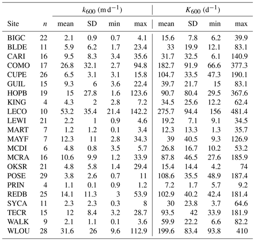
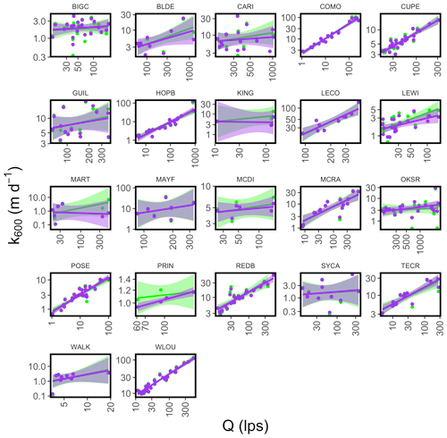
Figure 8 Relationship between Q and partially pooled Bayesian and unpooled frequentist estimates of k₆₀₀. The unpooled estimates are shown in green, with a green regression line with 95 % confidence intervals, while the partially pooled estimates are shown in purple, with a purple regression line with 95 % confidence intervals.

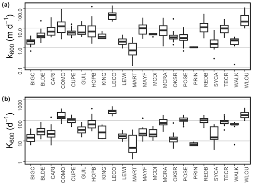
Figure 9 Box plots of the test estimates of (a) k₆₀₀ and (b) K₆₀₀ by site. Boxes represent the median and interquartile range (IQR), whiskers mark the lesser of first (third) quartile − (+) 1.5×IQR or minimum/maximum, and points denote outliers more extreme than first (third) quartile − (+) 1.5×IQR.

There are 339 estimates of k₆₀₀ and K₆₀₀ included in our recommended dataset (Fig. 9, Table 3) that span large Q ranges at each site (Figs. S4–S5). The number of estimates per site ranges from 4 (Kings Creek (KING) and Pringle Creek (PRIN)) to 29 (Posey Creek (POSE)). The issueLog.csv file documents the reason that 340 experiments did not successfully produce gas exchange estimates. These reasons are grouped into broad categories and summarized in Table S2. It is possible that some of the experiments that we removed could produce an estimate of k₆₀₀ and K₆₀₀ (e.g., if there was incomplete mixing at the first station, one could remove this station and only estimate k₆₀₀ and K₆₀₀ for Stations 2–4). However, this type of selective cleaning would have resulted in less comparable estimates (e.g., changing the length of the study reach), so we chose to include only the most comparable and high-quality experiments in this dataset.

The values for recommended estimates of k₆₀₀ ranged from 0.1 to 142 m d⁻¹. LeConte Creek (LECO) had the highest mean k₆₀₀ (mean ± SD: 53±35 m d⁻¹), while Pringle Creek (PRIN) had the lowest mean k₆₀₀ (mean ± SD: 1.1±0.1 m d⁻¹). Lower Hop Brook (HOPB) had the widest spread of k₆₀₀ values, with estimates ranging almost 2 orders of magnitude (1.5–124 m d⁻¹), while Pringle Creek (PRIN) had the smallest spread, with estimates only ranging from 0.9 to 1.2 m d⁻¹. The values for recommended estimates of K₆₀₀ range from 1.3 to 481 d⁻¹. Like for k₆₀₀, LeConte Creek (LECO) had the highest mean K₆₀₀ (mean ± SD: 276±94 d⁻¹), while Pringle Creek (PRIN) had the lowest mean K₆₀₀ (mean ± SD: 7.0±1.9 d⁻¹). Also, Lower Hop Brook (HOPB) had the widest spread of K₆₀₀ values, with estimates ranging from 30 to 368 d⁻¹, while Pringle Creek (PRIN) had the smallest spread, with estimates ranging from 5.3 to 9.3 d⁻¹. These ranges, in part, reflect the various ranges of Q captured at each site (Table S3). HOPB was among the sites with the largest range of Q captured, while PRIN was among the sites with the smallest Q range captured (Table S3). Overall, this large compilation of k₆₀₀ and K₆₀₀ estimates indicates high variability both across and within sites.

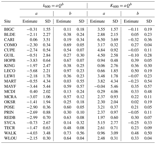
Finally, to allow future users to scale k₆₀₀ and K₆₀₀ with Q, we include both the slope and intercept for the k₆₀₀–Q and K₆₀₀–Q relationships (Table 4) and the stanfit objects for the Bayesian models (“Other Entities” in the data release). The slope and intercept will allow future users a straightforward way to scale k₆₀₀ or K₆₀₀ as a function of Q at each site. The stanfit objects, on the other hand, will allow future users to sample from the posterior distribution of slope and intercept to assess uncertainty in the scaling relationships.

Table 4 Coefficients and exponents for k₆₀₀–Q and K₆₀₀–Q relationships. Estimates and standard deviations (SD) are given.

4 Code and data availability

The reaRate R package is available at https://doi.org/10.5281/zenodo.12786089 (Cawley et al., 2024). The dataset of hydraulic parameters and gas exchange estimates is available from the Environmental Data Initiative: https://doi.org/10.6073/pasta/18dcc1871ee71cf0b69f2ee408 2839d0 (Aho et al., 2024).

5 Conclusions

Here, we present 339 estimates of gas exchange velocity (k₆₀₀) and gas exchange rate (K₆₀₀) from 22 NEON streams. To our knowledge, this dataset is the largest compilation of gas exchange estimates from standardized tracer-gas experiments (i.e., standardized methods across all experiments and sites) published to date. Given the wide geographic spread of NEON streams (e.g., spanning Puerto Rico to Alaska), this dataset will enable understanding of gas exchange across biomes. In addition, in our estimation process, we leverage new Bayesian multilevel models that allow estimates of gas exchange to be partially pooled by site according to Q; this modeling approach can be applied to future studies where repeat tracer-gas experiments are conducted to characterize gas exchange as a function of Q. Here, we also present relationships between discharge and gas exchange (i.e., k₆₀₀–Q and K₆₀₀–Q) from these models that will allow future users to scale k₆₀₀ or K₆₀₀ as a function of Q in NEON streams.

Regarding hydraulics, we present hydraulic geometries for 24 NEON streams. These geometries leverage field measurements of $\stackrel{\mathrm{‾}}{w}$ and Q and estimate v and $\stackrel{\mathrm{‾}}{z}$. The coefficients and exponents from at-a-station hydraulic geometries are presented and can be used in the future, along with Continuous discharge (DP4.00130.001), to estimate $\stackrel{\mathrm{‾}}{w}$, v, and $\stackrel{\mathrm{‾}}{z}$ at NEON streams. In sum, this large dataset could allow for quantification of both within- and across-reach variability in hydraulics and gas exchange in streams, which could be useful to modeling stream metabolism, greenhouse gas emissions, and other biogeochemical fluxes in NEON streams. In addition, this dataset may facilitate the development of new predictive models of gas exchange in small streams.