A consistent ocean oxygen profile dataset with new quality control and bias assessment

Global ocean oxygen concentrations have declined in the past decades, posing threats to marine life and human society. High-quality and bias-free observations are crucial to understanding ocean oxygen changes and assessing their impact. Here, we propose a new automated quality control (QC) procedure for ocean profile oxygen data. This procedure consists of a suite of 10 quality checks, with outlier rejection thresholds being defined based on underlying statistics of the data. The procedure is applied to three main instrumentation types: bottle casts, CTD (conductivity–temperature–depth) casts, and Argo profiling floats. Application of the quality control procedure to several manually quality-controlled datasets of good quality suggests the ability of the scheme to successfully identify outliers in the data. Collocated quality-controlled oxygen profiles obtained by means of the Winkler titration method are used as unbiased references to estimate possible residual biases in the oxygen sensor data. The residual bias is found to be negligible for electrochemical sensors typically used on CTD casts. We explain this as the consequence of adjusting to the concurrent sample Winkler data. Our analysis finds a prevailing negative residual bias with the magnitude of several µmol kg⁻¹ for the delayed-mode quality-controlled and adjusted profiles from Argo floats varying among the data subsets adjusted by different Argo Data Assembly Centers (DACs). The respective overall DAC- and sensor-specific corrections are suggested. We also find the bias dependence on pressure, a feature common to both AANDERAA optodes and SBE43-series sensors. Applying the new QC procedure and bias adjustments resulted in a new global ocean oxygen dataset from 1920 to 2023 with consistent data quality across bottle samples, CTD casts, and Argo floats. The adjusted Argo profile data are available at the Marine Science Data Center of the Chinese Academy of Sciences (https://doi.org/10.12157/IOCAS.20231208.001, Gouretski et al., 2024).

1 Introduction

Progressive warming caused by the human-induced increase in greenhouse gases in the Earth's atmosphere leads to a decline in the dissolved oxygen concentration in the global ocean because of the reduction in oxygen solubility; an increase in stratification, which hampers the exchange between the surface layer and the ocean interior; and the accompanying change of ocean circulation (Keeling et al., 2010; Gruber et al., 2011; Deutsch et al., 2011; Praetorius et al., 2015; Oschlies et al., 2017). Another factor related to human activities is the increasing input of nutrients from agriculture and wastewater in the coastal regions (Oschlies et al., 2017; Breitburg et al., 2018). Nutrients facilitate the growth of phytoplankton, and microbes subsequently decrease oxygen levels after the phytoplankton dies (Breitburg et al., 2018; Pitcher et al., 2021).

Recognizing the crucial role of dissolved oxygen in marine aerobic organisms, oceanographers started to measure oxygen in the late 19th century using the chemical method developed by Winkler (1888). Since then, Winkler titration has been a standard method used on oceanographic ships and in laboratories (Langdon, 2010), and the technique has an accuracy estimated to be 0.1 % or ±0.3 µmol kg⁻¹ (Carpenter, 1965).

With the rapid technological progress during the 1960–1970s and the development of the electronic CTD (conductivity–temperature–depth) profilers, the first electrochemical sensors appeared, providing the possibility for continuous oxygen profiling, which is not possible with the Winkler method restricted by water samples from several depth levels. Electrochemical sensors are based on a Clark polarographic membrane (Clark et al., 1953). Oxygen concentration outside the membrane and oxygen diffusion through the membrane determine the sensor response. Electrochemical Clark-type sensors possess a very fast time response (< 1 s), with an initial accuracy of 2 % of oxygen saturation and precision of about 1 µmol kg⁻¹ (Coppola et al., 2013). However, sensor drift due to fouling and electrolyte consumption over time requires periodic calibration. The first sensors applied on biogeochemical Argo profiling floats (biogeochemical (BGC) floats) were Clark-type electrodes (Riser and Johnson, 2008).

Optical oxygen sensors called “optodes” are based on the principle of fluorescence quenching of a fluorescent indicator embedded in a sensing foil (Körtzinger et al., 2005; Tengberg et al., 2006). The optode sensors appeared soon after the first implementation of the Clark-type sensors on Argo floats (Gruber et al., 2010). Compared to electrochemical sensors, optodes are characterized by long-term stability and high precision, with the disadvantage of a slower response time (Grégoire et al., 2021). During the initial period of several years, both Clarke-type and optode sensors were used on Argo floats (Claustre et al., 2020). However, drift and initial calibration issues with electrochemical sensors have led to the increased implementation of optodes on Argo floats (Claustre et al., 2020), for which calibration using simultaneous water samples is not possible. From the beginning of the BGC Argo float implementation until March 2024, there were more than 2100 profiling biogeochemical (BGC) Argo floats that provide ocean oxygen observations with unprecedented temporal and spatial resolutions in this century (Johnson et al., 2017; Roemmich et al., 2019).

Different techniques have been applied in the past to collect ocean oxygen data, and the number of oxygen profile data from all instrument types within the World Ocean Database (Boyer et al., 2018) reached a total of more than 1.2 million by 2023. However, there are a lot of data quality issues in the historical oxygen database for many reasons, including instrumental errors, data collection failure, data processing errors, improper sample storage, and unit conversion. Furthermore, as different instruments have different data quality, merging several instrumentation types into an integrated database requires proof of data consistency.

These quality issues impede the various applications of oxygen data, for instance, investigating how much oxygen the ocean has lost in the past decades (Levin et al., 2018; Grégoire et al., 2021). Previous assessments indicate the decline in open-ocean full-depth O₂ content of 0.3 %–2 % since the 1960s, with an upper 1000 m O₂ content decrease of 0.5 %–3.3 % (0.2–1.2 µmol kg⁻¹ per decade) during 1970–2010 (Bindoff et al., 2019). The maximum estimate is at least 6 times larger than the minimum one, suggesting substantial uncertainty in quantifying the open-ocean oxygen changes, which is a great challenge for the accurate assessment of deoxygenation (Helm et al., 2011; Long et al., 2016; Ito et al., 2017; Schmidtko et al., 2017; Breitburg et al., 2018; Sharp et al., 2023). Furthermore, there has been a mismatch between observed and modeled trends in dissolved upper-ocean oxygen over the last 50 years (Stramma et al., 2012). Uncertainties and differences between estimates are at least partly attributed to oxygen data quality issues and inconsistency introduced by different instrument types (e.g., different precision, instrument-specific errors/biases) (Grégoire et al., 2021). For example, some BGC Argo data conduct in-air oxygen measurements, which can be used to correct potential systematic errors, while in other cases, a climatology is used (i.e., World Ocean Atlas) as a reference (Bittig and Körtzinger, 2015; Grégoire et al., 2021). Therefore, a consistent and thorough assessment of oxygen data quality, including uniform data quality control for all instruments and instrumental bias assessments/corrections, is critical to providing a homogeneous ocean oxygen database for various follow-on applications, including quantification of the trend of ocean deoxygenation.

The paper aims to provide a quality-controlled (QC-ed), consistent global oxygen dataset for the entire period 1920–2023. To achieve this goal, a novel automated QC procedure for ocean oxygen profiles was developed. We implement this QC procedure in the global archive and analyze and describe the quality of oxygen data obtained by different instrumentation types. The performance of the quality control procedure is assessed using subsets of high-quality hydrographic data and the QC-ed BGC Argo float profiles. Finally, we use bottle sample data obtained through the Winkler method as a reference to assess oxygen biases for ship-based CTD and BGC Argo oxygen profiles.

The rest of the paper is organized as follows. The data and methods employed in the study are presented in Sect. 2. The data QC procedure is introduced in Sect. 3, with the data quality assessment presented in Sect. 4. The results of benchmarking the automated QC procedure using manually controlled datasets are shown in Sect. 5. Assessment of the residual bias for Argo and CTD profiles is conducted in Sect. 6. The impacts of QC and bias adjustment on estimating oxygen climatology and its changes (including annual cycle and long-term changes) are investigated in Sect. 7. The results of the study are summarized and discussed in Sect. 8. Data availability and code availability are described in Sects. 9 and 10, respectively.

2 Global archive of dissolved oxygen profiles

The original oxygen profile data at observed levels are sourced from two large depositories: (1) the World Ocean Database (WOD) (as of January 2023) and (2) oxygen profiles from the Argo Global Data Assembly Center (GDAC) (ARGO, 2024). World Ocean Database (Boyer et al., 2018) represents the largest depository of dissolved oxygen profile data. For the current study, we used ship-based WOD oxygen data coming from two main instrumentation types: (1) ocean station data (OSD) and (2) high-resolution CTD profiles. The OSD instrumentation group is represented by bottle casts with oxygen determined by the Winkler method. CTD profiles are obtained mainly through the electrochemical sensors. For the Argo float data from GDACs, both raw (unadjusted) and adjusted and QC-ed data are available, with the latter used for the current study.

The OSD profiles are most abundant between the 1960s and 2000s and CTD profiles between the 1990s and 2010s, and Argo profiles dominate after 2010 (Fig. 1). The geographical distribution of oxygen profiles is inhomogeneous (Fig. 2), with OSD profiles exhibiting almost global coverage compared to CTD and Argo, with dense sampling typical of the near-coastal areas and a sparser sampling in the central parts of the oceans (Fig. 2a). The CTD profiles are most abundant in the North Atlantic Ocean and are represented by a sparse net of transoceanic sections in the central parts of the main ocean basins, leaving large data gaps, especially in the central regions of Pacific, Indian, and Southern oceans (Fig. 2b). The total number of profiles from all three groups exceeds 1.2 million for the time period 1920 to 2023, so manual QC of the global oxygen dataset is nearly impossible.

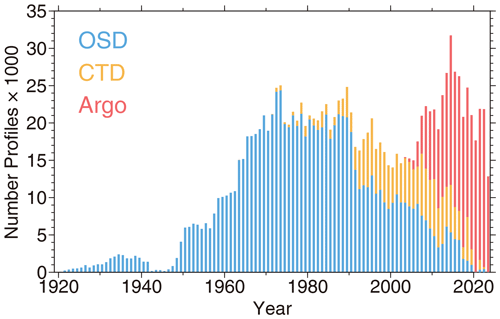
Figure 1 Yearly number of oxygen profiles from the World Ocean Database (OSD and CTD profiles) and national DACs (Argo) from 1920 to 2023.

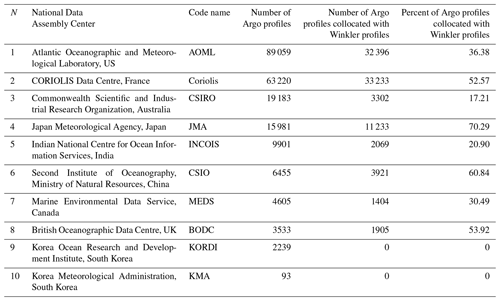
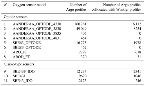
Numbers of oxygen profiles disseminated by 10 national Argo DACs and used for the current study are given in Table 1. The most considerable contribution comes from two DACs: the Atlantic Oceanographic and Meteorological Laboratory (AOML) and the French CORIOLIS Data Centre (Coriolis). Together, these two DACs contribute 71 % of all oxygen profiles. The global sampling by Argo floats is characterized by big gaps in the tropical belt of the World Ocean (Fig. 2c) and in the marginal seas with shallow bottom depths.

The DACs report oxygen data along with quality flags set after the QC procedure performed by each DAC. The spatial distribution of the profiles from each DAC is shown in Fig. 3. Only the AOML dataset is characterized by a more or less global coverage. The profiles from the second large Coriolis dataset are concentrated mostly in the Atlantic and Southern oceans. Other DACs are characterized by a regional scope: Japan Meteorological Agency (JMA) data come from the Pacific Ocean east of Japan, profiles from the Commonwealth Scientific and Industrial Research Organization (CSIRO) cover the Southern Ocean, China Second Institute of Oceanography (CSIO) mainly provides Argo profiles from the subtropical and tropical western Pacific Ocean and Argo profiles from the British Oceanographic Data Centre (BODC) are located in the Atlantic Ocean. Profiles from the Korea Ocean Research and Development Institute (KORDI) and from the Korea Meteorological Administration (KMA), the smallest two datasets, are located in the southern part of the Sea of Japan.

3 Data quality control

Quality evaluation of hydrographic data typically consists of two parts: data QC for random errors and evaluation of systematic errors or biases. These two issues are often treated separately but represent the entire QC procedure. A unified QC procedure has yet to be suggested for the global archive of oxygen profile data, and oxygen-related studies often rely on WOD (Garcia et al., 2019), Argo (Thierry et al., 2021), and Bushnell et al. (2015) QC procedures. The efforts undertaken under the International Quality-Controlled Ocean Database (IQuOD) initiative (Cowley, 2021) resulted in a comprehensive study, where different quality control procedures for temperature profiles were compared and evaluated (Good et al., 2022). As shown in the previous section, the characteristic feature of the global oxygen data archive is its heterogeneity. In the early years, a relatively small amount of data permitted expert quality control, but for the actual global archive, automated quality control (AutoQC) procedures are required.

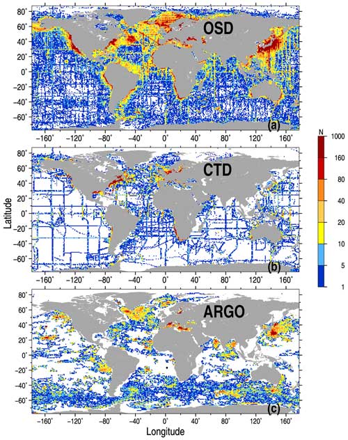
Figure 2 Number of profiles (N) in 1°×1° latitude–longitude squares for OSD (a), CTD (b), and Argo (c) data.

The AutoQC procedure aims to identify and flag outliers, which represent observations significantly deviating from the majority of other data in the population. Monhor and Takemoto (2005) noted that there is no rigid mathematical definition of an outlier. The outliers do not necessarily represent erroneous measurements and can occur due to the natural variability of the measured variable. A QC procedure defines outliers using a set of thresholds, which are based on physical laws (for instance, the maximum solubility of gases in the water) or have to be defined based on the statistical properties of the data population.

In this paper, we introduce a novel QC procedure capable of conducting quality assessment of data from different instrumentation types. The procedure is applied to the observed level data and does not require additional quality checks for profiles interpolated at a predefined set of levels. This second level of QC is an attribute of the WOD QC system (Garcia et al., 2019). To increase the reliability in detecting erroneous data, a set of quality checks is applied to each profile. The larger the number of failed distinct quality checks, the higher the probability that the flagged observation represents a data outlier. Based on the available QC schemes for oceanographic data (most of them were developed for temperature and/or salinity profiles), quality checks can be subdivided into the following groups:

• Group 1 – check of location, date and bottom depth of the profile;

• Group 2 – check of profile attributes (maximum sampled depth, number of levels, variables measured) specific to each instrumentation type;

• Group 3 – range check, e.g., comparison of observations at each level against minimum/maximum value thresholds, which are set for the entire ocean or oceanic basin (global ranges) or for the particular location and depth;

• Group 4 – check of the profile shape, which is characterized by the vertical gradient of the measured variable at observed levels, by the number of local extrema, and by the presence of spikes.

It should be noted that QC procedures often assume Gaussian distribution law, and outliers are defined in terms of multiple times the standard deviation from the mean value (Z-score method). For instance, the WOD standard deviation check is based on this assumption (Garcia et al., 2019; Boyer et al., 2018). However, distributions of oceanographic parameters are typically skewed, and the assumption of Gaussian distribution leads to false data rejection. Tukey (1977) introduced a so-called box-plot method, which makes no assumption about the distribution law and is often used for outlier detection. Hubert and Vandervieren (2008) developed the adjusted Tukey's box-plot method for skewed distribution with fences depending on skewness. Following this approach, Gouretski (2018) and Tan et al. (2023) applied QC checks, taking into account the skewness of temperature distribution. In the current study we use the Hubert and Vandervieren (2008) adjusted box-plot method as modified by Adil and Irshad (2015).

Table 1 Argo oxygen profiles from different national DACs.

Developing the QC procedure, consisting of a suite of distinct checks, we assume that oxygen data obtained by the reference Winkler method are superior in quality compared to the sensor data. As noted by Golterman (1983), the principle of the Winkler method has been unchanged since its introduction, with the method still providing the most precise determination of dissolved oxygen. There is a total of 10 distinct quality checks, which are introduced in Sect. 3.1 to 3.9. The outlier statistics are shown in the Supplement (Figs. S1–S10), both for the year–depth bins and within 2°×4° geographical boxes and for randomly selected oxygen profiles affected by the respective check.

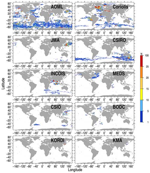
Figure 3 The number (N) of Argo oxygen profiles in 1°×1° spatial boxes for the datasets from different DACs. The name abbreviation of each DAC is also presented in each panel.

3.1 Geographical location check

A comparison of the deepest sampled level with the local ocean bottom depth may be used for the identification of erroneous geographical locations. We use a GEBCO 0.5 min resolution digital bathymetry map to define thresholds for this check. For each profile, the range between minimum and maximum GEBCO bottom depth within the 111 km radius is calculated. If the difference between the deepest profile measurement depth and the local GEBCO depth exceeds the above-depth range, the geographical coordinates of the profile are considered to be in error, and data at all levels are flagged. According to Table 2, about 0.5 % of OSD and CTD profiles fail this check, compared to only 0.08 % for Argo profiles. For each data type, the spatial distribution of profiles failing this test exhibits a rather random pattern (Fig. S1). The highest percentage of OSD outlier profiles is found for the time period before 1946, probably due to less accurate navigation methods during the war (Fig. S1b). CTD profiles exhibit higher outlier scores above 400 m between 200–2014, linked to several cruises. Only 0.077 % of DAC QC-ed Argo profiles fail this check (Fig. S1g–i).

3.2 Global oxygen range check

The test is applied to identify observations that are grossly in error (so-called “blunders”). These data correspond to the cases of the total instrumentation fault or crude errors introduced during the data recording or formatting. The overall minimum–maximum oxygen ranges are defined based on the entire archive of the OSD profiles. These overall ranges are set for depth levels and temperature surfaces because the maximum oxygen solubility depends on temperature. For the construction of overall limits, we use the normalized frequency histograms (Fig. 4). The depth–oxygen histograms are constructed similarly with normalization at each depth level (Fig. 4b). The normalization is done to account for varying numbers of oxygen observations with depth and temperature. The relative frequencies serve as guidance to produce the overall oxygen minimum and maximum limits, which approximately correspond to the relative frequency of 0.05 (indicated by the green lines). The spatial distribution of the OSD and CTD profiles with levels failing this check broadly corresponds to the sampling density (Figs. S2a and d, S3a and d), whereas flagged Argo profiles can be rather linked to distinct floats (Figs. S2g, S3d). The CTD data are characterized by the largest fraction of profiles affected by this check (Figs. S2e, S3e).

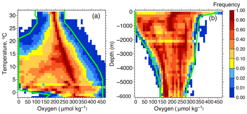
Figure 4 Normalized oxygen histograms used to define overall oxygen ranges versus temperature (a) and versus depth (b). Minimum and maximum overall oxygen limits are shown by solid green lines. For each temperature–oxygen bin in (a), the number of oxygen observations is divided by the number of observations in the most populated bin for the same temperature. The depth–oxygen histograms (b) are constructed similarly with normalization at each depth level.

3.3 Maximum oxygen solubility check

According to Henry's law, the quantity of an ideal gas that dissolves in a definite volume of liquid is directly proportional to the partial pressure of the gas. It is also known that gas solubility in the water typically decreases with increasing temperature. The histograms of observed oxygen concentration (C_obs) versus maximum oxygen solubility (C_max) calculated using reported temperature and salinity in different ocean layers depict a close relationship between the mode of observed oxygen distribution and the maximum solubility (Fig. 5a–d). The histograms also show that the distribution mode for the upper-most layer 0–100 m (Fig. 5a) follows the line $C_{\mathrm{obs}}=C_{max}$, progressively deviating to lower C_max values when C_obs>300 µmol kg⁻¹, suggesting an oxygen supersaturation. That is because in the photic layer of the ocean oxygen is produced by phytoplankton through photosynthesis, and oxygen supersaturation can evolve. Oxygen production due to photosynthesis leads to the formation of small bubbles (10–70 µm) with increasing oxygen supersaturation accompanied by a higher number of bubbles and their shift towards large sizes (Marks, 2008). In the deeper layers (Fig. 5b–d), the number of cases with supersaturation decreases because of the reduced photosynthesis, so the temperature and pressure effects dominate. According to the histograms (Fig. 5a–d), supersaturation is frequently observed in the upper layers. The percentage of supersaturated values decreases from about 45 % in the near-surface layer to less than 1.0 % below the 200 m level (Fig. 5e, red).

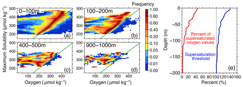
Figure 5 Supersaturation check: (a–d) normalized frequency histograms for maximum solubility versus reported dissolved oxygen values for different layers. The bin size is 10 µmol kg⁻¹. For each maximum solubility level, the frequencies for each bin are normalized by the number of the values in the most populated bin in order to account for variations in the number of profiles. (e) Percentage of supersaturated oxygen values over all observed oxygen values (red) and the threshold for the supersaturation check, represented by the percentage relative to the maximum solubility (blue).

In order to set the threshold percentage for supersaturation, we calculated histograms of supersaturation values for each 1 m depth level of the upper 500 m layer. The threshold percentage of supersaturation (Fig. 5e, blue line) corresponds to the 99th quantile. The threshold value approaches 100 % near the depth of 200 m; therefore, below 200 m all supersaturated oxygen values are flagged. Locations of profiles with at least one observed level failing this check are shown in Fig. S4a, d, and g. The distribution of profiles broadly corresponds to the spatial sampling density. The OSD outliers are more numerous in the early years before 1955, probably pointing to less accurate measurements during that time period. The check reveals a much higher percentage of CTD outliers throughout the water column for several years before 2000 (Fig. S4b) compared to other instrumentation types. Argo floats are characterized by the low outlier percentage for this quality check, with a higher percentage found for deep Argo floats between 2017–2018 below 2000 m (Fig. S4h).

3.4 Stuck value check

Malfunctioning of sensors often results in stuck values when the same oxygen concentration is reported for all or most of the observed levels. To identify such profiles, we calculated oxygen standard deviations for each oxygen profile to build histograms (Fig. 6) for each instrumentation type. Only profiles with at least seven oxygen levels are considered. Unlike the OSD and Argo data, for which the frequency of profiles drops for low standard deviation values, the CTD profiles are characterized by a distinct peak for the lowest standard deviation values (Fig. 6c). Accordingly, based on the histograms (Fig. 6b, c), we set the thresholds of 3 and 1 µmol kg⁻¹ and for CTD and Argo profiles, respectively. No lowest value thresholds are applied for OSD profiles, as stuck values are only characteristics of the electronic sensors. The geographical distribution of profiles failing this check is given in Fig. S5a and d. The check is applied only to the CTD and Argo sensor data and reveals a high percentage of outliers for CTD profiles, especially after 2000 (Fig. S5b). Argo profiles which fail the check are not numerous and are mostly located in the Northern Hemisphere (Fig. S5d).

Figure 6 Oxygen profile standard deviation for OSD (a), Argo (b), and CTD (c) instrumentation types. Only profiles with at least seven levels of oxygen data are considered. Red vertical lines show the respective threshold values for Argo and CTD profiles.

3.5 Multiple extrema check

The multiple extrema check aims to identify profiles whose shape significantly deviates from the majority of profiles. For each profile with at least seven observed levels (black dots), the number of local extrema and their magnitudes (denoted as M_n in Fig. 7a, defined as oxygen difference between two adjacent oxygen measurements) are calculated. Then, the normalized frequency histograms of oxygen profiles for different combinations of the number of oxygen extrema and of the extremum magnitude are calculated for three instrumentation types separately (Fig. 7b–d). The larger the extremum magnitude, the less frequent the corresponding profiles. Physically, an oxygen profile at a location is not likely to exhibit both too large and too frequent oscillations of oxygen concentrations. Thus, the profiles with many or big extrema are likely erroneous. The histogram for Argo profiles differs from that for OSD and CTD because it is based on profiles already validated by the respective DACs. The multiple extrema check thresholds (black lines in Fig. 7b–d) are defined using the histograms as guidance. The lines crudely correspond to the normalized frequency of 0.01 for OSD and CTD and 0.05 for Argo profiles. The geographical distribution of profiles failing the check is given in Fig. S6a, d, and g. Argo profiles failing the check can be linked to distinct floats (Fig. S6g). The OSD profiles exhibit a higher outlier percentage for the years 1990–2002. The highest rejection rate for the CTD profiles is typical of the years before 2000 (Fig. S6b, e).

Figure 7 (a) Schematics for the multiple extrema check. Black dots represent the observed values, and local extrema are defined by M, whereas extremum magnitudes are shown with blue lines. (b–d) Normalized frequency histograms for multiple extrema checks for OSD (b), CTD (c), and Argo (d). The area to the right of the black line corresponds to oxygen profiles failing the multiple extrema check.

3.6 Spike check

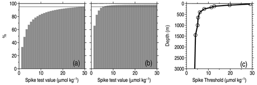
Spikes are the values at levels that strongly deviate from the values at the nearest levels above and below. For each observed level k, the test value $s=s_{\mathrm{1}}-s_{\mathrm{2}}$ is calculated, where $s_{\mathrm{1}}=|p_k-\mathrm{0.5}(p_{k-\mathrm{1}}-p_{k+\mathrm{1}}\left)\right|$, $s_{\mathrm{2}}=\left|\mathrm{0.5}\right(p_{k+\mathrm{1}}-p_{k-\mathrm{1}}\left)\right|$, and p denotes the oxygen value. The observation is identified as an outlier when the test value s exceeds a threshold value. Due to the larger oxygen variability in the upper layers, we set depth-dependent spike thresholds, which are defined for nine depth layers using accumulated histograms for the test value s (Fig. 8a and b for 0–100 and 400–600 m as examples). The threshold profile is defined by the 95 % frequency at each layer (Fig. 8c). The 95 % value is chosen empirically but can be tuned when additional QC-ed benchmark datasets become available. Examples of profiles which failed this check are shown in Fig. 7s. Data from all instrument types are characterized by a rather homogeneous temporal and spatial distribution of outliers.

Figure 8 Spike check value histograms (see text for details) for the layer 0–100 m (a) and 400–600 m (b) and spike check value threshold versus depth (c).

3.7 Local climatological oxygen range check

The local climatological oxygen range check is one of the most effective QC modules for identifying outliers compared to other checks because the minimum–maximum thresholds are constrained by the local water mass characteristics. For each 1°×1° latitude–longitude grid point, we calculate min–max thresholds, accounting for the skewness of the data. For calculating climatological ranges, we take the ergodic hypothesis in which the average over time is considered to be equal to the average over the data ensemble within a certain spatial influence radius. Taking into account the skewness of statistical distribution when defining climatological ranges for oceanographic parameters was first suggested by Gouretski (2018), who applied Tukey's box-plot method, modified for the case of skewed distributions (Hubert and Vandervieren, 2008; Adil and Irshad, 2015). In this method, lower (Lf) and upper (Lu) fences are calculated according to formula (1):

$$\begin{array}{}\text{(1)}& \begin{array}{rl}\left[\text{Lf Uf}\right]& =[Q\mathrm{1}-\mathrm{1.5}\cdot \text{IQR}\cdot \exp (-\mathrm{SK}\cdot \left|\text{MC}\right|)Q\mathrm{3}\\ & +\mathrm{1.5}\cdot \text{IQR}\cdot \exp (\mathrm{SK}\cdot |\mathrm{MC}\left|\right)],\end{array}\end{array}$$

where Q1 and Q3 are quartiles, Q2 is the sample median, and SK is skewness. MC denotes the medcouple, which is defined as MC = median h(x_i,x_j), where $x_i\le Q\mathrm{2}\le x_j$, and the kernel function $h(x_i,x_j)=\left[\right(x_j-Q\mathrm{2})-(Q\mathrm{2}-x_i\left)\right]/(x_j-x_i)$ (Hubert and Vandervieren, 2008).

The local oxygen ranges are constructed using both the OSD and Argo oxygen profiles. The OSD used to derive the local threshold have undergone the preliminary QC (checks for global oxygen range, spikes, stuck values, multiple extrema), aiming to remove crude outliers to reduce their impact on the local thresholds. This approach is similar to the two-stage thresholding suggested by Yang et al. (2019). The Argo oxygen profiles underwent quality control at the respective DACs.

The local minimum and maximum thresholds were calculated at 1°×1° grids at a set of 65 depth levels corresponding to the levels implemented for the World Ocean Circulation Experiment – Argo Global Hydrographic Climatology (Gouretski, 2018) using Eq. (1). Examples of the threshold spatial distribution are presented for two depth levels: 98 m (level typically located below the seasonal thermocline, Fig. 9a–c) and 1050 m (level typically located below the main thermocline, Fig. 9d–f). The most striking features are the areas with low minimum oxygen values (oxygen minimum zones, Fig. 9a, b) in the east Pacific, Arabian Sea, Bay of Bengal, Black Sea, and Baltic Sea. The oxygen range map for level 98 m (Fig. 9c) shows that the areas with the widest local ranges coincide with minimum oxygen zones. The local range map for the 98 m level also depicts wider ranges in several highly dynamic regions of the Gulf Stream, Malvinas current, and the area north of the Antarctic coast (Fig. 9c). During the QC, gridded minimum and maximum local oxygen values are interpolated to the observed levels at profile locations. The geographical distribution of profiles failing the check is given in Fig. S8a, d, and g, indicating a rather uniform temporal and spatial distribution. A decrease with time of the outlier percentage for OSD is clearly seen. For CTD data, the outlier percentage is high for all levels and years except for the years after 2020. Argo profiles failing the check in many cases can be linked to the data from particular floats (Fig. S8g).

3.8 Local climatological oxygen gradient range check

The oxygen vertical gradient check aims to identify pairs of levels for which the vertical oxygen gradient exceeds a certain threshold. Threshold values for the vertical gradient (Fig. 9g–l) are calculated using Eq. (1), similar to the local oxygen ranges. Due to the nonlinearity of oxygen profiles, vertical gradient values depend on the profile's vertical resolution, e.g., from the gap between two neighbors' observed levels. Respectively, oxygen thresholds have been calculated for several depth gaps between 10 and 100 m, as Tan et al. (2023) did for the QC of temperature profiles.

For level 98 m, the spatial distribution of the oxygen gradient range (Fig. 9i) is similar to the spatial pattern of the oxygen range (Fig. 9c), with the largest ranges located in the oxygen minimum zones, reflecting the highest oxygen variability in these areas. The region below the main thermocline (Fig. 9j–l) is characterized by a much smaller range compared to the 98 m level (Fig. 9g–i). The geographical distribution of profiles failing the check is given in Fig. S9a, d, and g, indicating a rather uniform temporal and spatial distribution broadly corresponding to the sampling density. For CTD data, the lowest outlier percentage is observed after 2000 (Fig. S9e).

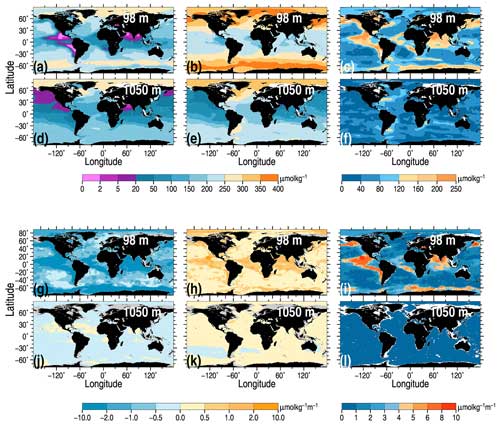
Figure 9 Upper six panels: maps of the lower (a) and the upper (b) climatological oxygen threshold and of the oxygen range (c) for the 98 m depth level. (d–f) Same but for the 1050 m depth level. Lower six panels: maps of the lower (g) and the upper (h) climatological oxygen vertical gradient threshold and of the oxygen vertical gradient range (i) for the 98 m depth level. (j–l) Same but for the 1050 m depth level.

3.9 Excessive flagged level percentage check

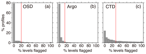
After applying all previous quality checks, the percentage of flagged levels for each oxygen profile is calculated to produce histograms in Fig. 10. A threshold is set based on these histograms to decide on the quality of the entire profile: we set 20 %, 15 %, and 30 % thresholds for OSD, Argo, and CTD profiles, respectively. If the threshold is exceeded, the entire profile is flagged, and it is suggested that it not be used in future analyses. Both the OSD and Argo datasets are characterized by a low number of profiles with a high percentage of flagged data. In contrast, for the CTD group, the histogram (Fig. 10c) exhibits a thick and long tail, with a significant fraction of profiles having a high percentage of flagged levels.

The geographical distribution of profiles failing the check is given in Fig. S10a, d, and g, indicating a rather uniform temporal and spatial pattern. A decrease in the outlier percentage with time for OSD is seen after about 2005 (Fig. S10b). For CTD data, the outlier percentage is high for all years except 2021. Argo profiles failing the check in many cases can be linked to distinct floats (Fig. S10g).

Figure 10 Percentage of oxygen profiles versus percentage of rejected levels per profile for OSD (a), Argo (b), and CTD (c) instrument types.

4 Evaluation of the QC procedure

Table 2 and Fig. 11 summarize the rejection rates for all 10 quality checks for the three instrumentation types separately. The Argo oxygen profiles have the lowest overall rejection rate of 4.8 %, with Winkler data quality ranking second best (12.0 % outliers). The difference might likely originate from (1) Winkler profiles covering a century-long period of observations, with a poor data quality in the earlier decades, and (2) the analyzed Argo oxygen data being represented by adjusted profiles, which have been already quality-controlled.

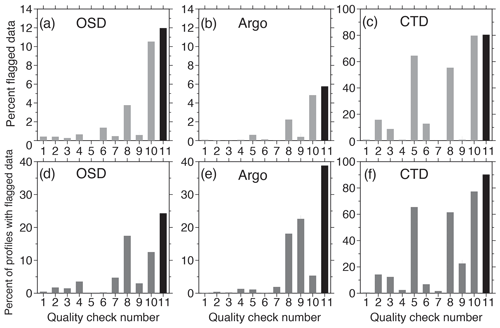
Figure 11 (a–c) Percent of measurements flagged by distinct quality checks for three instrumentation types and (d–f) percent of profiles with at least one measurement flagged. For the description of checks, see Table 2. The black bar at the number 11 corresponds to the total percent of flagged data (a–c) and to the percent of profiles flagged by at least one quality check (d–f).

The CTD oxygen profiles have the highest percentage of outliers (overall rejection rate of 80.0 %). The significant part of CTD oxygen outliers is attributed to the stuck value check, which searches for profiles with identical or very similar oxygen values at all observed (reported) levels (Fig. 11a, check 5). Most of these profiles also fail the local climatological range check. We note that these profiles have also been identified as outliers during the compilation of the WOA18 (Garcia et al., 2019) and WOA23 (Garcia et al., 2024) atlases of dissolved oxygen and have not impacted climatological oxygen distributions presented in these atlases.

As introduced above, the local climatological range check (check 8 in Table 2) represents the most important quality check and results in the highest percentage of flagged observations and profiles. For OSD, about 17.5 % of profiles have at least one measurement flagged by this check. For Argo and CTD profiles, these values are 18.1 % and 61.5 %, respectively.

Figure 12 shows the percentage of flagged measurement versus time and depth and within 1° latitude–longitude boxes for three main instrumentation types. The OSD group exhibits a graduate decrease in outlier percentages with time at all depths (Fig. 12a), indicating the gradual improvement of data quality with time, especially after the early 1990s, which coincides with the beginning of the extensive observational activities during the World Ocean Circulation Experiment (WOCE). The global spatial pattern of outliers (Fig. 12b) is characterized by outlier percentages lower than 5 % in most 1° grid cells, with only a few areas exhibiting higher percentages, which can be linked to some particular cruises or observational programs.

Oxygen data from Argo floats (Fig. 12c, d) are characterized by a low percentage of outliers reflecting the impact of the QC and data adjustments already conducted at DACs. We also find no clear time trend in outlier scores. There is an indication of higher outlier percentages in the layer below 1500 m before 2020 (Fig. 12c). Strong spatial contrasts in the percentage of Argo outliers (Fig. 12d) in most cases can be linked to particular Argo floats.

Unlike the OSD Winkler data, CTD oxygen profiles do not suggest a time trend in data quality (Fig. 12e). Compared to both OSD and Argo, ship-based CTD oxygen profiles are characterized by a much higher outlier percentage. This is explained through a significant fraction of CTD profiles failing the stuck value check, local climatological range check, and excessive flagged level percentage check (Table 2). The CTD outlier profiles are evenly distributed over the oceans (Fig. 12f). Figure 12g and h show outlier distributions for the profiles that passed both the stuck value and the multiple extrema checks. In this case, most cruise lines (Fig. 12h) are characterized by a low outlier percentage, with data quality issues related to a smaller subset of cruises. Finally, we find that the CTD data since 2018 (Fig. 12g) exhibit very low outlier scores comparable to those of OSD and Argo float profiles.

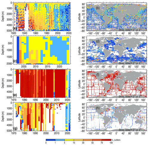
Figure 12 Percentage of flagged observations in year–depth bins (a) and in 1° latitude–longitude boxes (b) for OSD oxygen profiles. (c, d) Same but for Argo oxygen profiles, (e, f) same but for CTD oxygen profiles, and (g, h) same but for CTD oxygen profiles that passed multiple extrema and stuck value quality checks.

Table 2 Outlier score statistics for different instrumentation types.

5 Benchmarking of the QC procedure using manually controlled datasets

Evaluation of the QC system is a crucial part of the dataset generation. Good et al. (2022) conducted a comprehensive benchmarking exercise to evaluate the performance of automated QC checks for temperature profiles implemented by different research groups, aiming to recommend an optimal set of quality checks. They used several reference datasets with known quality (e.g., bench-marking datasets whose quality was manually evaluated by experts).

Unfortunately, in a deviation from temperature profiles, no community-agreed oxygen datasets exist which could be used for benchmarking. In this study, we use for the bench-marking a comprehensive set of bottle profile data obtained during the World Ocean Circulation Experiment (WOCE) – the largest international oceanographic experiment ever conducted (Wunsch, 2006). To achieve high data quality and consistency between the cruises over the entire period of observations, the WOCE Hydrographic Program Office (WHPO) issued operation manuals (WHPO, 1991), where measurement methods and procedures are described. As shown by Gouretski and Jancke (2000), the WHPO quality requirements have been fulfilled, with the WOCE hydrographic dataset representing a unique global scale high-quality collection of the whole suite of oceanographic parameters. Specifically, the mean inter-cruise oxygen offset was found to be 2.39 µmol kg⁻¹. Upon completing the WOCE, the GO-SHIP program was established in 2007 to revise the WOCE hydrographic program by repeating several WOCE lines (Hood et al., 2010).

Applying our QC procedure to the entire WOCE dataset confirms the high quality of this unique dataset, with only 2.8 % of oxygen outliers (Fig. 13a, b) from the total of 354 028 oxygen measurements for the entire time period 1990–1998. Similar to the entire OSD dataset, the QC diagnostics reflect the progressive improvement of the oxygen data quality over the period of WOCE (Fig. 13a). The spatial distribution of outliers for the entire time period (Fig. 13c) indicates that the majority of WOCE oxygen profiles have a very low percentage of outliers. For 79 % of WOCE oxygen profiles, our QC procedure identified no data outliers. The higher rejection rate is found only for several WOCE lines in the tropical South Atlantic, northwestern Indian Ocean, and the Labrador Sea. We note that, in the same areas, there are data from other cruises which exhibit low outlier percentages, so the flagging cannot be attributed to the spatial selectivity of the QC procedure.

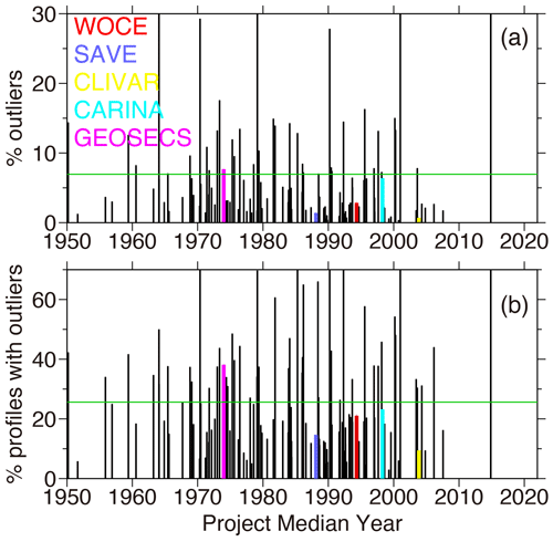
The WOD permits data selection for a large number of observational programs using the respective project identification code. The outlier rejection percentage for the data from 128 projects that reported oxygen data is shown in Fig. 14. The mean rejection rate over all projects is 7 %. Apart from WOCE, several outstanding observational programs like GEOSECS (Geochemical Ocean Sections Study) (Craig, 1974), SAVE (South Atlantic Ventilation Experiment) (Larqué et al., 1997), CARINA (Carbon dioxide in the Atlantic Ocean) (Falck and Olsen, 2010), and CLIVAR (Climate and Ocean: Variability, Predictability and Change) (Sarachik, 1995) delivered a significant number of high-quality hydrographic data with quality documented in the literature. We note that the four projects with a median year after 1985 (SAVE, WOCE, CARINA, and CLIVAR) are characterized by rejection rates lower than the mean. The 8 % outlier rate for one of the largest international GEOSECS experiments conducted in the 1970s only slightly exceeds the mean outlier percentage over all 128 projects.

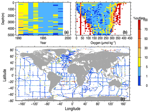
Figure 13 QC statistics for the WOCE dataset: (a) percentage of outliers in year–depth bins, (b) percentage of outliers in oxygen–depth bins, and (c) percentage of outliers in 1°×1° squares.

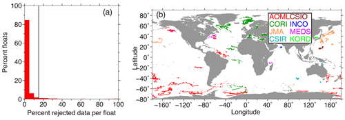
Finally, we used the delayed-mode quality-controlled Argo data to evaluate the performance of our QC procedure. The Argo dataset used for the current study consists of oxygen profiles reported from 1794 floats. The histogram of the percentage of flagged observations for each Argo float (Fig. 15a) shows that for 90 % of all floats, the percentage of rejected observations is less than 15 %, with 84 % of floats exhibiting less than 5 % of rejected measurements. We conclude that the QC applied in the DACs effectively identifies data outliers for the majority of the floats, resulting in a low outlier percentage (see Fig. 12c, d). The location map of profiles from Argo floats with more than 15 % of data flagged over the float lifetime (Fig. 15b) shows a rather random distribution throughout the world ocean, with almost all DACs contributing with such floats. We interpreted this result as an implicit confirmation of the ability of our QC scheme to identify data with quality issues.

Figure 14 Outlier diagnostics for 128 distinct WOD projects (OSD Winkler profiles): (a) overall percent of outliers and (b) percent of profiles with oxygen outliers. Acronyms and percentages for selected hydrographic projects described in text are shown in color.

Figure 15 (a) Percent of Argo oxygen profiles versus percent of flagged data per profile and (b) trajectories of Argo floats with more than 15 % of flagged data (a total of 127 floats).

6 Bias assessment for sensor oxygen data

The QC procedure described in the previous sections is based on the underlying statistics of the data and aims to identify random outliers. The second step in data QC is estimating the possible systematic errors or biases. These systematic errors may differ depending on the instrumentation type, but the common cause for systematic errors is the absence of the possibility to calibrate the instrument. A classic example provides temperature data obtained by eXpandable BathyThermographs (XBTs) where systematic errors are due to the uncertainty in depth, which is calculated from the elapsed time, and the uncertainty in thermistor, which is typically not calibrated (Gouretski and Reseghetti, 2010; Cheng et al., 2014).

In the case of dissolved oxygen, only Winkler oxygen determinations of discrete samples can be considered to be bias-free because the chemical analysis is based on the standard reference, with the replicate measurements having a precision better than 0.4 µmol kg⁻¹ (Taillandier et al., 2018). However, differences in methods and standards between hydrographic cruises suggest a lower level of data precision. Gouretski and Jancke (2000) used the high-quality WOCE one-time hydrographic dataset and conducted a comprehensive analysis of the inter-cruise oxygen differences at the cruise cross-over areas. The analysis was performed in the deep part of the water column (typically below 2000 m), where the time variations of seawater properties are small. For 305 cross-over areas, they estimated the mean difference between WOCE cruises to be 2.40 µmol kg⁻¹ with a standard deviation of 2.37 µmol kg⁻¹. Considering stringent criteria for the WOCE hydrographic program, this estimate can be considered to represent an approximate precision of the Winkler method in application to real hydrographic data. As noted by Golterman (1983), the Winkler method still represents the most precise determination of dissolved oxygen. In spite of some modifications over time, the principle of the method is unchanged. In the following, we describe residual biases for CTD and Argo profiles. The term “residual” is used because CTD oxygen profiles are often adjusted on Winkler bottle samples, and Argo oxygen profiles used in our study undergo adjustment procedures at the respective DACs.

The use of electrochemical and optical oxygen sensors in oceanographic practice has two main aspects. First, these sensors permitted a significantly higher rate of data acquisition and a much finer vertical resolution than bottle data. Secondly, they made the observational process much easier than bottle samples, which need chemical titration in the laboratory. However, like other electronic sensors, oxygen sensors are prone to offsets and drift. Takeshita et al. (2013) analyzed data from 130 Argo floats and found a mean bias of −5.0 % O₂ saturation at 100 % O₂ saturation. Bittig et al. (2018) explained this negative bias by the reduction of O₂ sensitivity proportional to oxygen content, with the decrease in sensitivity being on the order of several percent per year. Optode drift characteristics require regular calibration. Use of reference Winkler profiles is only possible for the ship-based CTD oxygen sensors (mostly electrochemical sensors) if CTD rosette water samples are obtained simultaneously with sensor profiles and are analyzed for oxygen during a cruise (Uchida et al., 2010). For uncrewed autonomous platforms like Argo, the direct comparison with reference Winkler data is limited to samples from the hydrographic casts conducted during the float deployment. Bittig et al. (2018) recommended adjusting optode data on oxygen partial pressure primarily by the gain (the Argo Quality Control Manual; Thierry et al., 2021). If no previous delayed-mode adjustment is available, the basic real-time adjustments are performed based on the oxygen saturation maps provided by the WOA digital climatological atlas (Thierry et al., 2021). In the case that a delayed-mode adjustment is not available after 1 year, the re-assessment of the gain factor is recommended. Uncertainty in underlying optode calibration and time drift characteristics leads to errors in adjusted data.

6.1 Bias assessment method

We aim to assess the magnitude of the possible overall residual bias for CTD profiles and adjusted Argo profiles by comparing these profiles with collocated reference discrete samples. The data from 10 national DACs were used for this analysis, for which both unadjusted and adjusted oxygen profiles are available. Data centers and the respective number of oxygen profiles are given in Table 1. Data using the Winkler method are used as reference data for the comparison with collocated Argo oxygen profiles.

For the current analysis, we selected a 100 km threshold distance within which two profiles are spatially collocated. To decide upon the choice of the optimal maximum time difference between Argo and reference profiles, we calculated median oxygen offsets the increasing threshold value for the time separation between a pair of profiles (Fig. 16a). Increasing the temporal collocation bubble leads to the increase in the bias magnitude in agreement with the assumption that the older reference data are richer in oxygen compared to the more recent data. Below 1000 m depth, the difference between the median offsets for the temporal collocation bubble of 5 and 50 years is about 3.5 µmol kg⁻¹, corresponding to a deoxygenation trend of about 0.7 µmol kg⁻¹ per decade. This estimate can be compared with 0.75 µmol kg⁻¹ per decade reported by Grégoire et al. (2021). As Fig. 16c suggests, the overall offset estimate below 1000 m stabilizes after the time difference threshold of 5 years. The extension of the temporal bubble for more than 7 years leads to the progressive increase in the bias magnitude, which we attribute to the impact of the general deoxygenation. Based on these calculations, the 5-year threshold was selected as the maximum time separation between collocated profiles. For this threshold value, the number of collocated pairs below 1000 m depth is about 10 000 (Fig. 16b). A step-wise decrease in the number of collocated pairs below 950 m is explained by a significant part of reference profiles being limited to the upper 1000 m layer. These calculations suggest that about 1000 collocated pairs are required for stable offset estimates.

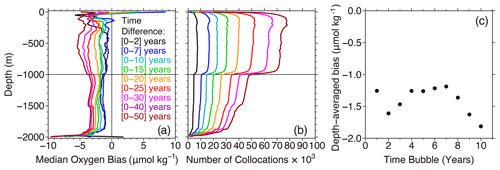
Figure 16 (a) Overall median oxygen bias versus the size of the temporal collocation bubble, (b) number of collocated pairs for different choices of collocation bubbles, and (c) depth-averaged (1000–1900 m) bias versus time bubble size.

The number of Argo profiles having collocations with discrete ship-based Winkler profiles is shown in Table 1. No collocated Winkler profiles are found for the Argo profiles from the two South Korean DACs. Profiles from these DACs are restricted within a relatively small area east of the Korean Peninsula. The four largest contributors of Argo data (AOML, Coriolis, JMA, and CSIRO) comprise up to 90 % of all Argo profiles having collocations with reference profiles.

6.2 Overall bias characteristics of unadjusted and adjusted Argo oxygen data from DACs

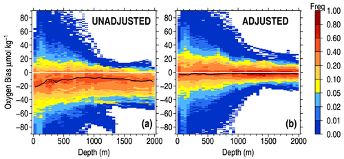
The normalized frequency histograms (Fig. 17) characterize the spread of individual bias estimates around the distribution mode. These histograms are based on all Argo profiles having collocations with reference Winkler data. In these histograms, for each depth bin, the number of values in each bias bin is normalized by the number for the most populated bias bin at each depth level to account for the decrease in data with depth. The histograms are shown for raw (unadjusted) (Fig. 17a) and adjusted Argo profiles (Fig. 17b). The adjustment procedures applied at different DACs reduce the spread of the individual bias estimates and the skewness of the bias distribution, with the overall median bias of 10–12 µmol kg⁻¹ for unadjusted data and 1–2 µmol kg⁻¹ for adjusted data. As suggested by the bias distribution with depth, we estimate residual bias using the collocated data below 1000 m depth, where the bias spread reduces significantly compared to the upper part of the water column.

Figure 17 Normalized histograms of the unadjusted (a) and adjusted (b) Argo oxygen bias versus collocated Winkler profiles. The black lines show the median bias value.

6.3 Residual oxygen biases for distinct oxygen sensor

A total of 11 oxygen sensor models were implemented on BGC Argo floats, with 8 sensor models found among Argo profiles having collocations with reference data (see Table 3). Figure 18 shows the yearly number of Argo profiles that have collocations with reference data and are equipped with different models of oxygen sensors. The SBE43-series sensors are electrochemical Clark-type sensors, whereas all other models are optical sensors (optodes). Since the beginning of the 2000s, several models of optodes have been implemented in BGC Argo floats. The two most widespread sensors are AANDERAA 3830, implemented between 2004 and 2018, and the newer model AANDERAA 4330 used since 2010. The majority of Argo floats from the three largest AOML, Coriolis, and JMA datasets have been equipped with this sensor. Data from AOML, Coriolis, JMA, and CSIRO include oxygen profiles obtained by means of several sensor models. The other four DAC subsets of data are represented by a single sensor model: AANDERAA_OPTODE_4330 prevails in the data from INCOIS, CSIO, and BODC, and AANDERAA_OPTODE_3830 is typical of MEDS data. AROD_FT and ARO_FT optodes have only been implemented on Argo floats managed by JMA.

Table 3 Oxygen sensors installed on BGC Argo floats.

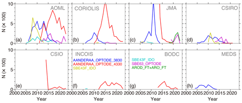
Figure 18 Yearly number of BGC Argo profiles equipped with different types of oxygen sensors (colored lines; see sensor attribution in panel (e)). (a) AOML, (b) Coriolis, (c) JMA, and (d) CSIRO and (e) CSIO, (f) INCOIS, (g) BODC, and (h) MEDS.

According to the Argo Quality Control Manual (Thierry et al., 2021), several adjustment procedures can be applied to unadjusted data (adjustment to climatology, nearby Winkler samples, or in-air data). The adjustment results may depend on many factors, such as the subjective decision of the operator in a DAC, the use of specific software, and the availability of the respective reference data. If a climatology is used as a reference, the Argo oxygen values will be adjusted to the median year of a climatology, which can differ by several decades from the year of an Argo profile. In such cases, the long-term deoxygenation trend of the world ocean might impact the results of the adjustment procedure. Differences in the applied adjustment procedures may potentially result in DAC-specific residual offsets. Considering these two main causes for biases in sensor oxygen data, we calculated profiles of overall oxygen biases versus depth (e.g., biases based on the data from all years) for six sensor models (1, 2, 5, 6, 8, and 10; see Table 3) and for six DACs, which provided a sufficient number of collocated pairs (Fig. 19).

The number of available collocations with reference Winkler profiles varies by 2 orders of magnitude for different DACs. Since reference bottle data often cover only part of the upper 2000 m layer, the number of collocated pairs also changes over depth, with the main step-wise decrease seen around 1000 m. However, our calculations suggest that changes in the number of collocated pairs over depth do not significantly impact the diagnosed bias. In order to reduce the effect of the varying geographical sampling pattern over depth, only Argo profiles deeper than 1000 m were used for bias calculations. Figure 19 shows a much higher variability of diagnosed biases in the upper part of the water column due to a stronger temporal and spatial oxygen variability. However, in the layer below 1000 m (e.g., crudely below the main thermocline), all profiles indicate much smaller variations over depth, and in the following discussion, we will focus on biases within this layer.

For almost all oxygen sensors, the overall bias exhibits a characteristic hook below about 1900–1950 m. Such hooks on Argo oxygen profiles were found by Taillandier et al. (2018). The hook can reflect the adjustment of the oxygen sensor at the beginning of the float ascending. Further, we note that Clarke-type sensors from SBE43 series are characterized by a positive oxygen bias below 1000 m, whereas the majority of optodes are characterized by negative biases, with the exception of SBE63 profiles in CSIRO data.

Another feature common to AANDERAA optodes and SBE43-series sensors is the dependence of bias on depth (pressure). For one and the same sensor model, the slope of the bias profile differs among the DACs. The most clear dependence on pressure is seen for the SBE43F IDO and SBE43I models for AOML data (Fig. 19c, d) and for AANDERAA_3830_OPTODE for the four largest DAC datasets (Fig. 19a). It is known that dissolved oxygen measurements by SBE43 IDO-series sensors are influenced by changes in sensor membrane characteristics due to temperature and pressure. Depending on the sensor's time-pressure history, these changes have long time constants, resulting in hysteresis at depths greater than 1000 m (Thierry et al., 2021). Until now, there has been no effective method for adjusting the pressure effects of these sensors on profiling floats under operation. Data from all optodes also require adjustments for pressure effects (Bittig et al., 2015). Increasing pressure reduces the oxygen concentration inside the sensing membrane (which is relevant for luminescence quenching) by ca. 3.0 %–5.5 % per 1000 dbar. The optodes are thus expected to show lower oxygen under pressure, which is confirmed by Fig. 19a and b in this paper for all DACs except JMA.

Also shown in Fig. 19 are estimates of mean biases calculated for the layer 1000–1900 m (B_{1000–1900 m}). The lower boundary of 1900 m was selected in order to exclude the depth range where bias profiles exhibit characteristic hooks described above.

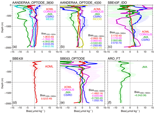
Figure 19 Overall oxygen biases for six oxygen sensor models: (a) AANDERAA_OPTODE_3830, (b) AANDERAA_OPTODE_4330, (c) SBE43F_IDO, (d) SBE43I, (e) SBE63_OPTODE, and (f) ARO_FT. Bias profiles are shown for the six largest DAC datasets (color lines). Values of the average bias for the layer 1000–1900 m (B_{1000–1900 m}) are shown in the lower right part of each panel, with standard errors given in parentheses. Light color shading corresponds to the bias standard error at depth levels, with the number of degrees of freedom equal to the number of distinct Argo floats.

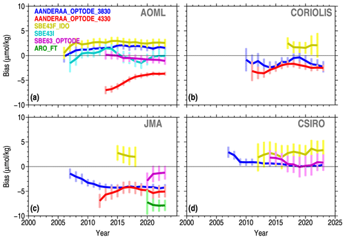
Figure 20 Residual oxygen bias for the layer 1000–1900 m versus time. Vertical bars show standard error with the number of degrees of freedom equal to the number of distinct floats. Each value corresponds to the bias averaged within the 5-year time window. Calculations are shown for the data from distinct DACs: (a) AOML, (b) Coriolis, (c) JMA, and (d) CSIRO.

In order to assess the stability of the overall bias estimates shown in Fig. 19, we calculated time series of the average bias within the layer 1000–1900 m for six most abundant sensor models (Fig. 20). The changes in the diagnosed biases over time indicate a certain degree of sensor stability, with biases typically remaining positive or negative over the entire period of observations. At least part of this apparent time variability may be due to the changes in the number of collocated pairs and their geographical distribution over time. Considering the strong limitation imposed by the number of available collocated pairs, we suggest overall constant bias corrections for different sensors and DACs (Table 4). These corrections correspond to the residual biases in the layer 1000–1900 m (see Fig. 19).

Table 4 Sensor-specific bias corrections for data from different DACs^∗).

^* Bias corrections are given in µmol kg⁻¹. Values in parentheses show standard errors. If the standard error is not shown, the correction indicates a guess value equal to the mean of values with standard error estimate. Corrections indicated in the table should be subtracted from the reported oxygen value. Empty boxes correspond to the sensors which are absent for a specific DAC.

Finally, overall biases were calculated for the data from eight distinct DACs (South Korean datasets from KORDI and KMA are relatively small and do not have collocations with reference cruises available for this study). Biases were calculated for the original data (QC-ed and adjusted by DACs) and for the data corrected for residual biases according to Table 4 (Fig. 21). For all DACs, the suggested bias corrections led to the reduction of the overall bias. AOML, CSIRO, and MEDS data are characterized by a rather constant bias below about 700 m depth. Bias profiles for Coriolis and JMA subsets of data indicate the possible impact of pressure effect on oxygen sensors discussed above. It should be noted that the number of collocated profile pairs differs by 2 orders of magnitude among the eight DACs. In the layer above 1900 m, the AOML data have between 6500–9500 collocated pairs for each depth level, whereas the BODC dataset contributes only with 37 Argo profiles having collocations with reference data. A larger variability of the bias over depth for CSIO and BODC data is most likely explained by the insufficient sample size.

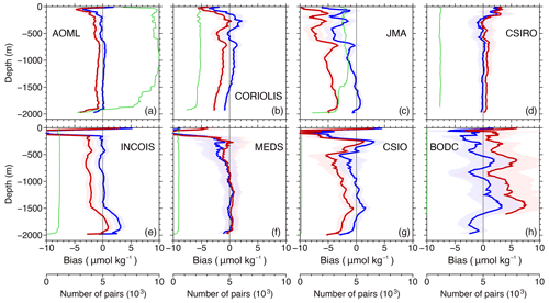
Figure 21 Overall mean Argo oxygen offsets versus Winkler profiles for distinct DACs: (a) AOML, (b) Coriolis, (c) JMA, and (d) CSIRO and (e) INCOIS, (f) MEDS, (g) CSIO, and (h) BODC. Offset profiles for DAC-adjusted data and for the data corrected for residual biases (Table 4) are shown in red and blue, respectively. Standard error bars (light shading) are calculated using the number of distinct floats at each level as the number of degrees of freedom. Green lines show number of collocated pairs in thousands.

6.4 Residual oxygen biases for CTD oxygen sensors

We conducted similar bias calculations for the CTD oxygen profiles obtained by both electrochemical and optical sensors. Only CTD data which passed all QC checks were used for the bias estimation. Unlike Argo profiles, the CTD oxygen sensor data can be adjusted on the simultaneously collected bottles analyzed in the ship laboratory using the Winkler method (Taillandier et al., 2018). Unfortunately, it is not possible to identify profiles with such adjustments within the WOD archive because of missing metadata. As noted by Boyer et al. (2018) “in many cases, the dissolved oxygen … data are uncalibrated and not of high quality. Information on whether these variables are calibrated is not usually supplied by the data submitter”. As noted by Uchida et al. (2010), calibration of oxygen sensor profiles is not straightforward, requires some expertise, and depends on the quality of the reference data. Saout-Grit et al. (2015) described the calibration procedure for SBE 43 sensors done by fitting to reference Winkler data and found a time trend in residuals during the analyzed cruise. WOD archives the data submitted by the data producers and other resources. Thus, the data quality and calibration procedure of the CTD oxygen data are likely inhomogeneous.

For 0–1900 m, we find an overall CTD oxygen offset of about 0.25 µmol kg⁻¹ (median) relative to the Winkler data over the 1960–2022 period, which is much smaller than Argo oxygen biases ranging from −3.72 (JMA) to 0.76 µmol kg⁻¹(CSIRO) (see Fig. 19). Similar to Argo data the offset distribution above 1000 m level (Fig. 22e) exhibits stronger spread than that below 1000 m. The median offset for the layer 1000–2000 m is 0.25 µmol kg⁻¹. Grégoire et al. (2021) indicated that “the uncertainty associated with the last generation of O₂ sensors that uses the best calibration and calculation methods amounts, in the best case, at ∼ 2 µmol kg⁻¹”. Therefore, the overall median offset of 0.25 µmol kg⁻¹ identified by this study is well within the expected uncertainty of the CTD sensors. Besides, there is no spatial uniform pattern for the CTD offsets (Fig. 22d), implying that this offset might not be systematic. Further investigation of the offsets for different cruises (figure not shown) indicates that the offset varies cruise by cruise and year by year. Therefore, in this study, we decided not to adjust the CTD data before the offset can be further confirmed after a cruise-by-cruise investigation and the underlying reasons for the bias can be understood.

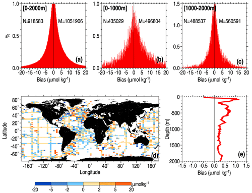
Figure 22 Statistics of the CTD oxygen bias relative to collocated Winkler data. Histograms of layer-averaged bias for 0–2000 m (a), 0–1000 m (b), and 1000–2000 m (c). Number of negative (N) and positive (M) bias values is shown respectively on the left and right side of each histogram. (d) Median of depth-averaged bias (1000–2000 m) in 2°×4° grid boxes and (e) overall median CTD oxygen offset as a function of depth.

7 Impact of quality control and bias adjustment on estimating oxygen changes

Applying the QC and bias adjustment to historical in situ oxygen data is expected to impact the derived ocean oxygen changes on various spatial and temporal scales. To illustrate this impact, we implemented the new Auto-QC system for all oxygen data and adjusted the Argo data based on the approach described in Sect. 6. Based on these data, we applied the mapping method (ensemble optimal interpolation approach with a dynamic ensemble from climate model simulations, EnOI-DE) proposed by Cheng et al. (2017, 2020) to spatially interpolate oxygen data, yielding a spatially complete gridded global ocean oxygen dataset. Because of the limited spatial coverage of oxygen data, we combine each successive 3 years of data to derive oxygen fields for each calendar year. Respectively, the oxygen time series are based on these fields. The reconstruction is only done for the upper 2000 m because of the insufficient in situ data in the abyssal layers. The resultant oxygen field is denoted as “after QC/adjustment”. To show the impact of QC and adjustment on the oxygen changes' estimate, we also applied the same method to the data without QC (e.g., with only several crude QC checks applied to remove most likely erroneous values, including overall range checks, solubility check, and spike check) and without Argo adjustments. The resultant field is denoted as “before QC/adjustment”.

The long-term mean states (e.g., the climatology, reconstructed using all data between 1990–2022 based on the EnOI-DE approach) of the upper 1000 m oxygen before and after QC/adjustment are very similar (Fig. 23a, b). One reason is that the EnOI-DE method (as any mapping approach) has a smoothing effect, so the erroneous data are less visible behind high spatial variability. This indicates the robust large-scale pattern, where the oceans in the low latitudes have lower oxygen concentrations than in the higher latitudes because of the water temperature and ocean circulation difference. The eastern Pacific and north Indian oceans show even lower oxygen levels because of the subsurface oxygen minimum zone. The difference between oxygen climatologies calculated before and after QC/adjustment ranges from −15 to 15 µmol kg⁻¹ but differs at different locations (Fig. 23c). The zonal mean difference is smaller (−3 to 1 µmol kg⁻¹) because of the error cancellation at each latitude (Fig. 23d).

The QC/adjustment also impacts the annual cycle (including both phase and magnitude) of the global mean oxygen changes (Fig. 23e). Examples for the layers 0–100 m (representing the upper seasonal change layer), 100–600 m (representing the main thermocline),, and 0–2000 m (showing the ocean oxygen inventory) are shown in Fig. 23e. For 0–100 m, the mean oxygen level shifts from negative to positive in November after QC/adjustment but in September before QC/adjustment. The magnitude of the annual cycle (defined as the difference between the maximum and minimum of the 12-month climatology time series) is 1.45 µmol kg⁻¹ but slightly reduced after QC/adjustment (1.22 µmol kg⁻¹). Similarly, the annual cycle magnitude for the layers 100–600 and 0–2000 m reduced from 1.18 and 0.55 µmol kg⁻¹ before QC/adjustment to 0.79 and 0.48 µmol kg⁻¹ after QC/adjustment (Fig. 23e).

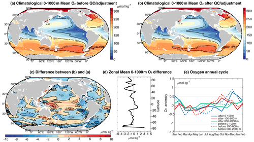
Figure 23 The climatological upper 1000 m oxygen field before (a) and after (b) QC/adjustment, with their spatial difference shown in (c) and zonal mean differences in (d). The annual cycle (relative to the climatological annual mean level) before (dashed line) and after (solid line) QC/adjustment are compared in (e) for different vertical layers. The climatology field is reconstructed by combining all data within 1990–2022 with EnOI-DE mapping method (Cheng et al., 2017, 2020).

The QC and adjustment also impact the estimates of long-term oxygen changes, for example the global deoxygenation estimates for 0–100, 100–600 and 0–2000 m layers depicted in Fig. 24. After QC/adjustment, the standard deviation of the time series is decreased from 1.71 (0–100 m), 2.37 (100–600 m), and 1.60 (0–2000 m) to 1.62 (0–100 m), 2.24 (100–600 m), and 1.44 (0–2000 m) µmol kg⁻¹, showing a reduced variability in global oxygen time series after QC/adjustment. This indicates a reduction of noise, which is mainly attributed to both QC and Argo adjustment. For example, before QC/adjustment, there was a big global deoxygenation of ∼ 3 µmol kg⁻¹ from 1995 to 1996 in the layer 0–100 m, which is likely non-physical and spurious. This feature disappeared after QC/adjustment (Fig. 24). The linear rate of deoxygenation differs for the two test changes as well: −0.77 ± 0.43 (0–100 m), −1.45 ± 0.30 (100–600 m), and −0.95 ± 0.30 (0–2000 m) µmol kg⁻¹ per decade before QC/adjustment and −0.90 ± 0.38 (0–100 m), −1.37 ± 0.40 (100–600 m), and −0.84 ± 0.41 (0–2000 m) µmol kg⁻¹ per decade after QC/adjustment. The linear trend is calculated by the ordinary least-squares regression with a 90 % confidence interval shown (accounting for the reduction in degree of freedom). The deoxygenation rates are reduced after QC/adjustment for both 100–600 and 0–2000 m, mainly because of the Argo adjustment, which shifted the oxygen level in the past decade by ∼ 0.76 µmol kg⁻¹ for 100–600 m average and ∼ 0.82 µmol kg⁻¹ for 0–2000 m average within 2015–2023 (Fig. 24).

By means of these tests we demonstrate that QC and bias adjustment can impact the estimation of the oxygen changes at various temporal–spatial scales, highlighting the need for a careful oxygen data processing before application. However, we note here that the validity of the mapping approach on oxygen reconstruction has not been thoroughly evaluated, which deserves a separate study.

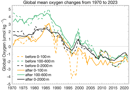
Figure 24 The reconstructed global averaged oxygen time series before (dashed line) and after (solid line) QC/adjustment from 1970 to 2023 for the layers 0–100, 100–600, and 0–2000 m. Here, we combine each successive 3 years of data to estimate the oxygen changes. The anomalies are calculated relative to the climatology shown in Fig. 23.

8 Data availability

The quality control procedure described above was applied to the OSD and CTD oxygen profiles between 1920 and 2023 from the World Ocean Database (https://www.ncei.noaa.gov/access/world-ocean-database-select/dbsearch.html, Mishonov et al., 2023) and to the oxygen profiles from the BGC Argo floats (https://doi.org/10.17882/42182, Argo, 2024). The resulting dataset comprises observed level data with quality flags and data interpolated on 10 m levels. The data are in NetCDF format and include metadata information. The complete dataset (Gouretski et al., 2024) can be found at https://doi.org/10.12157/IOCAS.20231208.001 and http://www.ocean.iap.ac.cn/ftp/cheng/IAP_oxygen_profile_dataset (last access: 26 November 2024).

9 Code availability

The code of the QC system developed in this paper is available at http://www.ocean.iap.ac.cn/ftp/cheng/IAP_oxygen_profile_dataset/QC_Code_SAMPLE.zip (Gouretski et al., 2024).

10 Conclusion and discussion

This study developed a new automated QC scheme for ocean oxygen profile data and applied it to the OSD and CTD oxygen profiles from the WOD and to the Argo float oxygen profiles provided by national DACs. The procedure consists of 10 quality checks based on local or global parameter thresholds. Some checks are conceptually similar to the quality checks used to validate the profiles in the World Ocean Database (Boyer et al., 2018) (for example, the global range test and vertical gradient test) and in the Argo Data Acquisition Centers (Thierry et al., 2021) (for example, spike and “frozen” profile tests). However, we provide additional checks (for example, test for the number of local extrema and local climatological range test), which increase the ability of the QC procedure to better identify erroneous data. For instance, the procedure proves whether an oxygen value falls out of accepted ranges (defined by globally or locally) or whether an oxygen profile exhibits a very untypical shape. The shape of the profile is characterized by the vertical oxygen gradient, by the number and magnitude of local oxygen extrema, and by the presence of spikes. The check is also done for the so-called “frozen” profiles occurring when the oxygen sensor sticks and reports the same values throughout the profile.

The QC procedure presented here is tailored for the quality assessment of the archived oxygen data obtained by both Winkler methods and sensors. Large ocean depositories like WOD often contain observed data that have already undergone a certain degree of QC and adjustment. Therefore, our QC procedure differs from the real-time QC of dissolved oxygen observations by means of oxygen sensors as suggested in the frame of the Integrated Ocean Observing System (IOOS) in the quality control manual by Bushnell et al. (2015) (B2015 hereafter). Three quality tests which have been required or suggested in that manual can only be applied to real-time data: the application of the gap test needs the time stamp of each measurement, the application of the syntax test requires the full original data record, and the application of the neighbor test is only possible in the case when a nearby second sensor is installed on the device. Information needed for these tests is not kept in the WOD; therefore these tests cannot be applied to “static” archive data. Five other tests outlined in B2015 are conceptually similar to the tests applied by our QC procedure: location test, gross range test, climatology test (all three required by B2015), spike test, and flat line test (both recommended by B2015). In a deviation from our QC procedure, thresholds for test variables according to B2015 should be chosen subjectively by operators in the data centers. We note that the metadata on decisions made operators are usually missing in the data archives.

The novelty of the proposed quality scheme is that the threshold choice is based on the respective statistics of test variables, and the Gaussian distribution is not assumed for the important local climatological range checks for oxygen and for oxygen vertical gradient. The QC procedure presented in this study was benchmarked against several hydrographic datasets known for their outstanding measurement quality, with WOCE experiment data collection being the largest and best documented. Analysis of the outliers and their distribution among distinct hydrographic sections and cruises suggests the ability of the procedure to flag outliers but retain the overwhelming majority of good data. The accompanying diagnostic tool provides the overview of outlier scores and permits tuning of thresholds when new benchmark quality-controlled datasets become available. Finally, we note that the transparent choice of test threshold values on the basis of the underlying statistics and the subsequent analysis of outliers for each quality check permits further tuning of the quality control procedure in order to increase the percentage of true outliers and to decrease the percentage of falsely identified outliers.

Further, we estimated possible residual oxygen biases in the delayed-mode adjusted Argo oxygen profiles. The bias estimates are based on the collocated Argo and discrete water sample ship-based profiles. The latter represents reference measurements as the bottle samples are analyzed by means of the Winkler chemical method. The size of the collocation bubble (e.g., the maximum distance between two profiles and the maximum time difference) was set at 100 km and 5 years, respectively, after several experiments with different bubble sizes. Residual biases relative to the Winkler reference data are represented by the difference at an isobaric level between the Argo sensor oxygen value and the Winkler oxygen, with the overall bias at each level being defined by the average of individual differences. To reduce the impact of time- and spatial variability, the final bias assessment is done for the layer 1000–1900 m, which is typically located below the main thermocline.

Using all available Argo profiles which have collocations with reference Winkler data, we calculated overall oxygen offsets for six models of oxygen sensors implemented on Argo BGC floats and for six Argo DACs. Our results suggest that derived biases are both sensor- and DAC-specific, with the electrochemical SBI-series sensors exhibiting a positive bias in the range from 0.5 to 2.6 µmol kg⁻¹. The optode sensors typically are characterized by negative biases ranging between −0.7 and −6.2 µmol kg⁻¹ depending on sensor model and DAC. Only for AANDERAA_OPTODE_3830 were small positive offsets found for AOML and CSIRO, as well as positive offsets for SBE63_OPTODE for Coriolis and CSIRO. These diagnosed biases are crucial to accurately identify the deoxygenation trend, as current assessments suggest an upper 1000 m O₂ content decrease of 0.2–1.2 µmol kg⁻¹ per decade during 1970–2010 (Gulev et al., 2021). Our calculations suggest that at least 1000 collocation pairs are needed for the stable residual bias estimation. This number of collocations is available only for AOML, Coriolis, JMA, CSIRO, INCOIS, and MEDS datasets.

Diagnosed residual biases for the quality-controlled CTD oxygen sensor profiles revealed a good agreement between the CTD and Winkler reference data, with a small median bias of 0.25 µmol kg⁻¹ within the layer below 1000 m. Because of a relatively small bias value, which is well within the uncertainty of the CTD sensors and due to a non-uniform spatial CTD bias pattern, the diagnosed overall bias is not considered to be a common and robust feature, and no adjustment of CTD data is performed in this study. Our preliminary investigation also indicates that the CTD offset varies cruise by cruise, probably associated with the differences in the calibration or re-calibration (or post-processing). Therefore, the follow-on work should include investigating the offsets on a cruise-by-cruise basis and providing an understanding of the causes of bias. Only after these examinations are done can the adjustment of CTD profiles be physically tenable.

This study also has some limitations and caveats:

1. Although systematical errors have been identified for Argo oxygen data, the cause of the biases is still poorly known and requires further work. The differences between the DACs are also mysterious, and we suspect that the non-standard adjustment procedure developed by different National Argo Data Centers and the difference in sensors on Argo floats used in different countries might be responsible for the differences in diagnosed biases, which needs further confirmation.

2. Because the sources of biases are poorly known, the correction proposed in our study is largely empirical and can be applied only to the Argo data used in this study. If the Global Argo Data Center updates quality control and adjustment procedures, our bias corrections also require an update.

3. The QC procedure is designed to detect and flag the outliers. However, there are also risks of removing the “real extremes” in the ocean, especially under rapid climate change, as ocean extreme events are expected to become more frequent. One possible way to partly resolve this problem is imposing a trend in the local climatological range, accounting for the time variation of the local oxygen distributions due to climate change, which would help to reduce the false rejection of the real extreme data. This requires further work when the local oxygen trends become clearer.

4. The Winkler data are used in this study as a reference. However, it is likely that the Winkler data are not always taken to the same standard, thus posing inconsistency within the Winkler dataset, especially for the data taken by different countries and in different time periods. Investigating offsets on a cruise-by-cruise basis is also recommended in the future, as for CTD data.

In summary, this study proposed a new quality control approach and bias assessment for the CTD, bottle, and Argo oxygen data and investigated the consistency between these three primary instrumentation types. Our investigations ensured the consistency between the three data types and provided a solid basis for merging them into a single, integrated, and homogeneous oxygen database. Therefore, the database obtained in this study supports the next-step assessment and understanding of the change in ocean oxygen levels.