Spatio-temporal changes in China's mainland shorelines over 30 years using Landsat time series data (1990–2019)

Continuous monitoring of shoreline dynamics is essential to understanding the drivers of shoreline changes and evolution. A long-term shoreline dataset can describe the dynamic changes in the spatio-temporal dimension and provide information on the influence of anthropogenic activities and natural factors on coastal areas. This study, conducted on the Google Earth Engine (GEE) platform, analyzed the spatio-temporal evolution characteristics of China's shorelines, including those of Hainan and Taiwan, from 1990 to 2019 using a long time series of Landsat Thematic Mapper (TM), Enhanced Thematic Mapper Plus (ETM+), and Operational Land Imager (OLI) images. First, we constructed a time series of the modified normalized difference water index (MNDWI) with high-quality reconstruction by the harmonic analysis of time series (HANTS) algorithm. Second, the Otsu algorithm was used to separate the land and water of coastal areas based on MNDWI value at high-tide levels. Finally, a 30-year shoreline dataset was generated and a shoreline change analysis was conducted to characterize length change, area change, and rate of change. We concluded the following: (1) China's shoreline has shown an increasing trend in the past 30 years, with varying growth patterns across regions; the total shoreline length increased from 24 905.55 km in 1990 to 25 391.34 km in 2019, with a total increase greater than 485.78 km, a rate of increase of 1.95 %, and an average annual increasing rate of 0.07 %. (2) The most visible expansion has taken place in Tianjin, Hangzhou Bay, and Zhuhai for the three economically developed regions of the Bohai Bay–Yellow River estuary zone (BHB-YREZ), the Yangtze River estuary–Hangzhou Bay zone (YRE-HZBZ), and the Pearl River estuary zone (PREZ), respectively. (3) The statistics of shoreline change rate for the three economically developed regions show that the average end point rates (EPRs) were 43.59, 39.10, and 13.42 m yr⁻¹, and the average linear regression rates (LRRs) were 57.40, 43.85, and 10.11 m yr⁻¹, respectively. This study presents an innovative and up-to-date dataset and comprehensive information on the status of China's shoreline from 1990 to 2019, contributing to related research and policy implementation, especially in support of sustainable development (https://doi.org/10.57760/sciencedb.16228, Yang et al., 2024).

1 Introduction

A shoreline, the boundary between sea and land, represents an important geographical element of a coastal area and a vital component of land resources. It has been identified as one of the 27 features recognized by the IGDC (International Geographic Data Committee) (Kuleli et al., 2011). As marine development expands, a shoreline plays a crucial role in protecting the environment and maintaining the ecological balance of coastal zones. Since the 20th century, the economic center of gravity of coastal countries has gradually shifted toward coastal areas, and, currently, nearly 50 % of the world's population lives within 100 km of the shoreline (Li et al., 2018). The shift in the center of economic development has led to major changes in shoreline resources, impacting the economic, social, ecological (Yang et al., 2022), and environmental aspects of coastal areas (Sui et al., 2020). The intensification of human exploitation and the shrinking of shoreline resources in nearshore areas has resulted in increasing tensions between the exploitation and protection of shorelines (Liu et al., 2018). Therefore, understanding the current coastal resource development plays an important role in regional sustainable development.

Accurate and rapid extraction of shoreline information is key to shoreline research. In long-term shoreline monitoring, traditional manual field measurement methods tend to be impractical as they are time-consuming, inefficient, expensive, and easily restricted by complex geographical environment conditions (Liang et al., 2018). In comparison, remote sensing has the advantages of wide coverage (Li and Gong, 2016), short revisit period, and low acquisition costs (Mao et al., 2020). Therefore, remote sensing has gradually become an important piece of technology for shoreline monitoring. Shoreline extraction methods can be divided into visual interpretation and automatic extraction (Toure et al., 2019; Mao et al., 2022; Bishop-Taylor et al., 2021). Visual interpretation mainly relies on human–computer interaction to identify shorelines based on remote sensing image interpretation, but it heavily depends on the expertise of the interpreter and is easily influenced by subjective factors. Therefore, it is not suitable for large-scale and long-term shoreline information extraction. Automatic extraction methods utilize spectral feature differences to identify shorelines. Compared to the visual interpretation method, automatic extraction methods have better universality and timeliness, making them an important means of shoreline remote sensing extraction (Chen et al., 2022; R. Hu et al., 2021).

Remote-sensing-based methods for automatic interpretation of shoreline information extraction encompass a range of techniques, including threshold segmentation, edge detection, image classification, active contour models, and object-oriented and deep learning approaches (Aedla et al., 2015; Wang et al., 2017; Yancho et al., 2020; Wei et al., 2021; Liang et al., 2023). The threshold segmentation method involves setting a threshold based on the difference in values in greyscale between the target and background pixels to segment the waterbodies (Hu and Wang, 2022; Wang et al., 2020). This method is characterized by its simplicity, efficiency, and ease of implementation (Dai et al., 2019). However, similarities in spectral features can limit its effectiveness when dealing with pixels exhibiting similar characteristics (Wang et al., 2017; Mao et al., 2021). The edge detection method directly extracts the edge information of the shoreline by identifying pixels with a significant step change in greyscale values using edge detection operators (Karantzalos et al., 2002). While this method performs well for regular shorelines, it is sensitive to noise in complex shoreline image backgrounds, resulting in poor continuity of the extracted shorelines (Toure et al., 2019). The image classification method utilizes various features such as the spectrum, texture, and shape of the image to construct feature vectors, which are then used to train classifiers for region classification and shoreline extraction (Tang et al., 2022; Otukei and Blaschke, 2010). This approach is straightforward and effective; however, it requires meticulous feature selection and high-quality image data. The active contour model method consists of the edge active contour model and the region active contour model (Abdelsamea et al., 2015; Paragios and Deriche, 2000). It leverages the gradient information of the image edges or the overall greyscale information of the region to accurately extract the shoreline (Zhang et al., 2013; Liu et al., 2017; Airouche et al., 2009). Nevertheless, this method entails complex models, computationally intensive processes, and time-consuming extraction procedures. The object-oriented method integrates spectral, spatial, and textural features of remote sensing images to segment waterbodies and land, with the object as the target, facilitating shoreline information extraction (Wang et al., 2023; Pekel et al., 2016; Apostolopoulos and Nikolakopoulos, 2020). This method achieves high accuracy in shoreline extraction but requires complex parameter settings, which may lead to the loss of valuable information in complex datasets (Ge et al., 2014). Deep learning methods construct models that can automatically identify shorelines by learning image features and contextual information from sample data (Seale et al., 2022; Dang et al., 2022; Dai et al., 2019). This approach has been shown to be able to reliably predict complex shorelines. However, training deep learning models is difficult and necessitates large amounts of pure sample data (Chen et al., 2019).

Wu et al. (2014) utilized topographic maps and remote sensing images collected at various time points spanning from 1940 to 2012 to define and calculate the index of shoreline utilization degree for mainland shorelines at national, provincial, and local scales. Similarly, Li et al. (2023) selected Landsat series images from five time periods (1990–2020) to monitor and analyze various shoreline characteristics, such as shoreline length, sea and land patterns, shoreline diversity index, and fractal dimension. However, most existing long-term analyses of large-scale shoreline changes used remote sensing images acquired at several time points (e.g., monitoring intervals of 5 or 10 years) (Rahman et al., 2011; Murray et al., 2014). This limited monitoring frequency often led to missing information on continuous changes and an inaccurate representation of fine change characteristics of the shoreline. Given these limitations and recognizing the influence of tides on shoreline extraction as well as the highly dynamic nature of shorelines, a long-time-series water index dataset was derived by exploiting the availability of large Earth datasets. The methodology included water index time series reconstruction, threshold segmentation, and Digital Shoreline Analysis System (DSAS). These techniques enabled the automatic extraction of long-time series of shoreline maps and facilitated the analysis of spatio-temporal evolution characteristics of large-scale shorelines.

2 Study area and materials

2.1 Study area

The coastal zone of China extends from the estuary of the Yalu River on the China–North Korea border in the north to the mouth of the Beilun River on the China–Vietnam border in the south (Wang et al., 2023; Y. Hu et al., 2021). The seas of China include the Bohai Sea, Yellow Sea, East China Sea, and South China Sea (Qin et al., 2023). They span 14 provinces, municipalities, and autonomous regions, including Liaoning, Tianjin, Hebei, Shandong, Jiangsu, Shanghai, Zhejiang, Fujian, Guangdong, Guangxi, Hainan, Hong Kong SAR, Macao SAR, and Taiwan (Fig. 1). The Bohai Bay–Yellow River estuary zone (BHB-YREZ), the Yangtze River estuary–Hangzhou Bay zone (YRE-HZBZ), and the Pearl River estuary zone (PREZ), are part of the Bohai Economic Rim, the Yangtze River Delta Economic Zone, and the Pearl River Delta Economic Zone, respectively – the three fastest-growing economic regions, which are also the most urbanized areas in China (Wang et al., 2021). It includes three climate zones: temperate, subtropical, and tropical zones, with an average annual temperature of 5 to 25 °C and an average annual precipitation of 400 to 1800 mm (Mao et al., 2019).

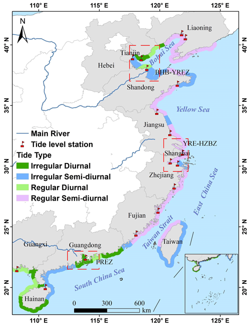
Figure 1 Location of China's coastal zone and spatial distribution of tide-level stations and tide types.

The coast of China is bounded by Hangzhou Bay, with silty shorelines in the north and bedrock shorelines in the south. Most coastal areas are flat and low-lying, with an average elevation of 2–5 m, and are vulnerable to erosion by sea level rise (Yin et al., 2012). At present, more than 40 % of China's population lives in coastal provinces, which account for 15 % of the country's land area (Wang et al., 2014). In the past 30 years, these regions' gross domestic product (GDP) has maintained a growth rate of more than 7 %, accounting for more than 57 % of national revenue (Tian et al., 2016; SOA, 2015). However, a series of economic activities in coastal areas have also exerted extensive and profound impacts. Reclamation, aquaculture, construction of seawalls, and development of ports and harbors have significantly influenced the environment and biodiversity of coastal regions. These human activities have resulted in shoreline alterations, wetland ecosystem degradation, and marine pollution (Tiner, 2013; Meng et al., 2017).

2.2 Landsat data

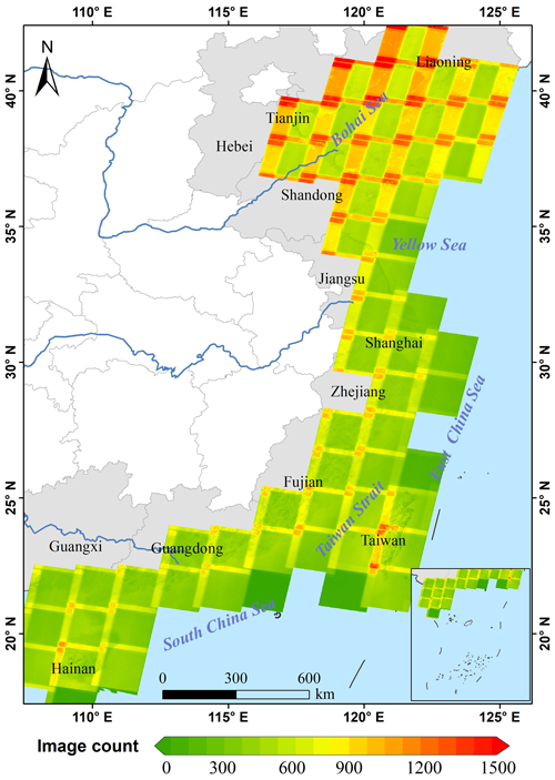
The study area covers 57 tiles (paths/rows) of the Landsat Worldwide Reference System (WRS-2) (Fig. 2). All the available level 1 Terrain-corrected (L1T) orthorectified Landsat surface reflectance images for the period 1990–2019, including Thematic Mapper (TM), Enhanced Thematic Mapper Plus (ETM+), and Operational Land Imager (OLI), were retrieved. A total of 60 527 Landsat images (Fig. 1b) were archived on the Google Earth Engine (GEE) platform as a US Geological Survey (USGS) image set. The quality assessment (QA) band, which contains cloud information, was used to mask bad-quality observations caused by clouds, cirrus clouds, and cloud shadows in each image (H. Li et al., 2019; Wang et al., 2020). For the mudflat area greatly affected by the tide, we screened the Landsat image closest to the high tide according to the high-tide time of the tide station and the imaging time of the satellite image.

Figure 2 Landsat TM/ETM+/OLI image coverage of good-quality observations from 1990 to 2019.

2.3 Auxiliary data

2.3.1 Tidal data

To study the influence of tides on shorelines, we selected 17 key tidal stations, including eight stations in the warm temperate zone, seven stations in the subtropical zone, and two stations in the tropical zones (Jia et al., 2021). These stations are located on coasts of different tidal types and are adjacent to large tidal flat areas. Tidal tables of these stations are available online (https://www.chaoxibiao.net/, last access: 12 November 2024). To eliminate the influence of precipitation, we selected the tidal data for the rainy season in China's coastal zone, which spans from April to September (Liu et al., 2018). Based on high-tide times and satellite transit times, 1583 images were selected to extract the shoreline. These tide site locations are summarized in Table 1.

Table 1 General information on tide stations (from north to south).

2.3.2 Reference datasets

This study used three global shoreline datasets as reference datasets. Table 2 lists their general information. A new global shoreline vector (GSV; Sayre et al., 2019) with a spatial resolution of 30 m was developed from annual composites of 2014 Landsat satellite imagery. The semi-automated classification of the imagery involved manually selecting training points representing water and non-water classes along the entire global shoreline. The 2015 Global Multiple Scale Shorelines Dataset (GMSSD_2015; Liu et al., 2019) was generated using Google Earth imagery. This dataset includes the global vector shoreline data with meter-level resolution, which was obtained through human–computer interaction and analysis of Google Earth images. Coastline_ECS (Li et al., 2019) is a dataset of spatio-temporal change in continental shorelines and their types for the East China Sea region. The dataset covers 5-year intervals from 1990 to 2015 and was generated using Landsat images through the application of a single-band edge detection method, which selected three time points from the dataset: 1990, 2000, and 2015.

Table 2 Datasets used to evaluate the accuracy of shoreline position.

3 Methodology

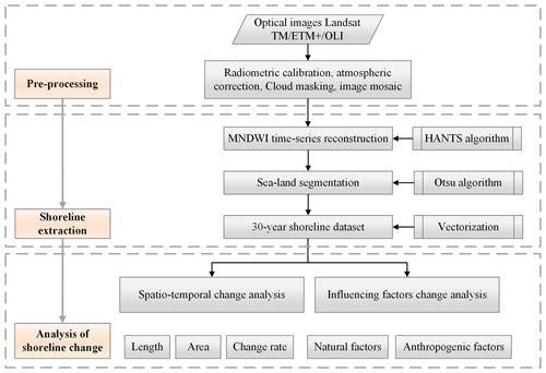
To accurately monitor the temporal and spatial dynamic changes in China's shoreline, this study utilized medium-resolution remote sensing imagery data from 1990 to 2019 and applied a threshold segmentation method based on exponential time series reconstruction. This method effectively extracts long time series of shoreline information and carries out shoreline temporal and spatial evolution analysis. The framework of the study is shown in Fig. 3.

Figure 3 Framework for mapping shoreline changes.

3.1 Extraction of shoreline using remote sensing images

Multi-band Landsat satellite data were utilized to calculate the modified normalized difference water index (MNDWI) to distinguish between water and non-water pixels. This method generates outputs that can accurately map shorelines at the pixel level. Previous research has demonstrated that the MNDWI index outperforms the NDWI index for shoreline extraction (Xu, 2006; Lin et al., 2020). The formula for calculating the MNDWI index is as follows:

$$\begin{array}{}\text{(1)}& \text{MNDWI}=\left(\text{green}-\text{MIR}\right)/\left(\text{green}+\text{MIR}\right),\end{array}$$

where green represents the reflectance of the green light band and MIR represents the reflectance of the mid-infrared band, corresponding to B2 and B5 of Landsat TM/ETM+ images, and B3 and B6 of Landsat OLI images, respectively.

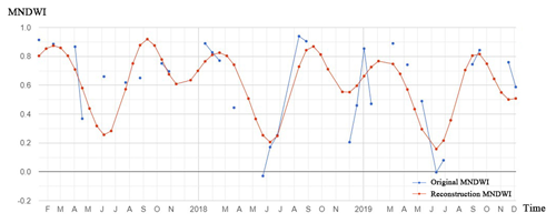
Disturbances in the time series of MNDWI were due to the influence of cloud coverage. To remove outliers without distorting the original shape and features of the data (Cao et al., 2020), the harmonic analysis of the time series (HANTS) algorithm was adopted to construct high-quality data in this study (Zhou et al., 2015). The HANTS algorithm involved several steps: firstly, the removal and smoothing of noises in time series observation and, secondly, the filling of missing values in time series observations through interpolation (Fig. 4). HANTS is an improved algorithm based on the fast Fourier transform, which realizes outlier discrimination and missing value filling through a Fourier transform and least-squares fitting.

Figure 4 The application of the HANTS algorithm to an example pixel from our study area.

The Otsu algorithm (Otsu, 1979) is an adaptive thresholding method. basic principle is to find the optimal threshold for segmenting an image using the least-squares method. It categorizes all elements of an image into two classes (Ding et al., 2021): background pixels and target pixels. It calculates the between-class variance by utilizing the greyscale histogram of the segmented image. The threshold is then found by maximizing the between-class variance (or, in other words, by minimizing the within-class variance) (Donchyts et al., 2016). In this paper, greyscale MNDWI images were segmented into waterbodies and non-waterbodies using the Otsu threshold segmentation technique. The Otsu thresholding was performed separately for each year, leading to potentially different thresholds being used for each annual time step.

In the process of extracting waterbody information, it is necessary to exclude pixels corresponding to lakes and reservoirs. Coastal waterbodies resulting from the aforementioned process may contain lakes, reservoirs, and similar features due to their distinct shapes and comparable sizes. The fundamental distinction between lakes, reservoirs, and oceans lies in their geographic distribution and area sizes. Lakes and reservoirs are dispersed, whereas oceans are concentrated and contiguous. Thus, this study employed an area parameter to effectively eliminate interference caused by terrestrial waterbodies. By selecting the largest waterbody area for each object, the marine area can be accurately delineated. Moreover, as image resolution can introduce jagged artifacts, converting raster data into a vector format may result in shoreline boundaries that exceed their true length. To address this issue, the Smooth Line tool was utilized to mitigate the jagged artifacts and obtain a refined representation of the shoreline data.

3.2 Consistency test

Due to confidentiality reasons, we are unable to obtain and publicly display the measured data of the coastline for accuracy verification. On the other hand, it is difficult to match our results to the measured shoreline data from the management department in terms of definition and resolution. Therefore, we adopt consistency testing with the reference dataset instead of using actual data for accuracy verification. Three shoreline reference datasets were utilized to compare the results of shoreline extraction – namely, CSV, CMSSD_2015, and Coastline_ECS. Specifically, shoreline data from 1990, 2000, 2014, and 2015 were compared with CSV_2014, CMSSD_2015, Coastline_ECS_1990, Coastline_ECS_2000, and Coastline_ECS_2015, respectively. To evaluate the consistency of shoreline extraction results, 2804, 2716, 741, 742, and 743 points were randomly generated using the CSV_2014, CMSSD_2015, Coastline_ECS_1990, Coastline_ECS_2000, and Coastline_ECS_2015 datasets, respectively. The offset (without distinguishing between inland or seaward biases) and mean absolute deviation were then calculated using the following formulas:

$$\begin{array}{}\text{(2)}& \text{offset}=D_n,\end{array}$$

$$\begin{array}{}\text{(3)}& \begin{array}{rl}\stackrel{\mathrm{‾}}{d}& ={\displaystyle \frac{\left|D_{\mathrm{1}}-\stackrel{\mathrm{‾}}{D}\right|+\left|D_{\mathrm{2}}-\stackrel{\mathrm{‾}}{D}\right|+\mathrm{\cdots }+\left|D_n-\stackrel{\mathrm{‾}}{D}\right|}{n}}\\ & ={\displaystyle \frac{{\sum }_{i=\mathrm{1}}^n\left|D_i-\stackrel{\mathrm{‾}}{D}\right|}{n}},\end{array}\end{array}$$

where the offset is defined as the distance between shorelines, n is the number of sample points, D is the nearest-neighbor distance between feature points in the reference shoreline dataset and the extracted shoreline, $\stackrel{\mathrm{‾}}{D}$ is the average nearest-neighbor distance, and $\stackrel{\mathrm{‾}}{d}$ is the mean absolute deviation.

3.3 Dynamic change analysis of shoreline

We calculated the shoreline length for each year in ArcGIS 10.4 using the Geometry tool. To analyze changes in area, we selected the 1990 shoreline as our baseline. The area included between shorelines was calculated to determine the change in area resulting from erosion and accretion.

We employed the Digital Shoreline Analysis System (DSAS) (Baig et al., 2020; Thieler et al., 2009), an ArcGIS extension developed by the USGS, to calculate the spatio-temporal change rate of the shoreline. First, we created a 500 m buffer using the 1990 shoreline and simplified and manually edited it to generate a baseline. Then, perpendicular transects, spaced at intervals of 500 m, were traced relative to the baseline. These transects intersected with the shoreline, establishing measurement points. Finally, the change rate of the shoreline was calculated from the distances between the baseline and each intersection point.

In this paper, the end point rate (EPR) and the linear regression rate (LRR) equations were used to calculate the shoreline change rates (Eqs. 4–7).

$$\begin{array}{}\text{(4)}& \text{EPR}={\displaystyle \frac{\text{NSM}}{\text{SP}}},\end{array}$$

where net shoreline movement (NSM) is equal to the distance between the oldest and youngest shoreline; the time span (SP) equals the time between the oldest and most recent shoreline measurement.

The statistics of linear regression change rate can be determined by fitting the least-squares regression line to all shoreline points of the transect. LRR can be calculated as the slope of a straight line (Eq. 6). The linear regression method uses all data without considering changes in trend or accuracy (Zhu et al., 2021).

$$\begin{array}{}\text{(5)}& {\displaystyle }y=a+bx,\text{(6)}& {\displaystyle }b={\displaystyle \frac{{\sum }_{i=\mathrm{1}}^n\left(x_i-\stackrel{\mathrm{‾}}{x}\right)\left(y_i-\stackrel{\mathrm{‾}}{y}\right)}{{\sum }_{i=\mathrm{1}}^n{\left(x_i-\stackrel{\mathrm{‾}}{x}\right)}^{\mathrm{2}}}},\text{(7)}& {\displaystyle }a=\stackrel{\mathrm{‾}}{y}-b\stackrel{\mathrm{‾}}{x},\end{array}$$

where x and y are the independent variables of the year and the spatial position of the shoreline, respectively; x_i is the ith year; y_i is the distance from the intersection of the ith profile with the shoreline to the baseline; $\stackrel{\mathrm{‾}}{x}$ and $\stackrel{\mathrm{‾}}{y}$ are the average values of x_i and y_i, respectively; a is the intercept of the fitting constant; and b is the regression slope, which is LRR.

4 Results and analysis

4.1 Consistency test results

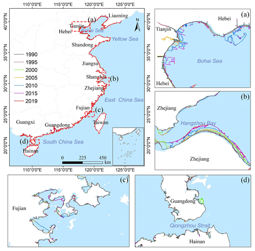
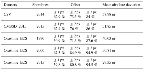
The shorelines mapped from 1990 to 2019 by applying the algorithm proposed in this paper are depicted in Fig. 5. We evaluated the consistency between the extracted coastline and the reference dataset. The results show that the offset of more than 50 % of sample points was less than 1 px. For more than 70 % of sample points, the offset was less than 2 px, and for over 80 % of sample points, it was less than 3 px. The maximum average absolute deviation in shorelines was 57.98 m, while the minimum average absolute deviation was 29.35 m (Table 3). The shoreline extracted by this method has good consistency with the reference dataset, which, to some extent, confirms the reliability of our results.

Figure 5 Spatial distribution of the shoreline during the study period from 1990 to 2019.

Table 3 Consistency test of shoreline information extraction.

4.2 Temporal characteristics evolution analysis

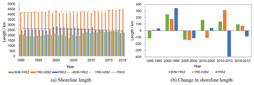
We calculated the shoreline length in ArcGIS 10.4 using the Geometry tool. The length and change in the total shoreline in the study area are shown in Fig. 6. From 1990 to 2019, the shoreline length shows varying degrees of dynamics but generally exhibits a slow growth trend. The shoreline length increased from 24 905.55 km in 1990 to 25 391.34 km in 2022, resulting in a total increase of 485.783 km. This represents a growth rate of 1.95 %, with an average annual growth rate of only 0.07 %. The shoreline length showed alternating increases and decreases from 1990 to 2019, with decreases in 1990–1995, 2000–2005, and 2015–2019 and increases in 1995–2000, 2005–2010, and 2010–2015. The smallest reduction in shoreline length took place from 1990 to 1995, when it decreased by 272.533 km. The most significant reduction in shoreline length took place from 2000 to 2005, dropping from 25 328.036 km in 2000 to 24 445.252 km in 2005, resulting in a decrease of 882.784 km. The period 2010–2015 witnessed the fastest growth in China, with an increase of 957.80 km in shoreline length, followed by the period 1995–2000, with 695.02 km of shoreline length growth. Conversely, the period 2005–2010 experienced the least growth, with only 301.38 km in shoreline length growth.

Figure 6 (a) Length and (b) change in China's shoreline from 1990 to 2019.

Typical regional shoreline lengths and their changes are shown in Fig. 7. From 1990 to 2019, the three economically developed coastal regions show different trends in shoreline length. Among them, the shoreline of BHB-YREZ increased the most, by 392.99 km, with an average annual increase of about 13.10 km. This was followed by YRE-HZBZ, with a total increase of 324.20 km, averaging about 10.81 km annually. In contrast, the shoreline length of PREZ had a significant downward trend, with a decrease of 178.85 km and with an average annual decrease of about 5.96 km.

Figure 7 Regional shoreline length (a) and change (b) from 1990 to 2019.

The change in shoreline length over different periods is shown in Fig. 7b. From 1990 to 1995, the shoreline of BHB-YREZ showed a decreasing trend, while other regions showed an increasing trend. The shoreline of BHB-YREZ decreased by 115.94 km, while PREZ showed the most pronounced increase, extending by 33.68 km. Between 1995 and 2000, the changing trends in shorelines were consistent across regions, showing a significant increase. The BHB-YREZ shoreline increased by 628.66 km, YRE-HZBZ increased by 178.30 km, and PREZ increased the most, extending by 343.63 km. From 2000 to 2005, the shorelines of the three regions showed a decreasing trend. The YRE-HZBZ shoreline decreased the most, retreating by 142.64 km, followed by a 137.40 km reduction in BHB-YREZ, while PREZ decreased by 114.87 km. During this period, the change in shoreline length between the three economically developed regions showed minimal differences. From 2005 to 2010, the shoreline of BHB-YREZ and PREZ showed an increasing trend, while the shoreline of YRE-HZBZ showed a decreasing trend. The shoreline of BHB-YREZ increased by 161.89 km, while YRE-HZBZ decreased the most, by 109.41 km. From 2010 to 2015, PREZ showed a decreasing trend, while others showed an increasing trend. Among them, the shoreline of PREZ decreased by 393.62 km, showing the most significant decreasing trend. Compared with other periods, the largest increase in the length of the shoreline from YRE-HZBZ in this period was 312.59 km. From 2015 to 2019, the shorelines of BHB-YREZ and YRE-HZBZ showed increasing trends, while the shoreline of PREZ showed a decreasing trend. The shoreline of BHB-YREZ increased the most (96.57 km). From the perspective of the entire 30-year period, the changing trend of the shoreline of BHB-YREZ was the most significant from 1995 to 2000. From 2010–2015, the most significant changes were in YRE-HZBZ and PREZ shoreline length.

4.3 Spatial characteristics evolution analysis

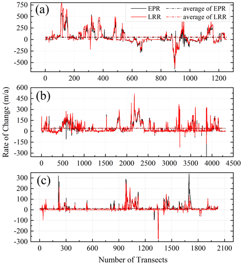
The shoreline change rates in the three economically developed coastal areas from 1990 to 2019 are shown in Figs. 8 and 9. The shoreline generally shows an expanding trend towards the seaside but with spatially distinct characteristics. The change rate of the shoreline of BHB-YREZ was faster than those of YRE-HZBZ and PREZ followed by that of YRE-HZBZ. In BHB-YREZ, the average EPR and LRR were 43.59 and 57.40 km yr⁻¹ from 1990 to 2019, respectively. The maximum EPR and LRR were 576.95 m yr⁻¹ and 781.59 km yr⁻¹, respectively, and the minimum EPR and LRR were −646.42 and −554.34 km yr⁻¹, respectively. In the YRE-HZBZ, the average EPR and LRR of the shoreline were 39.1 and 43.85 km yr⁻¹ from 1990 to 2019, respectively. The maximum EPR and LRR were 471.66 m yr⁻¹ and 424.50 km yr⁻¹, respectively, and the maximum EPR and LRR were −345.05 and −175.62 km yr⁻¹. In the PREZ, the average EPR and LRR of the shoreline were 13.42 and 10.11 km yr⁻¹ from 1990 to 2019, respectively. The maximum EPR and LRR were 339.92 m yr⁻¹ and 136.85 km yr⁻¹, respectively, and the maximum EPR and LRR were −249.47 and −270.57 km yr⁻¹.

Figure 8 Change rate of shorelines over BHB-YREZ (a), YRE-HZBZ (b), and PREZ (c) from 1990 to 2019.

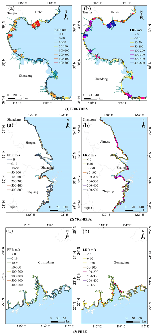
Figure 9 Map of the shoreline change rate in three regions from 1990 to 2019: (1) BHB-YREZ, (2) YRE-HZBZ, (3) PREZ. (a) EPR, (b) LRR.

Since 1990, more than 79.4 % of China's shorelines have conspicuously demonstrated a significant positive trend of coastal change (Table 4), with a notable contrast between accretion and erosion dynamics (20.6 % erosion). Regionally, the PREZ region, on the whole, maintains relative stability, with only 9.9 % of shorelines exhibiting temporal trends of alteration (Table 4 and Fig. 9). The most dynamic coastal regions were BHB-YREZ and YRE-HZBZ, where over 19.7 % and 31.4 % of shorelines exhibited significant trends of coastal change dominated by accretion and erosion, respectively.

Table 4 Erosion and accretion areas in stages from 1990 to 2019 (in km²).

5 Discussion

5.1 Caveats and limitations of consistency test

This study employs remote-sensing-based coastal change results to validate against other remote-sensing-based shoreline datasets. The GSV and Coastline_ECS datasets share similarities in data sources (Landsat imagery) and processing methodologies with the approach used in this research, and the mean absolute deviation is less than 2 px (60 m), indicating a certain level of consistency between the results and other shoreline datasets. However, the limitation of this validation approach lies in the fact that consistency does not necessarily equate to actual accuracy, particularly if the datasets themselves contain errors (Vos et al., 2019b). Such consistency-based validation may lead to an overestimation of data accuracy (Wulder et al., 2018). Therefore, while the results in this study exhibit good consistency in the validation tests, their actual accuracy still requires further verification.

Field measurement data (e.g., beach surveys and on-site investigations) serve as independent validation sources and can more accurately assess the reliability of the extracted results (Pardo-Pascual et al., 2012; Vos et al., 2019a), providing a more comprehensive and objective validation framework. However, access to such field measurement data is limited due to confidentiality.

Additionally, it is important to acknowledge the potential limitations of using modeled data for mutual validation. The inherent uncertainties in different models, the errors involved, and the systematic biases (Vos et al., 2019b) that may exist across various coastal environments and remote sensing datasets could all affect the reliability of the validation results. Therefore, in future research, we aim to explore the applicability and limitations of such model validation approaches, providing insights into the matter and suggestions for further improvements.

5.2 Forces driving shoreline change

5.2.1 Natural factors

Natural factors that affect shoreline changes mainly include geomorphic features, climate change (Qin et al., 2023), tidal waves, sediments, sea level rise, and other natural environments. Geological structures and topography of the coastal zone determine shoreline stability (Dillenburg et al., 2000). Rocky shorelines are usually located at the base of cliffs or bluffs and are more stable compared to sandy, muddy, and biological shorelines that are distributed on shallow beaches and flatlands (Zhang et al., 2021). Artificial shorelines developed and constructed based on natural shorelines are also less susceptible to natural environmental influences. Sandy, muddy, and biological shorelines are more sensitive to tidal waves, sediments, and sea level rise. Sediment transport is generated by water, wind, and gravity, and its erosion and deposition processes can impact the evolution of estuarine morphology (Chaudhry, 2008), resulting in coastal accretion or erosion. BHB-YREZ, YRE-HZBZ, and PREZ are in the estuarine deltas of major rivers with the largest shoreline changes. Sediment is an important factor leading to coastal accretion or erosion (Luan et al., 2021), and it affects the process of continental margin formation.

The sediments in BHB-YREZ, YRE-HZBZ, and PREZ primarily originate from Yellow River, Yangtze River, and Pearl River. To analyze the impacts of sediment transport on shoreline variations, we collected sediment data (http://www.mwr.gov.cn/sj/, last access: 12 November 2024) of the Yellow River and the Yangtze River from the Lijin station and the Datong station from 2000 to 2019, respectively, and from the main stream of the Pearl River from the Gaoyao station, the Shijiao station, and the Boluo station from 2001 to 2019, respectively (Fig. 10). Here, the hydrological data of the Pearl River estuary are the sum of the data from the three hydrological stations.

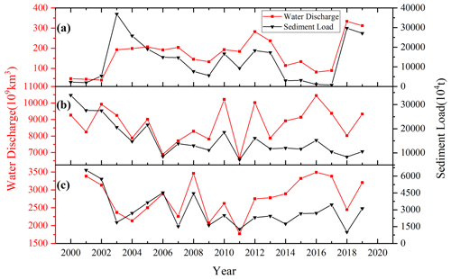
Figure 10 Annual water discharge and annual sediment load. (a) Lijin Hydrometric Station from 2000 to 2019; (b) Datong Hydrometric Station from 2000 to 2019; (c) Gaoyao, Shijiao, and Boluo Hydrometric Stations from 2001 to 2019.

Figure 10 shows that sediment transport in the Yellow River estuary reached its peak in 2003. Afterward, it began a decreasing trend, reaching a minimum in 2017. The sediment transport in the Yangtze River estuary was the highest in 2000. Following that, it began to decline in a fluctuating manner from 2000. The sediment transport in the Pearl River estuary was highest in 2001 and exhibited a general decreasing trend. A similar trend can be observed between water discharge and sediment load.

In Fig. 10a, we observe a similarity in the trends between discharge and load. According to the official Yellow River Sediment Bulletin (http://www.mwr.gov.cn/sj/, last access: 12 November 2024), several large-scale hydraulic projects were implemented between 2002 and 2010. Starting from 2003, the total amount of sediment load had not increased significantly, which consequently led to the corresponding decrease in the shoreline length in the estuarine region. In Fig. 10b, sediment transport from the Yangtze estuary declined sharply in the 5 years following the construction of the Three Gorges Dam in 2002 (Yang et al., 2015; Luan et al., 2021). In Fig. 10c, the construction of the Longtan Water Conservancy Project on the Pearl River started in 2001, resulting in a large reduction in the sediment carried by the Pearl River into the sea. When combined with Fig. 7b, it becomes evident that the river sediment transport is related to changes in coastal areas. In the four periods after 2000, the change in the area of the PREZ decreased significantly and tended to stabilize compared to the period from 1995 to 2000.

5.2.2 Anthropogenic factors

In recent decades, the spatio-temporal changes in the shoreline have been constrained by external environmental conditions, i.e., mainly the influence of geographical location, policies, and socio-economic factors. River deltas with flat topography and favorable location conditions are the main zones of population concentration and socio-economic development. Coastal development activities gravitate around these areas and extend outwards. The three major coastal economic areas, BHB-YREZ, YRE-HZBZ, and PREZ, are the most developed regions in China, which are also experiencing the most pronounced shoreline changes. Examining the location and area changes in shorelines in the three coastal economic zones, human activities, such as land reclamation, emerge as the main driving factors affecting shoreline changes (Cai et al., 2022).

During the 1990s, when China was in the early stages of developing the socialist market economy, the demand for high-quality seafood for domestic consumption and export to overseas markets increased significantly, prompting a rapid expansion of the mariculture industry (Wang et al., 2014). As a result, large areas of coastal tidal flats were reclaimed for the purposes of aquaculture. After 2000, large-scale land reclamation took place to accommodate the rapid development of China's coastal economy (Fig. 11).

Figure 11 (a) Reclamation in China from 2002 to 2015. (b) Length of main coastal ports above the designated size from 1990 to 2019.

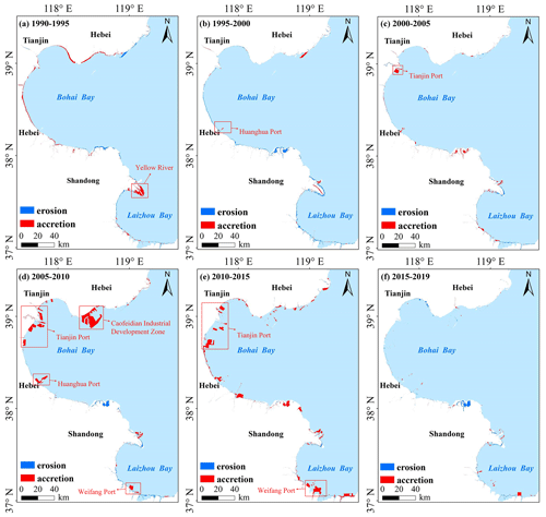
In BHB-YREZ, the area with the greatest changes along the shoreline was concentrated in the northern part of Bohai Bay, including parts of Caofeidian, Tianjin, and Dongying. To align with the national energy and transportation development strategy, optimize the heavy chemical industry in the northern region, and accelerate the economic integration development of the Bohai Sea region, Caofeidian was included in the national 11th Five-Year Plan and the first batch of circular economy demonstration parks. Development was officially approved by the General Plan for the Industrial Development of Caofeidian Circular Economy Demonstration Zone. In 2005, the construction of the Caofeidian Industrial Development Zone (Fig. 12d) began, with a total area of 310 km² to be reclaimed, making it the largest land reclamation project in China. In 2002, Tianjin Port (Fig. 12c) started the Beida breakwater project and the reclamation project of the Dongjiang Bonded Port Area. The east and south outer dikes of the north breakwater were closed, and the construction of the port area began with mud-blowing and reclamation. In 2011, the Ministry of Transport and the Tianjin Municipal People's Government approved the Master Plan of Tianjin Port (2011–2030) (http://jtys.tj.gov.cn/, last access: 12 November 2024) (Fig. 12e). By 2019, the layout of “one port and eight districts”, as determined in the plan, was formed, including the ports of Beijiang, Dongjiang, Nanjiang, Gaoshaling, Dagang, Beitang, and Haihe. In 1997, construction of the Port of Huanghua (Fig. 12b) in Hebei Province began. In 2008 (https://www.ufsoo.com/port/huanghua/, last access: 12 November 2024), the Ministry of Transport and the People's Government of Hebei Province approved the Master Plan of Huanghua Port, with a plan to build four major ports: a coal port, a comprehensive port, a bulk cargo port, and an estuary port. In 2005, Weifang started to build a 10 000 t wharf and a 10 000 t waterway along with a wave barrier dike project (https://www.ufsoo.com/port/weifang/, last access: 12 November 2024). According to the Master Plan of Weifang Port approved by the Shandong Provincial People's Government, the Weifang Port central port area was built into a harbor area surrounded by double dikes and a single entrance in 2010.

Figure 12 Area and locations of land erosion and accretion in BHB-YREZ.

The coastal changes in the Yellow River estuary region are mainly caused by the deposition of suspended river particles (Fig. 12a), resulting in a dynamic alteration process of its shoreline. From 1996 to 2003, the original channel area of the Yellow River estuary was reduced, and the new channel gradually expanded toward the sea, leading to a reduction in the change rate in the south of the Yellow River estuary. Between 2003 and 2013, the new river channel further expanded seaward, causing the Yellow River estuary to bifurcate on both sides of the river, and the newly expanded area exhibited more rapid changes (Peng et al., 2010; Zhu et al., 2021).

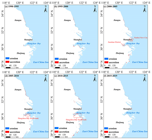
In YRE-HZBZ, the majority of shoreline changes were concentrated in the eastern part of Shanghai and the southern part of Hangzhou Bay. In 2002, Nanhui New City (Fig. 13c) in Shanghai was developed and constructed, and the land was reclaimed for urban residential areas and coastal industrial development. To meet the development needs of the Hangzhou Bay greater bay area and Shanghai–Hangzhou integration, Jianshan District (Fig. 13c) was developed and constructed in 2005, with an artificially reclaimed area of about 42 km², mainly for aquaculture areas and urban construction. Cultivation, farming land, and urban construction are the primary driving forces of shoreline changes along the south coast of Hangzhou Bay. From 2002 to 2011, numerous reclamation projects were carried out on the south coast of Hangzhou Bay (Fig. 13d–e) to promote the continuous expansion of the shoreline toward the ocean side. In 2019, Zhejiang Province formulated the Implementation Plan of Zhejiang Province for Strengthening Protection of Coastal Wetlands and Strictly Controlling Reclamation (Department of Natural Resources of Zhejiang Province, 2019) based on the Notice on Strengthening Protection of Coastal Wetlands and Strictly Controlling Reclamation issued by The State Council and the Notice of the Ministry of Natural Resources on Further Clarifying the Handling of Historical Issues Left Over from Reclamation. This plan proposes the control of the reclamation process.

Figure 13 Area and locations of land erosion and accretion in YRE-HZBZ.

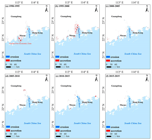
In PREZ, the primary focus of land reclamation at the Pearl River estuary is to generate greater economic and social benefits through the construction of ports, airports, and other infrastructure (Hu and Wang, 2022). The construction of Shenzhen Airport (Fig. 14) was completed in 1990. In 2012, the port of Shenzhen successively completed 10 port areas, including Shekou, Chiwan, and Yantian. On the western bank of the Pearl River estuary, land reclamation has been mainly dedicated to port construction. The Port of Guangzhou is expanding to meet the needs of economic development. By 2019, four major port areas (Fig. 14b) were planned to be developed – Inner Harbor, Huangpu, Xinsha, and Nansha. Meanwhile, on the farther western side of the Pearl River Estuary, extensive shoreline expansion was mainly earmarked for urban construction, such as the Gaolan Port Economic Development Zone (Fig. 14a). With the implementation of the “Outline of the Plan for the Reform and Development of the Pearl River Delta (2008–2020)”, Gaolan Port has resulted in the acceleration of the urbanization process on the western bank of the Pearl River estuary (Hong Kong And Macao Office Of The State Council, 2009).

Figure 14 Area and locations of land erosion and accretion in PREZ.

5.2.3 Shoreline length

Shoreline length is widely recognized as a challenging and potentially problematic metric for analyzing coastal change over time. The primary issue stems from the “coastline paradox” (Mandelbrot, 1967), which highlights the scale dependency of shoreline measurements. Due to the fractal geometry of coastlines, the measured length can vary depending on image resolution or spatial scale. Additionally, shoreline length is highly susceptible to noise (Vos et al., 2019a), which can be influenced by temporal variations and differences between satellite sensors, such as those between Landsat 5 and Landsat 8.

To address the inherent noise and variability introduced by different satellite sensors, we applied the HANTS algorithm to smooth the time series data and reduce the impact of short-term fluctuations and sensor-specific inconsistencies (Zhu and Woodcock, 2014; Lhermitte et al., 2011). This method effectively filters out much of the random noise, enabling a more consistent and robust comparison of shoreline length over time. Furthermore, by focusing on regional-scale shoreline trends rather than small-scale local variations (Schuerch et al., 2018), the analysis mitigates the sensitivity to the scale dependency emphasized by the coastline paradox (Mentaschi et al., 2018).

While we acknowledge that shoreline length may not be an ideal metric in all contexts, we argue that the methodological steps taken – particularly the use of the HANTS algorithm and the emphasis on large-scale trends – significantly reduce the uncertainties associated with this metric. Nevertheless, it is important to consider these limitations when interpreting the results, and we have carefully documented the potential pitfalls in this regard. Future studies could benefit from exploring additional metrics, such as shoreline position or area change (Fogarin et al., 2023), to complement the findings presented here.

5.3 Uncertainty analysis of shoreline extraction

To investigate the influence of image resolution on coastal line mapping, a study was conducted in the BHB-YREZ, YRE-HZBZ, and PREZ regions using input images of varying resolutions. A comparative analysis was performed between shorelines derived from Landsat 8 (L8) and Sentinel-2 (S2) data acquired in 2019 and manually digitized shorelines based on Google Earth imagery. The outcomes are illustrated in Fig. 15.

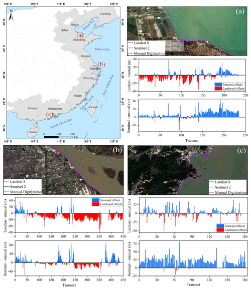
Figure 15 Comparison between the L8, S2, and corresponding results of manual digitization. Panels (a), (b), and (c) are the difference between L8, S2, and manual digitization. ME and MAE are mean error and mean absolute error, respectively. The images in panels (a), (b), and (c) are true-color composite images of S2.

Transects were established along the shorelines at regular intervals of 500 m, facilitating a distance-based comparison between the shorelines derived from L8, S2, and the manually digitized shorelines. In the L8, all three regions exhibited greater landward offsets (red bars) as compared to seaward offsets. The respective mean error (ME) was −8.5, −18.15, and −9.41 m. Conversely, in S2, the shorelines in the BHB-YREZ and PREZ regions displayed larger seaward offsets (blue bars in Fig. 15), while the YRE-HZBZ region showed greater landward offsets. In the BHB-YREZ region, the mean absolute error (MAE) for L8 and S2 was 5.29 and 8.72 m, respectively, with L8 exhibiting superior performance and an MAE difference of 3.43 m. In the YRE-HZBZ region, the average absolute deviations for L8 and S2 was 12.45 and 11.37 m, respectively, with S2 marginally outperforming L8, exhibiting a mere 1.02 m difference in MAE. In the PREZ region, the MAE for L8 and S2 were 6.99 and 18.70 m, respectively, with L8 performing better with an MAE difference of 11.71 m. Based on the comparative analysis of L8 and S2 performance in shoreline extraction, it was observed the spatial resolution of the images was not the decisive factor impacting the extraction results. In the majority of cases, Sentinel-2 did not demonstrate superior extraction outcomes.

5.4 Advantages and limitations of the proposed method and dataset

This study introduced a threshold segmentation method based on MNDWI time series reconstruction to generate a dataset of China's shoreline using a time series of Landsat images on the GEE platform. This represents the first interannual dataset of China's shoreline at a 30 m spatial resolution from 1990 to 2019. The successful implementation of this study is attributed to the availability of open-access satellite data, a simple but robust shoreline extraction method, and the powerful computational capabilities of the GEE platform.

Firstly, the open access and free availability of land satellite imagery provided an opportunity to obtain high-frequency and high-quality observational data. The dense time series of Landsat images enables monitoring of surface changes through remote sensing. The Landsat series provides observations within a 16 d repeat cycle over several decades. The observation frequency (Yao et al., 2019) formed the basis for generating reliable shoreline data as the monitoring task is based on the assumption of image availability near the highest tidal levels. By utilizing all available Landsat images, we increased the quality of observations and obtained better information on China's coastal zone.

Secondly, rather than using a simple composite image approach to synthesize the median reflectance values of all image pixels during the target period, we applied the HANTS method to reconstruct the images. While using a median composite image (Bishop-Taylor et al., 2021) minimizes the interference of cloud contamination with surface features, it also alters the original pixel values, resulting in the loss of detailed information and an inaccurate representation of the original tidal state. Instead, the HANTS method preserves the integrity of the original pixel values by fitting only the pixels that experience image gaps due to cloud masking while leaving other high-quality pixels unchanged. The Otsu threshold segmentation algorithm, being fully automated and requiring no manual intervention or training samples, automatically determines the threshold value. The threshold segmentation method based on exponential time series reconstruction effectively suppressed non-water surfaces and obtained accurate water extent information.

Thirdly, the utilization of the GEE platform allowed us to rapidly access tens of thousands of Landsat images and perform parallel processing, thereby improving the efficiency of the experiments. Additionally, GEE synchronizes all Landsat data and provides processed products at different levels, including top-of-atmosphere and surface reflectance data.

However, it is important to note that applying this method in tropical regions may introduce noticeable errors due to the higher frequency of cloud cover. To overcome this limitation and track long-term shoreline dynamics in these regions, it is recommended to incorporate Sentinel-1 synthetic-aperture radar (SAR) images (Dike et al., 2024). The classification of shoreline types enhances the understanding of their formation mechanisms, evolutionary processes, and interactions with environmental factors. It also facilitates the evaluation of the impacts of human activities and natural processes on shorelines. Consequently, future research can employ the shoreline dataset generated in this study in conjunction with shoreline type classification.

In this study, we selected 17 tide stations with extensive tidal flat coverage and used satellite images captured during high-tide periods (Jia et al., 2021). While this approach effectively captures key shoreline characteristics in areas with significant tidal coverage, the limited distribution of tide stations means that the results may not fully represent tidal conditions across the entire study area, particularly in regions with complex tidal dynamics or varying intertidal slope gradients. Using high-tide imagery helps to reduce the direct impact of tidal fluctuations on shoreline extraction (Mao et al., 2021); however, variations in tide levels across different locations could still introduce systematic biases. And in reality, we cannot guarantee that the satellite's transit time will be exactly at the peak moment. Therefore, our shoreline results differ from the maximum or average high-tide line as the coastline, which only represents the water edge line close to the high-tide level from remote sensing images. This dataset already meets the needs of analyzing the change trends and characteristics of large-scale regions while avoiding the sensitivity of standard coastlines as confidential data.

6 Data availability

China's mainland shorelines over 30 years can be accessed at https://doi.org/10.57760/sciencedb.16228 (Yang et al., 2024). This dataset is licensed under a CC-BY 4.0 license.

7 Conclusions

This research produced the first 30-year spatio-temporal change analysis of China's mainland shoreline based on the time series data of Landsat images from 1990 to 2019. The high frequency of data acquisition used in this study enabled a detailed analysis of shoreline changes in mainland China over the past 30 years. The shorelines in different periods were quantitatively analyzed using several evaluation indicators, such as shoreline length and area changes, linear regression rate, and end point rate. In addition, the influence of tidal correction on the accuracy of shoreline extraction and the natural and anthropogenic drivers of shoreline change in BHB-YREZ, YRE-HZBZ, and PREZ were also explored.

The results demonstrated that although the spatio-temporal shoreline changes in mainland China are complicated. While both accretion and erosion were observed, accretion was the dominant pattern of shoreline change in mainland China over the past 30 years, especially in BHB-YREZ, YRE-HZBZ, and PREZ. Throughout the entire study period, the length of China's mainland shoreline increased by 485.78 km. The shoreline change increased the land area by 7088.25 km². Compared with natural factors, anthropogenic activities such as land reclamation were the major drivers of all shoreline changes.

Since the 1990s, shoreline types have changed rapidly. There were large differences in the change patterns of different types of shorelines. In the future, we can classify shoreline types based on the shorelines extracted in this study. This will improve our ability to understand the degree of shoreline utilization and explore the influence of natural and anthropogenic factors on different types of shoreline changes. The outcomes of this research provide support for more effective restoration, compensation of damaged coastal ecosystems, and sustainable development of coastal resources.