the Creative Commons Attribution 4.0 License.
the Creative Commons Attribution 4.0 License.
 | 22 Jan 2024
CoCO2-MOSAIC 1.0: a global mosaic of regional, gridded, fossil, and biofuel CO2 emission inventories
Ruben Urraca
Greet Janssens-Maenhout
Nicolás Álamos
Lucas Berna-Peña
Monica Crippa
Sabine Darras
Stijn Dellaert
Hugo Denier van der Gon
Mark Dowell
Nadine Gobron
Claire Granier
Giacomo Grassi
Marc Guevara
Diego Guizzardi
Kevin Gurney
Nicolás Huneeus
Sekou Keita
Jeroen Kuenen
Ana Lopez-Noreña
Enrique Puliafito
Geoffrey Roest
Simone Rossi
Antonin Soulie
Antoon Visschedijk
Gridded bottom-up inventories of CO2 emissions are needed in global CO2 inversion schemes as priors to initialize transport models and as a complement to top-down estimates to identify the anthropogenic sources. Global inversions require gridded datasets almost in near-real time that are spatially and methodologically consistent at a global scale. This may result in a loss of more detailed information that can be assessed by using regional inventories because they are built with a greater level of detail including country-specific information and finer resolution data. With this aim, a global mosaic of regional, gridded CO2 emission inventories, hereafter referred to as CoCO2-MOSAIC 1.0, has been built in the framework of the CoCO2 project.
CoCO2-MOSAIC 1.0 provides gridded (0.1∘ × 0.1∘) monthly emissions fluxes of CO2 fossil fuel (CO2ff, long cycle) and CO2 biofuel (CO2bf, short cycle) for the years 2015–2018 disaggregated in seven sectors. The regional inventories integrated are CAMS-REG-GHG 5.1 (Europe), DACCIWA 2.0 (Africa), GEAA-AEI 3.0 (Argentina), INEMA 1.0 (Chile), REAS 3.2.1 (East, Southeast, and South Asia), and VULCAN 3.0 (USA). EDGAR 6.0, CAMS-GLOB-SHIP 3.1 and CAMS-GLOB-TEMPO 3.1 are used for gap-filling. CoCO2-MOSAIC 1.0 can be recommended as a global baseline emission inventory for 2015 which is regionally accepted as a reference, and as such we use the mosaic to inter-compare the most widely used global emission inventories: CAMS-GLOB-ANT 5.3, EDGAR 6.0, ODIAC v2020b, and CEDS v2020_04_24. CoCO2-MOSAIC 1.0 has the highest CO2ff (36.7 Gt) and CO2bf (5.9 Gt) emissions globally, particularly in the USA and Africa. Regional emissions generally have a higher seasonality representing better the local monthly profiles and are generally distributed over a higher number of pixels, due to the more detailed information available. All super-emitting pixels from regional inventories contain a power station (CoCO2 database), whereas several super-emitters from global inventories are likely incorrectly geolocated, which is likely because regional inventories provide large energy emitters as point sources including regional information on power plant locations. CoCO2-MOSAIC 1.0 is freely available at zenodo (https://doi.org/10.5281/zenodo.7092358; Urraca et al., 2023) and at the JRC Data Catalogue (https://data.jrc.ec.europa.eu/dataset/6c8f9148-ce09-4dca-a4d5-422fb3682389, last access: 15 May 2023; Urraca Valle et al., 2023).
- Article
(3242 KB) - Full-text XML
-
Supplement
(2464 KB) - BibTeX
- EndNote


The European Commission (EC), together with the European Centre for Medium-Range Weather Forecasts (ECMWF), the European Space Agency (ESA), and the European Organisation for the Exploitation of Meteorological Satellites (EUMETSAT), are developing the Copernicus CO2 Monitoring and Verification Support (CO2MVS) capacity, a new operational service to monitor and verify anthropogenic CO2 emissions with observation-based evidence supporting policymakers (Janssens-Maenhout et al., 2020; Pinty et al., 2017). CO2MVS will exploit the unprecedented observations from the upcoming Copernicus CO2 mission (CO2M) (Sierk et al., 2021), which initially foresees the launch of two or three polar-orbiting satellites that will sample XCO2, XCH4, and NO2 at around 2–4 km2 and with an accuracy better than 0.7 ppm (Meijer et al., 2020). The CO2MVS system will combine satellite and in situ measurements with prior information using an advanced data assimilation scheme (Ciais et al., 2015; Pinty et al., 2017, 2019). The initial design of this system is being supported by the H2020-funded CoCO2 project (https://coco2-project.eu/; last access: 1 April 2023), which will develop a pre-operational prototype of the CO2MVS continuing the efforts started by CHE (https://www.che-project.eu/; last access: 1 April 2023) and VERIFY (https://verify.lsce.ipsl.fr/; last access: 1 April 2023) projects.
The main challenges faced by CO2MVS in particular, and by CO2 inversions in general, are that satellites measure column concentrations, rather than emissions, and that the signal of anthropogenic fossil emissions in atmospheric concentrations is small (and with much smaller variation) relative to the oscillating signal of natural fluxes between the land and ocean surfaces and the atmosphere. Bottom-up gridded emission inventories are a key component to address these challenges (Ciais et al., 2015; Pinty et al., 2017). They supply essential prior information to initialize transport models reducing the uncertainty of top-down inversions. They are also complementary to the top-down estimates and provide traceability to the primary activity data. Despite the advances done in source attribution using co-emitters, high-resolution images, or radiocarbon, bottom-up inventories can identify with a much higher level of detail the exact source of anthropogenic emissions.
During the past decade, several efforts have been made to produce anthropogenic bottom-up inventories of CO2 emissions. The most prominent examples at the global scale are the Emissions Database for Global Atmospheric Research (EDGAR) (Janssens-Maenhout et al., 2019; Crippa et al., 2021; https://edgar.jrc.ec.europa.eu/dataset_ghg60; last access: 1 April 2023), the Copernicus Atmosphere Monitoring Service global anthropogenic emissions (CAMS-GLOB-ANT) (Soulie et al., 2023), the Open-source Data Inventory for Anthropogenic CO2 (ODIAC) (Oda et al., 2018), the Community Emissions Data System (CEDS) (Hoesly et al., 2018; McDuffie et al., 2020), the Global Carbon Grid (GID) (http://gidmodel.org; last access: 1 April 2023), and the near-real-time Global Gridded Daily CO2 Emission Dataset (GRACED) (Dou et al., 2022). Gridded inventories used for operational global scale inversions need to meet some requirements that may lead to a loss of information. First, they need to provide near-real-time emissions, whereas most of the previous efforts are based on information that typically becomes available with a lag of at least 2 years (Ciais et al., 2015). The exceptions are EDGAR, which provides near-real-time data using a fast-track approach based on BP statistics, and GRACED, which uses national Carbon Monitor data produced from hourly and daily electrical consumption and production data and daily mobility indices, among others (Liu et al., 2020a, b). Second, gridded inventories should provide spatially and methodologically consistent emissions for global inversion models. This may lead to the exclusion of more detailed information available in some regions because spatial inconsistencies in the border between two inventories (e.g., spatial discontinuities in road or aviation emissions) would have a negative impact on the inversion model.
Regional inventories can be used to measure this loss of information due to the uptake of local data at much finer spatial resolution and the inclusion of country-specific activity and emissions information. Some examples are CAMS regional inventory for greenhouse gases (CAMS-REG-GHG) over Europe (Kuenen et al., 2022), the Dynamics-Aerosol-Chemistry-Cloud Interactions in West Africa (DACCIWA) dataset over Africa (Keita et al., 2021), the Multi-Resolution Emission Inventory for China (MEIC) (Li et al., 2017; Zheng et al., 2018), the Inventario Nacional de Emisiones Antropogenicas (INEMA) for Chile (Álamos et al., 2022), the Argentina Emission Inventory produced by the Research Group on Atmospheric and Environmental Studies (GEAA-AEI) (Puliafito et al., 2021), the Regional Emission Inventory in Asia (REAS) (Kurokawa and Ohara, 2020), or the VULCAN dataset over the USA (Gurney et al., 2020).
With this context and the previously stated requirements, in the framework of the CoCO2 project, a comprehensive global mosaic of gridded, regional CO2 emission inventories that are primarily official reference data or widely used in each region or country has been built. This dataset will be hereafter referred to as the CoCO2-MOSAIC 1.0. Compared with the global inventories, CoCO2-MOSAIC 1.0 includes all the regional information available, without the limitation of providing spatially and methodologically consistent emissions. Besides, the mosaic does not aim to provide near-real-time estimations, which allows us to include regional information that becomes available with some years of delay. Therefore, it could be considered a regionally accepted reference, and as such, it could be used to assess the quality of the global inventories used in global inversions. CoCO2-MOSAIC 1.0 could be also used to run regional atmospheric inversions within the spatial domain of each regional inventory. This would be consistent with how the Hemispheric Transport of Air Pollution (HTAP) mosaic (Janssens-Maenhout et al., 2015; Crippa et al., 2023, https://edgar.jrc.ec.europa.eu/dataset_htap_v3; last access: 1 April 2023) has been extensively used by air pollutant models. It is noteworthy that the use of regional emission datasets for assessing global inventories is currently limited by their accessibility (e.g., different spatial resolution, sector description, or data format). CoCO2-MOSAIC 1.0 solves this issue by providing harmonized access to regional datasets at a global scale, helping users to replicate inter-comparisons such as the one conducted in this study.
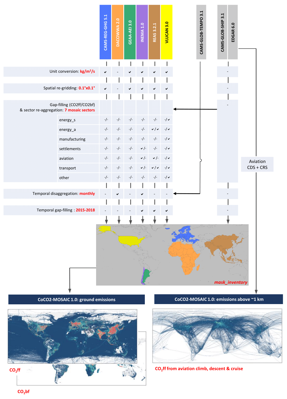
Figure 1Flowchart of the CoCO2-MOSAIC 1.0 methodology. CDS: climbing and descent; CRS: cruise. The checkmark means that the specific processing step was applied to the inventory. Gap-filling was done independently for CO2ff and CO2bf. Sectors may have been gap-filled fully or partially (see Supplement).
CoCO2-MOSAIC 1.0 provides gridded (0.1∘ × 0.1∘) monthly emissions fluxes from CO2 from fossil fuel (CO2ff, long cycle) and CO2 from biofuel (CO2bf, short cycle) from 2015 to 2018. The regional inventories integrated are CAMS-REG-GHG 5.1, DACCIWA 2.0, GEAA-AEI 3.0, INEMA 1.0, REAS 3.2.1, and VULCAN 3.0. EDGAR 6.0 and CAMS-GLOB-SHIP 3.1 are used for gap-filling, whereas CAMS-GLOB-TEMPO 3.1 is used for temporal disaggregation. The paper describes the methodology used to build CoCO2-MOSAIC 1.0 and benchmarks some of the most widely used global inventories against CoCO2-MOSAIC 1.0: CAMS-GLOB-ANT 5.3, EDGAR 6.0, ODIAC 2021b, and CEDS v2020_04_21. The inter-comparison is made using 2015 data, analyzing their total and per-sector emissions in each region, their spatial and temporal weight factors, and the location and magnitude of super-emitting pixels, among other aspects.
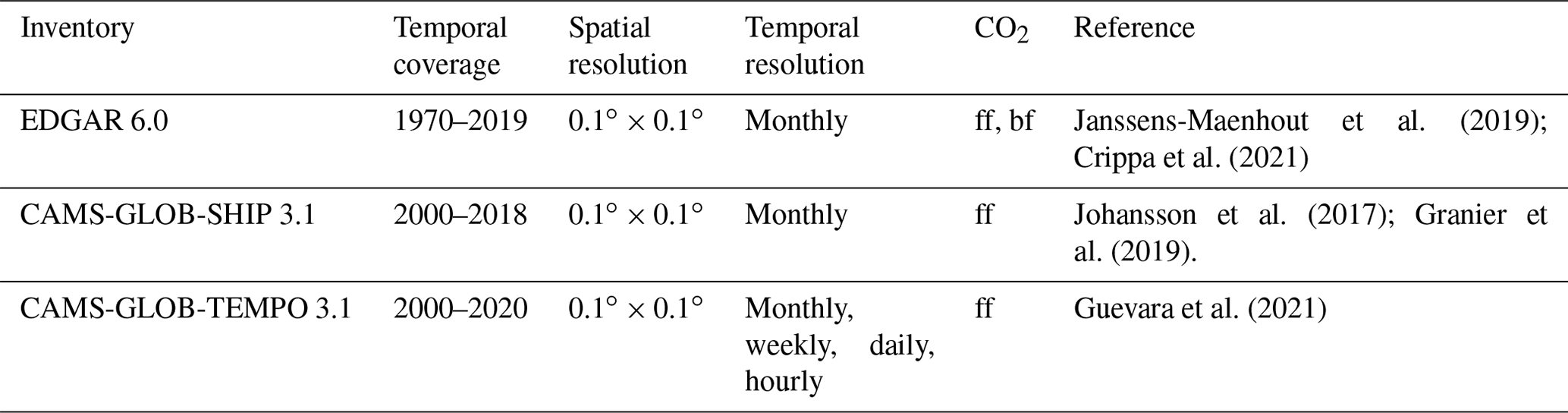
2.1 Input emission inventories
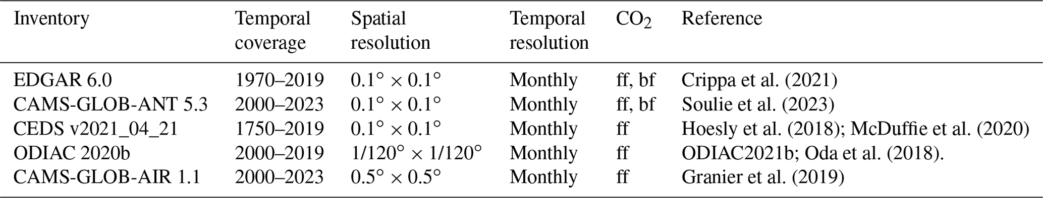
The regional inventories integrated by CoCO2-MOSAIC 1.0 are summarized in Table 1. Global inventories are used to gap-fill missing or incomplete sectors, and countries without regional information (Table 2). The default global inventory for gap-filling is EDGAR 6.0, replacing EDGAR 6.0 shipping emissions (TRO_Ship) by CAMS-GLOB-SHIP 3.1. CAMS-GLOB-TEMPO 3.1 monthly profiles are used to disaggregate temporally the emissions of inventories only providing annual estimates. All the global inventories are from CAMS except EDGAR, which was used instead of CAMS-GLOB-ANT because a high sectoral disaggregation was needed for gap-filling. A complete description of each inventory methodology and their sector definitions is available in the Supplement.
Table 1Description of the regional emission inventories integrated by CoCO2-MOSAIC 1.0.
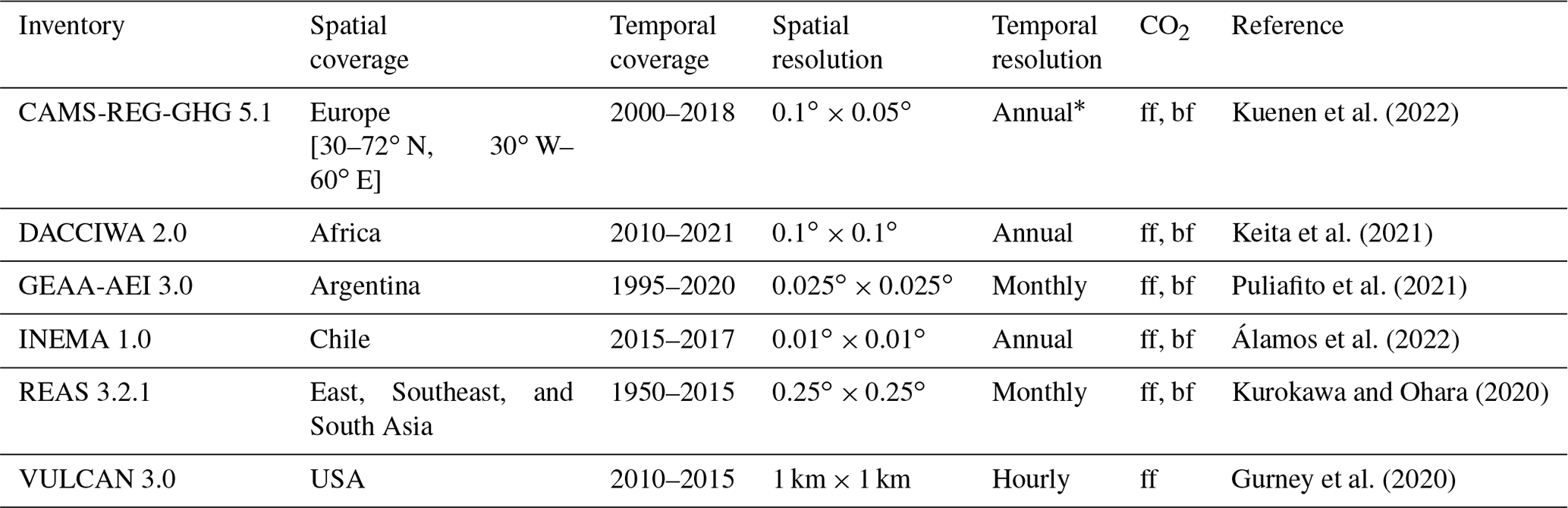
∗ Monthly emissions in CAMS-REG-GHG were calculated using the default temporal profiles provided with the dataset.
Table 2Description of the global datasets used to gap-fill CoCO2-MOSAIC 1.0.
2.2 Methodology
This section describes the main steps followed to build CoCO2-MOSAIC 1.0. A general overview of the methodology is provided in Fig. 1.
2.2.1 Unit conversion
Regional inventories providing emissions in kilograms per year were converted into kilograms per square meter per second using the cell area included as CoCO2-MOSAIC 1.0 auxiliary layer. VULCAN 3.0 emissions were transformed from kg C to kg CO2 using the atomic mass of C in CO2 ().
2.2.2 Spatial re-gridding
CoCO2-MOSAIC 1.0 uses a 0.1∘ × 0.1∘ grid with the upper-left corner of the upper-left pixel at [−180.0∘, −90.0∘]. All regional inventories except DACCIWA 2.0 had to be re-gridded. CAMS-REG-GHG 5.1 (0.1∘ × 0.05∘), GEEA-AEI 3.0 (0.025∘ × 0.025∘), and INEMA 1.0 (0.01∘ × 0.01∘) grids were perfectly aligned with the mosaic grid and proportional to it, so the raw emissions inside each mosaic pixel were directly averaged. GEAA-AEI point emissions were averaged over the 0.1∘ × 0.1∘ pixel containing the point source. VULCAN 3.0 point, line, and polygon emissions were directly aggregated into the mosaic grid to minimize re-gridding errors. REAS 3.2.1 (0.25∘ × 0.25∘) emissions were first downscaled from to a 0.05∘ × 0.05∘ grid by just replicating the emission fluxes. At coastal pixels, emission fluxes were re-calculated assuming that emissions over the 0.05∘ × 0.05∘ sea pixels were zero. (REAS does not include shipping emissions.) Then, 0.05∘ × 0.05∘ emission fluxes were averaged into the mosaic grid. REAS power plant emissions are available as point sources, and they were averaged over the 0.1∘ × 0.1∘ pixel containing the power plant.
2.2.3 Gap-filling missing emissions and sector aggregation
CoCO2-MOSAIC 1.0 provides CO2ff and CO2bf emissions in seven groups of sectors: energy_s (super-emitting sources above kg m−2 s−1), energy_a (average emitters), manufacturing, settlements, transport, aviation (land and take-off (LTO)), and “other”. These sectors were defined by grouping EDGAR 6.0 categories as shown in Table 3. The choice of a super-emitters threshold of kg m−2 s−1 was made in Choulga et al. (2021) to filter a reasonable number of super-emitting pixels whose accuracy could be manually checked to reduce the uncertainty of energy emissions. Note that, for simplicity, solid waste incineration includes both incineration with and without energy recovery due to the high uncertainty of separating these two groups. This choice was made at the CHE project (Choulga et al., 2021) and was kept in CoCO2 for consistency.
Table 3 also describes how the emissions by sector from regional inventories were aggregated into the mosaic sectors. If the emissions of a sector in a region were fully or partly missing, they were gap-filled with the default global inventory (EDGAR 6.0 + CAMS-GLOB-SHIP 3.1). We only gap-filled a missing category/component if its contribution to the mosaic sector was above 1 % (based on EDGAR 6.0) (Table S8 in the Supplement). The sector “other” was not gap-filled to avoid a potential double counting of the emissions, because these emissions could be partly included in other sectors. In any case, the emissions of this sector are expected to be low compared with the others. The mosaic follows the definition of biofuels provided by the International Energy Agency (IEA) (see Supplement). CO2ff and CO2bf emissions were defined by each regional inventory and we verified the consistency of regional methodologies with the IEA definition. Note that agricultural waste burning (assumed carbon neutral) and wildfires (not an anthropogenic source) are not included.
Table 3Definition of the CoCO2-MOSAIC sectors. Mapping of the regional inventory sectors to CoCO2-MOSAIC 1.0 sectors. CO2ff (ff) and CO2bf (bf) components are only specified in those inventories not providing both components in all categories. Sector definitions are available in the Supplement.
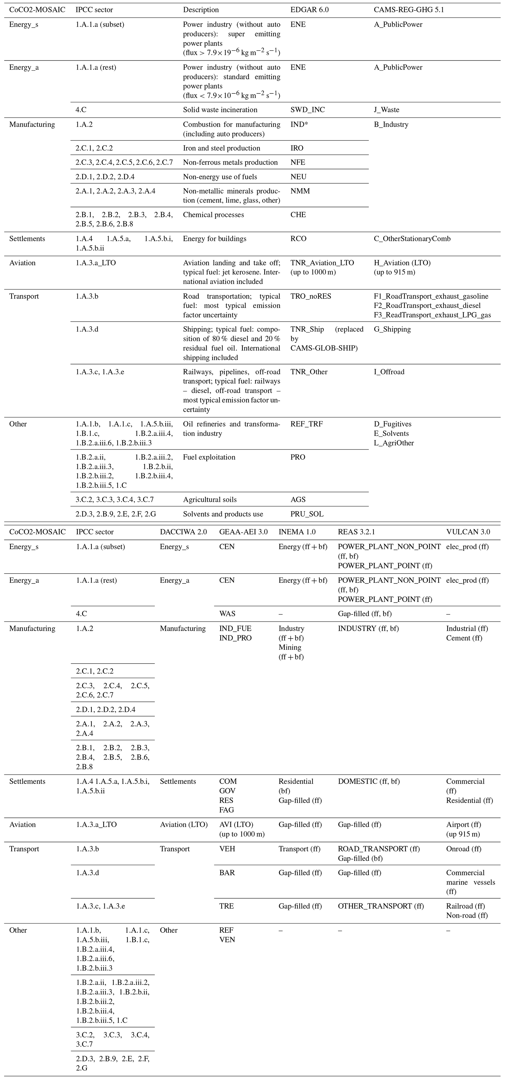
* Auto producers re-allocated from ENE to IND based on national statistics (Choulga et al., 2021).
2.2.4 Temporal re-distribution
All regional inventories provide monthly emissions except DACCIWA 2.0 and INEMA 1.0. In these inventories, monthly emissions were calculated based on CAMS-GLOB-TEMPO 3.1 monthly profiles: FM_ene_co2 for energy_s and energy_a (country specific), FM_ind for manufacturing (country specific), FM_res for settlements (pixel specific), and FM_tro for transport (country specific). Several countries share the same country-specific profiles in regions where fewer information is available (e.g., Africa). Flat profiles were used in sectors not covered by CAMS-GLOB-TEMPO 3.1: aviation and other.
2.2.5 Temporal gap-filling
CoCO2-MOSAIC 1.0 covers 2015, 2016, 2017, and 2018. The only year when all regional inventories are available is 2015. From 2016 to 2018, missing years were gap-filled with the latest year available in each regional inventory (see limitations in Sect. 5.8).
2.2.6 Masks
CoCO2-MOSAIC 1.0 includes a country and an inventory mask. The country mask is based on the Geographic Information System of the Commission (GISCO) 2020 dataset (1 m) (EUROSTAT, 2020). GISCO 2020 labels countries with their ISO alpha-3 codes and their English name. For rasterization, the ISO numeric (three-digit) code was used. At coastal borders, all pixels touching the coastal line were considered as land and assigned to the corresponding country (Fig. S2 in the Supplement). At country borders, pixels including more than one country were assigned to the country covering most of the border pixel (Fig. S3). Note that this could introduce a small error when using the country mask to aggregate the emissions per country in those countries with a significant share of their emissions close to their borders. These errors are negligible at the global scale, but users could use their own aggregation algorithms accounting for the exact area covered by each country to eliminate them.
The inventory mask maps each pixel to one input inventory (Fig. 1). In each country, regional inventories were used only if they covered the whole country, excluding overseas territories (Table S13). The spatial extent of regional inventories was limited to inland pixels (all pixels touching some land). Pixels fully covered by sea were assigned to the default global inventory (mainly shipping emissions from CAMS-GLOB-SHIP 3.1).
2.3 Complementary datasets
2.3.1 CO2ff aviation emissions from climb, descent, and cruise
Regional inventories only include LTO emissions, which are approximated by most inventories as aviation emissions emitted below 1 km (EDGAR and GEAA-AEI) or a roughly equivalent altitude of 3000′′ or 914 m (CAMS-REG-GHG and VULCAN). The remaining aviation emissions are calculated as the sum of EDGAR 6.0 climbing and descent (CDS) and cruise (CRS) sectors. Both domestic and international aviation are included. These emissions are provided in a separate file as they are not covered by regional inventories and are emitted into the atmosphere at different altitude.
2.3.2 LULUCF emissions
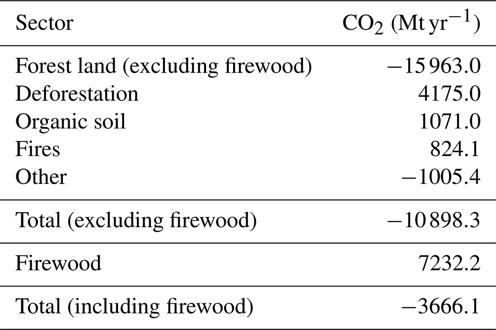
EDGAR LULUCF (Crippa et al., 2022) net fluxes are used to complete the overview of CO2 anthropogenic emissions. They are available at the regional level in five categories: “forest land” (living biomass), “deforestation”, “organic soil”, “fires”, and “other” (including all other land uses). EDGAR LULUCF provides independent estimates for the living biomass pool in forest land (including fires), while emissions from the other categories are based on a compilation of official country reports to the UNFCCC (Grassi et al., 2022). The forest land CO2 fluxes are obtained combining the forest area from satellite-derived land use data and the IPCC tier 1 approach, which uses IPCC default forest growth factors and country statistics on harvest. These fluxes are calculated over managed forests, derived from country information or approximated by means of a non-intact forest layer. Also biomass fire emissions are estimated by means of a tier 1 approach, using the Global Wildfire Information System (GWIS) burned area product (Artés et al., 2019). For this study, emissions from firewood harvest (preliminary estimate based on country statistics) were removed from forest land fluxes because these emissions are already accounted as CO2bf. A gridded EDGAR LULUCF dataset is not available yet, so LULUCF emissions are used for the analysis, but they are not integrated into CoCO2-MOSAIC 1.0.
3.1 Global emission inventories
Table 4 shows the global CO2 emission inventories benchmarked against CoCO2-MOSAIC 1.0. Note that CAMS-GLOB-ANT 5.3 (with the addition of DACCIWA 2.0) is the so-called CoCO2-PED 2018, i.e., the bottom-up inventory used as prior for CoCO2 global inversions. A full description of each inventory is available in the Supplement.
Table 4Description of the global inventories compared with CoCO2-MOSAIC 1.0.
3.2 Pre-processing
The global inventories were pre-processed as follows:
-
Spatial re-gridding: CAMS-GLOB-ANT 5.3, EDGAR 6.0, and CEDS v2021_04_21 are already available at the mosaic resolution. ODIAC v2020b (∘ × ∘) was directly averaged to 0.1∘ × 0.1∘. CAMS-GLOB-AIR 1.1 (0.5∘ × 0.5∘) were downscaled by replicating the 0.5∘ × 0.5∘ fluxes to the 0.1∘ × 0.1∘ grid.
-
Temporal resolution: all inventories provided monthly emissions.
-
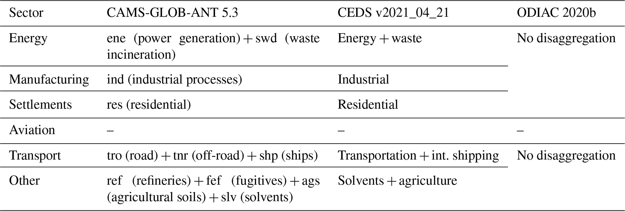
Sector aggregation: EDGAR sectors were already mapped to CoCO2-MOSAIC sectors (Table 3). The only difference is that, for the inter-comparison, EDGAR shipping emissions were used instead of CAMS-GLOB-SHIP 3.1. CAMS-GLOB-ANT 5.3 and CEDS v2021 sectors were aggregated as shown in Table 5. Aviation emissions are missing in CEDS, CAMS-GLOB-ANT, and ODIAC, at least in their highest resolution products. Some CEDS sectors do not fully match the definition of the corresponding mosaic sectors: energy emissions include fuel exploitation and transformation (accounted as “other” in the mosaic) and auto producers (accounted as “manufacturing” in the mosaic). Both CEDS and ODIAC only provide CO2ff emissions.
Table 5Sectorial re-aggregation of the global emission inventories for the inter-comparison. Sector definitions are available in the Supplement.
3.3 Inter-comparison methodology
The inter-comparison was made in 2015 as this is the only year when all regional inventories are simultaneously available. Monthly CO2ff and CO2bf emissions from CoCO2-MOSAIC 1.0 and the global inventories were compared per region. The aviation sector was treated separately (Sect. 2.3.3) because it is not provided by most global inventories. The energy_s and energy_a sectors were analyzed together to remove the influence of the different number of super-emitters in each inventory. The temporal disaggregation of the emissions was analyzed by comparing the monthly temporal factors (FT) per sector and CoCO2-MOSAIC region:
where emissions and emissions are the total monthly and annual emissions in each region and sector, respectively. The spatial disaggregation was assessed based on the annual spatial weight factors (FS) in each pixel per sector:
where emissions are the annual emission flux in each pixel and are the annual mean emission flux over the corresponding region. The spatial factors were based on the histograms of pixels with non-zero emissions. Both temporal and spatial factors were calculated separately for CO2ff and CO2bf.
3.3.1 Analysis of super-emitters
The number and magnitude of super-emitters (energy sources kg m−2 s−1) depend on the power and heat plant emissions (IPCC sector 1A1a), as well as the total number of emitting pixels, so we inter-compared both quantities per inventory and region. CEDS was excluded as the energy sector includes other activities besides power plant emissions. We used the CoCO2 1.0 global power plant database (Guevara et al., 2023) to analyze the geolocation of super-emitting pixels. We checked if super-emitting pixels contained a power plant, defining true positives (TP), i.e., super-emitters collocated with a power plant, false positives (FP), i.e., super-emitters not collocated with a power plant, and a special case of false positives (FP*), i.e., super-emitters not collocated with a power plant but with a power plant in one of the eight surrounding pixels. The last group was created to find potential geolocation errors either from the power plant database or from the global inventories.
3.3.2 Analysis of aviation emissions
Aviation emissions above 1 km were analyzed by comparing CoCO2-MOSAIC 1.0 (EDGAR 6.0 CDS + CRS) and CAMS-GLOB-AIR 1.1 (sum of the 23 levels above 1 km, from 1.525 to 14.945 km). For the aviation emissions below 1 km (LTO), we compared CoCO2-MOSAIC 1.0 with EDGAR 6.0 (LTO) and CAMS-GLOB-AIR 1.1 (first two levels: 305 and 915 m). We also evaluated the spatial allocation of LTO emissions in those regions where LTO emissions were available (USA, Europe, Argentina, and Africa), applying the same method used for super-emitters. CoCO2-MOSAIC 1.0 LTO emissions were used as the reference to define TP, a pixel with LTO emissions in both local and regional inventories, FP, a pixel with LTO emissions in the global inventory and no emissions in the regional one, and FN, a pixel with LTO emissions in the regional inventory and no emissions in the global one.
According to the Guide of the Expression of Uncertainty in Measurements (GUM) (JCGM, 2008), the pixel-level uncertainties of CoCO2-MOSAIC 1.0 should be calculated by propagating the pixel-level uncertainties of the input inventories through the different steps of the methodology. This would allow propagating CoCO2-MOSAIC uncertainties in inversion models and closing the uncertainty budget in comparisons with other inventories. Similarly, pixel-level uncertainties of input inventories should be obtained by propagating the uncertainties of their input datasets (country emissions, spatial and temporal proxies, etc.) through their models. However, we could not apply this methodology because, unfortunately, only VULCAN 3.0 provides pixel-level uncertainties. Instead, we used the methodology described by Choulga et al. (2021) to calculate the country level uncertainties based on the IPCC uncertainty framework (IPCC, 2006). For each IPCC sector, the methodology takes the IPCC default uncertainties for activity data and emission factors and propagates them first to EDGAR sectors and then to the CoCO2-MOSAIC sectors. CoCO2-MOSAIC 1.0 does not have this level of sector disaggregation. Thus, we combined the relative uncertainties reported by Choulga et al. (2021) for EDGAR sectors with EDGAR 6.0 emissions to calculate the relative uncertainty per CoCO2-MOSAIC sector and country, and then we applied CoCO2-MOSAIC 1.0 emissions to obtain the absolute uncertainties at country level. We split countries into well-developed (WDS) and less well-developed (LDS) statistical systems as made by Choulga et al. (2021). LDS uncertainties were also applied to emissions not covered by national inventories (shipping, aviation above 1 km). The methodology was only applied for CO2ff emissions due to the lack of default uncertainties for CO2bf. CO2bf uncertainty is expected to be larger due to less information available (Solazzo et al., 2021).
5.1 Description of CoCO2-MOSAIC 1.0
The total CO2 emissions in 2015 based on CoCO2-MOSAIC 1.0 are 36.7 Gt of CO2ff and 5.9 Gt of CO2bf (Table 6). These emissions are partly offset by a LULUCF sink of −10.9 Gt (Table 7). This sink is much bigger than the −3.7 Gt net LULUCF sink reported by Crippa et al. (2022) because here the emissions from firewood harvest (preliminarily estimated around +7.2 Gt, based on country statistics) have been removed from forest land, as these emissions are already counted as CO2bf emissions. The discrepancy between the +5.9 Gt of CO2bf and the +7.2 Gt of firewood harvests is due to the different years of harvest and burning, the additional sources of CO2bf besides firewood, and the different methodologies used by each dataset. Note that to calculate the total CO2 emissions according to the IPCC reporting guidelines, the 36.7 Gt (without CO2bf) should be added to the total sink of −3.7 Gt (without removing firewood harvest).
CO2ff emissions are driven by energy production (35.4 % of CO2ff), manufacturing (29.4 % of CO2ff), and transport (18.5 % of CO2ff). China, USA, India, Russia, Japan, and Germany are the largest emitters due to their large energy emissions, though manufacturing has the largest emission share in China and India. CO2bf emissions mainly come from settlements (55.9 % of CO2bf) and manufacturing (20.3 % of CO2bf), with India, Nigeria, and Brazil being the largest emitters. The LULUCF sink of −10.9 (or −3.7 Gt, including firewood) is driven by a forest land sink of −16.0 Gt (or −8.8 Gt, including firewood) partly offset by deforestation (+4.2 Gt) and organic soils (+1.1 Gt). The main contributors to the sink are large countries with a strong forest land sink: China, Russia, USA, and Canada. The largest LULUCF sources are Indonesia, driven by organic soils and deforestation, Brazil, driven by deforestation, and Australia, driven by fires. When LULUCF fluxes are normalized by the country extension, the largest relative sinks appear in central Africa (Gabon, Cameroon, Congo, and Central African Republic) due to a strong forest land sink. On the contrary, Ghana, Indonesia, Vietnam, Nigeria, and Brazil have the largest relative LULUCF sources due to deforestation.
Table 6Total CO2ff and CO2bf anthropogenic emissions per sector during 2015 based on CoCO2-MOSAIC 1.0.
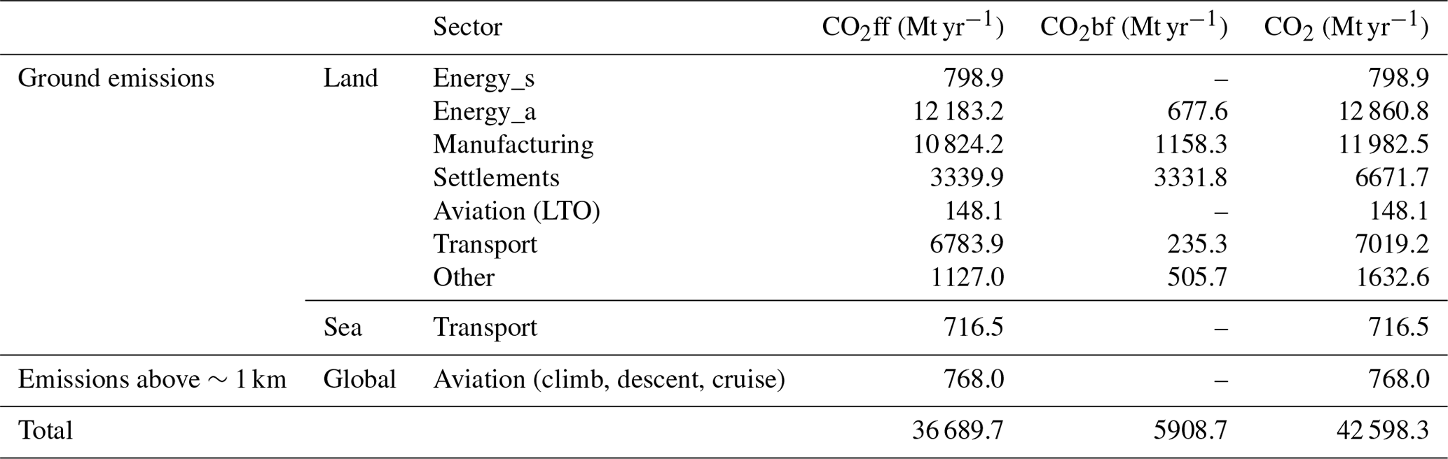
Table 7Net LULUCF CO2 flux during 2015 based on EDGAR-LULUCF.
5.2 Comparison of the inventories per region and sector
CoCO2-MOSAIC 1.0 has the largest CO2ff emissions overall (Fig. 5), which could be even larger due to not gap-filling regional inventories (VULCAN 3.0, REAS 3.2.1, and INEMA 1.0) in which “other” emissions were missing. The total “other” emissions in these regions are 1.3 Gt based on EDGAR 6.0, so despite that they may be partly included in other sectors, CoCO2-MOSAIC 1.0 emissions could be up to 3.7 % higher. The total CO2ff emissions of EDGAR 6.0 and CAMS-GLOB-ANT 5.3 are similar and just slightly smaller (<1 %) than those of CoCO2-MOSAIC 1.0. The sectorial emissions of EDGAR and CAMS-GLOB-ANT are also very consistent due to the strong dependence of CAMS-GLOB-ANT 5.3 on EDGAR 5.0. However, both diverge with CoCO2-MOSAIC 1.0 at the sector level: they have smaller emissions in the manufacturing (−14 % to −16 %, mainly REAS region) and transport (−7 % to −8 %, mainly USA and Europe) sectors, and larger emissions in the energy (+3 % to +4 %, mainly Europe and REAS region) and other (+137 % to +139 %, due to not gap-filling) sectors. CEDS v2021_04_21 has the smallest CO2ff emissions overall (−6.2 % of CoCO2-MOSAIC 1.1) and the largest discrepancies at the sector level due to the different definitions of the sectors. CEDS v2021_04_21 has the largest energy emissions (+2.2 Gt or +17.0 % of CoCO2-MOSAIC) because they include fuel exploitation and transformation (“other” in CoCO2-MOSAIC) and auto producers (“manufacturing” in CoCO2-MOSAIC). Consequently, both CEDS manufacturing (−2.3 Gt or −21.5 %) and “other” emissions (−1.0 Gt) are smaller. Despite the different sectorial aggregations, the total CEDS emissions in these sectors are −1.1 Gt smaller than those of the CoCO2-MOSAIC. The remaining difference is explained by the smaller emissions in settlements (−8.3 % than CoCO2-MOSAIC) and transport (−9.0 % than CoCO2-MOSAIC). ODIAC 2020b has also smaller CO2ff emissions than CoCO2-MOSAIC 1.0 (−3 %), CAMS-GLOB-ANT (−2 %), and EDGAR (−2 %), but larger than CEDS. Compared with the other global inventories, ODIAC has the smallest CO2ff emissions in Europe and the REAS region but the largest ones in the USA and Chile. ODIAC is the only gridded inventory not providing sectoral emissions to analyze the source of these discrepancies.
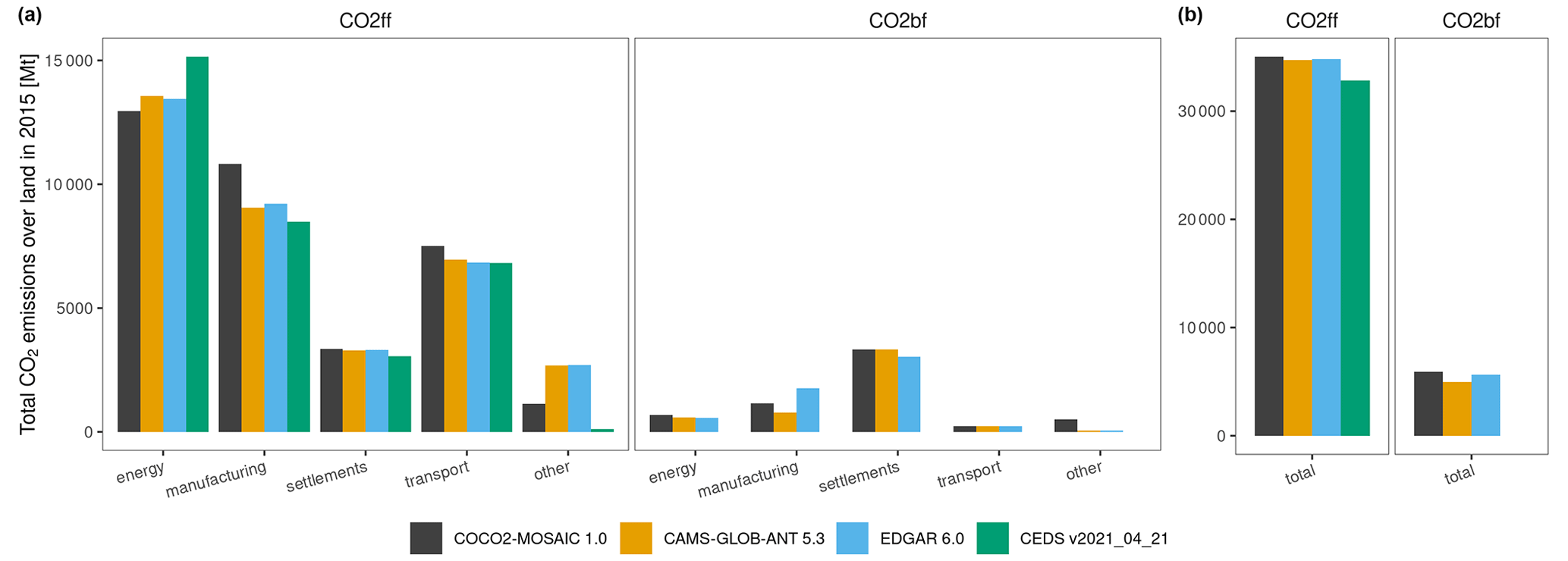
Figure 2Global CO2ff and CO2bf emissions in 2015 over land pixels: (a) per sector and (b) total. (Aviation LTO emissions are excluded.)
CoCO2-MOSAIC 1.0 also has the largest CO2bf emissions followed by EDGAR 6.0 (−4.1 %) and CAMS-GLOB-ANT 5.3 (−15.9 %). The difference between EDGAR and CAMS, not observed in CO2ff, is due to the large CO2bf manufacturing emissions of EDGAR 6.0. Compared with CoCO2-MOSAIC 1.0, EDGAR 6.0 has smaller CO2bf emissions in energy (−15.5 %) and other (−88.7 %) sectors, mainly due to differences in Africa and in the settlements sector (−8.8 %). On the contrary, EDGAR 6.0 has again larger CO2bf manufacturing emissions globally (+52.1 %) and in all the regions evaluated. This is due to the inclusion of emissions from bagasse in the food industry which were calculated from UN statistics in EDGAR. However, a better assessment of the uncertainty of these statistics is still needed. In EDGAR 6.0 the larger CO2bf manufacturing emissions can compensate partially the lower CO2bf settlements and energy emissions, like in the case of different sector allocations due to slightly different interpretations of definitions. Overall, the differences between inventories are larger in CO2bf than in CO2ff, especially over Africa or at the national level (Chile and Argentina), which could be linked to the less information available on biofuels emission.
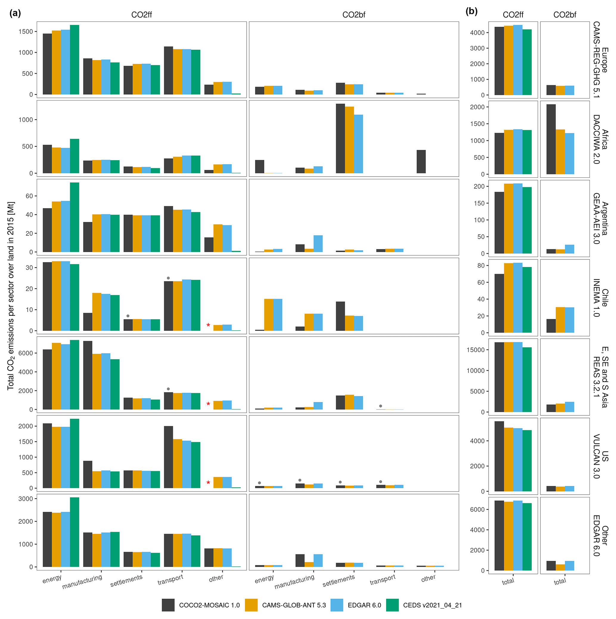
Figure 3Regional CO2ff and CO2bf emissions in 2015 over land pixels: (a) per sector and (b) total. Aviation LTO emissions are excluded. Red asterisks denote regions of the CoCO2-MOSAIC 1.0 with missing “other” emissions. Gray dots indicate CoCO2-MOSAIC 1.0 sectors fully or partly gap-filled with EDGAR 6.0.
The differences between inventories are analyzed per region and sector in Fig. 3. Note that differences in regions comprising many countries are biased towards countries with the largest emission share. Total and sectorial emissions are very similar in countries without a regional inventory, likely because all inventories use similar data sources due to the less information available in these countries. The main discrepancies are the abovementioned larger CO2bf manufacturing emissions by EDGAR 6.0 and the larger CO2ff energy emissions by CEDS.
The best agreement between regional and global inventories is observed in Europe and the REAS region. In both regions, the total emissions of the regional inventory are similar to those of EDGAR 6.0 and CAMS-GLOB-ANT 5.3, and +3 % to +7 % larger than those of ODIAC and CEDS. Some differences exist at the sector level. In Europe, compared with the global inventories, CAMS-REG-GHG 5.3 has larger CO2ff emissions in transport (all countries) and manufacturing (largest emitting countries except Turkey and Ukraine), smaller CO2ff emissions in energy (Germany, Great Britain, and Italy), and larger CO2bf emissions in settlements (all countries but France). In Asia, REAS 3.2.1 has the smallest energy emissions, the largest manufacturing emissions, and zero “other” emissions, but these differences cancel out so they may be partly explained by different sector definitions. Global inventories are also very consistent in the USA, but all of them have smaller (−6 % to −12 %) total CO2ff emissions than VULCAN 3.0 due to the larger regional emissions in the energy, manufacturing, and transport sectors. The larger manufacturing emissions of VULCAN are due to the inclusion of oil refineries and the transformation industry, which is included as “other” emissions in the global inventories and account for 272 out of 359 Mt CO2ff of the total “other” emissions in the USA (EDGAR estimates). This is also the only region where EDGAR and CAMS-GLOB-ANT emissions are smaller than ODIAC emissions, which suggests that both global inventories likely have too low emissions in this region.
Greater discrepancies are observed in Africa. Compared with global inventories, DACCIWA 2.0 has −0.1 Gt (−7 %) CO2ff emissions and +0.7 Gt (+58 %) CO2bf emissions, leading to a total positive difference of around +0.6 Gt of CO2. DACCIWA CO2ff is smaller due to its small “other” emissions (mostly in Algeria and Egypt). The greater DACCIWA CO2bf emissions are due to 264 Mt (energy) and 432 Mt (other) of CO2bf not accounted by any global inventory likely due to the exclusion of charcoal making emissions (Liousse et al., 2014).
The largest discrepancies are observed in national inventories. Both Argentinean and Chilean national inventories have the smallest CO2ff and CO2bf emissions. In Argentina, this is explained by the smaller GEAA-AEI 3.0 CO2ff emissions in the energy, manufacturing, and “other” sectors. Compared with global inventories, GEAA-AEI accounts for energy and manufacturing emissions as point sources, considering the direct fuel consumption at each power plant. In Chile, INEMA has smaller CO2ff emissions in manufacturing and “other” sectors and very low CO2bf emissions in the energy and manufacturing sectors. These CO2bf emissions were calculated with regional CO2ff CO2bf ratios, but this does not explain the observed differences because the total CO2 emissions of INEMA in these sectors are also smaller. The low INEMA manufacturing emissions, which are also lower than the national inventory values (Álamos et al., 2022), could be related to the use of the emissions self-reported by the companies to RETC. The smaller CO2bf emissions are likely due to the limited number of biofuels considered by INEMA but are partly offset by its large CO2bf settlements emissions due to a detailed accounting for domestic firewood consumption.
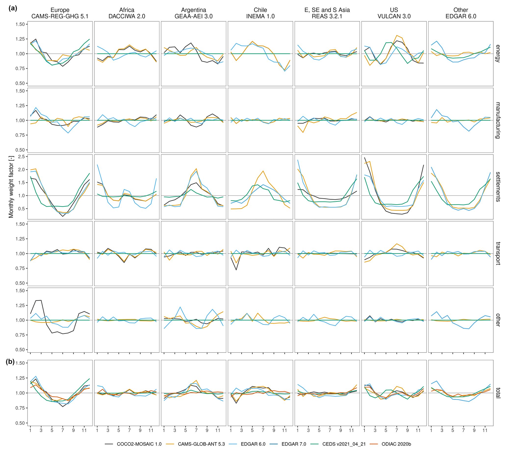
Figure 4Monthly CO2ff weight factors per sector and region in 2015. Factors are calculated with the total monthly emissions per region and sector (monthly weight factor = total monthly emissions per region total annual emissions per region). Note that the settlements sector has a different scale due to its larger seasonality.
5.3 Analysis of the temporal profiles
The total monthly profiles in CO2ff (Fig. 4) and CO2bf (Fig. S9) are driven by settlements (largest seasonality) and energy profiles (largest emissions and second largest seasonality). These two sectors have similar profiles in Europe, Chile, and Argentina, with a peak in their respective cold season, but differ in the USA, Asia, and Africa due to an additional peak during the warm season. All inventories gather these peaks and differ mostly in the magnitude of the oscillations. CEDS and ODIAC have the flattest profiles (completely flat in many sectors and regions), whereas the regional inventories and CAMS-GLOB-ANT 5.3 show the largest seasonality. Another notable difference is a lag of around 1 month in the CEDS temporal profiles that is observed in several sectors and regions. Note that the profiles from each inventory are independent: CAMS-GLOB-ANT 5.3 uses CAMS-GLOB-TEMPO 3.1, CEDS uses ECLIPSE profiles, ODIAC uses the seasonal changes of Andres et al. (2011), and EDGAR applies its own methodology.
A good agreement in the main sectors is again observed in Europe and Southeast Asia. The main discrepancy in Europe appears in “other” profiles, where the regional inventory shows a high seasonality not shown by global inventories. The temporal profiles of Southeast Asia are the flattest overall, mainly driven by those of China. This is also the only region where regional profiles are flatter than global ones. The main discrepancy in this region appears in the manufacturing sector, where CAMS-GLOB-ANT has a peak in December followed by a valley in January–February not shown by global inventories and likely related to a production peak at the end of the year. The agreement between CAMS-GLOB-ANT and the regional inventory is also good in the USA. On the contrary, the lag of CEDS is very evident and EDGAR 6.0 profiles are much flatter. The latter is clearly observed in the transport sector, where EDGAR 6.0 does not gather the summer peak shown by VULCAN and CAMS-GLOB-TEMPO.
The African profiles are mostly driven by northern African countries and South Africa. In Africa, both CAMS-GLOB-ANT 5.3 and DACCIWA 2.0 are based on CAMS-GLOB-TEMPO 3.1 and clearly differ from EDGAR 6.0 showing even opposite profiles (e.g., energy) likely due to the scarce temporal information available in this continent. The regional energy profile is mainly driven by South Africa seasonality where CAMS-GLOB-TEMPO indicates a winter (June–July) peak that contrasts to the summer (January) peak of EDGAR 6.0. In northern Africa, CAMS-GLOB-TEMPO shows a pronounced summer (July–August) peak, consistent with the increase in electricity demand for air cooling, not shown by EDGAR (except for Morocco). The agreement is better in the settlements sector, with both inventories showing a December–January peak in northern Africa and a June–July peak in South Africa, but the magnitude of EDGAR oscillations doubles those of CAMS-GLOB-TEMPO. Again, EDGAR and CAMS-GLOB-TEMPO have opposite profiles in the manufacturing sector because CAMS-GLOB-TEMPO applies country-specific profiles whereas EDGAR uses country-constant values. Both inventories also apply a country-constant profile in the transport sector due to the lack of information. (CAMS-GLOB-TEMPO applies TomTom congestion statistics mainly coming from South Africa.)
Chile and Argentina have similar temporal profiles due to their similar climatic conditions. Note that the regional profiles in Chile are based on CAMS-GLOB-TEMPO 3.1. In both countries, all the inventories show a decrease in the energy emissions in October–December and a winter (June–August) peak in the settlements sector consistent with heating consumption. Manufacturing profiles are quite flat except for those of the Argentina regional inventory, where the use of local data introduces a higher seasonality. A small discrepancy is also observed in the Chilean transport emissions in February. CAMS-GLOB-TEMPO (based on TomTom congestion statistics) shows a strong valley not gathered by EDGAR, which is consistent with a traffic reduction in Chilean cities during the holiday period.
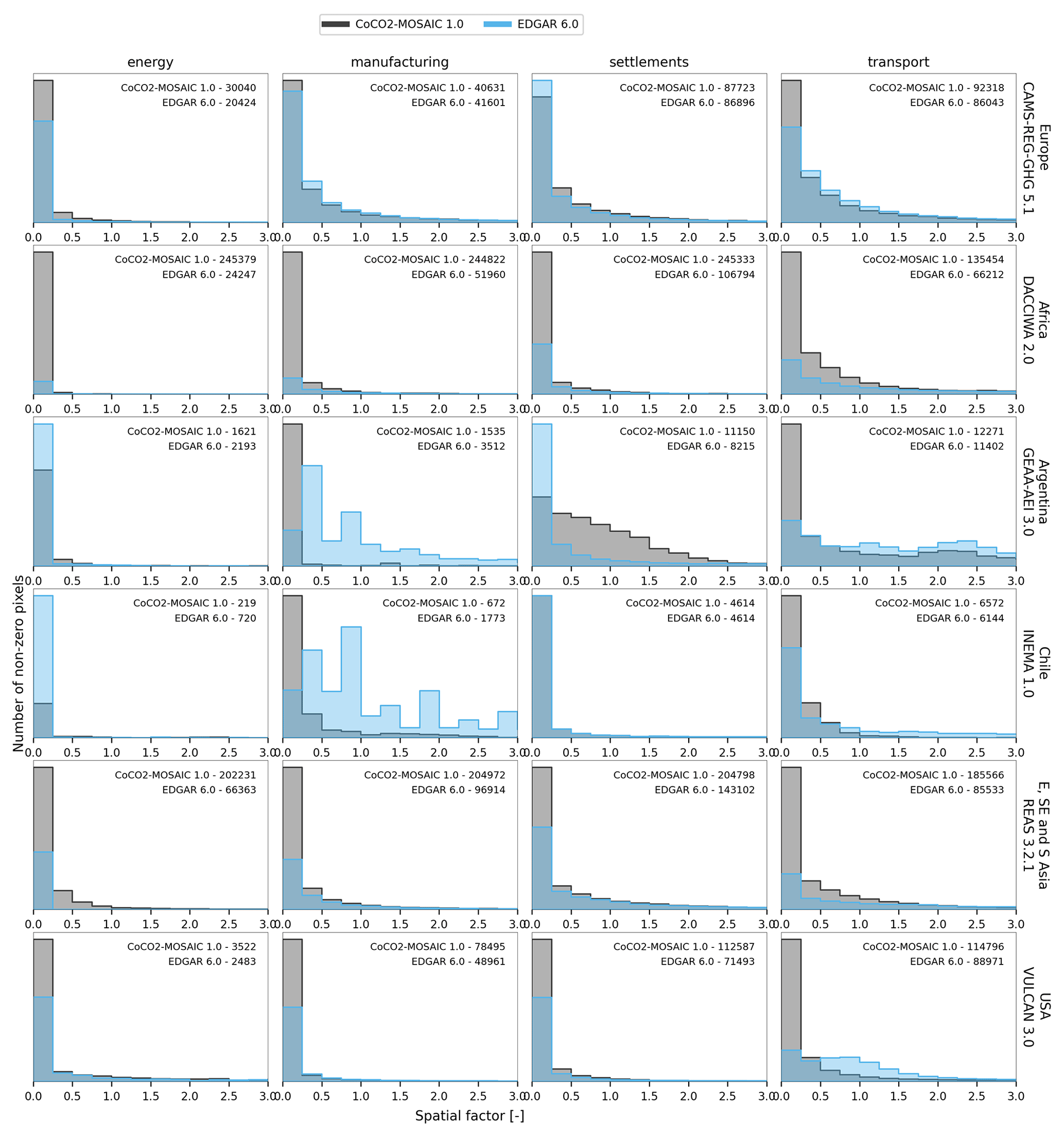
Figure 5Histogram of annual CO2ff spatial weight factors (pixel emission flux average emission flux in the region) during 2015 per region and sector. The annotation shows the number of pixels with non-zero emissions. Pixels with zero emissions are excluded from the histograms.
5.4 Analysis of the spatial disaggregation
The analysis of the spatial disaggregation for CO2ff (Fig. 5) and CO2bf (Fig. S10) focuses on the comparison of CoCO2-MOSAIC 1.0 with EDGAR 6.0 because both CAMS-GLOB-ANT 5.3 and CEDS v2020_04_21 are based on EDGAR spatial factors. CoCO2-MOSAIC 1.0 has more pixels with non-zero emissions than EDGAR 6.0 in most regions and sectors evaluated. The additional pixels of regional inventories have mostly low emissions (spatial weight factor <0.25). This pattern is only reversed when regional inventories provide the emissions as point sources (energy sector in Argentina and Chile, and manufacturing in Chile).
The best agreement is again observed in Europe, where the main discrepancy is the larger number of low-emitting pixels of CAMS-REG-GHG 5.3 in the energy and transport sectors. This pattern is also observed in Southeast Asia, the USA, and Africa. In Southeast Asia, the larger number of emitting pixels of REAS 3.2.1 is explained by the downscaling procedure applied to the original dataset (0.25∘ × 0.25∘), but otherwise, the distributions have similar shapes. The largest difference in the number of emitting pixels is observed in Africa. Figure S6 shows that all DACCIWA 2.0 pixels inside each country have non-zero emissions for the energy, manufacturing, and settlement sectors, due to disaggregating part of the emissions based on the population density. This procedure was not applied in the transport sector but the number of transport emitting pixels of DACCIWA 2.0 still doubles that of EDGAR 6.0, despite DACCIWA using EDGAR road network as a spatial proxy. The largest discrepancies are observed again in Chile and Argentina. Both national inventories have fewer non-zero pixels in the energy and manufacturing sectors due to the representation of power plants and manufacturing companies as point sources. Besides, the Argentinean settlements sector is the only one in all the regions evaluated where the regional inventory has a more uniform distribution than the global one. GEAA applies a bottom-up approach at very fine resolution estimating the consumption of census fractions up to 100–150 m in urban areas, which could explain the fewer number of emitting pixels and the more uniform distribution in GEAA.
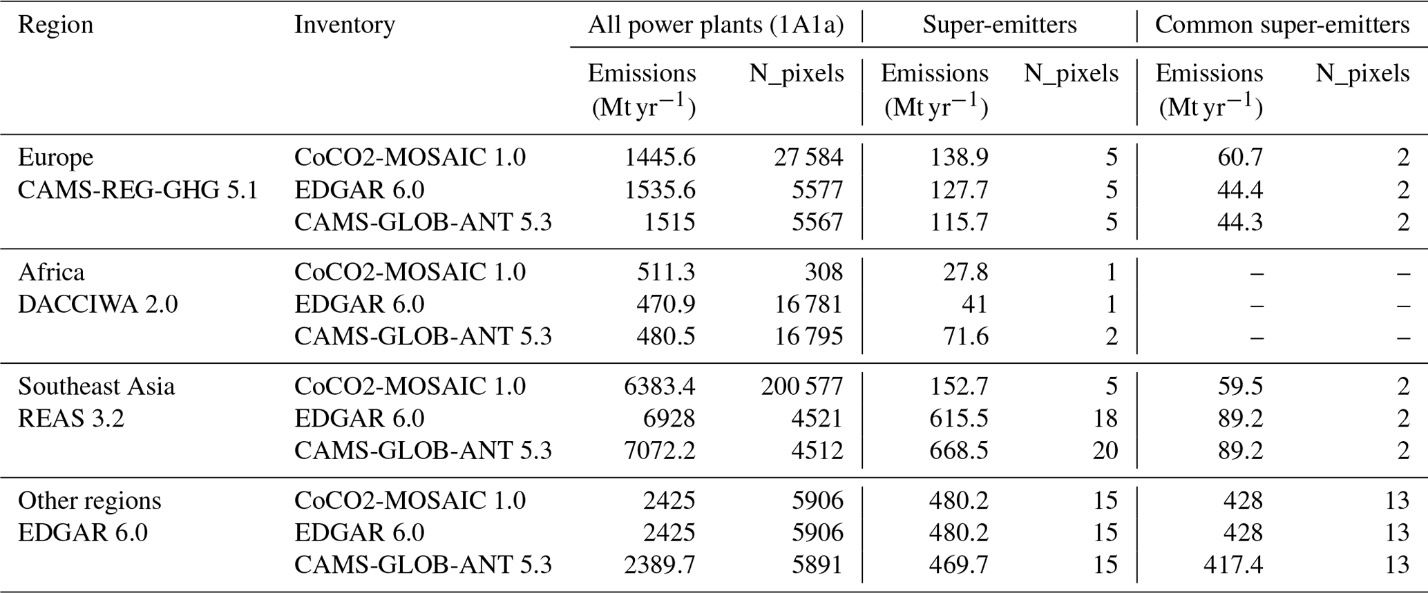
Table 8Summary of the super-emitting pixels (flux kg m−2 s−1) from each inventory per region. Regions without super-emitters are excluded. Common super-emitters are pixels identified as a super-emitter by all the inventories.
5.5 Analysis of super-emitting locations
The number and magnitude of the super-emitters in each inventory is a combination of (i) the magnitude of power plant emissions (1A1a) per country, (ii) the total number of emitting pixels, and (iii) the methodology used to spatially allocate these emissions. The emissions of the 1A1a sector have a small uncertainty, so in principle the regional differences between inventories should be small. This is true for Europe, but differences up to 10 % are observed between regional and global inventories in Southeast Asia and Africa (Table 8). However, the largest discrepancies are due to the different number of energy-emitting pixels in each inventory. Figure 6 analyzes the geolocation of super-emitting pixels by evaluating their agreement with the CoCO2 power plant database. Regional inventories have a perfect match with the power plant database, with all super-emitting pixels containing a power plant. By contrast, both EDGAR 6.0 and CAMS-GLOB-ANT 5.3 have six and eight false positives in the pixels covered by regional inventories. These cases are analyzed individually in Sect. S5 of the Supplement. Countries without regional inventories present the worst agreement likely due to the lower quality of both global inventories and global power plant databases in Russia and the Middle East. The total power plant emissions of global and regional inventories in Europe are similar, but CAMS-REG-GHG 5.1 has five times more emitting pixels than the global inventories likely due to the use of the CORINE land cover dataset to distribute emissions not linked to a specific point source. Despite this, the number of super-emitters in global and regional inventories is the same, and the magnitude of the regional super-emitting pixels is even 36 % greater in the two common super-emitters. All the super-emitters identified by CAMS-REG-GHG 5.1 contain a power plant, but CAMS-GLOB-ANT 5.3 and EDGAR 6.0 have the same false positive in Serbia. In Africa, the number of super-emitters identified by all the inventories is similar. All of them are in South Africa, but each inventory points out different super-emitters likely due to different geolocation errors in the global inventories. The largest discrepancies are observed in Asia. REAS 3.2.1 has 8.5 % less power plant emissions than EDGAR 6.0 spread over a much larger number of pixels (200 577 vs. 4521). This is partly due to the coarse native resolution of REAS 3.2.1. However, REAS 3.2.1 super-emitters are not influenced by the downscaling process because the most-emitting stations are available as point sources and were mapped directly to the 0.1∘ × 0.1∘ grid. Nevertheless, both the smaller power plant emissions and the higher number of energy sources could be the reason behind the smaller number of super-emitters in REAS (5 vs. 18–20). The use of the regional data significantly improves the agreement with the power plant database. All REAS super-emitters contain a power plant, whereas EDGAR 6.0 and CAMS-GLOB-ANT 5.3 have five and six false positives, respectively.
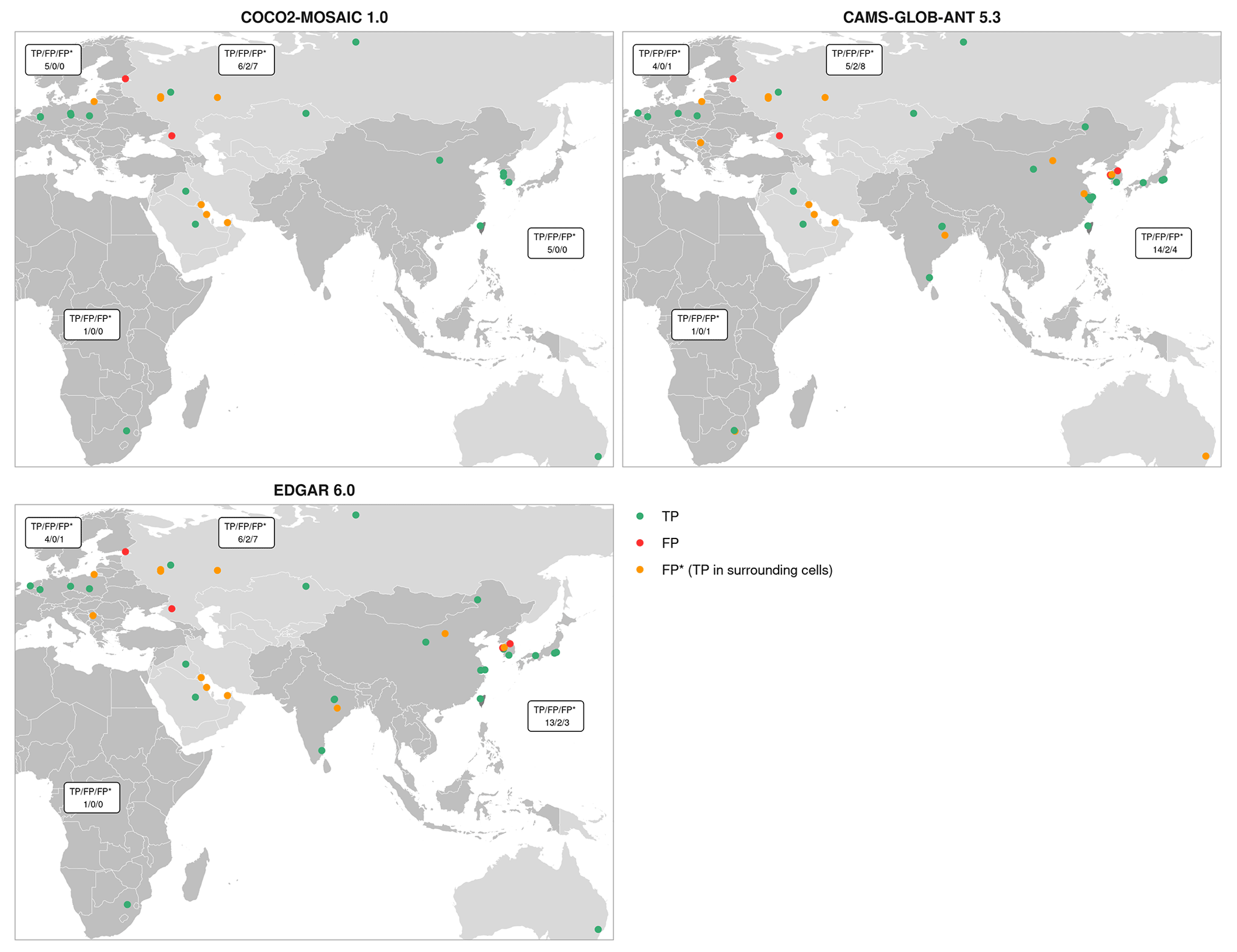
Figure 6Comparison of the location of super-emitting pixels from global inventories (test datasets) with the CoCO2 1.0 power plant database (reference dataset). TP: true positive; FP: false positive; FP*: false positive, with a TP in the surrounding pixels.
5.6 Analysis of aviation emissions
The aviation sector presents some of the largest discrepancies (Fig. 7). Global inventories have around 30 % fewer LTO emissions than CoCO2-MOSAIC 1.0 due to the larger emissions of regional inventories particularly in the USA. Furthermore, despite both global inventories having similar total LTO emissions, they have large discrepancies regionally. EDGAR 6.0 has larger emissions than CAMS-GLOB-AIR 1.1 in all the regions except for “Other countries”, where CAMS-GLOB-AIR LTO emissions are 60 % larger.
In addition, the climb, descent, and cruise (above ∼1 km) of CAMS-GLOB-AIR 1.1 are 14.7 % smaller than those of EDGAR 6.0, which also means that CAMS-GLOB-AIR total aviation emissions are smaller. CAMS-GLOB-AIR 1.1 is based on CEDS aviation emissions, but since 2014 it extrapolates linearly the 2012–2014 emissions. The International Energy Agency (IEA) statistics (IEA, 2022) show that, since 2014, both domestic and international aviation increased exponentially up to the COVID pandemic, which may explain the smaller CAMS-GLOB-AIR 1.1 emissions in 2015. Note also that the differences observed are also due to the different vertical profiles of each inventory. CoCO2-MOSAIC 1.0 takes EDGAR aviation emissions for consistency with the other sectors, but more detailed information on global vertical profiles can be found in Olsen et al. (2013).
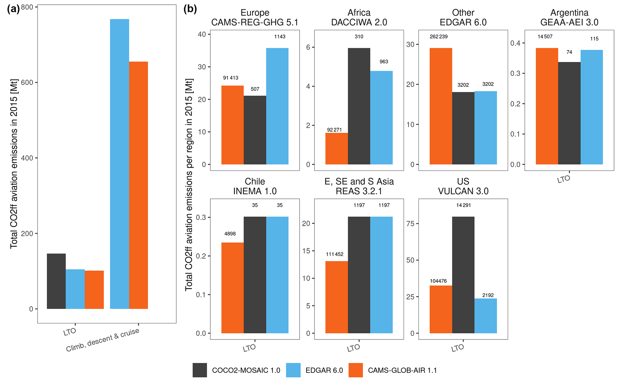
Figure 7Panel (a) shows a comparison of the total monthly aviation emissions globally from the different inventories. Panel (b) shows a comparison of the monthly aviation LTO emission per region. The annotation shows the number of pixels with LTO emissions. INEMA 1.0 and REAS 3.2.1 LTO emissions were gap-filled with EDGAR 6.0.
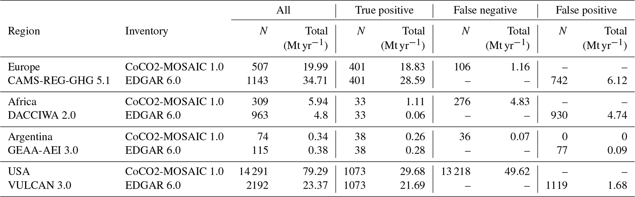
Table 8 analyzes the emissions in regions with LTO information. Europe is the only region EDGAR 6.0 LTO emissions are larger (+69.7 %) than those from the regional inventory, due to the larger emissions in pixels identified as LTO emitters by both inventories (28.6 vs. 18.8 Mt) and the additional number of LTO emitting pixels (1143 vs. 507, +6.1 Mt). In Africa, EDGAR 6.0 emissions are 19.6 % smaller than those of DACCIWA 2.0 despite EDGAR 6.0 having more LTO emitting pixels (963 vs. 309). Besides, Africa presents a very low number of true positives (pixels with LTO emissions in both inventories), which indicates a strong discrepancy between the spatial proxies of both inventories. In Argentina, GEAA-AEI 3.0 and EDGAR 6.0 show the best agreement regarding both the number of LTO emitting pixels and the magnitude of the emissions. The largest discrepancies are observed in the USA, with regional emissions being 2.4 times larger than global ones. VULCAN 3.0 emissions are around 1.5 times larger than those of EDGAR 6.0 in pixels identified as LTO emitters by both inventories (29.7 vs. 21.7 Mt), but the main difference is caused by the additional 13 218 LTO emitting pixels included by VULCAN 3.0 that add 49.62 Mt of CO2ff not accounted by EDGAR. This could be explained by the more extensive list of airports, including also helipads, used by VULCAN, whereas EDGAR uses a global database from the International Civil Aviation Organization (ICAO) that includes only the main airports and main flights.
Table 9CoCO2-MOSAIC 1.0 vs. EDGAR 6.0 aviation LTO emissions in regions with regional LTO information. N: number of pixels with LTO emissions; Total: annual LTO CO2 emissions during 2015.
5.7 Uncertainty analysis
The 95 % expanded uncertainty of CoCO2-MOSAIC 1.0 annual global CO2ff emissions in 2015 is (−1.24, 1.55 Gt) or (−3.4, 4.5 %). Manufacturing (−0.70, 1.08 Gt), aviation LTO (−0.38, 0.77 Gt), energy_a (−0.39, 0.42 Gt), transport (−0.31, 0.46 Gt), and other (−0.11, 0.48 Gt) are the sectors with the largest contribution (Table S16). The absolute uncertainty of the manufacturing sector is a combination of its large magnitude, which is driven by Chinese manufacturing emissions, and its large relative uncertainty (−6.5, 10 %), due to the large uncertainty of sub-sectors such as cement production. Aviation LTO has the second largest weight because we applied LDS uncertainties to global aviation emissions, which led to a relative uncertainty of (−50.1, 100.1 %). A high-relative uncertainty (−9.4, 42.8 %) also drives the contribution of “other” emissions in the total uncertainty.
Figure 8 presents the 20 countries with the largest contribution to global uncertainty. The main goal of this figure is to identify countries where the uncertainty can be more easily reduced to improve global estimates, either because they have a less well-developed statistical system or do not have regional, gridded information. Emission uncertainty can be particularly reduced in LDS countries without regional, gridded inventories: RUS, IRN, IRQ, MEX, KAZ, SAU, VEN, and BRA. The development of regional gridded inventories for Russia, the Middle East, and Latin America is highly needed to reduce the global uncertainty of bottom-up CO2 inventories. A second group of countries is covered by regional inventories but do not have a well-developed statistical system: KOR, ZAF, and NGA. Their uncertainty could be smaller than the values reported in this study based on LDS default uncertainties, due to the uptake of local information. This group also includes shipping emissions and aviation emissions above 1 km, which both have been considered as LDS. The high uncertainty of aviation emissions agrees with the large discrepancies observed in the previous section. More work is needed to reduce the uncertainty of global datasets of shipping and aviation emissions. The last group of countries with room for improvement includes Canada and Australia, the only countries with a well-developed statistical system without regional, gridded information. The development of gridded inventories for these countries could especially reduce the uncertainty of their spatially explicit emissions.
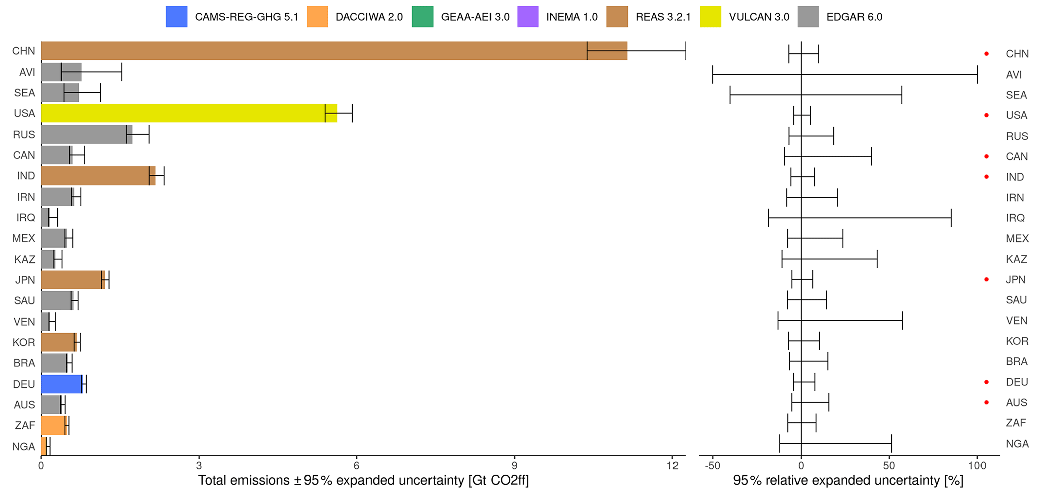
Figure 8Total emissions ±95 % expanded uncertainty and 95 % relative expanded uncertainty of CoCO2-MOSAIC 1.0 CO2ff emissions in the 20 countries with the largest absolute uncertainty. Countries are ranked top down according to their absolute uncertainty. Red dots indicate countries with a well-developed statistical system (WDS).
5.8 CoCO2-MOSAIC 1.0 limitations
The following limitations of CoCo2-MOSAIC have been identified:
-
Missing emissions. As mentioned above, VULCAN 3.0, REAS 3.2.1, and INEMA 1.0 emissions in the “other” sector are missing and have not been gap-filled to avoid double counting. The “other” emissions in these three inventories are 1.3 Gt yr−1 of CO2ff based on EDGAR 6.0. Despite that some of them are partly included in other sectors, CoCO2-MOSAIC 1.0 CO2ff emissions could be up to 3.7 % higher.
-
Spatial consistency. CoCO2-MOSAIC 1.0 emissions are not only spatially inconsistent between regions, but also inside those regions where global inventories have been used to gap-fill missing sectors (e.g., Chile and Southeast Asia).
-
Spatial coverage. CoCO2-MOSAIC 1.0 has global coverage, but regional inventories are missing in some regions with a high contribution to global CO2 emissions. The total uncertainty of the mosaic could be particularly reduced by developing regional, gridded inventories in Canada and Australia (among WDS countries) as well as Russia, the Middle East, and Latin America (among LDS countries).
-
Temporal coverage. CoCO2-MOSAIC 1.0 covers from 2015 to 2018, but only in 2015 are all regional inventories simultaneously available. Beyond 2015, regions with missing years (Chile, the USA, and Southeast Asia) were gap-filled with the last year available just for completeness. During this period, we recommend focusing on regions providing updated emissions. For more recent information on global CO2 emissions, we refer to CAMS-GLOB-ANT 5.3 (available up to 2023).
-
Other GHG species. CoCO2-MOSAIC 1.0 does not include CH4 and N2O. For these species, we refer again to CAMS-GLOB-ANT 5.3.
CoCO2-MOSAIC 1.0 is freely available at Zenodo (https://doi.org/10.5281/zenodo.7092358; Urraca et al., 2023) and at the JRC Data Catalogue (https://data.jrc.ec.europa.eu/dataset/6c8f9148-ce09-4dca-a4d5-422fb3682389; Urraca Valle et al., 2023) in NetCDF format. The main files include the monthly emissions per sector for one species (CO2ff and CO2bf) over 4 years (2015–2018). Three auxiliary layers are available: mask_inventory (inventory mask), mask_country (country mask), and cell_area (area of the grid cell). The aviation emissions above 1 km are provided as a separate file.
This paper presents CoCO2-MOSAIC 1.0, a mosaic of regional emission gridded inventories that provides CO2ff and CO2bf monthly emission fluxes from 2015 to 2018 disaggregated in seven sectors. The regional inventories integrated are CAMS-REG-GHG 5.1 (Europe), DACCIWA 2.0 (Africa), GEAA-AEI 3.0 (Argentina), INEMA 1.0 (Chile), REAS 3.2.1 (East, Southeast, and South Asia), and VULCAN 3.0 (USA). EDGAR 6.0, CAMS-GLOB-SHIP 3.1, and CAMS-GLOB-TEMPO 3.1 are used for gap-filling. CoCO2-MOSAIC 1.0 could be considered a globally accepted reference that can be recommended as a global baseline emission inventory. Based on this, we used CoCO2-MOSAIC 1.0 to inter-compare CAMS-GLOB-ANT 5.3, EDGAR 6.0, ODIAC v2020b, and CEDS v2020_04_24. The mosaic provides harmonized access to regional inventories at a global scale facilitating the replication of inter-comparisons such as the one made in this study.
CoCO2-MOSAIC has been used to benchmark global emission inventories identifying the main sources of discrepancy in each sector and region, giving valuable feedback to inventory developers to continue improving both regional and global emission datasets. CoCO2-MOSAIC 1.0 has the highest emissions overall (36.7 Gt of CO2ff, 5.9 Gt of CO2bf) despite not having gap-filled missing “other” emissions in some regions to avoid double-counting. Regional emissions are particularly larger than global ones in the USA (CO2ff) and Africa (CO2bf) and could be explained by the more complete information available at the regional level. All inventories represent the main seasonal changes, but regional inventories and CAMS-GLOB-TEMPO have higher seasonality that reflects better the local temporal patterns. Regional inventories generally disaggregate their emissions among a larger number of pixels, which could be also related to the use of region-specific spatial proxies. This pattern is the reverse in sectors such as energy or manufacturing, which are provided as point sources by most regional inventories. As a consequence, the agreement of regional inventories with the CoCO2 1.0 power plant database is better than for global inventories. All super-emitting pixels from regional inventories contained a power plant, whereas around 25 % of the super-emitters from global inventories were likely incorrectly geolocated. Some of the largest discrepancies were found in the aviation sector, both in the magnitude of the emissions and the spatial allocation of LTO emissions, which agrees with the large uncertainty reported in this sector. Finally, we estimated the overall uncertainty of mosaic emissions to identify sectors and countries where improvements could be more easily made to reduce the uncertainty of CO2 emissions at a global scale.
The supplement related to this article is available online at: https://doi.org/10.5194/essd-16-501-2024-supplement.
RU collected the data, developed the mosaic, and drafted the paper. GJM designed the mosaic and supervised the work. The mosaic was developed within the CoCO2 Task 2.1, which was composed by GJM, CG, HDvdG, MG, SK, and RU. HDvdG, StD, JK, and AV provided the European emissions. SK and SaD provided the African emissions. EP, ALN, and LBP provided the Argentinean emissions. NH and NÁ provided the Chilean emissions. KG and GR provided the emissions for the USA. CG and AV provided CAMS-GLOB-ANT emissions. MG provided the CAMS-GLOB-TEMPO profiles and the CoCO2 power plant database. GG and SR provided the LULUCF emissions. All the authors reviewed the manuscript. Apart from the first two authors, authors are listed in alphabetical order.
The contact author has declared that none of the authors has any competing interests.
Nicolas Huneeus acknowledges the FONDECYT project no. 1231717 and Research and Innovation programs, under grant agreement no. 870301 (AQ-WATCH).
Publisher's note: Copernicus Publications remains neutral with regard to jurisdictional claims made in the text, published maps, institutional affiliations, or any other geographical representation in this paper. While Copernicus Publications makes every effort to include appropriate place names, the final responsibility lies with the authors.
This research has been supported by the European Commission Prototype system for a Copernicus CO2 service (CoCO2), which received funding from the European Union's Horizon 2020 Research and Innovation Programme (grant no. 958927). Nicolás Huneeus was partially funded by the Science, Technology, Knowledge and Innovation Ministry of Chile through the FONDECYT program (grant no. 1231717) and by the AQ-WATCH project, which received funding from the European Union’s Horizon 2020 Research and Innovation Programme (grant no. 870301).
This paper was edited by Bo Zheng and reviewed by two anonymous referees.
Álamos, N., Huneeus, N., Opazo, M., Osses, M., Puja, S., Pantoja, N., Denier van der Gon, H., Schueftan, A., Reyes, R., and Calvo, R.: High-resolution inventory of atmospheric emissions from transport, industrial, energy, mining and residential activities in Chile, Earth Syst. Sci. Data, 14, 361–379, https://doi.org/10.5194/essd-14-361-2022, 2022.
Andres, R. J., Gregg, J. S., Losey, L., Marland, G., and Boden, T. A.: Monthly, global emissions of carbon dioxide from fossil fuel consumption, Tellus B, 63, 309–0327, https://doi.org/10.1111/j.1600-0889.2011.00530.x, 2011.
Artés, T., Oom, D., De Rigo, D., Durrant, T. H., Maianti, P., Libertà, G., and San-Miguel-Ayanz, J.: A global wildfire dataset for the analysis of fire regimes and fire behaviour, Sci. Data, 6, 296, https://doi.org/10.1038/s41597-019-0312-2, 2019.
Choulga, M., Janssens-Maenhout, G., Super, I., Solazzo, E., Agusti-Panareda, A., Balsamo, G., Bousserez, N., Crippa, M., Denier van der Gon, H., Engelen, R., Guizzardi, D., Kuenen, J., McNorton, J., Oreggioni, G., and Visschedijk, A.: Global anthropogenic CO2 emissions and uncertainties as a prior for Earth system modelling and data assimilation, Earth Syst. Sci. Data, 13, 5311–5335, https://doi.org/10.5194/essd-13-5311-2021, 2021.
Ciais, P., Crisp, D., Denier van der Gon, H., Engelen, R., Janssens-Maenhout, G., Rayner, P., and Scholze, M.: Towards a European Operational Observing System to Monitor Fossil CO2 Emissions, European Commission, Joint Research Centre, 65 pp., https://doi.org/10.2788/350433., 2015.
Crippa, M., Guizzardi, D., Muntean, M., Schaaf, E., Lo Vullo, E., Solazzo, E., Monforti-Ferrario, F., Olivier, J., and Vignatti, E.: EDGAR v6.0 Greenhouse Gas Emissions, European Commission [data set], http://data.europa.eu/89h/97a67d67-c62e-4826-b873-9d972c4f670b (last access: 1 April 2023), 2021.
Crippa, M., Guizzardi, D., Banja, M., Solazzo, E., Muntean, M., Schaaf, E., Pagani, F., Monforti-Ferrario, F., Olivier, J., Quadrelli, R., Risquez Martin, A., Taghavi-Moharamli, P., Grassi, G., Rossi, S., Jacome Felix Oom, D., Branco, A., San-Miguel-Ayanz, J., and Vignati, E.: CO2 emissions of all world countries – 2022 Report, European Commission, Joint Research Centre, https://doi.org/10.2760/730164, 2022.
Crippa, M., Guizzardi, D., Butler, T., Keating, T., Wu, R., Kaminski, J., Kuenen, J., Kurokawa, J., Chatani, S., Morikawa, T., Pouliot, G., Racine, J., Moran, M. D., Klimont, Z., Manseau, P. M., Mashayekhi, R., Henderson, B. H., Smith, S. J., Suchyta, H., Muntean, M., Solazzo, E., Banja, M., Schaaf, E., Pagani, F., Woo, J.-H., Kim, J., Monforti-Ferrario, F., Pisoni, E., Zhang, J., Niemi, D., Sassi, M., Ansari, T., and Foley, K.: The HTAP_v3 emission mosaic: merging regional and global monthly emissions (2000–2018) to support air quality modelling and policies, Earth Syst. Sci. Data, 15, 2667–2694, https://doi.org/10.5194/essd-15-2667-2023, 2023.
Dou, X., Wang, Y., Ciais, P., Chevallier, F., Davis, S. J., Crippa, M., Janssens-Maenhout, G., Guizzardi, D., Solazzo, E., Yan, F., Huo, D., Zheng, B., Zhu, B., Cui, D., Ke, P., Sun, T., Wang, H., Zhang, Q., Gentine, P., Deng, Z., and Liu, Z.: Near-real-time global gridded daily CO2 emissions, Innov., 3, 100182, https://doi.org/10.1016/j.xinn.2021.100182, 2022.
EUROSTAT: GISCO Countries 2020, European Commission, Eurostat [data set], 2020.
Granier, C., Darras, S., Denier van der Gon, H., Doubalova, J., Elguinidi, N., Galle, B., Gauss, M., Guevara, M., Jalkanen, J.-P., Kuenen, J., Liousse, C., Quack, B., Simpson, D., and Sindelarova, K.: The Copernicus Atmosphere Monitoring Service global and regional emissions (April 2019 version), Copernicus Atmosphere Monitoring Service (CAMS) report, Copernicus Atmosphere Monitoring Service (CAMS), https://doi.org/10.24380/d0bn-kx16, 2019.
Grassi, G., Conchedda, G., Federici, S., Abad Viñas, R., Korosuo, A., Melo, J., Rossi, S., Sandker, M., Somogyi, Z., Vizzarri, M., and Tubiello, F. N.: Carbon fluxes from land 2000–2020: bringing clarity to countries' reporting, Earth Syst. Sci. Data, 14, 4643–4666, https://doi.org/10.5194/essd-14-4643-2022, 2022.
Guevara, M., Jorba, O., Tena, C., Denier van der Gon, H., Kuenen, J., Elguindi, N., Darras, S., Granier, C., and Pérez García-Pando, C.: Copernicus Atmosphere Monitoring Service TEMPOral profiles (CAMS-TEMPO): global and European emission temporal profile maps for atmospheric chemistry modelling, Earth Syst. Sci. Data, 13, 367–404, https://doi.org/10.5194/essd-13-367-2021, 2021.
Guevara, M., Enciso, S., Tena, C., Jorba, O., Dellaert, S., Denier van der Gon, H., and Pérez García-Pando, C.: A global catalogue of CO2 emissions and co-emitted species from power plants at a very high spatial and temporal resolution, Earth Syst. Sci. Data Discuss. [preprint], https://doi.org/10.5194/essd-2023-95, in review, 2023.
Gurney, K. R., Liang, J., Patarasuk, R., Song, Y., Huang, J., and Roest, G.: The Vulcan Version 3.0 High-Resolution Fossil Fuel CO2 Emissions for the United States, J. Geophys. Res.-Atmos., 125, 27, https://doi.org/10.1029/2020JD032974, 2020.
Hoesly, R. M., Smith, S. J., Feng, L., Klimont, Z., Janssens-Maenhout, G., Pitkanen, T., Seibert, J. J., Vu, L., Andres, R. J., Bolt, R. M., Bond, T. C., Dawidowski, L., Kholod, N., Kurokawa, J.-I., Li, M., Liu, L., Lu, Z., Moura, M. C. P., O'Rourke, P. R., and Zhang, Q.: Historical (1750–2014) anthropogenic emissions of reactive gases and aerosols from the Community Emissions Data System (CEDS), Geosci. Model Dev., 11, 369–408, https://doi.org/10.5194/gmd-11-369-2018, 2018.
IEA: CO2 emissions in aviation in the Net Zero Scenario, 2000–2030, IEA, Paris, https://www.iea.org/data-and-statistics/charts/co2-emissions-in-aviation-in-the-net-zero-scenario-2000-2030 (last access: 1 April 2023), 2022.
IPCC: IPCC Guidelines for National Greenhouse Gas Inventories, edited by: Eggelston, S., Buendia, L., Miwa, K., Ngara, T., and Tanabe, K., Institute for Global Environmental Strategies (IGES), Hayama, Japan on behalf of the IPCC, Japan, ISBN 4-88788-032-4, 2006.
Janssens-Maenhout, G., Crippa, M., Guizzardi, D., Dentener, F., Muntean, M., Pouliot, G., Keating, T., Zhang, Q., Kurokawa, J., Wankmüller, R., Denier van der Gon, H., Kuenen, J. J. P., Klimont, Z., Frost, G., Darras, S., Koffi, B., and Li, M.: HTAP_v2.2: a mosaic of regional and global emission grid maps for 2008 and 2010 to study hemispheric transport of air pollution, Atmos. Chem. Phys., 15, 11411–11432, https://doi.org/10.5194/acp-15-11411-2015, 2015.
Janssens-Maenhout, G., Crippa, M., Guizzardi, D., Muntean, M., Schaaf, E., Dentener, F., Bergamaschi, P., Pagliari, V., Olivier, J. G. J., Peters, J. A. H. W., van Aardenne, J. A., Monni, S., Doering, U., Petrescu, A. M. R., Solazzo, E., and Oreggioni, G. D.: EDGAR v4.3.2 Global Atlas of the three major greenhouse gas emissions for the period 1970–2012, Earth Syst. Sci. Data, 11, 959–1002, https://doi.org/10.5194/essd-11-959-2019, 2019.
Janssens-Maenhout, G., Pinty, B., Dowell, M., Zunker, H., Andersson, E., Balsamo, G., Bézy, J.-L., Brunhes, T., Bösch, H., Bojkov, B., Brunner, D., Buchwitz, M., Crisp, D., Ciais, P., Counet, P., Dee, D., Denier van der Gon, H., Dolman, H., Drinkwater, M. R., Dubovik, O., Engelen, R., Fehr, T., Fernandez, V., Heimann, M., Holmlund, K., Houweling, S., Husband, R., Juvyns, O., Kentarchos, A., Landgraf, J., Lang, R., Löscher, A., Marshall, J., Meijer, Y., Nakajima, M., Palmer, P. I., Peylin, P., Rayner, P., Scholze, M., Sierk, B., Tamminen, J., and Veefkind, P.: Toward an Operational Anthropogenic CO2 Emissions Monitoring and Verification Support Capacity, B. Am. Meteorol. Soc., 101, E1439–E1451, https://doi.org/10.1175/BAMS-D-19-0017.1, 2020.
JCGM: JCGM 100:2008. Evaluation of measurement data – Guide to the expression of uncertainty in measurement, Geneve, Joint Committee for Guides in Metrology, Bureau International des Poids et Mesures, 2008.
Johansson, L., Jalkanen, J.-P., and Kukkonen, J.: Global assessment of shipping emissions in 2015 on a high spatial and temporal resolution, Atmos. Environ., 167, 403–415, https://doi.org/10.1016/j.atmosenv.2017.08.042, 2017.
Keita, S., Liousse, C., Assamoi, E.-M., Doumbia, T., N'Datchoh, E. T., Gnamien, S., Elguindi, N., Granier, C., and Yoboué, V.: African anthropogenic emissions inventory for gases and particles from 1990 to 2015, Earth Syst. Sci. Data, 13, 3691–3705, https://doi.org/10.5194/essd-13-3691-2021, 2021.
Kuenen, J., Dellaert, S., Visschedijk, A., Jalkanen, J.-P., Super, I., and Denier van der Gon, H.: CAMS-REG-v4: a state-of-the-art high-resolution European emission inventory for air quality modelling, Earth Syst. Sci. Data, 14, 491–515, https://doi.org/10.5194/essd-14-491-2022, 2022.
Kurokawa, J. and Ohara, T.: Long-term historical trends in air pollutant emissions in Asia: Regional Emission inventory in ASia (REAS) version 3, Atmos. Chem. Phys., 20, 12761–12793, https://doi.org/10.5194/acp-20-12761-2020, 2020.
Li, M., Liu, H., Geng, G., Hong, C., Liu, F., Song, Y., Tong, D., Zheng, B., Cui, H., Man, H., Zhang, Q., and He, K.: Anthropogenic emission inventories in China: a review, Natl. Sci. Rev., 4, 834–866, https://doi.org/10.1093/nsr/nwx150, 2017.
Liousse, C., Assamoi, E., Criqui, P., Granier, C., and Rosset, R.: Explosive growth in African combustion emissions from 2005 to 2030, Environ. Res. Lett., 9, 035003, https://doi.org/10.1088/1748-9326/9/3/035003, 2014.
Liu, Z., Ciais, P., Deng, Z., Davis, S. J., Zheng, B., Wang, Y., Cui, D., Zhu, B., Dou, X., Ke, P., Sun, T., Guo, R., Zhong, H., Boucher, O., Bréon, F.-M., Lu, C., Guo, R., Xue, J., Boucher, E., Tanaka, K., and Chevallier, F.: Carbon Monitor, a near-real-time daily dataset of global CO2 emission from fossil fuel and cement production, Sci. Data, 7, 392, https://doi.org/10.1038/s41597-020-00708-7, 2020a.
Liu, Z., Ciais, P., Deng, Z., Lei, R., Davis, S. J., Feng, S., Zheng, B., Cui, D., Dou, X., Zhu, B., Guo, R., Ke, P., Sun, T., Lu, C., He, P., Wang, Y., Yue, X., Wang, Y., Lei, Y., Zhou, H., Cai, Z., Wu, Y., Guo, R., Han, T., Xue, J., Boucher, O., Boucher, E., Chevallier, F., Tanaka, K., Wei, Y., Zhong, H., Kang, C., Zhang, N., Chen, B., Xi, F., Liu, M., Bréon, F.-M., Lu, Y., Zhang, Q., Guan, D., Gong, P., Kammen, D. M., He, K., and Schellnhuber, H. J.: Near-real-time monitoring of global CO2 emissions reveals the effects of the COVID-19 pandemic, Nat. Commun., 11, 5172, https://doi.org/10.1038/s41467-020-18922-7, 2020b.
McDuffie, E. E., Smith, S. J., O'Rourke, P., Tibrewal, K., Venkataraman, C., Marais, E. A., Zheng, B., Crippa, M., Brauer, M., and Martin, R. V.: A global anthropogenic emission inventory of atmospheric pollutants from sector- and fuel-specific sources (1970–2017): an application of the Community Emissions Data System (CEDS), Earth Syst. Sci. Data, 12, 3413–3442, https://doi.org/10.5194/essd-12-3413-2020, 2020.
Meijer, Y., Boesch, H., Bombelli, A., Brunner, D., M, B., P, C., D, C., R, E., Holmulnd, K., S, H., Janssens-Maenhout, G., Marshall, J., Nakajima, M., Pinty, B., Scholze, M., Bezy, J., Drinkwater, M., Fehr, T., Fernandez, V., Loescher, A., Nett, H., and Sierk, B.: Copernicus CO2 Monitoring Mission Requirements Document, European Space Agency, EOP-SM/3088/YM-ym, 2020.
Oda, T., Maksyutov, S., and Andres, R. J.: The Open-source Data Inventory for Anthropogenic CO2, version 2016 (ODIAC2016): a global monthly fossil fuel CO2 gridded emissions data product for tracer transport simulations and surface flux inversions, Earth Syst. Sci. Data, 10, 87–107, https://doi.org/10.5194/essd-10-87-2018, 2018.
Olsen, S. C., Wuebbles, D. J., and Owen, B.: Comparison of global 3-D aviation emissions datasets, Atmos. Chem. Phys., 13, 429–441, https://doi.org/10.5194/acp-13-429-2013, 2013.
Pinty, B., Janssens-Maenhout, G., Dowell, M., Zunker, H., Brunhes, T., Ciais, P., Dee, D., Denier van der Gon, H., Dolman, H., Drinkwater, M., Engelen, R., Heimann, M., Holmulnd, K., Husband, R., Kentarchos, A., Meijer, Y., Palmer, P., and Scholze, M.: An Operational Anthropogenic CO2 Emissions Monitoring & Verification Support capacity – Baseline Requirements, Model Components and Functional Architecture, European Commission, Joint Research Centre, https://doi.org/10.2760/39384, 2017.
Pinty, B., Ciais, P., Dee, D., Holman, D., Dowell, M., Engelen, R., Holmlund, K., Janssens-Maenhout, G., Meijer, Y., Palmer, P., Scholze, M., Denier van der Gon, H., Heimann, M., Juvyns, O., Kentarchos, A., and Zunke, H.: An Operational Anthropogenic CO2 Emissions Monitoring & Verification Support Capacity – Needs and high level requirements for in situ measurements, European Commission, Joint Research Centre, https://doi.org/10.2760/182790, 2019.
Puliafito, S. E., Bolaño-Ortiz, T. R., Fernandez, R. P., Berná, L. L., Pascual-Flores, R. M., Urquiza, J., López-Noreña, A. I., and Tames, M. F.: High-resolution seasonal and decadal inventory of anthropogenic gas-phase and particle emissions for Argentina, Earth Syst. Sci. Data, 13, 5027–5069, https://doi.org/10.5194/essd-13-5027-2021, 2021.
Sierk, B., Fernandez, V., Bézy, J.-L., Meijer, Y., Durand, Y., Bazalgette Courrèges-Lacoste, G., Pachot, C., Löscher, A., Nett, H., Minoglou, K., Boucher, L., Windpassinger, R., Pasquet, A., Serre, D., and te Hennepe, F.: The Copernicus CO2M mission for monitoring anthropogenic carbon dioxide emissions from space, in: International Conference on Space Optics – ICSO 2020, 128, https://doi.org/10.1117/12.2599613, 2021.
Solazzo, E., Crippa, M., Guizzardi, D., Muntean, M., Choulga, M., and Janssens-Maenhout, G.: Uncertainties in the Emissions Database for Global Atmospheric Research (EDGAR) emission inventory of greenhouse gases, Atmos. Chem. Phys., 21, 5655–5683, https://doi.org/10.5194/acp-21-5655-2021, 2021.
Soulie, A., Granier, C., Darras, S., Zilbermann, N., Doumbia, T., Guevara, M., Jalkanen, J.-P., Keita, S., Liousse, C., Crippa, M., Guizzardi, D., Hoesly, R., and Smith, S.: Global Anthropogenic Emissions (CAMS-GLOB-ANT) for the Copernicus Atmosphere Monitoring Service Simulations of Air Quality Forecasts and Reanalyses, Earth Syst. Sci. Data Discuss. [preprint], https://doi.org/10.5194/essd-2023-306, in review, 2023.
Urraca, R., Jansens-Maenhout, G., der Gon, H. D. Van, Dellaert, S., Kuenen, J., Visschedijk, A., Granier, C., Soulie, A., Keita, S., Darras, S., Guevara, M., Puliafito, E., Lopez-Noreña, A., Berna-Peña, L., Huneeus, N., Álamos, N., Gurney, K., Roest, G., Grassi, G., Rossi, S., Gobron, N., and Dowell, M.: CoCO2-MOSAIC 1.0: a global mosaic of regional, gridded, fossil and biofuel CO2 emission inventories, Zenodo [data set], https://doi.org/10.5281/zenodo.7092359, April 2023.
Urraca Valle, R., Janssens-Maenhout, G., Denier Van der Gon, H., Dellaert, S., Kuenen, J., Visschedijk, A., Granier, C., Soulie, A., Keita, S., Darras, S., Guevara, M., Puliafito, E., Lopez-Noreña, A., Berna-Peña, L., Huneeus, N., Álamos, N., Gurney, K., Roest, G., Grassi, G., Rossi, S., Gobron, N., and Dowell, M.: CoCO2-MOSAIC 1.0: a global mosaic of regional, gridded, fossil and biofuel CO2 emission inventories, European Commission, Joint Research Centre (JRC) [data set], http://data.europa.eu/89h/6c8f9148-ce09-4dca-a4d5-422fb3682389 (last access: 15 May 2023), 2023.
Zheng, B., Tong, D., Li, M., Liu, F., Hong, C., Geng, G., Li, H., Li, X., Peng, L., Qi, J., Yan, L., Zhang, Y., Zhao, H., Zheng, Y., He, K., and Zhang, Q.: Trends in China's anthropogenic emissions since 2010 as the consequence of clean air actions, Atmos. Chem. Phys., 18, 14095–14111, https://doi.org/10.5194/acp-18-14095-2018, 2018.