AIGD-PFT: the first AI-driven global daily gap-free 4 km phytoplankton functional type data product from 1998 to 2023

Long time series of spatiotemporally continuous phytoplankton functional type (PFT) data are essential for understanding marine ecosystems and global biogeochemical cycles as well as for effective marine management. In this study, we integrated artificial intelligence (AI) technology with multisource marine big data to develop a spatial–temporal–ecological ensemble model based on deep learning (STEE-DL). This model generated the first AI-driven global daily gap-free 4 km PFT chlorophyll a concentration product from 1998 to 2023 (AIGD-PFT). The AIGD-PFT significantly enhances the accuracy and spatiotemporal coverage of quantifying eight major PFTs: diatoms, dinoflagellates, haptophytes, pelagophytes, cryptophytes, green algae, prokaryotes, and Prochlorococcus. The model input encompasses (1) physical oceanographic, biogeochemical, and spatiotemporal information and (2) ocean colour data (OC-CCI v6.0) that have been gap-filled using a discrete cosine transform–penalized least squares (DCT-PLS) approach. The STEE-DL model utilizes an ensemble strategy with 100 residual neural network (ResNet) models, applying Monte Carlo and bootstrapping methods to estimate the optimal PFT chlorophyll a concentration and assess the model uncertainty through ensemble means and standard deviations. The model's performance was validated using multiple cross-validation strategies – random, spatial-block, and temporal-block methods – combined with in situ data, demonstrating STEE-DL's robustness and generalization capability. The daily updates and seamless nature of the AIGD-PFT data product capture the complex dynamics of coastal regions effectively. Finally, through a comparative analysis using a triple-collocation analysis (TCA) approach, the competitive advantages of the AIGD-PFT data product over existing products were validated. The complete product dataset (1998–2023) can be freely downloaded from https://doi.org/10.11888/RemoteSen.tpdc.301164 (Zhang and Shen, 2024a).

1 Introduction

Marine phytoplankton contribute to approximately half of the Earth's primary productivity (Field et al., 1998), driving the operation of marine ecosystems (Beaugrand et al., 2010). These minute organisms are classified into different phytoplankton functional types (PFTs), playing a crucial role in global biogeochemical cycles, biodiversity, and climate feedbacks (Le Quéré et al., 2005; Gruber et al., 2019). Comprehensive monitoring and research with respect to the spatiotemporal distribution patterns of PFTs are foundational for understanding marine ecosystems and predicting the impacts of climate change (Kramer et al., 2024; Falkowski, 2012). Particularly, for the accurate quantification of global ocean carbon fluxes and the improvement of biogeochemical models (Guidi et al., 2016), long-term, high-resolution PFT data are a scientific priority (Nair et al., 2008). Furthermore, as human reliance on marine resources increases, ensuring the sustainability of fisheries (Chassot et al., 2010), the effective management of coastal areas, and the protection of these regions from the risks posed by harmful algal blooms (Xi et al., 2023a) all underscore the value of the phytoplankton diversity data represented by PFTs (Henson et al., 2021).

For the quantification of global PFTs, many analytical techniques and inversion algorithms have been developed in recent years. Among the field sampling analysis methods for quantifying the global phytoplankton community composition from water samples, including optical microscopy (Karlson et al., 2010), flow cytometry (Veldhuis and Kraay, 2000), and recent genomics (Catlett et al., 2020), the separation of phytoplankton diagnostic pigments through high-performance liquid chromatography (HPLC) with the assistance of diagnostic pigment analysis (DPA; Vidussi et al., 2001) or CHEMTAX (Mackey et al., 1996) algorithms remains the most cost-effective and quality-controlled method to date (Swan et al., 2016). The advent of ocean colour satellites has enabled continuous global observation. In situ HPLC pigment data and ocean colour satellite data have laid the foundation for the development of remote sensing inversion methods, primarily including abundance-based and spectral-based approaches (Mouw et al., 2017; Bracher et al., 2017). Abundance-based indirect methods use the chlorophyll a (Chl a) concentration as model input, modelling the statistical relationship between the Chl a concentration and diagnostic pigments to retrieve PFTs globally (Hirata et al., 2011; Uitz et al., 2006). Spectral-based methods directly construct relationships between remote sensing reflectance, or absorption spectra, scattering spectra, and the concentrations of different functional types, incorporating spectral transformation strategies, such as principal component analysis (Xi et al., 2020) and differential spectra (Bracher et al., 2009), to improve inversion accuracy (Sun et al., 2022). Considering that marine ecological environmental variables (e.g. temperature and nutrients) shape the distribution of different functional types through their impact on phytoplankton growth, physiology, and competition, introducing more marine environmental covariates into ecological approaches (Zhang et al., 2023; Raitsos et al., 2008; El Hourany et al., 2024; Li et al., 2023) has become a current research focus: further introducing other biogeochemical and physical oceanographic data on the basis of ocean colour satellite data and integrating advanced machine learning methods like random forests and ensemble learning can significantly enhance the accuracy of PFT modelling.

Table 1 Summary of existing open-source PFT Chl a data products.

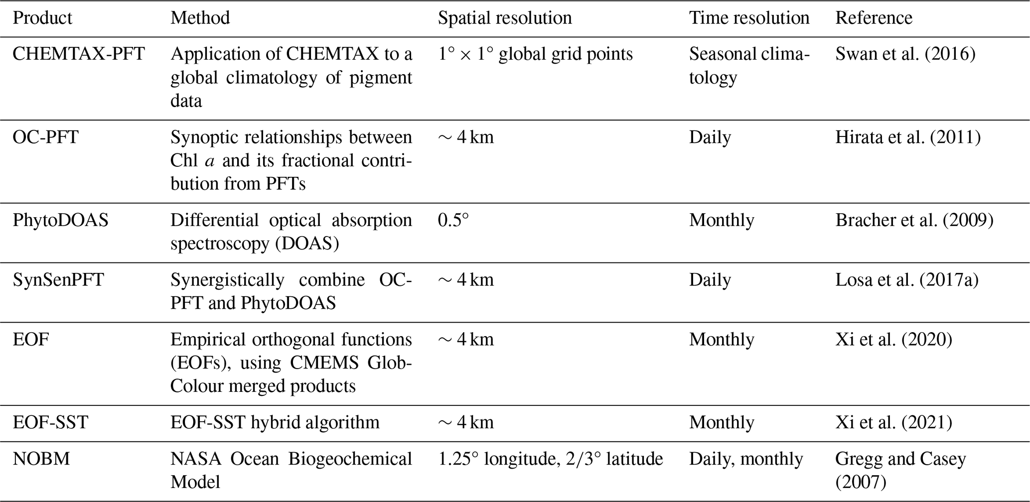
Based on the aforementioned approaches, several global PFT Chl a concentration products have been developed (Table 1), including the following: (1) a global seasonal surface marine climatology dataset based on CHEMTAX and a global HPLC dataset (Swan et al., 2016); (2) the OC-PFT product based on abundance (Hirata et al., 2011); (3) the PhytoDOAS product based on phytoplankton differential optical absorption spectroscopy (Bracher et al., 2009); (4) the synergistic product SynSenPFT that integrates satellite multispectral information with retrievals based on high-resolution PFT absorption properties derived from hyperspectral satellite measurements (Losa et al., 2017a); (5) the EOF-PFT product based on remote sensing reflectance and the empirical orthogonal functions (EOFs) algorithm (Xi et al., 2020), along with its modification, the EOF-SST hybrid algorithm (Xi et al., 2021), which incorporates sea surface temperature (SST). In addition to these remote sensing products, the NASA Ocean Biogeochemical Model (NOBM, https://gmao.gsfc.nasa.gov/reanalysis/MERRA-NOBM/data/data_description.php, last access: 21 October 2024) has been developed, which couples circulation and radiative models (Gregg and Casey, 2007).

Despite advancements in current algorithms for the retrieval of PFTs, significant challenges persist in terms of prediction accuracy, spatial coverage, and spatiotemporal resolution. First, abundance-based methods, which rely on Chl a remote sensing products and empirical formulas to deduce the composition of various PFTs, are computationally straightforward but suffer from limited accuracy and robustness globally (Bracher et al., 2017). Spectral-based methods encounter challenges because of the spectral resolution limitations of current ocean colour satellites, which restrict their ability to detect weak phytoplankton signals in optically complex waters. In such environments, non-algal particulate absorption and significant near-infrared water reflectance can obscure diagnostic pigment absorption, potentially rendering spectral-based methods ineffective (Nair et al., 2008). Another significant limitation is the presence of data gaps due to unfavourable conditions, such as orbital configurations, cloud cover, sunlight contamination, and large sensor viewing angles (Mikelsons and Wang, 2019). For instance, the probability of cloud-free conditions over the global ocean for MODIS is only between 25 % and 30 % (Liu and Wang, 2018). Although merging images from different satellite missions (e.g. MODIS, VIIRS, and OLCI) into merged products, such as OC-CCI (Sathyendranath et al., 2019) and CMEMS GlobColour (Garnesson et al., 2019), has effectively reduced data gaps, the issue of data loss remains severe. This not only results in numerous voids in PFT Chl a products but may also introduce biases in trend analysis, obscuring key signals of environmental change and hindering a comprehensive understanding of marine ecosystem dynamics. Such limitations restrict potential applications in climate change research and marine health monitoring. Monthly averaging of data can mitigate the issue of missing data to some extent. However, this approach may conceal significant short-term ecological changes, such as ocean heat waves (Chauhan et al., 2023) and algal blooms (Sadeghi et al., 2012). Additionally, the absence of data also limits the full utilization of on-site data: due to the incompleteness of remote sensing data, many in situ data cannot be effectively paired with them. This results in the potential inability of models to fully utilize on-site sampling data for calibration or optimization, thereby wasting expensive sampling resources and possibly diminishing the model's generalization capability (Xi et al., 2020). While biogeochemical models offer a global, spatiotemporally continuous PFT modelling approach, their spatial resolution often lacks the detail necessary to accurately reflect local changes and the dynamic characteristics of marine ecosystems.

In summary, although there have been positive developments, current PFT models and products have an imbalance in accuracy, spatiotemporal resolution, spatial coverage, and temporal span when compared with existing requirements, suggesting that there is still room for improvement in terms of practicality. The advent of the ocean big-data era, coupled with the rise of artificial intelligence technologies such as machine learning, offers new prospects for overcoming the inherent challenges faced by PFT inversion models that currently rely solely on ocean colour satellite data (Zhang et al., 2023). Algorithms for data reconstruction and the integration of multisource data can effectively bridge the observational gaps caused by clouds or orbital configurations, enhancing data utilization efficiency and the continuity of global phytoplankton community monitoring. Furthermore, the application of machine learning and deep learning technologies has the potential to improve the extraction of useful information from vast oceanic datasets. These technologies, capable of processing and analysing large-scale datasets to identify complex patterns and trends, hold the promise of developing high-precision PFT Chl a data products.

Here, we propose a novel spatial–temporal–ecological ensemble model based on deep learning (STEE-DL), designed to produce a long-time-series PFT Chl a data product. STEE-DL leverages an ensemble of 100 residual neural network (ResNet) models, incorporating inputs from reconstructed missing ocean colour data, physical reanalysis, and biogeochemical and spatiotemporal information. Utilizing the STEE-DL model, we have produced the first AI-driven global daily gap-free 4 km resolution phytoplankton functional type data product (AIGD-PFT), including eight major PFTs (i.e. diatoms, dinoflagellates, haptophytes, pelagophytes, cryptophytes, green algae, prokaryotes, and Prochlorococcus) from 1998 to 2023. The STEE-DL model's accuracy has been tested using three types of cross-validation (CV): standard, spatial-block, and temporal-block CV. Moreover, we have performed a comprehensive comparison and validation of the AIGD-PFT against other products using triple-collocation analysis (TCA).

2 Methodology

2.1 Overall framework

The structure and function of phytoplankton communities are influenced by numerous environmental factors, such as sunlight, nutrient concentration/supply, temperature, carbon chemistry characteristics, and their fluid dynamic environment. We regard the inversion process of PFTs as a nonlinear mapping (f_x) problem, aiming to overcome the limitations of relying solely on bio-optical algorithms for predicting the spatial distribution of phytoplankton. This process integrates environmental predictive factors (p), including bio-optical properties, biogeochemical parameters, physical conditions, and spatiotemporal factors, as shown in Eq. (1):

$$\begin{array}{}\text{(1)}& \mathrm{\text{PG}}=f_x\left(p_{\text{Bio-optical}},p_{\mathrm{Biogeochemical}},p_{\mathrm{Physical}},p_{\text{Spatiotemporal}}\right).\end{array}$$

Building on the work of Zhang et al. (2023), this study further modifies and constructs a STEE-DL model based on a ResNet ensemble to establish f_x. An overview of the proposed approach is shown in Fig. 1. It specifically includes the following:

1. Based on the global in situ HPLC dataset compiled by Zhang et al. (2023), this study has expanded and updated the aforementioned dataset to increase the quantity and diversity of the in situ data.

2. To address the issue of missing OC data, we utilized the discrete cosine transform–penalized least squares (DCT-PLS) method to reconstruct the data and fill in the missing pixel values.

3. We have integrated multiple sources of marine environmental data as input variables for the regression model.

4. Addressing the complex supervised regression problem encountered in multisource data processing, we trained an ensemble of 100 ResNet models, named the STEE-DL model, to generate daily PFT Chl a data products for the period from 1998 to 2023.

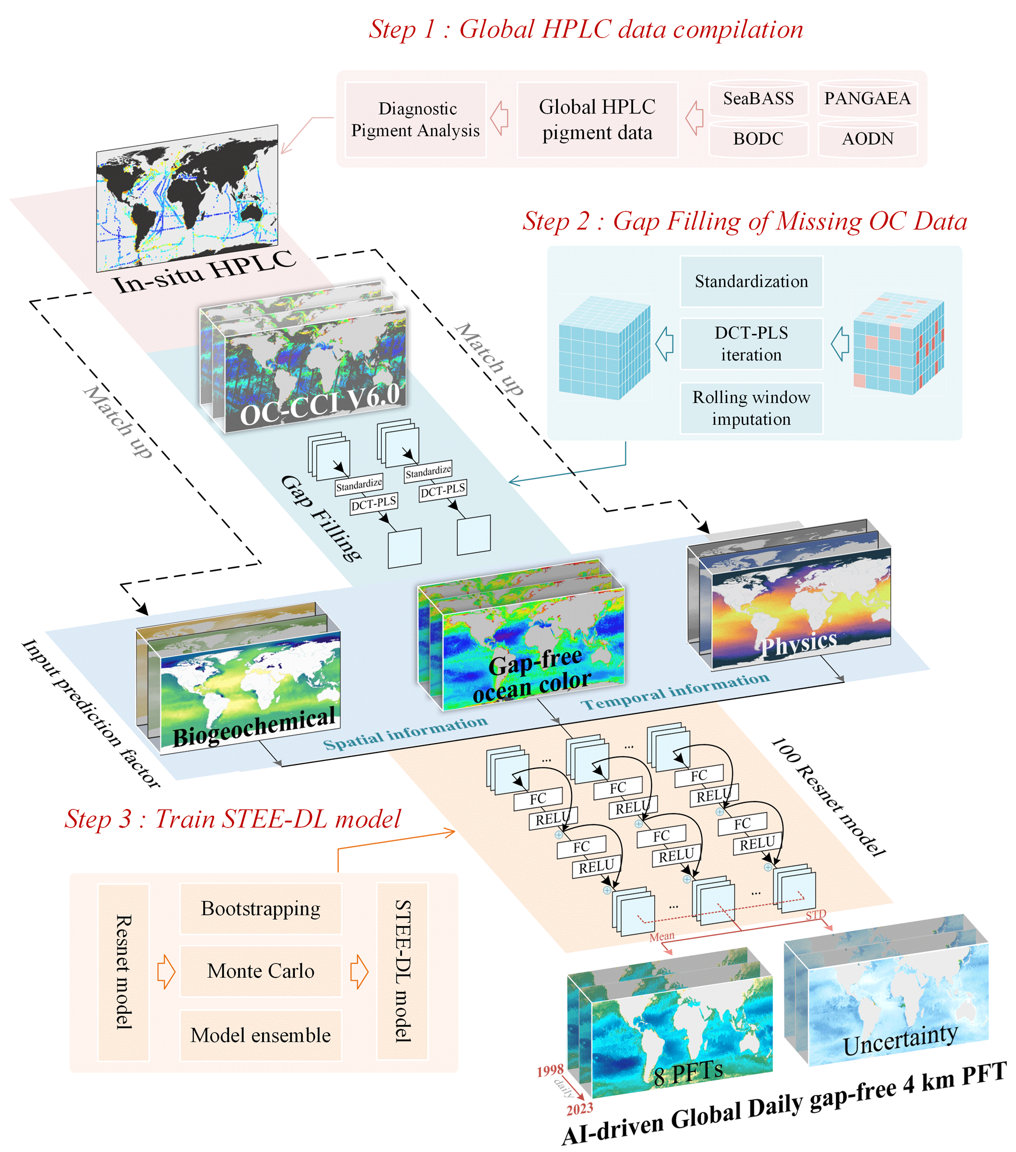
Figure 1 Schematic flow of the methodological approach in this study.

2.2 Input datasets and preprocessing

We first compiled and integrated in situ data obtained by HPLC and then collected predictor data including ocean colour data, physical oceanography data, and biogeochemistry data for model training and product generation.

2.2.1 HPLC pigment data

Building upon the updates presented by Zhang et al. (2023), this study integrates additional, newly available HPLC pigment data collected between 1998 and 2023 (refer to Fig. 2 for details). These data were primarily sourced from open-access data repositories such as SeaBASS (https://seabass.gsfc.nasa.gov/, last access: 21 October 2024), PANGAEA (https://www.pangaea.de/, last access: 21 October 2024), the British Oceanographic Data Centre (BODC, https://www.bodc.ac.uk/, last access: 21 October 2024), the Australian Ocean Data Network (AODN, https://portal.aodn.org.au/, last access: 21 October 2024), and Google Dataset Search (https://datasetsearch.research.google.com/, last access: 21 October 2024). This initiative has resulted in the acquisition of further HPLC open-source data, leading to the creation of a new global in situ HPLC pigment database spanning the years from 1998 to 2023 (see Table S1 in the Supplement). In cases of duplicate samples, whether across spatial or temporal dimensions, the average of the replicates was calculated. By utilizing an updated diagnostic pigment analysis (DPA) methodology, along with newly adjusted weighting coefficients, we conducted DPA to ascertain in situ PFT Chl a concentrations. Following conventional practice in the field (Xi et al., 2020, 2021), this analysis includes eight major PFTs: diatoms, dinoflagellates, haptophytes, pelagophytes, cryptophytes, green algae, prokaryotes, and Prochlorococcus. The adjusted coefficients for DPA were referenced from Alvarado et al. (2022) and Xi et al. (2023a), with specifics available at https://doi.org/10.1594/PANGAEA.954738 (Xi et al., 2023b). From these global HPLC pigment datasets, we selected six long-term observation sites as independent validation data. The locations of these sites are shown in Fig. 2.

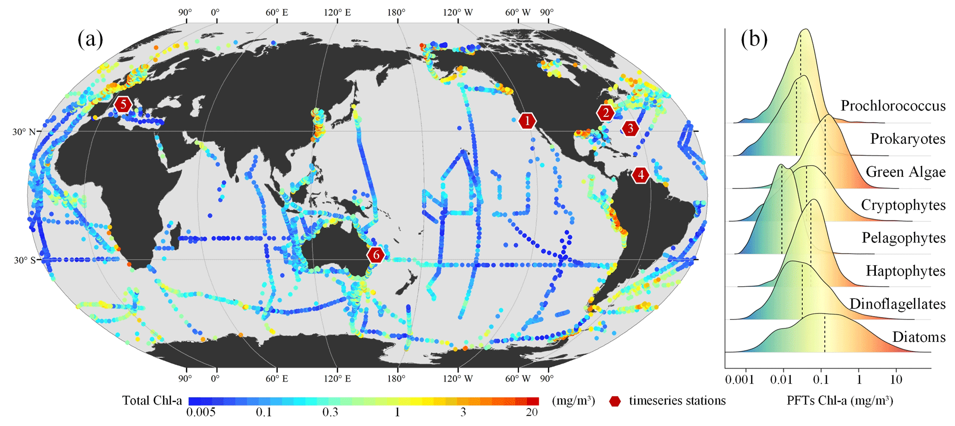
Figure 2 Panel (a) depicts the spatial distribution of in situ HPLC pigment datasets, with red hexagons and numbers indicating the locations of six independent stations with long-term time series. Panel (b) presents a ridge plot of the probability density distribution for eight types of PFTs.

2.2.2 Ocean colour data and missing value filling

Satellite ocean colour remote sensing data are currently the most important source for the retrieval of PFTs. We obtained daily merged ocean colour data from the Ocean-Colour Climate Change Initiative (OC-CCI, version 6.0, https://www.oceancolour.org/, last access: 21 October 2024) for the period from 1998 to 2023. These data combine measurements from the SeaWiFS, MERIS, MODIS-Aqua, and VIIRS sensors and have a spatial resolution of 4 km (Sathyendranath et al., 2019). The raw daily OC-CCI dataset exhibits considerable instances of missing data: Fig. 3a illustrates the percentage of valid pixels in the OC-CCI dataset, based on per-pixel statistics spanning the years from 1998 to 2023. The results indicate that the majority of marine areas exhibit less than 50 % coverage of valid observations, with pronounced gaps particularly evident at higher latitudes.

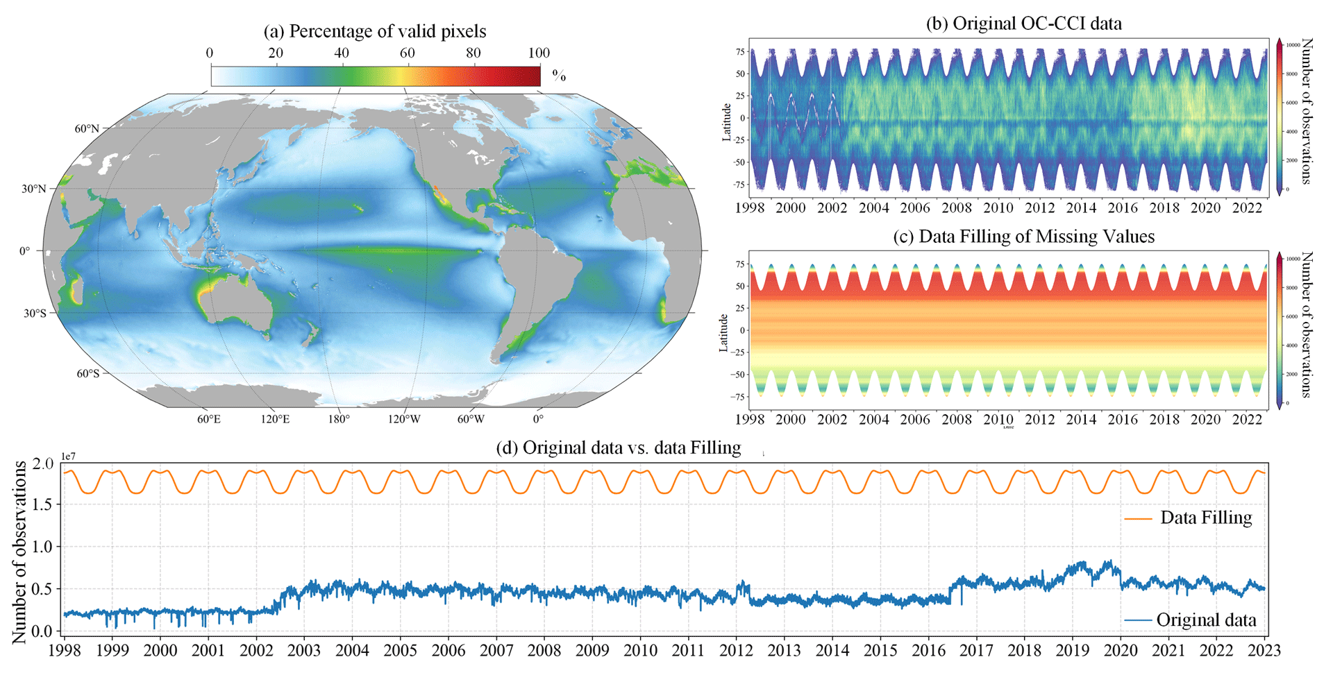
Figure 3 (a) Percentage of valid pixels in the OC-CCI v6.0 daily dataset. Hovmöller diagrams of (b) original OC-CCI data and (c) data after gap filling using the DCT-PLS method. (d) Comparison of the number of valid pixels between reconstructed and original data.

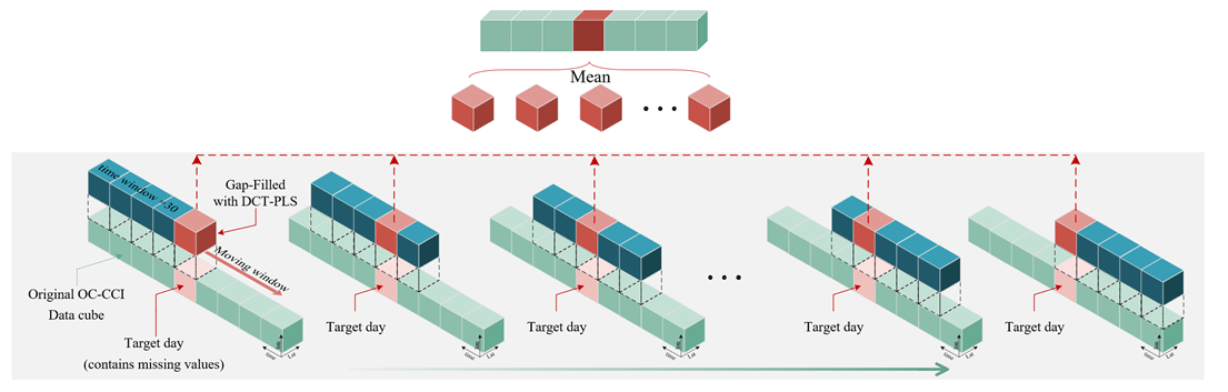
Given the importance of ocean colour data in generating seamless space–time PFT Chl a data products, they are essential to reprocess missing pixels to fill gaps, thereby maximizing the availability of in situ and remote sensing data. Previous studies have developed various methods for reconstructing missing pixels in remote sensing data, such as DINEOF (data interpolation empirical orthogonal function; Alvera-Azcárate et al., 2011; Liu and Wang, 2022), optimal interpolation (Liston and Elder, 2006), and Kriging (Gunes et al., 2006). However, these methods are very time-consuming when dealing with large datasets. For long-term and daily product reconstructions, balancing accuracy and computational efficiency is crucial. Therefore, we adopted the DCT-PLS algorithm, which was initially proposed for the automatic smoothing of multidimensional incomplete data (Garcia, 2010). The primary advantage of the DCT-PLS is its faster speed; moreover, it requires only a small amount of memory storage and achieves high reconstruction accuracy, making it suitable for processing large datasets. It has been successfully applied to fill data gaps in soil moisture (Wang et al., 2012), NDVI (normalized difference vegetation index; Yang et al., 2022), coastal ocean surface current (Fredj et al., 2016), and Chl a (Wang et al., 2022) products. To further improve the computational efficiency of the DCT-PLS algorithm, we modified the original DCT-PLS code, utilizing the built-in fast Fourier transform (FFT) computation in PyTorch for GPU-accelerated DCT operations.

Based on the DCT-PLS algorithm, we designed a gap-filling process (as shown in Fig. 4), which is briefly summarized as follows:

1. Data preparation. The original ocean satellite data (e.g. OC-CCI remote sensing reflectance R_rs, Chl a concentration, and diffuse attenuation coefficient K_d490) are stored in a three-dimensional spatiotemporal data cube. To avoid seams, we directly input the entire global 30 d data cube, with dimensions of $\mathrm{4320}\times \mathrm{8640}\times \mathrm{30}$, representing spatial resolution and a 30 d date–time span, without using regional segmentation.

2. Normalization. To minimize differences in dimensions and magnitudes of data across different spatial regions, the dataset is standardized by dividing by the spatial mean. The spatial mean is calculated from the entire dataset spanning from 1998 to 2023.

3. DCT-PLS completion. The DCT-PLS method is used to fill in missing values for the target day. We modified the original code of Garcia (2010) (https://www.mathworks.com/matlabcentral/fileexchange/27994-inpaint-over-missing-data-in-1-d-2-d-3-d-nd-arrays?s_tid=prof_contriblnk, last access: 21 October 2024) to a GPU-accelerated form, significantly improving speed compared with the original MATLAB-based code. The entire 30 d time series of data underwent 100 iteration cycles in the DCT-PLS process to fill in the missing values for the target date.

4. Rolling filling. To enhance the robustness of the filling effect, we adopt a rolling filling strategy. Specifically, for each target day, a 30 d time window is progressively moved forward day by day until the data window moves past that day. This process is repeated 30 times for each target day, with the average of these fillings taken as the final result for the target day.

5. Long-time-series filling. Following the process described, the entire dataset is traversed and filled day by day, ultimately resulting in a daily continuous and spatially complete data cube from 1998 to 2023.

This method effectively utilizes time-series information to estimate missing values while avoiding discontinuities that might be introduced by data segmentation. Through iteration and averaging, it further improves the accuracy and stability of the filled data. Additionally, via GPU acceleration, this method achieves higher efficiency compared with traditional methods (such as DINEOF). It is important to note that these data will be directly removed (as demonstrated in the video example available at https://doi.org/10.5446/67366, Zhang, 2024) in high-latitude areas (above 75°) with extremely high missing rates (exceeding 80 %), as reconstruction under such conditions is impractical.

Figure 4 Gap-filling process with the DCT-PLS algorithm.

Table 2 Predictors and corresponding data products.

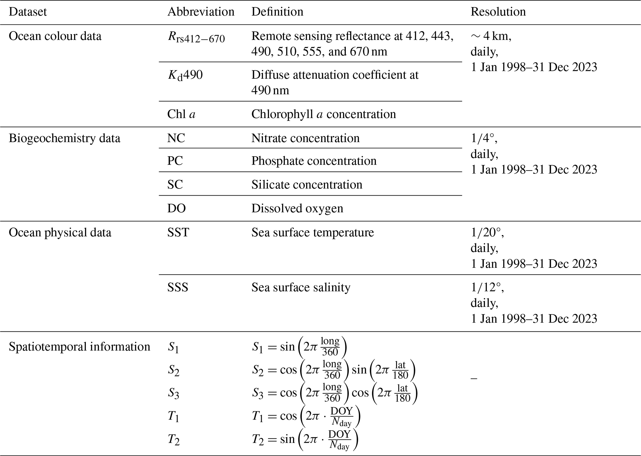
2.2.3 Ocean physics, biogeochemistry data, and spatiotemporal information

Incorporation of physical oceanographic data, including sea surface temperature (SST) and sea surface salinity (SSS), alongside biogeochemical data (Table 2) was performed. These data are provided by the Copernicus Marine Data Store (https://data.marine.copernicus.eu/products, last access: 21 October 2024). The SST data are sourced from the ESA SST CCI (Climate Change Initiative) and C3S (Copernicus Climate Change Service) global Sea Surface Temperature Reprocessed product (https://doi.org/10.48670/moi-00169, Copernicus Marine Service, 2023a), covering the period from January 1998 to October 2022, and the Global Ocean OSTIA Sea Surface Temperature and Sea Ice Analysis (https://doi.org/10.48670/moi-00165, Copernicus Marine Service, 2023b), covering the period from November 2022 to December 2023. The SSS data are obtained from the Global Ocean Physics Reanalysis (https://doi.org/10.48670/moi-00021, Copernicus Marine Service, 2023c). Biogeochemical data include the nitrate concentration (NC), phosphate concentration (PC), silicate concentration (SC), and dissolved oxygen (DO). These variables are critical for understanding the nutrient dynamics in marine ecosystems, which are fundamental factors influencing phytoplankton growth and distribution. The data for these biogeochemical variables are sourced from the multiyear Global Ocean Biogeochemistry Hindcast products (https://doi.org/10.48670/moi-00019, Copernicus Marine Service, 2024). All data undergo the preprocessing steps outlined in the following. First, all data are resampled to a 4 km resolution using the pysample library (https://doi.org/10.5281/zenodo.3372769, Hoese et al., 2024). The inverse distance weighting (IDW) method was employed for spatial interpolation. IDW identifies all available pixels around a target pixel based on a search radius of eight pixels, and the weights of the identified available pixels are then calculated by the reciprocal of the square of the distance between the target pixel and the available pixels. This resampling process may lead to missing pixels, which are then filled using the nearest-neighbour method. Second, data are standardized. For R_rs, L2-norm normalization is performed, meaning each band (i.e. R_rs412, R_rs443, R_rs490, R_rs510, R_rs560, and R_rs665) is divided by the square root of the sum of squares of all bands. For Chl a and K_d490, as well as NC, PC, SC, DO, SST, and SSS, standardization is carried out using the StandardScaler function from the scikit-learn library (https://scikit-learn.org/, last access: 21 October 2024).

Incorporating spatial–temporal encoding into models is an effective strategy to enhance prediction accuracy, allowing for better capture of complex spatial–temporal interactions within the data (Yang et al., 2022; Wei et al., 2023). The spatial term is characterized in Euclidean space using three spherical coordinates $[S_{\mathrm{1}},S_{\mathrm{2}},S_{\mathrm{3}}]$ to reflect autocorrelation and spatial differences. These coordinates represent a point's position in three-dimensional space, calculated as follows: (1) S₂ describes the component in the east–west direction, calculated by longitude, with the formula $S_{\mathrm{1}}=\sin \left(\mathrm{2}\mathit{\pi }\frac{\text{long}}{\mathrm{360}}\right)$; (2) S₂ combines longitude and latitude to provide the position in the north–south direction and the vertical distance from the Equator, calculated as $S_{\mathrm{2}}=\cos \left(\mathrm{2}\mathit{\pi }\frac{\text{long}}{\mathrm{360}}\right)\sin \left(\mathrm{2}\mathit{\pi }\frac{\text{lat}}{\mathrm{180}}\right)$; (3) S₃ represents the straight-line distance from the centre of the Earth to the point, calculated as $S_{\mathrm{3}}=\cos \left(\mathrm{2}\mathit{\pi }\frac{\text{long}}{\mathrm{360}}\right)\cos \left(\mathrm{2}\mathit{\pi }\frac{\text{lat}}{\mathrm{180}}\right)$. Furthermore, the temporal term ($T\sim [T_{\mathrm{1}},T_{\mathrm{2}}]$) is represented by two sine and cosine functions of the day of the year (DOY), enabling the capture of both daily variations and seasonal patterns in the PFT. Here, $T_{\mathrm{1}}=\cos \left(\mathrm{2}\mathit{\pi }\cdot \frac{\text{DOY}}{N_{\mathrm{day}}}\right)$ and $T_{\mathrm{2}}=\sin \left(\mathrm{2}\mathit{\pi }\cdot \frac{\text{DOY}}{N_{\mathrm{day}}}\right)$, where N_day is the total number of days in the corresponding year.

2.3 Spatial–temporal–ecological ensemble model based on deep learning

In the previous research by Zhang et al. (2023), the focus was primarily on the generation of monthly PFT Chl a data products, for which the STEE (spatial–temporal–ecological ensemble) model was developed. The STEE model integrates three complex machine learning methods aimed at achieving high prediction accuracy. However, when the present study shifted from monthly to daily predictions, the computational demand increased significantly, turning the processing speed of the model into a critical bottleneck. Additionally, although the previous STEE model is capable of making high-precision predictions, it does not provide an uncertainty assessment for these predictions, which is a drawback in many ecological applications. To address these challenges, the present study further developed the STEE-DL (spatial–temporal–ecological ensemble model based on deep learning).

2.3.1 Network architecture

Ensemble learning has emerged as a powerful approach to enhancing prediction performance by combining the outputs of multiple models. STEE-DL models that use deep ensemble learning combine the advantages of deep learning with those of ensemble learning to achieve better generalization. The STEE-DL model framework introduces an ensemble consisting of N residual neural networks as its components. Residual neural networks are known for their shortcut connections, which help in maintaining a smooth flow of gradients during the learning process. To ensure efficiency, each component model is built with two residual blocks designed to reduce computational demands while preserving the effectiveness of a deep network. These blocks comprise a fully connected layer, a rectified linear unit (ReLU) activation function, and a shortcut connection for uninterrupted information transmission. In this model, the input layer receives 19 feature variables, which are then reduced to 16 after the first residual block. Subsequently, the second residual block further reduces the number of features to 10. Finally, a fully connected layer maps these features to an output value for predicting the target variable. Chau et al. (2022) has shown that ensemble stability improves significantly when the number of component models, N, exceeds 50, but the marginal gains in reducing standard error diminish after reaching 100 models. Therefore, aiming for a balance between accuracy and computational efficiency, we have chosen an ensemble size of N=100. Based on this architecture, we have implemented the STEE-DL models using PyTorch (https://pytorch.org/, last access: 21 October 2024).

2.3.2 Model ensemble and uncertainty

Each ResNet within the ensemble focuses on different subsets and features of the training data, The mean (μ) of the outputs from the 100 independent models is considered the optimal estimation of the target variable.

$$\begin{array}{}\text{(2)}& {\mathit{\mu }}_{\mathrm{pft}}=\sum _{i=\mathrm{1}}^{i=\mathrm{100}}{\mathrm{PFT}}_{\mathrm{estimated}\left(i\right)}/\mathrm{100}\end{array}$$

The variability among ensemble model outputs, quantified by the standard deviation (σ) of the 100 independent models, provides a measure of uncertainty in predictions (Chau et al., 2022). This uncertainty reflects the variability in predictions due to differences in training sets, initializations, and learning dynamics. A higher standard deviation indicates greater disagreement among models, suggesting lower confidence in the prediction. It should be noted that all computations of the uncertainties in this study were conducted on log10-transformed data, which follows conventional practice in the field of ocean colour research (Xi et al., 2021).

$$\begin{array}{}\text{(3)}& \mathit{\sigma }=\sqrt{\sum _{i=\mathrm{1}}^{i=\mathrm{100}}{\left({\mathrm{PFT}}_{\mathrm{estimated}\left(i\right)}-{\mathit{\mu }}_{\mathrm{pft}}\right)}^{\mathrm{2}}/\mathrm{100}}\end{array}$$

This approach differs from statistical methods based on error propagation, which evaluate prediction uncertainty by analysing input data uncertainties (e.g. measurement errors) and their transmission through the model to the outputs. Such methods require a clear understanding of input error distributions and typically assume these errors are independent. Given the STEE-DL model's reliance on diverse marine and in situ HPLC data of varying levels of quality control, accurately applying error propagation for uncertainty measurement is challenging. Our ensemble-based approach primarily addresses model uncertainty but also indirectly reveals data uncertainties by demonstrating how predictions respond to variations in representation and data subsets.

2.3.3 Training procedure

To compile the training dataset, we align in situ HPLC data with reconstructed OC-CCI and environmental data, both spatially and temporally. This alignment projects the data onto a 4 km grid according to the latitude, longitude, and date of the HPLC measurements. In cases in which several HPLC measurements are located within the same 4 km grid cell, we average these measurements to consolidate corresponding predictor variables. Figure S1 in the Supplement presents the histograms of the Chl a concentrations of the eight PFTs on a log10 scale.

The STEE-DL model utilizes a Monte Carlo and bootstrapping ensemble learning approach to boost model stability and predictive accuracy. By resampling, it randomly selects two-thirds of the total dataset as the training set for each iteration, repeating this procedure 100 times. This method is designed to create a varied collection of models by multiple rounds of sampling, significantly improving the model's ability to generalize. This reduces the model's reliance on specific data distributions, thereby increasing both the accuracy and the robustness of its predictions.

Throughout the training phase, the model optimization relies on the Adam optimizer, complemented by L1 regularization to promote sparsity within the model and prevent overfitting. Gradient clipping is applied to manage potential issues with exploding gradients, thereby ensuring a more stable training process. An exponential moving average (EMA) strategy is employed to stabilize the model weights by averaging them over time, which helps to minimize variations and secure consistent performance from the final model.

To circumvent the issue of the model predicting unreasonably high values during training, we have crafted a specialized loss function. This function incorporates the traditional mean-squared error (MSE) while imposing extra penalties on predictions that surpass set thresholds. Not only does this effectively prevent the model from making unrealistic predictions, but it also guides the model towards more-accurate parameter adjustments, assuring that its predictions stay within feasible limits.

2.4 Evaluation strategies

To comprehensively test the accuracy and robustness of the model, the evaluation of the STEE-DL model comprises two parts: first, the model performance is validated using a 5-fold cross-validation method in three different ways; second, the evaluation is based on a tripartite-matching analysis algorithm.

2.4.1 Cross-validation approach

Cross validation (CV) is a commonly used method for analysing model performance, allowing for a comprehensive assessment of a model's accuracy, stability, and generalization. This study implements three types of CV to deeply evaluate the model's multifaceted performance: random 5-fold CV, time-block 5-fold CV, and spatial-block 5-fold CV. Specifically, the methods are as follows:

1. Standard 5-fold cross-validation. This method randomly divides all data into five equal-sized subsets. In each round of validation, one subset is selected as the test set, while the remaining four subsets serve as the training set, ensuring that each data point is used as test data. This method primarily evaluates the model's performance and generalization on the entire dataset.

2. Time-block 5-fold cross-validation. Data are divided into five consecutive time periods in chronological order. In each iteration, data from one time period are chosen as the test set, with the data from the remaining periods serving as the training set (as shown in Fig. 5). This method takes into account the continuity and dependency of time series, helping to evaluate the model's ability to capture time trends and seasonal variations.

3. Spatial-block 5-fold cross-validation. This method is similar to time-block cross-validation, but data are divided based on spatial location. A hexagonal grid was created at 20° horizontal and vertical intervals, and regions without sampling points were removed for hexagonal regions. In each round, data from one geographical block are left out as the test set, while data from other blocks are used for training (as shown in Fig. 6). This method prevents potential data leakage due to spatial autocorrelation and helps to assess the model's spatial prediction capability and its generalization across different geographical locations.

Figure 5 Temporal-block CV procedure.

The coefficient of determination (R²), root-mean-square error (RMSE), mean absolute error (MAE), and symmetric mean absolute percentage error (sMAPE) were utilized to quantify the performance of the model, according to the following expressions:

$$\begin{array}{}\text{(4)}& {\displaystyle }{R}^{\mathrm{2}}=\mathrm{1}-{\displaystyle \frac{{\sum }_{i=\mathrm{1}}^N{\left[p_i-{\widehat{p}}_i\right]}^{\mathrm{2}}}{{\sum }_{i=\mathrm{1}}^n{\left[p_i-\overline{p}\right]}^{\mathrm{2}}}},\text{(5)}& {\displaystyle }\mathrm{RMSE}={\left[{\displaystyle \frac{\mathrm{1}}{N}}\sum _{i=\mathrm{1}}^N{\left(p_i-{\widehat{p}}_i\right)}^{\mathrm{2}}\right]}^{\mathrm{1}/\mathrm{2}},\text{(6)}& {\displaystyle }\mathrm{MAE}={\displaystyle \frac{\mathrm{1}}{N}}\sum _{i=\mathrm{1}}^N\left|p_i-{\widehat{p}}_i\right|,\text{(7)}& {\displaystyle }\mathrm{sMAPE}={\displaystyle \frac{\mathrm{100}}{N}}{\sum }_{i=\mathrm{1}}^N{\displaystyle \frac{\mathrm{|}{\widehat{p}}_i-p_i\mathrm{|}}{({\widehat{p}}_i-p_i)/\mathrm{2}}}.\end{array}$$

Here, p_i and ${\widehat{p}}_i$ are the log10-scaled observed and estimated values of each PFT for sample i, respectively; N is the number of observations; and $\overline{p}$ is the log10-scaled mean of the observed values.

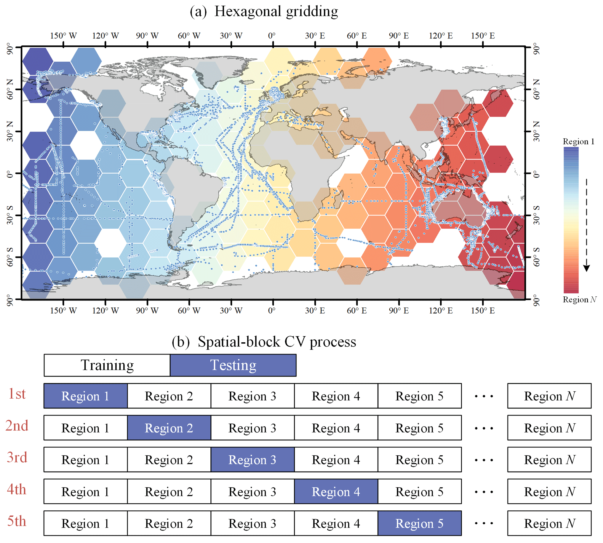
Figure 6 Spatial-block CV procedure.

2.4.2 Triple-collocation analysis

The triple-collocation analysis (TCA) method was also utilized for a global evaluation of the AIGD-PFT data product. TCA is a technique that allows for the assessment and quantification of error characteristics in three independent data sources without relying on reference data pre-assumed to be “true” (McColl et al., 2014). This method has been widely adopted in the uncertainty evaluation of remote sensing products across various fields, including soil moisture (Kim et al., 2023), sea surface salinity (Hoareau et al., 2018), and sea surface temperature (Saleh and Al-Anzi, 2021).

For error statistics based on TCA, we selected the fractional mean-squared error (fMSE) and the squared correlation coefficient. These metrics offer direct insights into data precision and accuracy. The fMSE, in particular, is beneficial because it quantifies the relative error in a product, scaling from 0 to 1, where a lower value indicates higher precision. The fMSE is calculated as follows:

$$\begin{array}{}\text{(8)}& {\text{fMSE}}_i={\displaystyle \frac{{\mathit{\sigma }}_{{\mathit{\epsilon }}_i}^{\mathrm{2}}}{{\mathit{\sigma }}_i^{\mathrm{2}}}}={\displaystyle \frac{{\mathit{\sigma }}_{{\mathit{\epsilon }}_i}^{\mathrm{2}}}{{\mathit{\beta }}_i^{\mathrm{2}}{\mathit{\sigma }}_{\mathrm{\Theta }}^{\mathrm{2}}+{\mathit{\sigma }}_{{\mathit{\epsilon }}_i}^{\mathrm{2}}}}={\displaystyle \frac{\mathrm{1}}{\mathrm{1}+{\text{SNR}}_i}}.\end{array}$$

Here, $i={\mathit{\alpha }}_i+{\mathit{\beta }}_i\mathrm{\Theta }+{\mathit{\epsilon }}_i$ corresponds to three spatially and temporally collocated datasets $\left[X,Y,Z\right]$; ${\mathit{\sigma }}_{{\mathit{\epsilon }}_i}^{\mathrm{2}}$ is the TCA-based error variance of an individual product; β_i and α_i represents the scaling factor and systematic additive biases between the unknown true signal Θ and the datasets i, respectively; ${\mathit{\sigma }}_i^{\mathrm{2}}$ is the variance of the individual data; ${\mathit{\sigma }}_{\mathrm{\Theta }}^{\mathrm{2}}$ is the variance of the true signal; and SNR is the signal-to-noise ratio. An fMSE value below 0.5 suggests that the true signal is a more significant component of the data than the estimation noise, indicating a precise product. Similarly, the squared correlation coefficient ($R_i^{\mathrm{2}}$) is defined as follows:

$$\begin{array}{}\text{(9)}& R_i^{\mathrm{2}}={\displaystyle \frac{{\mathit{\beta }}_i^{\mathrm{2}}{\mathit{\sigma }}_{\mathrm{\Theta }}^{\mathrm{2}}}{{\mathit{\beta }}_i^{\mathrm{2}}{\mathit{\sigma }}_{\mathrm{\Theta }}^{\mathrm{2}}+{\mathit{\sigma }}_{{\mathit{\epsilon }}_i}^{\mathrm{2}}}}={\displaystyle \frac{{\text{SNR}}_i}{\mathrm{1}+{\text{SNR}}_i}}.\end{array}$$

The foundational assumptions of TCA are important for its application (Kim et al., 2023). These assumptions are as follows: (1) a linear relationship exists between each dataset and the true signal, (2) the errors among the datasets are orthogonal, and (3) there is no correlation among the errors of different datasets. These principles ensure the robustness of the TCA method with respect to providing an unbiased error and quality assessment of products.

Several other PFT Chl a data products were introduced and organized into triads for TCA analysis. First, the SynSenPFT (https://doi.org/10.1594/PANGAEA.875873, Losa et al., 2017b) and NOBM-daily products were obtained, forming daily product triplets. Both SynSenPFT and NOBM-daily contain three PFTs – diatoms, cyanobacteria (prokaryotes), and coccolithophores (the main contributing PFT to haptophytes). TCA evaluations were conducted separately for these three PFTs. The TCA calculation process selected overlapping time periods of SynSenPFT, NOBM-daily, and the proposed AIGD-PFT data products, from 1 August 2002 to 31 March 2012, totalling 3515 d. All three products were resampled to a 1° resolution. Similarly, we also obtained EOF-PFT data (https://doi.org/10.48670/moi-00281, Copernicus Marine Service, 2023d) and the NOBM-monthly product to form monthly triplets, again conducting TCA assessments for diatoms, prokaryotes, and haptophytes. Before evaluation, the AIGD-PFT data products were merged on a monthly basis and resampled to a 1° resolution along with EOF-PFT and NOBM-monthly. The temporal span of monthly TCA triplet products was from January 2003 to December 2017, totalling 180 months. NOBM's daily and monthly data were all obtained from the NASA Giovanni website (https://giovanni.gsfc.nasa.gov/, last access: 21 October 2024). We additionally employed RECCAP2-ocean (Regional Carbon Cycle Assessment and Processes) regions for regional TCA statistics, as shown in Fig. 7.

Figure 7 Map of RECCAP2-ocean (Regional Carbon Cycle Assessment and Processes) regions (https://reccap2-ocean.github.io/regions/, last access: 21 October 2024; Canadell et al., 2011), including the Arctic (Ar), subtropical Atlantic (StA), equatorial Atlantic (EA), South Atlantic (SA), subtropical Pacific (StP), equatorial Pacific (EP), South Pacific (SP), Indian Ocean (IO), and Southern Ocean (SO).

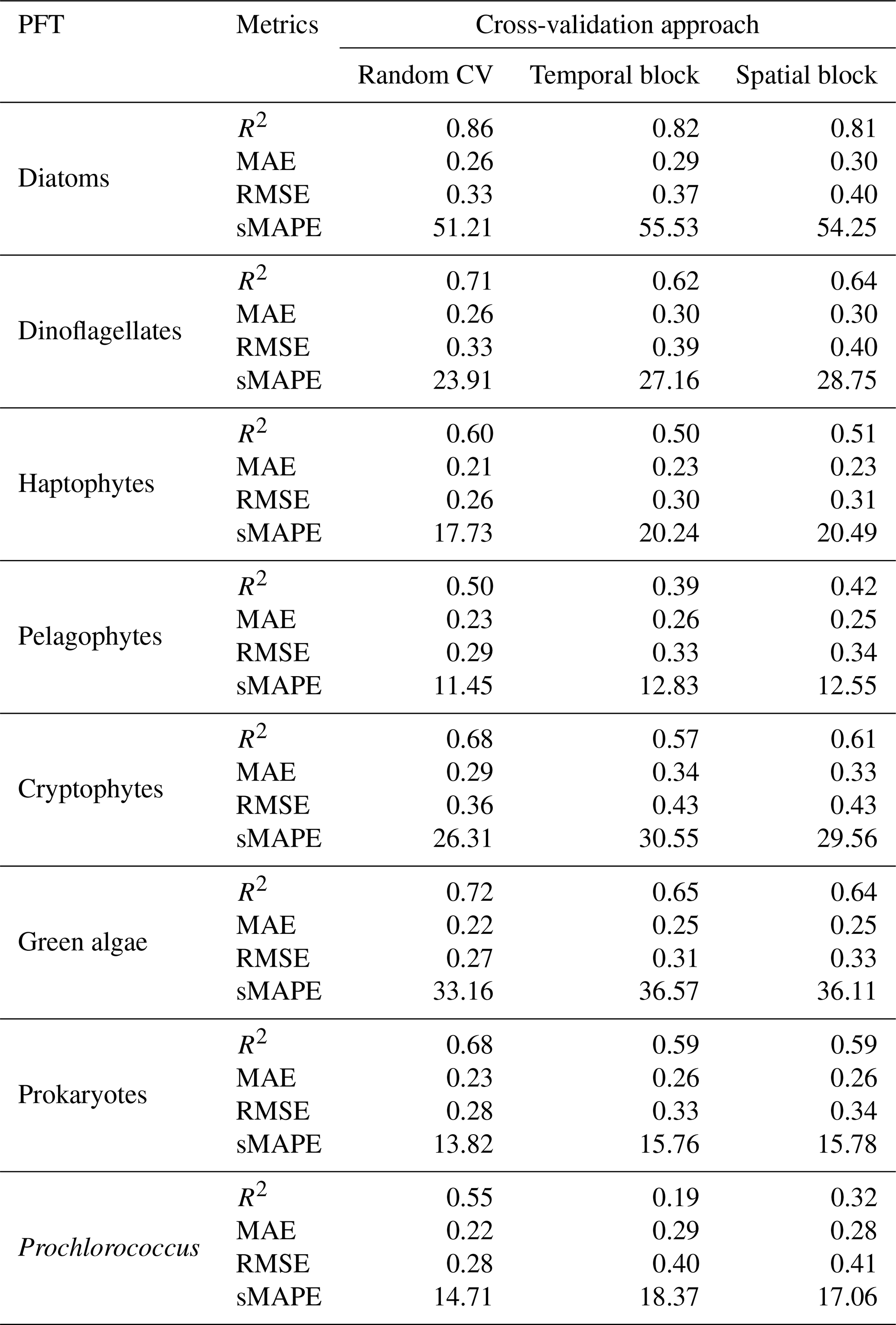
Table 3 Model performance metrics (R², MAE, RMSE, and sMAPE) based on a random, temporal-block, and spatial-block 5-fold CV procedure.

3 Results

3.1 Model verification

3.1.1 The three CV methods

To comprehensively assess the performance of the proposed STEE-DL model, three 5-fold cross-validation (CV) methods were implemented: random, temporal-block, and spatial-block CV. The results are shown in Table 3. The random CV analysis revealed generally high prediction accuracy across all eight PFTs, as visualized by the scatter plot in Fig. 8. Diatoms exhibited the best performance, achieving an R² value of 0.8. This confirms the STEE-DL model's strong capability with respect to diatom prediction. Conversely, pelagophytes displayed the weakest performance, reflected by an R² value of just 0.5. Further examination using the probability distribution histograms and cumulative distribution function (CDF) curves of predicted vs. actual values revealed a good alignment, indicating the model's overall ability to accurately mimic observed data distributions. However, a notable limitation observed was the STEE-DL model's tendency towards overestimating lower values and underestimating higher values. This suggests a bias towards predicting smoother values, potentially resulting in less-accurate predictions for extreme high or low actual values.

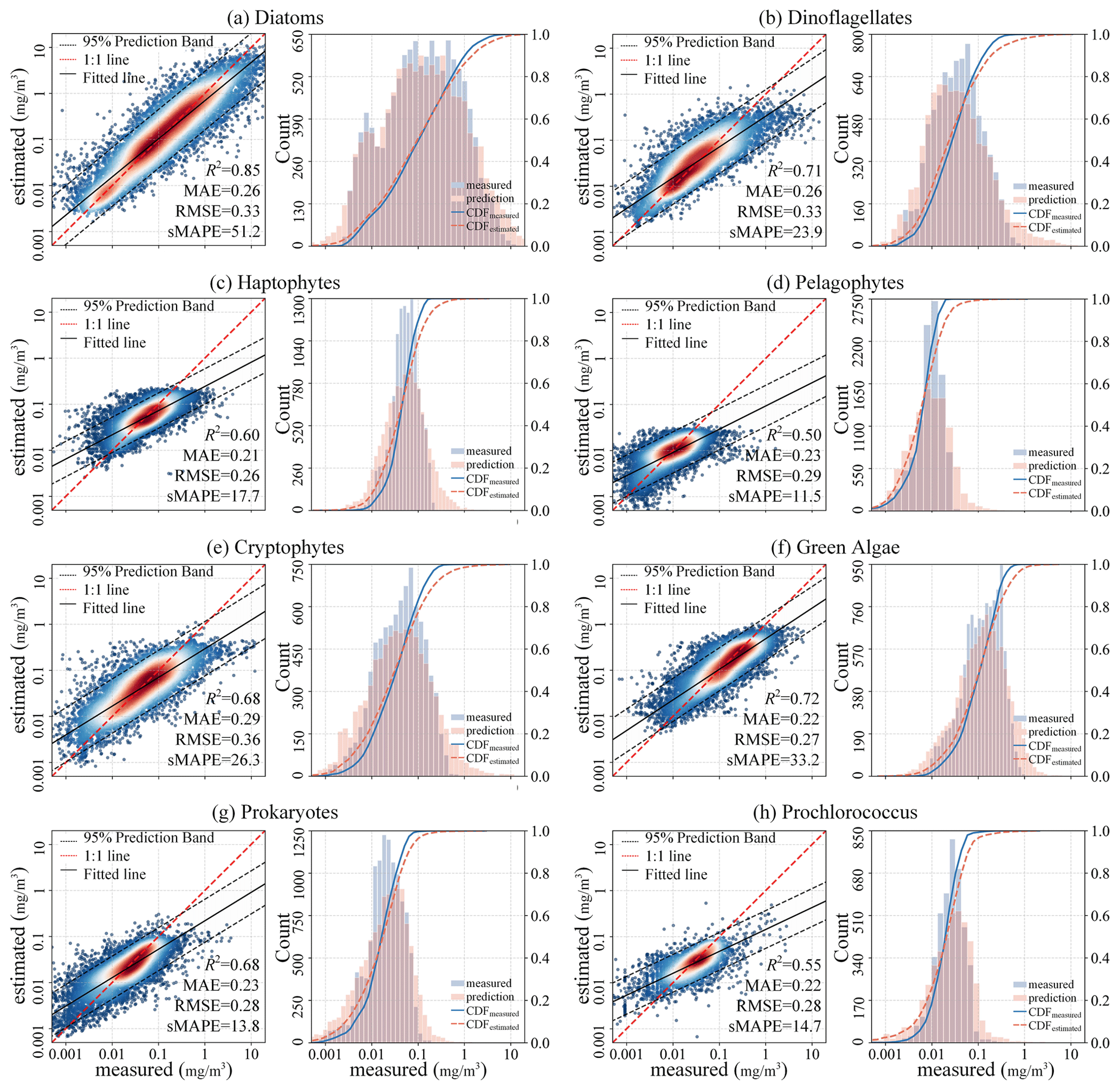
Figure 8 Scatter diagrams, probability distribution histograms, and cumulative distribution function (CDF) curves (based on a random 5-fold CV procedure) of the predicted vs. measured Chl a concentrations of eight PFTs.

By comparing the model performance under three different CV strategies, we delved further into the STEE-DL model's generalization abilities in terms of time and space. Figure 9 reveals that the STEE-DL model's accuracy decreases when using temporal and spatial cross-validation compared with standard random cross-validation. Notably, the predictive accuracy for diatoms was minimally affected by the different validation strategies, with R² values remaining above 0.8 for all three methods. This demonstrates the model's robust generalization capability in both the temporal and spatial aspects. Except for Prochlorococcus, the decrease in accuracy was modest for other PFTs in spatial cross-validation (with about a 0.1 decrease in the R² and a 0.5 increase in the MAE), suggesting that the STEE-DL model is relatively robust and can accurately estimate regions lacking in situ observational data. Compared with spatial validation, there was a slight decrease in accuracy for temporal cross-validation, although it still maintained a good level. Except for a significant drop in temporal generalization for Prochlorococcus, the temporal cross-validation accuracy for other PFTs remained favourable.

Figure 9 Comparison of the results obtained using different CV methods, including random CV, spatial-block CV, and temporal-block CV. Blue indicates variations in the R² for the three CV strategies, while red represents changes in MAE.

During the training process of the STEE-DL model, two types of training data were utilized: “original match” training data and “reconstructed match” training data. The original match training data refer to data successfully matched directly from the in situ HPLC database and the OC-CCI original data, whereas reconstructed match training data refer to matched data obtained after completing the missing parts of OC-CCI data using the DCT-PLS technique. By comparing the model's prediction accuracy on these two types of data, we can assess not only the STEE-DL model's adaptability to changes in data completeness but also verify the effectiveness and accuracy of the DCT-PLS technique with respect to reconstructing missing ocean colour data. If the STEE-DL model's performance on the reconstructed match data is similar to its performance on the original match data, it not only indicates that the DCT-PLS method is effective and reasonable for reconstructing ocean colour data but also confirms that the STEE-DL model can provide reliable PFT predictions under varying data quality and completeness conditions.

We calculated the R² between predicted and actual values for both original and reconstructed pixels using the three cross-validation methods (Fig. 10). Except for a significant difference in performance for Prochlorococcus, the accuracy of reconstructed pixels was generally consistent with that of the original pixels, demonstrating good performance. This indicates that the reconstructed pixels did not degrade model performance, thus confirming both the high congruency of our data reconstruction method with actual conditions and the robustness of the STEE-DL model.

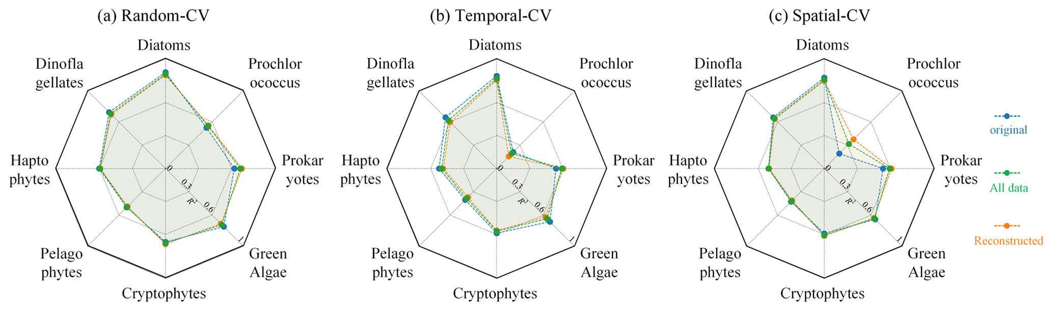
Figure 10 Model performance comparison for original pixels (dashed blue line), reconstructed pixels (dashed orange line), and all pixels (solid orange line) using (a) random CV, (b) temporal CV, and (c) spatial CV.

3.1.2 Long-time-series observations

The effectiveness of the proposed STEE-DL model was validated using data from six independent long-term observation sites. The results, as shown in the Fig. 11, display the correlation coefficients between predicted and actual values at these six sites. The STEE-DL model demonstrated varying degrees of predictive capability across different sites and PFTs. Firstly, the model achieved high prediction accuracy for key functional types, such as diatoms, dinoflagellates, and green algae, with significant advantages at certain sites: for instance, at sites 4 and 5, the prediction correlation coefficients for diatoms were as high as 0.90 and 0.88, respectively. Site 5 exhibited high correlations for dinoflagellates and green algae predictions, reaching 0.69 and 0.83, respectively, highlighting the model's ability to accurately capture the dynamics of these major functional types. However, it is noteworthy that predictions for certain functional types showed considerable fluctuations at specific sites. For example, site 3 had a prediction correlation coefficient of 0.90 for pelagophytes but a relatively lower coefficient of 0.48 for dinoflagellates. In terms of functional types like prokaryotes and Prochlorococcus, the model's predictions were generally more balanced, with site 2 showing a high correlation coefficient of 0.80 for Prochlorococcus. Overall, despite some fluctuations and differences, these results emphasize the STEE-DL model's capability to capture the temporal trends in different PFTs with relative accuracy.

Figure 11 STEE-DL model performance at six independent time-series stations, showing the correlation coefficient (bar chart) and number of successfully matched pixels (dashed blue line).

3.2 The gap-free PFT data product and uncertainties

Following the validation of the STEE-DL model, it was retrained with the entirety of the data available, enabling the generation of a long-time-series spatiotemporally continuous AIGD-PFT data product for the period from 1998 to 2023. An example comparison from this dataset, depicted in Fig. 12 for 10 March 2020, demonstrates the results of the AIGD-PFT. Notably, while nearly half of the original OC-CCI data contained missing values (as shown in Fig. 12a), our reconstructed dataset has achieved spatial completeness with good continuity. Within this dataset, the distribution patterns of the eight PFTs showed significant variability. For example, diatoms were primarily found in the oceanic regions of the middle to high latitudes (30–60°), thriving in nutrient-rich, cold waters, and areas affected by terrestrial runoff. Dinoflagellates, with a distribution pattern similar to diatoms, were mostly present in the nutrient-rich upwelling zones of high latitudes and nearshore areas, although their content was relatively lower. Prokaryotes were noted for maintaining higher concentrations in the nutrient-poor, sunlight-abundant waters of tropical and subtropical regions (0–30°), with a significant decrease in biomass at higher latitudes, a characteristic closely resembling that of Prochlorococcus. Haptophytes and green algae were observed more frequently in the subtropical regions of the Pacific, Atlantic, and the Southern Ocean, reaching into middle and high latitudes. In contrast, pelagophytes and cryptophytes were found to be more prevalent in tropical and subtropical regions, showing lower concentrations in areas of lower latitude. Additionally, the yearly mean maps for 2020 are provided in Fig. S2, showing the distribution pattern of global ocean PFTs throughout the year.

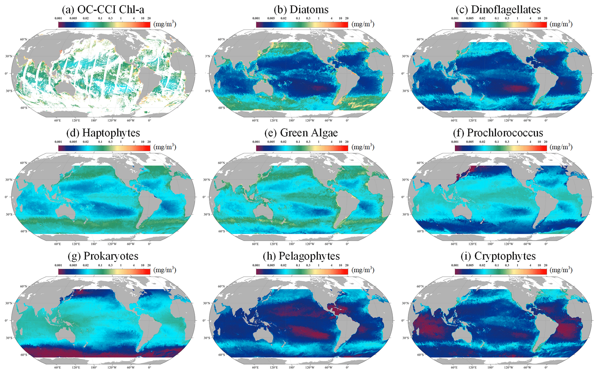
Figure 12 The global distribution (10 March 2020) of the Chl a concentration for (a) original OC-CCI, (b) diatoms, (c) dinoflagellates, (d) haptophytes, (e) green algae, (f) Prochlorococcus, (g) prokaryotes, (h) pelagophytes, and (i) cryptophytes. The grey areas represent land.

Figure 13 delineates the corresponding uncertainties. Overall, the uncertainty is relatively low in the open ocean, suggesting that the model performs with a high degree of confidence. However, in coastal regions, such as the East China Sea and the Amazon River estuary, uncertainties escalate. This increase likely results from the complex coastal processes and land–sea interactions prevalent in these areas, which can significantly influence the distribution and concentrations of PFTs, thereby challenging the model's predictive accuracy. Despite the coastal uncertainties, Fig. 13 also reveals that AIGD-PFT maintains globally low uncertainty levels (below 0.1) for diatoms, dinoflagellates, haptophytes, and prokaryotes, highlighting the model's overall stability and reliability. Additionally, Prochlorococcus exhibits higher uncertainties in the Southern Ocean, while cryptophytes show increased uncertainty in the equatorial Pacific. The reasons for this specific pattern require further investigation. Additionally, Fig. S3 illustrates the global distribution of uncertainties on 10 July 2020.

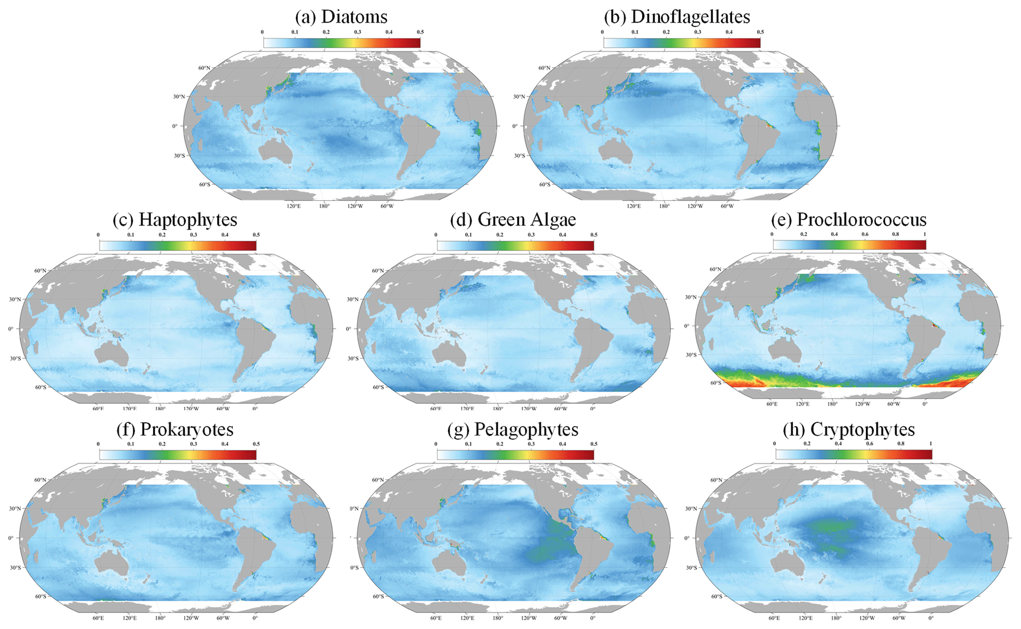
Figure 13 The global distribution (10 March 2020) of the uncertainties for (a) diatoms, (b) dinoflagellates, (c) haptophytes, (d) green algae, (e) Prochlorococcus, (f) prokaryotes, (g) pelagophytes, and (h) cryptophytes.

Further, Fig. 14 illustrates the AIGD-PFT's ability to capture dynamic coastal processes, such as estuary runoff and coastal circulations, through time-series images of the diatom distribution in the Amazon River estuary (Fig. 11a) and the Gulf of Mexico (Fig. 11b). The high diatom concentrations near the Amazon River estuary, as shown in Fig. 6a, were correlated with the area's rich nutrient influx, also capturing the influence of the North Brazil Current (NBC) along the Brazilian coastline on diatom dispersion. Figure 6b demonstrates the AIGD-PFT's efficacy with respect to depicting the characteristics dominated by circulation and associated eddies in the Gulf of Mexico.

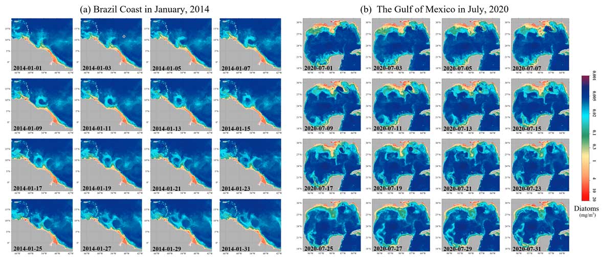
Figure 14 Gap-free diatom Chl a concentrations for the (a) Brazilian coast in January 2014 and (b) Gulf of Mexico in July 2020.

3.3 TCA-based assessment

As depicted in Fig. 15, we conducted a TCA on three daily PFT data products: AIGD-PFT, SynSenPFT, and NOBM-daily. Figure 15a presents the statistical analysis results of correlation coefficients (R) and mean-squared error (fMSE) at the global scale. Meanwhile, Fig. 15b, c, and d detail the comparative assessment results across different marine regions. Globally, the AIGD-PFT data product outperforms the other two, demonstrating the highest median correlation values with actual conditions for diatoms (0.81), haptophytes (0.80), and prokaryotes (0.72), respectively. The AIGD-PFT data product also has the lowest fMSE values for all three PFTs, confirming its superiority, with values of 0.35, 0.35, and 0.48, respectively. Comparatively, the SynSenPFT product underperforms relative to NOBM-daily product with respect to estimating diatoms and prokaryotes, yet it excels at estimating haptophytes.

The regional analysis (Fig. 15b, c, and d) reveals variation in the R and fMSE values across regions and PFTs. AIGD-PFT consistently outperforms in most regions with respect to diatom estimation, but it shows a slight increase in the fMSE in the equatorial Pacific, indicating a potential dip in estimation accuracy in this area. In contrast, SynSenPFT registers higher fMSE values for haptophyte estimation, particularly in the subtropical and southern Pacific regions. NOBM-PFT, on the other hand, tends to have a lower correlation for haptophyte estimation across regions, with a notable deficiency near the equatorial Pacific. Additionally, SynSenPFT demonstrates higher global fMSE values for prokaryotes compared with the other datasets, and NOBM-PFT significantly underperforms with respect to prokaryotes estimation in the Southern Ocean.

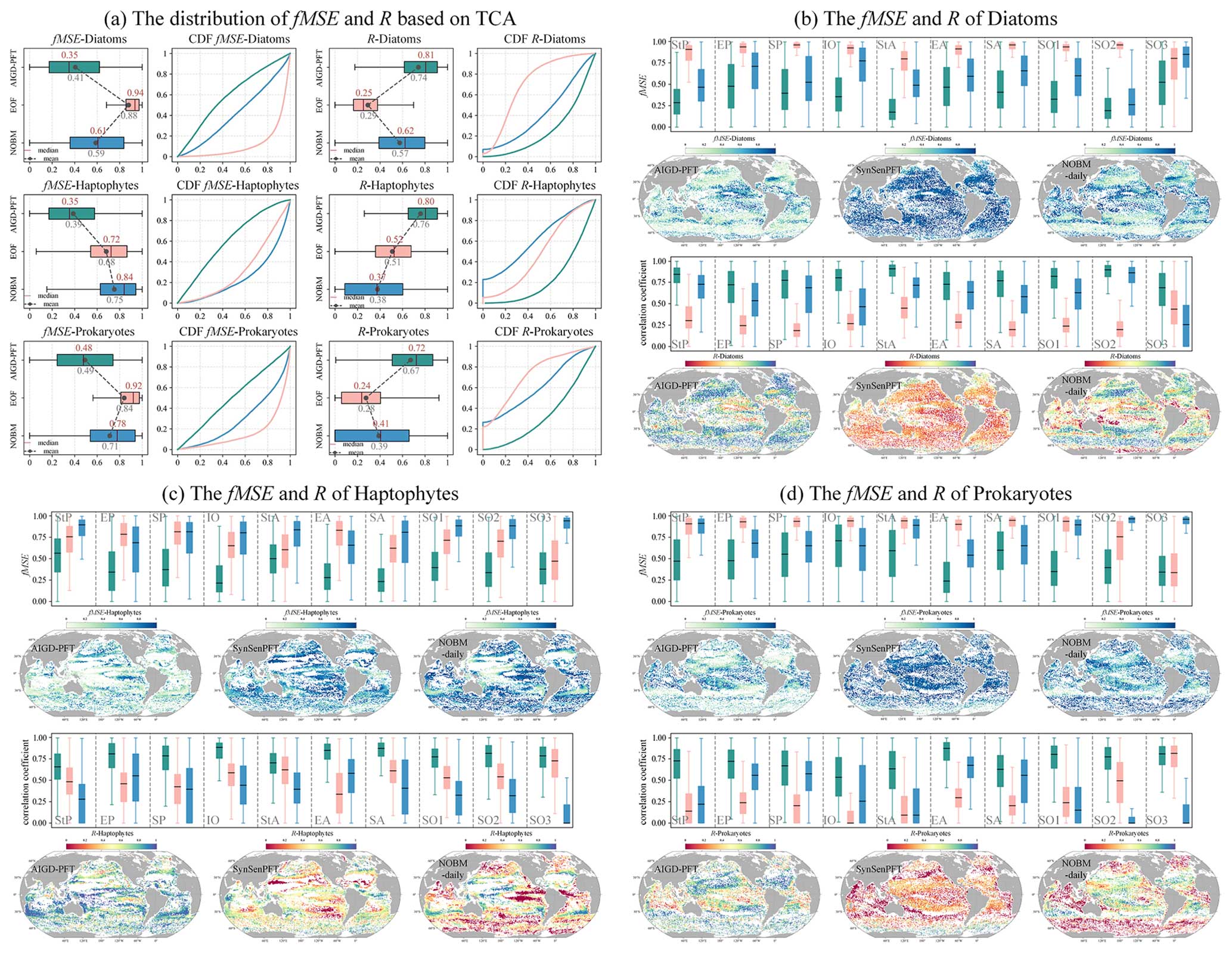
Figure 15 TCA result of the three daily products (AIGD-PFT, SynSenPFT, and NOBM-daily).

We now further extend our analysis to monthly products (AIGD-PFT, EOF-PFT, and NOBM-monthly). As detailed in Fig. 16, we observed that AIGD-PFT and EOF-PFT exhibit closely matched performance for diatoms, with median R values of 0.87 and 0.86 and fMSE values of 0.24 and 0.25, respectively. Their CDF curves nearly align perfectly. Although global assessments for diatoms are consistent, regional discrepancies exist. For instance, the AIGD-PFT and EOF-PFT data products perform similarly in the subtropical Pacific and the Indian Ocean, but the AIGD-PFT data product achieves a superior correlation in the equatorial Pacific, Southern Ocean, and subtropical Atlantic. Conversely, the EOF-PFT product performs better in the South Pacific and equatorial Atlantic. In summary, for haptophytes and prokaryotes, both global and regional assessments suggest that the AIGD-PFT data product is the most effective dataset, offering the lowest median fMSE and highest median R values. It stands out not only on a global scale but also in most regional evaluations, confirming its overall superiority among the comparative datasets.

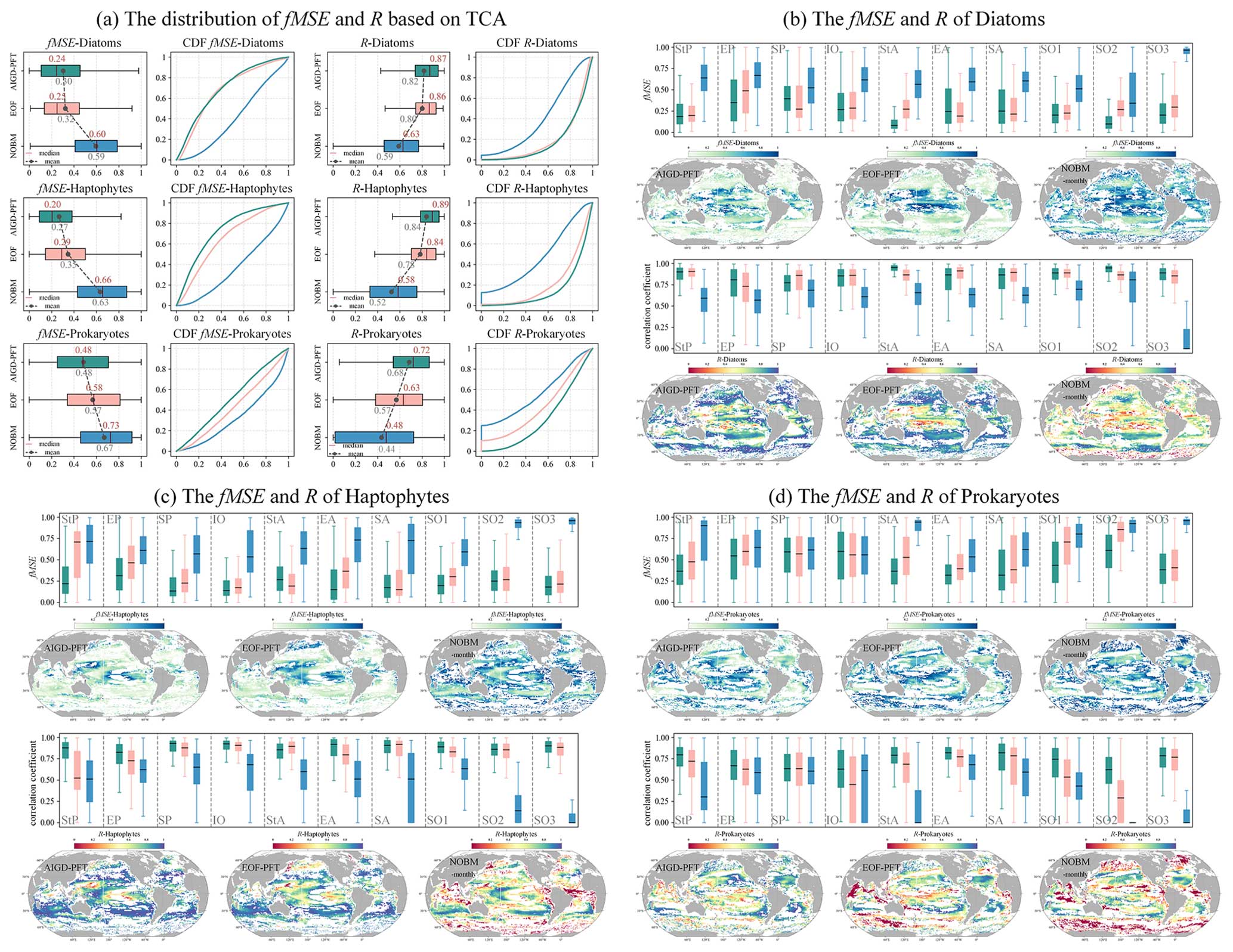
Figure 16 TCA result of the three monthly products (AIGD-PFT, EOF-PFT, and NOBM-monthly).

4 Discussion

Phytoplankton serve as the foundation of marine food chains. Comprehensive monitoring and inversion of the spatiotemporal distribution patterns of PFTs are crucial for a deeper understanding of marine ecosystem functions, predicting and mitigating climate change, and other aspects. Amidst increasing human reliance on marine resources, maintaining the sustainability of fisheries and ensuring the stability and health of marine, especially coastal, ecosystems have become particularly urgent. This necessitates higher-quality and more-detailed phytoplankton diversity data to assist decision-making. However, existing satellite PFT data products have significant shortcomings regarding inversion accuracy, spatiotemporal resolution, spatial coverage, and temporal span, limiting their application in climate and ocean management research. Therefore, enhancing the quality and coverage of PFT data, with higher temporal resolution, is essential to reveal the immediate impacts of environmental changes on the PFT distributions. Improved spatial coverage would enable more-accurate descriptions of local changes in marine ecosystems, providing more-precise data support for scientific management strategies. Additionally, extending the temporal span would enhance the accuracy of long-term trend analysis, thereby enabling a better understanding of the evolution of marine ecosystems. As environmental data continue to be updated, the STEE-DL model can be easily applied to future datasets, allowing for the continuous generation of PFTs, which will contribute to long-term global- or local-scale analyses.

Multisource marine big data exhibit complementary advantages in terms of spatial integrity and accuracy. By merging data on various environmental factors, we can produce improved PFT data products. In this study, we selected features including ocean colour data, biogeochemistry, temperature and salinity, and spatiotemporal information. Among these, ocean colour data, as a crucial predictor, were seamlessly reconstructed using a GPU-accelerated DCT-PLS algorithm, filling gaps caused by clouds, orbits, and other factors. Compared with traditional reconstruction algorithms, the DCT-PLS algorithm is faster and effectively addresses the issue of missing observational data, improving data utilization efficiency and monitoring continuity.

Further, by leveraging the powerful nonlinear modelling capabilities of deep learning, we enhanced the accuracy of PFT inversion. We developed a spatiotemporal ecological integration model based on deep learning, adapting the method proposed by Zhang et al. (2023) for reconstructing global PFTs from 1998 to 2023. The model, composed of 100 ResNet models, demonstrates strong nonlinear modelling capabilities and robustness. Using the Monte Carlo method, we utilized ensemble means and standard deviations as the optimal estimates and uncertainties, generating a temporally continuous global PFT data product covering the entire period and the corresponding uncertainty fields. The standard deviation reflects the variability in model predictions, indicating the consistency between model predictions, i.e. the level of uncertainty.

We also employed three cross-validation methods to comprehensively validate the accuracy. Standard 5-fold cross-validation focuses on the model's performance across the entire dataset, time-block 5-fold cross-validation assesses the model's handling of time series, and space-block 5-fold cross-validation concentrates on the model's ability to capture spatial distribution patterns. The results show that the STEE model generally exhibits good accuracy, demonstrating excellent performance and stability with respect to addressing temporal and spatial generalization issues. Notably, the model's high adaptability to reconstructed pixels highlights its potential for handling incomplete or inaccurate data, further proving the effectiveness of integrating ecological parameters and machine learning techniques. By applying the STEE model to all data from 1998 to 2023, we achieved accurate and robust monitoring of global high-resolution, spatiotemporally continuous PFT data products. The TCA algorithm was used to compare the AIGD-PFT data product with other products, showing that our estimation model achieved competitive overall accuracy.

Despite statistical and correlational analyses throughout the paper confirming the reasonable and reliable estimation of global PFTs by STEE-DL, some uncertainties and limitations still need to be addressed in further work. Firstly, in this study, all physical and biogeochemical data were resampled to match the 4 km (high) resolution, consistent with the OC-CCI product, primarily to ensure uniformity across datasets, as well as to maximize the use of existing data resources. However, resampling from a lower to a higher resolution can indeed alter the statistical properties of the data, potentially introducing inaccuracies. In future research, it is planned to incorporate more high-resolution data and to minimize the loss of information during the data-processing stage. Secondly, the variance obtained through ensemble learning mainly focuses on model prediction variability, but this does not fully capture or explain the actual product uncertainties. Real product uncertainties are broader, encompassing the incompleteness of actual measurements, uncertainties in predictors, and limitations in understanding the system. Exploring more comprehensive and precise uncertainty estimation methods to further enhance model reliability and applicability is necessary. It is also necessary to consider introducing a threshold based on existing ecological studies and global in situ data analysis, which will help filter out predictions in areas with high uncertainty. Additionally, the current STEE-DL model is solely based on statistical relationships and lacks the simulation of biological processes; therefore, it is unable to explain the mechanisms behind phytoplankton abundance changes. Model interpretability will be a focus of our future work. Incorporating prior information constraints, such as ecological principles, biogeographical distributions, and seasonal changes, into the model; constructing physics-guided neural networks; or achieving a symbiotic integration of physical methods and artificial intelligence, will create models that can accurately predict phytoplankton abundance with high interpretability.

The AIGD-PFT data product demonstrates the potential application of artificial intelligence and marine big data in PFT modelling. This study focuses on the production process and product verification of AIGD-PFT; however, a deeper analysis of PFT variations across different spatial and temporal dimensions will be the next research priority. As the product with the longest current time span (1998–2023) and continuous space–time coverage, AIGD-PFT has the potential to avoid false multiyear fluctuations and trend artefacts caused by data gaps. It helps with understanding the global and local trends in PFTs more broadly and is likely to reveal how climate change affects the composition of phytoplankton. This is crucial for predicting changes in marine ecosystems in the future, assessing the impact of climate change on the marine carbon cycle, and formulating corresponding conservation and management measures.

5 Data availability

The AIGD-PFT (1998–2023, daily) dataset is stored in NetCDF format and can be directly accessed via https://doi.org/10.11888/RemoteSen.tpdc.301164 (Zhang and Shen, 2024a). In addition, a subset of AIGD-PFT (January 2023) can be downloaded from https://doi.org/10.5281/zenodo.10910206 (Zhang and Shen, 2024b).

6 Conclusions

Constructing long-time-series models of global PFTs has always been a challenging task, with existing PFT Chl a concentration products facing a variety of issues. To refine the monitoring of global PFTs, this study developed a deep learning-based spatiotemporal ecological integration model by combining multisource marine data and artificial intelligence technology. This model can utilize a wide range of data sources, including ocean colour data, reanalysis data, and in situ observations, to retrieve and generate the world's first daily updated, 4 km resolution, seamless PFT data product, covering eight major phytoplankton functional types. Cross-validation accuracy assessments show that our method can provide accurate and temporally consistent PFT predictions, demonstrating good performance with respect to TCA evaluations across different products. As the first PFT product covering a 26-year span on a daily basis, the AIGD-PFT data product aids in analysing trends and interannual variations in phytoplankton time series, with the potential to reveal mechanisms by which phytoplankton compositions respond to climate change across multiple temporal and spatial scales. Additionally, the AIGD-PFT product can facilitate the quantification of marine carbon fluxes and improve the accuracy of biogeochemical models. By deepening our understanding of these key components of marine ecosystem, we can more effectively address the challenges posed by climate change, ensuring the health of the global ecosystem and the sustainable development of human society.