Catalogue of coastal-based instances with bathymetric and topographic data

We provide a catalogue of 17 700 unique coastal-based instances distributed throughout the globe and derived from bathymetric and topographic data made publicly available by the General Bathymetric Chart of the Oceans (GEBCO) as of 2022. These instances, or digital elevation models (DEMs), are delivered in the form of raster grids with a 15 arcsec resolution and are divided equally into three libraries, namely A, B, and C. In a given library, the dimensions range from a minimum of 10×10 cells to a maximum of 300×300 cells, with an incremental step of 5, i.e. 59 unique dimensions with 100 instances per dimension. In addition, for each dimension, these instances are ordered by increasing number of maritime cells and have in common the presence of a unique maritime-connected component with a ratio of maritime cells lying between 25 % and 95 % so as to cover a broad spectrum of different coastline geometries. In this paper, we will describe in detail the procedure used for their automated generation. The resulting catalogue can be downloaded from Zenodo, a general-purpose repository operated by CERN (European Organisation for Nuclear Research) and developed under the European OpenAIRE programme, at the following persistent address: https://doi.org/10.5281/zenodo.10530247 (Thuillier et al., 2024c). Additionally, a set of 18 colour palettes specifically designed for the visualisation of DEMs has been derived for this occasion and is available at the following address: https://doi.org/10.5281/zenodo.10530296 (Thuillier et al., 2024e). Both of these repositories come with comprehensive documentation.

1 Introduction

Within the current state of the literature, and to the best of our knowledge, there is no catalogue of instances, or digital elevation models (DEMs)¹, of identified coastal geographical areas of varying dimensions and geometries. It is therefore on the basis of this observation that we hereby propose the first catalogue made up of a collection of 17 700 coastal instances covering a wide range of dimensions and coastal layouts. More precisely, the organisation of this catalogue is as follows: three libraries, namely A, B, and C, each containing 59 unique dimensions ranging from 10×10 to 300×300 with a five-step increment, and, for each of them, we have 100 instances sorted in ascending order of the number of maritime cells, which adds up to a total of 17 700 instances (i.e. 5900 per library).

These instances were automatically generated from bathymetric and topographic data² made available in the public domain by the General Bathymetric Chart of the Oceans (GEBCO) as of 2022 (GEBCO Bathymetric Compilation Group, 2022), although an up-to-date 2023 version (GEBCO Bathymetric Compilation Group, 2023) had been made available at the time of writing.³ Figure 1 shows an overview of the spatial distribution of the catalogue instances for the three libraries on plate carrée projections (a special case of an equirectangular projection centred on the Equator) with a base layer consisting of contour lines derived from Natural Earth data (Kelso and Patterson, 2010) (public domain). Figure 2 shows a synthetic view of the 100 instances of size 300 × 300 from library A, and Fig. 3 shows individual views of 4 instances among the 100 by means of duly annotated satellite imagery.

Figure 1 Synthetic overview showing the distribution of the various instances across the three catalogue libraries using a plate carrée projection (special case of an equirectangular projection centred on the Equator) based on contour lines derived from Natural Earth data (public domain).

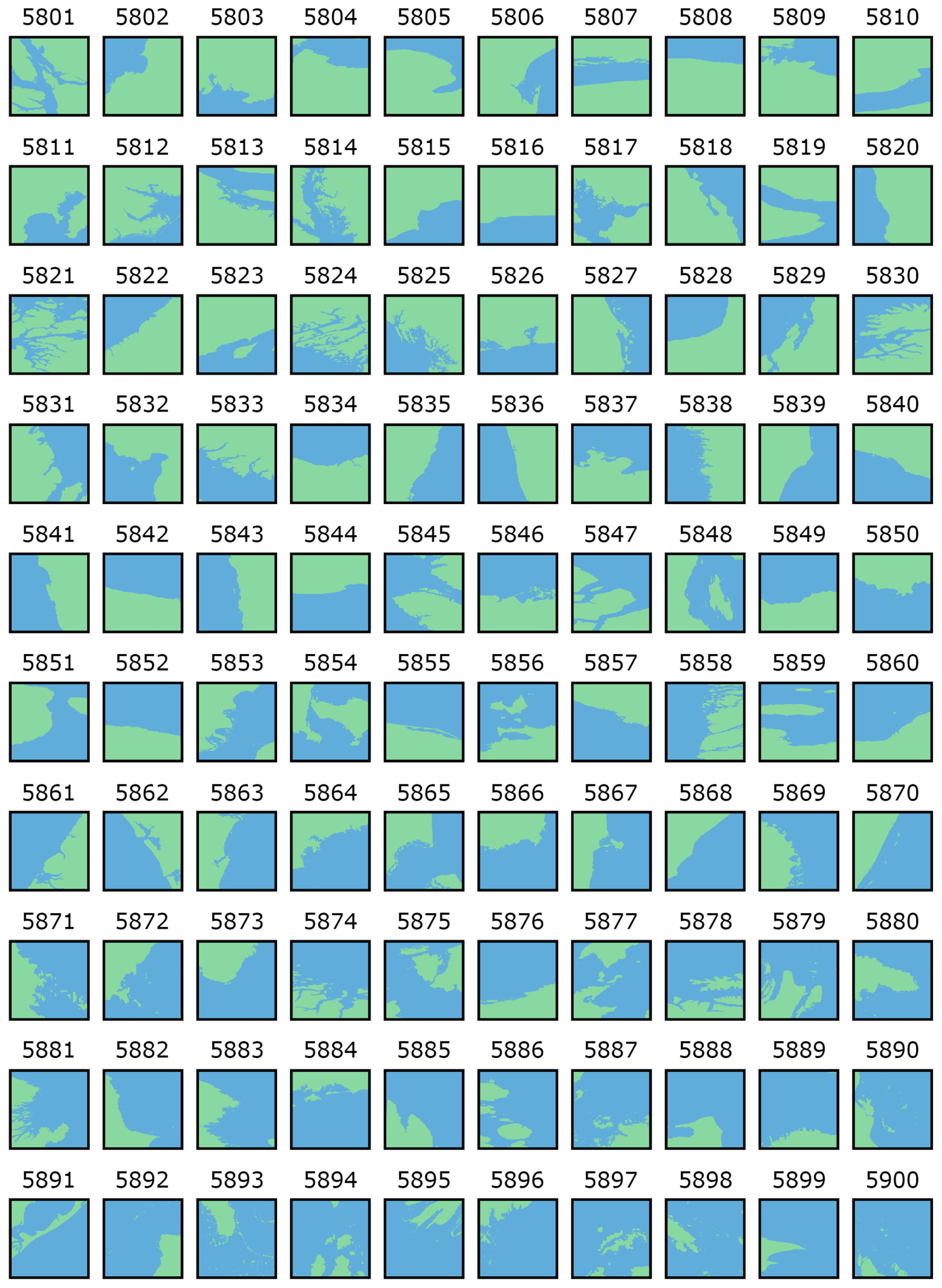
Figure 2 Synthetic thumbnail mosaic displaying all 300 × 300 instances (DEMs) from library A in a bi-colour format.

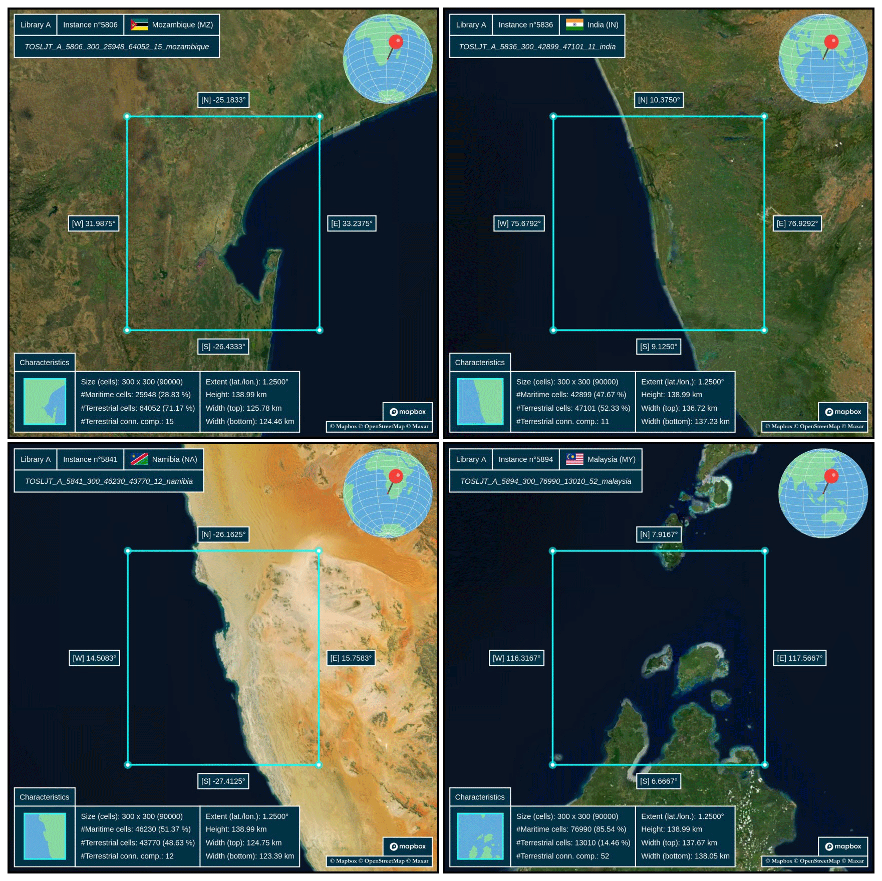
Figure 3 Individual views through annotated satellite imagery of the following 300 × 300 instances from library A: nos. 5806, 5836, 5841, and 5894.

To provide a brief historical context, this catalogue has its origins in work carried out on the optimal configuration of active multistatic sonar networks (MSNs) in order to maximise the insonification (coverage) of a geographical area of interest (AoI). An active MSN is made up of a set of sonar systems in a monostatic and/or bistatic configuration, where each sonar system is a pair consisting of a transmitter (source) and a receiver. Monostatism refers to the case where the two sensors are collocated, and bistatism refers to the case where they are de-located (Cox, 1989; Urick, 1983) (potentially operating several kilometres apart and on two disjointed immersion planes). These sonars can be of several different types: sonobuoys parachuted from an airborne carrier (e.g. maritime patrol aircraft (MPA), helicopter, or drone), dipping sonar from a helicopter, towed array or hull-mounted sonar on a frigate, etc. (Avcioglu et al., 2022). For further information on the subject of optimal configuration of MSN networks, readers are invited to consult Craparo and Karatas (2018), Craparo et al. (2019), Craparo and Karatas (2020), Fügenschuh et al. (2020), Thuillier et al. (2024a), Thuillier et al. (2024d), and Thuillier et al. (2024b). In this context, it was therefore useful to have a variety of AoIs in order to carry out numerical experiments on the optimisation methods developed to configure such networks. As a result, we decided to generate a large number of instances distributed around the world over coastal areas and accompanied by elevation data (bathymetric and topographic) as this is an important aspect of sonar performance. Indeed, until now, there has been no benchmark available for this, and we think it might be beneficial to have a reference with which to compare in the literature. Furthermore, we believe that these instances could find a use outside the framework in which they were devised, i.e. with applications not necessarily related to the configuration of sonar networks.

This article is structured as follows. First, in Sect. 2, we provide essential background information about GEBCO through original visualisations specially derived for the occasion as this constitutes the centrepiece of this catalogue. Then, in Sect. 3, we formally define the instances, including their intrinsic features, the file format, and the naming convention adopted. Subsequently, in Sect. 4, we provide in-depth coverage of the generation procedure designed to populate the present catalogue so as to ensure reproducibility. Finally, we conclude and pinpoint a number of identified prospects for further work in Sect. 6.

2 Background information

GEBCO is a project that was instigated at the beginning of the 20th century by Prince Albert I of Monaco during a commission meeting when the need for a standardised international nomenclature and terminology for bathymetric contour charts was expressed. In addition to working on nomenclature, this same commission, appointed at the 7th International Geographic Congress in Berlin in 1899, was responsible for publishing a general bathymetric chart in paper format, the first edition of which was printed in Paris in 1905 and was called the “carte générale bathymétrique des océans”, which literally translates to General Bathymetric Chart of the Oceans or GEBCO. The aim was straightforward: to provide state-of-the-art information on the shape and depth of the world's seabed. As a result, between 1904 and 1982, there were a total of five paper editions:

• first edition in 1903

• second edition from 1910 to 1930

• third edition from 1932 to 1966

• fourth edition from 1958 to 1973

• fifth and final edition from 1973 to 1982.

Nonetheless, for the third and fourth editions, there was a major reorganisation. Indeed, following the death of Prince Albert I and the dismantling of his scientific team, the project was transferred to the International Hydrographic Bureau (IHB), henceforth known as the International Hydrographic Organisation (IHO). Nowadays, GEBCO operates under the joint auspices of the IHO and the Intergovernmental Oceanographic Commission (IOC) of UNESCO, the latter having been invited to take part in the fifth edition.

The first digital version of GEBCO, named GEBCO Digital Atlas (GDA), on CD-ROM was published in 1994 on the grounds of the fifth edition, with a second updated version in 1997⁴. Building on the success of the GDA, a version called GEBCO One Minute Grid was published in 2003, largely based on the data in the GDA and thus marking the real beginning of the online version of GEBCO. In 2009, an updated version (GEBCO_08 Grid) was put online with a resolution of 30 arcsec. The data points in the latter grid were calculated by combining depths obtained by seabed echography and interpolation between measured points. This interpolation between measured points was guided by satellite-derived gravity data. Updated versions of this grid were put online in 2010 and 2014. Then, a milestone was reached in 2016 when Mr. Sasakawa, chairperson of The Nippon Foundation⁵, decided to partner with GEBCO to work cooperatively to map 100 % of the world's seafloor topography by 2030. The project is called Seabed 2030, and its stated ambition is to produce the definitive, most authoritative and publicly accessible high-resolution bathymetric map of the entire world ocean. Indeed, as of 2023, it is estimated that only 20 % of the oceans have been accurately mapped, the rest being based on interpolation of varying degrees of coarseness. More specifically, the latest GEBCO products are produced by the five centres that make up Seabed 2030, including one global centre and four regional centres, outlined below (the distribution of these centres is detailed hereafter):

• Southern Ocean, Alfred Wegener Institute (AWI), Germany;

• South and West Pacific Ocean, National Institute of Water and Atmospheric Research (NIWA), New Zealand;

• Atlantic and Indian oceans, Lamont Doherty Earth Observatory (LDEO), Columbia University, USA;

• Arctic and North Pacific oceans, Stockholm University (SU), Sweden, and the Center for Coastal and Ocean Mapping at the University of New Hampshire (UNH), USA;

• Global Data Center, British Oceanographic Data Centre (BODC), National Oceanography Centre (NOC), UK.

The overall organisation is as follows. The four regional centres compile the various bathymetric data (largely based on multibeam echo sounder data) for their respective areas of interest and supply them in grid form to the global centre, which is responsible for delivering the global grid by splicing the pieces together. Thus, since the Seabed 2030 initiative, there have been the 2019, 2020, 2021, 2022, and 2023 versions, with a resolution of 15 arcsec for all these grids. From 2019 onwards, the grids have had the following features:

• a horizontal extent from $\mathrm{179}\mathit{°}{\mathrm{59}}^{\prime }{\mathrm{52.5}}^{\prime \prime }$ W (−179.9979167°) to $\mathrm{179}\mathit{°}{\mathrm{59}}^{\prime }{\mathrm{52.5}}^{\prime \prime }$ E (179.9979167°)

• a vertical extent from $\mathrm{89}\mathit{°}{\mathrm{59}}^{\prime }{\mathrm{52.5}}^{\prime \prime }$ S (−89.9979167°) to $\mathrm{89}\mathit{°}{\mathrm{59}}^{\prime }{\mathrm{52.5}}^{\prime \prime }$ N (89.9979167°)

• 43 200 (rows) × 86 400 (columns) = 3 732 480 000 unique pixels (i.e. cells).

All the pixels in the GEBCO grid are referenced according to the horizontal coordinate reference system (CRS) WGS84 (EPSG:4326) and according to the vertical CRS mean sea level (MSL) height (EPSG:5714). For more information on CRS, please refer to Sect. A. There is also a reference for the combination of these two CRS (compound CRS), which can be found under the code EPSG:9705 (WGS 84 + MSL height), as discussed in Appendix A. Besides, as a reminder, the elevation data are “pixel-centre” registered in the GEBCO grid, meaning that it is the elevation at the centre of a cell with a resolution of 15 arcsec (approximately 460 m × 460 m at equatorial level). This resolution of 15 arcsec makes the plate carrée projection the most intuitive for visualisation (see Appendix A for more details on projections) and will therefore be used throughout this article. Indeed, the meridians are projected onto regularly spaced vertical lines, and the parallels are projected onto regularly spaced horizontal lines, giving us a subdivision of space into cells (pixels) of equal size, i.e. a grid. This projection thus facilitates the conversion between geographical coordinates and pixels, which makes it a standard for a large number of global raster datasets including GEBCO. The projected coordinate system (PCS) associated with this projection has the code EPSG:54001 and depends on the geographic (geodetic) coordinate system (GCS) WGS84.

Finally, note that the latest grids are based on version 2.5.5 of the SRTM15+ (Shuttle Radar Topography Mission with 15 arc resolution) dataset⁶ (Becker et al., 2009; Olson et al., 2014; Tozer et al., 2019), augmented with bathymetric data from the Seabed 2030 regional centres. The SRTM dataset is a fusion of terrestrial topography and an estimate of seabed topography using altimetry (depth predicted from gravity). Version 2.5.5 is similar to version 2.1 (Tozer et al., 2019) but includes predicted depths based on the V32 (Sandwell et al., 2021) gravity model.

Figure 4 shows the difference between the areas that have been mapped accurately and the global GEBCO grid as of 2023, with interpolation on the unmapped areas (around 80 %). Figure 5 focuses on two given zones in order to show the heterogeneity of the input data from which the global GEBCO grid is produced. Finally, Fig. 6 shows a three-dimensional view of the GEBCO 2023 grid in various representations, including a detailed close-up of two areas of interest.

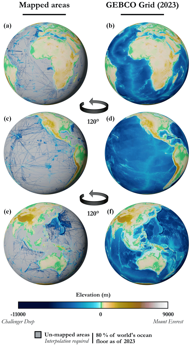
Figure 4 Areas mapped accurately through measured depth values on the left and complete GEBCO 2023 grid on the right for comparative purposes (flat geometry, textures colour-coded for elevation, no shaded relief).

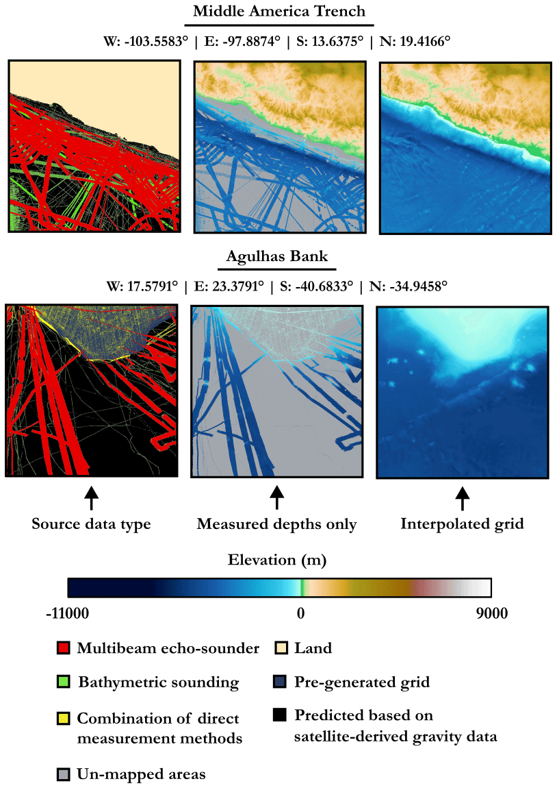
Figure 5 Focus on two areas of interest (AoIs) with details of the source data types (not exhaustive list) in order to demonstrate the inherent heterogeneity of the GEBCO global elevation model.

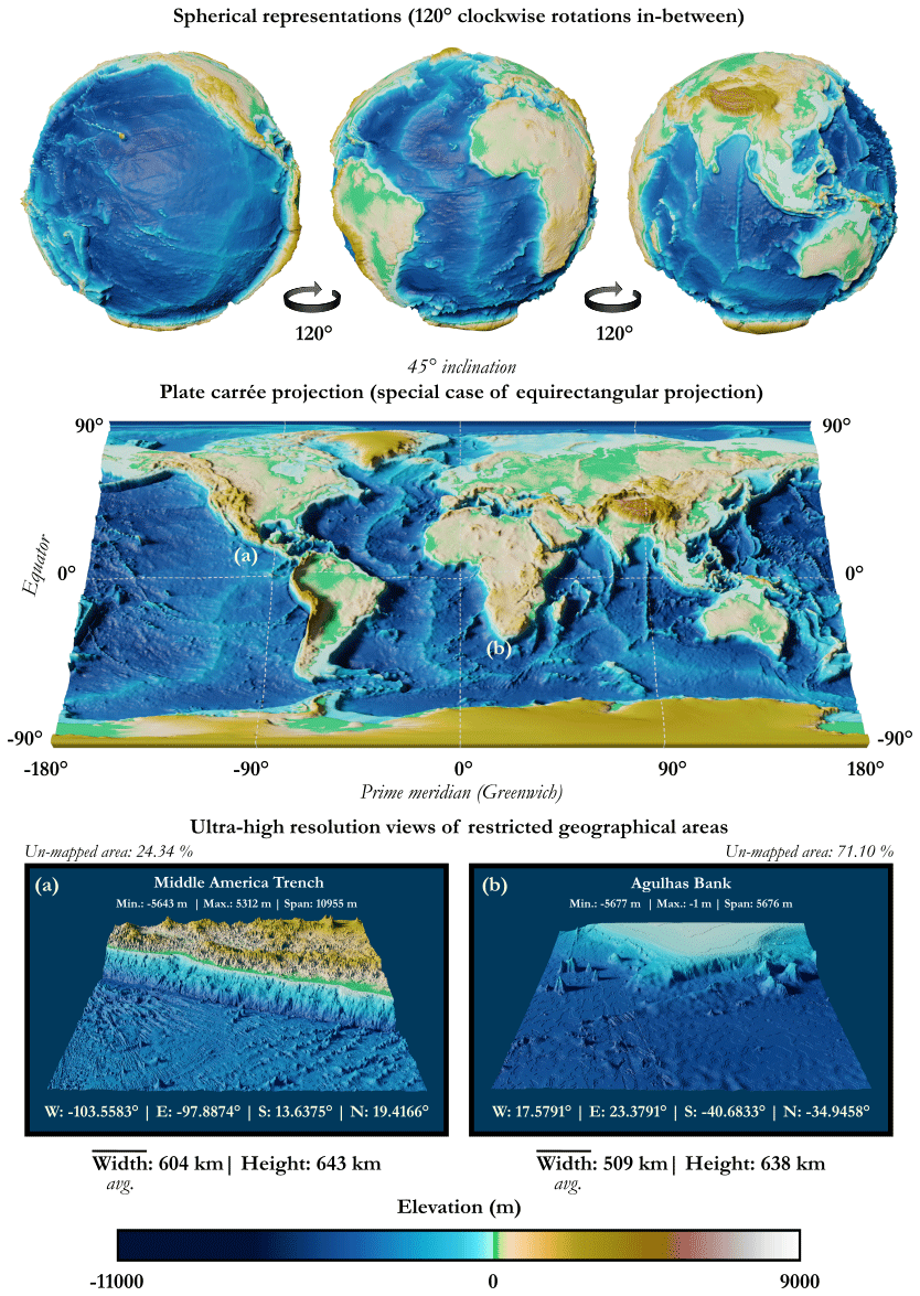
Figure 6 Visualisation of the global digital elevation model (DEM) made available by GEBCO as of 2023 using spherical representations, a planar projection (90° graticule), and ultra-high-resolution views of restricted geographical areas (textures colour-coded for elevation and relief exaggeration on the vertical axis for illustrative purposes).

3 Instances

In this third section, we are going to take a closer look at the formal description of the instances, including their intrinsic features, file formats, naming conventions, overall catalogue organisation, and some visualisation guidelines.

3.1 Intrinsic features

The instances in the catalogue have a number of common intrinsic features, which we will highlight in the following. First of all, the different instances have a unique maritime-connected component and have a ratio of maritime cells ranging from 25 % to 95 % so as to cover a whole spectrum of different coastline geometric configurations. It should be noted that the decision to have only a single maritime-connected component stems from the application for which these instances were originally intended: the configuration of MSNs. Furthermore, there are terrestrial cells that are actually inland waters which have been artificially filled in because, for the intended application, there was no reason to consider them. Nevertheless, we were keen not to lose the information corresponding to inland waters that had been artificially filled in, and so we opted for a compromise that would allow us to retain the elevation data associated with them⁷. For example, if an isolated maritime cell had an elevation of −13 m then we would replace this elevation with 999913, which would then be decoded as a character string, with the number 9999 encoding the fact that this is inland water (this works because there are no summits above this altitude on Earth). In particular, it is useful to have access to the elevation data of isolated maritime cells if one wishes to carry out re-sampling (up or down).

3.2 File format

The various instances (DEMs) are delivered in the text-based Esri ASCII grid format (.asc), which is proving to be a suitable medium for distributing such DEMs for the following reasons:

• it is human-readable;

• it is not dependent on any particular hardware (plain text), which makes it easier to transfer across platforms (highly portable);

• it can be used (export and/or import) in most GIS software⁸, such as QGIS, gvSIG, or SAGA GIS, to name just a few of the open alternatives;

• it is compatible with any horizontal CRS, GCS, or PCS, and a vertical CRS as long as this is specified elsewhere;

• it is easy to parse through a script if required;

• it is reasonably compact when files are compressed.

An alternative to this type of text-based format is to use binary formats such as GeoTIFF⁹ (Tag Image File Format: .tiff) or NetCDF¹⁰ (Network Common Data Form: .nc) as proposed natively by GEBCO. The main advantages of using such formats are an increased speed of read/write (I/O) operations as there is no need for two-way conversion¹¹, and a reduced storage footprint¹². Indeed, for the global coverage provided by GEBCO in 2022, it takes around 8 GB for the binary format compared to 20 GB for the text format without compression (however, the gap narrows to 4 and 5 GB, respectively, after compression). Another advantage of the NetCDF and GeoTIFF formats is the possibility of having multiple bands or strips (i.e. dimensions), whereas this is impossible with the Esri ASCII format: one file per band is required. However, the added efficiency of binary files comes with the major drawback that it is not directly readable and therefore not very user-friendly when it comes to obtaining an overview of the data, plus it can be difficult to fix corrupted files. In the end, since performance is not paramount, storage is a lesser problem, and we only need a single band for the instances under consideration (i.e. elevation), we have therefore opted for this text-based format for the above-mentioned advantages.

A file in the Esri ASCII grid format consists of two consecutive parts:

• a header containing a certain amount of metadata about the grid, such as the geographical extent¹³ and the grid resolution (i.e. the cell size)

• the data part, where an integer or floating-point numerical value is associated with each cell of regular angular extent (see cell size field), which, here, corresponds to the elevation taken at the centre point of the latter (see the Introduction for further details).

More formally, this takes the following form: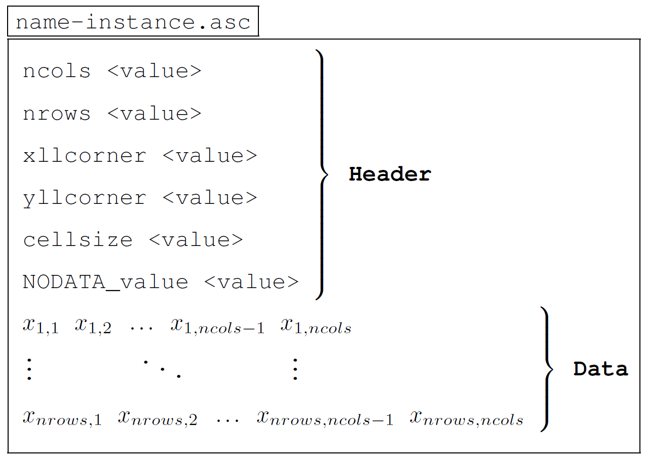
where

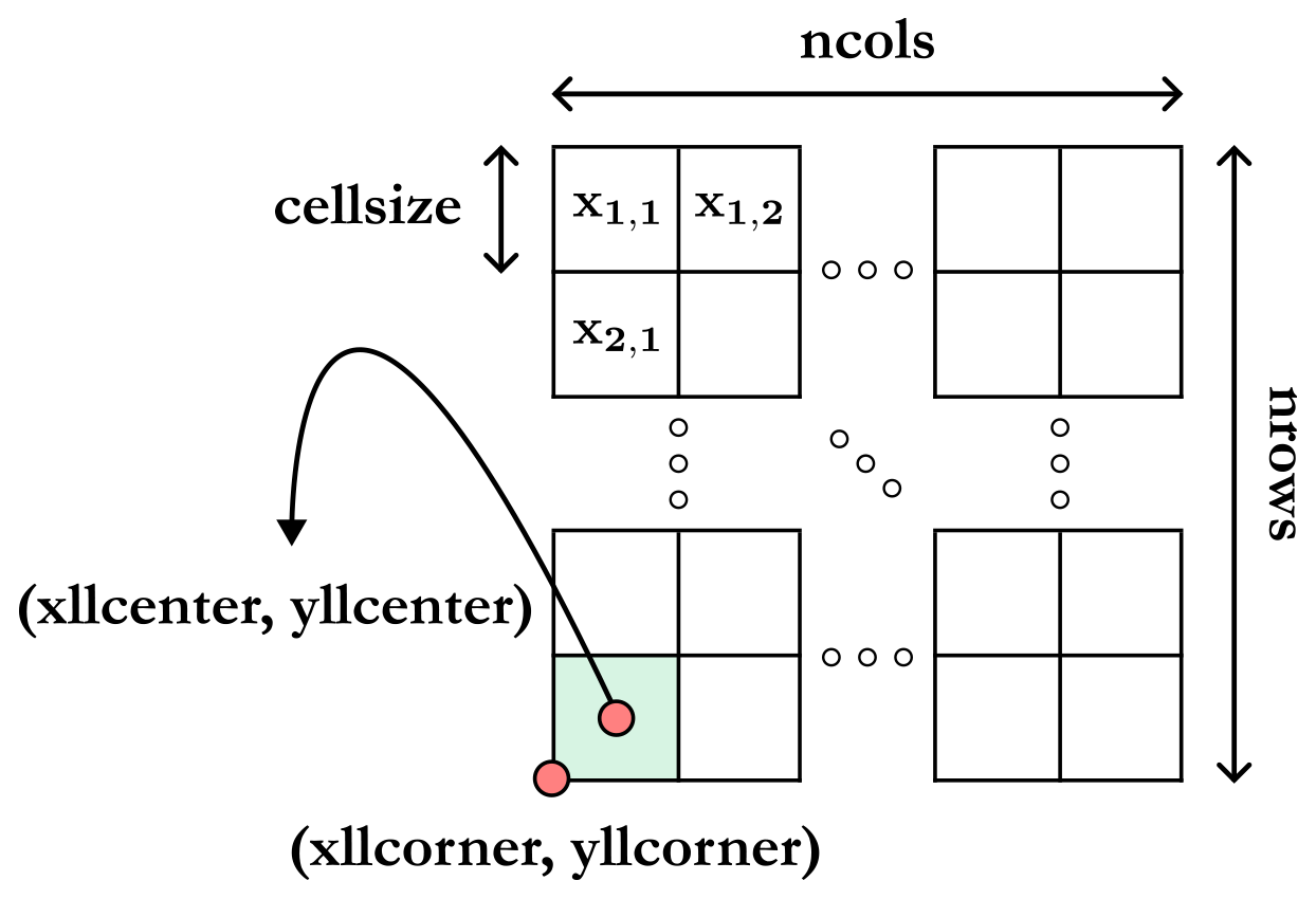
• ncols (integer) and nrows (integer) correspond, respectively, to the number of columns and rows in the grid;

• xllcorner (float) and yllcorner (float) are, respectively, the x coordinate (i.e. longitude) and the y coordinate (i.e. latitude) of the grid origin located at the lower-left corner of the lower-left cell, expressed in the horizontal CRS WGS84 (EPSG:4326 (https://epsg.io/4326, last access: 2 October 2024)) with the decimal degrees (DD) notation;

• cellsize (float) is the length of one side of a square cell (i.e. both height and width) in the same reference unit as the origin (DD), corresponding to approximately 0.00417° in the case of the GEBCO grid (i.e. 15 arcsec);

• NODATA_value (float or integer) is the default value assigned when an input is missing or unknown;

• xi,j (float or integer) is the elevation value assigned to the cell (i,j) at the intersection of row $i\in \left[\right[\mathrm{1},\mathrm{nrows}\left]\right]$ and column $j\in \left[\right[\mathrm{1},\mathrm{ncols}\left]\right]$, given in the vertical CRS MSL height (EPSG:5714 (https://epsg.io/5714, last access: 2 October 2024)), i.e. in metres referenced to mean sea level (positive upwards).

Note that, in our case, we will only have integer values for elevations (x_i,j) and the NODATA_value, as is the case for the data retrieved from the GEBCO global grid. A visual representation of the different elements defining a grid in Esri ASCII format is available in Fig. 7. In addition, a number of general remarks about this particular format are listed hereafter if anyone would like to modify or propose new instances:

• The values assigned to the various cells are given in row-major order (i.e. left to right and top to bottom) and must be separated by a single-space character. Moreover, in theory, no carriage return is required at the end of each row of the grid because the number of columns is known, but, in practice, this makes it more legible. In either case, the number of values must be equal to the number of rows (nrows) times the number of columns (ncols), i.e. one single value per cell.

• It is possible to define the origin of the grid alternatively by using the keywords xllcenter (float) and yllcenter (float), which then locates the grid in the centre of the lower-left cell.

• The NODATA_value keyword is optional but strongly recommended.

• The various keywords in the header are not case-sensitive, although it is recommended that they be consistent for ease of use.

Figure 7 Schematic view of the structure of an Esri ASCII grid.

For illustrative purposes, a didactic example of a 20×20 grid showing the structure of all the catalogue instances in this particular format is shown hereafter.

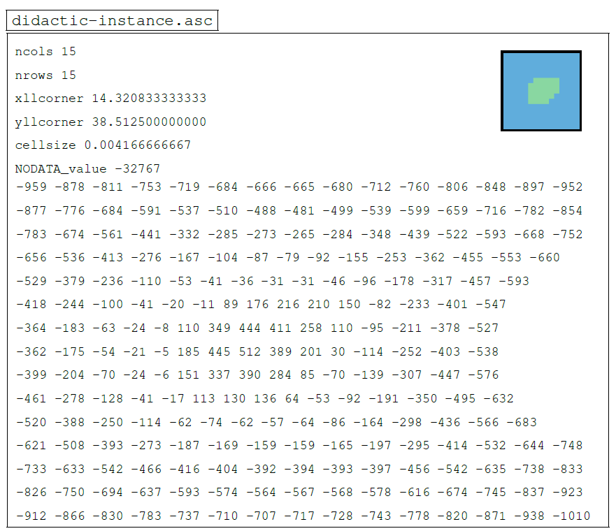
More specifically, this is the volcanic island of Alicudi, part of the Aeolian archipelago in the Tyrrhenian Sea and lying to the north of Sicily in Italy. Although a bi-colour thumbnail gives a rough idea of the geographical configuration of the instance under consideration, Fig. 8 presents a much more detailed visualisation through the compilation of numerous data from various sources. This figure is structured as follows.

Firstly, the texture in the upper plane corresponds to a satellite view taken from a compilation of data from the Sentinel-2 mission of the Copernicus programme operated by the ESA (European Space Agency) in the three bands of the visible spectrum (B2, B3, and B4) over a sliding year in order to obtain an image with as few clouds as possible. This texture was then post-processed using artificial intelligence in order to remove certain artefacts such as boat tracks or dwellings, the idea being to obtain the purest texture possible, representative of the island's topography and free from anthropogenic activity. A DEM is then added to this base texture, using topographic data from NASA's SRTMGL1 (Shuttle Radar Topography Mission (SRTM) Global 1 arcsec (GL1)) version 3 dataset, with a resolution of around 30 m × 30 m. Note that the horizontal CRS is WGS84 (EPSG:4326), like the GEBCO grid, but the vertical CRS here is the EGM96 (Earth Gravitational Model from 1996) height (EPSG:5773), and so there may be a difference of several metres with the GEBCO elevations, which are referenced to the vertical CRS MSL height (EPSG:5714). At equivalent resolution, however, this error would be negligible as these are two gravity-related models linked to the geoid, but, here, the GEBCO data (15 arcsec) have a much lower resolution than the SRTMGL1 data (1 arcsec), and this can lead to large differences (negligible, nevertheless, for our use). In addition, these elevation data were interpolated afterwards to obtain a rendering as close as possible to reality, avoiding the asperities associated with the data resolution. It should also be noted that the proportions have not been preserved and that the z axis (vertical) has been distorted in order to achieve a better rendering (the same applies to the bottommost plane). Also, for the three parts of the figure, these representations are based on an equirectangular (or equidistant cylindrical) projection of the globe, i.e. forming a Cartesian grid made up of identical squares (pixels), a projection which is used for global raster datasets such as GEBCO or SRTMGL1 because it facilitates conversions between geographical coordinates and pixels (as discussed earlier in Sect. 2).

In the middle section, we have the grid with the bathymetric and topographic data supplied by GEBCO. As a reminder, the GEBCO grid is pixel-centre registered, and so the elevations (in metres) correspond to the points at the centre of each of the cells (pixels) with a resolution of 15 arcsec, i.e. approximately 460 m × 460 m at equatorial level. A vertical column showing the elevations in plain text at GEBCO resolution is also provided to show the transition between the top and middle planes for an area of 3 × 3 pixels.

On the lower plane, we have this same grid, but this time with a three-dimensional representation, with the elevation represented on the z axis (proportions not respected, same distortion as for the upper plane). As discussed above, the resolution is lower than with the data from SRTMGL1, and this can now be seen (interpolation aside), but, this time, we have the bathymetric data as well, which is the key feature of the GEBCO grid.

In addition, a picture of the island with an east–west approach (i.e. a heading of 270°) is also available at the bottom left of the figure. Finally, a map on the bottom right-hand side gives a rough location for the island of Alicudi, whose GPS coordinates in DMS format are also shown on the right-hand side of the base in the horizontal CRS WGS84 (EPSG:4326). This map was produced using Blue Marble: Next Generation images, in this case the December texture with topography and bathymetry, made available by NASA Visible Earth.

Figure 8 Detailed visualisation of the didactic instance.

3.3 Naming convention

This section describes the naming convention used to designate all the different instances of the catalogue spread across the three libraries A, B, and C. First of all, an instance is formally referred to under the following full format:

TOSLJT_library_id_n_m_t_nb-tcc_country.

In the above, we have the following:

• TOSLJT refers to the initials of the authors (Thuillier, Olteanu, Sevaux, Le Josse, and Tanguy).

• Second, library (string) corresponds to the parent library.

• Third, id (string) is the unique identifier of an instance within the parent library. This unique identifier is coded on a string of four characters (examples: 0001, 0015, 0108, and 1204 for instances no. 1, no. 15, no. 108, and no. 1204, respectively). Furthermore, for a given dimension, the 100 instances are ranked in ascending order in terms of the number of maritime cells so that the instance with the smallest identifier corresponds to the instance with the fewest maritime cells. That said, it is possible for a lower-dimensional instance to have more maritime cells.

• Following this, n (integer) corresponds to the dimensions of the instance (example: n=10 means that we are dealing with an instance with dimensions of 10 × 10). Note that we only need one integer as we are dealing exclusively with square grids.

• Following this, m (integer) and t (integer) correspond to, respectively, the number of maritime cells and the number of terrestrial cells.

• Following this, nb-tcc (integer) refers to the number of terrestrial connected components.

• Finally, country (string) is the country of affiliation.

For example, the instance with the name

TOSLJT_A_0108_15_69_156_1_australia

reveals that it is instance no. 108 from library A, which is a 15×15 grid with 69 maritime cells, 156 terrestrial cells, and 1 terrestrial connected component and is located on a coastline of Australia.

Finally, a particular instance of the catalogue can be uniquely and unambiguously identified by simply using the following short format:

TOSLJT_library_id,

which can be useful for referring to a set of instances during numerical experiments. For the above example, this would therefore be TOSLJT_A_0108.

4 Generation procedure

In this fourth section, we will take an in-depth look at the procedure for generating the various instances, which will be subdivided into key sub-steps.

4.1 Seed selection

The first step consists of randomly drawing a geographical point (a seed) from one of the world's coastlines, i.e. on a natural physical boundary on the edge of an ocean or sea, either on a continental land-mass or on an ocean island. Indeed, we filter out lakes, rivers, islands on lakes, and ponds on islands within lakes because these cases actually exist and were artefacts: there are no (or only partial) bathymetric data available for these places¹⁴ in the global grid provided by GEBCO. To achieve this, we have retrieved a dataset listing all the coastlines across the globe in the form of polylines made up of a set of points with geographical coordinates in the horizontal CRS WGS84 (EPSG:4326) and have arranged them in such a way as to retain only the coastlines of interest to us (see Figs. 9 and 10 for an illustration of the different levels of coastline mentioned; case no. 1 is the one adopted here). This dataset is the Global Self-consistent, Hierarchical, High-resolution Geography Database (GSHHG) made available by Wessel and Smith (1996), which is based on three public-domain datasets: World Vector Shorelines (WVS)¹⁵ (Soluri and Woodson, 1990), CIA World Data Bank II (WDBII)¹⁶ (Gorny, 1977), and Atlas of the Cryosphere (AC)¹⁷ (Scambos et al., 2007). It should also be noted that we have excluded the Antarctic from this catalogue as it is treated differently in the GEBCO dataset: there are parts corresponding to the elevations both above and below ice. The difference between grounding-line and ice-front boundaries for the coastlines shown in Fig. 10 is illustrated in Fig. 11.

Figure 9 Illustration of the different levels of coastlines using a plate carrée projection (special case of an equirectangular projection centred on the Equator), part 1/2.

Figure 10 Illustration of the different levels of coastlines using a plate carrée projection (special case of an equirectangular projection centred on the Equator), part 2/2.

Figure 11 Illustration of the difference between ice-front boundary and grounding-line boundary for the Antarctic.

We take this opportunity to mention a pitfall we encountered when producing this catalogue: the spatial distribution of instances was originally extremely unbalanced. The reason is illustrated in Fig. 12 and is as follows. The resolution of the coastlines was far too excessive, and there are places in the world made up of tens of thousands of small islands (e.g. the Archipelago Sea¹⁸, with an estimated 50 000 islets, and the Canadian Arctic Archipelago, with nearly 40 000 islets), which led to a genuine imbalance in the spatial distribution of instances. Indeed, there was a greater probability of drawing a seed from one of these regions. One of the solutions envisaged to overcome this problem was (step 1) to filter out islands below a certain size and (step 2) to weight the probability of drawing a seed from a land-mass or an island according to its size and, therefore, depending on the number of segments (by extension, points) used for discretisation. This solution has been preferred, providing a fairer spatial distribution of instances throughout the globe. Another solution to this issue lies in the use of a geometric data compression algorithm such as the Douglas–Peucker algorithm (Douglas and Peucker, 1973), sometimes called the Ramer–Douglas–Peucker algorithm, which simplifies a polygon or a broken line (polyline) by removing some of the points. This would have had the effect of eliminating the smallest islands and thus reducing the number of points from which to choose a seed (particularly by eliminating geographically neighbouring points). However, such an algorithm tends to deteriorate the quality of the coastline contouring, as illustrated in Fig. 13, and this solution was not chosen for this reason.

Figure 12 Illustration of the pitfall encountered and the filtration procedure put in place for undersized emerged lands (focus is on part of the Baltic Sea subject to numerous islets).

Figure 13 Illustration of the Douglas–Peucker geometric data compression algorithm for coastline simplification at three levels of resolution.

From now on, we have a seed with coordinates $s=({\mathrm{lat}}_s,{\mathrm{long}}_s)\in [-\mathrm{90},\mathrm{90}]\times [-\mathrm{180},\mathrm{180}]$ representing the centre of the current grid of dimension n∈ℕ (square here) and whose bounding box is defined by the bounds

• north = lat${}_s+(\frac{n}{\mathrm{2}}\cdot \text{cell size})$,

• south = lat${}_s-(\frac{n}{\mathrm{2}}\cdot \text{cell size})$,

• west = long${}_s-(\frac{n}{\mathrm{2}}\cdot \text{cell size})$,

• east = long${}_s+(\frac{n}{\mathrm{2}}\cdot \text{cell size}$).

As a reminder, cell size corresponds to the size of a cell, i.e. 15 arcsec for the GEBCO global grid or approximately 0.00417°. Figure 14 shows a current grid determined by the drawing of a seed, with the GEBCO grid graticule in the background (in grey). Note that, at this stage, the two do not necessarily coincide, and the probability of this happening is actually very low.

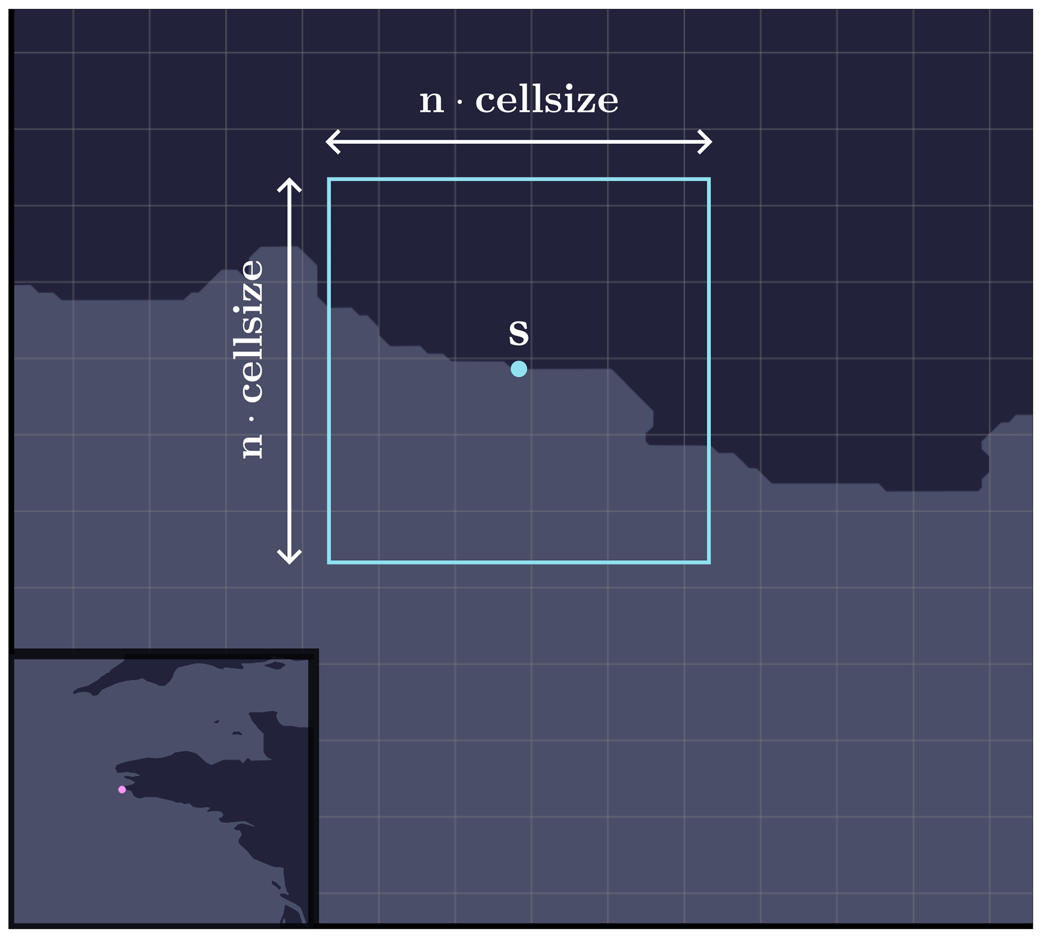
Figure 14 Illustration of a current grid of dimension n determined by the drawing of a seed on a coastline (GEBCO graticule in grey, i.e. 15 arcsec).

4.2 Offset

Once we have a seed located on a coastline (continental land-mass or ocean island), we are going to offset it in such a way as to introduce more or fewer maritime cells and a little more variability¹⁹. To do this, we are going to offset the seed by randomly drawing

• a vertical displacement ${\mathit{\lambda }}^{\updownarrow }\in [-\frac{n}{\mathit{\delta }}\cdot \text{cell size},\frac{n}{\mathit{\delta }}\cdot \text{cell size}]$,

• a horizontal displacement ${\mathit{\lambda }}^{\leftrightarrow }\in [-\frac{n}{\mathit{\delta }}\cdot \text{cell size},\frac{n}{\mathit{\delta }}\cdot \text{cell size}]$,

where δ∈ℝ is a parameter. For this catalogue, we choose δ=3 so that there is a minimum overlap between the old and new zones. The seed is therefore moved to the point

$$\begin{array}{}\text{(1)}& s^{\prime }=\left({\mathrm{lat}}_s+{\mathit{\lambda }}^{\updownarrow },{\mathrm{long}}_s+{\mathit{\lambda }}^{\leftrightarrow }\right).\end{array}$$

The principle of offset is illustrated in Fig. 15. In addition, it was also possible to envisage a displacement in a circular region around the seed and not in a square region, as has been done here. The difference between these two possibilities is illustrated in Fig. 16.

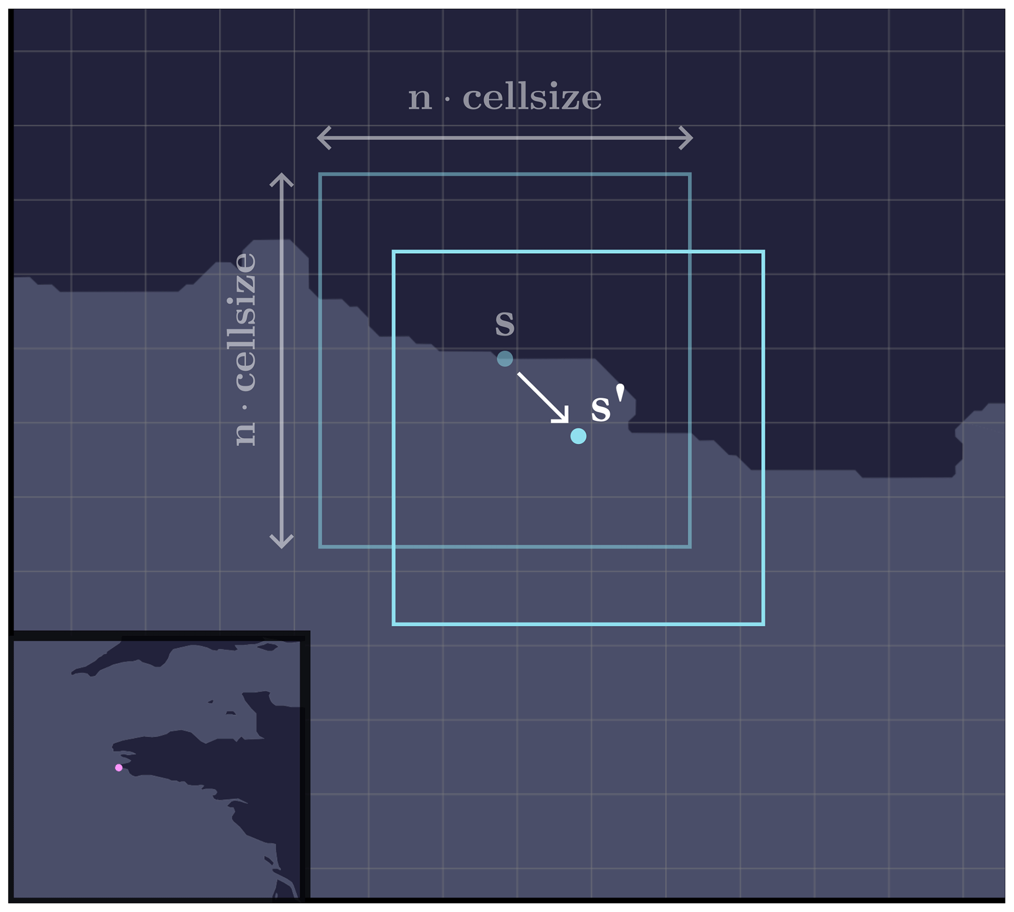
Figure 15 Illustration of the seed offset mechanism (GEBCO graticule in grey, i.e. 15 arcsec).

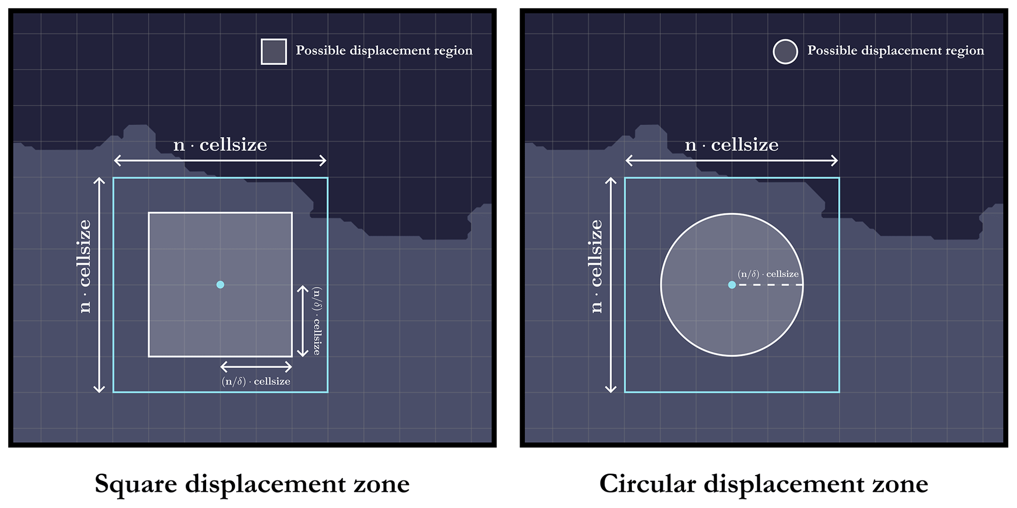
Figure 16 Two possibilities for the offset: circular or square displacement (GEBCO graticule in grey, i.e. 15 arcsec).

4.3 Recalibration on the GEBCO grid

Now that we have offset the seed, all that remains is to align the current grid with the GEBCO grid graticule (if this is not the case; otherwise, we move on to the next step). To do this, we need to distinguish between two cases depending on whether n is even or odd.

4.3.1 Odd case

In the odd case illustrated in Fig. 17, the seed is moved to the centre of the cell in which it is located, i.e. at the coordinates

$$\begin{array}{}\text{(2)}& \begin{array}{rl}s\mathrm{"}& =\left(⌊{\displaystyle \frac{{\mathrm{lat}}_{s^{\prime }}}{\text{cell size}}}⌋\text{cell size}+{\displaystyle \frac{\text{cell size}}{\mathrm{2}}},\right.\\ & \left.⌊{\displaystyle \frac{{\mathrm{long}}_{s^{\prime }}}{\text{cell size}}}⌋\text{cell size}+{\displaystyle \frac{\text{cell size}}{\mathrm{2}}}\right).\end{array}\end{array}$$

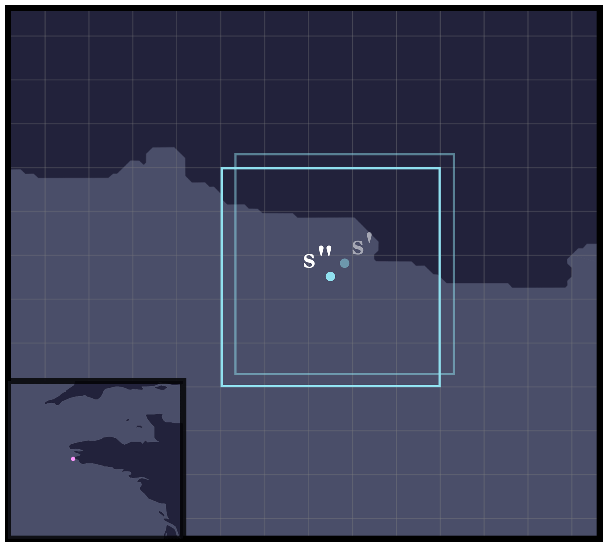
Figure 17 Illustration of the procedure for recalibrating the current grid on the GEBCO graticule: odd case (GEBCO graticule in grey, i.e. 15 arcsec).

4.3.2 Even case

In the even case illustrated in Fig. 18, there is a choice to be made: the seed (i.e. the centre of the current grid) can be moved to one of the four corners of the cell in which it is located: southwest, northwest, northeast, or southeast. Here, we have chosen to shift the seed to the corner that minimises the displacement distance (i.e. to the corner closest to the seed after offset). The seed is therefore moved to the point

$$\begin{array}{}\text{(3)}& s\mathrm{"}=\arg \underset{x\in X}{min}\left(d\right(s^{\prime },x\left)\right),\end{array}$$

where $X=\mathit{\{}\text{southwest},\text{northwest},\text{northeast},\text{southeast}\mathit{\}}$, and d is the great-circle (orthodromic) distance between two geographical points and

• $\text{southwest}=\left(⌊\frac{{\text{lat}}_{s^{\prime }}}{\text{cell size}}⌋\text{cell size},⌊\frac{{\text{long}}_{s^{\prime }}}{\text{cell size}}⌋\text{cell size}\right)$,

• $\text{northwest}=\left(⌈\frac{{\text{lat}}_{s^{\prime }}}{\text{cell size}}⌉\text{cell size},⌊\frac{{\text{long}}_{s^{\prime }}}{\text{cell size}}⌋\text{cell size}\right)$,

• $\text{northeast}=\left(⌈\frac{{\text{lat}}_{s^{\prime }}}{\text{cell size}}⌉\text{cell size},⌈\frac{{\text{long}}_{s^{\prime }}}{\text{cell size}}⌉\text{cell size}\right)$,

• $\text{southeast}=\left(⌊\frac{{\text{lat}}_{s^{\prime }}}{\text{cell size}}⌋\text{cell size},⌈\frac{{\text{long}}_{s^{\prime }}}{\text{cell size}}⌉\text{cell size}\right)$.

Figure 18 Illustration of the procedure for recalibrating the current grid on the GEBCO graticule: even case (GEBCO graticule in grey, i.e. 15 arcsec).

4.4 Retrieving elevations

At this stage, all we need to do is go through all the cells (pixels) in the current grid and retrieve their elevations using the global GEBCO grid. This involves mapping a pixel (i,j) in the current grid to a pixel $(i^{\prime },j^{\prime })$ in the GEBCO global grid reference data file in Esri ASCII format. The main difficulty arises from the fact that the global GEBCO grid is subdivided into several files or tiles. Hence, for each pixel (i,j) in the current grid, we need to know in which tile (sub-file) it is located and to which pixel $(i^{\prime },j^{\prime })$ it corresponds. Indeed, the same current grid can straddle several tiles at the same time.

Using grid notation for tiles, i.e. with (x,y) being the tile located on row x and column y, a pixel (i,j) is then located on

• tile $(x,y)=\left(⌊\frac{\mathrm{90}-{\text{lat}}_{(i,j)}}{h}⌋+\mathrm{1},⌊\frac{{\text{long}}_{(i,j)}+\mathrm{180}}{w}⌋+\mathrm{1}\right)$,

• pixel $(i^{\prime },j^{\prime })=\left(⌊\frac{\left(\right(\mathrm{90}-(x-\mathrm{1})h\left)\right)-{\text{lat}}_{(i,j)}}{\text{cell size}}⌋\right.$, $\left.⌊\frac{({\text{long}}_{(i,j)}-(-\mathrm{180}+(y-\mathrm{1})w\left)\right)}{\text{cell size}}⌋\right)$,

where h and w correspond to, respectively, the width and height (in decimal degrees) of each of the tiles (regular subdivision), and lat_(i,j) and long_(i,j) correspond to, respectively, the latitude and longitude of the point at the centre of cell (i,j). The principle is summarised in Fig. 19.

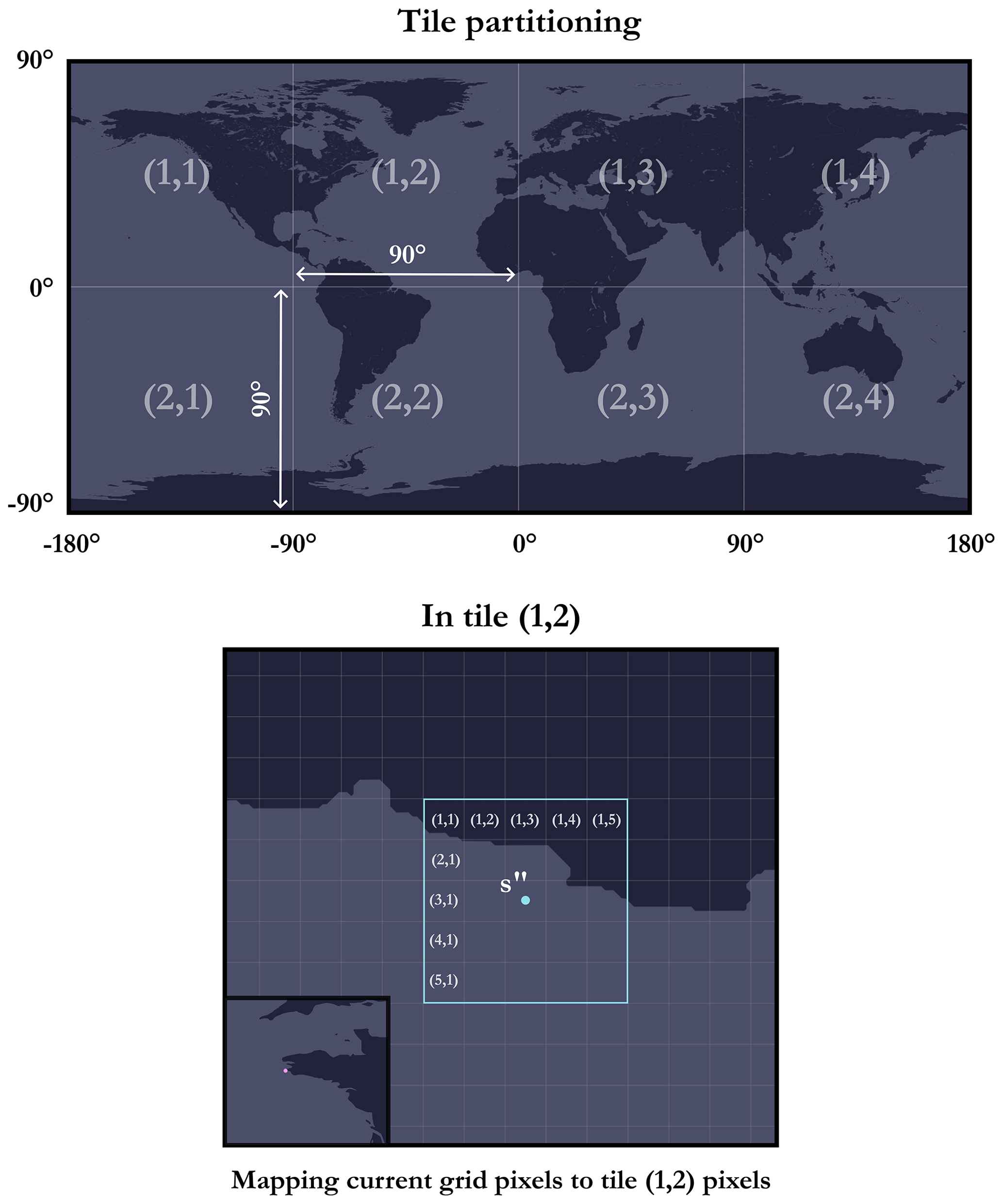
Figure 19 Illustration of the procedure for retrieving elevations of the different cells (pixels) in a current grid using a global grid subdivided into tiles.

4.5 Selection criteria

Now that we have retrieved elevations for the entire grid, we need to ensure that the instance meets certain criteria in order to decide whether or not to accept it. In Sect. 3.1, we stated that an instance must have a unique maritime-connected component and a ratio of maritime cells lying between 25 % and 95 %. However, it is essential to exercise increased accuracy in this regard due to the presence of a subtlety. Indeed, in the case of instances generated from real geographical locations, it is highly unlikely that there will be a unique maritime-connected component, and so we had to resort to a few tricks to overcome this technical challenge. This is particularly the case where there are inland waters such as ponds, lakes, or rivers. Therefore, in practice, the true criteria for selecting an instance are as follows:

• The weight of the main maritime-connected component must be at least 90 % of the weight of the total maritime cells (inland waters included).

• There must be a ratio of maritime cells of between 25 % and 95 % after inland waters, if any, have been artificially filled in (no more than 10 %).

The reason for choosing a minimum of 90 % for the weight of the main connected component is that we did not want to deteriorate the instances excessively by artificially filling in the inland waters; it was therefore necessary to impose an upper bound on their presence (i.e. 10 % in this catalogue).

To achieve this, a given instance (DEM) has been transformed into a graph where each maritime cell represents a vertex and the edges embody the connections between adjacent cells. We have opted for the case where a given maritime cell has four direct neighbours: west, east, south, and north. This is an arbitrary implementation choice, and we could also have considered the alternative of taking into account the diagonal cells (see Fig. 20 for an overview of the differences).

Figure 20 Illustration of the two alternative ways of defining the neighbours of a given cell and the possible implications when this is implemented in a particular instance.

With such a graph, it is now possible to determine the maritime-connected components; see He et al. (2017) for more details. If a given instance is accepted, the set of isolated maritime cells (inland waters) that are not in the main connected component are then artificially filled in as discussed in Sect. 3.1. Finally, Fig. 21 illustrates this with two columns: one for accepted instances (meeting the criteria) and one for rejected instances²⁰.

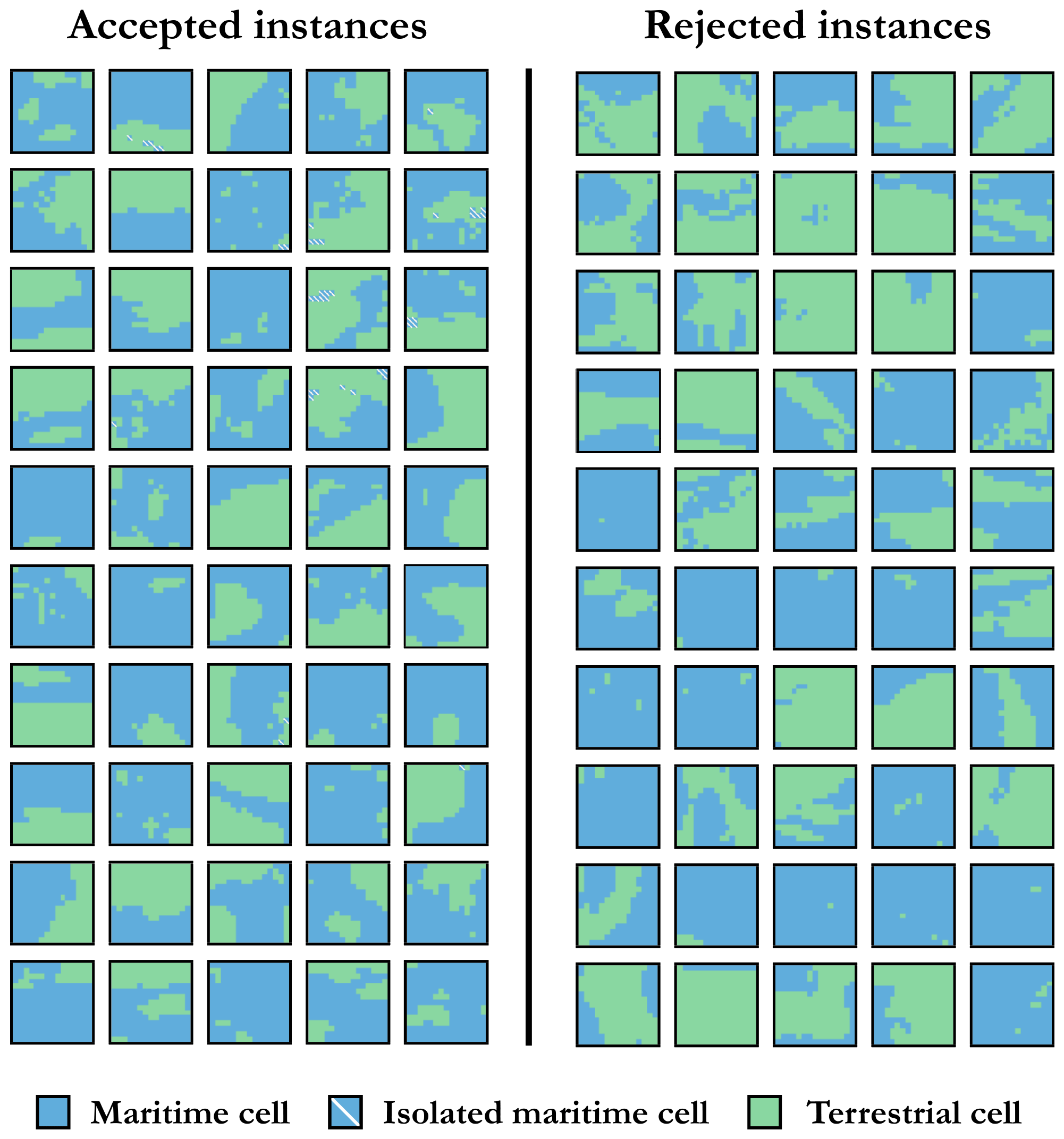
Figure 21 Examples of instances (n=15) that were accepted as meeting the selection criteria and instances that were rejected.

4.6 Reverse geocoding

Once the instance has been approved, we will try to determine the country to which it belongs so that we can proceed with the naming process, in accordance with the convention discussed in more detail in Sect. 3.3. For this, the approach is to use a reverse geocoding application programming interface (API) to query an appropriate database using the seed, i.e. the centre of the grid. It may happen that the query returns no result for the seed, in which case it is generally sufficient to poll all the terrestrial cells until there is a match (this can happen for very large instances). If no country of affiliation is detected by reverse geocoding (this has happened three times out of all the instances generated), the instance is simply rejected automatically. Note that, in this catalogue, we have chosen to use only the country, but it is entirely possible to use the smallest subdivision for the geographical location in question. This has not been done because the subdivisions are unequal, depending on the location, and this can lead to instance names that are excessively verbose.

Specifically, those country names were obtained using Nominatim (from the Latin, meaning “by name”), which is a search engine for OpenStreetMap (OSM) data. It is important to note that OSM recognises as countries only those political entities listed in the ISO-3166-1 standard with the attribute “Independent=Yes”. Moreover, the borders depicted in OSM are those that are broadly recognised at the international level and that most accurately represent the on-the-ground realities, often implying physical control. In regions where the borders lack precise definition, their representation is only an approximation. The objective of the OSM community is to create a map that reflects the current state of the world rather than an idealised version of it.

4.7 Manual post-processing

Finally, a last step involves manually reviewing the instances because, occasionally, there are a few undesirables despite the criteria put in place (refer to Sect. 4.5). This applies, for example, to instances where bottlenecks occur, e.g. with a narrow passage bridging two maritime areas. This is a subjective criterion, i.e. left to personal discretion, but these instances were considered to be less relevant than the others to the field of application initially targeted and were filtered out for this reason. Figure 22 shows some instances of this type.

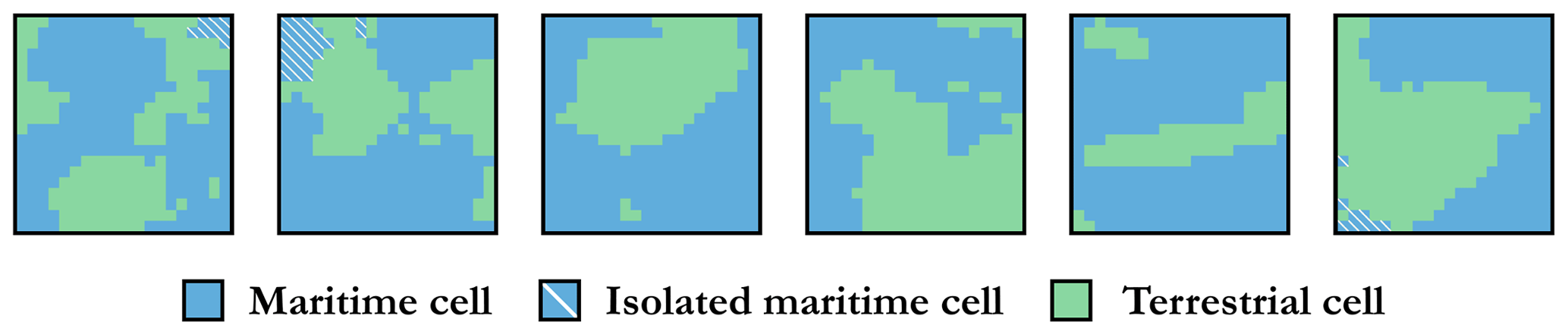
Figure 22 Examples of instances (n=15) withdrawn from the catalogue due to special bottleneck situations.

Figure 23 Organisation of the repository for the catalogue of instances.

5 Data availability

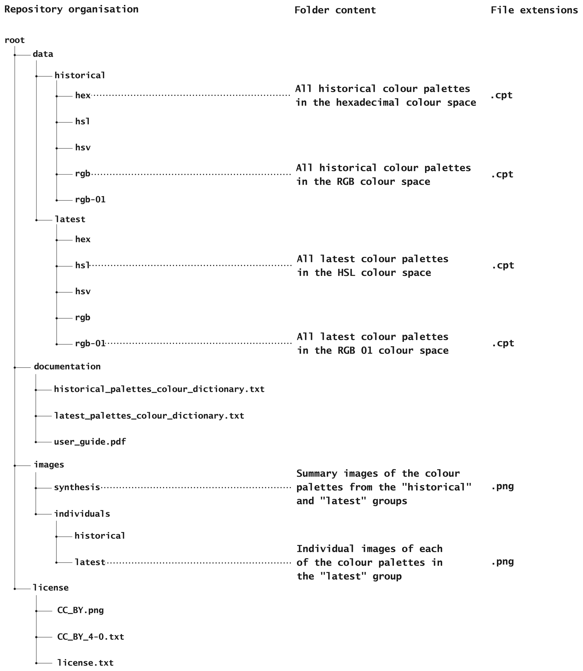
The catalogue produced as part of this research is accessible for download on Zenodo, a general-purpose repository operated by CERN (European Organisation for Nuclear Research) and developed within the European OpenAIRE initiative, at the following persistent link: https://doi.org/10.5281/zenodo.10530247 (Thuillier et al., 2024c). In particular, the repository contains the 17 700 instances supplied in Esri ASCII format, as well as comprehensive documentation, including a user guide detailing the entire dataset and its organisation. In addition to this user guide, we also provide visualisations of the 17 700 instances in the form of duly annotated satellite images and in the form of mosaics made up of two-colour thumbnails, with both Mercator and equirectangular projection. In addition to this catalogue, a set of 18 colour palettes dedicated to the visualisation of DEMs has also been derived for the occasion and is available at the following persistent address: https://doi.org/10.5281/zenodo.10530296 (Thuillier et al., 2024e). This collection of palettes also comes with extensive documentation. The organisation of these two repositories is illustrated in Figs. 23 and 24, respectively.

Figure 24 Organisation of the repository for the colour palettes.

6 Conclusions and perspectives

In this paper, we have provided free access to what is, to the best of our knowledge, the first catalogue consisting of 17 700 coastal instances spread throughout the globe and distributed equally between three libraries, namely A, B, and C. These instances, or digital elevation models (DEMs), are delivered in the form of raster grids with bathymetric and topographic data originating from the General Bathymetric Chart of the Oceans (GEBCO) as of 2022, with a resolution of 15 arcsec, i.e. approximately 460 m × 460 m at equatorial level. These instances cover a wide range of dimensions, from 10 × 10 to 300 × 300, in steps of five (100 instances per dimension for a given library) and a broad spectrum of different coastline geometries. Furthermore, the common feature between these different instances is the presence a unique maritime-connected component with a ratio of maritime cells lying between 25 % and 95 %. These instances are sorted in ascending order in terms of maritime cells within each dimension of a given library. In a nutshell, this catalogue was created with the intention of constituting a reference benchmark for eventual numerical experiments or applications that require working on such areas of interest (AoIs). Moreover, we have provided in-depth details of the automated generation procedure for these instances, and we have proposed a number of visualisations in two and three dimensions and have adapted colour palettes compiled specially for the occasion.

As far as the future is concerned, we can already say that it may be necessary to update this catalogue in a few years' time, once the ocean floor has been mapped more accurately. Indeed, in the period 2022–2023, the scientific consensus is that only 20 % of the oceans have been accurately mapped by direct measurement, with the rest having been interpolated. It would also be interesting to propose an analogous catalogue made up solely of purely maritime instances (i.e. without coastlines) as this could be of interest in many application domains. It would therefore be wise to define criteria to classify these instances and to differentiate them from one another (type of seabed, underwater topography, etc.). Another approach would be to supplement these instances with the GPS coordinates of the various coastlines that we know with greater precision. This could provide additional information compared with the elevation data we currently have at our disposal, the resolution of which can be a hindrance depending on the application being addressed. Finally, it would also be interesting to provide a new library comprised solely of Antarctic instances, which has, so far, been completely excluded from the catalogue.

Appendix A: Coordinate reference system (CRS)

First of all, a CRS, sometimes called a spatial reference system (SRS), enables a point to be uniquely located in a two- or three-dimensional space. There are two main types of CRS: horizontal CRS (2D), used to locate a point on the surface of the globe (i.e. the horizontal component), and vertical CRS (1D), used to give the elevation of a point (i.e. the vertical component). Although a horizontal CRS is essential for defining a point, a vertical CRS is not mandatory. It should be noted that we also refer to a compound coordinate reference system (CCRS) when we combine a horizontal CRS and a vertical CRS (3D).

A1 Horizontal CRS

There are two main types of horizontal CRS: the geographic (geodetic) coordinate system (GCS) and the projected coordinate system (PCS). The former is used to define the location of points on a model (i.e. an approximation) of the Earth's surface, while the latter is planar and necessarily contains a GCS from which the projection is made. In short, the GCS describes where points are on the Earth's surface, and the PCS describes how to represent them on a flat surface (see Fig. A1).

Figure A1 Synthetic difference between a GCS and a PCS.

More specifically, a GCS is made up of the following:

• a reference spheroid or ellipsoid²¹, used to approximate the shape of the Earth;

• a (horizontal) datum used to position the reference spheroid at a certain point relative to the Earth on a so-called anchor point (horizontal reference point)²²;

• a reference meridian to locate the 0° of longitude;

• an angular unit, often degrees (in decimal degrees (DD) or degrees–minutes–seconds (DMS) notation) or even radians, in some cases.

As a reminder, the latitude of a point is the angle formed by the normal to the plane tangent to this point within the equatorial plane. It is an angular value expressing the north or south position of a given point (relative to the Equator). The longitude of a point corresponds to the angle at the centre that the plane passing through this point and through the Earth's axis of rotation forms with the plane of the reference meridian (i.e. prime meridian). It is an angular value expressing the east or west position (relative to the prime meridian). See Fig. A2 for a visual explanation. A GCS is therefore based on these imaginary lines of latitude (parallels) and longitude (meridians), which are structured into a so-called graticule to enable all the points on Earth to be identified (with respect to a given spheroid and a datum), as illustrated in Fig. A3.

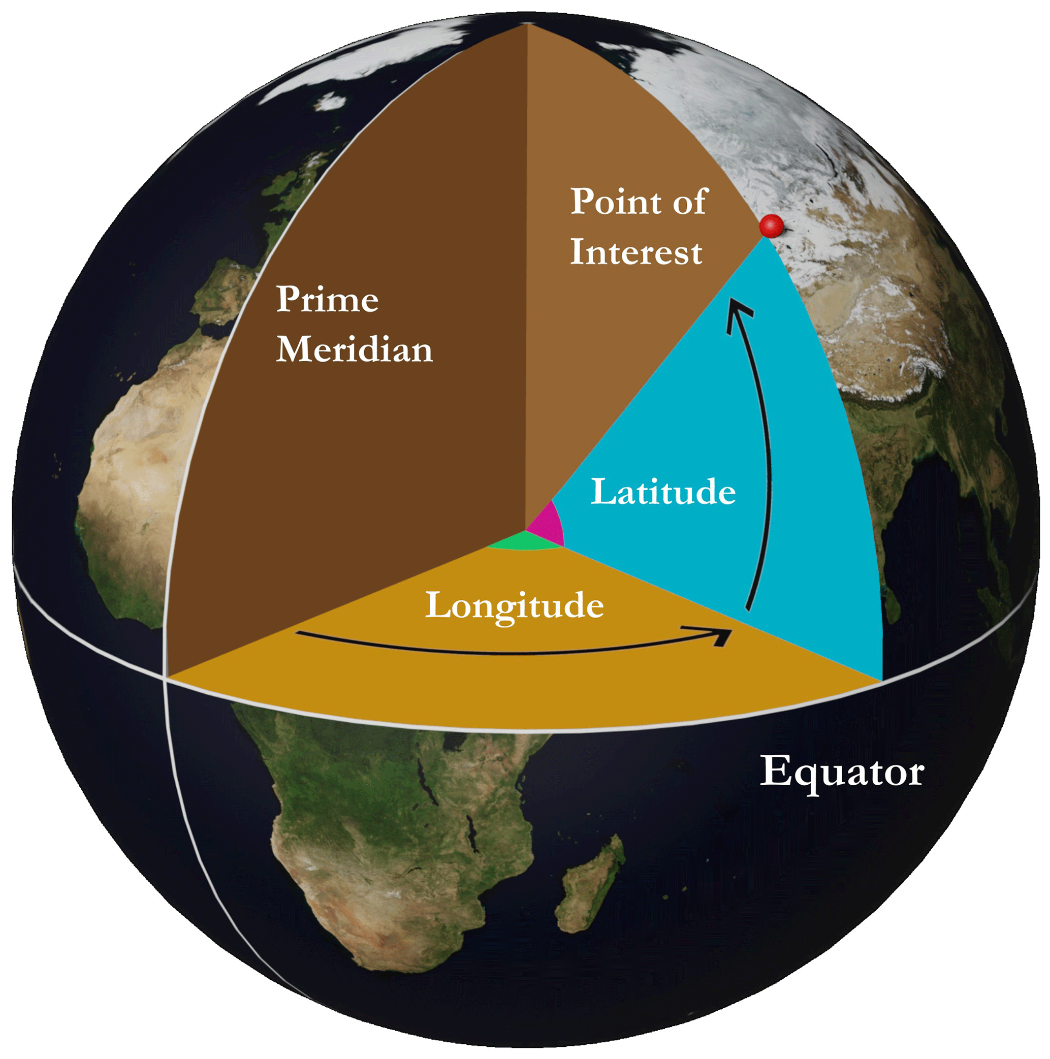
Figure A2 Latitude and longitude: a visual interpretation.

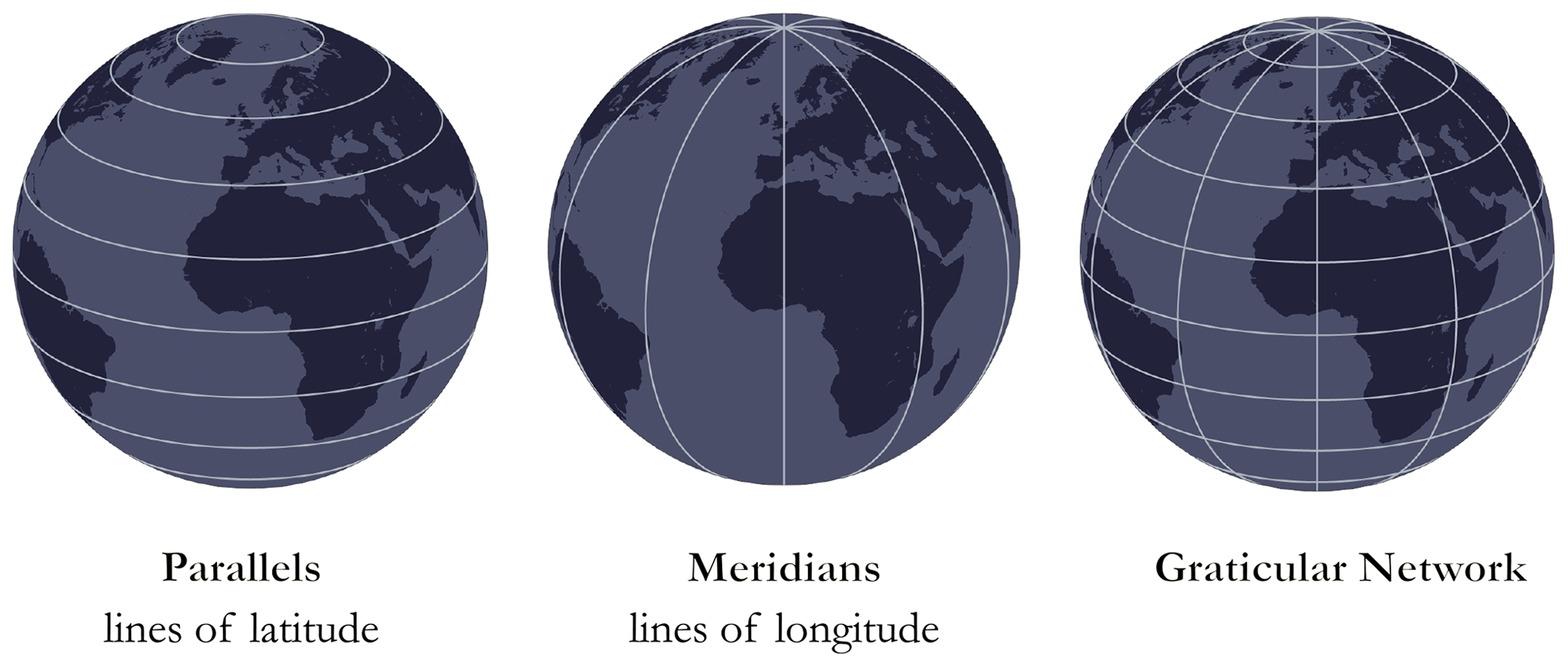
Figure A3 Illustration of the graticular network made up of imaginary lines known as parallels and meridians.

Given that the Earth is not perfectly round, there is a plethora of datums (spheroid + anchor point) that are more or less adapted to certain parts of the world depending on the reference spheroid on which they are based. Nevertheless, a more accurate representation of the Earth's surface than spheroidal models is the geoid, which corresponds to an equipotential in the Earth's gravity field. More precisely, the geoid is, at all points, perpendicular to the direction of the gravity vector (i.e. the direction of the plumb line). And, as the mass of the Earth is not uniform at all points and because the direction of gravity changes, the shape of the geoid is, thus, irregular (bumpy), which is why it is easier to manipulate spheroids that simply approximate it as closely as possible, either locally or globally (see Fig. A4 for an illustration). In simpler terms, the geoid can be described as the surface that coincides with the undisturbed mean level of the oceans (e.g. without storms and tides), with its imaginary extension going through the continental masses. For a continental mass, the geoid could be physically described at any point by digging a narrow channel to connect it with an ocean, thus causing the water in the channel to settle at the level of the geoid (Lambert, 1926). In particular, there are several geoid models, such as the Earth gravitational models (EGMs) of 1984 (EGM84), 1996 (EGM96), and 2008 (EGM2008). Figure A5 shows a view of the EGM2008 geoid. Back to the spheroids, it is possible to distinguish one from another by the lengths of the semi-major and semi-minor axes. For example, consider Table A1, with four particular spheroids.

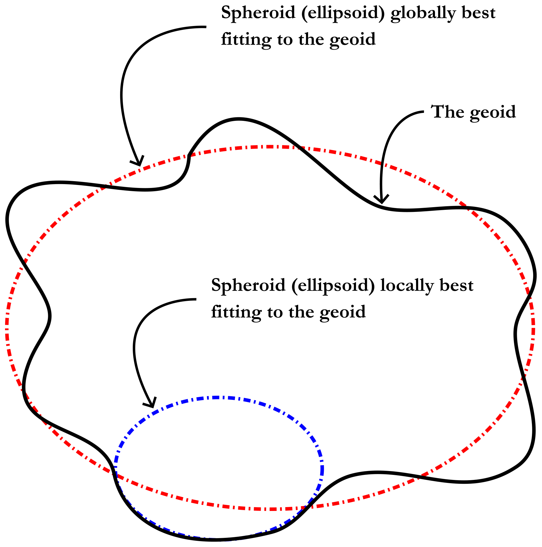
Figure A4 The geoid, the ellipsoid that best fits it at the global level, and the ellipsoid that best fits it at the regional level for a restricted region.

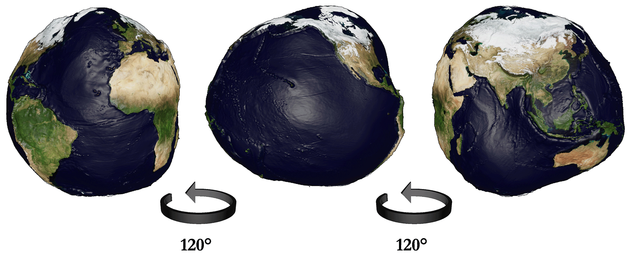
Figure A5 Visualisation of the 2008 Earth gravitational model (EGM2008) geoid with vertical exaggeration and background texture from NASA Visible Earth (Blue Marble: Next Generation, December version).

Table A1 A few examples of spheroids.

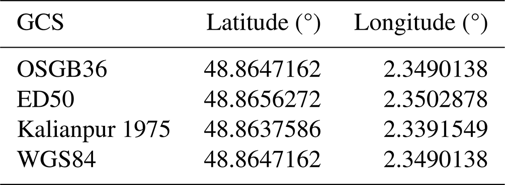
We note that, depending on whether we use the Clarke 1866 spheroid, International 1924 (Hayford), GRS80, or WGS84 to define a datum and, therefore, by extension, a GCS, we will not obtain the same locations for a single point in space. One spheroid may be more suitable than another for a given region because it approximates the geoid for that region as closely as possible (but it may be a poor approximation for another part). The best known is the WGS84 spheroid, which is a reliable global approximation and is therefore used as the standard for the global positioning system (GPS), among other things. It should also be noted that there are some possible confusions as there is the WGS84 GCS based on the WGS84 datum, itself based on the WGS84 spheroid. The WGS84 GCS uses the Greenwich meridian as its reference meridian, and the angular unit is the degree.

Thus, the choice of GCS and, therefore, by extension, of the datum and reference spheroid, is crucial as the coordinates will not be the same depending on the approximation used. An example is shown in Table A2, with the details of the city of Paris in various GCSs.

Table A2 Differences in coordinates for the city of Paris depending on the GCS used.

Now that we know where our points are, and so we can decide to supplement our GCS with a PCS in order to project our points onto a flat surface (i.e. in two dimensions). A PCS is made up as follows:

• a GCS defining the Earth model on which the PCS is based (input details);

• a type of projection, strictly speaking;

• a linear unit such as a metre or a kilometre, for example.

The projection corresponds to the algorithm used to transform the Earth according to the model defined in the GCS into a flat surface (do not confuse projection and PCS; the former is included in the latter). Note that, depending on the projection used, there may be a certain number of additional parameters (e.g. false easting, central meridian, standard parallel) enabling the PCS to be centred on a certain part of the world. Nevertheless, as there is no way to transpose a curved surface (spheroid) into a flat surface without inducing any distortion, there are a multitude of projections with different properties (more than 100 projections). Some projections preserve local angles, and others preserve the surface, while some preserve specific distances or directions. In general, the choice of projection is guided by the extent, location, and property that need to be preserved. Figure A6 shows some reference projections. For the GEBCO grid, as we will see later in Sect. 2, the preferred projection is the flat square projection, which is a special case of an equirectangular projection centred on the Equator.

Figure A6 Some examples of common projections.

Figure A7 Overview of the difference between the two types of vertical datum: geometric model (spheroid or ellipsoid) and gravity-related model (geoid).

A2 Vertical CRS

There are the vertical CRS, which can be coupled with various horizontal CRS to create a complete 3D system (i.e. elevation included). The Geodetic Glossary (2009) defines elevation²³ as “the distance, measured along a perpendicular, between a point and a reference surface”. Although this definition is precise and concise, it leaves some ambiguity with regard to the reference surface used, which is an essential element of a vertical CRS. A vertical CRS, sometimes called a VCS (vertical coordinate system), is formally made up of the following:

• a datum or vertical datum representing the reference point (surface) from which to measure an elevation (depth or altitude) – this is the zero-point of elevation (note that there are two main types of VCS, namely those based on geometric models (ellipsoidal, spheroidal), which are referred to as datum (similarly to those in the horizontal CRS), and those based on gravity-related models (geoidal), which are referred to as vertical datum);

• a direction for the main axis, which can be directed upwards or downwards depending on the quantity being measured (height or depth);

• a unit of measurement, necessarily linear, such as a metre or a foot.

In the case of a VCS based on a geometric model, the elevations are measured directly from a reference spheroid (e.g. the WGS84 spheroid), whereas, in the case of a gravity-related model, the elevations are measured from a geoid (e.g. Earth gravitational model (EGM) 2008) or an approximation thereof. It should be noted that mean sea level (MSL) has long been considered to be a satisfactory approximation in relation to the geoid and can therefore be used as a reference surface for determining elevation. Nowadays, we know that the mean sea level can deviate from the geoid by 1 m, but the exact difference is proving to be difficult to determine. Despite this, much of the data are still referenced to MSL. At its simplest, the MSL corresponds to the average position of the ocean surface measured over time. The aim is to minimise, as far as possible, the random and periodic variations caused, for example, by tides or storm surges. The time window for measuring these variations in the ocean surface has been set at 19 years by the US National Ocean Surface. These measurements can then be combined to form various tidal data such as (in addition to MSL) the mean low water (MLW), the mean tide level (MTL), or even the mean lower low water (MLLW), among many others. Nevertheless, in this form, the MSL is not necessarily the most suitable global vertical reference as this computation only exists at a given measuring station and in its immediate vicinity (e.g. the Marseille tide gauge used to measure elevation in France). There is also a point to be borne in mind when coupling a VCS with a horizontal CRS if one wishes to use a geometric model for the elevation: care must be taken to ensure that the reference spheroid is identical for the VCS and the GCS (or the PCS, if applicable). These different types of information are summarised in Fig. A7.

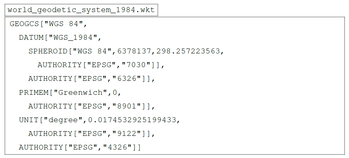
A3 Unique reference code: European Petroleum Survey Group (EPSG)

The EPSG Geodetic Parameter Dataset is a register of spheroids, data, horizontal and vertical CRS, units, etc. This register was initiated by the European Petroleum Survey Group (EPSG) in 1985 and assigns to each feature an EPSG code between 1024 and 32767, as well as a textual (human-readable) description in the “well-known text representation of coordinate reference systems (WKT or WKT-CRS)” format. The register is currently maintained by the International Association of Oil & Gas Producers (IOGP) Committee. These EPSG codes are used extensively in GIS software. For example, the WGS84 horizontal CRS is identified by EPSG:4326, while the WGS84 spheroid is identified by EPSG:7030, and the WGS84 datum is identified by EPSG:6326. For vertical CRS based on MSL, we find, for example, MSL height with EPSG:5714 (positive upwards) or MSL depth with EPSG:5715 (positive downwards). The content of a file in the WKT format for the WGS 84 CRS is shown below.

Appendix B: Digital elevation model (DEM)

A digital elevation model (DEM) is a three-dimensional approximation of a terrain surface by means of a discrete set of points (3D) or point clouds, expressed according to a horizontal CRS (2D), and to which an elevation is associated, expressed according to a vertical CRS (1D) (see Appendix A for the definition of these CRS) (Hirt, 2014). DEMs are digital in the sense that they are produced, distributed, and used in a digital format (Croneborg et al., 2020), and they are models because the elevations must be available at all points in the AoI (Pike et al., 2009; Hengl and Evans, 2009; Szypuła, 2017). Indeed, if the elevation is not available at every point then these are simply samples of heights at discrete locations (points or lines such as contour lines) and not models of a land surface (Hengl and Evans, 2009). It should also be noted that a DEM can represent the dry-land surface (topography) and/or submerged surfaces (bathymetry) of the surface of a terrestrial area (Earth-based), as well as that or those of solid celestial bodies such as asteroids, satellites, or planets (telluric or gaseous) (Guth et al., 2021). In addition, when a DEM covers an entire area, such as the Earth's surface, it is also referred to as a discrete global grid (DGG), as is the case with the GEBCO global grid (see Sect. 2). More specifically, DGGs are a partitioning of space, i.e. a division into non-overlapping regions (e.g. pixels): a mosaic. Sometimes, DEMs are also referred to as “2.5D” rather than true 3D models as some terrain features (e.g. caves and overhanging cliffs) cannot be properly represented (Hirt, 2014).

In the literature, a DEM is often used as an umbrella term for either a digital surface model (DSM) or a digital terrain model (DTM) without further information about the surface (Masini et al., 2011a; Hirt, 2014; Guth et al., 2021). A DSM takes into account all the objects and structures present on the ground, whether they belong to the biosphere (vegetation) or the anthroposphere, i.e. all human-made structures (e.g. power lines, buildings, bridges) (Hirt, 2014; Guth et al., 2021). A DTM filters out the biosphere and anthroposphere, leaving only a representation of the bare ground (bare Earth surface) (Hirt, 2014; Guth et al., 2021). In other words, a DSM corresponds to the highest surface (radar reflective), while the DTM is a DSM stripped of all surface objects, either natural or human-made. The difference between these terms is illustrated schematically in Fig. B1. It should be noted, however, that there is no consensus on the definition of the terms DEM, DTM, and DSM in the scientific literature (Hirt, 2014). Thus, sometimes, DEM and DTM are used as synonyms (Arundel et al., 2015; Croneborg et al., 2020) or DEM and DSM are used as synonyms (Graham et al., 2007), or DEM is defined as a subset²⁴ of a DTM (Zhou, 2017). As in Sect. 2, although we call the GEBCO global grid a DEM, it would be entirely possible and appropriate to call it a DTM as it is more precise.

Figure B1 Differences between a DSM and a DTM.

Going further, according to Hengl and Evans (2009), all DEMs can be classified into the following two groups (see Fig. B2 for a schematic view of the differences):

• vector-based, or irregular, or

• raster-based (grid-based²⁵), or regular.

Figure B2 The two different types of DEMs: raster-based and vector-based.

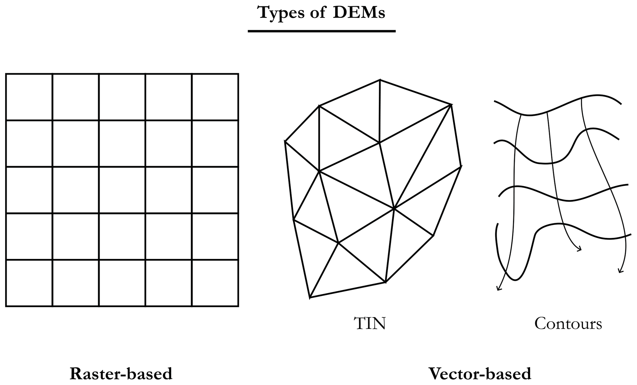
In the vector-based or irregular group, there are two main sub-categories (Masini et al., 2011b): triangular irregular networks (TINs) and contours (level lines). The former involves deriving a DEM using a triangulation algorithm to pave a surface with a set of non-overlapping contiguous triangles (irregulars). This can be done using Delaunay triangulation, where the vertices of each triangle correspond to points in the initial sample and where we try to maximise the minimum of all the angles of the triangles in the triangulation (so as to avoid sliver triangles). In this way, in each triangle, the surface (facet) is represented by a plane between the three vertices, and the values of the points inside can be calculated through interpolation. As for contour-based irregular DEMs, they are derived using lines connecting points of same the elevation, i.e. isohypses (isoheights) and isobaths (isodepths), as well as their orthogonals, in order to produce surfaces (Hengl and Evans, 2009; Masini et al., 2011a). The advantage of these irregular DEMs is that it is possible to accurately capture sudden changes in elevation in the area concerned, with a number of points being equivalent to a DEM in raster form (de Sousa et al., 2006). To be more precise, in Mark (1975), the author was one of the first to compare TINs with DEMs in raster form and to conclude that it took twice as much memory to obtain as good an estimate as with TINs using DEMs. The major drawback is that it is difficult to manipulate DEMs in these vector forms compared with the raster DEMs presented thereafter.

The raster-based or regular group includes DEMs based on regular tiling (i.e. a grid) of space using polygons such as triangles, squares, or hexagons²⁶, the only regular shapes that can be used to tile (tesselate) a given space (i.e. no overlaps or gaps). In this group, the DEMs are then stored in the form of a matrix whose values correspond to the elevations. The advantages of this regular tiling of space are that the conversion between the coordinates of a geographic point in a given CRS and the coordinates of the corresponding pixel in the matrix is trivial, and the structure is simple enough to permit visualisation.

Overall, there is only one important characteristic for this type of DEM: the size of a cell (pixel), which defines the so-called resolution of the DEM. In addition, because of their ease of use, models based on a regular tiling of space using squares remain a standard for DEMs (see, in particular, Sect. 2). However, the major disadvantage of raster DEMs is that they tend to under-sample areas with complex topography and over-sample areas with less complex (i.e. smooth) topography due to the regular spacing of the polygons. Unlike vector models such as TINs or contour-based DEMs, abrupt changes in elevation are not particularly well described using raster DEMs.

It should also be noted that the grid of a DEM does not necessarily have to be regular and stored in the form of a two-dimensional array (matrix); it can be irregular and stored using quadtrees, for example. Similarly, vector-based DEMs can be regular, for example, and as stated in Hengl and Evans (2009), a regular lattice of points stored as a vector layer is regular. The regular–irregular distinction for DEMs can therefore be a source of confusion, and it is better to retain the notion of rasters or vectors for DEMs (Hengl and Evans, 2009).