Enhancing long-term vegetation monitoring in Australia: a new approach for harmonising the Advanced Very High Resolution Radiometer normalised-difference vegetation (NVDI) with MODIS NDVI

Long-term, reliable datasets of satellite-based vegetation condition are essential for understanding terrestrial ecosystem responses to global environmental change, particularly in Australia, which is characterised by diverse ecosystems and strong interannual climate variability. We comprehensively evaluate several existing global Advanced Very High Resolution Radiometer (AVHRR) normalised-difference vegetation index (NDVI) products for their suitability for long-term vegetation monitoring in Australia. Comparisons with the MODIS NDVI highlight significant deficiencies, particularly over densely vegetated regions. Moreover, all the assessed products failed to adequately reproduce the interannual variability in the pre-MODIS era as indicated by Landsat NDVI anomalies. To address these limitations, we propose a new approach to calibrating and harmonising NOAA's Climate Data Record of AVHRR NDVI to the MODIS MCD43A4 NDVI for Australia using a gradient-boosting decision tree ensemble method. Two versions of the datasets are developed, one incorporating climate data in the predictors (“AusENDVI-clim”: Australian Empirical NDVI-climate) and another that is independent of climate data (“AusENDVI-noclim”). These datasets, spanning 1982–2013 at a spatial resolution of 0.05° and with a monthly time step, exhibit strong correlations (r²=0.89–0.94) and low mean errors compared with MODIS MCD43A4 NDVI (mean absolute error (MAE) = 0.014–0.028, RMSE = 0.021–0.046), accurately reproducing seasonal cycles over densely vegetated regions. Furthermore, they closely replicate the interannual variability in vegetation condition in the pre-MODIS era. A reliable method for gap-filling the AusENDVI record is also developed that leverages climate, atmospheric CO₂ concentration, and woody-cover fraction predictors. The resulting synthetic NDVI dataset shows excellent agreement with the MODIS MCD43A4 NDVI and the recalibrated AVHRR NDVI time series (r²=0.82–0.95, MAE = 0.016–0.029, RMSE = 0.039–0.041). Finally, we provide a complete 41-year dataset where the gap-filled AusENDVI-clim from January 1982 to February 2000 is joined with the MODIS MCD43A4 NDVI from March 2000 to December 2022. Analysing 40-year per-pixel trends in Australia's annual maximum NDVI revealed increasing values, and shifts in the timing, of the annual peak NDVI across most of the continent, underscoring the dataset's potential to address crucial questions regarding the changing vegetation phenology and its drivers. The AusENDVI dataset can be used for studying Australia's changing vegetation dynamics and downstream impacts on the terrestrial carbon and water cycles, and it provides a reliable foundation for further research into the drivers of vegetation change. AusENDVI is open access and available at https://doi.org/10.5281/zenodo.10802703 (Burton et al., 2024).

1 Introduction

Australia is undergoing long-term changes to its climate that are impacting terrestrial vegetation, with attendant serious implications for ecosystem functioning, the carbon and water cycles, and agriculture (Hoffmann et al., 2019; Canadell et al., 2021; Head et al., 2014; Hughes, 2011; Steffen et al., 2011; Rifai et al., 2022; Ukkola et al., 2016; Donohue et al., 2009). Long-term, reliable datasets that chart the land surface response to climate change are crucial if we are to identify, understand, and respond to ongoing terrestrial ecosystem change (Giglio and Roy, 2020; Piao et al., 2019). One of the primary means that Earth system science has to trace long-term vegetation change is the normalised-difference vegetation index (NDVI), a widely used satellite-derived indicator of vegetation condition owing to its close relation to vegetation productivity. In Australia, the need for very long records of NDVI to understand change is amplified by strong variability at both interannual and interdecadal timescales and ecosystems that are often driven by periodic but non-seasonal phenological drivers (Moore et al., 2016; Chambers et al., 2013; Ma et al., 2013; Beringer et al., 2022).

Table 1 Details of the datasets used in, and produced by, this study.

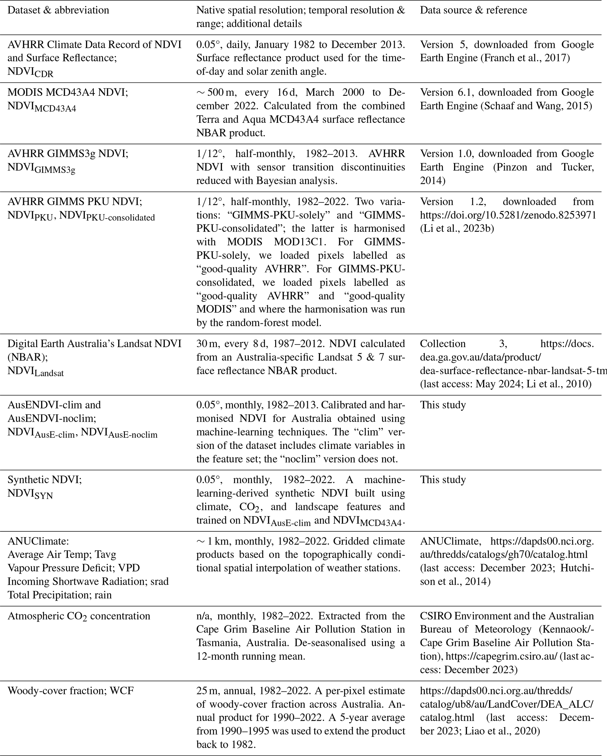
n/a: not applicable

The MODerate resolution Imaging Spectroradiometer (MODIS) NDVI record (NDVI_MODIS) is generally considered the most reliable global-scale dataset due to its high-quality radiometrics and accurate georeferencing. Unfortunately, the MODIS record only begins in March 2000 (Vermote et al., 2002). The Advanced Very High Resolution Radiometer (AVHRR) NDVI record (NDVI_AVHRR) is the longest contiguous series of satellite data, starting in July 1981, but it has several well-known problems owing to a lack of on-board calibration for visible wavelengths, sensor orbital drift, and sensor degradation, making it unreliable for detecting relatively subtle trends over multiple decades (Tucker et al., 2005; Privette et al., 1995; Gorman and McGregor, 1994). Several prominent global NDVI_AVHRR products attempt to ameliorate these issues. For example, the Global Inventory Modelling and Mapping Studies (GIMMS) version 3 (NDVI_GIMMS3g) applies Bayesian analysis with the Sea-Viewing Wide Field-of-View Sensor NDVI as evidence information to reduce sensor transition discontinuities and increase the dynamic range of NDVI_AVHRR (Pinzon and Tucker, 2014), while the NOAA Climate Data Record (NDVI_CDR) applies a suite of corrections to create a consistent surface reflectance product (Franch et al., 2017), among others (Table 1). However, despite substantial progress, errors and biases in these NDVI products have led to inconsistent findings on global greening (Wang et al., 2022, 2021; Cortés et al., 2021; Frankenberg et al., 2021; Fensholt and Proud, 2012), discrepancies in vegetation seasonality between datasets (Ye et al., 2021), persistent temporal inconsistencies (Tian et al., 2015; Giglio and Roy, 2020), and conflicting long-term trends in the interannual variability of vegetation greenness (Tian and Luo, 2024). Recently, Li et al. (2023a) developed new global NDVI_AVHRR products: “GIMMS-PKU” (NDVI_GIMMS-PKU), which effectively calibrates the NDVI_GIMMS3g archive to the Landsat record using machine-learning techniques; and “GIMMS-PKU-consolidated” (NDVI_{PKU-consolidated}), which harmonises NDVI_GIMMS-PKU to NDVI_MODIS (Table 1) but is yet to be extensively assessed in the literature (Li et al., 2023a).

As much as possible, any NDVI product that exploits the AVHRR and MODIS records to acquire an accurate >40-year record of vegetation condition should attempt to integrate the two seamlessly while also performing well in the pre-MODIS AVHRR era (1982–2000). Performance should be judged on how well seasonal cycles are represented along with interannual and interdecadal variability, as both seasonal and longer-term fluctuations in vegetation conditions have important ramifications for carbon and water cycles (Ma et al., 2015). An effectively calibrated, harmonised, and gap-filled dataset can form the basis for studying the biogeophysical impacts of global change and meteorological variability on Australia's terrestrial vegetation. With that in mind, the objectives of this study are as follows:

• Investigate existing NDVI_AVHRR datasets to determine their suitability for long-term vegetation monitoring in Australia by comparing their consistency with both NDVI_MODIS during the 2000–2013 overlap period and Landsat NDVI (NDVI_Landsat) anomalies from 1988–2000.

• Having established the limitations with the existing datasets, calibrate and harmonise NDVI_AVHRR to NDVI_MODIS solely over Australia. The final dataset should contain the harmonised NDVI_AVHRR from January 1982 to February 2000, where it joins with the superior NDVI_MODIS time series, resulting in a reliable 41-year record of vegetation condition for Australia. We will call this time series “AusENDVI” (for Australian Empirical NDVI; NDVI_AusE).

• Develop a reliable method for gap-filling the NDVI_AusE record caused by sensor transition issues and long periods of missing or suspect data acquisition.

• Demonstrate the utility of this new dataset by exploring NDVI phenology trend analysis, including long-term trends in the value and timing of the annual maximum NDVI across the Australian continent.

2 Materials and methods

2.1 Datasets

Specifications of all datasets used for either the intercomparison of NDVI products or in the modelling framework are listed in Table 1. For comparisons between NDVI datasets, finer-resolution datasets were resampled to match the coarsest grid (i.e. GIMMS; 1/12° or ∼ 8 km over Australia). Averaging resampling techniques were used for downsampling finer-resolution datasets, while nearest-neighbour techniques were used when the datasets had similar spatial resolutions but either different projections or slightly different grid extents. Wherever datasets were compared, data gaps were matched between all datasets by creating a mask that identified all missing pixels, and then that common mask was applied to every dataset. This ensured a fair and valid comparison. We chose Landsat's TM and ETM+ (Table 1) as the sensors for comparison in the pre-MODIS era owing to the international efforts to produce a relatively high geometric and radiometric accuracy for their generation and the lack of sensor transitions in the pre-MODIS era from 1982–1999 (Beck et al., 2011). The chosen surface reflectance Landsat product, Digital Earth Australia's (DEA's) Landsat NBAR (Nadir-corrected BRDF Adjusted Reflectance, where “BRDF” stands for “bidirectional reflectance distribution function”) product is calibrated to Australia's environment using the MODTRAN 4 radiative-transfer model and BRDF shape functions derived from MODIS (Li et al., 2010; Byrne et al., 2024).

For the development of the Australian NDVI dataset, we relied on the NOAA NDVI_CDR product (Franch et al., 2017) as the input dataset. This was principally because of its higher spatial resolution than the other datasets (∼5 km), its lack of gap filling, extensive atmospheric corrections, and its BRDF-based correction of view-angle effects (Ma et al., 2019). As the target dataset, we derived the NDVI from the MODIS MCD43A4 surface reflectance NBAR product (NDVI_MCD43A4). This reflectance product was chosen because of its similar set of atmospheric corrections when compared with NDVI_CDR and DEA's Landsat NBAR and its use of both the Terra and Aqua instruments, which extends its temporal extent back to March 2000 (Schaaf and Wang, 2015).

All additional input data used in NDVI estimation were temporally aggregated to monthly values by calculating medians and spatially reprojected onto a common 0.05° geographic grid. In addition to filtering based on the quality assurance band (we filtered for clouds, cloud shadows, and invalid BRDF and channel values), additional criteria were applied to minimise the impact of temporal discontinuities in the NDVI_CDR record, which may arise from orbital decay or sensor degradation. Monthly NDVI_CDR values based on fewer than two observations per month were discarded along with any values for which the coefficient of variation in daily retrievals for a given month was greater than 50 %. Anomalies in NDVI, solar zenith angle, and time of acquisition that were greater than 3.5 standard deviations were also discarded (based on a 1982–2013 climatology). Following the advice of Tian et al. (2015), data for several problematic sensor transition periods were discarded (September 1984–April 1985, July 1988–September 1989, and July 1993–December 1994). After filtering, the continental-average fraction of available data is 0.79, meaning that, on average, 79 % of the monthly time steps between 1982–2013 are preserved (Fig. A1).

2.2 Assessment of existing NDVI products

We compared NDVI_AVHRR datasets with NDVI_MCD43A4 for the overlapping period from March 2000 to December 2013. The per-pixel Pearson correlation (r) and coefficient of variation (CV; root mean square error divided by the long-term mean NDVI_MCD43A4) were used to describe the agreement between datasets, in addition to a comparison of the long-term seasonal cycles. Next, NDVI_AVHRR datasets were compared to annual rolling-mean “z-score” standardised anomalies in NDVI_Landsat for 1988–2000 to assess how well each product reproduces the interannual variability in vegetation condition in the pre-MODIS era. z-score standardised anomalies were calculated as $(x-\mathit{\mu })/\mathit{\sigma }$, where x is a monthly NDVI observation, μ is the long-term mean NDVI for the given month, and σ is the long-term standard deviation in NDVI for the given month. Differences in spectral sampling between MODIS and Landsat result in differences in mean NDVI, so we use Landsat only for validating the interannual variability in the pre-MODIS era since mean differences in NDVI between sensors are removed by anomalies. We compared NDVI anomalies in NDVI_Landsat with NDVI_MCD43A4 during an overlap period from 2000–2012 to ensure that NDVI_Landsat could provide a consistent evaluation of interannual variability in the pre-MODIS era, and we found good agreement between the two products (Fig. A2).

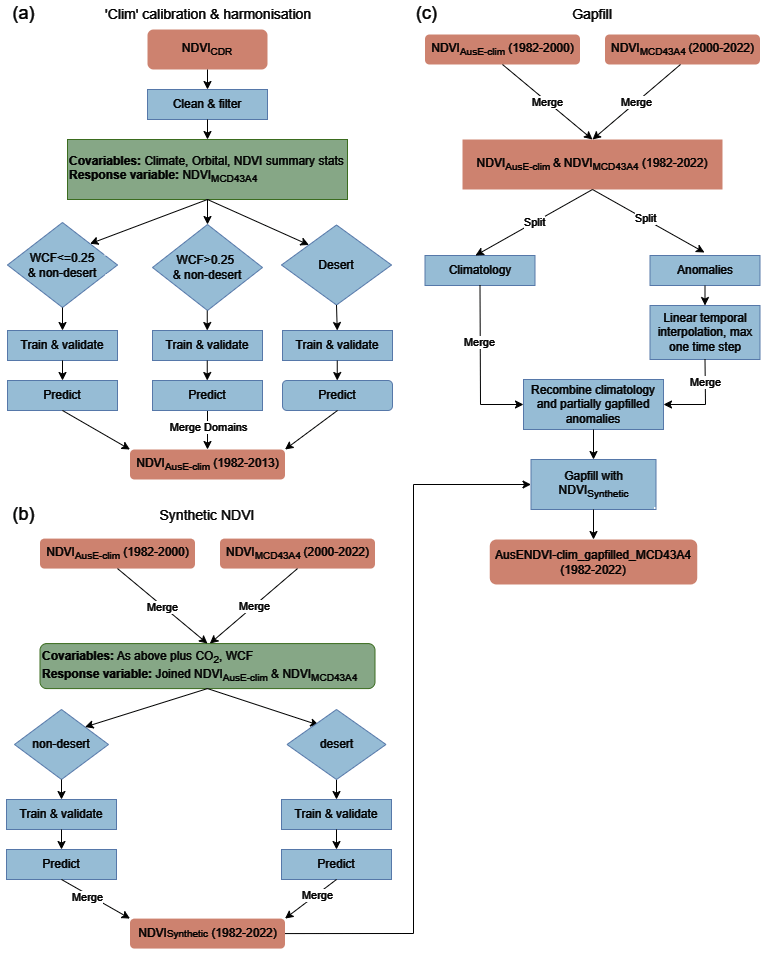
Figure 1 Flowchart describing the calibration and harmonisation methods (a) and the development of a synthetic NDVI (b) for gap filling (c). Panel (a) shows the method for the clim model type; the methods for noclim are the same, but climate variables are removed from the covariables and noclim is not gap-filled. Red-coloured boxes denote datasets, blue boxes denote processing steps, and green boxes describe the response variables and covariables used for modelling.

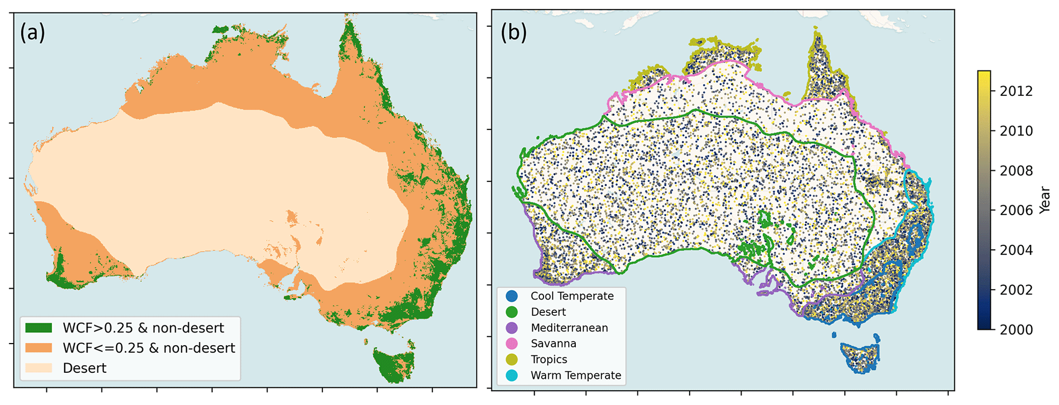
Figure 2 (a) Regions delineating the spatial extents of the three modelling domains: desert, low woody-cover fraction (WCF), and high WCF. (b) The distribution of all independent validation points used to assess the model fits across the three modelling domains in (a); points are coloured according to the year they are drawn from. The figure is overlaid with outlines of the six bioclimatic regions used to both stratify training points and aggregate trends in later analysis.

2.3 Calibration and harmonisation

During extensive preliminary testing, gradient-boosting decision tree ensembles (GBM), random forest, and generalised additive models were assessed for their ability to calibrate and harmonise NDVI_CDR with NDVI_MCD43A4. The GBM outperformed the other approaches. Two classes of models and datasets were built. One utilised climate data (hereafter referred to as “clim” models) in the feature set to achieve the best possible agreement between NDVI_CDR and NDVI_MCD43A4. The second excluded climate features (hereafter the “noclim” model) while still achieving satisfactory results. When examining drivers of change, users of these datasets may prefer to use the noclim model to limit potential circularities in the attribution of the drivers of change. During testing, climate variables were identified as useful features for both improving predictions in the heavily forested regions where there was little to no agreement between NDVI_MCD43A4 and NDVI_AVHRR and for capturing interannual variability. The noclim models used the following features: solar zenith angle (SZEN), time of acquisition (TOD), month of year, latitude, and NDVI_MCD43A4 summary percentiles (0.05, 0.5, and 0.95). The NDVI_MCD43A4 summary percentiles were calculated per pixel over the 2000–2022 period. The clim models used the same variables plus incoming solar radiation, rainfall, temperature, and vapour pressure deficit. Fractional anomalies of the climate features were also included, along with the cumulative 3- and 6-month rainfall. Testing revealed that the best results were obtained by generating three separate models for areas with high and low woody-cover fractions (WCFs) and for the desert bioclimatic region (Figs. 1a and 2a). The long-term mean of the WCF was extracted from Liao et al. (2020), and a threshold of WCF = 0.25 was used to separate regions with high woody canopy cover. This threshold was chosen as it approximately delineated those regions with the poorest correspondence between NDVI_CDR and NDVI_MCD43A4 (Fig. 3e–h).

Owing to the differing volumes of good-quality data across the continent (Fig. A1) and the large difference between the land areas of the bioclimatic regions, we implemented a stratified, equalised random sampling approach for the training and validation samples to reduce bias in the sample allocations. In the high- and low-WCF regions, 30 000 training and testing samples were extracted in equal measure from the five remaining bioclimatic regions after excluding the desert (i.e. 6000 samples per region). The bioclimatic regions were identical to those defined by Haverd et al. (2013) (Fig. 2b). In the desert region, samples were drawn using a simple random approach. In all modelling domains, samples were drawn from any point in time across the overlap period, and 5000 samples were randomly separated as an independent validation set, leaving 25 000 samples for training. The calibration and harmonisation process is summarised in the flow chart of Fig. 1a.

Cross-validation for model hyperparameter optimisation was conducted using a nested cross-validation approach with five outer splits and three inner splits (Cawley and Talbot, 2010). The hyperparameter grid search parameters are listed in Table A1. Mean absolute error (MAE), root mean square error (RMSE), and the coefficient of determination (r²) are reported as indicators of the goodness of fit. To understand which explanatory variables most impacted predictions, feature importance plots were produced using the Shapley Additive Explanations (SHAP) Python library (Lundberg, 2017).

2.4 Gap filling

At times, there are long gaps in the AVHRR data acquisition over Australia. For example, 1994 is entirely missing, and during sensor transition periods, the data become unreliable for several months before and after the transition (Tian et al., 2015). Furthermore, owing to the nature of Australia's prevailing weather systems, such as the tropical monsoon, it is not uncommon to have whole geographic regions missing for a given month. This undermines the typical approaches to gap filling that work well when either the temporal gap is short (e.g. temporal interpolation methods using linear or polynomial fits) or the spatial pattern of gaps is quasi-random, such as that caused by scattered cloud cover (when spatial interpolation methods such as nearest neighbour and kriging are used) (Bessenbacher et al., 2022; Shen et al., 2015). Gap filling with a climatology can often mask important interannual variability at key times, such as anomalously high rainfall periods associated with La Niñas, when enhanced cloud cover masks large-scale greening events across Australia's northern tropical savanna. To avoid this, we used well-established machine-learning approaches that have been developed to fill gaps in univariate data (Gerber et al., 2018; Zeng et al., 2014). Here, we develop a two-stage process for gap filling (summarised in Fig. 1b, c). Firstly, to fill short temporal gaps, the time series is split into a climatology series and an anomaly series, and linear temporal interpolation is applied to the anomalies for a maximum of one time step (i.e. 1 month). Longer temporal gaps are replaced with a synthetic NDVI dataset generated using a similar GBM machine-learning method to the harmonisation and described further below.

Synthetic NDVI

Training samples were extracted from NDVI_AusE-clim for 1982–2000 and from NDVI_MCD43A4 for 2000–2022 using a similar sampling approach to that used for harmonisation except that two models are built in this instance: a “desert” model and “non-desert” model. The non-desert model covers the same region as the high- and low-WCF models previously described (the inclusion of WCF in the features reduces the need to define a low- and high-WCF modelling region). GBM models were then fitted using all the features previously listed for the clim model plus the de-seasonalised CO₂ concentration and annual WCF. Otherwise, the modelling framework was the same as for the harmonisation approach (Fig. 1b). The synthetic NDVI datasets (NDVI_SYN) are used to gap-fill the NDVI_AusE-clim record from January 1982 to February 2000. The final gap-filled, calibrated, and harmonised NDVI_AusE-clim dataset is joined with NDVI_MCD43A4. Only the NDVI_AusE-clim dataset is gap-filled; this ensures that the noclim dataset does not contain any climate information in the reconstructed time series.

2.5 Trends in peak-of-season phenology

Annual, per-pixel NDVI land surface phenology statistics were extracted using the “xr_phenology” Python function from the “dea-tools” package (Krause et al., 2021). This analysis focused on two metrics: the NDVI value at the peak of the season (vPOS) and the day of year on which the peak occurs (POS). The input time series was the gap-filled clim dataset, and the time series was first linearly upsampled from monthly to 2-week intervals to increase the temporal resolution of the datasets before the time series was smoothed using a Savitzky–Golay filter with a window length of 11 and a polynomial order of 3. Though we report day of year as the unit for POS, the actual POS could have occurred anytime within a given bi-monthly time step, so DOY values should be considered an approximation.

To avoid applying phenology trend analysis to regions that do not experience regular seasonal variation, we created a mask that removes regions identified as “non-seasonal” using the definitions and methods defined by Moore et al. (2016). Broadly, the mask is created using three inputs: the standard deviation in NDVI anomalies, the long-term mean NDVI, and the standard deviation in the mean seasonal cycle. These three inputs are used to identify regions that experience either low seasonal variability and low NDVI or low seasonal variability and high interannual variability, which largely coincide with the desert bioclimatic region.

Per-pixel linear trends in these phenology metrics were extracted using the Theil–Sen robust-regression approach, and significance was determined using a Mann–Kendall test (significance was defined as α=0.05). Trends summarised over bioclimatic regions were extracted by first calculating a per-pixel robust regression on the phenology statistics and then summarising the trends within a bioclimatic region with kernel density estimation (KDE) plots.

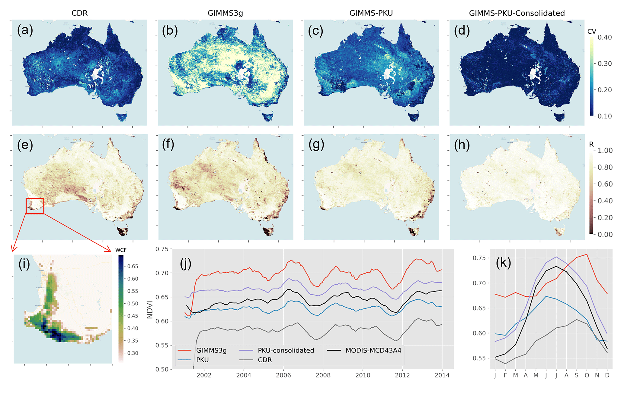
Figure 3 Comparisons between NDVI_MCD43A4 and four versions of NDVI_AVHRR. (a–d) Coefficient of variation (CV) between NDVI_MCD43A4 and NDVI_AVHRR, where RMSE is divided by the 2001–2013 mean of NDVI_MCD43A4. (e–h) Pearson correlation between NDVI_MCD43A4 and NDVI_AVHRR. (i) Woody-cover fraction (WCF) of the forests in southwestern Western Australia showing the extent used for the zonal time series of (j) and (k). (j) Twelve-month rolling-mean NDVI time series of the forests of southwestern Western Australia. (k) Mean seasonal cycle of the forests of southwestern Western Australia calculated over the 2001–2013 period.

3 Results

3.1 Quality of the existing datasets

The quality of the NDVI_AVHRR products were compared against NDVI_MCD43A4 for the overlapping years 2000–2013. All datasets except NDVI_{PKU-consolidated} perform poorly over regions with perennially high vegetation cover, including wet coastal and highland forest ecosystems, where correlations between NDVI_AVHRR and NDVI_MCD43A4 are close to zero in some regions (Fig. 3e–g). NDVI_CDR and NDVI_GIMMS3g also poorly represent the desert region, with R values as low as ∼0.4–0.5. NDVI_{PKU-consolidated} correlates very well with NDVI_MCD43A4 over most of the continent, with the exception of western Tasmania (Fig. 3h). Coefficients of variation are also high for the NDVI_GIMMS3g and NDVI_PKU datasets across much of the continent, with average values of 0.33 and 0.18, respectively (Fig. 3b, c).

To demonstrate the impact of the discrepancies over densely vegetated ecosystems, Fig. 3j–k presents a zonal time series of the woodlands of southwestern Western Australia. These woodlands have been identified as a region of high endemic biodiversity (Myers et al., 2000; Hopper and Gioia, 2004), they are vulnerable to the effects of long-term climate change, and they are undergoing long-term shifts in climate (O'Donnell et al., 2012; Hughes, 2011; Pitman et al., 2004; Hope et al., 2006). The MODIS-era interannual variability of these forests is shown through a 12-month rolling-mean time series (Fig. 3j), which reveals that all products capture the interannual variability of the MODIS era reasonably well, though the long-term mean NDVI value varies substantially between products. The mean seasonal cycle, shown in Fig. 3k (calculated from 2001–2013), reveals that the seasonal cycle of the forest ecosystem is very poorly represented in three of the four products, while NDVI_{PKU-consolidated} tracks the overall shape of the seasonal cycle well. Discrepancies in seasonality are further highlighted in the per-pixel climatological month-of-maximum-NDVI plots (Fig. A3). Estimates of even this relatively straightforward metric of seasonality are impacted by the choice of dataset, with desert, savanna, and forested regions varying substantially between datasets, sometimes by as much as several months in the case of forested regions in Tasmania and southeastern Australia. The Australia-wide seasonal cycles likewise reveal substantial variation between products (Fig. A3g).

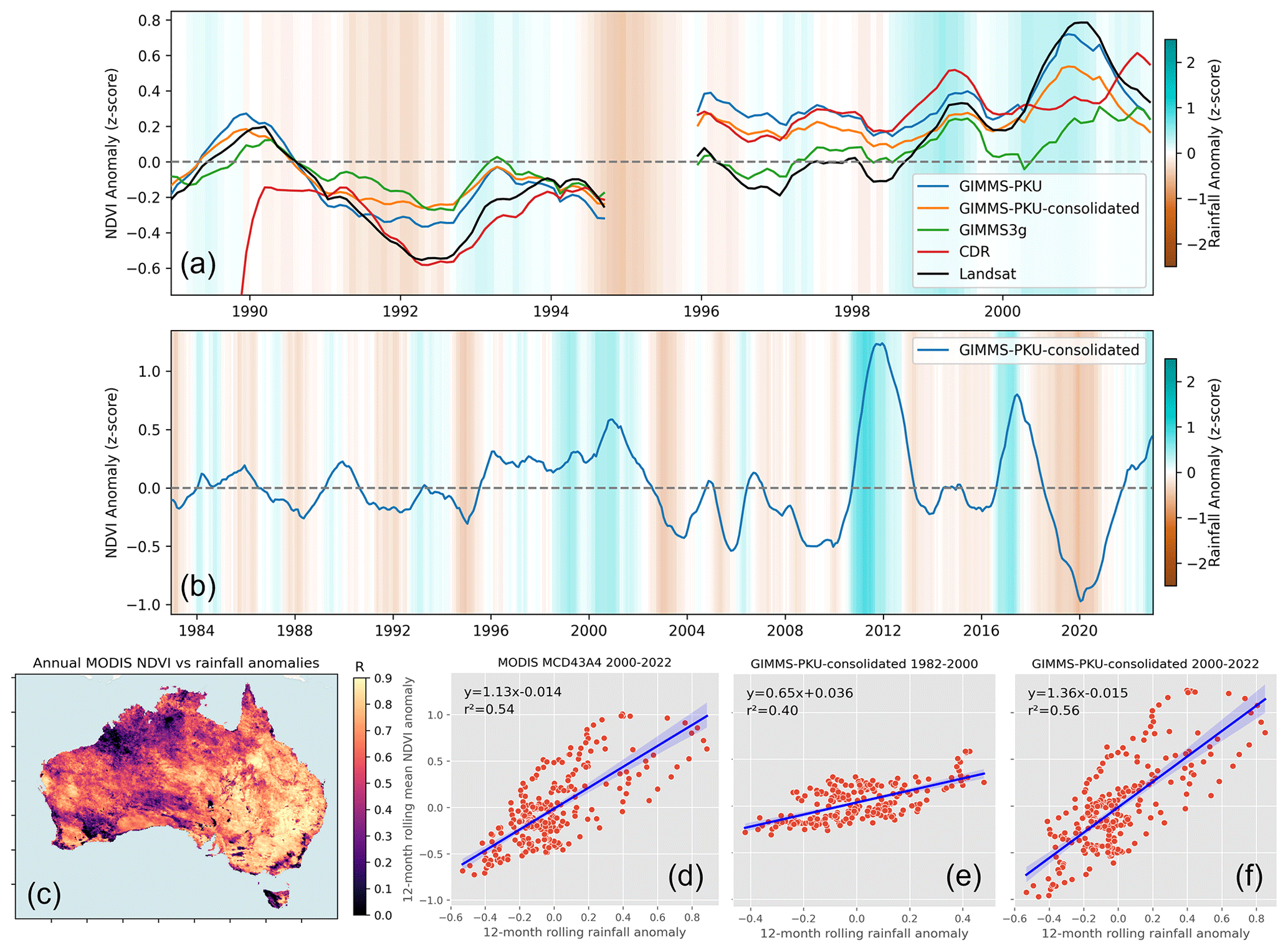
Figure 4 (a) Twelve-month rolling-mean standardised anomalies of the Landsat, CDR, GIMMS3g, GIMMS-PKU, and GIMMS-PKU-consolidated NDVI records, based on a common 1988–2012 climatology. Background shading represents the 12-month rolling-mean standardised rainfall anomalies. All datasets besides rainfall have matching data gaps. (b) Twelve-month rolling-mean standardised anomalies of the NDVI_{PKU-consolidated} product (1982–2022 climatology). (c) Pearson correlations between annual NDVI_MCD43A4 anomalies and annual rainfall anomalies, shown here to demonstrate the strongly water-limited nature of Australia's vegetation. (d–f) Relationships between the 12-month standardised rainfall and NDVI anomalies averaged across Australia for different periods and different products. In (d), the NDVI_MCD43A4 and rainfall anomalies were calculated against the 2000–2022 baseline. In (e)–(f), the rainfall and NDVI_{PKU-consolidated} anomalies were calculated against the 1982–2022 baseline. The relationship $y=mx+c$ denotes the linear regression slope between rainfall and NDVI anomalies, where y is the NDVI anomaly, x is the rainfall anomaly, and m is the slope coefficient. The slope coefficient can be considered an approximation of the sensitivity of NDVI to anomalous water supply aggregated over the continent.

To assess the quality of NDVI_AVHRR products in the pre-MODIS era, Fig. 4a compares the 12-month rolling-mean standardised anomalies of NDVI_Landsat in the 1988–2000 period (based on a 1988–2012 climatology) with the NDVI_AVHRR anomalies. No product accurately tracks the NDVI_Landsat anomalies across the whole 1988–2000 period. Only the NDVI_PKU product captures the amplitude of the La Niña-driven positive anomaly of NDVI in 2000 (but recall that NDVI_PKU is trained on the NDVI_Landsat archive). Annual rainfall and NDVI anomalies are strongly correlated across the majority of Australia's land mass (Fig. 4c), demonstrating that vegetation growth across the continent is strongly water limited (Peters et al., 2021; Poulter et al., 2014; Broich et al., 2014). It is therefore our expectation that similarly large negative and positive rainfall anomalies should result in similar NDVI anomalies in the pre-MODIS and MODIS eras. Taking the best of the products identified in the comparison with NDVI_MCD43A4, Fig. 4b shows the 12-month rolling mean standardised anomalies of NDVI_{PKU-consolidated} from 1982–2022. In the MODIS era, NDVI_{PKU-consolidated} responds strongly to anomalies in rainfall (background shading shows the continental-average standardised rainfall anomalies), while in the pre-MODIS era, significant droughts (e.g. in 1982–1983) and widespread rainfall events (e.g. in 2000) produce comparatively little effect on NDVI, suggesting a lack of sensitivity to rainfall-driven variability over Australia in the pre-MODIS era. We develop statistical relationships between annual-mean standardised rainfall and NDVI anomalies, averaged across Australia, for the NDVI_MCD43A4 and NDVI_{PKU-consolidated} products to quantify their sensitivity to water supply. If we consider the slope of the linear relationship between rainfall and NDVI to be an approximation of the sensitivity of NDVI to water supply, then NDVI_{PKU-consolidated} in the 2000–2022 period displays a similar sensitivity (slope = 1.36; Fig. 4f) and correlation (r²=0.56) to NDVI_MCD43A4 in the same period (slope = 1.13, r²=0.54; Fig. 4d). Contrast this with NDVI_{PKU-consolidated} in the 1982–2000 period, where the apparent sensitivity is approximately half that for the 2000–2022 period (slope = 0.65; Fig. 4e). While we may expect some changes in water-supply sensitivity over the decades due to effects such as CO₂ fertilisation (Donohue et al., 2013; Ukkola et al., 2016), a doubling of annual water supply sensitivity is highly unlikely. Thus, we argue that no current NDVI_AVHRR product currently satisfies our product criteria – that it agrees well with NDVI_MCD43A4 while also producing satisfactory results in the pre-MODIS era.

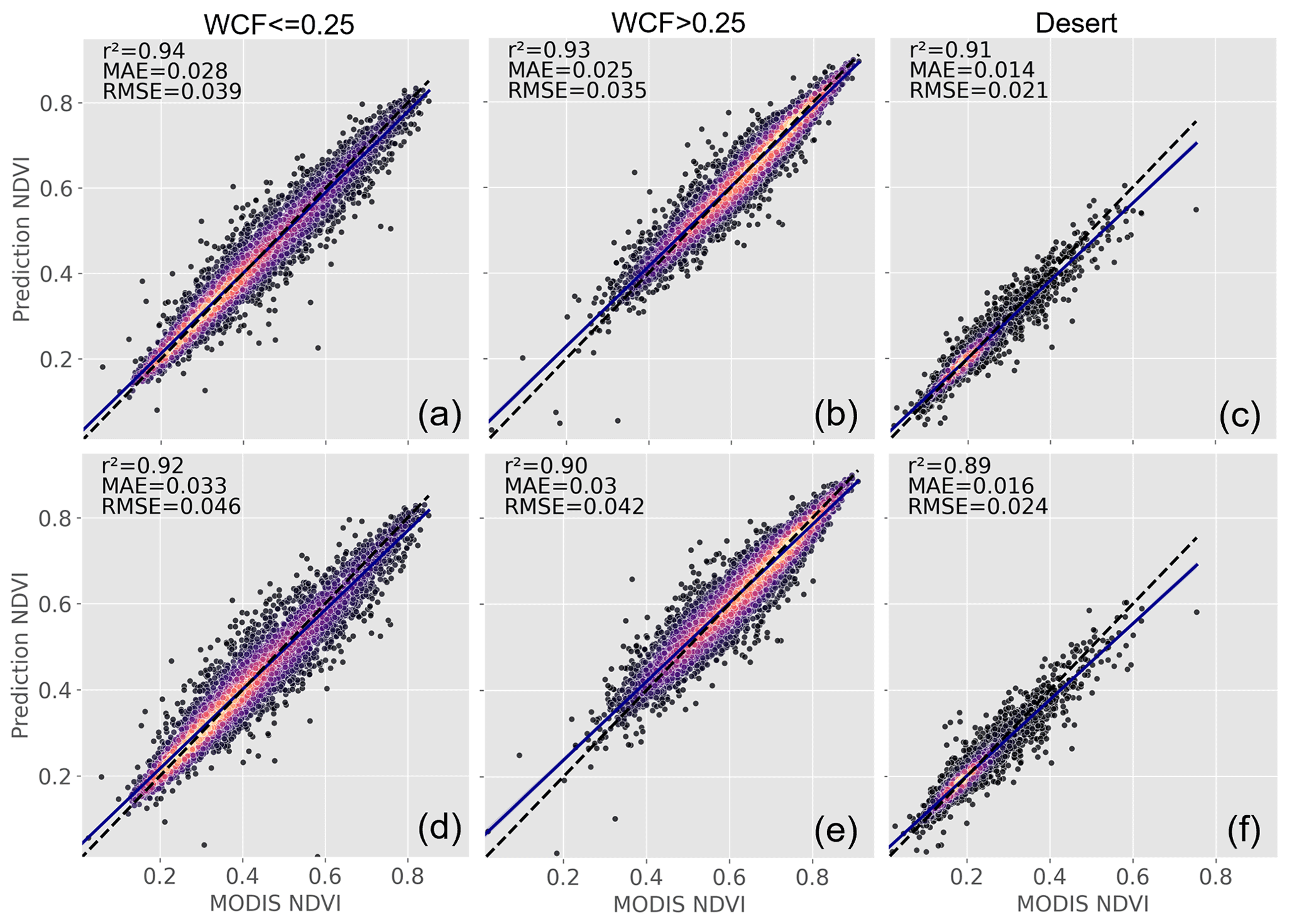
Figure 5 Validation scatter plots for the calibration and harmonisation between NDVI_CDR and NDVI_MCD43A4. Panels (a)–(c) show the results for the clim model. Panels (d)–(f) show the same but for the noclim model type.

3.2 Calibration and harmonisation performance

Independent validation statistics for all six model varieties (clim and noclim; desert and high and low WCF) reveal a high degree of agreement for all model types, with r²≥0.91 for the clim models, RMSE ≤0.039, and MAE ≤0.028 (Fig. 5a–c). The clim model types tended to have errors that were ∼15 % smaller than their noclim counterparts (Fig. 5d–f). SHAP feature importance plots indicate that NDVI_CDR is the most important variable (Fig. A3), but in the high-WCF regions, the relative importance of NDVI_CDR diminished and the NDVI_MCD43A4 summary statistics, solar radiation, and cumulative rainfall substantially impacted predictions (Fig. A4b, c).

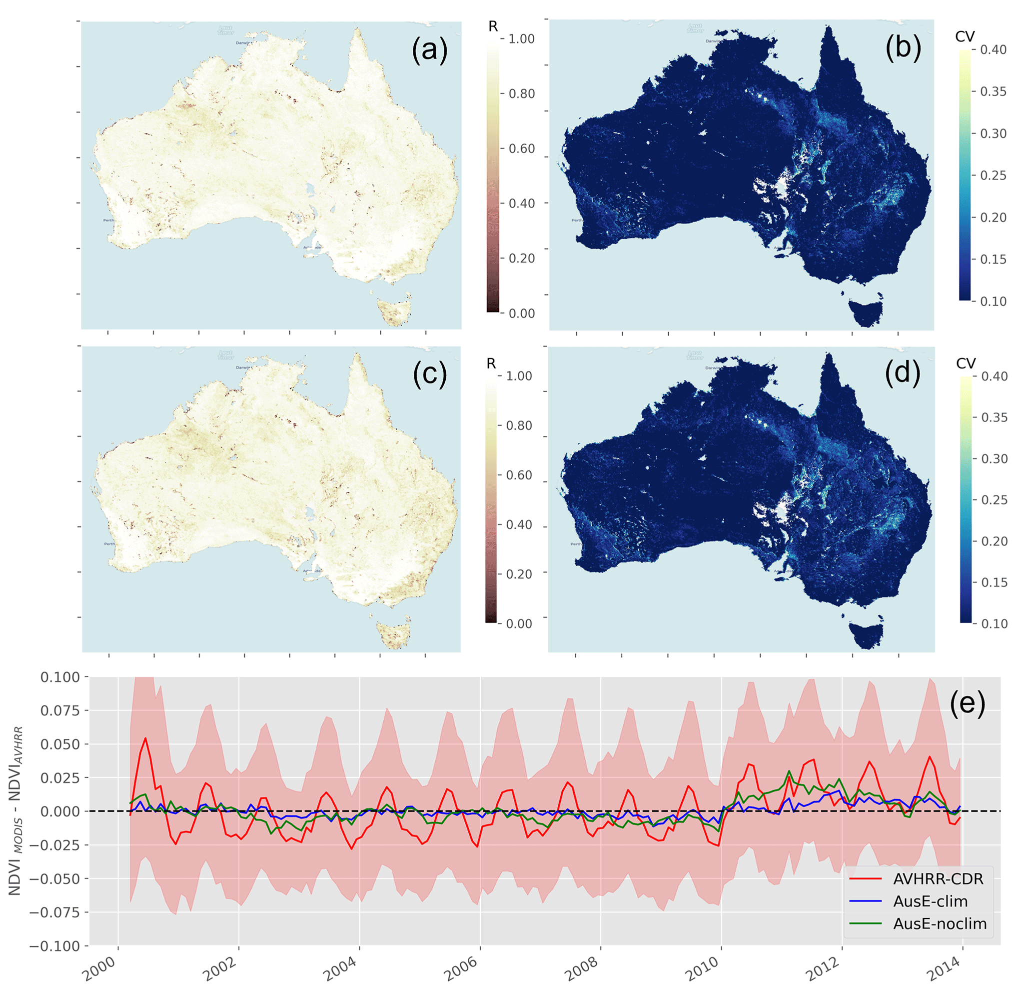
Figure 6 Results of the calibration and harmonisation between NDVI_CDR and NDVI_MCD43A4. Panel (a) shows the per-pixel Pearson correlation between NDVI_MCD43A4 and clim NDVI_AusE. Panel (b) shows the same as (a) but for the coefficient of variation. Panels (c, d) show the same as (a, b) but for the noclim model type. (e) The residual NDVI value when subtracting NDVI_AVHRR from NDVI_MCD43A4 before and after the calibration and harmonisation. Residuals are calculated per pixel and then averaged over Australia. Shading indicates the standard deviation in residuals across the continent for the NDVI_CDR product.

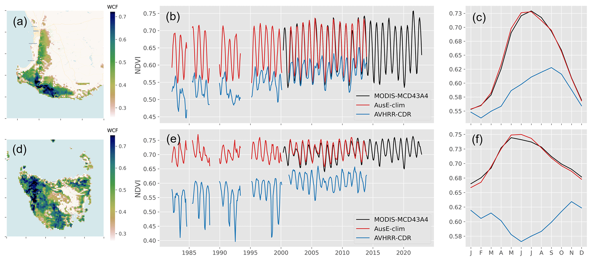
Figure 7 Results before and after the calibration and harmonisation of NDVI_CDR for two examples of regions with high woody canopy cover where NDVI_CDR was previously identified as having the worst agreement with NDVI_MCD43A4. (b, c) Three-month rolling-mean NDVI time series for 1982–2022 and the mean seasonal cycle (averaged over the 2001–2013 period), respectively, for the forests of southwestern Western Australia. (e, f) Same as (b, c) but for Tasmanian forests. The time series are the spatial averages of the regions to their left.

The per-pixel agreement between NDVI_AusE and NDVI_MCD43A4 for both the clim and noclim model types reveals a very high degree of correlation across the continent (note that pixels with a long-term average NDVI ≤0.11 are masked for this analysis). Correlations between NDVI_MCD43A4 and NDVI_AusE in Australia's forested ecosystems have been greatly improved, with an average Pearson R of 0.85 (Fig. 6a) in the clim model (the average Pearson R in CDR is 0.48). Areas of lower correlation persist in places that experience ephemeral or periodic water inundation, such as mangroves and inland lake systems, and in highland regions that experience seasonal snowfall. The relative error has been reduced universally across the continent, with a continental average CV of <10 % (Fig. 6b). The areas of greatest relative error occur in the Channel Country in Australia's arid interior and the irrigated regions of the northern Murray Darling Basin. The noclim model performs similarly, though correlations and the relative error are universally worse than for the clim model (Fig. 6c, d). Residual NDVI values after subtracting NDVI_AVHRR from NDVI_MCD43A4 before and after the calibration and harmonisation show that the GBM model entirely removed the residual seasonal signal present in the CDR product, resulting in residuals that closely track the zero line. Some small bias remains for the 2011–2012 period (particularly for the noclim model), when anomalously large rainfall related to a major La Niña event resulted in anomalous greening in the savanna and desert biomes. This is further illustrated in Fig. A5, where NDVI time series for six bioclimatic regions (the extents of which are shown in Fig. 2b) before and after the adjustment have been summarised. Differences between the Australia-wide time series of NDVI_MCD43A4 and NDVI_AusE are largely attributable to NDVI_AusE underestimating the peak NDVI during 2011–2012 in the desert and savanna biomes (Fig. A5f, g).

Improvements in the alignment between NDVI_CDR and NDVI_MCD43A4 from this regional calibration and harmonisation are further demonstrated in Fig. 7, where time series are summarised for two challenging forest ecosystems in southwestern Western Australia and Tasmania. The mean seasonal cycles between the two NDVI datasets are now in very close agreement (Fig. 7c, f), and the NDVI_AusE-clim time series from 1982–2000 can be effectively integrated with the NDVI_MCD43A4 time series without introducing major discontinuities (Fig. 7b, e). Note also that the GBM calibration has ameliorated the strong increasing trend in NDVI_CDR from 1982–2000 (Fig. 7b, e), which is almost certainly due to artificial step changes between sensor transitions and poor calibration over these regions. In Appendix A, we replot Fig. 7d–f with the inclusion of NDVI_GIMMS3g to demonstrate that the trend in NDVI_CDR is likely an artefact of the CDR product (Fig. A6).

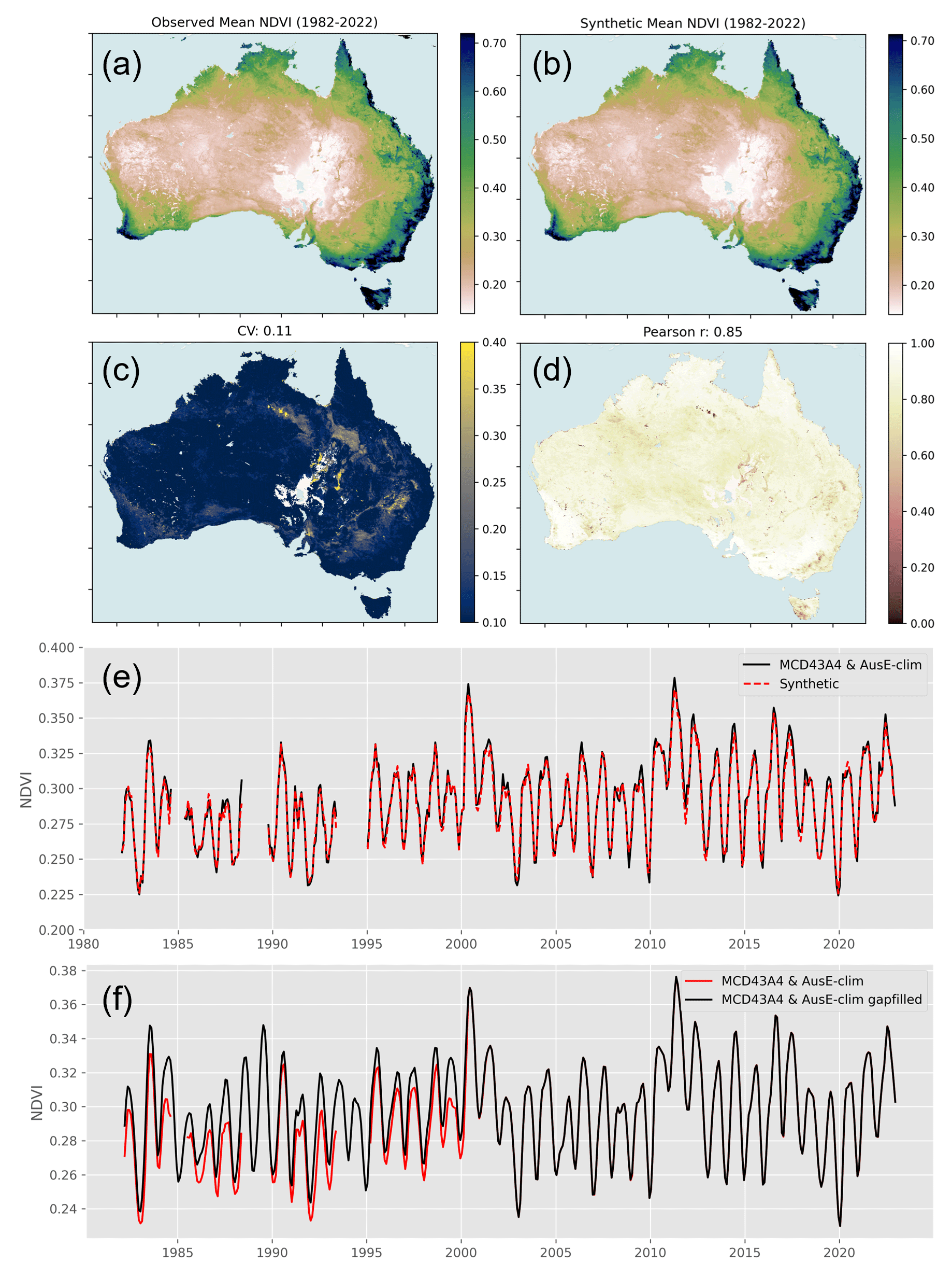
Figure 8 Evaluation of the synthetic NDVI built to gap-fill the NDVI_AusE-clim record. Panels (a) and (b) show the observed and synthetic long-term mean NDVI, respectively. (c) The per-pixel coefficient of variation (CV) between the observed NDVI and synthetic NDVI. (d) Same as (c) but for the Pearson correlation. (e) The continentally averaged observed and synthetic NDVI time series, where data gaps have been matched. (f) The results of gap-filling the merged NDVI_AusE-clim and NDVI_MCD43A4 time series.

3.3 Gap filling with the synthetic NDVI

The NDVI_SYN dataset record agrees exceptionally well with the joined NDVI_AusE-clim and NDVI_MCD43A4 series when aggregated across Australia (Fig. 8e). The time series of Fig. 8e is further disaggregated into high- and low-WCF regions (as per Fig. 2a) in Fig. A7, which reveals that in densely wooded regions, the synthetic NDVI tends to underestimate peak seasonal growth but otherwise captures seasonal timings and interannual variability (Fig. A7b). In the low-WCF regions (Fig. A7a), the synthetic NDVI closely matches with observations. At the pixel level, the long-term mean NDVIs of both datasets are virtually identical (Fig. 8a, b). Per-pixel Pearson correlation averages 0.85 across the continent (Fig. 8d). Areas of poorer correlation occur in western Tasmania and the highland forests of southeastern Australia – all areas that experience seasonal snowfall – and in regions with either anthropogenic water application (irrigation) or ephemeral, delayed water inundation (inland rivers in the arid interior). The mean relative error was also low, averaging 11 %, but with hotspots of greater error again occurring in the regions where water inundation is not dependent on direct rainfall (Fig. 8c). The results obtained before and after gap-filling NDVI_AusE-clim are presented in Fig. 8f. As the missing data tend to occur in the higher-NDVI regions (wetter, cloudier, and forested regions), gap filling has the tendency to increase the NDVI when averaged over the continent.

We present validation scatter plots and feature importance plots for the desert and non-desert GBM models in Appendix A (Fig. A8). In the non-desert region, 3-month cumulative rainfall and VPD are the key climate drivers of predictions, while in the desert region, 6-month cumulative rainfall, VPD, and incoming solar radiation are the key climate drivers.

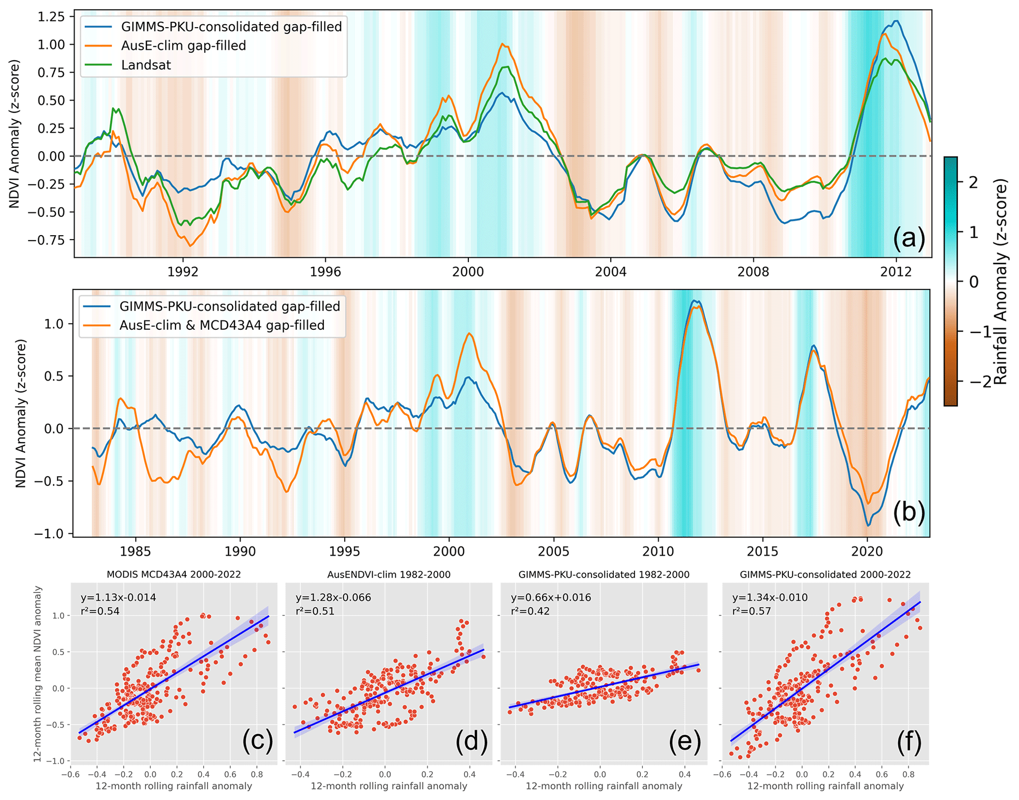
Figure 9 (a) Twelve-month rolling-mean standardised NDVI anomalies in the gap-filled NDVI_AusE-clim plotted alongside Landsat anomalies and NDVI_{PKU-consolidated} anomalies. Gaps in the NDVI_{PKU-consolidated} dataset have been filled using the same synthetic data and procedure as for NDVI_AusE-clim. All datasets are matched to Landsat data gaps. (b) Twelve-month rolling-mean standardised anomalies in the NDVI_{PKU-consolidated} (gap-filled in the same manner as in a) and NDVI_AusE-clim joined with NDVI_MCD43A4 (1982–2022 climatology). (c–f) Relationships between 12-month standardised rainfall and NDVI anomalies averaged across Australia for different periods and different products. Rainfall and NDVI_AusE-clim and NDVI_{PKU-consolidated} anomalies have been calculated against a 1982–2022 baseline. NDVI_MCD43A4 anomalies have been calculated against a 2000–2022 baseline. The slope coefficient can be considered an approximation of the sensitivity of NDVI to anomalous water supply aggregated over the continent. Note that the slope and intercepts for GIMMS-PKU-consolidated are slightly different to those in Fig. 3 owing to gap filling.

3.4 Assessing interannual variability

Comparing the calibrated, harmonised, and gap-filled NDVI_AusE-clim dataset with rolling annual-mean NDVI_Landsat anomalies in Fig. 9a reveals a good level of agreement in both the timing and magnitude of interannual variability (IAV) throughout the 1988–2012 period. NDVI_{PKU-consolidated} is also shown for comparison, and gaps in the NDVI_{PKU-consolidated} dataset have been filled using the same synthetic data and procedure as for NDVI_AusE-clim to facilitate a more straightforward comparison and continuous time series. NDVI_AusE-clim consistently outperforms NDVI_{PKU-consolidated} throughout the Landsat series. The IAV in NDVI_AusE-clim is further assessed in Fig. 9b, where the full time series (1982–2022 when NDVI_AusE-clim is joined with NDVI_MCD43A4) and NDVI_{PKU-consolidated} are plotted together as rolling annual-mean standardised anomalies against the same 1982–2022 climatology. NDVI_AusE-clim clearly displays greater IAV in the pre-MODIS era. We repeat the same analysis as in Fig. 3d–f but this time include NDVI_AusE-clim. The NDVI–rainfall relationships show that NDVI_AusE-clim reports a similar water-supply sensitivity and correlation in the 1982–2000 period (slope = 1.28, r²=0.51; Fig. 8d) to those reported by MODIS for the 2000–2022 period (slope = 1.13, r²=0.54; Fig. 9c). Again, while we may expect some changes in water-supply sensitivity over the decades due to effects such as CO₂ fertilisation, water supply sensitivity ought to remain relatively stationary, and we take the correspondence between NDVI_MCD43A4 sensitivity and NDVI_AusE-clim sensitivity as an indication that NDVI_AusE-clim is responding realistically to interannual variations in rainfall.

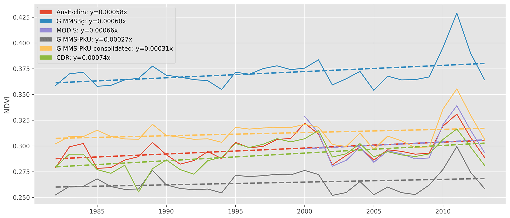
Figure 10 Annual average NDVI trends summarised over Australia for the overlapping period of 1982–2013. All data gaps have been matched between datasets, and the datasets have been reprojected to match the resolution of GIMMS3g. Note that AusENDVI-clim and noclim have both had data gaps filled to facilitate better annual averaging (i.e. so that all years have values). Trend lines have been fitted using ordinary least-squares regression, and coefficients are expressed in terms of NDVI per year.

3.5 Annual-average trends

We also evaluated the annual-average NDVI trends across Australia to assess the performance of AusENDVI in reproducing greening trends observed in other products. Trends were calculated over the overlapping period of 1982–2013 using ordinary least-squares regression after aggregating NDVI data to annual means. AusENDVI closely reproduces the observable trends in NDVI_GIMMS3g (coefficients: AusENDVI-clim = 0.00056 NDVI yr⁻¹, AusENDVI-noclim = 0.00049 NDVI yr⁻¹, GIMMS3g = 0.00062 NDVI yr⁻¹; Fig. 10). Trends in NDVI_MCD43A4 over the shorter interval from 2000–2013 displayed a similar slope to AusENDVI and GIMMS3g (0.00051 NDVI yr⁻¹). Trends in the two GIMMS-PKU products are approximately half those of the other products.

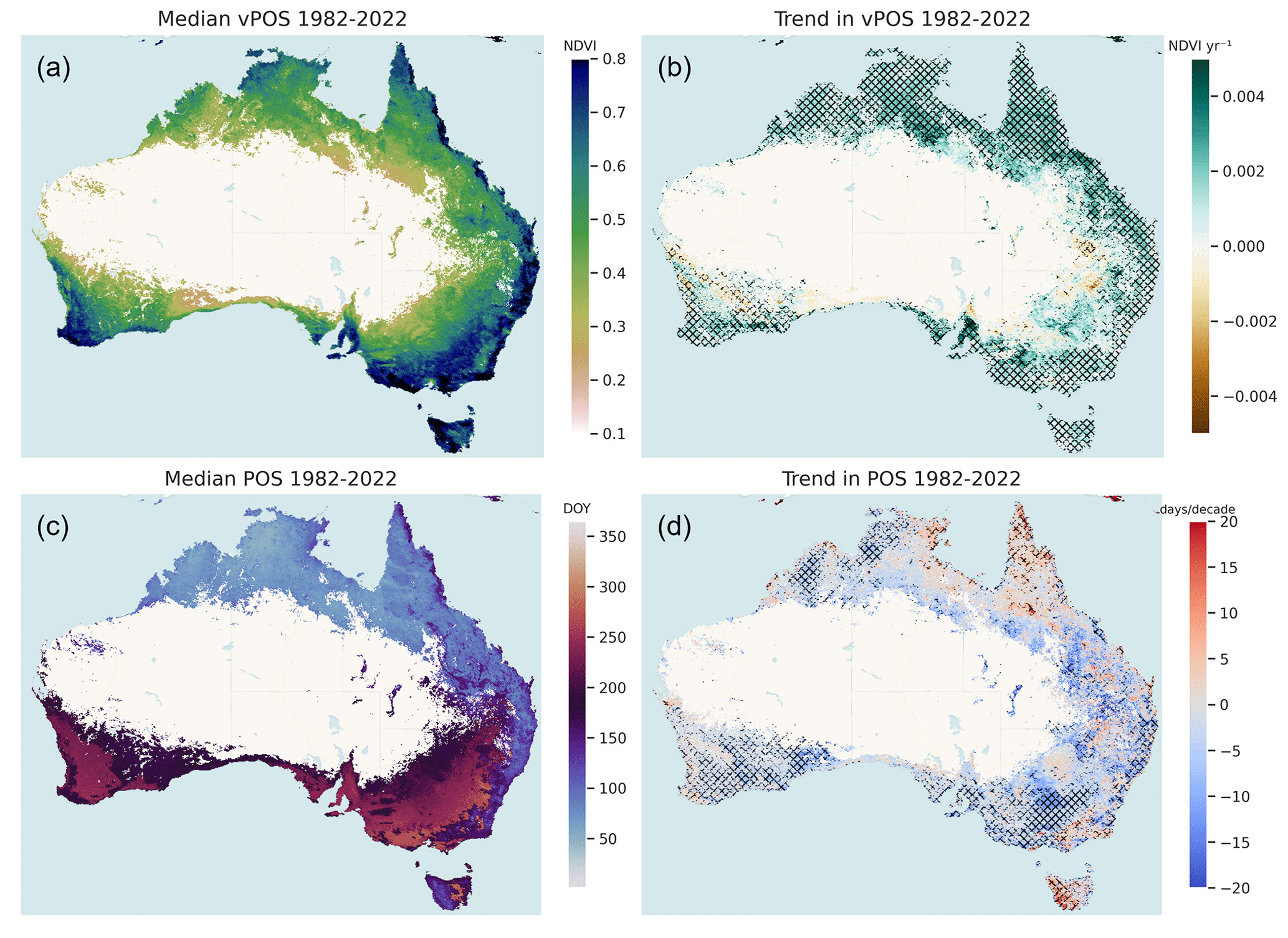
Figure 11 (a) The median annual peak NDVI value (vPOS) from 1982–2022. (b) Theil–Sen robust-regression trends in vPOS. (c) Median day of year that peak NDVI occurs (POS), 1982–2022. (d) Theil–Sen robust-regression trends in POS. Hatching on the trend plots indicates significance at α = 0.05 according to a Mann–Kendall test. All plots are derived from the gap-filled clim NDVI_AusE dataset. Non-seasonal areas have been masked using the method described in Sect. 2.4.

3.6 Trends in peak-of-season phenology

Per-pixel trends in vPOS and POS and the 40-year median values for these statistics are shown in Fig. 11. Trends in vPOS are almost universally positive across the continent (hatching indicates a significant trend) with the exceptions of the inland northern Murray–Darling Basin, the eastern periphery of the Wheatbelt in Western Australia (WA), and the region north of Adelaide (Fig. 11b). The positive trends observed in the major agricultural region of the Murray–Darling Basin and the northern half of the Western Australian Wheatbelt are non-significant. The distributions of trends in vPOS, stratified by bioclimatic region, reveal that the highest median trends are recorded in the tropics and savanna regions, at 0.0013 and 0.0014 NDVI yr⁻¹, respectively (Fig. A9a–e). The Mediterranean region has the lowest median trend at 0.0009 NDVI yr⁻¹.

Trends in the day of year that peak NDVI occurs (POS) are negative across much of the continent, suggesting that there is a general tendency for NDVI to peak earlier in the year across Australia. Significant negative trends occur in the agricultural zones of the Mediterranean bioclimatic region, the Great Western Woodlands that border the eastern margin of the Western Australian Wheatbelt, the western half of the Nullarbor Plain, parts of the Riverina agricultural region of southwestern New South Wales and extending into Victoria, and western parts of the northern tropical savanna. These significant negative trends are reflected in the POS trend distributions in Fig. A9f–j, where the median trends in the warm temperate and Mediterranean regions are highest at 3.4 and 2.3 days per decade, respectively. Significant positive trends (the peak NDVI occurring later in the year) are observed in tropical northern Queensland and western Tasmania and can be as high as 5–10 days per decade.

4 Discussion

4.1 Limitations of existing global products and improvements shown by AusENDVI

We expected to identify differences between NDVI_AVHRR and NDVI_MCD43A4 given the differences in spectral sampling between sensors and their different pre-processing and atmospheric-correction methods, spatial resolutions, and temporal-compositing techniques. Likewise, comparatively low correlations in the densely vegetated regions were also expected due to the total variance in evergreen forests being smaller than that for seasonal vegetation (grassland and croplands), and therefore, assuming a similar level of unexplained variance (noise), correlations should necessarily be weaker. Nonetheless, we were surprised by the fairly large inconsistencies between NDVI_GIMMS3g, NDVI_CDR, and NDVI_GIMMS-PKU in representing the seasonal dynamics of Australia's densely vegetated regions (e.g. Fig. 3k). Why this is the case deserves a greater focus of study than we devote here but is likely related to some combination of the presence/absence of BRDF and water-vapour corrections, varying contamination by clouds, and any gap-filling procedures applied. Regardless of the reasons why, the intercomparison between NDVI_AVHRR products highlights that global datasets, while often performing adequately when statistics are aggregated at the global or continental scale, can mask disparities that are important at the regional to local scale (Meyer and Pebesma, 2022). We advocate closely examining regional and local contexts to assess how suitable a given NDVI dataset is for a particular use case. For example, in Australia, seasonal cycles in NDVI_CDR are highly suspect and thus should not be relied upon for phenology studies. However, NDVI_CDR has a comparatively low relative error when compared with NDVI_MCD43A4 and displays reasonable interannual variability, so it would likely be more suited to long-term studies of agricultural drought frequency or the impacts of CO₂ fertilisation on canopy cover (assuming that sensor transitions are filtered). In Australia, the best use of NDVI_{PKU-consolidated} is likely the reverse: its representation of seasonal cycles agrees well with NDVI_MCD43A4, while IAV is subdued in the pre-MODIS era, which could lead to incorrect conclusions regarding shifting sensitivities to water supply in Australia's water-limited ecosystems. In general, we urge caution in using existing global NDVI_AVHRR products for studying vegetation trends and seasonality in Australia. AusENDVI shows significant improvement over existing global datasets in this respect. The improved correspondence in seasonal cycles between AusENDVI and NDVI_MCD43A4 provides evidence that AusENDVI is more suitable for exploring longer-term changes to Australia's vegetation phenology. Moreover, the addition of climate features to the calibration and harmonisation also appears to have improved the representation of long-term interannual variability and trends in annual average NDVI; thus, AusENDVI-clim should likewise offer a better basis for studying the shifting frequency of extreme climate events and their impact on the terrestrial biosphere.

4.2 Synthetic NDVI

The creation of a synthetic NDVI using only climate, CO₂ concentration, and woody-cover fraction as predictors revealed a high degree of predictability in NDVI over much of Australia. Regions of lower predictability were located where the water supply is, either from elsewhere or delayed (ephemeral inland rivers) or from irrigation. In the absence of features that could describe the water supply without rainfall, NDVI patterns in these zones will continue to be difficult to estimate if direct satellite observations are unavailable. Notwithstanding some spatial variability in per-pixel predictability, in general, the high degree of agreement between observed and synthetic NDVI presents the prospect of extending the synthetic NDVI further back in time through the observational climate record, which in Australia is reliable throughout much of the 20th century. In land surface models (LMSs), a dynamic phenology algorithm is an important sub-model which influences the overall carbon cycle, evapotranspiration, and energy balance of the model (Chen, 2022). The long-term record of synthetic NDVI developed here could, therefore, prove useful for validating the development of process-based phenology models for Australia's diverse range of vegetation and climate. Or, with empirically validated NDVI–LAI (leaf area index) relationships, AusENDVI could be used as a phenology forcing during the pre-satellite era for the many LSMs that do not dynamically simulate LAI.

4.3 Sources of uncertainty and future work

There are several sources of uncertainty in AusENDVI. Firstly, the climate and landscape features used are subject to their own uncertainties, which will undoubtedly propagate into both the calibration and harmonisation as well as the gap filling with synthetic NDVI. For example, rainfall station observations in the arid interior of Australia are relatively sparse, so errors in the spatial interpolation of rainfall are highly likely. Uncertainties in the NDVI_CDR product are also likely to be transmitted to our dataset. Future work may include a greater treatment of uncertainty through ensemble modelling, where climate features (e.g. different rainfall and solar-radiation datasets) and model types used for fitting are iterated to generate an uncertainty envelope. We also aim to assess how well the NDVI from the Visible Infrared Imaging Radiometer Suite (VIIRS) agrees with NDVI_AusE and NDVI_MCD43A4 over Australia. Should there be a substantial discrepancy, the methods described here could be applied to VIIRS to create an ongoing, updated NDVI dataset for Australia that can continue to form the foundation for continental-scale studies of terrestrial ecosystem change. Irrespective, we argue that our AusENDVI estimates are based on the best available data, while the gradient-boosting models have gone through extensive cross-validation. Therefore, we contend that the resulting trends should be more accurate than any alternative NDVI dataset.

4.4 Trends in peak-of-season phenology

We identified advances in the timing of POS across much of Australia's land mass (though not all). Over the Mediterranean, warm temperate, and cool temperate bioclimatic regions, the median peak phenology trends were −2 to −3 days per decade. Advances in plant maturity in the Southern Hemisphere from field data are also reported by Chambers et al. (2013), who find that the mean rate of change in plant maturity is 14 days per decade, mostly from temperate regions (63 % of their data are from grapevines). This rate of change is comparable to the per-pixel rates of change in POS that are seen in parts of the Mediterranean and warm temperate regions, where it is not uncommon to see negative trends ranging from 10–15 days per decade (Fig. 11d). However, the magnitude of a trend is influenced by the length of the time series, so comparisons with variable-length field data are difficult, and shorter records are more likely to report a larger rate (Chambers et al., 2013). Advances in the timing of POS could be due to a combination of climate drivers. In the Northern Hemisphere, warming has led to earlier peak greening (Huang et al., 2023; Liu et al., 2021; Park et al., 2019). Warming can accelerate metabolism, so where water is non-limiting, leaf development can be faster. However, temperature increases also increase vapour pressure deficits, which decrease water-use efficiency and can reduce plant productivity, though this effect may be compensated for by enhanced CO₂ (Rifai et al., 2022; Dusenge et al., 2019). Changes in the timing of peak rainfall may also contribute to shifts in the timing of peak NDVI. The timing of peak climatological rainfall has shifted since 1960 (Fig. A10a–c), and there is some coincidence between trends in POS and shifts in rainfall POS (e.g. an advancement around Adelaide). The goal of this study is not to draw conclusions on the likely drivers of seasonality change in Australia but to argue that our dataset provides a more reliable means for tackling these questions. Future work will delve into a greater suite of phenology metrics (e.g. start of season, end of season, and growing-season length; Xie et al., 2023) and explore the drivers of phenological change.

The pervasive positive trends in vPOS are consistent with results elsewhere and are likely due to the impacts of CO₂ fertilisation, which allows a given amount of precipitation to sustain a greater maximum level of plant production over time (Donohue et al., 2009, 2013; Rifai et al., 2022; Ukkola et al., 2016). Increases in the magnitude of austral spring and summer rainfall in northern Australia are also likely to have contributed to the widespread increase in vPOS in tropical Australia (Fig. A10d). It is also likely that improving agricultural practices has increased the maximum NDVI in the rain-fed cropping regions, especially in South Australia and Victoria, where positive vPOS trends are significant. Trends in maximum NDVI in the Western Australian Wheatbelt are also positive but contrast with the fact that WA has seen a widespread autumn drying trend (Fig. A10d). We speculate that agricultural innovation there has counteracted a drying trend that would otherwise have reduced foliage cover.

5 Data availability

AusENDVI is openly available at https://doi.org/10.5281/zenodo.10802703 (Burton et al., 2024) and consists of several datasets. Each dataset has a description in the attributes of the NetCDF file that defines its provenance. A short description of each dataset is provided below as an additional reference. All datasets are in EPSG:4326 projection, have a spatial resolution of 0.05°, and have monthly temporal resolution. A Jupyter notebook demonstrating how to load, plot, mask, reproject, and gap-fill AusENDVI datasets is also provided at the above link.

AusENDVI-clim_gapfilled_1982_2013. Calibrated and harmonised NOAA Climate Data Record AVHRR NDVI data from January 1982 to December 2013. This version of the dataset used climate data in the calibration and harmonisation process. The dataset has been gap-filled using the methods described in Sect. 2.3.

AusENDVI-noclim_1982_2013. Calibrated and harmonised NOAA Climate Data Record AVHRR NDVI data from January 1982 to December 2013. This version of the dataset did not use climate data in the calibration and harmonisation process, and the dataset has not been gap-filled.

AusENDVI-synthetic_1982_2022. This dataset consists of synthetic NDVI data that were built by training a model on the joined AusENDVI-clim and MODIS-MCD43A4 NDVI time series using climate, woody-cover fraction, and atmospheric CO₂ as predictors. AusENDVI-synthetic is used for gap filling.

AusENDVI-clim_gapfilled_MCD43A4_1982_2022. This dataset consists of calibrated and harmonised NOAA Climate Data Record AVHRR NDVI data from January 1982 to February 2000 joined with MODIS-MCD43A4 NDVI data from March 2000 to December 2022. This version of the dataset used climate data in the calibration and harmonisation process. The dataset has been gap-filled using the methods described in Sect. 2.3.

6 Code availability

The code to conduct all analysis described here is available in the open-source repository at https://doi.org/10.5281/zenodo.13831836 (Burton, 2024).

7 Conclusion

We calibrated and harmonised NDVI_CDR to NDVI_MCD43A4 for Australia using a well cross-validated gradient-boosting ensemble decision tree method. We developed two versions of the datasets: one that utilises climate data in the feature set to achieve the best possible agreement between NDVI_CDR and NDVI_MCD43A4 (AusENDVI-clim) and a second dataset that does not rely on climate data (AusENDVI-noclim). The resulting datasets have a spatial resolution of 0.05° and extend from 1982–2013 with a monthly time step. The better agreement between AusENDVI and MODIS in terms of IAV, seasonal variability, and long-term mean NDVI allows us to provide a complete 41-year dataset where the gap-filled AusENDVI-clim from January 1982 to February 2000 is joined with NDVI_MCD43A4 from March 2000 to December 2022. The advantages of AusENDVI are that (1) it closely reproduces the NDVI_MCD43A4 record in terms of seasonality, interannual variability, and trends in annual-average NDVI; (2) it reproduces annual anomalies in the Landsat NDVI record in the pre-MODIS era (back to 1988) and shows realistic rainfall-driven interannual variability back to 1982; (3) we developed a reliable method for gap-filling the AusENDVI record by creating a synthetic NDVI dataset using only climate, CO₂ concentration, and woody-cover fraction as predictors. The resulting dataset showed excellent agreement with NDVI_MCD43A4 and the recalibrated NDVI_AVHRR time series, providing confidence in its use for gap filling; (4) AusENDVI has a higher spatial resolution than any of the GIMMS-based datasets and is built using inputs that apply the full suite of atmospheric and BRDF corrections; and (5) the methods and code used for its development are entirely open source. No other existing product can lay claim to all these attributes, which is why we argue that AusENDVI is an important addition to the suite of NDVI products available. We contend that it is highly suitable for studying the impact of global environmental change on Australia's terrestrial vegetation.

Appendix A

Table A1 The hyperparameter grids used during the optimisation of the harmonisation model and the synthetic NDVI model. During model fitting, a random grid search was conducted with 250 iterations to identify the highest-performing set of hyperparameters.

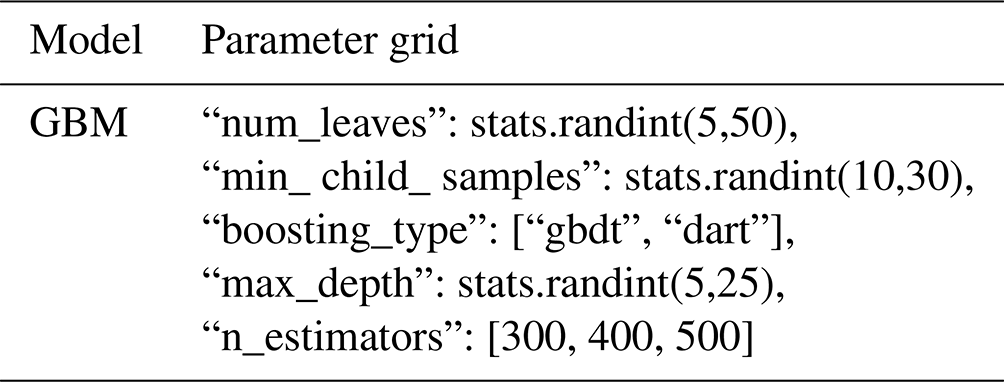
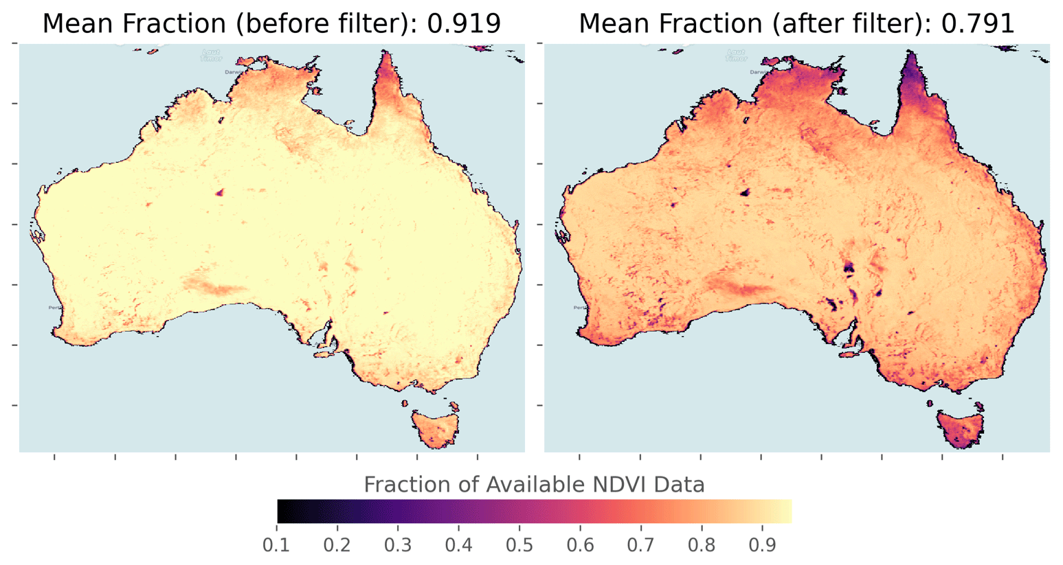
Figure A1 Available fractions of data before and after the additional filtering of NDVI_CDR data. A value of 1 means that all monthly time steps between 1982–2013 are preserved.

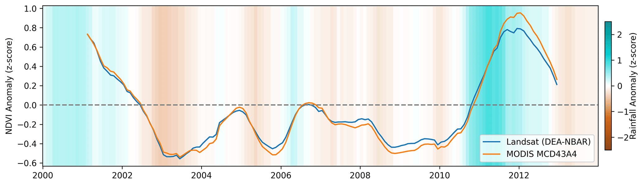
Figure A2 Standardised anomalies of the overlapping period between the MODIS MCD43A4 NDVI and the DEA's Landsat NDVI derived from the common baseline period of 2000–2012. Rainfall anomalies are derived from a longer baseline of 1982–2022.

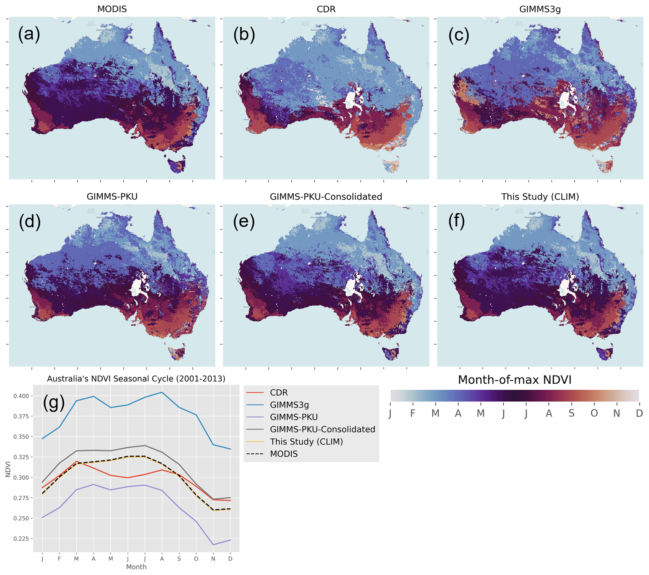
Figure A3 (a–f) Month that the maximum NDVI occurs, averaged from 2001–2013, for all NDVI datasets included in the intercomparison between NDVI products along with the AusENDVI-clim dataset of this study. (g) The climatological mean seasonal cycle of NDVI summarised over Australia.

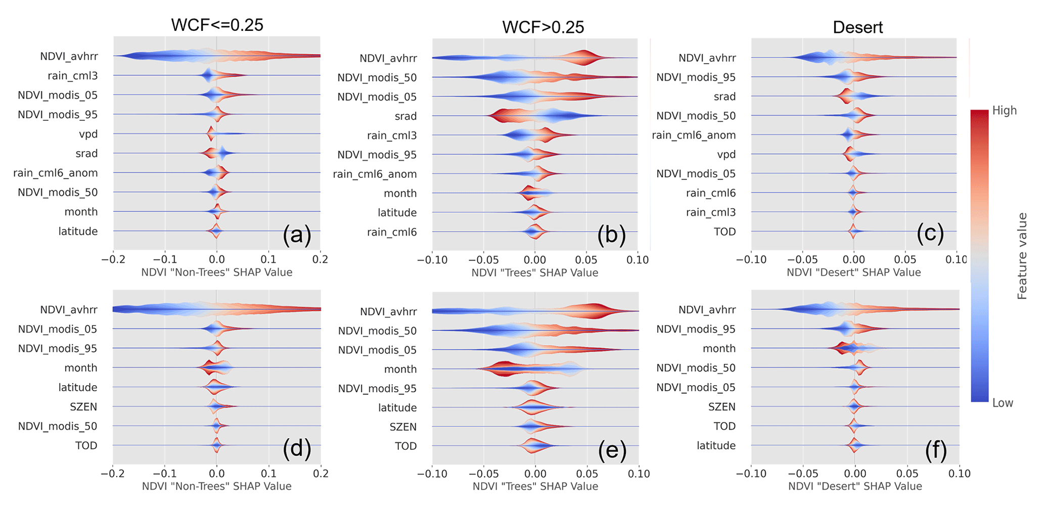
Figure A4 Feature importance plots for the calibration and harmonisation between NDVI_CDR and NDVI_MCD43A4. Panels (a)–(c) show the results for the clim model. Panels (d)–(f) show the same but for the noclim model type.

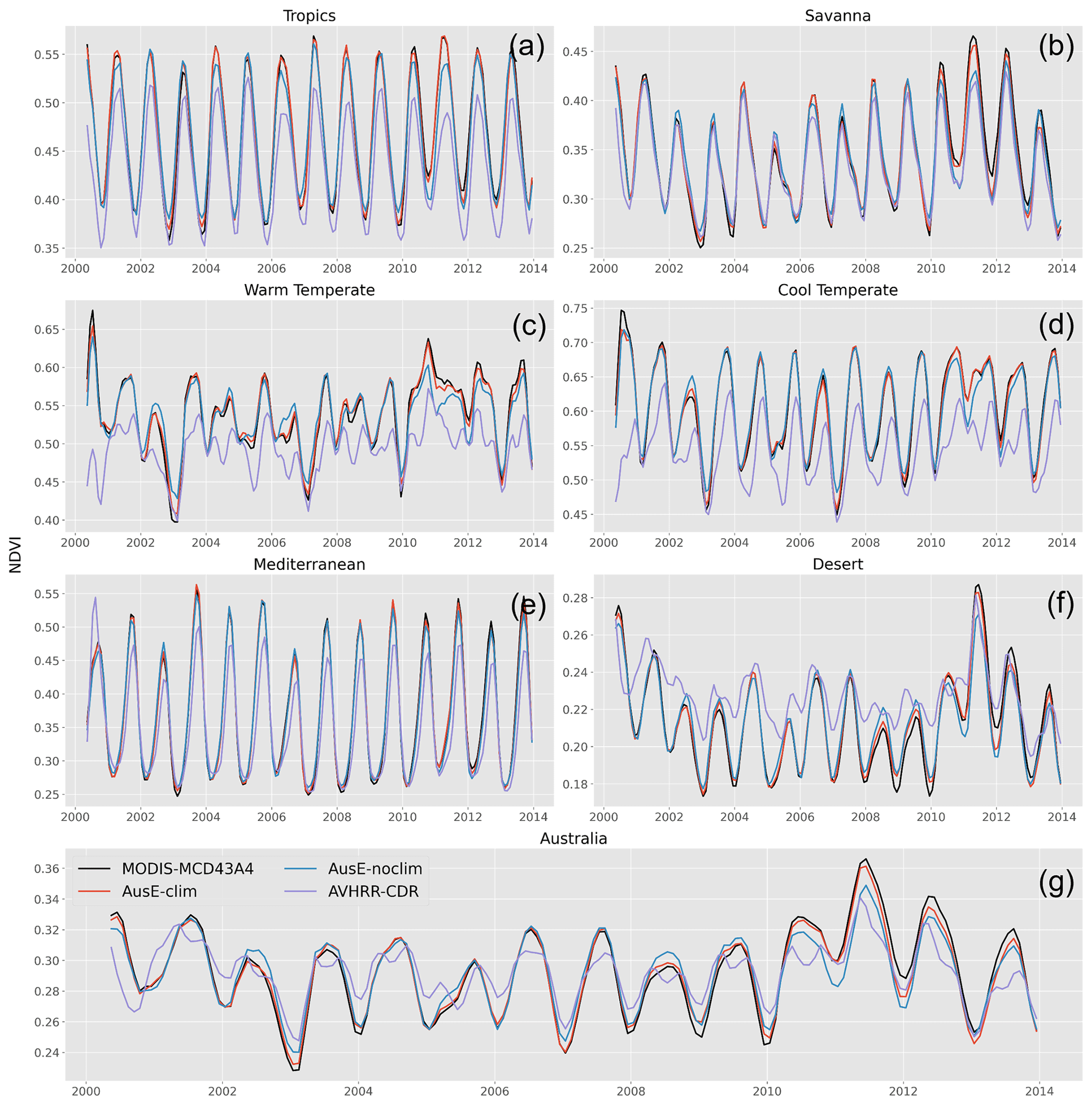
Figure A5 Per-bioregion (a–f) and Australia-wide (g) NDVI time series before and after the calibration and harmonisation of NDVI_CDR. The bioregions are defined in Fig. 2b. The time series have been smoothed with a 3-month rolling mean.

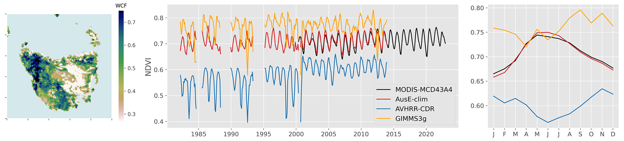
Figure A6 Same as Fig. 6d–f but including NDVI_GIMMS3g to demonstrate that the very strong increasing trend in NDVI_CDR is likely an artefact of sensor transitions and poor calibration.

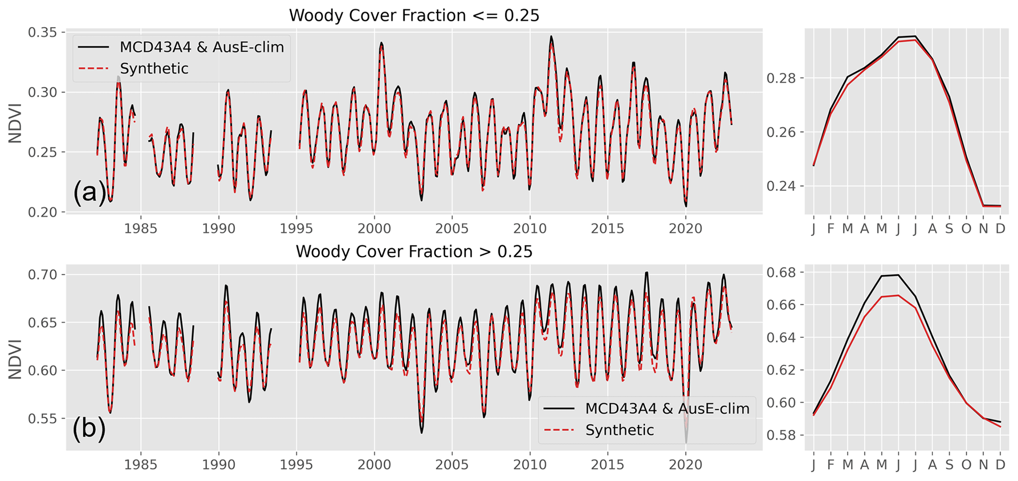
Figure A7 Evaluation of the synthetic NDVI built to gap-fill NDVI_AusE-clim disaggregated into high- and low-WCF regions. (a) Spatially averaged observed and synthetic NDVI time series over all continental areas where WCF is less than or equal to 0.25. (b) Same as (a) but for regions where WCF is greater than 0.25.

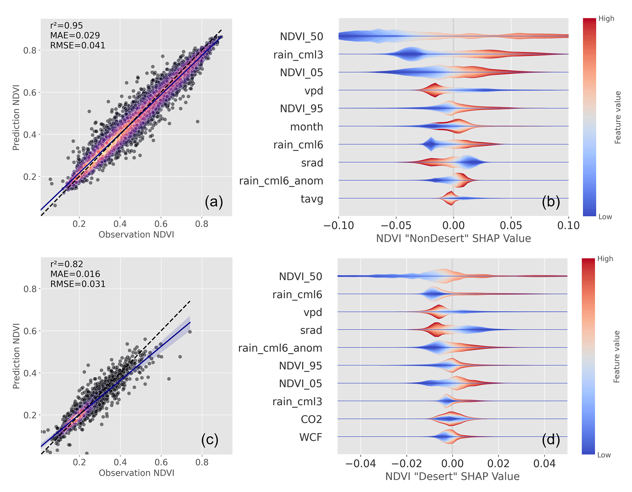
Figure A8 Validation scatter plots and feature importance plots for the gap-filling synthetic NDVI models. Panels (a) and (b) are for the non-desert model region, which covers the high- and low-woody-cover regions shown in Fig. 1a. Panels (c) and (d) are for the desert region.

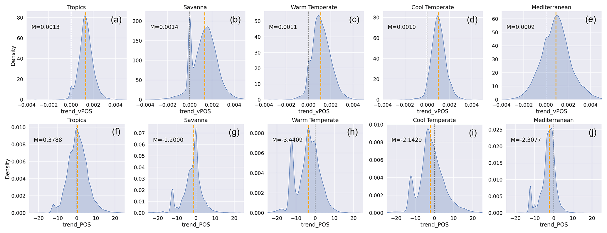
Figure A9 Distributions of pixel-level trends in vPOS (a–e) and POS (f–j) summarised by bioclimatic region (excluding the desert region as most of that region is masked as it is non-seasonal). “M” refers to the median slope value of the distribution and is indicated by the dashed orange line. The units for vPOS are NDVI yr⁻¹, and the units for POS are days per decade.

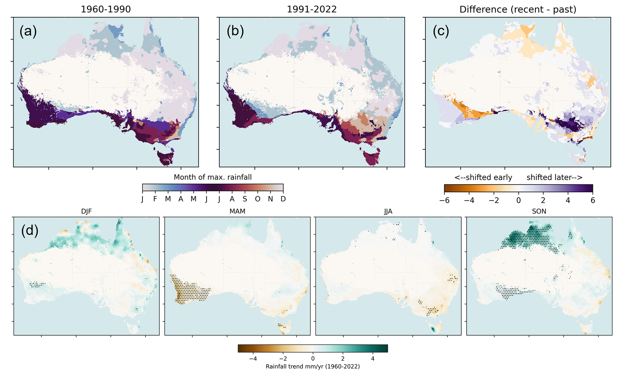
Figure A10 Changes to the timing and magnitude of rainfall in Australia. (a) The typical month that rainfall achieves its maximum value, averaged from 1960–1990. (b) Same as (a) but for a 1991–2022 climatology. (c) The difference between (a) and (b) where the 1991–2022 climatology is subtracted from 1960–1990. Orange colours indicate earlier peak rainfall in the more recent climatology (in number of months). If peak rainfall shifts from January in 1960–1990 to December in 1991–2022, this is recorded as earlier by 1 month. Purple colours indicate that peak rainfall occurs later in 1991–2022 compared with 1960–1990. If peak rainfall shifts from December in 1960–1990 to January in 1991–2022, this is recorded as later by 1 month. (d) Theil–Sen trends in the total seasonal rainfall from 1960–2022. Hatching indicates significance at 95 % confidence using a Mann–Kendall test.