GERB Obs4MIPs: a dataset for evaluating diurnal and monthly variations in top-of-atmosphere radiative fluxes in climate models

A newly available radiative flux dataset specifically designed to enable the evaluation of the diurnal cycle in top-of-atmosphere (TOA) fluxes as captured by climate and Earth system models is presented. Observations over the period 2007–2012 made by the Geostationary Earth Radiation Budget (GERB) instrument are used to derive monthly hourly mean outgoing longwave radiation (OLR) and reflected shortwave (RSW) fluxes on a regular 1° latitude–longitude grid covering approximately 60° N–60° S and 60° E–60° W. The impact of missing data is evaluated in detail, and a data-filling solution is implemented using estimates of broadband fluxes from the Spinning Enhanced Visible and Infrared Imager flying on the same Meteosat platform, scaled to the GERB observations. This relatively simple approach is shown to deliver an approximate improvement by a factor of 10 in both the bias caused by missing data and the associated variability in the error. To demonstrate the utility of this V1.1 filled GERB Observations for Climate Model Intercomparison Projects (Obs4MIPs) dataset, comparisons are made to radiative fluxes from two climate configurations of the Hadley Centre's Global Environmental Model: HadGEM3-GC3.1 and HadGEM3-GC5.0. Focusing on marine stratocumulus and deep convective cloud regimes, diurnally resolved comparisons between the models and observations highlight discrepancies between the model configurations in terms of their ability to capture the diurnal amplitude and the phase in TOA fluxes, details that cannot be diagnosed by comparisons at lower temporal resolutions. For these cloud regimes the GC5.0 configuration shows improved fidelity to the observations relative to GC3.1, although notable differences remain. The V1.1 filled GERB Obs4MIPs monthly hourly TOA fluxes are available from the Centre for Environmental Data Analysis, with the OLR fluxes accessible at https://doi.org/10.5285/90148d9b1f1c40f1ac40152957e25467 (Bantges et al., 2023a) and the RSW fluxes accessible at https://doi.org/10.5285/57821b58804945deaf4cdde278563ec2 (Bantges et al., 2023b).

1 Introduction

The balance between Earth's incoming and outgoing radiant energy at the top of the atmosphere, known as Earth's radiation budget (ERB), is the primary driver of the climate system. This essential climate variable is hence a fundamental quantity for understanding Earth's climate and its variability. Satellite measurements of Earth's reflected shortwave (reflected solar) and emitted thermal infrared (outgoing longwave) components of the ERB with dedicated broadband instruments began in 1975 with the ERB instrument on Nimbus 6 (Smith et al., 1977). Global observations spanning many years have been obtained from low Earth orbit satellites with the Earth Radiation Budget Experiment (ERBE) (Barkstrom, 1984) and Clouds and the Earth's Radiant Energy System (CERES) instruments (Wielicki et al., 1996) and for the tropics with the Scanner for Radiation Budget (ScaRaB) instrument on Megha-Tropiques (Roca et al., 2015). However, the Geostationary Earth Radiation Budget (GERB) experiment (Harries et al., 2005) is the only ERB mission to fly in geostationary orbit and is thus the only mission to provide high-time-resolution broadband observations of the top-of-atmosphere (TOA) energy.

Four GERB instruments have been deployed sequentially on the four Meteosat Second Generation satellites (Meteosat-8, Meteosat-9, Meteosat-10, and Meteosat-11). Since May 2004 they have provided TOA outgoing longwave radiation (OLR) and reflected solar (RSW) flux products broadly covering the geographical region 60° E–60° W and 60° N–60° S at a 15 min temporal resolution. The frequency and longevity of the observations enable the diurnal cycle to be resolved and facilitate the study of fast climate processes, such as cloud and aerosol, by quantifying their changing effect on the radiation balance over a range of timescales from minutes to years. Although the GERB data are only available for the portion of the globe observable from the Meteosat geostationary orbit, they provide broadband observations throughout the diurnal cycle. In contrast, other temporally resolved radiation budget datasets, such as the CERES Synoptic (SYN) products, use narrowband geostationary imager data to provide temporal resolution. These supplement, and are scaled to, the much lower temporal-resolution broadband observations from the low Earth orbiting CERES instruments themselves. GERB data have been used in the development and evaluation of the CERES temporal interpolation used in the SYN products (Doelling et al., 2013, 2016). The instantaneous GERB products have also been used to study and characterise diurnal variability (e.g. Comer et al., 2007; Gristey et al., 2018), the effects of cloud and aerosol on the radiation budget (e.g. Futyan et al., 2005; Slingo et al., 2006; Brindley and Russell, 2009; Pearson et al., 2010; Ansell et al., 2014; Milton et al., 2008; Banks et al., 2014), and the representation of these processes in selected numerical weather prediction and climate models (e.g. Allan et al., 2007, 2011; Greuell et al., 2011; Haywood et al., 2011; Mackie et al., 2017).

While the instantaneous GERB data have been extensively exploited, they are not currently provided in a format that facilitates easy comparison with climate or Earth system model output. In particular, they suffer from irregular spatial sampling, have a temporal resolution that is higher than that at which model radiation outputs are typically retained, and have a non-standard data format. This paper describes the production of a new monthly hourly mean data product, derived from the instantaneous GERB data, to circumvent these issues. This GERB Observations for Climate Model Intercomparison Projects (Obs4MIPs) dataset consists of monthly hourly mean TOA OLR and RSW fluxes provided at a 1° longitude–latitude spatial resolution for the GERB observation region. It provides a record covering several years that resolves the diurnal variation in the TOA OLR and RSW and is compatible with climate model output such as that produced for the recent Coupled Model Intercomparison Project 6 (CMIP6) (Eyring et al., 2016). The data are provided in Climate and Forecast (CF) v1.7 compliant netCDF format meeting the Obs4MIPs submission requirements (Waliser et al., 2020). In the following sections we outline the methodology and provide a detailed analysis of the impact of missing data. We propose and evaluate a relatively simple approach to fill data gaps before providing an illustration of how the new dataset may be employed to assess climate model performance.

2 Production of the GERB Obs4MIPs monthly hourly average products

Two versions of the GERB Obs4MIPs monthly hourly average products have been released. The first version (GERB-HR-ED01-1-0) (Bantges et al., 2021a and b) is produced solely from the GERB data that are available, hereafter referred to as V1.0 or “unfilled” GERB Obs4MIPs products. The second, improved version (GERB-HR-ED01-1-1) (Bantges et al., 2023a and b), which is the primary focus of this paper, uses supplementary information derived from the narrowband Spinning Enhanced Visible and Infrared Imager (SEVIRI) flying on the same Meteosat Second Generation platform as GERB (Schmetz et al., 2002), scaled to GERB to fill missing hours of GERB data before calculating the monthly hourly average. These products are referred to hereafter as V1.1 or “filled” GERB Obs4MIPs products: we show how they are an improvement on the V1.0 release in both the amount of data available and the associated uncertainty.

2.1 Baseline methodology

The GERB Obs4MIPs OLR and RSW fluxes discussed here are based on the observational record from the GERB-1 instrument on Meteosat-9, which ran from May 2007 to January 2013. As noted above, the goal is to create monthly mean, diurnally resolved OLR and RSW fluxes at an hourly resolution on a regular 1° latitude–longitude grid.

The starting points for creating the averages are the GERB level-2 High Resolution (HR) flux products (Brindley and Russell, 2017), which are produced to facilitate averaging and re-gridding of the GERB instantaneous fluxes. The GERB HR fluxes are a temporally interpolated, resolution-enhanced version of the original GERB observations derived using spatial information on the scene variation within the GERB footprint from the SEVIRI instrument. GERB HR fluxes are presented on a regular viewing angle grid, which has a spatial resolution of 9 km at the sub-satellite point. They give a “snapshot” of the fluxes at a 15 min temporal resolution, aligned to the observation times of the SEVIRI instrument flying on the same satellite.

The GERB instrument operates with the use of a rotating mirror which effectively steps the linear detector array aligned approximately north–south with respect to Earth, east–west, and then west–east across Earth's disc. Early in the mission, the mirror briefly became stuck in a position which allowed direct solar illumination of a portion of the detector array, resulting in several pixels being lost. To circumvent the possibility of this reoccurring, subsequent operations were restricted such that diurnally resolved observations are not collected for around 5 weeks either side of the equinoxes. As a result, the production of unfilled GERB Obs4MIPs monthly hourly fluxes was initially restricted to the months of November, December, January, May, June, and July, avoiding the months impacted by these operating restrictions. As will be demonstrated in Sects. 2.3 and 3.2, implementing a relatively simple data-filling approach additionally allows the construction of February and August monthly hourly averages within tolerable uncertainties.

Figure 1 summarizes the steps used to produce an unfilled Obs4MIPs product from the GERB HR 15 min fluxes for both OLR and RSW. The initial step involves averaging the GERB HR data to an hourly 1° latitude–longitude scale. To achieve this, area-weighted averaging of all the available points whose centres fall within each 1° latitude–longitude grid box is performed across the region of 60° N–60° S and 60° E–60° W for points with a viewing zenith angle of less than 70°, which is the maximum viewing angle recommended in the GERB quality summary (Russell, 2017) for averaging to Earth grids. This is followed by straight averaging over all the available 15 min products for each UTC hour, centred on the half-hour. When there are no missing data, the hourly average of each 1° latitude–longitude grid box would, depending on the location, comprise between 6 and 169 GERB HR points at each of the four time slots obtained during the hour. However, an average is still formed if some time slots or contributing pixels are missing, as long as there is at least 1 GERB HR pixel within the 1° latitude–longitude grid box at one time slot in the hourly bin. For OLR, this process is performed directly on the fluxes. For RSW, the fluxes are converted to albedo before both spatial and temporal averaging and converted back to flux at the hourly 1° latitude–longitude scale, using the incoming solar flux representative of the centre of each 1° latitude–longitude grid box and hourly bin (i.e. at 00:30, 01:30 UTC, etc.). As the total solar irradiance and the Earth–Sun distance do not change during the conversion to albedo and back to flux, this becomes purely an adjustment in the solar zenith angle to the centre of the grid box and hourly bin. The process is equivalent to multiplying each flux by the ratio $\cos \left({\mathit{\theta }}_{\mathrm{local}}\right)/\cos \left({\mathit{\theta }}_{\mathrm{centre}}\right)$, where θ_local is the solar zenith angle at the HR pixel time and position and θ_centre is the solar zenith angle at the 1° latitude–longitude centre at half past the hour. This treatment mitigates any bias that might result from only some of the 15 min time slots within the hour being available and enables hourly fluxes to be derived in the presence of missing data. It also corrects for the variation in solar zenith angles that occurs due to the row-to-row time variation of the GERB HR, which is a consequence of these products being interpolated to match the 12 min SEVIRI scanning cycle. We note that the GERB HR RSW products use a fixed location-independent twilight model based on the model derived from CERES observations (Kato and Loeb, 2003) for solar zenith angles between 85 and 100°, and they set RSW to zero for solar zenith angles greater than 100°. For consistency, this treatment is also applied to the GERB Obs4MIPs products at the daily hourly 1° latitude–longitude scale using the solar zenith angle of the centre of the grid box and an hourly bin. Hence, these model twilight and nighttime RSW HR fluxes, which are not GERB observations, are not included in the spatial or temporal averaging to the daily hourly 1° latitude–longitude scale if the central solar zenith angle is less than 85°, but they are used to replace grid-box values when the central solar zenith angle is equal to or exceeds 85°. For both OLR and RSW, in the initial unfilled product version, the resulting 1° latitude–longitude hourly fluxes are then averaged over all available days of the month to give the final 1° latitude–longitude unfilled monthly hourly products.

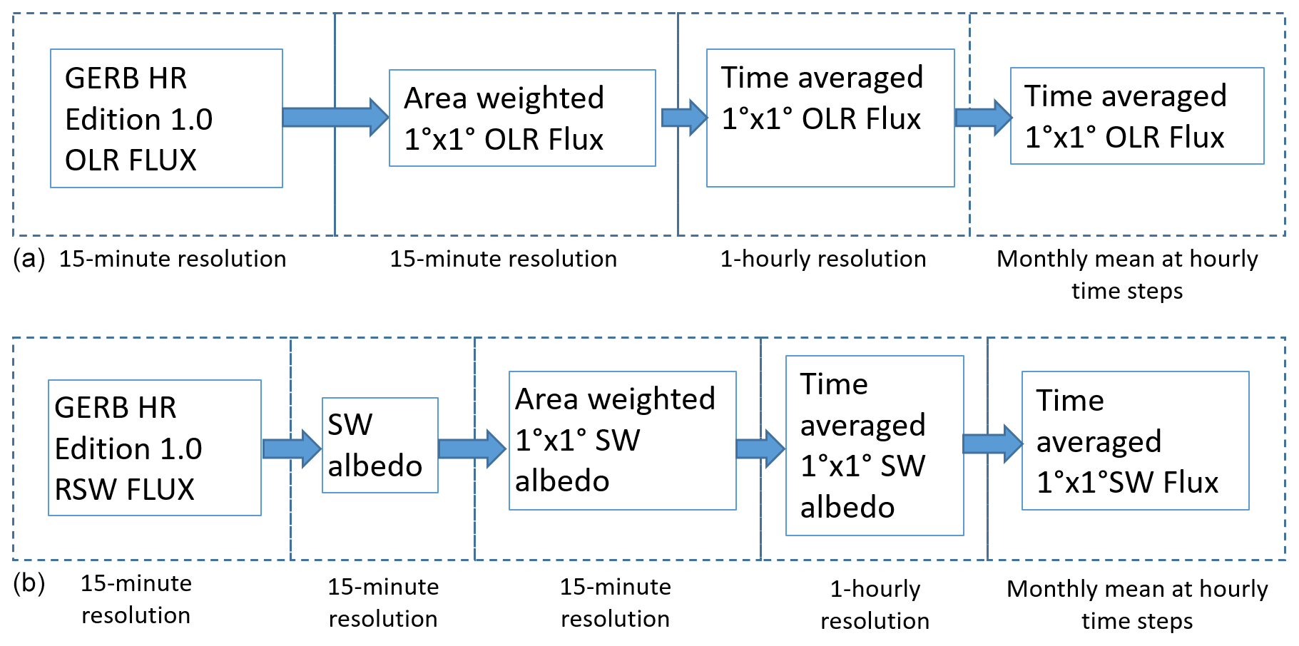
Figure 1 Schematic of the steps employed in the production of the OLR (a) and RSW (b) V1.0 unfilled monthly hourly average Obs4MIPs products from the GERB HR Edition 1 fluxes.

2.2 Missing GERB observations

Calibration operations and other planned and unplanned operational issues result in observational gaps over the whole of the GERB region for 1 h or more or, more occasionally, days at a time, and they manifest as missing time slots in the HR record. This leads to a significant number of cases where there are no observations available for a given hour on a particular day, which without further data processing appear as gaps at the daily hourly scale that result in errors in the Obs4MIPs monthly hourly averages. A summary of the number of missing days of hourly GERB data for the whole GERB-1 record is shown in Fig. 2 as a function of hour and month. Hours with complete data are shown in white, and those with more than 22 missing days are shaded grey. Hours where there are between 1 and 5 missing days in the month are shaded turquoise, and cases with between 5 and 22 missing days are shaded pale green. The boundaries of 5 and 22 missing days are highlighted as these limits correspond to the maximum number of missing days allowed in the data released for the unfilled and filled products, respectively (see Sect. 3). There is an uneven distribution of missing data through the record, with a few months (e.g. December 2012) showing almost complete data coverage and others showing varying degrees of incomplete coverage at all hours. As previously discussed, operating restrictions in the months around the equinoxes are responsible for an almost complete absence of observations during March, April, September, and October, resulting in these months being greyed out. These restrictions are also responsible for the pattern of missing data in February and August, where the latter parts of these months are always missing. Persistently higher amounts of missing data in the hours around midnight for November and May are a result of data excluded due to stray light contamination at the start of each of these months. The other cases with more than 5 missing days across all hours (e.g. May and December 2007 and 2008) are at least in part associated with extended instrument outages and in some cases satellite outages, leading to the loss of multiple days of data. Apart from these cases, missing data are generally randomly distributed through the month, and the specific days that are missing generally change from hour to hour. Hence, the effect of missing data on the monthly hourly averages may also affect the fidelity of the diurnal cycle in unexpected ways.

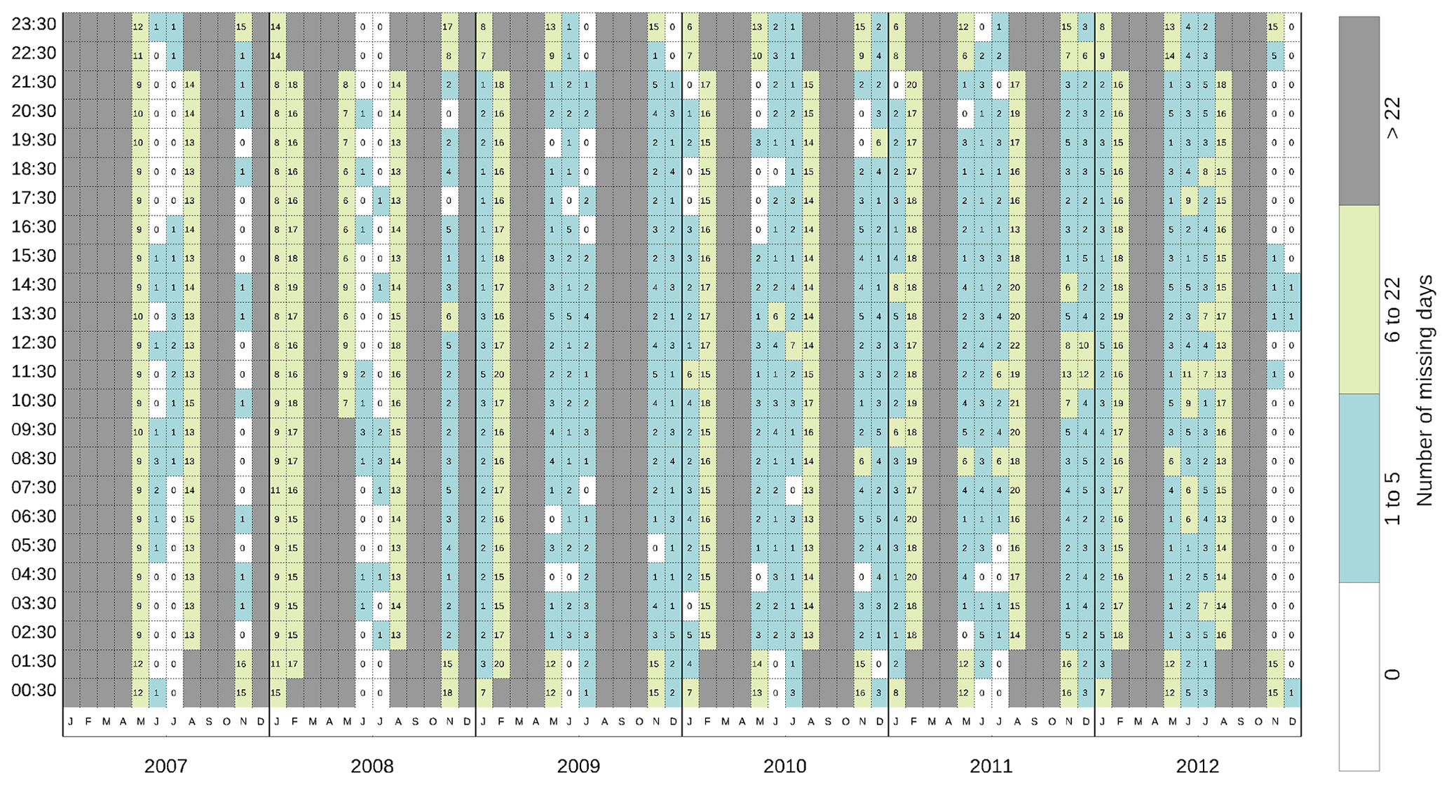
Figure 2 Number of missing days of data per month as a function of the hour and year. Cells are coloured according to the number of missing days for that hour and month, with turquoise indicating 5 or fewer missing days, pale green between 6 and 22 missing days, and grey more than 22 missing days. Where there are 22 or fewer missing days, the actual number of days missing is indicated in the box. The colour divisions are chosen to highlight the hours with no missing days and to delineate the data included in the unfilled and filled products as discussed in Sect. 3.

2.3 Strategy for filling missing GERB data

Considering the amount of missing data in the GERB dataset and the effect this is likely to have on the monthly hourly average, it is clearly desirable to investigate methods for filling in some of the missing information. Given the pattern of missing data, with multiple occurrences of several hours and indeed several days missing in some cases, filling the gaps by interpolating the existing GERB observations is not viable. Ideally, an alternative source of information responsive to the meteorology present during the periods of missing data that can be used to fill the gaps in the record is required.

The prime instrument on the Meteosat Second Generation satellites is SEVIRI. This instrument provides radiances in 11 narrowband channels from 0.635 to 13.4 µm every 15 min with a resolution of 3 km at the sub-satellite point. The GERB HR products, on which the Obs4MIPs dataset is based, are provided as a snapshot at the time of the corresponding SEVIRI observation, at a resolution of 3 × 3 SEVIRI pixels and on a grid aligned with the SEVIRI grid. As part of the GERB processing, an empirical narrowband-to-broadband conversion is applied to the SEVIRI radiances to derive estimates of the broadband radiances (Clerbaux et al., 2008a, b). These so-called “GERB-like” radiances are converted to fluxes with the same conversion factor used to determine the GERB fluxes from the GERB radiances (Dewitte et al., 2008).

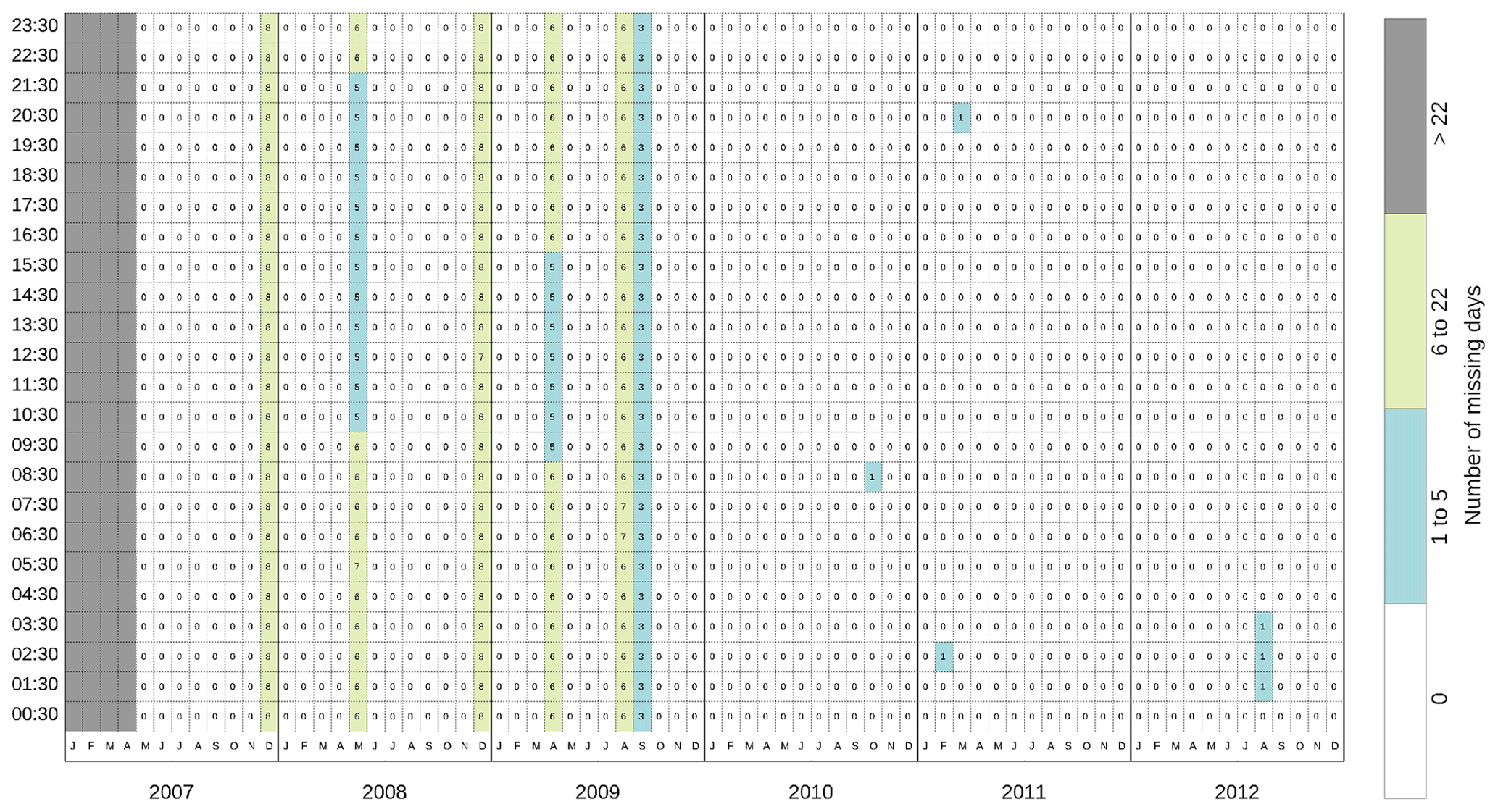
The SEVIRI-based GERB-like fluxes suffer from significantly fewer missing data than the original GERB record (compare Figs. 3 and 2). Except for a few extended outages in the first few years which are a result of satellite level anomalies, nearly all the data missing in the GERB record are present in the GERB-like record. Thus, the latter record may be useful for filling much of the missing GERB data.

Figure 3 As in Fig. 2 but for GERB-like observations.

The way in which the GERB-like fluxes are used in the GERB processing places no requirements on their absolute accuracy and limited requirements on their relative accuracy. Our expectation is that differences between GERB and GERB-like fluxes due to deficiencies in the narrowband-to-broadband conversion and due to the calibration of the original narrowband observations will need to be addressed before the GERB-like data can be used to replace missing GERB data. Narrowband-to-broadband conversion errors will likely have scene and angular dependencies that do not vary a great deal over time, except in relation to these variables. Conversely, calibration-related errors would be expected, at first order, to manifest across different scenes in a similar, reproducible way, but they may vary in time. There may also be cross terms where calibration changes manifest across the scenes differently due to variation in the weighting of the channels between scenes. For the GERB-like data to be a suitable proxy for the GERB data, we need to understand, correct, and account for not just the average offset between GERB and GERB-like but also the way in which the difference varies with scene, time of day, and location.

Figures 4 and 5 show the spatially resolved monthly hourly mean GERB : GERB-like ratio for a selection of different UTC hours and months for RSW and OLR, respectively. The ratios shown in these figures are determined from the 1° latitude–longitude monthly hourly averages constructed from the GERB and GERB-like fluxes, where the available data used to construct these averages have been matched in both datasets. GERB-like data are always present when the GERB fluxes are available, as they are a required part of the GERB processing, so matching the data availability simply involves removing GERB-like observations from the average where the corresponding GERB data are missing.

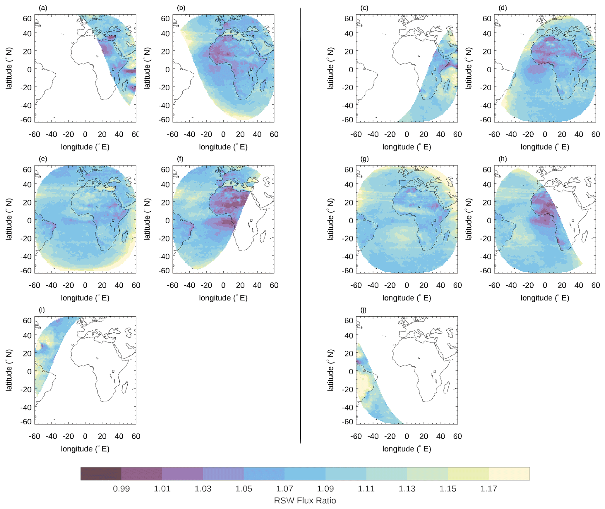
Figure 4 GERB and GERB-like RSW ratios of the monthly hourly mean at the 1° latitude–longitude scale for June 2009 in the two left-hand columns (a, b, e, f, i) and for December 2009 in the two right-hand columns (c, d, g, h, j) for 04:30 (a and c), 08:30 (b and d), 12:30 (e and g), 16:30 (f and h), and 20:30 (i and j) UTC.

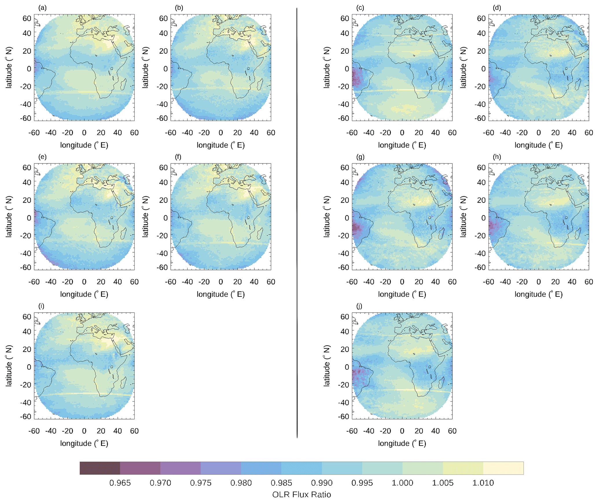
Figure 5 As in Fig. 4 but for the GERB and GERB-like OLR ratio for June 2009 in the two left columns (a, b, e, f, i) and December 2009 in the two right columns (c, d, g, h, j) for 04:30 (a and c), 08:30 (b and d), 12:30 (e and g), 16:30 (f and h), and 20:30 (i and j) UTC.

The ratios shown in Figs. 4 and 5 illustrate both a global bias between the two sets of fluxes and angularly dependent effects that manifest differently according to scene type. For RSW, the ratio between the GERB and GERB-like fluxes generally varies between 0.95 and 1.2. Variations occur with viewing and solar angles and thus with both location and time of day and, more subtly, the time of year associated with the variation in the solar zenith angle. The lowest RSW ratios tend to occur at larger solar zenith angles over land. The highest RSW ratios occur over the ocean and are mostly at larger solar zenith angles, especially when combined with large viewing zenith angles. For OLR the ratios are generally less extreme than RSW, with the lowest values of around 0.97 observed towards the edge of the GERB region at the largest viewing zenith angles for the coldest scenes. The fixed viewing geometry of the geostationary platform means that viewing zenith angle effects correspond to fixed locations. The diurnal variation in the GERB : GERB-like OLR ratio is small and is associated with marked changes in scene, e.g., the daily heating of the land, seen most significantly over desert regions such as the Sahara. Similarly, seasonal variations in the OLR ratio are associated with scene variations such as the seasonal variation in the positioning of the Intertropical Convergence Zone (ITCZ) and changes to solar-induced land heating.

Figures 4 and 5 show that the ratio between the GERB and GERB-like fluxes does indeed exhibit a variety of expected variations between the two datasets, with strong angular and scene-dependent patterns in the ratio of the fluxes dominating. However, we find that the day-to-day variation in the overall bias between the two datasets (not shown) manifests at a much lower level in both OLR and RSW and is difficult to distinguish from the combined effect of scene-dependent bias and day-to-day variation in scene make-up. If adjusting by the GERB : GERB-like ratio calculated at the monthly hourly mean 1° longitude–latitude scale can provide a good match between the GERB and GERB-like fluxes at the daily hourly scale, then the latter could be used to replace missing days of GERB data. Figure 6 displays the average and range of the mean and standard deviation of the individual daily hourly 1° longitude–latitude GERB − GERB-like difference distributions, as a function of UTC hour, before and after adjustment of GERB-like. Results are shown for RSW (left panels) and OLR (right panels) and summarize the individual distributions of the 1° longitude–latitude differences for each hour of every day where GERB and GERB-like data are available, as long as there are no more than 22 missing days in the month. By definition, adjustment by the monthly ratio removes the monthly mean bias, and the shift in the average value of the daily error distribution mean to around zero is expected. However, the reduction in the range of mean values after correction shows that the mean bias at the daily hourly level is consistently reduced by the monthly correction to less than a few Watts per square metre. Similarly, the reduction in the standard deviations shows that, despite day-to-day variations in meteorology, a correction derived at the monthly scale significantly reduces the range of errors seen at the daily hourly 1° longitude–latitude scale, with the standard deviations decreasing from averages of 10 to 4.6 W m⁻² in RSW and 2.2 to 1.7 W m⁻² in OLR. These results demonstrate that a single monthly hourly correction applied at the 1° longitude–latitude scale significantly improves the fidelity between the GERB-like and GERB fluxes at the daily hourly scale.

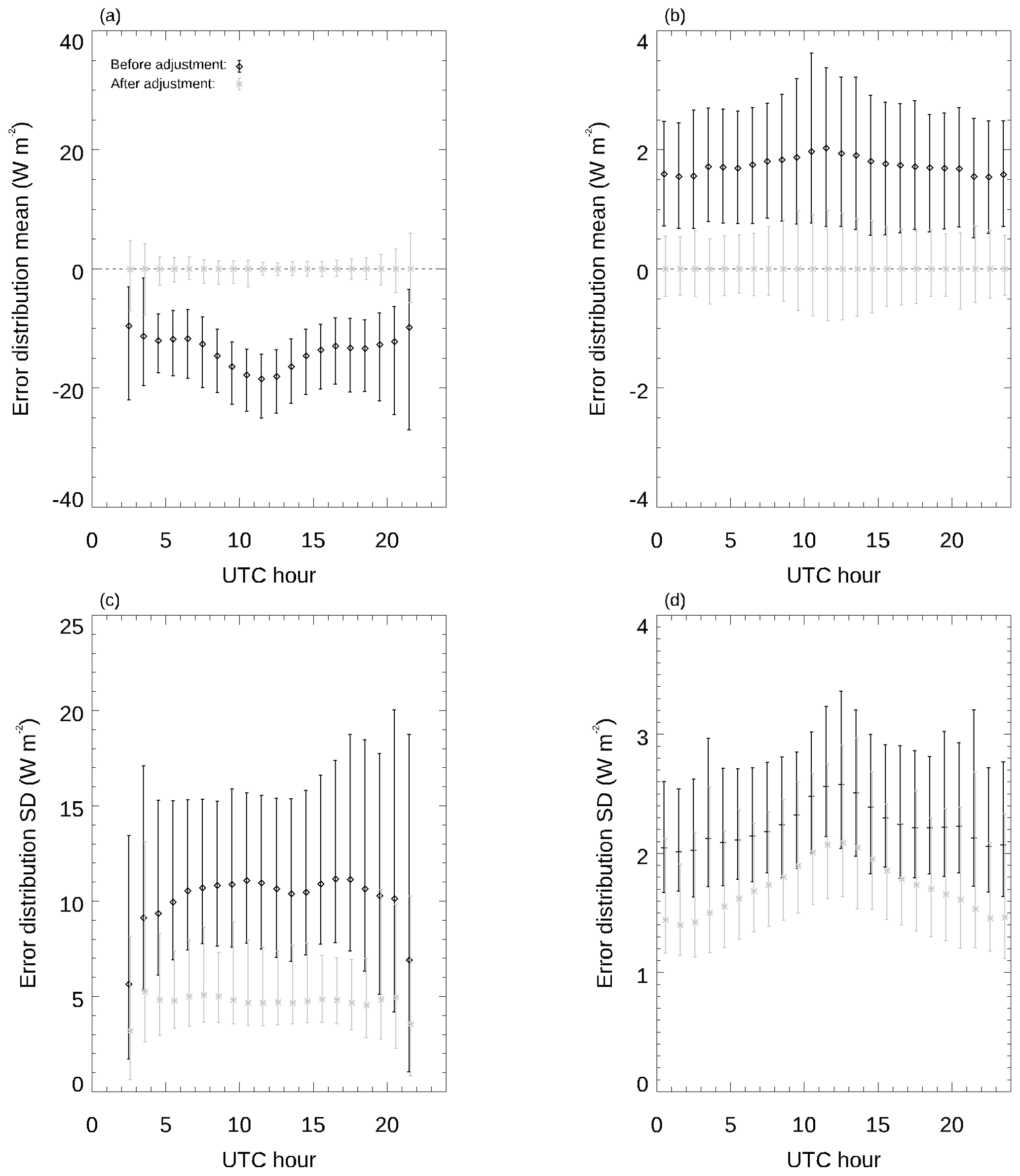
Figure 6 Summary statistics for the GERB-like − GERB difference before (black) and after (grey) adjustment of GERB-like by the monthly hourly ratio. Points indicate the average and the bars the range of these statistics over all the days at each hour. Results are shown as a function of UTC hour for RSW (panels a and c) and OLR (panels b and d) for the mean of the distribution (a and b) and the standard deviation (c and d). Times are on the half-hour in all the cases, but the plotting for the adjusted case is slightly offset on the x axis for clarity.

Thus, using corrected GERB-like data to fill missing hours of GERB data and then averaging over the month should improve the accuracy of the average. The required GERB-like correction is determined from the ratio between the GERB unfilled monthly hourly average and a corresponding GERB-like average calculated following the process outlined in Fig. 1, with the GERB-like data used to determine the average matched to the GERB data availability. This provides a monthly correction at the 1° longitude and latitude as a function of hour, which is then applied to daily hourly GERB-like data. The corrected GERB-like daily hourly data are used to fill in missing hours of the GERB record before averaging over the month to produce filled GERB Obs4MIPs products. This process is illustrated in Fig. 7, in which the 1° latitude–longitude GERB and GERB-like hourly and monthly hourly products, referred to as “hourly 1° × 1°” and “monthly–hourly 1° × 1°”, are derived following the steps outlined in Fig. 1.

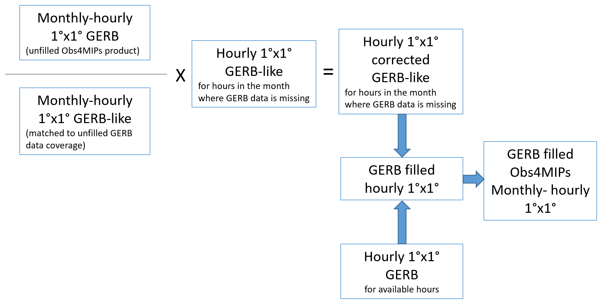
Figure 7 Schematic illustrating how GERB-like data are corrected and used with the GERB hourly data to produce filled Obs4MIPs products. The monthly to hourly 1° latitude–longitude products denoted here as 1° × 1° are produced using the steps illustrated in Fig. 1.

3 Evaluation of the GERB Obs4MIPs monthly hourly average products

Whilst the instantaneous GERB data, including the HR products, have been validated (Clerbaux et al., 2009; Parfitt et al., 2016), the effect of missing GERB observations on the fidelity of the GERB filled and unfilled Obs4MIPs averaged products needs additional consideration. As illustrated in Fig. 2, there are a significant number of monthly hourly averages where 1 d or more of GERB observations are missing. These gaps at the daily hourly scale, if left unfilled, result in errors in the Obs4MIPs monthly hourly averages due to the uncaptured day-to-day variability in the fluxes. Alternatively, if these gaps are filled, then the impact on the monthly hourly average of the difference between the proxy data used for filling and the GERB data they represent needs to be assessed. In this section we provide estimates of these error sources as a function of the number of missing days, considering the effect of both randomly distributed and consecutive missing days. In Sect. 3.1 we address how this impacts the V1.0 unfilled GERB Obs4MIPs products originally released, and in Sect. 3.2 we evaluate the error in the V1.1 averages after filling.

3.1 Impact of missing data on the fidelity of the unfilled GERB Obs4MIPs products

For the unfilled GERB Obs4MIPs products, the error in the monthly average due to missing data can be estimated by considering the effect of removing days from a month of data with complete, or nearly complete, coverage. Every UTC hour of the GERB-1 record with no more than 1 missing day during the month was used as a starting point for this analysis. This represents just over one-third of the data for the months not affected by the systematic outages around the equinoxes. It also provides good coverage of the diurnal cycle for each of these months.

In this analysis, we consider each of the “complete” or “nearly complete” monthly hourly averages to be the “true” value. Differences between these true values and the averages calculated after the removal of a selected number of days provide an estimate of the error due to missing data. The effect of removing between 1 and 12 d randomly distributed through the month was calculated for eight different realizations of the days chosen. The effect of removing between 2 and 22 consecutive days was also determined for three different patterns: all days missing at the start of the month, at the end of the month, and centred around the middle of the month.

Figure 8 displays example results for the removal of 3 randomly chosen days of data from the December 2012 11:30 UTC monthly hourly average. Four different realizations of the missing days are shown. The variation in the spatial distribution of the error (panels a to d for RSW and panels e to h for OLR) highlights the effect of the altered sampling. The largest differences in averages are seen for RSW in the more strongly illuminated summer hemisphere and are for the most part associated with the averaging of synoptic variability at higher latitudes. Notable errors are also present in other regions, which exhibit significant day-to-day variability in cloud coverage and/or properties, such as deep convective regimes over southern Africa. For both OLR and RSW, the detail of the spatially resolved errors varies for each of the realizations, depending on the meteorology on the individual days removed. However, the overall distribution of errors shown in panel i for RSW and panel j for OLR is relatively stable from realization to realization. For both OLR and RSW, the distributions are relatively symmetrical about the mean, which is close to zero. As might be anticipated from the spatial error patterns, the spread in the error is significantly larger for RSW than for OLR, with the associated standard deviations between 3.5 and 4 times higher for the former. We will use the mean and standard deviation of the error distribution as summary statistics for interpreting the change in the errors as a function of number of days missing, time of day, and month.

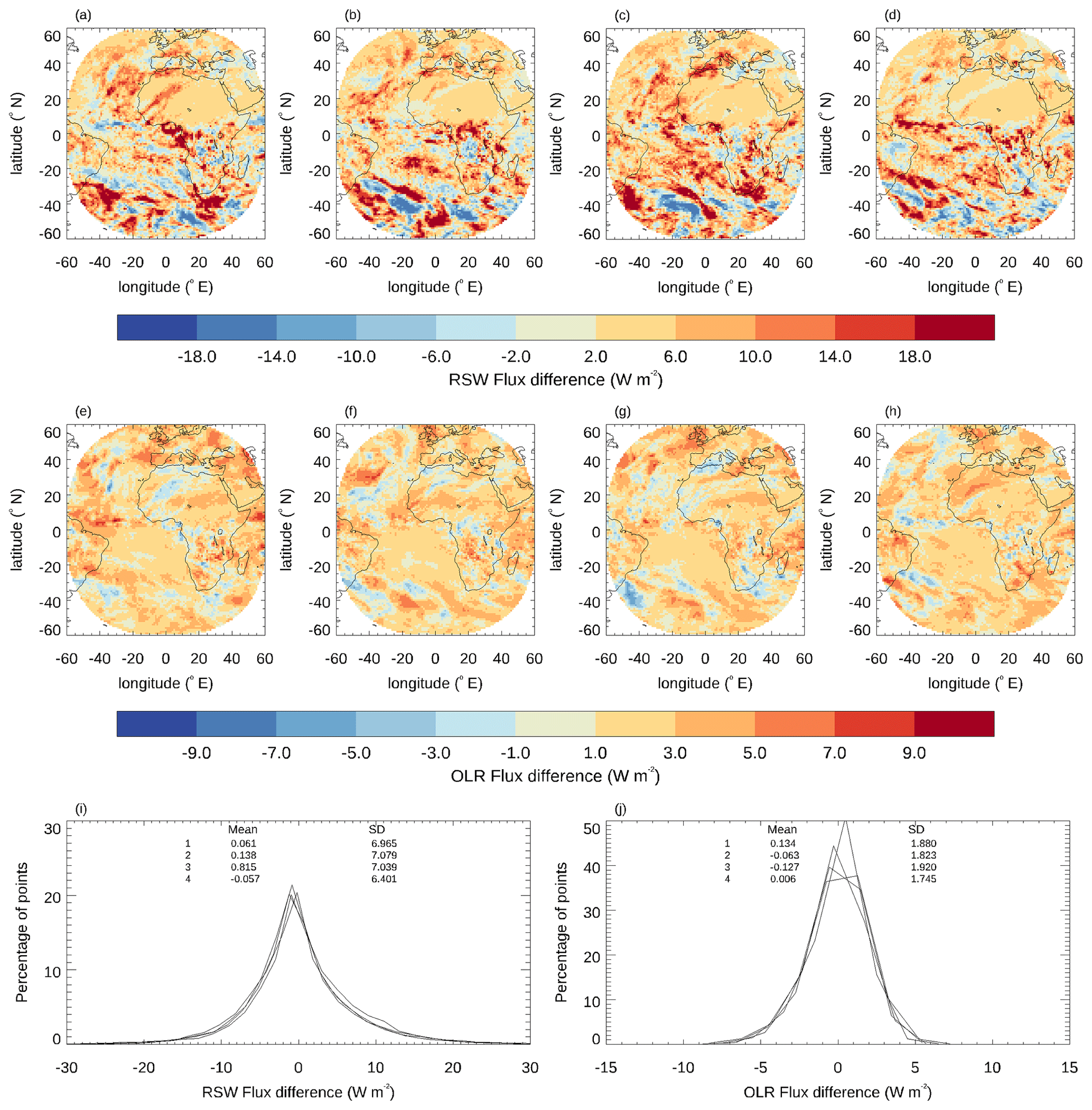
Figure 8 Impact on the 1° latitude–longitude monthly hourly mean fluxes of removing 3 randomly chosen days of data from December 2012 at 11:30 UTC. The results for four different random realizations of the days removed are shown spatially resolved for RSW in panels (a), (b), (c), and (d) and for OLR in panels (e), (f), (g), and (h). The corresponding distributions of the flux difference are shown for RSW and OLR in the bottom panels (i) and (j), respectively, with the mean and standard deviation in each of the four cases also displayed.

Considering the results for all the months and times of day used in this analysis, we find that, for OLR, systematic variations in the standard deviation and mean of the resulting error distribution, both seasonally and diurnally, are small and difficult to distinguish from the variability resulting from the choice of days. Seasonal variation in the error distribution is also negligible for RSW, aside from a small reduction in variability in the standard deviation and a very slight reduction in its value for July. This is associated with an increasingly dominant contribution from the Sahara, which has low day-to-day variability. However, there is a notable diurnal signal in the standard deviation of the RSW error distribution. Even when only calculated over the locations which are not at twilight or nighttime at any point in the month at that hour, the standard deviation, which is relatively stable between 10:30 and 15:30 UTC when there is a high level of solar illumination, drops steadily for earlier and later times of day, due to the overall reduction in the incoming solar flux. Results for hours earlier than 04:30 and later than 19:30 UTC are more unpredictable and generally noisy as there are typically less than 20 % of the full number of points represented in the statistics due to the limited portion of the disc illuminated at these times. Thus, for RSW, combining the results for all the months and for the hours 10:30 to 15:30 UTC gives an indication of errors at the height of the disc illumination. Errors at 04:30 and 19:30 UTC represent the error distribution for the low-illumination case, where there are still a sufficient number of points illuminated to obtain reasonable statistics.

Figure 9 summarizes the expected monthly hourly mean error due to missing data at the 1° scale, in terms of the standard deviation and mean of the error distribution for both randomly and systematically removed days. The results show that, on average, the mean and standard deviation increase roughly linearly as the number of missing days increases. The variability in the standard deviation and mean also increases as the number of missing days increases, but in a less regular manner. For the 10:30 to 15:30 UTC time range the standard deviation of the RSW error distribution increases rapidly as the number of missing days increases, exceeding 10 W m⁻² for some cases, with 4 or more consecutive missing days or 5 or more missing days randomly distributed through the month. The corresponding standard deviation which is exceeded for OLR in these cases is 3 W m⁻². For the mean of the error distribution, which is the overall image bias due to the missing data, individual realizations can see increasingly large biases as the number of missing days increases. When consecutive days are removed, the bias may exceed 2 W m⁻² for RSW and 1 W m⁻² for OLR for as few as 3 or 4 missing days for some of the cases.

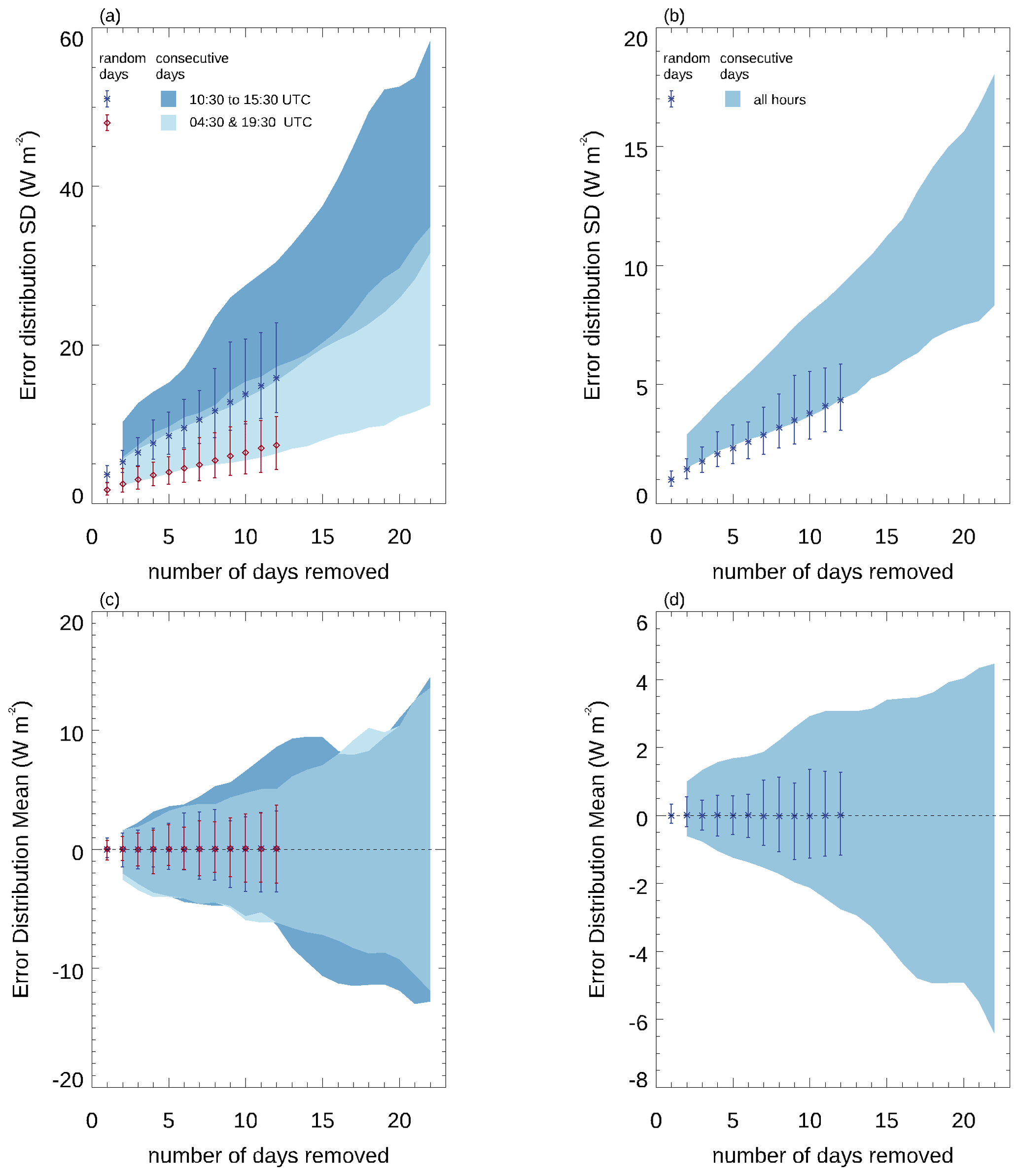
Figure 9 Summary statistics for the error distribution in the monthly hourly mean 1° latitude–longitude fluxes due to missing days. The standard deviation (panels a and b) and the mean (panels c and d) of the error distributions are shown as a function of the number of days removed for the RSW (a and c) and OLR (b and d) fluxes. The average and range over the realizations and months are shown for days removed and chosen at random as points with bars. The corresponding range for points systematically removed from various points in the month is shown as the shaded regions. For RSW, results are shown separately for the UTC hours 10:30–15:30, representing high solar illumination of the GERB region and for 04:30 and 19:30 combined, representing low solar illumination. The OLR results are shown for all the times together.

To avoid averages with unacceptably large errors, monthly hourly averages are only provided for the V1.0 unfilled GERB Obs4MIPs release when there are 5 or fewer missing days of data in the month for that hour. This means that the V1.0 GERB Obs4MIPs monthly hourly data are limited to the hours and months shaded in white or turquoise in Fig. 2 (a total of 645 monthly hourly averages), with the hours of each month shaded yellow or grey not provided to users for these products.

3.2 Fidelity of the filled GERB Obs4MIPs products

Whilst the improvement in the correspondence between the GERB and GERB-like daily hourly fluxes after adjustment with the monthly hourly ratio discussed in Sect. 2.3 is encouraging, these results are not quite representative of the situation in the case of missing GERB data. In this case the monthly hourly ratio derived from incomplete GERB and corresponding GERB-like fluxes will need to be used to correct GERB-like fluxes that are not included in that average. Thus, for the adjusted GERB-like fluxes to be useful for filling missing GERB data, it needs to be shown that rescaling by a monthly hourly average ratio derived from incomplete data can sufficiently improve the GERB-like fluxes at the daily to hourly 1° scale for the missing periods.

Analogously to the approach used in Sect. 3.1, starting with all the hours of the record with no more than 1 missing day of GERB data in a month, we determine the effect of removing increasing amounts of GERB data and replacing them with GERB-like data scaled by the monthly hourly ratio. In each case we match the data coverage for both GERB and GERB-like; i.e., corresponding points are removed from both data records before calculating the monthly hourly means and the associated ratio. As for the unfilled average comparison described in Sect. 3.1, the error due to filling can then be estimated from the difference between the resulting filled average and the average calculated from the GERB data alone before any data were removed.

Figure 10 summarizes statistics of the residual error at the monthly hourly average 1° latitude–longitude scale for the filled data. It can be directly compared to Fig. 9, which shows the equivalent results for the unfilled averages. Comparing the two figures shows that filling the missing days of GERB fluxes with their scaled GERB-like equivalents before calculating the monthly hourly average reduces both the mean and standard deviation of the error in the monthly hourly average at the 1° scale by more than a factor of 10 in all cases. Given these improved statistics, we implement this filling approach to produce our filled GERB Obs4MIPs product and use it in the next section to perform an initial evaluation of climate model performance. We note that the level of error reduction is retained even when there are up to 22 d systematically missing, and thus we are also able to reinstate the months of February and August in the filled record. Therefore, filled GERB monthly hourly Obs4MIPs products can be provided to users for all hours of the month that are not shaded grey in Fig. 2, with the error associated with filling bounded by the values shown in Fig. 10. This results in 1030 monthly hourly averages available to users of the V1.1 filled GERB Obs4MIPs products compared to the 645 for the V1.0 unfilled products.

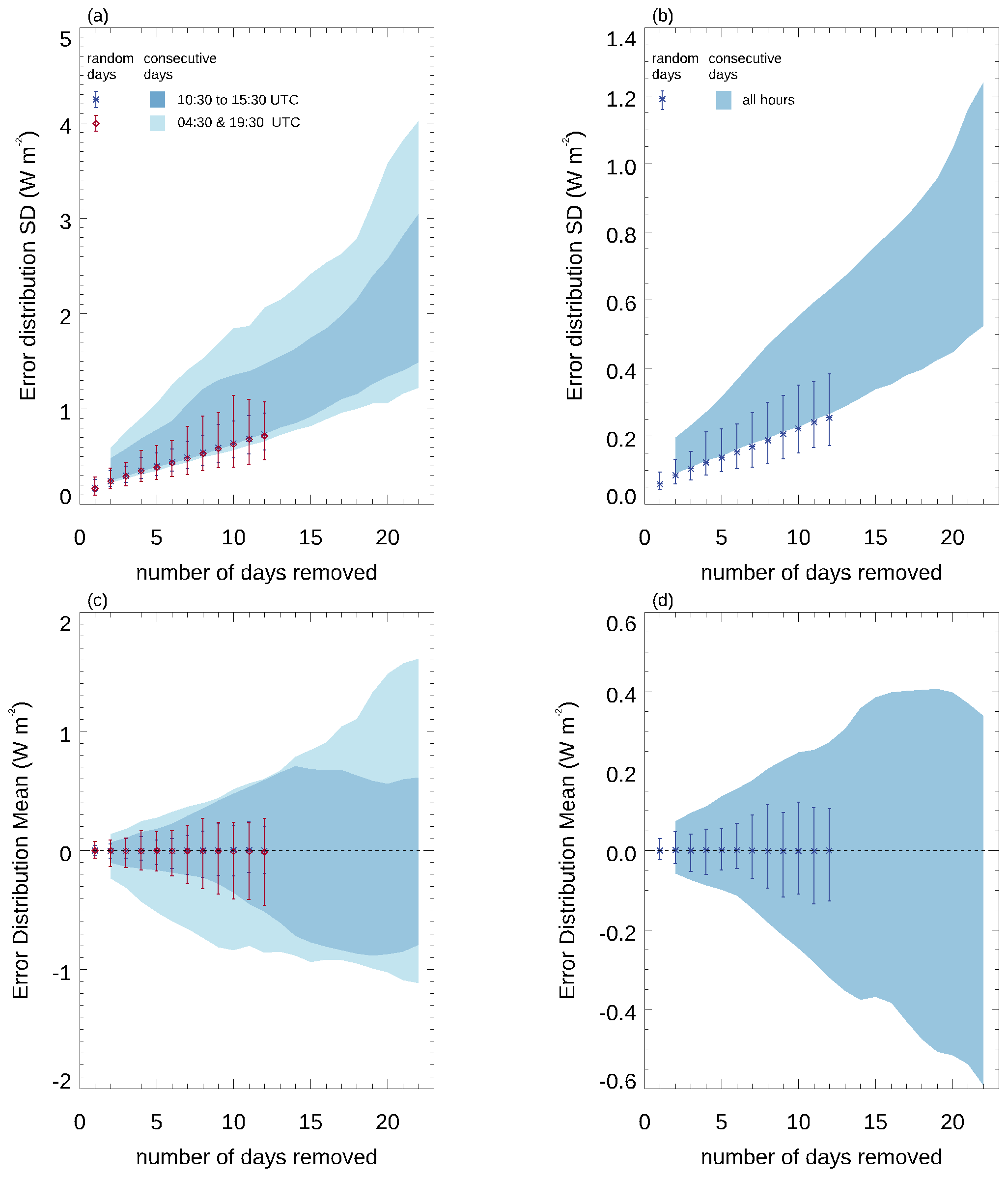
Figure 10 As in Fig. 9 but for the error distribution in the monthly hourly mean 1° latitude–longitude fluxes due to filling missing days with scaled GERB-like data as described in the main text. Note the change in the y-axis scales compared to Fig. 9.

4 Application of the GERB Obs4MIPs filled product to climate model evaluation

TOA radiative fluxes are routinely used as an evaluation metric for climate model performance, with model parameters often tuned to produce a realistic radiation budget. This is typically performed at a relatively coarse temporal and spatial scale (monthly or global annual means), which has the potential to mask compensating errors. A more stringent test, at least at the process level, compares temporally resolved fluxes. This type of comparison has also been recognized as potentially insightful for assessing cloud feedback (Webb et al., 2015) and has led to a limited number of modelling centres starting to produce and archive monthly hourly mean TOA radiative fluxes from Atmospheric Model Intercomparison Project (amip, Gates, 1992) runs. Here we compare such fluxes, as simulated by two versions of the climate configuration of the Hadley Centre's Global Environmental Model HadGEM3, with the V1.1 filled GERB Obs4MIPs product. Concentrating on two cloud regimes, we show how the diurnally resolved fluxes can complement other observationally based evaluations and provide unique insights into the model fidelity.

4.1 HadGEM3 configurations and simulation description

Our analysis concerns historical amip simulations of two different Global Coupled model configurations of HadGEM3 (GC3.1 and GC5.0). Both model configurations consist of atmosphere, land, ocean, and sea ice sub-components, have 85 vertical layers, and are run at N96 (1.875° longitude by 1.25° latitude) horizontal resolution. The amip simulations are forced with observations of sea surface temperatures, sea ice cover, and historical forcings (Eyring et al., 2016).

GC3.1 is the configuration that underpinned the United Kingdom's contribution to CMIP6 (Williams et al., 2018; Mulcahy et al., 2018; Walters et al., 2019). The most recent configuration (GC5.0) has not been documented yet but includes three changes affecting cloud that are particularly relevant to our analysis. A prognostically based convective entrainment linked to surface precipitation which introduces memory into the convection scheme is expected to improve the representation of the diurnal cycle of convection over land. A new bimodal diagnostic cloud fraction scheme (Van Weverberg et al., 2021a and b) and a reformulation of the “cloud erosion” term (Morcrette, 2012) in the large-scale cloud scheme (Wilson et al., 2008a and b) are expected to improve the realism of cloud evolution and increase the amount and optical thickness of low-level cloud, particularly in the sub-tropics and at the lower mid-latitudes.

Monthly mean diurnal cycles of TOA radiative fluxes (all-sky and clear-sky) are produced for the entire length of the amip experiment. The radiative fluxes are hourly means centred, as in the observations, on the half-hour, and the monthly mean diurnal cycle is constructed by averaging each UTC hourly mean over the entire month. These diagnostics were requested for the amip experiment of phase 3 of the Cloud Feedback Intercomparison Project (Webb et al., 2017). The HadGEM3 OLR diagnostics used in this study differ from those submitted to CFMIP3. The OLR diagnostics submitted to CFMIP3 contain a correction that accounts for the surface temperature adjustment by the boundary layer scheme in model time steps between radiation time steps. This OLR diagnostic adjustment is introduced to conserve energy, but it significantly distorts the diurnal cycle of OLR (its impact on daily and longer time averages is very small). Given that this OLR correction is purely diagnostic (i.e. it does not affect the model evolution) and was not designed to work on sub-daily timescales, here we have used OLR without this correction.

4.2 Model evaluation

For the purposes of highlighting the utility of the V1.1 GERB Obs4MIPs product, we focus on two cloud regimes, i.e. marine stratocumulus and deep convection. Improving the representation of sub-tropical stratocumulus has been a focus of climate modellers for some time due to its importance in determining global cloud feedback (e.g. Bony and Dufresne, 2005). In general, models have tended to simulate too little marine stratocumulus, with what is present being too bright (e.g. Nam et al., 2012). In the multi-annual mean, Williams and Bodas-Salcedo (2017) report good agreement between GC3.1 and CALIPSO height–frequency statistics over stratocumulus but with a distribution that shows too few moderately optically thick clouds, which is compensated for by too many optically thick clouds. Comparisons with CERES–EBAF monthly mean TOA RSW fluxes imply that this translates into stratocumulus decks that are too reflective.

Deep convective regions continue to present a challenge, at least in part because of the scale at which convection is typically parameterized in global climate models (e.g. Guichard et al., 2004; Hohenegger and Stevens, 2013; Christopoulos and Schneider, 2021). Although improvements have been made (e.g. Stratton and Stirling, 2012), a persistent issue over land is that convective clouds tend to rain out too early, leading to too little cloud in the late afternoon to evening, when deep convection (and precipitation) typically peaks in observations (e.g. Yang and Slingo, 2001; Tan et al., 2019). Such issues persist to some extent even in higher-resolution simulations (e.g. Watters et al., 2021). Given the temporal resolution of the GERB Obs4MIPs product, it is ideally suited to investigating whether adjustments to the parameterizations that affect the convective invigoration and life cycle in GC5.0 are having a beneficial impact in terms of the TOA energy budget.

We begin with a qualitative comparison of the overall monthly means to provide context for the diurnally resolved regional comparisons that follow. Figure 11 a and b show decadal average monthly mean January RSW fluxes as simulated by GC3.1 and GC5.0 over the region 60° S–60° N and 60° E–60° W. V1.1 GERB Obs4MIPs RSW fluxes are shown in panel (c), in this case averaged over the 5 years of GERB-1 January observations. The corresponding information for June is shown in panels (d)–(f) with, in this case, 6 years of observations available for averaging. Broadly speaking, the simulations capture the patterns seen in the observations, including the seasonal shift in the positioning and strength of features such as the ITCZ and stratocumulus decks off Angola and Namibia. There are differences: during the summer hemisphere, GERB shows significantly higher RSW fluxes over the highest latitudes. It is noticeable that GC5.0 also tends to be brighter than GC3.1 in those regions. GC5.0 also appears to show more extensive, brighter marine stratocumulus off the western African coast in both seasons compared to GC3.1.

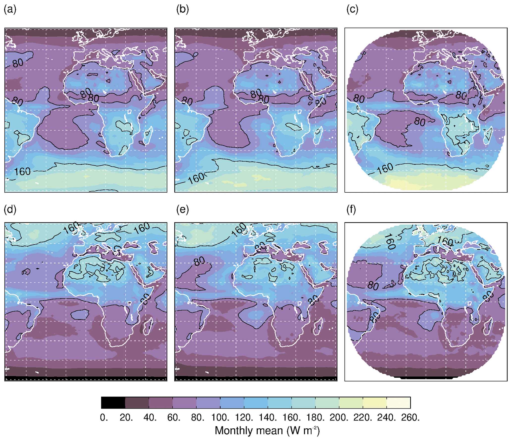
Figure 11 Monthly average TOA RSW fluxes for January in the top row (a, b, and c) and for June in the bottom row (d, e, and f) from GC3.1 (left panels: a and d), GC5 (middle panels: b and e), and V1.1 GERB Obs4MIPs (right panels: c and f). The simulated fluxes are a decadal mean (2000–2009). GERB fluxes are averaged over the duration of the GERB-1 observations.

The information equivalent to Fig. 11 is shown in Fig. 12 for OLR fluxes. In this case, the most obvious differences between the two HadGEM3 simulations are located in regions of tropical deep convection. In June, GC5.0 appears to shift the peak of convection within the ITCZ further east. In January, the centres of deep convection over Brazil and central southern Africa are both strengthened in GC5.0 relative to GC3.1. Visually, both changes appear more in line with the GERB observations, although the intensity of land convection still appears greater in the observations.

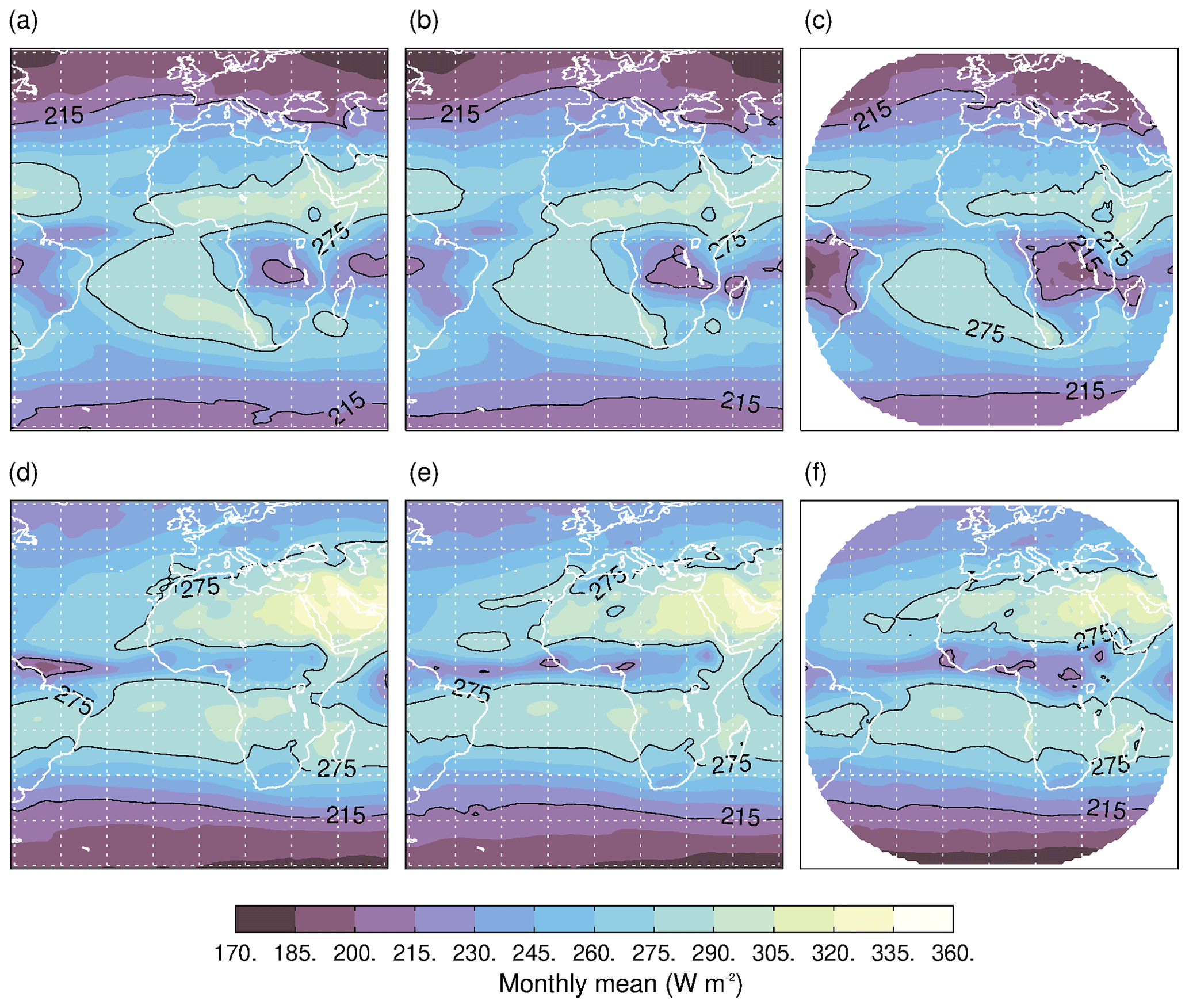
Figure 12 As in Fig. 11 but for OLR fluxes.

To provide a more quantitative analysis, we define two seasonally dependent latitude–longitude boxes encompassing the south-eastern Atlantic stratocumulus deck and African deep convection. Table 1 shows the multi-year June and January monthly mean fluxes obtained from both sets of simulations and from GERB in these regions. We note that shortening the period of averaging in the simulated datasets to be commensurate with the length of the GERB record makes a difference of, at most, 3 W m⁻² in the mean fluxes.

Table 1 Multi-year June and January monthly mean RSW and OLR fluxes over regions characterized by marine stratocumulus and deep convective cloud as observed by GERB and simulated by the two configurations of HadGEM3 outlined in the main text.

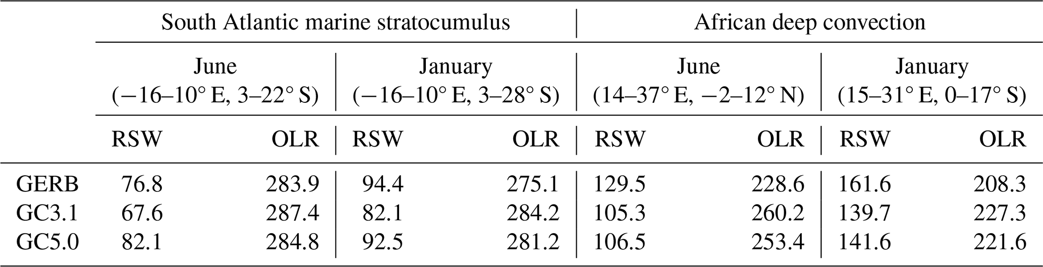
Over the stratocumulus region, Table 1 reinforces the qualitative impression from Figs. 11 and 12, with the change in the HadGEM3 configuration resulting in a distinct brightening in both June and January. In June, the degree of brightening means that the mean RSW flux exceeds that measured by GERB, whereas in January the increment is still insufficient to reach the level of the observed fluxes. As might be anticipated given typical stratocumulus altitudes, the impact on the OLR fluxes is less marked but is consistent between the months, decreasing by order 3 W m⁻². In concert, these two results imply an enhanced cloud fraction, optical depth, or both in the GC5.0 configuration.

The largest differences between the two sets of simulated fluxes over deep convection are realized in OLR. Moving from GC3.1 to GC5.0 results in a reduction in OLR of order 7 W m⁻² in both months, while a small increase of less than 2 W m⁻² is seen in the corresponding RSW fluxes (Table 1). These changes move the GC5.0 fluxes towards the observations, but there is still a notable overestimate in OLR flux and a corresponding underestimate in RSW flux, particularly in June, which is consistent with the visual impression of “missing” land convection in the simulations during this month (Fig. 12).

To understand the reasons behind the changes in the model fluxes in both regions, we use diagnostics produced by version 1.4 of the CFMIP (Cloud Feedback Model Intercomparison Project) Observational Simulator Package (COSP; Bodas-Salcedo et al., 2011). In particular, we use vertical profiles of cloud fraction of the Cloud–Aerosol Lidar and Infrared Pathfinder Satellite Observation simulator (CALIPSO) and International Satellite Cloud Climatology Project (ISCCP) histograms of cloud fraction in intervals of cloud top pressure (CTP) and cloud optical thickness (τ). The CALIPSO and ISCCP simulators are documented in Chepfer et al. (2008) and Klein and Jakob (1999), respectively.

Figure 13 illustrates these diagnostics for January. The results for June are qualitatively similar. GC5.0 shows a significant increase in cloud fraction in the stratocumulus region (Fig. 13a), with clouds also being optically thicker (Fig. 13c and e). These two changes contribute to the increase in RSW described above. In the deep convection region, GC5.0 shows an enhanced cloud fraction at high altitudes, coupled with a lower cloud top height (Fig. 13b). The impact of these two changes on OLR will partially cancel out. However, GC5.0 also shows optically thicker clouds (Fig. 13d and f). The combined increase in cloud fraction and optical thickness leads to a reduction in OLR in GC5.0 compared to GC3.1 (Table 1), despite the reduction in cloud top height.

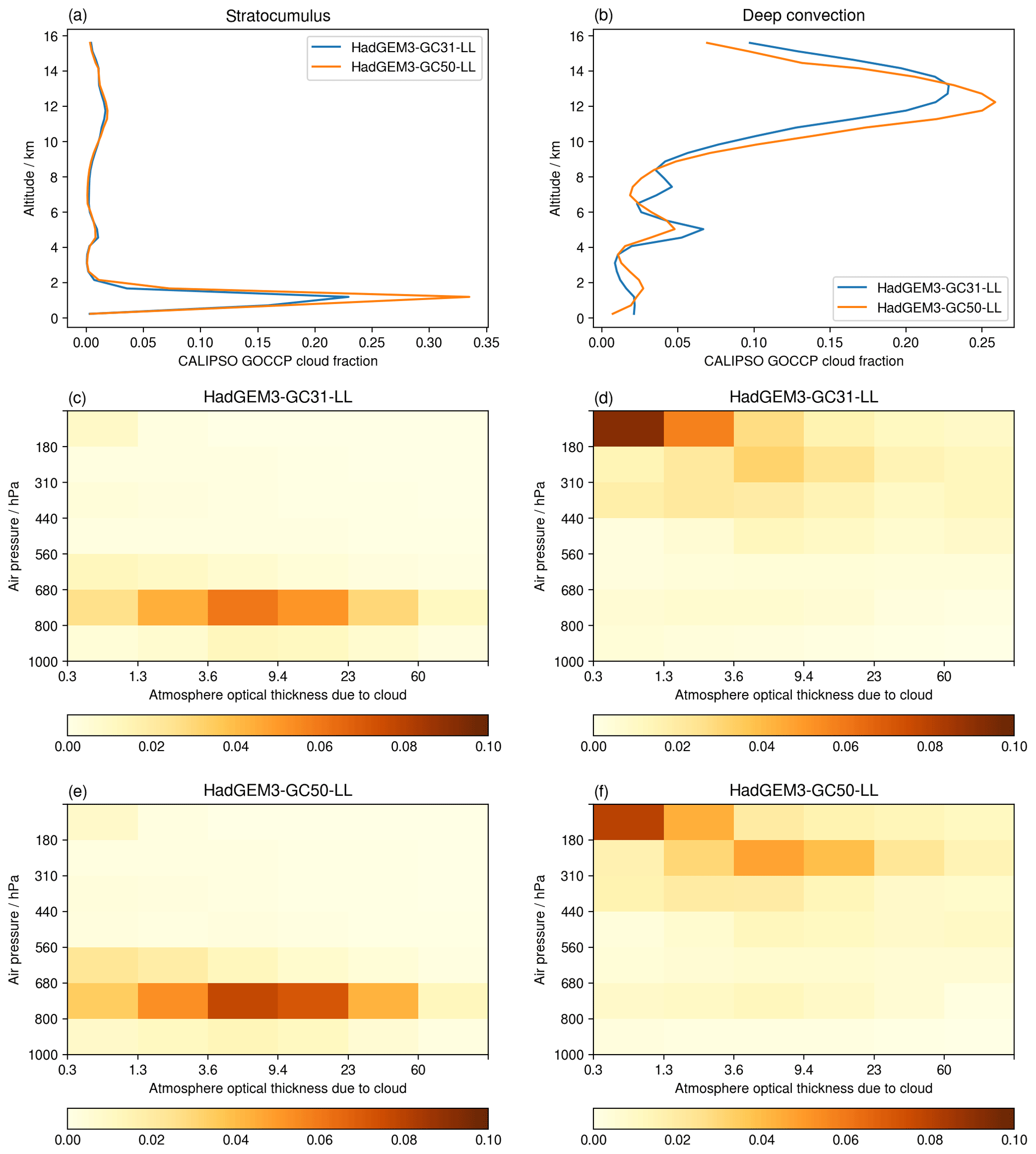
Figure 13 Multi-annual monthly average cloud fraction for January. Vertical profiles of the COSP/CALIPSO cloud fraction (a and b) and the COSP/ISCCP CTP-τ histograms of the cloud fraction (c to f). Panels (a), (c), and (e) show plots for the stratocumulus region and panels (b), (d), (f) those for the deep convection region.

Utilizing the diurnally resolved V1.1 GERB Obs4MIPs fluxes, we analyse these results further by decomposing them as a function of time of day. Figure 14 shows the regional hourly monthly mean RSW fluxes from each HadGEM3 configuration for each individual year of the simulation as well as the 10-year model mean over the stratocumulus regions. Superposed in colour are the GERB Obs4MIPs fluxes for 2007–2012. Figure 15 shows the equivalent information for OLR fluxes over the regions of deep convection.

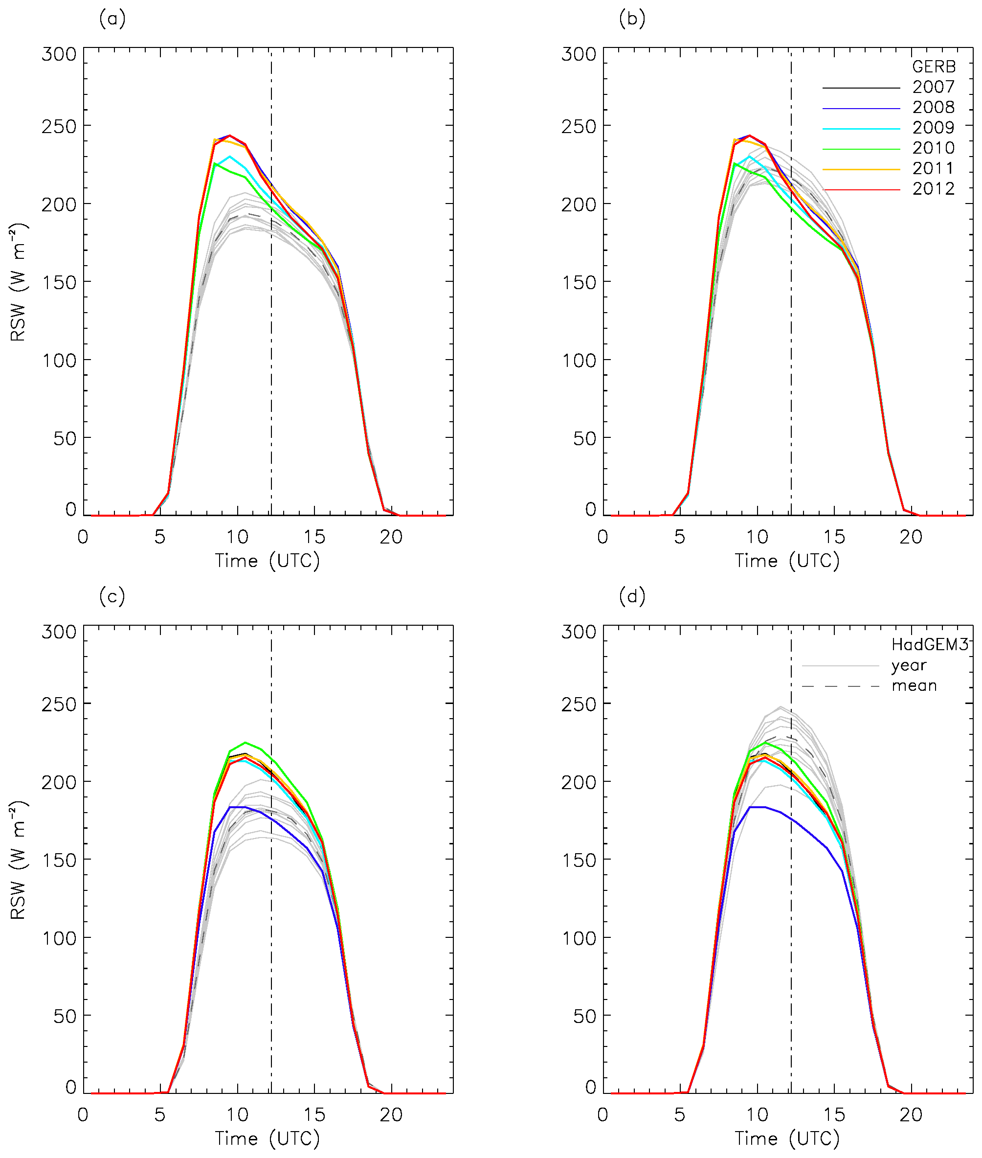
Figure 14 Monthly hourly mean RSW fluxes over the marine stratocumulus regions identified in Table 1 for January (a, b) and June (c, d). Coloured lines show the GERB Obs4MIPS fluxes for each year of the GERB observations. Solid grey lines show the simulated fluxes for each simulation year and the dashed grey line the 10-year mean for the HadGEM3-GC3.1 (a, c) and HadGEM3-GC5.0 (b, d) configurations. Dot-dashed vertical lines show the approximate timing of local noon.

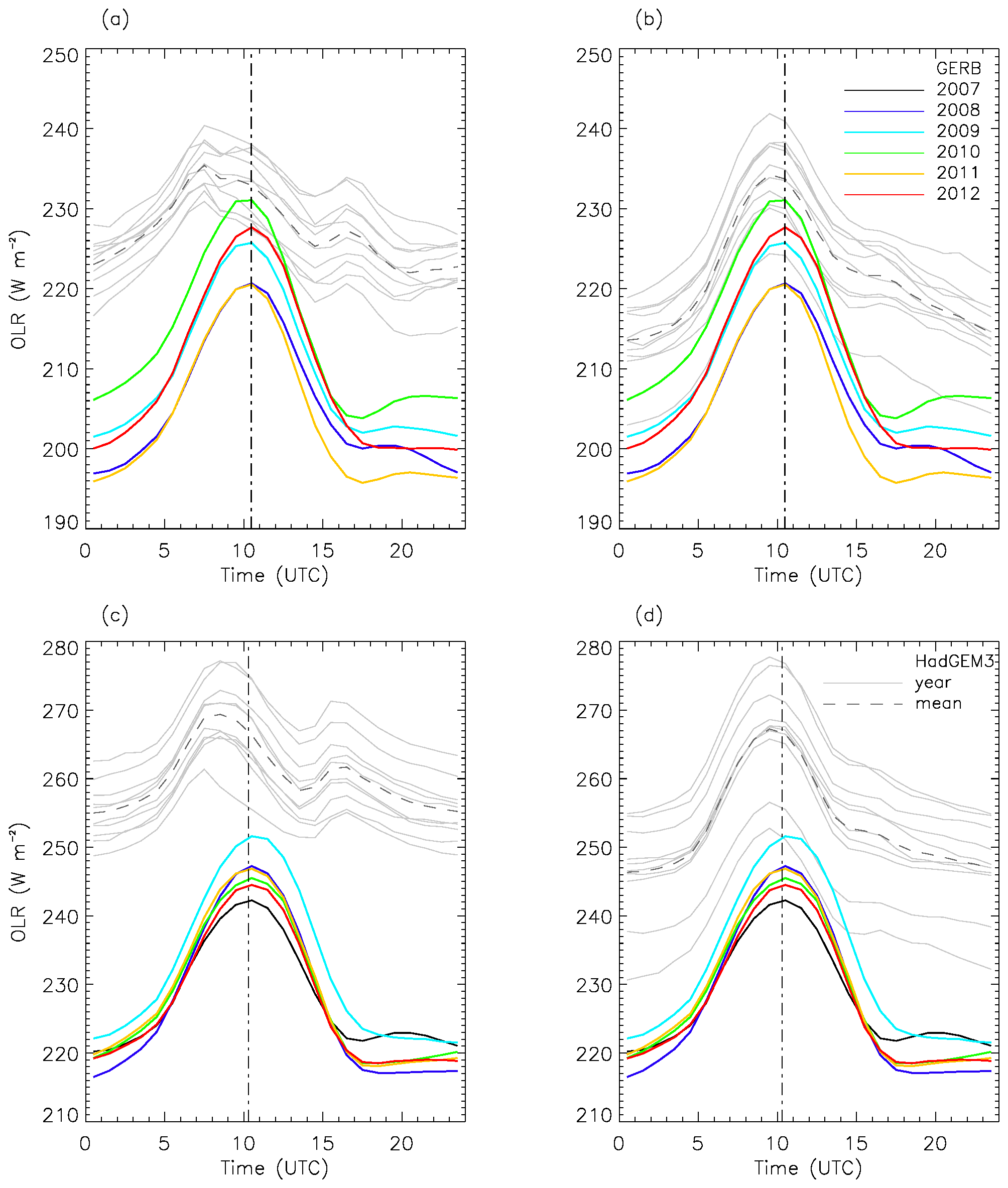
Figure 15 As in Fig. 14 for monthly hourly mean OLR fluxes over the deep convective regions identified in Table 1 for January in the top row (a and b) and for June in the bottom row (c and d). Simulations for GC3.1 are shown in panels (a) and (c) and for GC5.0 in panels (b) and (d).

Focusing on Fig. 14 first, the observations show the classic signature of stratocumulus development and thickening in the morning prior to decay through the afternoon, manifested as a clear asymmetry in the RSW fluxes around local noon (e.g. Gristey et al., 2018). This asymmetry is more pronounced in January than June. There is significant year-to-year variability in the magnitude of the observed fluxes (peak values can vary by up to 40 W m⁻²), but they all have this characteristic phasing. The degree of observed inter-annual variability is smaller in January than June – behaviour that is also captured in the model simulations. While the simulations do exhibit a diurnal asymmetry, they are unable to fully capture its observed magnitude. Similarly, although they show a constant diurnal phase from year to year, peak values for both model configurations are typically delayed by 1 h compared to the observations (Table 2). However, comparison of the GC3.1 and GC5.0 configurations does reinforce the impression that, within these limitations, the latter is able to better capture the observed behaviour even if the improvement to the phasing between the configurations is slight.

Table 2 Amplitude and phase in multi-year June and January monthly mean RSW and OLR fluxes over marine stratocumulus and deep convective regions, as observed by GERB and simulated by the two configurations of HadGEM3. Amplitude, A, is defined as $A=\mathrm{Max}\left(x_{\mathrm{t}}-\stackrel{\mathrm{‾}}{x_{\mathrm{t}}}\right)$, where x_t is the RSW or OLR flux as a function of hour through the day, and phase is the time (UTC) at which the value of A is realized.

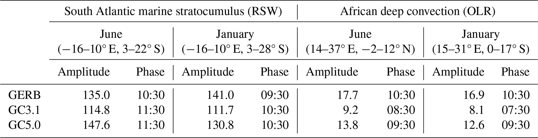
Turning to the deep convective regions (Fig. 15), the observed OLR fluxes show a spread over the years considered which reaches the order of 10–15 W m⁻². The phasing of the cycle changes between the 2 months, with the OLR fluxes reaching their maximum just after local noon in June and just before or at local noon in January. For both months the timing of the maximum is consistent from year to year, although there is marked inter-annual variation in the shape of the cycle towards late afternoon and evening, particularly in January. The corresponding simulated values from GC5.0 highlight an improved ability to capture the general shape of the diurnal cycle, with the removal of what appears to be a spurious secondary peak in the OLR fluxes in late afternoon in GC3.1. The timing of the OLR maximum is shifted later in GC5.0 by between 1 and 2 h and is more consistent with the observations, albeit still too early in the day. The amplitude of the cycle is also improved (Table 2). These improvements in the diurnal cycle are mainly driven by the introduction of the prognostic entrainment rate. Clearly, other issues remain: in June the fluxes are consistently too high, implying either missing convection or convection which is not vigorous enough. The inter-annual variability over the region is significantly higher than seen in the observations, which would be consistent with this interpretation. Both issues are present to a lesser extent in January. However, overall, the direction of travel from GC3.1 to GC5.0 is encouraging, particularly when viewed in a diurnally resolved comparison.

In climate models, the diurnal cycle of convection is typically evaluated using the diurnal cycle of precipitation (e.g. Stratton and Stirling, 2012). The remote sensing technology, spatio-temporal sampling, and retrieval algorithms used in the precipitation retrievals introduce substantial uncertainty into the timing of the maximum of precipitation in the mean diurnal cycle (Dai et al., 2007; Minobe et al., 2020). The GERB dataset presented here provides a very accurate description of the monthly mean diurnal cycle of the OLR and RSW fluxes, making it an excellent tool for the evaluation of the diurnal cycle of convection in models. It is worth noting that the minimum in OLR is delayed by around 3 h with respect to the maximum in precipitation in convective regions (Dai et al., 2007), and therefore a combination of radiation and precipitation diagnostics can provide a more detailed picture of the evolution of precipitation and the anvil cloud associated with the development of deep convection.

Table 3 Data characteristics of the GERB Obs4MIPs products.

5 Data availability

The V1.0 unfilled and V1.1 filled GERB Obs4MIPs OLR and RSW products presented in this paper are available from the Centre for Environmental Data Analysis (https://doi.org/10.5285/7aa17e66aaab4ece87064272b9f94e3a (Bantges et al., 2021a) and https://doi.org/10.5285/4fa633d24d104217a4c9d3fb3589f35d (Bantges et al., 2021b) for the V1.0 unfilled OLR and RSW and https://doi.org/10.5285/90148d9b1f1c40f1ac40152957e25467 (Bantges et al., 2023a) and https://doi.org/10.5285/57821b58804945deaf4cdde278563ec2 (Bantges et al., 2023b) for the V1.1 filled OLR and RSW). The datasets are also available from the Earth System Grid Federation.

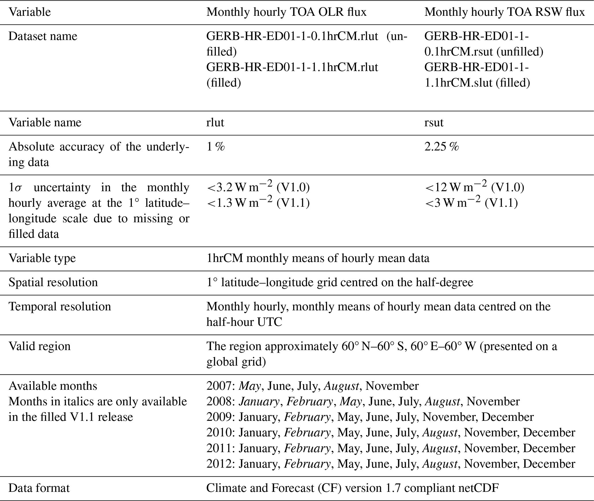
The characteristics of the GERB Obs4MIPs products are summarized in Table 3.

Model outputs used for the comparisons presented in Sect. 3 are available at https://doi.org/10.5281/zenodo.10101394 (Bodas-Salcedo, 2023).

6 Conclusions

The GERB Obs4MIPs products are specifically designed to enable the evaluation of the diurnal cycle in TOA radiation fluxes, as simulated by climate and Earth system models. This paper has described in detail how the GERB Obs4MIPs products are derived from the baseline GERB HR data to give monthly hourly mean OLR and RSW fluxes on a regular 1° latitude–longitude grid. Whilst the instantaneous GERB data have been fully evaluated and compared against the CERES products in previous comparisons (Clerbaux et al., 2009; Parfitt et al., 2016, Doelling et al., 2013, 2016), because of the relative prevalence of missing observations, which occur both randomly throughout the record and systematically around the equinoxes, particular attention has been paid in this study to the impact of missing data on the fidelity of averages. Our results show how estimates of the instantaneous broadband “GERB-like” fluxes from the SEVIRI narrowband instrument can be used to fill missing GERB data. A scaling factor is calculated from the ratio of the monthly hourly 1° latitude–longitude averages for the available GERB and matched GERB-like data and applied to the daily hourly GERB-like data. Using these scaled GERB-like fluxes to fill the missing GERB observations at the daily hourly scale before averaging significantly improves the fidelity of the monthly hourly averages when there are missing days of GERB data. For a given number of missing days, the residual uncertainty in the monthly hourly average at the 1° latitude–longitude scale due to filling is smaller by more than a factor of 10 than the error in the unfilled data due to missing days. Even when there is a substantial amount of systematic missing data, as is the case for GERB in the months of February and August every year, using the scaled GERB-like data to fill the missing periods leads to relatively small errors which are comparable to the error manifested in the unfilled dataset if just 1 d of data is missing. Using this method, V1.1 filled GERB Obs4MIPs products have been produced which provide greater coverage of the year and higher fidelity averages than the original V1.0 unfilled products.

We use the new V1.1 filled GERB Obs4MIPs products to perform a preliminary evaluation of two sets of amip-type simulations for the HadGEM3 climate model. The two sets of simulations differ in their atmospheric components, with the newer configuration implementing a prognostically based entrainment rate scheme, a bimodal cloud scheme within entrainment zones associated with strong temperature inversions, and improvements to the influence of dry air entrainment on cloudy grid boxes. At the monthly mean level, there are noticeable differences in TOA fluxes, with an overall brightening in the newer GC5.0 configuration and an apparent strengthening of convection. Although such changes would be evident in comparisons with existing radiative flux observations, further decomposing into the monthly hourly diurnal cycle allows insight into the amplitude and phasing of, in particular, different cloud regimes. Focusing on stratocumulus decks off south-western Africa and deep convection over Africa, the GERB Obs4MIPs product indicates that the monthly mean changes are consistent with an improved diurnal amplitude and, in the case of the convective region, phase in these regions. Discrepancies still remain: for example, the simulated RSW asymmetry seen over the stratocumulus deck is not as pronounced as in the observations and tends to be delayed by around 1 h compared to the observations, for both model configurations. Similarly, deep convection over Africa in boreal summer is too weak, and in both the winter and summer seasons it tends to occur slightly too early, resulting in an earlier simulated peak in OLR than seen in the observations. Tying these initial results to the behaviour of the underlying driving fields will be one avenue for future investigation.

We have shown that the GERB Obs4MIPs product is a very valuable complement to the traditional climatological averages of TOA radiation used for model evaluation. It provides a more direct connection with the model processes that control errors at both weather and climate timescales. Also, the fact that it is presented in a CF-compliant netCDF format makes it extremely user-friendly and ready to be incorporated into standard model evaluation tools like ESMValTool (Eyring et al., 2020).

Unfilled (V1.0) and filled (V1.1) GERB Obs4MIPs monthly hourly averages have been released as v1.7 CF-compliant netCDF products for the GERB-1 (Meteosat-9) observation period (May 2007 to December 2012). These are presented at 1° latitude–longitude resolution on a global grid with valid fluxes for the geographical region of approximately 60° N–60° S and 60° E–60° W. Users are recommended the V1.1 release for all applications. The V1.1 products are available for 8 months of the year (January, February, May, June, July, August, November, and December) for most of the released period. The underlying absolute accuracy of the GERB data is 1 % for OLR and 2.25 % for RSW, and additional errors due to filling missing data are estimated to be less than 1.3 W m⁻² for OLR and less than 3 W m⁻² for RSW in V1.1 monthly hourly averages at the 1° latitude–longitude scale. Obs4MIPs monthly hourly average products for the GERB-2 (Meteosat-8) period (May 2004 to February 2007) are currently in production using the V1.1 methods described here and are expected to be released soon. The short record and data quality issues affecting the GERB-3 (Meteosat-10) record (May 2015 to February 2018) as a result of various operational issues make it difficult to determine at this time whether these data will be suitable for similar treatment. However, Obs4MIPs products for the GERB-4 (Meteosat-11) period (May 2018 to February 2023) are expected to be produced once the underlying data have completed the full record calibration stability assessment that is currently underway.