the Creative Commons Attribution 4.0 License.
the Creative Commons Attribution 4.0 License.
 | 16 Sep 2024
Salinity and Stratification at the Sea Ice Edge (SASSIE): an oceanographic field campaign in the Beaufort Sea
Kyla Drushka
Elizabeth Westbrook
Frederick M. Bingham
Suzanne Dickinson
Severine Fournier
Viviane Menezes
Sidharth Misra
Jaynice Pérez Valentín
Edwin J. Rainville
Julian J. Schanze
Carlyn Schmidgall
Andrey Shcherbina
Michael Steele
Jim Thomson
Seth Zippel
As our planet warms, Arctic sea ice coverage continues to decline, resulting in complex feedbacks with the climate system. The core objective of NASA's Salinity and Stratification at the Sea Ice Edge (SASSIE) mission is to understand how ocean salinity and near-surface stratification affect upper-ocean heat content and thus sea ice freeze and melt. SASSIE specifically focuses on the formation of Arctic Sea ice in autumn. The SASSIE field campaign in 2022 collected detailed observations of upper-ocean properties and meteorology near the sea ice edge in the Beaufort Sea using ship-based and piloted and drifting assets. The observations collected during SASSIE include vertical profiles of stratification up to the sea surface, air–sea fluxes, and ancillary measurements that are being used to better understand the role of salinity in coupled Arctic air–sea–ice processes. This publication provides a detailed overview of the activities during the 2022 SASSIE campaign and presents the publicly available datasets generated by this mission (available at https://podaac.jpl.nasa.gov/SASSIE, last access: 29 May 2024; DOIs for individual datasets in the “Data availability” section), introducing an accompanying repository that highlights the numerical routines used to generate the figures shown in this work.
- Article
(18120 KB) - Full-text XML
-
Supplement
(107019 KB) - BibTeX
- EndNote


1.1 Background
Sea ice extent in the Arctic Ocean has declined dramatically over the past few decades. As a result of climate change, autumn ice advance is slower and occurs later, while summer ice retreat is faster and occurs earlier (Stroeve et al., 2014; Stroeve and Notz, 2018). The result is a lengthening open-water period each year, leading to changes in air–sea heat and momentum fluxes, the freshwater cycle, surface albedo feedback, primary production, and regional and global climate, as well as human and ecological health (Lannuzel et al., 2020). Understanding the dynamics that govern the spatial and temporal patterns of sea ice formation is critical to understanding and predicting the impacts of the changing Arctic cryosphere.
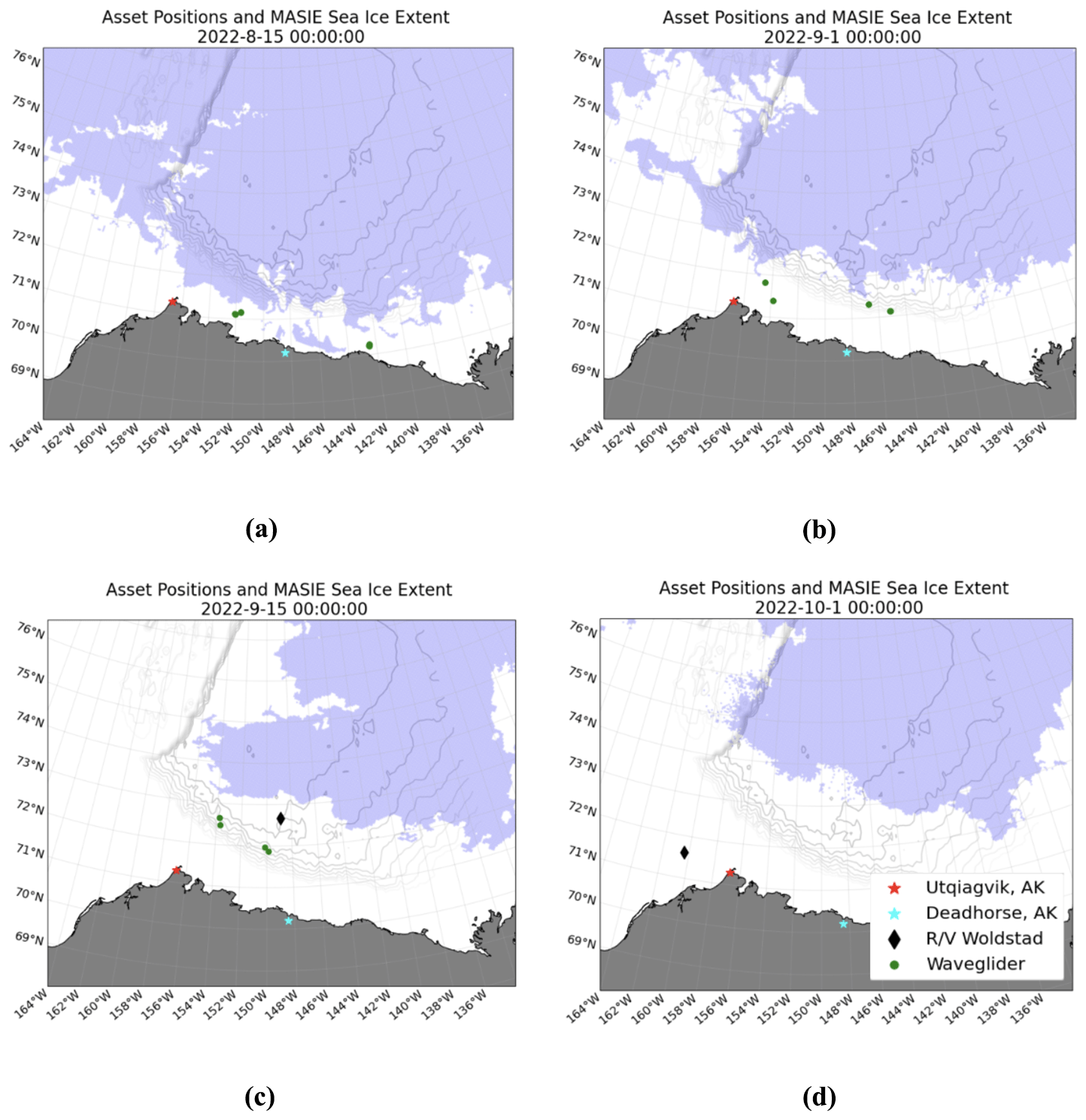
Figure 1Sea ice coverage, indicated by blue coloring, from the Multisensor Analyzed Sea Ice Extent – Northern Hemisphere (MASIE-NH) product (U.S. National Ice Center et al., 2010) for (a) 15 August, (b) 1 September, (c) 15 September, and (d) 1 October 2022. “Sea ice extent” refers to the area where the MASIE-NH product indicates greater than 0 % ice concentration. The positions of the research vessel (R/V) Woldstad (black diamond) and the Wave Gliders (green circle) on each date are shown. Bathymetry contours from 1000 to 6000 m (gray lines) from the ETOPO2 product (Smith and Sandwell v. 8.2: ° topography and bathymetry) are shown for reference.
Salinity controls stratification in the cold Arctic seas, enabling the uniquely polar phenomenon of colder, less dense, and fresher waters situated above warmer, denser, and saltier waters. Variations in upper-ocean salinity and the resulting stratification modulate the surface ventilation of stored subsurface heat, which can affect upper ocean temperature and thus sea ice formation and melt (e.g., Smith et al., 2018). During summer, melting sea ice leaves a layer of fresh, cold water at the ocean surface (Dewey et al., 2017). By mid-September, the sea ice extent reaches a minimum; the melting stops, and the ice edge begins to advance. The freshwater deposited by melting sea ice during its seasonal retreat may increase near-surface stratification, suppressing the upward mixing of heat from the warmer subsurface waters and thereby enhancing surface cooling, as shown by Crews et al. (2022). Increased stratification from melted sea ice may precondition the ocean for autumn sea ice formation, but there are very few in situ ocean and sea ice observations of this connection.
Salinity and Stratification at the Sea Ice Edge (SASSIE) is a NASA physical oceanography mission that aims to clarify the role of salinity and upper-ocean stratification in the Arctic Ocean. The primary goal of SASSIE is to better understand how the salinity anomalies generated by summer ice melt in the western Arctic evolve in space and time and ultimately how they affect the upper-ocean structure and the formation of sea ice in the early autumn. This paper describes data collected during the SASSIE field campaign that took place in August–October 2022 in the Beaufort Sea, including in situ measurements collected from a ship and a suite of uncrewed and drifting platforms, as well as remote sensing measurements collected from an aircraft. Satellite measurements (for instance, sea surface salinity, temperature, and height, surface winds, and sea ice concentration) are also a crucial part of the SASSIE mission data but are not addressed here.
1.2 Campaign overview
The SASSIE campaign focused on capturing three regimes in the Beaufort Sea, a region characterized by strong near-surface salinity stratification. Late-summer sea ice melt was sampled with a fleet of four Wave Gliders that traveled progressively northward from mid-August to early September as the sea ice retreated (Fig. 1a, b; Table 1). SASSIE's intensive observing period, from early September to early October, centered around the ship- and aircraft-based campaign during the transition between the summer melt season and autumn freeze-up (Fig. 1c, d). This main phase of the campaign focused on the region of the Beaufort Sea bounded by the shelf break to the south and the sea ice edge to the north between 154° W and 145° W (Fig. 2). Following the intensive ship- and airborne campaigns, the early part of the freeze-up was sampled with several floats and drifters that remained in the water after the ship departed.
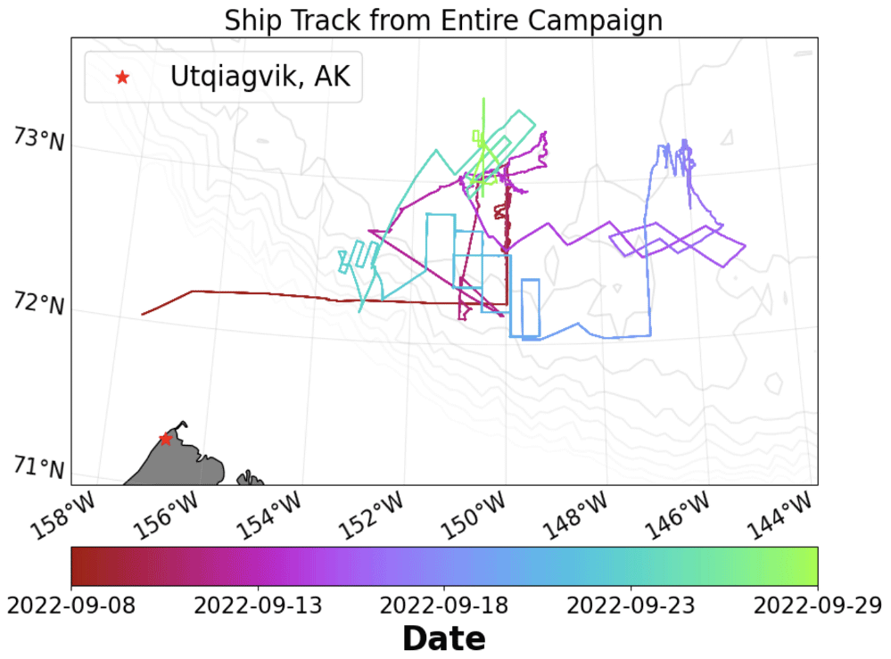
Figure 2The track of R/V Woldstad throughout the SASSIE campaign and colored by date. Bathymetry data (gray lines) from 1000 to 6000 m at an interval of 300 m are added for reference.
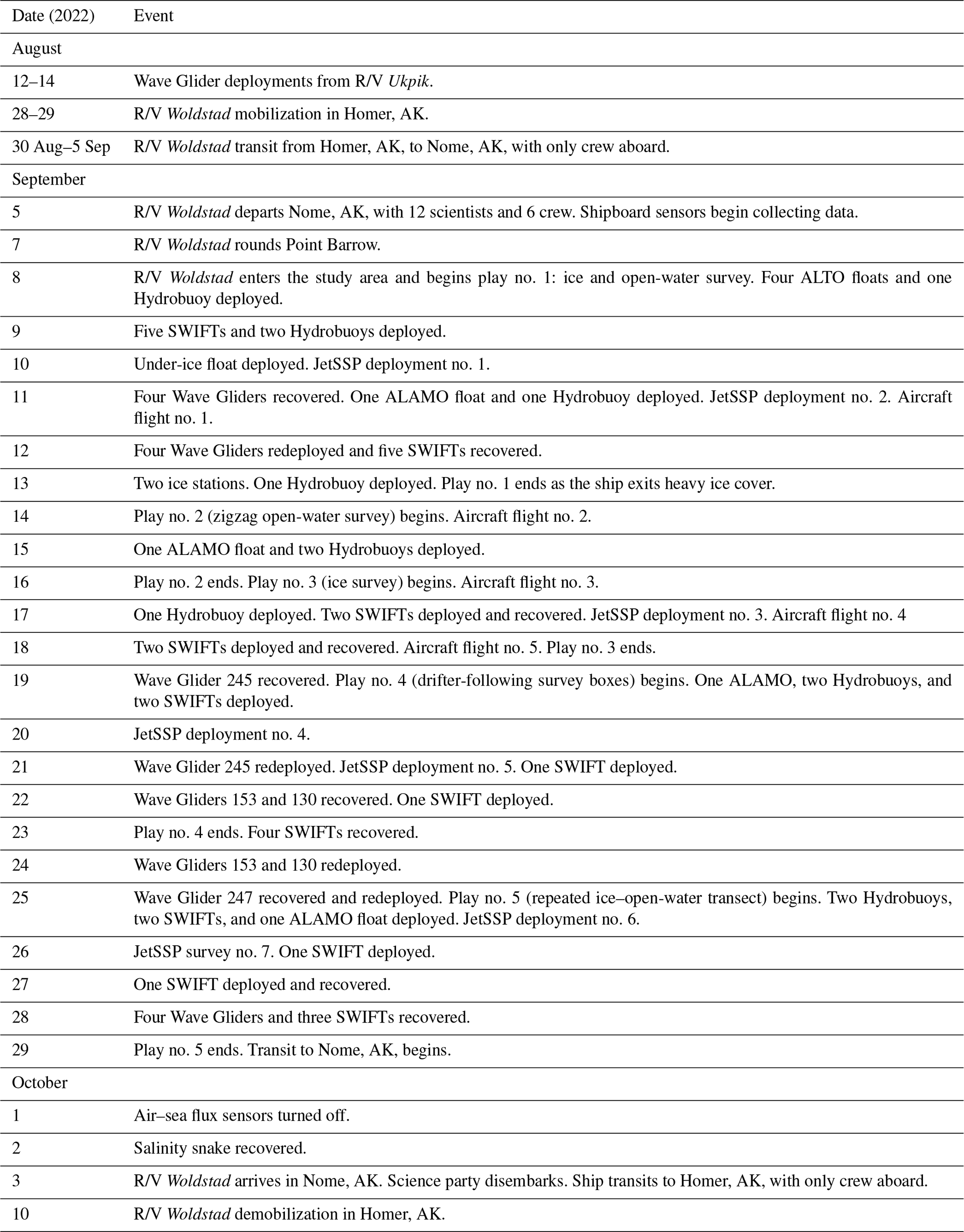
The major daily activities of the SASSIE campaign are summarized in Table 1. An animated depiction of the platforms is included in the Supplement.
Table 1A timeline of SASSIE events. Dates are given in local time. All other dates and times in this paper are in UTC. The Plays referred to in the table are described in Sect. 3. Note that SWIFT stands for Surface Wave Instrument Floats with Tracking, ALAMO stands for Air-Launched Autonomous Micro-Observer, and ALTO is a profiling float manufactured by Marine Robotic Vehicles.
A major objective of the SASSIE mission is to deliver quality-controlled data products to NASA's Physical Oceanography Distributed Active Archive Center (PO.DAAC) to foster broad utilization of the data within the broader scientific community. This paper outlines the campaign and describes the 15 SASSIE datasets archived at the PO.DAAC and available at https://podaac.jpl.nasa.gov/SASSIE (last access: 29 May 2024). Python notebooks to download, read, and visualize the data are available at the SASSIE's data visualization GitHub page (https://doi.org/10.5281/zenodo.8308513) (Westbrook, 2023). Section 2 describes the data and processing for each of the platforms deployed during SASSIE. Section 3 gives information about how SASSIE data can be accessed. Section 4 details the five “Plays” that distinguish different periods of the research cruise, and the Appendix gives definitions of the abbreviations used in this paper.
2.1 Research vessel and ship-deployed instruments
The ship-based sampling of the SASSIE program was carried out on research vessel (R/V) Woldstad (Fig. 3), a 121′ (37 m) deep-draft steel vessel operated by Support Vessels of Alaska Inc. This section describes all measurements collected from R/V Woldstad. A thermosalinograph (TSG) and S-band navigation radar are permanently installed on the vessel, while the SASSIE team supplied all other shipboard instruments.
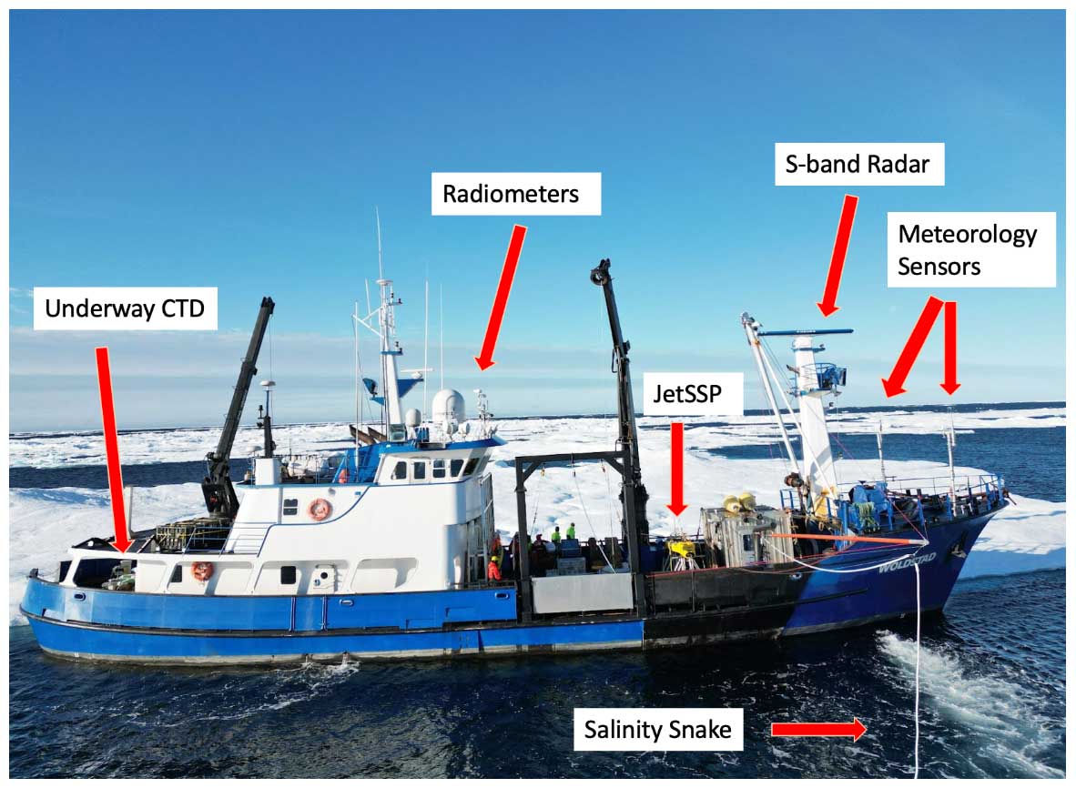
Figure 3R/V Woldstad. The photo was taken during the ice station on 13 September 2022. Note (1) the boom for the salinity snake protruding from the starboard side of the ship in the foreground, (2) two air–sea flux masts on the bow, (3) the radiometers above the bridge, (4) the JetSSP ready for deployment on the foredeck, (5) uCTD (underway conductivity–temperature–depth sensor) winch on the stern, and (6) S-band radar antenna on the mast.
2.1.1 Thermosalinograph (Drushka, 2023a)
The shipboard TSG system pumped water from an intake on the ship's hull at around 4 m depth through a Sea-Bird Electronics (SBE) 38 temperature sensor, a vortex debubbler, and finally a SBE 21 SeaCAT TSG. Temperature and conductivity data were logged every 10 s using Seasave software. Temperature measurements were made from both the SBE 21 and SBE 38 instruments; the SBE 21 temperature measurement is only used for the salinity computation. The SBE 38 temperature more accurately reflects the ocean temperature because the sensor measures seawater prior to it going through the TSG.
Temperature data were quality-controlled by removing values greater than 15 °C (<0.001 % of data) and spikes, which were defined as anomalies larger than 0.3 °C over 1 min (<0.005 % of data). Salinity data were quality-controlled by removing values smaller than 22 (<0.03 % of data) and negative spikes, which were defined as anomalies larger than −0.08 over 1 min (<0.5 % of data). Comparisons of salinity measurements from the TSG and from the three CTD (conductivity, temperature, and depth) sensors on the JetSSP (see Sect. 2.2.2), during periods when the upper ocean was well-mixed and all JetSSP sensors agreed, indicate that the ship's TSG had a −0.05 (fresh) bias. This bias was corrected in the final data product.
The large fluctuations observed in the temperature and salinity time series (Fig. 4) primarily reflect the spatial variability captured as the ship moved between open regions south of the ice edge and areas with low to moderate ice cover. Surface waters in the SASSIE domain were typically warmer and saltier in open water (1 to 2.5 °C, 26 to 28) and cooler and fresher within the ice (−1 to 0 °C, <26) (Fig. 5). An exception is the strong variability seen from 19–23 September, when the ship was in open water and sampled a region with strong fronts (Fig. 4).
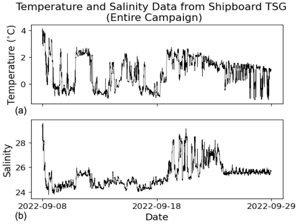
Figure 4Temperature (a) and salinity (b) records from the ship's thermosalinograph (TSG) during the SASSIE campaign.
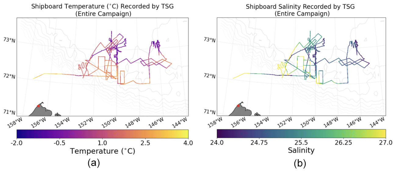
Figure 5(a) Temperature and (b) salinity from the shipboard TSG along the ship track from the entire SASSIE campaign.
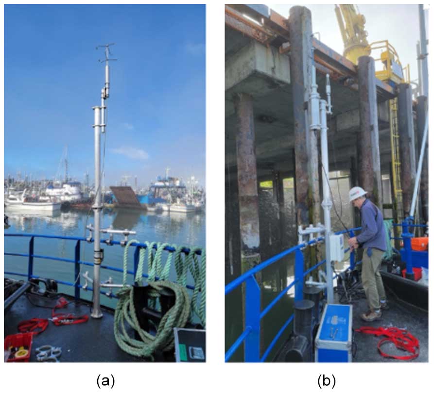
Figure 6(a) Starboard bow air–sea flux mast instrumented with Metek. (b) Port bow mast instrumented with the DCFS system and LI-COR.
2.1.2 Meteorology and air–sea fluxes (Menezes and Zippel, 2023)
Shipboard atmospheric measurements (wind speed and direction, shortwave and longwave radiation, barometric pressure, air humidity, and air temperature) were made almost continuously throughout the SASSIE cruise from two masts (on the port and starboard side of the bow, which were instrumented with the Woods Hole Oceanographic Institution (WHOI) DCFS (direct covariance flux system), Metek uSonic-3, and LI-COR 7500; Fig. 6) and from a barometer and radiometers mounted above the ship's wheelhouse (Table 2). These measurements are used to calculate air–sea heat and momentum fluxes using both the direct covariance method (Edson et al., 1998) and the traditional bulk flux algorithm from state variables. This dual strategy was chosen because the presence of sea ice modifies the surface roughness and surface temperature, making the efficacy of traditional bulk flux algorithms within 5 km of ice cover uncertain (Fairall and Markson, 1987).
Table 2Shipboard meteorological sensors deployed during SASSIE. Ship position and navigation data and sea surface temperature from the salinity snake were also used to compute bulk flux estimates.
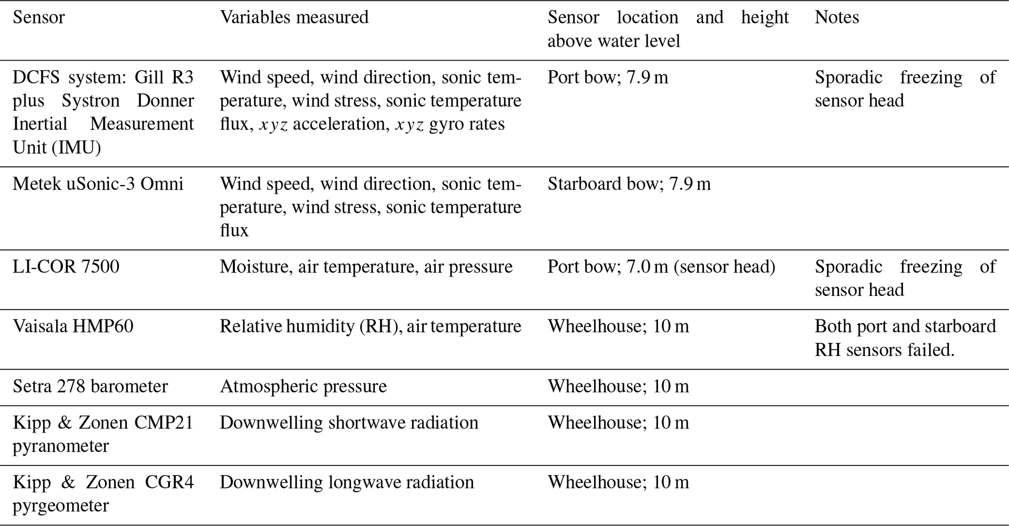
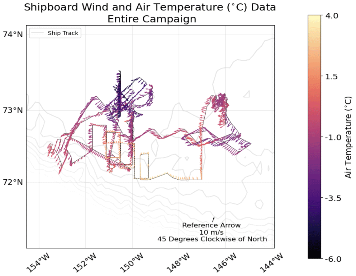
Figure 7Wind speed and direction measured from R/V Woldstad throughout the SASSIE campaign. The arrows are colored according to the air temperature. Bathymetry contours are shown for reference.
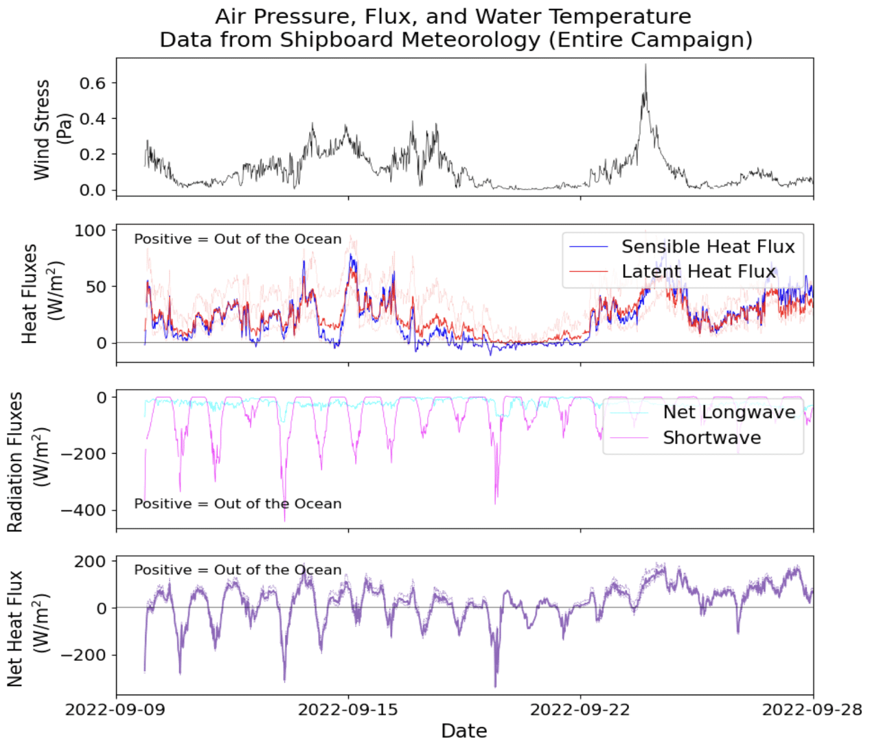
Figure 8Surface flux measurements measured from R/V Woldstad. (a) Wind stress (Pa). (b) Latent (red) and sensible (blue) heat flux (W m−2), with faintly colored lines showing uncertainty in the latent heat from RH values. (c) Net longwave (blue) and shortwave (pink) radiation (W m−2). (d) Net heat flux (solid line) and its uncertainty (faint lines).
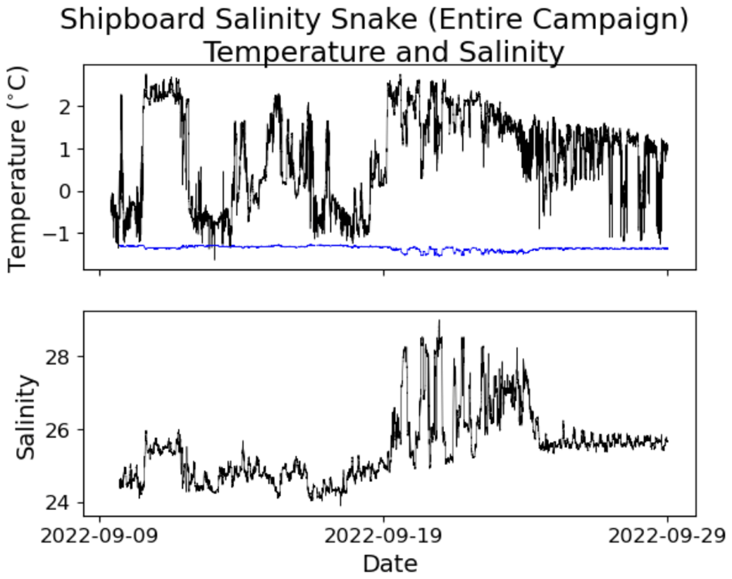
Figure 9Shipboard salinity snake temperature and salinity measurements throughout the entire SASSIE campaign. The blue line indicates the freezing temperature of the water.
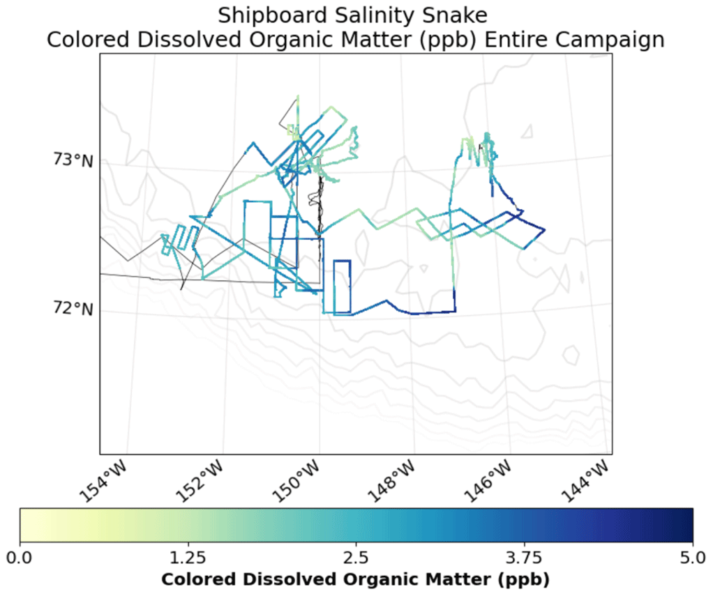
Figure 10Colored dissolved organic matter measurements from the shipboard salinity snake throughout the SASSIE campaign. Ship track (black line) and bathymetry contours from 1000 to 6000 m shown for reference.
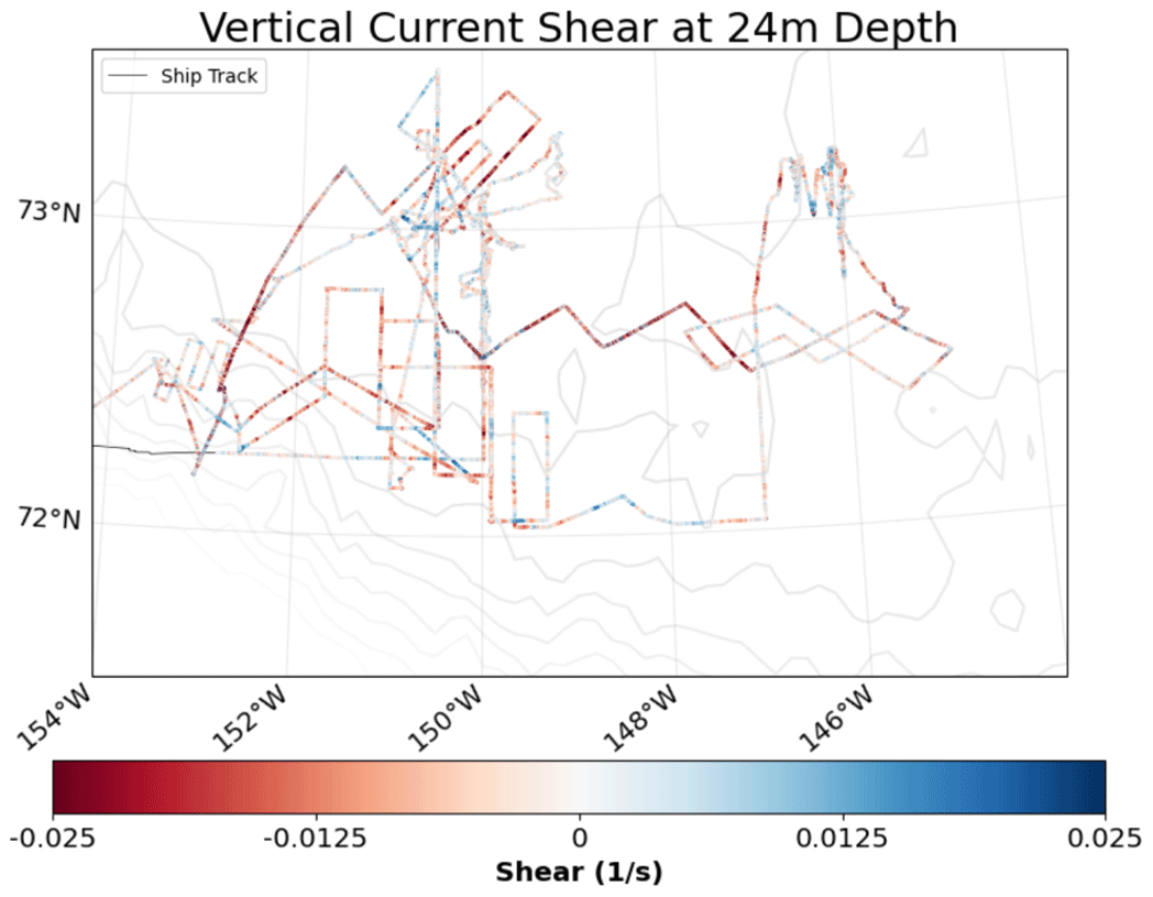
Figure 11A map of vertical current shear at 24 m depth collected by the ADCP on R/V Woldstad throughout the SASSIE campaign.
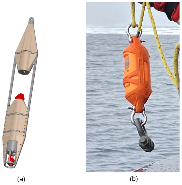
Figure 12(a) uCTD and (b) cCTD (CastAway conductivity–temperature–depth sensor) instruments. The uCTD has a total length of 1.08 m and the cCTD a total length of 0.20 m.
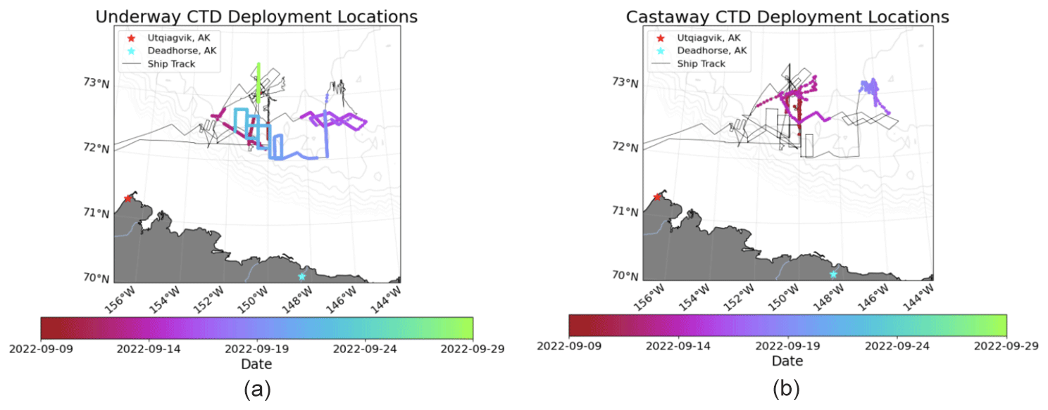
Figure 13Locations of (a) uCTD and (b) cCTD profiles colored by date, along with the ship track (black line). Individual casts are hard to distinguish as they are close together. Bathymetry data (gray lines) are added for reference.
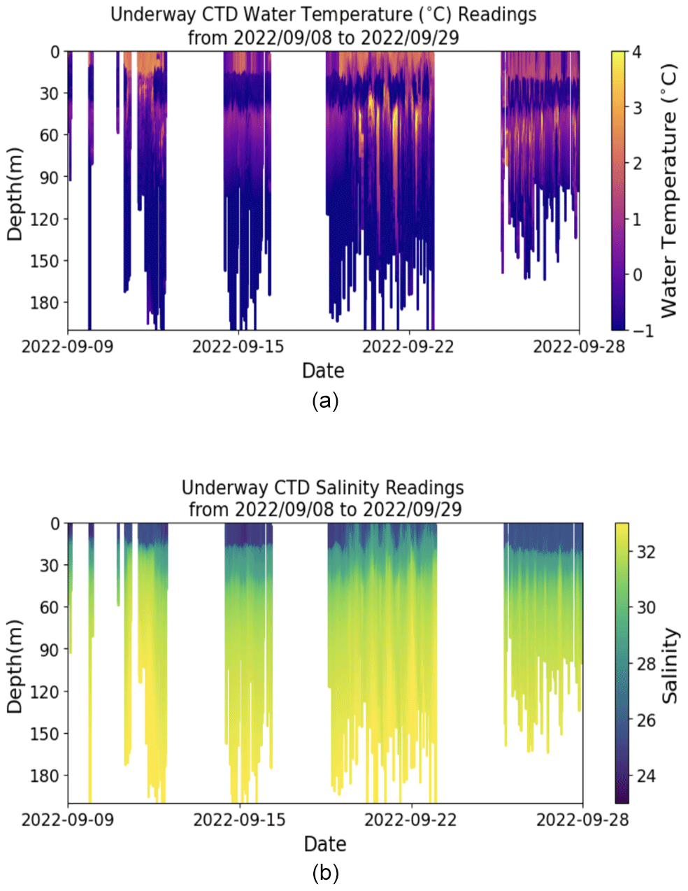
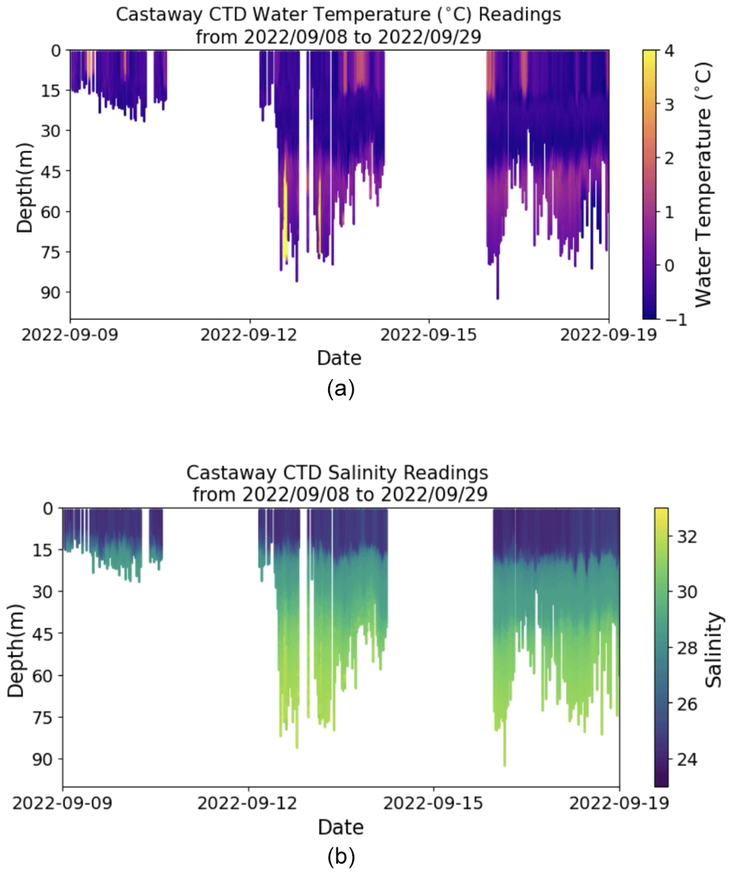
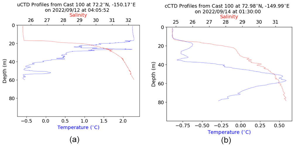
Figure 16(a) An example uCTD temperature (blue) and salinity (red) from 12 September at 05:40Z at 72.25° N, −150.5° E. (b) An example cCTD cast from 14 September at 01:30Z at 72.98° N, −149.99° E. Note the subsurface temperature maxima at ∼20 m and at ∼55 m in panel (b). The uCTD cast was taken in open water, whereas the cCTD cast was taken within the ice.
Detailed quality control processes for the meteorological measurements are as follows:
-
Wind speeds. Mean wind speeds between the two anemometers differed by as much as 10 % due to flow distortion around the ship's superstructure. The ship's flow distortion was found to be a strong function of apparent wind angle, with a large blockage caused from the forward radar mast (roughly +150° from the bow for the port side sensor and −150° from the bow for the starboard side sensor). A linear average of the two wind speeds would effectively distribute the bias evenly between the two sensors. A study using multiple wind sensors on a buoy showed a similar bias pattern with an apparent wind angle (Schlundt et al., 2020) and highlighted that the difference between the two sensors' wind speeds was distributed such that the upwind sensor accounted for roughly 75 % of the difference, and the downwind sensor accounted for roughly 25 % of the wind speed difference. We followed these percentages of Schlundt et al. (2020), reducing the upstream sensor by 75 % of the wind speed difference and increasing the downwind sensor by 25 % of the wind speed difference, with the error determined from the average percentage difference between the two wind sensors at relative direction from +100 to −100°. For directions where one sensor was obstructed by the radar mast (near °), this correction was not considered (since the nature of the flow distortion was different), and the unobstructed sensor data were used uncorrected. An ad hoc correction was applied to each mean wind estimate informed by previous ship and buoy computational fluid dynamics studies to reconcile the 10 % mean wind speed errors as a function of the ship's relative direction. True wind speeds and directions are then estimated by subtracting the ship's velocity vector (estimated from the navigation data). The two sonic anemometer time series are de-spiked and averaged to form a blended wind speed product.
-
Air temperature. The Vaisala data reported intermittently and had numerous spikes. The LI-COR temperature was recorded from a sensor in the instrument's electronics box, which was not radiation-shielded and so exhibited high bias under strong shortwave radiative forcing. Sonic temperature measured from anemometers is known to differ from the true temperature due to the sensitivity of the speed of sound in air to water vapor. In most cases, sonic temperature is subject to sensor drift to a variety of factors, including the temperature of the sensor itself. For this deployment, the Metek uSonic temperature was relatively stable due to the generally low absolute humidity in cold temperatures and because the sensor head was temperature controlled through a heating element. This lack of temperature drift was apparent through a high correlation between the nighttime LI-COR air temperature (when the LI-COR sensor was not subject to radiative heating) and the Metek uSonic temperature. Daytime air temperature values between the LI-COR and Metek were still correlated; however, they showed a bias, with the LI-COR temperatures larger than the Metek temperatures, consistent with radiative heating of the LI-COR sensor. A corrected temperature product was created by finding the constant offset between the Metek uSonic temperature and the nighttime LI-COR air temperatures values to replace the biased daytime LI-COR air temperature values. This corrected temperature product resulted in much better agreement between bulk and direct buoyancy fluxes than if any of the three raw air temperatures were used uncorrected. Figure 7 shows wind speed and direction measurements colored by air temperature.
-
Direct momentum fluxes. Direct covariance estimates of the wind stress are made following the Edson et al. (1998) method. Raw wind speed data are corrected using the acceleration/gyro system to remove the contamination from ship pitch, heave, and tilt motions.
-
Inertial dissipation fluxes. Estimates of total kinetic energy (TKE) dissipation rate are made by fitting a theoretical model to the measured power spectra of vertical velocity from the sonic anemometers. A TKE balance is assumed and inverted for wind stress, as described in Fairall et al. (1990) and Edson et al. (1991).
-
Bulk fluxes. Bulk fluxes are estimated from the COARE (Coupled Ocean–Atmosphere Response Experiment) 3.5 algorithm (Edson et al., 2013) using blended wind speed, air temperature products, radiometer measurements, and sea surface temperature (SST) (see Sect. 2.1.1). Due to the failure of the Vaisala RH sensors and the noise of the LI-COR 7500, bulk fluxes are run with a constant RH (RH = 89) informed by previous cruises (Persson et al., 2018). Errors in the latent heat flux are reported as the range of fluxes estimated from the range of RH values reported in Persson et al. (2018) (RH = 70 to RH = 100). Figure 8 provides a summary of surface flux measurements throughout the campaign.
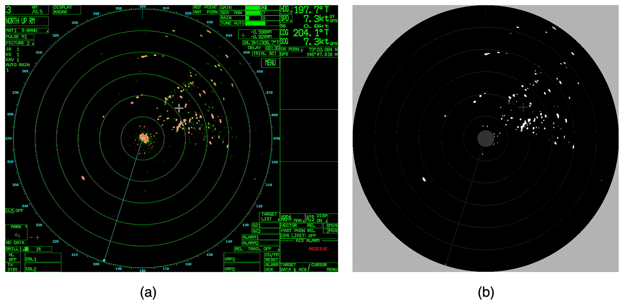
Figure 17(a) S-band radar snapshot on 19 September 2022 at 00:34Z as the ship was transiting southward out of the ice. Metadata are shown in the image; total range is 3 nmi (5.6 km), with 0.5 nmi (0.9 km) per range ring (upper left of the image). The image is oriented such that up corresponds to north. The ship's heading is shown as the cyan line on the image and the text in the upper-right corner. The presence of ice is indicated by the red–yellow patches in the upper-right quadrant of the range rings. The bright area in the center of the image is sea clutter. (b) The classified image corresponding to panel (a), in which each pixel has been classified as sea ice (white), not sea ice (black), sea clutter (dark gray), or no data (light gray).
Winds in the SASSIE domain were predominantly easterly (Fig. 7). SASSIE captured three periods of relatively strong winds (∼14–15 September, 17–18 September, and 24 September) that drove turbulent cooling and a period of very weak winds (19–20 September) during which sensible and latent fluxes were near zero. Throughout the campaign, downwelling radiation remained fairly consistent. As the daily peak in solar radiation decreased during the transition to autumn, net heat flux transitioned from predominantly warming the ocean in early September to cooling the ocean starting at around 22 September (Fig. 8).
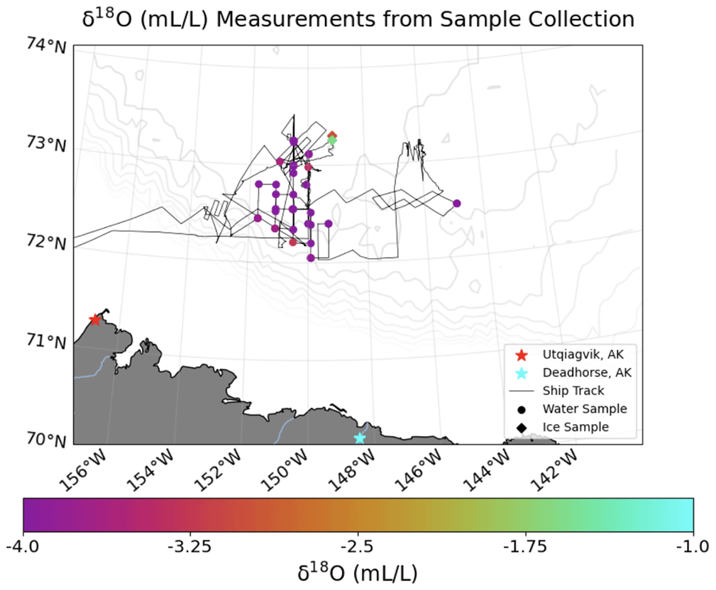
Figure 18Locations and measurements of the δ18O ratio measurements and the value recorded. Water samples are shown as circles, and ice samples are shown as diamonds. The track of R/V Woldstad is shown as a black line.
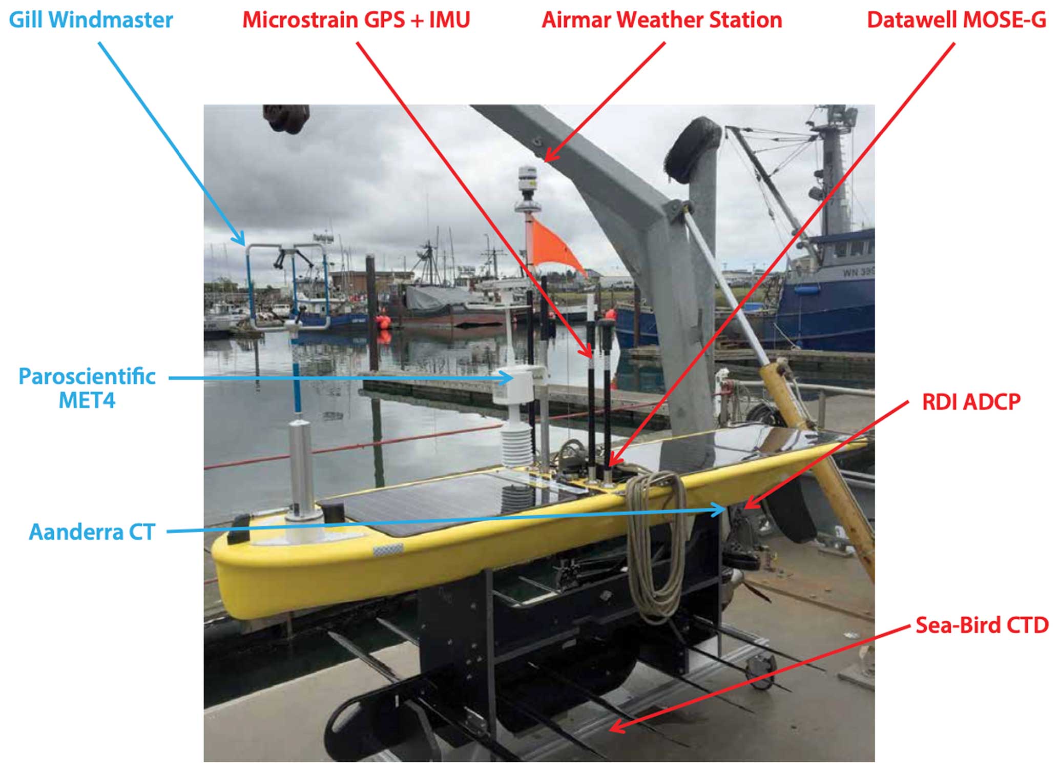
Figure 19Labeled photo (Thomson and Girton, 2017) showing the instruments on Wave Glider SV3-153.
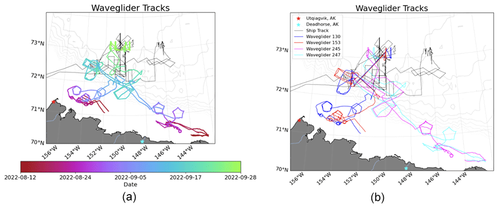
Figure 20Paths of the four Wave Gliders throughout the course of the SASSIE campaign colored by (a) time and (b) Wave Glider number. The track of R/V Woldstad (black line) and bathymetry contours (gray lines) are also shown for reference.
2.1.3 Salinity snake and FDOM/CDOM (Schanze, 2023)
To measure the very near-surface salinity without contamination from the ship's wake, a salinity snake (Ho and Schanze, 2020) was deployed on R/V Woldstad during SASSIE. The salinity snake instrument consists of four main components: a boom, an intake hose, a pump, and a shipboard apparatus. A boom with a halyard is deployed to the starboard side of the vessel, which is used to position a flexible steel-reinforced rubber hose outside the wake of the ship. Water is pumped from the surface of the ocean at approximately 0.05 m depth, passes through a de-bubbler system, and enters a Sea-Bird SBE 45 TSG (note that this is completely independent from the TSG that is permanently installed on R/V Woldstad). Water then passes through a Turner Designs C-FLUOR fluorometer with RS232 output. The fluorometer yields measurements of fluorescent dissolved organic matter (FDOM), which is a proxy measurement of colored dissolved organic matter (CDOM). The FDOM probe is factory-calibrated and needs no further calibration. A SBE 56 temperature logger inside the seawater end of the intake hose makes a continuous measurement of water temperature at ∼0.05 m depth.
Ancillary data generated by the salinity snake system include the flow rate, pump suction, and instrument pressure. These values are used in the quality control of the salinity data to ensure that a flow rate between 0.5–3 L min−1 was present at the instrument.
The salinity snake collected data throughout the SASSIE cruise (Fig. 9) and captured the same general temperature and salinity patterns as the shipboard TSG (Fig. 4b). FDOM patterns (Fig. 10) are distinct from those of temperature or salinity.
2.1.4 ADCP (Gaube, 2023)
A hull-mounted 300 kHz Teledyne Workhorse Mariner ADCP (acoustic Doppler current profiler) was used to estimate vector current profiles from ∼5 to ∼70–120 m depth, depending on the concentration of scattering material in the water. The ADCP was operated in narrowband mode and ADCP measurements were logged using VmDas software every 1 min. Unfortunately, the ship's heading sensor was not functioning correctly, and so the heading could not be removed from the current vectors; thus, vector ocean velocity estimates could not be made. Vertical current shear magnitude was estimated as the vertical derivative of current speed without any heading corrections and is archived in the data collection. The vertical gradient was computed on a vertical grid located at the midpoints of ADCP bins; currents larger than 2 m s−1 were flagged as errors and removed from the data prior to computing the vertical gradient. Figure 11 illustrates the patterns of vertical shear in the upper ocean. The largest values generally correspond to periods with stronger winds (e.g., Fig. 7). Areas of alternating positive and negative shear were also observed, for instance, south of 73° N from 152° W to 149° W, consistent with the strong sub-mesoscale fronts observed in the upper-ocean temperature and salinity data (play no. 4; see Sect. 4.4).
2.1.5 uCTD and cCTD measurements (Schmidgall, 2023; Pérez Valentín, 2023)
The underway CTD (uCTD; Fig. 12a) system was used to measure vertical profiles of temperature and conductivity (and thus salinity and density) at survey speed throughout the SASSIE experiment. The uCTD, a platform that was developed and built at APL-UW (University of Washington Applied Physics Laboratory), was primarily deployed in open water, whereas in areas with sea ice, a SonTek CastAway CTD (cCTD; Fig. 12b) was more typically used. A total of 2518 CTD casts were collected in the Beaufort Sea (Fig. 12), 2246 of which were made with the uCTD.
The uCTD consists of an armored and faired RBR concerto CTD sensor (RBR, Ottawa, Canada) that was lowered and raised using an electric fishing reel, which was mounted to a stand at the aft starboard side of R/V Woldstad. The line was extended several meters to the aft starboard side with a boom to sample away from the ship's prop wash. Nonetheless, it must be assumed that the upper ∼4 m of the ocean behind the ship were well mixed; those data must be used with caution. The RBR concerto recorded measurements of conductivity, temperature, and pressure at 32 Hz. The average fall rate of the sensor was 2.1 m s−1, giving a vertical sampling interval of ∼6.5 cm. The horizontal spacing between continuous casts averaged ∼0.8 km, and the average depth of the casts was 100 m, with some casts reaching 200 m.
The uCTD data were offloaded via the RBR Ruskin software, quality-controlled, and gridded onto a uniform vertical grid with spacing of 0.1 m. Only the data from the downcasts and deeper than 1 m are retained for analysis. The uCTD data were co-located with data from the shipboard navigation system to provide position information for each cast. The uCTD was deployed continuously (in “tow-yo” mode) as the ship steamed at 1–4 m s−1 whenever conditions permitted, which was typically in areas with sufficiently low ice cover that the ship could maneuver between floes. In slightly heavier ice cover (10 %–30 % sea ice concentration), when continuous profiling was not safe, the ship typically stopped every 30 min, and a single uCTD cast was collected. During rough seas (wind speeds greater than around 10 m s−1), the uCTD could not be deployed.
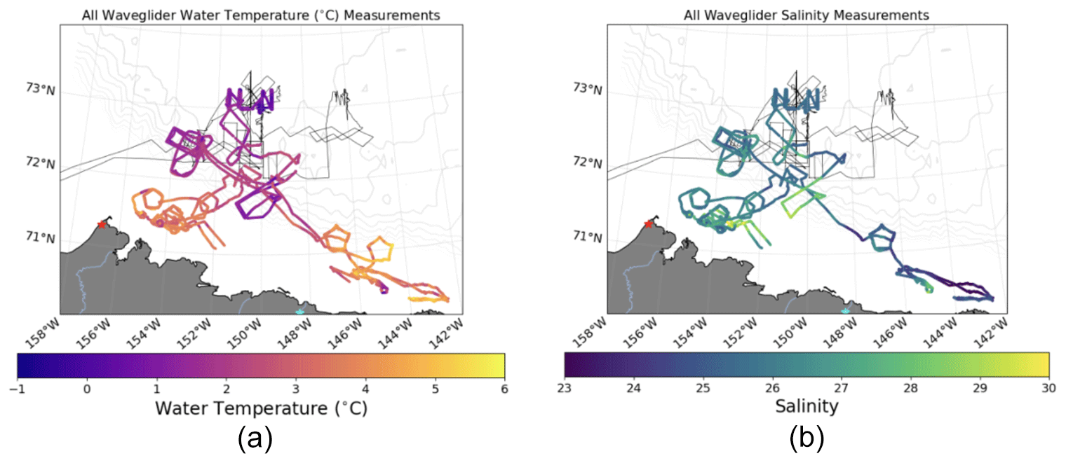
Figure 21Paths of all four Wave Gliders throughout the course of the SASSIE campaign colored by (a) water temperature and (b) salinity at 0.25 m depth, except in the case of salinity measurements of Wave Glider 153, which were taken at 1 m depth. The track of R/V Woldstad (black line) and bathymetry contours (gray lines) are also shown for reference.
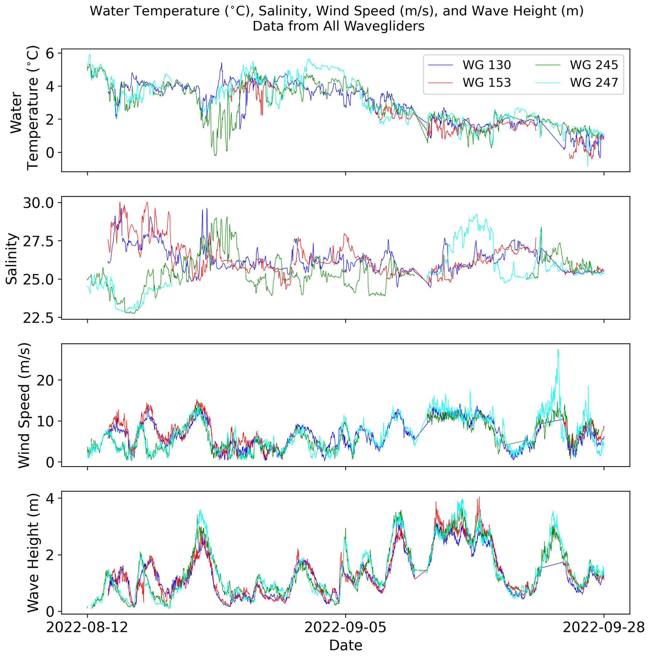
Figure 22Time series of water temperature, salinity, wind speed, and wave height measurements made by the four Wave Gliders throughout the SASSIE campaign. Temperature and salinity measurements are from 0.25 m depth, except for the salinity measurements from Wave Glider 153 that were made at 1 m depth.
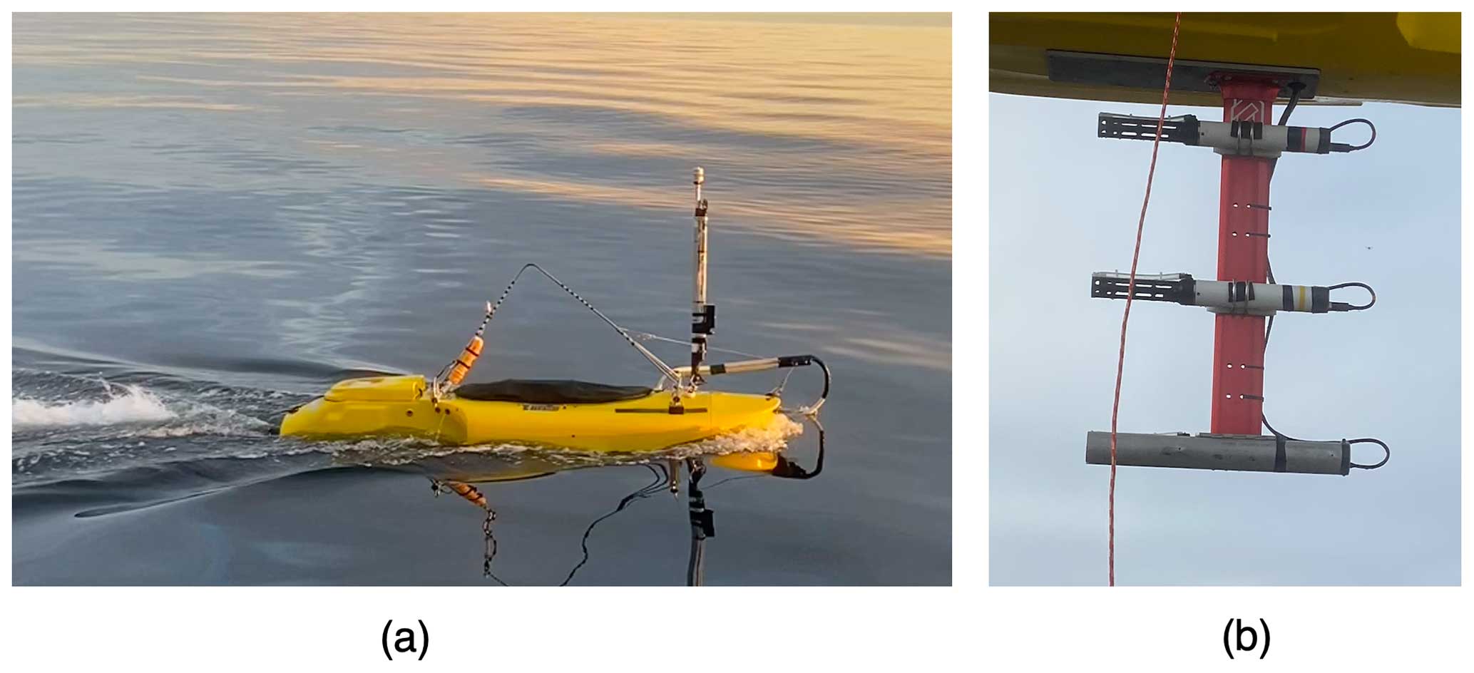
Figure 23(a) The JetSSP just after deployment. Note the forward meteorology mast and the hose off the port side for the salinity snake. (b) The 1 m long keel of the JetSSP with three CTDs; the front end of the platform is to the left in the photo. Photo credit: Alex de Klerk.
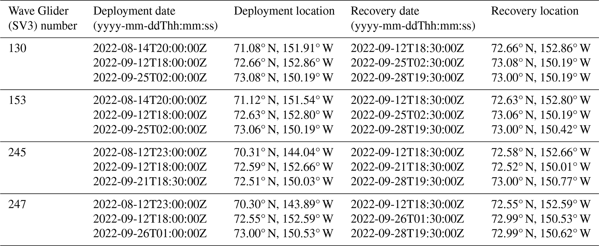
Table 3Deployments of Wave Gliders throughout the SASSIE campaign.
In cases where the uCTD could not be used, profiles were instead collected with the cCTD – typically every 30 min as the ship was underway. A total of 272 total cCTD casts were collected (Fig. 13b). The cCTD is a small, rugged, and technically advanced CTD designed for profiling to depths of up to 100 m (Fig. 12b). It records temperature, conductivity, and pressure at 5 Hz (resulting in ∼0.3 m vertical resolution), as well as GPS position information for each cast. Casts reached an average depth of 45 m, with considerable variance, depending on the ship's speed and amount of line used (Figs. 14, 15). The accuracy of the cCTD salinity measurements is roughly 0.1. Surface data from the cCTD were compared to TSG measurements to assess the accuracy of the cCTD measurements at the surface; profiles for which the cCTD temperatures were more than ±2 °C or the cCTD salinities were more than ±1.5 different from the nearest TSG measurements were discarded.
The uCTD and cCTD measurements collected during SASSIE reveal a wealth of horizontal and vertical upper-ocean structures (Figs. 14, 15, 16), including signatures of Pacific summer water (temperature maxima around 50 m depth), near-surface temperature maxima typical of the region (Jackson et al., 2010), and strong lateral salinity gradients in the upper 20 m.
2.1.6 S-band radar (Drushka, 2023b, c)
R/V Woldstad is equipped with a Furuno FAR2137SBB S-band marine navigation radar. The ship relied heavily on this radar for navigating through sea ice, particularly during the night and when visibility was low due to fog. X-band radar data have been used in ship-based studies of sea ice (e.g., Lund et al., 2018); S-band radar data have also been used for this purpose (Haykin et al., 1985).
During the SASSIE cruise, screenshots of the ship's S-band radar data were collected by splitting the signal and turning it into a video feed using a screen capture device (Epiphan AV.io HD; Fig. 17). This video feed was acquired using a command line video conversion program called “ffmpeg”, which saved screenshots (as jpeg files) at a specified time interval, typically every 60 s while the ship was in and around the ice. During JetSSP deployments in the ice, images were acquired every 10 s to map the ice evolution in higher resolution. While the ship was in open water for longer than 1 d, S-band acquisition was paused.
The S-band radar was actively used by the ship's captain and crew for navigation, and the radar settings were adjusted frequently, leading to inconsistencies in the data. Typically, the ship set the radar range to 6 to 12 nmi (11 to 22 km) during the daytime and 0.75 to 3 nmi (1.4 to 6 km) during the night or in heavy ice concentrations. The captain and first mate adjusted the range, heading orientation, and gain as needed to reduce clutter and identify safe routes through the ice. During the night, the radar was set to a lower-brightness night mode. The radar was switched to standby mode when personnel were on top of the pilot house.
Metadata were extracted from the images using MATLAB's computer vision toolbox. The pixels outside of the largest range ring were stripped from each image, and pixels within the range rings were georectified and stored as GeoTIFF images. A data product in which each pixel was classified as sea ice, not sea ice, sea clutter, or not data (e.g., range rings) was also developed (Drushka, 2023c). Pixels were classified based on their red, green, and blue (RGB) values. RGB values consistent with yellow to red color ranges were classified as “sea ice”, and those consistent with blue–green colors were classified as “no data”. RGB values were summed as a function of distance from the center of each image; sea clutter appears as a peak in this value. An iterative method was used to identify the distance from the center at which sea clutter could no longer be detected; pixels at smaller distances from center were flagged as clutter. The classified image corresponding to Fig. 17a is shown in Fig. 17b. Though the classification is imperfect, it is evident that these data reveal qualitative information about the presence of sea ice around the ship.
2.1.7 Bottle samples for δ18O (Drushka, 2023d)
Water samples were collected periodically throughout the cruise for δ18O isotope analysis to help differentiate the sources of the freshwater signals in the SASSIE domain – presumed to be a combination of sea ice meltwater, meteoric water (likely from the Mackenzie River), and Pacific seawater. A total of 45 water samples were collected, including two duplicates (Fig. 18). Water samples were collected from a Go-Flo bottle lowered from a line over the side of the ship to approximately 1 m (N=7 samples), 5 m (N=12), or 30 m (N=1) depth. An RBRduet temperature–pressure logger was attached to the Go-Flo bottle, providing accurate measurements of the depth and water temperature of the sample. An additional 21 water samples were collected from the salinity snake, which pumped water from ∼0.05 m depth. Finally, samples were collected during two ice stations on 13 September. Tailings from drilling into the sea ice were collected, melted, and stored in sample bottles.
All samples were stored in 20 mL glass scintillation bottles, sealed with Parafilm, and later analyzed using a mass spectrometer for δ18O isotopes at the Oregon State University Stable Isotope Laboratory.
Table 4List of sensors and variables collected by Wave Gliders.
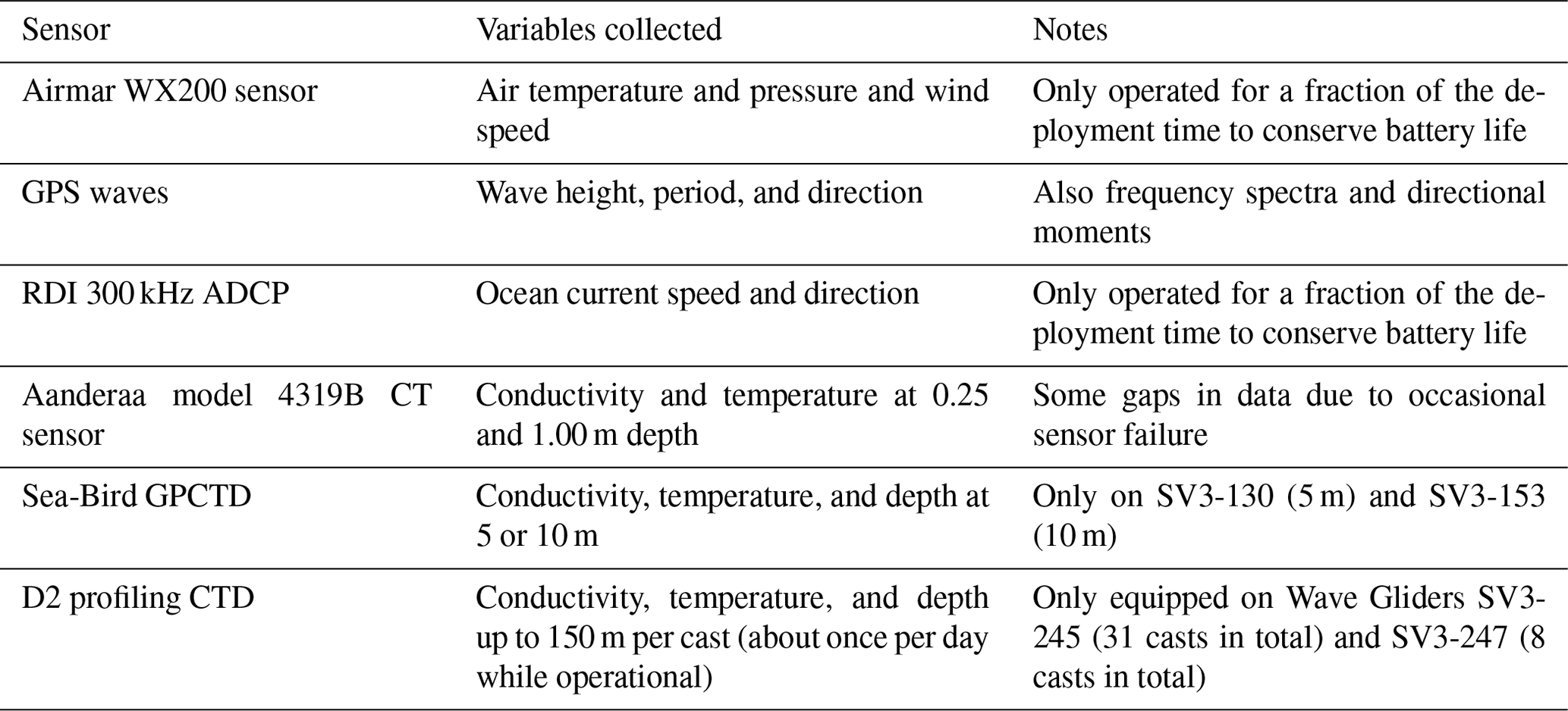
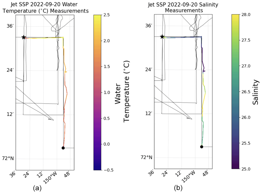
Figure 24Tracks of JetSSP deployment 4 on 20 September 2022 color-coded by (a) temperature and (b) salinity taken at 0.05 m depth. The thin lines show the track of R/V Woldstad. The black circle marks initial deployment location, and the black star marks the recovery.
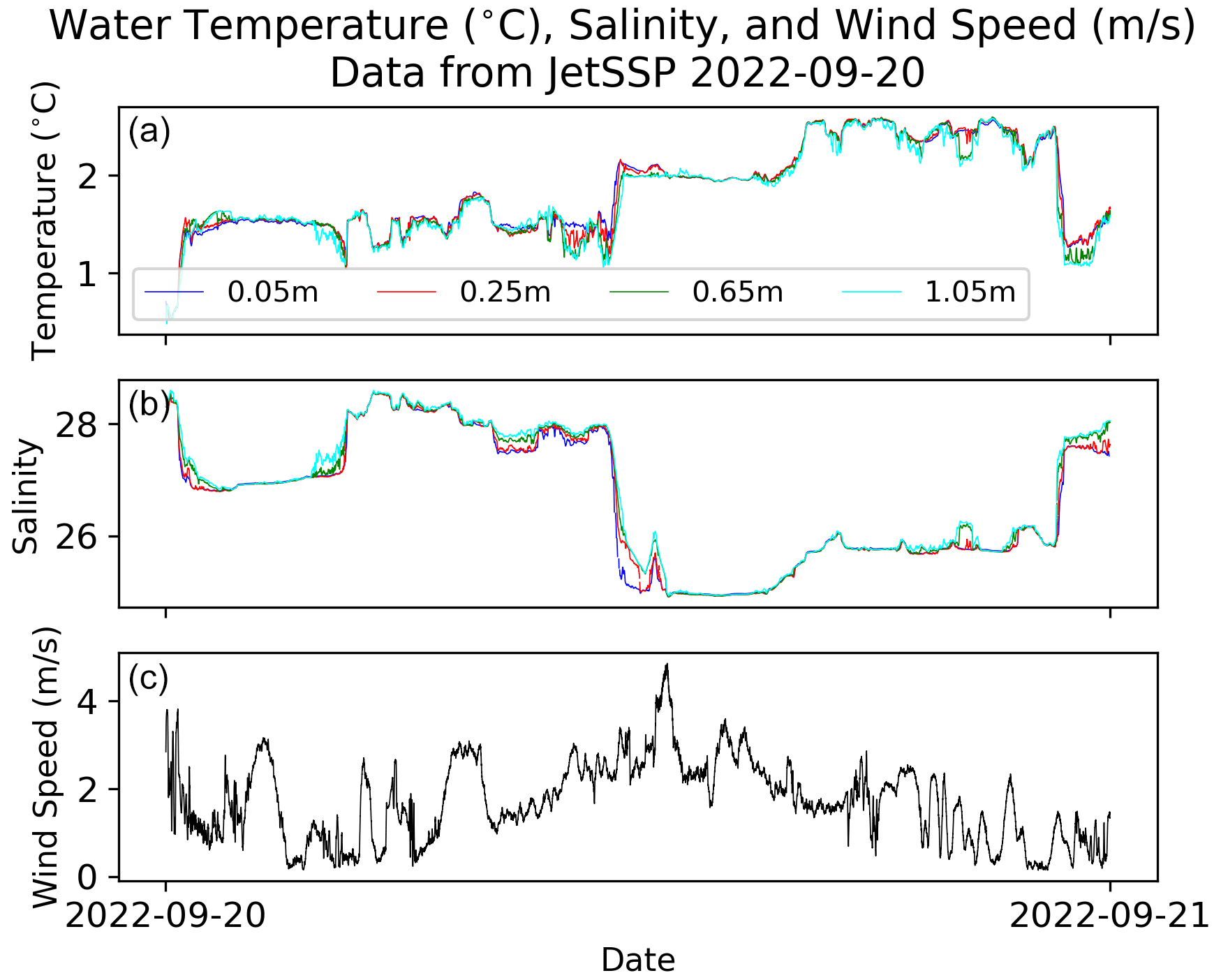
Figure 25(a) Seawater temperature, (b) salinity, and (c) wind speed records from JetSSP deployment on 20 September.
Salinity measurements are needed to interpret δ18O data, and salinity estimates collocated with each water sample are included in the δ18O dataset. Each sample made with the lowered Go-Flo bottle was collected within 5 min of a uCTD cast at the same location. Water samples made with the salinity snake were collocated with salinity snake data. The salinity of the sea ice samples estimated as a function of sea ice thickness (measured when the ice samples were made) based on Cox and Weeks (1974).
δ18O values of −5 to −2 mL L−1 were observed throughout the SASSIE domain, except for higher values (−2 to −1.5 mL L−1) in the sea ice samples (Fig. 18). While these values are generally consistent with previously observed δ18O values observed in Beaufort Sea upper-halocline water and sea ice meltwater, and significantly higher than δ18O values of meteoric water (e.g., Lansard et al., 2012), further analysis is needed to quantify the sources of freshwater in the area.
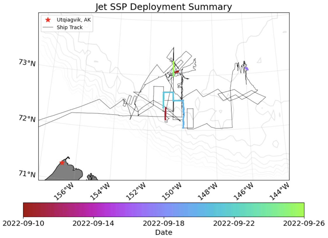
Figure 26Paths of JetSSP deployments throughout the course of the SASSIE campaign colored by time. The track of R/V Woldstad (black line) and bathymetry contours (gray lines) are also shown for reference.
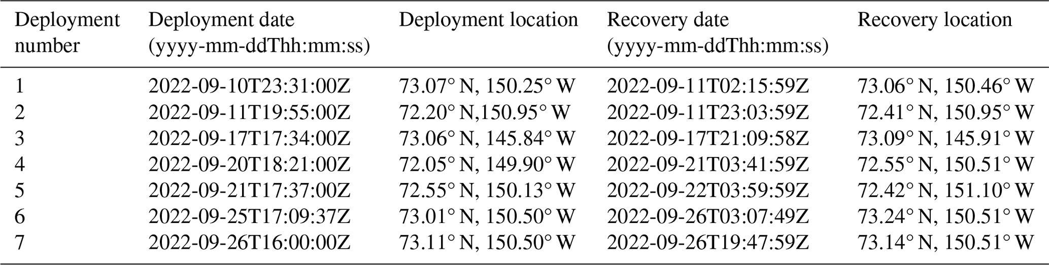
Table 5Deployment and recovery dates and locations for the JetSSP.
2.2 Piloted and drifting platforms
2.2.1 Wave Gliders (Thomson, 2023a)
Four Wave Gliders (model SV3 built by Liquid Robotics, Inc.) from APL-UW were operated throughout the SASSIE campaign. The Wave Gliders were deployed from R/V Ukpik operating out of Prudhoe Bay in early August. They were recovered for battery charging and redeployed twice from R/V Woldstad in September (Table 3), and the final recovery was in late September from R/V Woldstad. Each Wave Glider operated for approximately 50 d and covered almost 1000 nmi (1852 km), often within 10 nmi (20 km) of the sea ice (as determined from the National Weather Service (NWS) Alaska Sea Ice Program accessed at https://www.weather.gov/afc/ice, last access: 29 May 2024, an operational product that ingests visible imagery to help include low ice concentration areas).
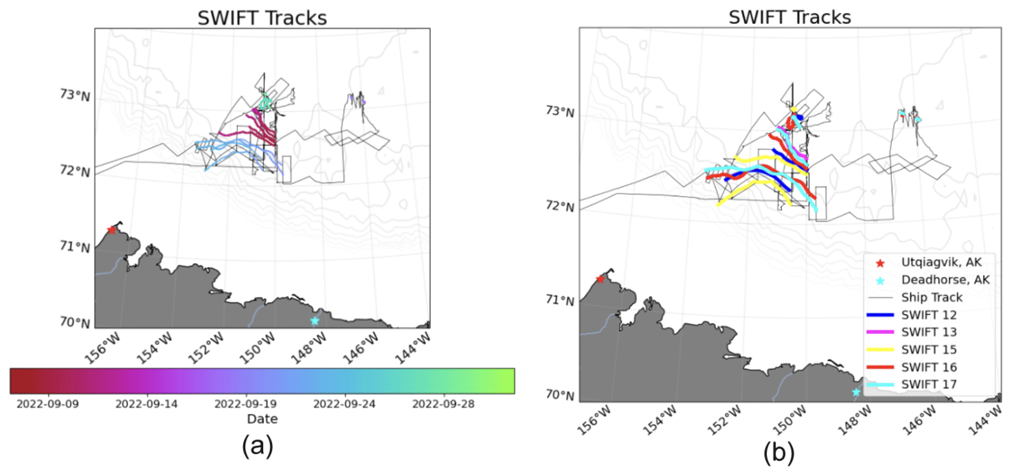
Figure 27Paths of the five SWIFTs over multiple deployments throughout the course of the SASSIE campaign colored by time (a) and SWIFT number (b). The track of R/V Woldstad (black line) and bathymetry contours (gray lines) are also shown for reference.
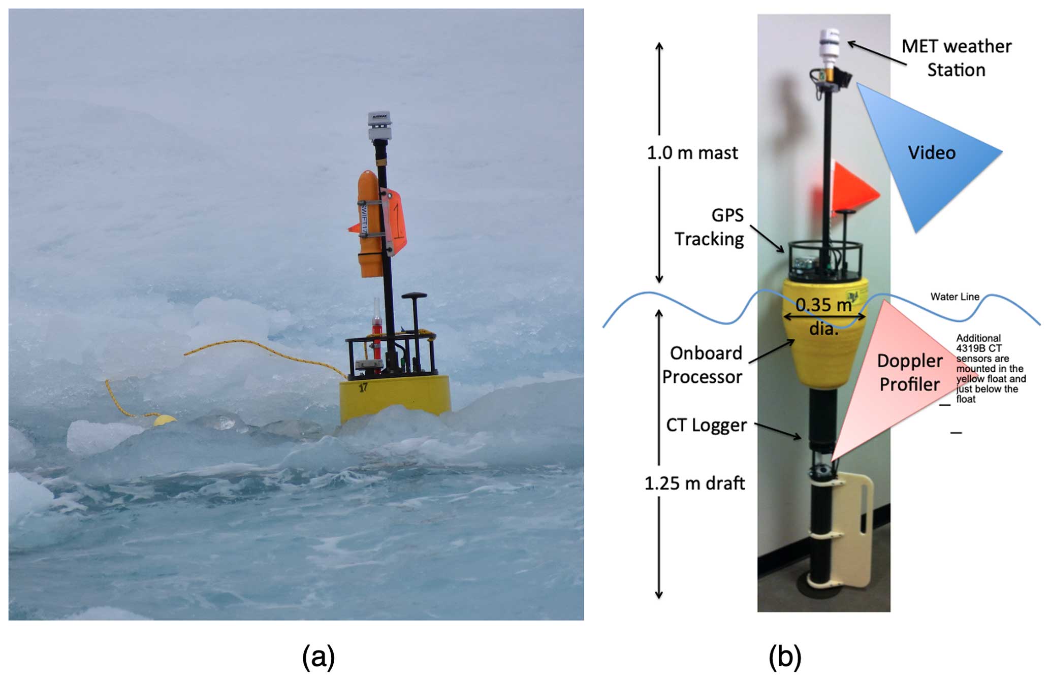
Figure 28(a) A SWIFT floating within slushy ice. Photo credit: Edwin J. Rainville. (b) A SWIFT in the lab with dimensions and notation. Visible in panel (a) is a small yellow float and the line that trails behind the drifting SWIFT to make it easier to recover with a grappling hook.
Each Wave Glider included a standard package to measure meteorological data (Airmar WX200 sensor), waves (GPS waves by Thomson et al., 2018), ocean currents (RDI 300 kHz ADCP), near-surface temperature and salinity (Aanderaa CT), and sub-surface temperature and salinity (Sea-Bird GPCTD) (Table 4). Some of these sensors, such as the ADCP and the Airmar, only operated for a fraction of the mission as a battery-saving strategy. Salinity measurements from the Aanderaa CT and the Sea-Bird GPCTD sensors agree with a root mean square difference of 0.1 (not shown). Two of the Wave Gliders include profiling winches for CTD measurements beneath the subsurface portion of the vehicles (8 to 150 m). These prototype systems collected a total of 39 profiles before failing; those data are included in the L1 data but did not pass quality control for inclusion in the L2 data.
2.2.2 JetSSP (Drushka, 2023e)
The JetSSP is an autonomous unpiloted surface vessel designed to measure salinity gradients in the upper meter of the ocean. The system consists of a 3.1 m long gasoline-powered jet kayak that is controlled using an onboard suite of drone hardware to enable autonomous navigation (Fig. 23). Telemetry data are broadcast over a 900 MHz antenna, as well as an independent Automatic Identification System (AIS) and Iridium trackers. The vehicle has fuel capacity to perform 12+ h autonomous sampling missions traveling at speeds of 4 to 5 kn. A 1 m long keel is bolted to the underside of the vehicle and outfitted with three SBE 49 CTDs that sampled below the water line (Fig. 23b).
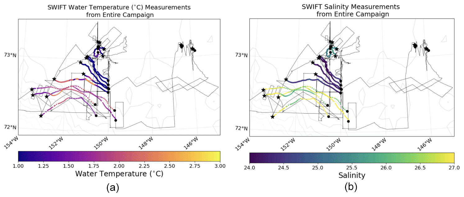
Figure 29(a) Temperature and (b) salinity measurements taken by SWIFTs throughout the SASSIE campaign. The track of R/V Woldstad (black lines) and bathymetry data (gray lines) are shown for reference. Deployment locations are shown as a circle, and recovery locations are shown as a star.
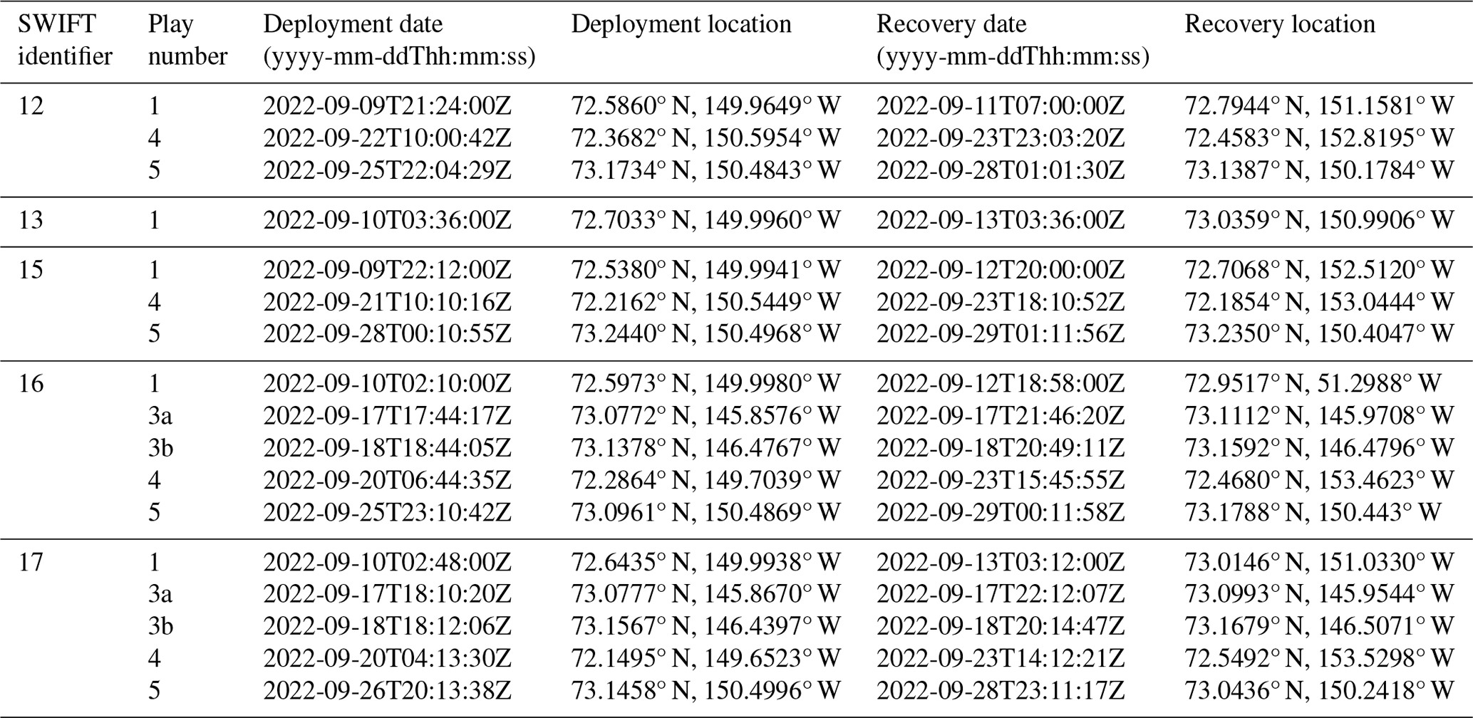
Table 6A list of deployment dates and locations for SWIFT buoys.
In addition, a miniaturized salinity snake consisting of a SBE 45 TSG, a positive displacement pump, and a vortex debubbler is mounted internally in order to sample water from a hose dragged on the surface. Using these four instruments, JetSSP is able to continuously measure salinity and temperature at nominal depths of 0.05, 0.25, 0.65, and 1.05 m, capturing the very near-surface signature of horizontal and vertical salinity and temperature gradients associated with freshwater layers (Figs. 24 and 25). A forward mast with an Airmar 200WX-IPX7 weather station reports air temperature and pressure and GPS-corrected true wind speed and direction. Data are logged at 6 Hz with a WET Labs DH4 logger.
The JetSSP platform was deployed from the ship and successfully collected data seven times (Table 5; Fig. 26). On the eighth deployment, the platform was lost.
2.2.3 SWIFT (Thomson, 2023b)
Five Surface Wave Instrument Floats with Tracking (SWIFTs; Thomson, 2012) were repeatedly deployed and recovered in the Beaufort Sea during the SASSIE field campaign (Fig. 27). SWIFTs are freely drifting buoys that measure waves, winds, temperature, salinity, turbulence, and velocity profiles in a surface-following reference frame (Fig. 28).
For SASSIE, additional conductivity and temperature (CT) sensors (Aanderaa model 4319B) were added to most buoys (Fig. 29b). The configurations varied from a full suite of three CT sensors at depths of 0.2, 0.6, and 1.2 m on some buoys to a single CT sensor at 0.6 m on other buoys. These configurations varied between deployments, as repairs and replacements required. Buoys without three CT sensors included a camera with images of surface conditions (including sea ice; Fig. 29a). The reported salinity values are determined on board each CT sensor using a factory calibration. The uppermost CT (at 0.2 m depth) on each SWIFT has a salinity offset of almost 1 that is caused by proximity of the inductive core to the buoy floatation collar; this offset was removed from the final dataset. During high sea states, the uppermost CT is also contaminated by bubbles.
The deployments were organized into a series of plays, coordinated with other drifting buoys, floats, and shipboard sampling by R/V Woldstad. The SWIFT collections and conditions are summarized in Table 6. Data collection during Play 1 employed five bursts of raw data per hour. Data collection during all other Plays used a single burst (512 s) of raw data per hour to conserve battery power. The L2 data are statistical products for each burst that are calculated from the raw data (collected at 4 Hz).
During several Plays, a line of SWIFTs was deployed across a lateral surface salinity gradient to capture the evolution of the gradient over time and space (Fig. 29). For instance, during Play 1, five SWIFTs were deployed along a 18 km meridional line and allowed to drift for ∼2 d. During Play 4, four SWIFTs were deployed across a 40 km long line.
2.2.4 Hydrobuoys (Steele, 2023)
The SASSIE Hydrobuoys were designed to measure both surface hydrography (i.e., SST and sea surface salinity, SSS) and subsurface temperature and salinity to provide thermal and haline stratification. They were deployed by R/V Woldstad during the cruise and not recovered, thus providing persistent observations through the autumn and even into the winter.
These buoys were based on surface-drifting buoys deployed in the Arctic seas by the UpTempO project (http://psc.apl.washington.edu/UpTempO/, last access: 29 May 2024; Castro et al., 2016; Banzon et al., 2020), which generally focuses on temperature observations only. For SASSIE, conductivity sensors were added to measure salinity. A variety of sensor configurations were used on a total of 11 buoys deployed during SASSIE, from surface-only temperature and salinity to a heavily instrumented string of sensors extending down to 60 m depth (Fig. 30; Table 7). All buoys provide data at 10 min intervals. The buoys generally drift with the surface currents (or ice in the winter); six were equipped with a drogue consisting of “holey sock” fabric cylinders that are 1 m in diameter, 6 m in length, and centered at 15 m depth.
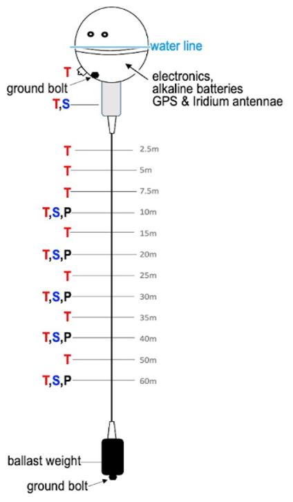
Figure 30Schematic of SASSIE Hydrobuoy 009, with sensors measuring ocean temperature (T), conductivity from which salinity is derived (S), and pressure (P). Other buoys had as many (or fewer) sensors (Table 7). This buoy did not include a drogue, whereas some others did.
Table 7Deployment location, time, and nominal depths (i.e., when the sensor string is hanging vertically) of available temperature, salinity, and pressure data of SASSIE Hydrobuoys, as well as whether the buoy had a drogue. As of March 2024, Hydrobuoys 002, 007, 008, and 009 were still recording.
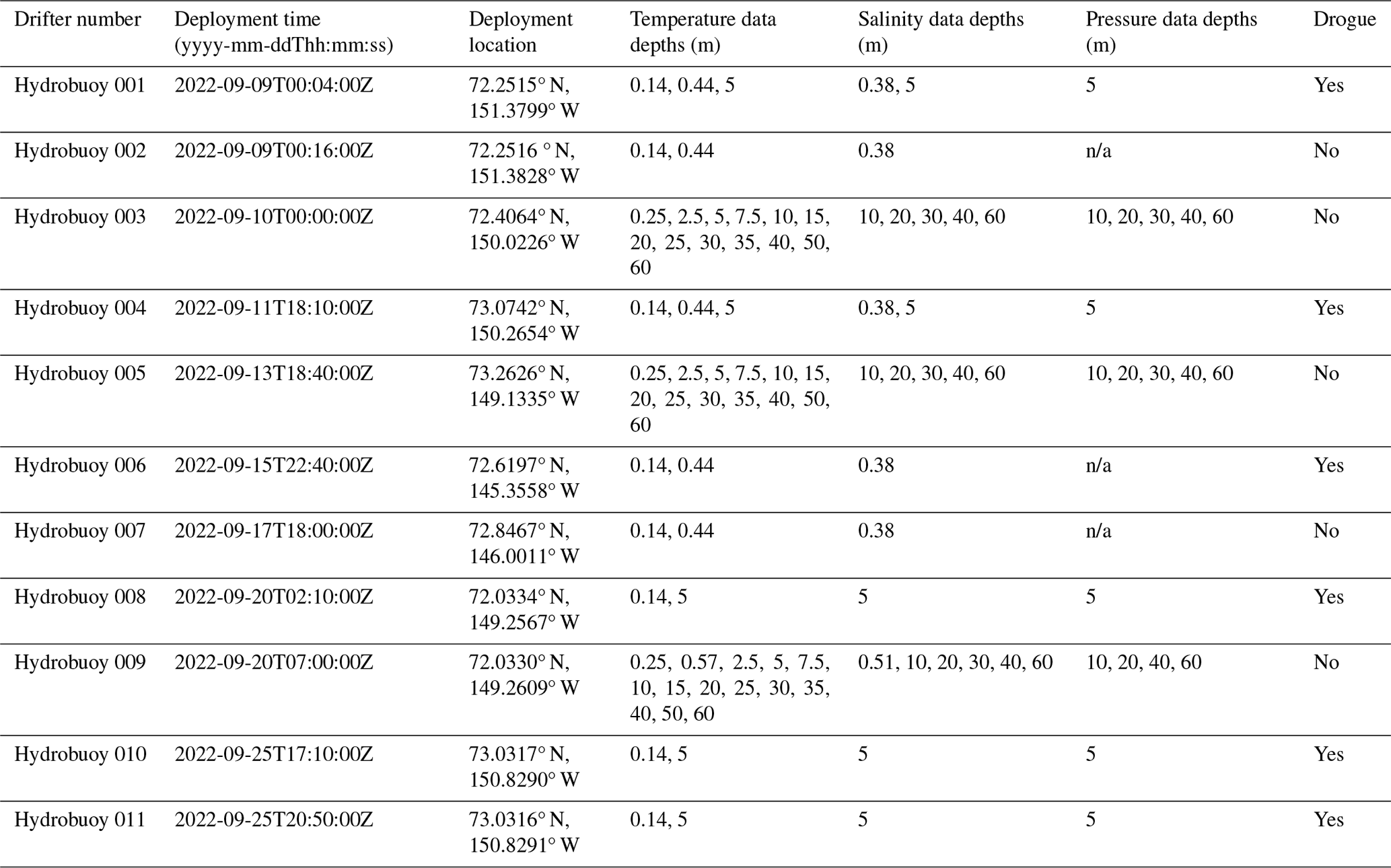
n/a: not applicable
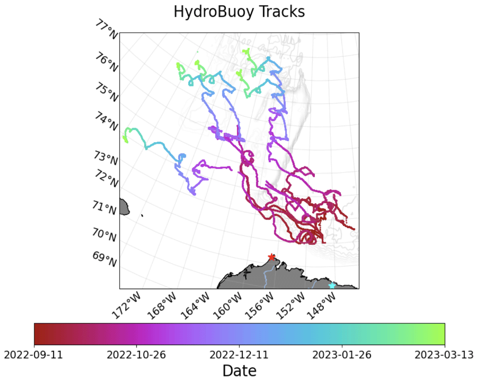
Figure 31Paths of the SASSIE Hydrobuoys throughout the SASSIE campaign and beyond. Shown are drift tracks from deployment in September 2022 through March 2023.
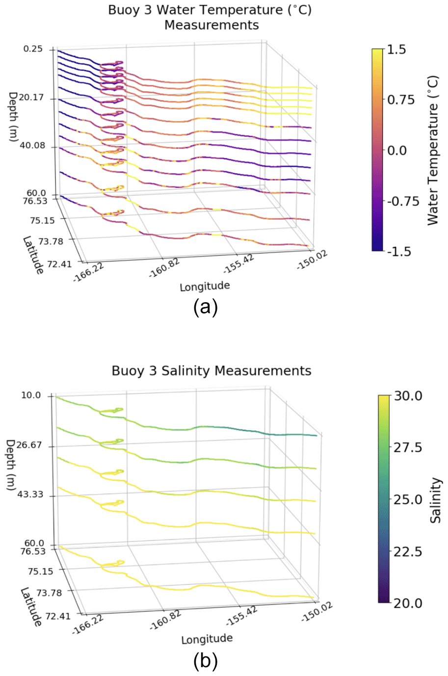
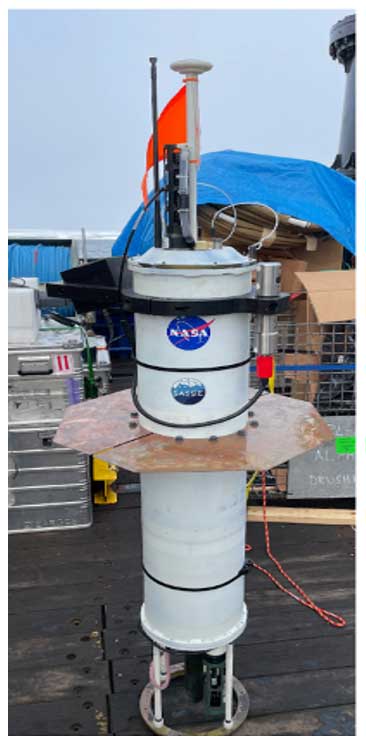
Figure 33The under-ice float (UIF) on the deck of R/V Woldstad before deployment. The float is about 2 m tall from the deck to the top of the antennas. Note CTDs at top and bottom of the float, the upward-looking camera mounted near the top of the float body on the left, and an ice-profiling sonar attached to the right-hand side. Photo credit: Jim Thomson.
Buoys with subsurface sensor strings also had ocean pressure sensors to determine changes in hydrography sensor depths owing to several reasons, namely (1) sensor string uplift owing to wind or ice pushing the surface hull, which makes the trailing sensor string rise up in the water column (this is very common); (2) sea ice ridging, which pulls up the sensor string into the ice (this often happens during winter); and (3) dragging on the ocean bottom (this generally happens when a buoy transits over the continental shelf, which did not happen during SASSIE). All buoys generally drifted west, northwest, and north after deployment (Fig. 31). All buoys performed well until they encountered ice (generally in late September through early December 2022), at which time communications stopped for many, but not all, buoys. As of September 2023, four buoys were still reporting, all of which had drifted northward to ∼86° N, 135° W over the Alpha Ridge. Four buoys were still reporting sea surface temperature (SST), three were reporting sea surface salinity (SSS), and one was reporting surface and subsurface temperature and salinity.
An example of buoy data is provided in Fig. 32. The ocean temperature data show gradual cooling at the surface and warm intrusions at depth that are likely summer Pacific water entering the southern Beaufort Sea from the northeastern Chukchi Sea. The ocean salinity data show declining stratification in the upper water column as fresh meltwater is mixed downward and salinified via ice growth and brine rejection.
2.2.5 Under-ice float (Shcherbina, 2023)
An under-ice float (UIF) is a heavily instrumented autonomous profiling vehicle based on the mixed-layer Lagrangian float design (e.g., D'Asaro, 2003). The SASSIE UIF was outfitted with two pumped Sea-Bird (SBE) 41CP CTDs mounted on the top and the bottom of the float, a narrow-beam upward-looking Valeport VA500 sonar, and an upward-looking camera for ice imaging (Fig. 33).
The UIF was deployed from R/V Woldstad on 10 September 2022 at 20:05 UTC at 73.12° N, 149.93° W within the marginal ice zone (Fig. 34). During its deployment, the float made frequent vertical profiles, surfacing when possible (i.e., when the sonar detected open water) to telemeter data. The last data transmission occurred on 23 October 2022.
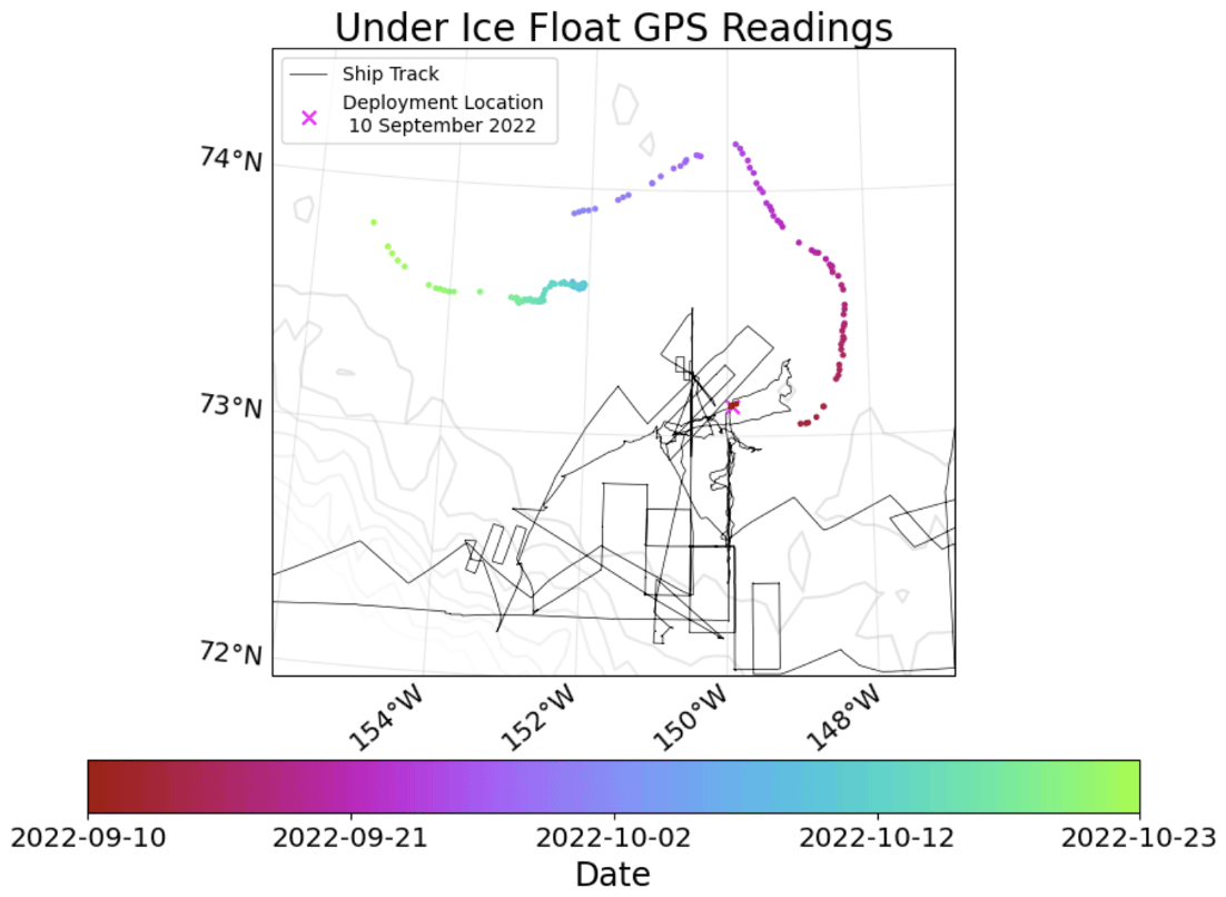
Figure 34GPS readings from the under-ice float colored according to date. The gaps in the record indicate the periods of heavy ice that prevented float surfacing. The black line denotes the ship track.
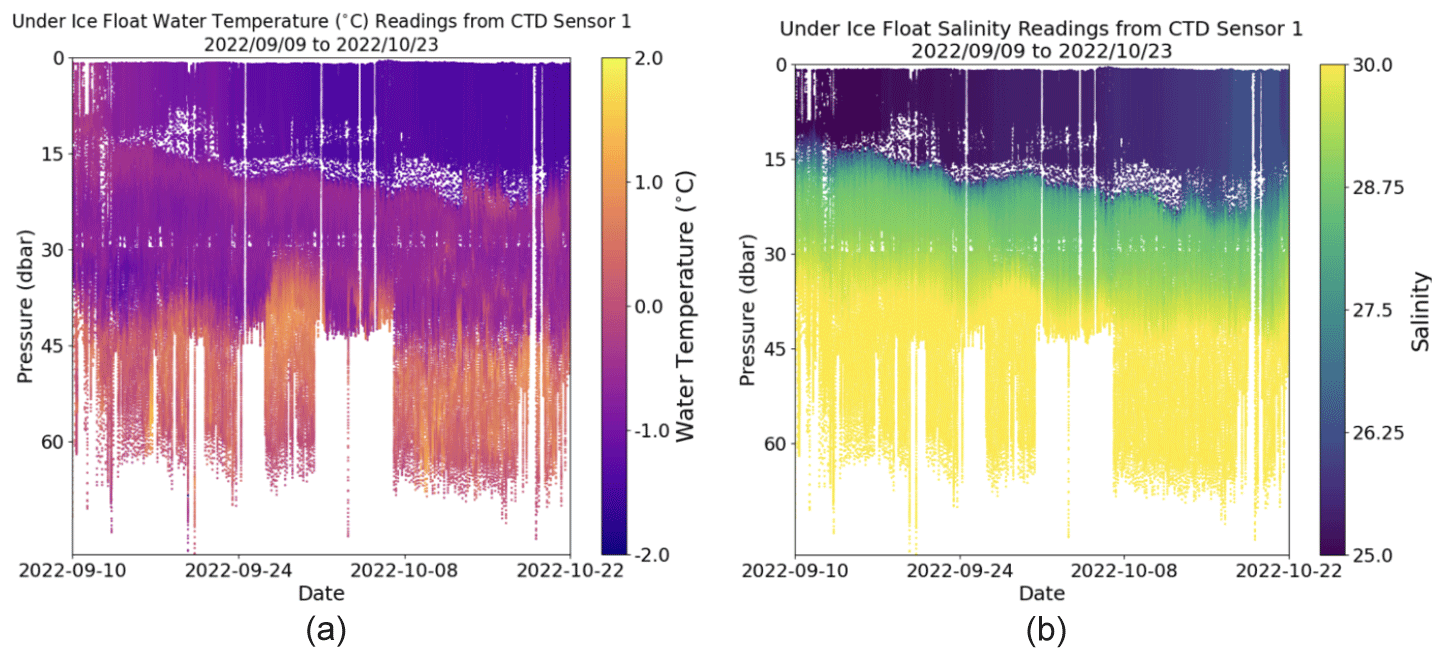
Figure 352D scatterplots of (a) water temperature and (b) salinity measurements from the UIF CTD sensor 1 (at the bottom of the UIF; Fig. 33) throughout its deployment.
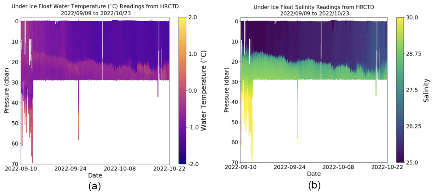
Figure 362D scatterplots of (a) water temperature and (b) salinity measurements from the UIF high-resolution CTD sensor throughout its deployment. The high-resolution CTD is seen attached to the top of the float in Fig. 33. Note the different color scale and vertical axes between this and the previous figure.
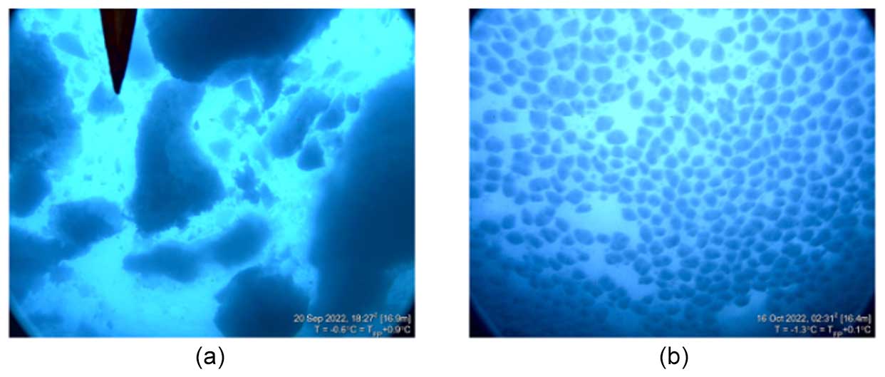
Figure 37Examples of UIF ice imagery. (a) Broken old ice (brash) commonly observed during the first half of the mission. (b) New pancake ice formation observed periodically during the freeze-up. Images are annotated in the lower-right corner with the date, time, UIF depth at that time, observed temperature, and its departure from the freezing point (TFP). The black shape visible in panel (a) is the UIF flag.
UIF profiling was focusing on the upper 40–50 m of the water column to resolve the evolution of the cold and fresh mixed layer in the later stages of summer ice melt and the transition to freeze-up (Fig. 35). Particular attention was paid to the upper meters under the ice or open water where vertical CTD resolution down to 1 cm was achieved through reduced profiling speed and increased sampling rate (Fig. 36). The frequency of the profiles varied through the course of the mission, but it was typically between 12 and 18 profiles per day (15 profiles per day on average). Periodically, the UIF spent time hovering 10–15 m below the surface, utilizing its sonar and camera to survey the ice topography and capture photos (Fig. 37).
The UIF CTD records (Figs. 35–36) show a general increase in salinity, decrease in temperature, and deepening of the mixed layer in September–October. These changes were due to entrainment of saltier pycnocline water accompanied by surface heat loss. Advective changes in the water mass structure were also evident below 30 m (within the pycnocline). Until 30 September, the mixed-layer temperature stayed > 0.1 °C above the freezing point. At that time, the ice cover remained fragmented and consisted of old brash ice (Fig. 37a). Even though the temperature approached freezing by October, new ice formation was intermittent. Calm weather periods allowed periodic formation of pancake (Fig. 37a) and nilas ice. These new ice formation events were interspersed with prolonged periods of open water and rough seas. Ice formation intensified and started to show signs of consolidation in the second half of October.
2.2.6 ALTO and ALAMO floats (Jayne, 2023)
Seven profiling floats (Table 8) manufactured by Marine Robotic Vehicles (MRV)-Systems were deployed during SASSIE. These floats provide autonomous profiles of ocean temperature and salinity and were set to sample over the upper 100 m. They thus provide information about SST, SSS, and thermal and haline stratification. The floats profile vertically by changing their buoyancy and drifting laterally with the local currents. Since the floats were sampling rapidly (multiple profiles per day) over the upper 100 m, their drift is a complex integration of upper-ocean current speed and direction.
Table 8Deployment dates and locations of the ALTO and ALAMO floats. Three additional ALAMO floats were deployed (two on 9 September 2022 and one on 10 September 2022) but did not collect any data.
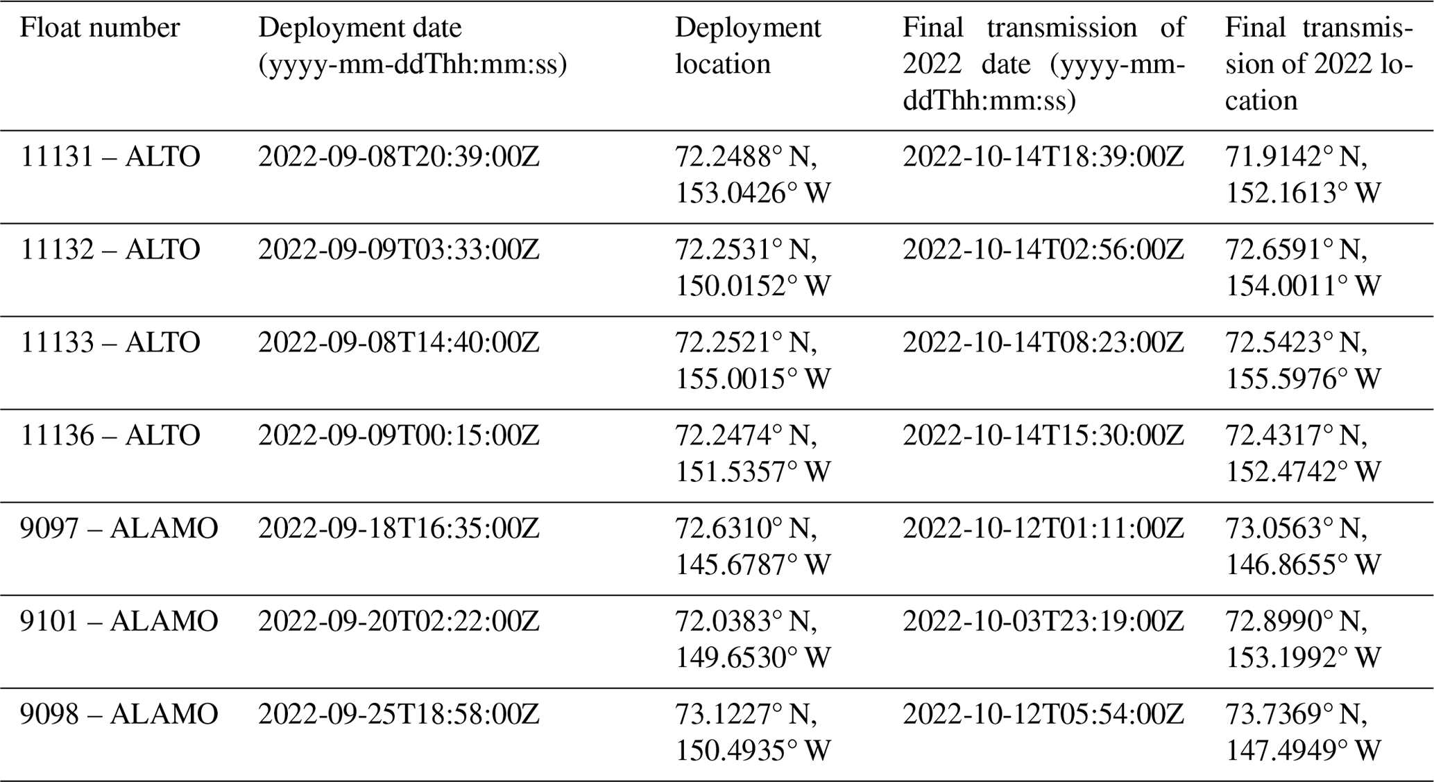
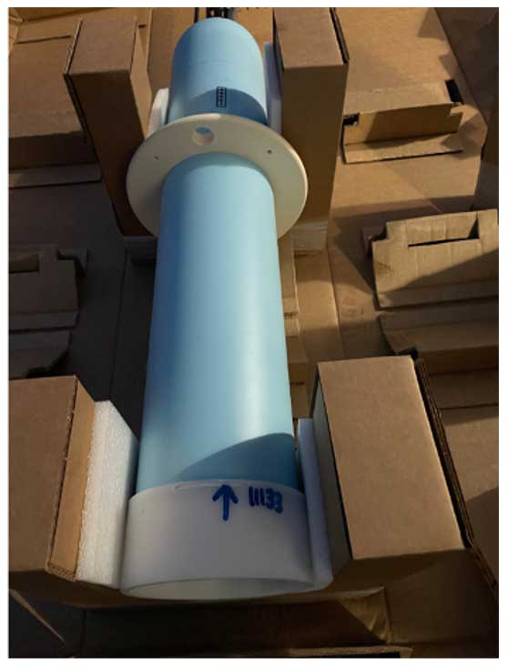
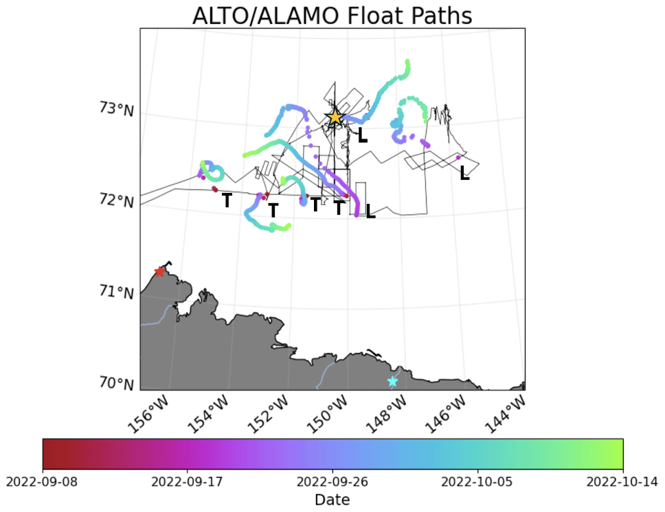
Figure 39Paths of the ALTO (designated “T”) and ALAMO (designated “L”) floats throughout the field campaign and colored by date. The path of float 9098 (measurements shown in Fig. 40) is marked by an orange star.
Four of the seven working floats were relatively larger (133 cm long, 16.5 cm, and 19.2 kg) ALTO floats (Fig. 38), and three were relatively smaller (91 cm long, 12.2 cm diameter, and 8.4 kg) ALAMO floats. All floats stopped reporting owing to advancing ice by late September through October 2022 (Fig. 39). The ALTO floats included an “ice avoidance” algorithm (e.g., Wong et al., 2020) with the goal of surviving winter. Unfortunately, none of these floats reported in summer 2023. The ALAMO floats did not include this feature to maximize data collection during freeze-up.
An example of float data is provided in Fig. 40. A clear signal of subsurface warm layers is evident, especially to the southeast at the start of the drift where warm summer Pacific Water is likely entering the Beaufort Sea from the northeastern Chukchi Sea. The data show a rather complex temperature profile that might also include warming from local radiative fluxes (i.e., a near-surface temperature maximum) which will be investigated using full hydrographic and meteorological analyses.
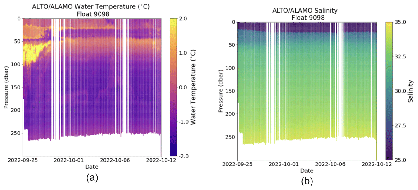
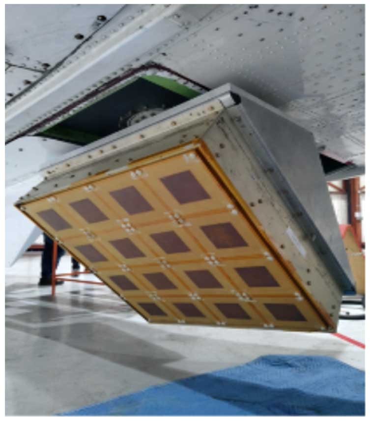
Figure 41PALS patch array antenna installed underneath the DC3-T Basler (BT-67) aircraft. The antenna is mechanically rotated 360° via a scanner motor (not seen) and covered with a radome before flight operations.
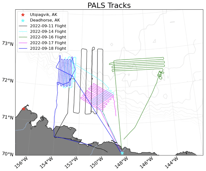
Figure 42Map of the PALS flights. Different colors indicate different flights (Table 9), as shown in the legend at the top left. Thin gray lines show bathymetry contours.
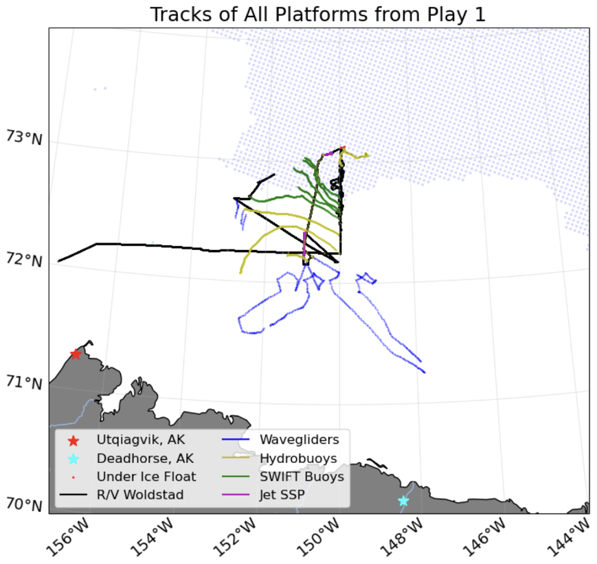
Figure 43A map showing the tracks of all six platforms during Play 1. Blue stippling indicates an ice concentration greater than 0 % on 11 September 2022, as determined from the MASIE-NH ice product.
2.3 PALS aircraft
To link in situ SSS measurements to SSS patterns across broader spatial scales, airborne measurements of SSS were made with the Jet Propulsion Laboratory (JPL) Passive/Active L-/S-band System (PALS) microwave radiometer (Wilson et al., 2001a, b; Yueh and Chaubell, 2011). The aircraft measurements provided broad-scale context and enabled quantification of SSS and SST, their horizontal gradients, and sea ice signals. PALS measures at the same L-band frequencies as the NASA Soil Moisture Active Passive (SMAP) satellite instrument, with significantly increased spatial resolution and accuracy over shorter timescales. PALS measures at 1.4 GHz with 24 MHz bandwidth and has the capability of measuring at 1.2 GHz with an 80 MHz bandwidth. The combination of these two frequencies significantly increases the sensitivity to salinity in cold waters. PALS can provide 300 to 1500 m horizontal resolution when flying at altitudes of 1 to 3 km. The airborne PALS radiometer has significantly smaller measurement noise compared to satellite radiometers because airborne platforms have far longer scene integration times and therefore a greater reduction in the uncorrelated measurement errors.
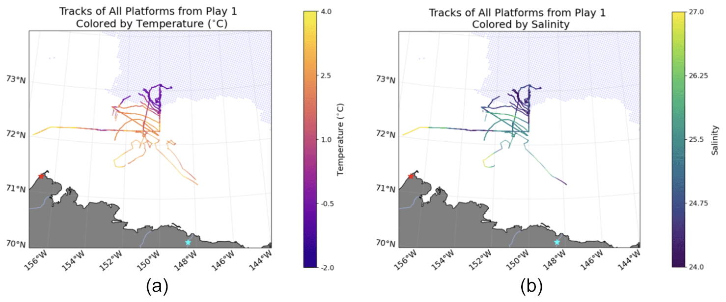
Figure 44(a) Temperature and (b) salinity recorded closest to the sea surface by each asset during Play 1 (except the UIF because it does not consistently make measurements near the sea surface). Blue stippling indicates an ice concentration greater than 0 % on 11 September 2022, as determined from the MASIE-NH ice product.
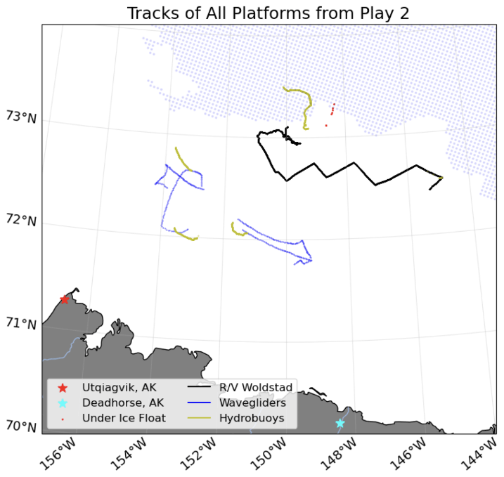
Figure 45A map showing the tracks of all six platforms deployed during Play 2. Blue stippling indicates an ice concentration greater than 0 % on 15 September 2022, as determined from the MASIE-NH ice product.
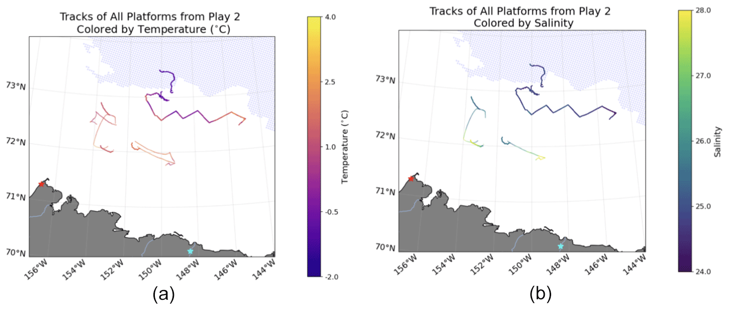
Figure 46(a) Temperature and (b) salinity recorded closest to the sea surface by each asset (except UIF) during Play 2. Blue stippling indicates an ice concentration greater than 0 % on 15 September 2022, as determined from the MASIE-NH ice product.
After averaging, PALS can theoretically measure SSS in cold waters (SST <5 °C) with 0.2–0.25 resolution over 1 km horizontal scales. During SASSIE, the instrument suite also included a compact wideband (750 MHz) C- and X-band radiometer to measure SST and ocean wind speed, respectively, at approximately 0.3 K and 1 m s−1 resolution. The PALS instrument also has an on-board combined infrared (IR) and visible imaging camera that covers a 45° swath. The IR camera provides radiometric temperatures for each point at 1.56 m × 1.95 m resolution per acquisition with <50 mK sensitivity when flying at an altitude of 1 km; the visible camera has 0.25 m × 0.33 m resolution when flying at an altitude of 1 km. For surveys over partial ice cover, the visible and IR imagery provide high-resolution estimates of ice concentration for comparison with and validation of the satellite-derived ice concentration. The combination of the embedded GPS and IMU modules with the dual visible and thermal camera capability provides time-stamped and geolocated radiometric measurements that can be synchronized with the PALS radiometer measurements.
PALS was installed in a Basler DC3-T aircraft operated by Kenn Borek Air Limited, a Canadian operator. Five PALS flights were made during SASSIE (Table 9); flights 1 and 3 were over R/V Woldstad, and flights 2, 4, and 5 were over Wave Gliders (Fig. 42).
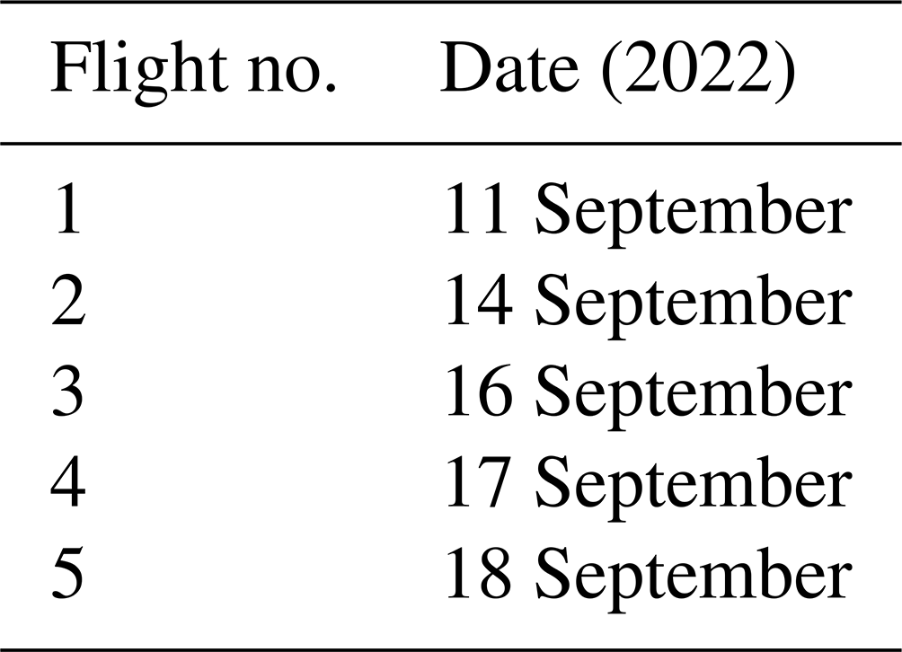
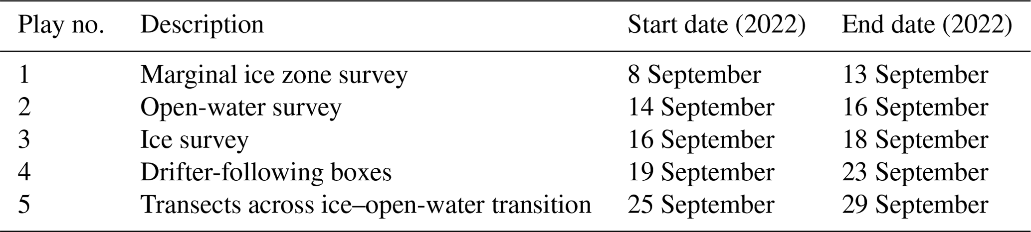
Table 11DOIs for each of the published SASSIE datasets plus additional references if available.
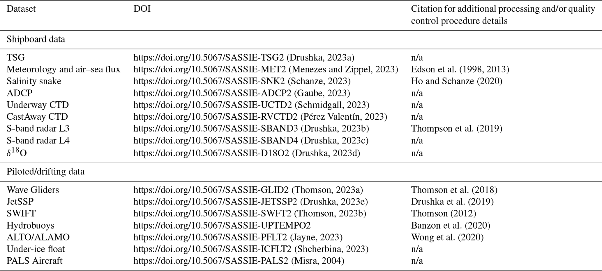
n/a: not applicable
The PALS airborne measurement data processing consists of converting measured uncalibrated counts to polarized microwave brightness temperature values at 1.2 and 1.4 GHz and ultimately converting those to SSS.
The initial calibration process from uncalibrated measured counts to brightness temperature (Tb) utilizes internal calibration sources present within the PALS radiometer (noise diode and reference load) that provide instantaneous gain and offset calibration coefficients. On-board temperature sensors allow constant tracking of the instrument temperature variations as the aircraft changes altitudes and outside temperature varies. PALS calibration also takes into account any potential scan-dependent variations within the data observed from sources such as the internal scan motor or the external radome. Another key data processing step is detecting and excising radio frequency interference (RFI) from the Tb measurements. During SASSIE flights, 1.2 GHz passive microwave data saw extreme RFI corruption, making the data almost unusable. The 1.4 GHz radiometer data were relatively free of RFI.
Airborne Tb measurements at 1.4 GHz see contributions from direct and reflected solar and galactic reflection, rain, RFI, SSS, SST, and ocean wind vectors or sea surface roughness. In order to derive salinity from brightness temperature, these other parameters need to be corrected for or removed. At a cold SST of less than 10 °C, the sensitivity of brightness temperature to salinity is nearly 3 times less than at tropical temperatures. SASSIE flew in rain-free conditions and took advantage of the 360° scan to correct for wind direction signatures and potential solar or galactic intrusions within the data. Although there was an on-board IR sensor to measure SST, due to mostly cloudy conditions, the IR data were contaminated, and the processing PALS data relied on ancillary SST values from satellite products. Wind speed and resulting white cap foam on the ocean surface is the most difficult contributor to correct. We use ancillary data such as advanced scatterometer (ASCAT) wind vectors, as well as on-board measurements from a C-/X-band radiometer, to derive relative wind speed trends observed during flight lines. Tb to SSS retrieval is done using the Klein–Swift model for the dielectric constant of seawater, though other models such as Meissner–Wentz and GW model were also tested. The absolute value in all models is slightly different at cold waters, but the relative variation in the salinity during flight lines is similar. We anchor derived SSS absolute values to “ground-truth” data obtained from the Wave Gliders. At the time of publication, PALS data were still undergoing processing.
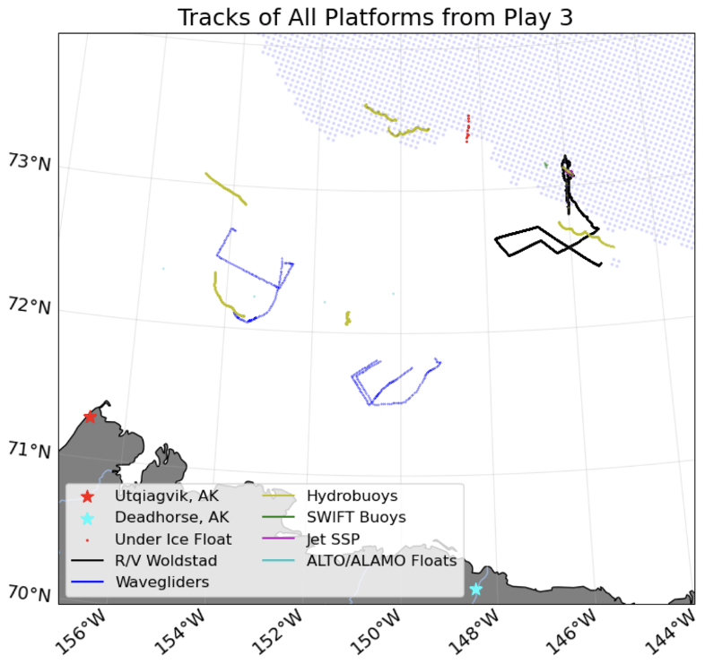
Figure 47A map showing the tracks of all six platforms during Play 3. Blue stippling indicates an ice concentration greater than 0 % on 17 September 2022, as determined from the MASIE-NH ice product.
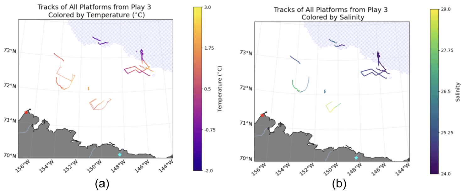
Figure 48(a) Temperature and (b) salinity recorded closest to the sea surface by each asset (except UIF) during Play 3. Blue stippling indicates an ice concentration greater than 0 % on 17 September 2022, as determined from the MASIE-NH ice product.
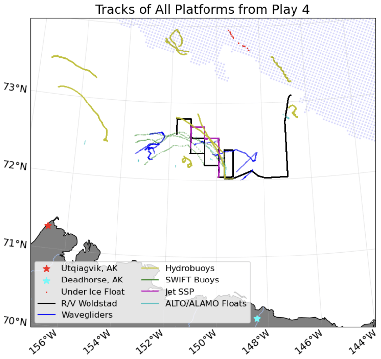
Figure 49A map showing the tracks of all six platforms during Play 4. Blue stippling indicates an ice concentration greater than 0 % on 21 September 2022, as determined from the MASIE-NH ice product.
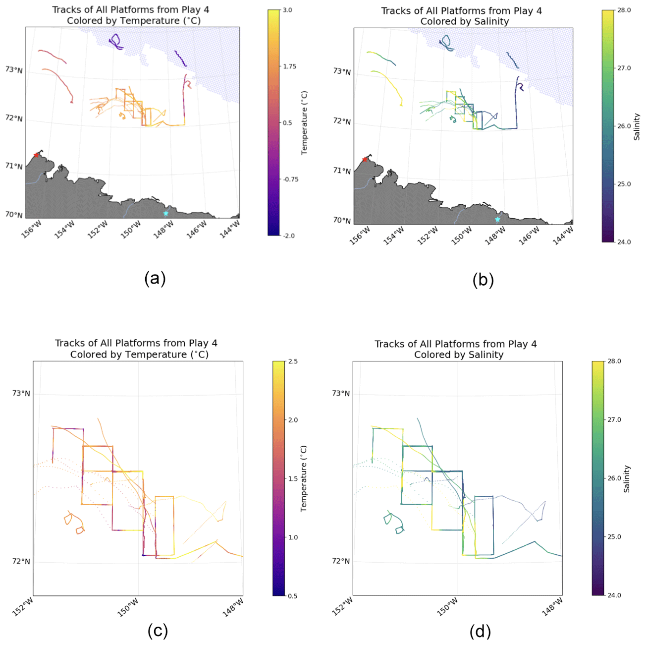
Figure 50(a) Temperature and (b) salinity recorded closest to the sea surface by each asset (except UIF) during Play 4. A zoomed-in view of the temperature (c) and salinity (d) recorded by the drifter following boxes is also shown. Blue stippling indicates an ice concentration greater than 0 % on 21 September 2022, as determined from the MASIE-NH ice product.
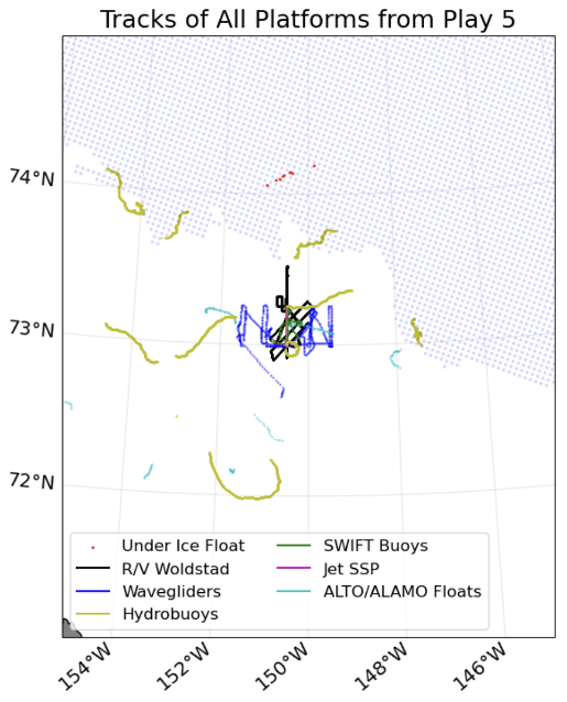
Figure 51A map showing the tracks of all six platforms during Play 5. Blue stippling indicates an ice concentration greater than 0 % on 27 September 2022, as determined from the MASIE-NH ice product.
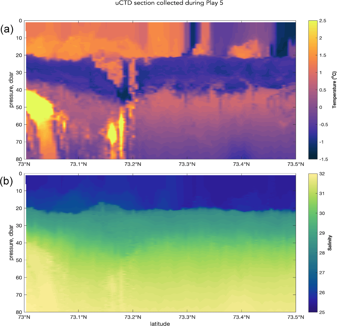
Figure 52(a) Temperature and (b) salinity collected with the uCTD along 150°30′ W during one section of Play 5 on 25 September. During this transect, sea ice was observed north of around 73.3° N, with open water observed to the south.
Table 11 gives information about where to access the data described in this paper. All datasets have been quality-controlled by the investigators who collected the dataset, and details about the processing of some of them are described in the papers listed in Table 11. The datasets are considered to be processed and calibrated (i.e., level 2, L2), except where indicated. Data are accessed using the DOIs listed in Table 11. The full SASSIE data archive is also accessible via PO.DAAC, https://podaac.jpl.nasa.gov/SASSIE/ (last access: 29 May 2024). Access to level 0 (L0) data can be obtained by contacting PO.DAAC at podaac@nasa.jpl.gov. Additional information about the Wave Glider, ALTO/ALAMO, and SWIFT datasets can be found at their respective DOIs under “Documentation”. All data files include CF-compliant metadata describing the instruments.
Code used to read the SASSIE data and generate the figures from this work is available as Jupyter Notebooks at https://github.com/lizwestbro/SASSIE_Data (last access: 6 September 2024) (https://doi.org/10.5281/zenodo.8327199, Westbrook, 2023).
The SASSIE cruise revolved around five major “Plays” (Table 10), each of which was essentially a mini-experiment that targeted a particular region, feature, or set of conditions using a tailored sampling strategy and suite of platforms. The shipboard and aircraft teams determined the location and strategy for each play based on local conditions such as weather, sea ice, presence of salinity, or temperature gradients, as well as relevance to the SASSIE objectives.
4.1 Play 1: marginal ice zone survey
Play 1 began as R/V Woldstad entered the MIZ (marginal ice zone) on 8 September, deploying five ALTO/ALAMO profiling floats, five Hydrobuoys, and five SWIFTs during the following days to capture the transition between open-ocean and moderate sea ice cover (Fig. 43). The ship focused primarily on the sea-ice-covered waters north of around 72°30′ N, while Wave Gliders and the aircraft captured open waters to the south. As the ship navigated through the heaviest ice cover of the expedition (estimated to be >60 % ice cover), the UIF was deployed, and water samples were collected at two ice stations to provide end-members for δ18O isotope analysis. Key observations included horizontal surface salinity differences of 2 to 3 from open water to ice, with strong surface salinity variability south of the ice edge and homogeneous salinities within ice-covered waters (Fig. 44).
4.2 Play 2: open-water survey
During Play 2, the ship surveyed south of the ice edge between 150 and 145° W, forming a zigzag pattern to maximize sampling of horizontal variability (Figs. 45 and 46). Winds and sea state were high, so profiling with the uCTD and JetSSP was limited. Conditions for flying were excellent, and the aircraft performed two surveys: a day over the Wave Gliders southwest of the ship in open water and another day in long east–west transects over the ship. The ship reached its easternmost point during this play.
4.3 Play 3: ice survey
On 16 September, R/V Woldstad entered the sea ice to avoid heavy seas as Typhoon Merbok hit the Bering Strait (Figs. 47 and 48). One Hydrobuoy was deployed, and two SWIFTs and JetSSP were deployed in moderate ice cover to examine small-scale gradients within the sea ice. Aircraft flights 3 and 4 (Table 9) over Wave Gliders to the southwest were carried out over 2 d.
4.4 Play 4: drifter-following boxes
Play 4 focused on capturing the spatiotemporal variability in a strong surface salinity front in open water. On 19 September, five assets were deployed in a north–south line across the gradient. As these assets drifted northwestward with the gyre circulation on the following 3 d, the ship steamed in a series of overlapping boxes around them (Fig. 49), collecting continuous uCTD measurements and deploying the JetSSP next to the ship to provide measurements from the surface down to ∼100 m. Additional SWIFTs were deployed on 21 and 22 September to target strong salinity gradients. Strong sub-mesoscale fronts were observed, with significant variability in both space and time (Fig. 50).
4.5 Play 5: transects across ice–open-water transition
The final play targeted the open-water–sea ice transition immediately prior to freeze-up (Fig. 51). Over 4 d, the ship made 14 consecutive transects along 150°30′ W, collecting uCTD measurements that captured the evolution of the upper ocean as it moved toward the freezing point. Wave Gliders made north–south transects on either side of the ship, and measurements with drifting assets and JetSSP were also collected. Figure 52 shows a single section of uCTD data. Notable features include a near-surface temperature maximum around 10–20 m depth that is maintained by the fresh surface layer; lateral variability above the pycnocline around 20 m depth, with the presence of temperature fronts coinciding with the transition into sea ice; and patchy Pacific summer water signals (warm water at 50–80 m depth) observed south of the ice edge.
| ADCP | Acoustic Doppler current profiler |
| AIS | Automatic identification system |
| ALTO | A profiling float manufactured by Marine Robotic Vehicles |
| ALAMO | Air-Launched Autonomous Micro-Observer |
| APL-UW | Applied Physics Laboratory, University of Washington |
| CDOM | Colored dissolved organic matter |
| CT | Conductivity and temperature |
| C-FLUOR probe | Turner Designs fluorescence probe |
| COARE | Coupled Ocean–Atmosphere Response Experiment |
| cCTD | CastAway conductivity–temperature–depth sensor |
| DCFS | Direct covariance flux system |
| DOI | Digital object identifier |
| ETOPO2 | National Centers for Environmental Information Topography and Bathymetry Global Relief Model |
| FDOM | Fluorescent dissolved organic matter |
| GeoTIFF | Geographical flag image file format |
| GPCTD | Glider payload conductivity–temperature–depth sensor |
| GPS | Global positioning system |
| IMU | Inertial motion unit |
| JetSSP | Jet-driven surface salinity profiler |
| MASIE | Multisensor Analyzed Sea Ice Extent (U.S. National Ice Center et al., 2010) |
| MIZ | Marginal ice zone |
| NASA | National Aeronautics and Space Administration |
| PALS | Passive Active L-/S-band System |
| PO.DAAC | Physical Oceanography Distributed Active Archive Center |
| RH | Relative humidity |
| R/V | Research vessel |
| SASSIE | Salinity and Stratification at the Sea Ice Edge |
| SBE | Sea-Bird Electronics |
| SMAP | Soil Moisture Active Passive |
| SSS | Sea surface salinity |
| SST | Sea surface temperature |
| SV3 | Surface vehicle model 3 |
| SWIFT | Surface Wave Instrument Floats with Tracking |
| TKE | Total kinetic energy |
| TSG | Thermosalinograph |
| cCTD | CastAway conductivity–temperature–depth sensor |
| uCTD | Underway conductivity–temperature–depth sensor |
| UIF | Under-ice float |
| WHOI | Woods Hole Oceanographic Institution |
The video supplement at https://drive.google.com/file/d/11IM3b4Lo2YtxySdYQVrksAA6JBkl4IyN/view?usp=sharing (Westbrook, 2024) shows a map covering the SASSIE from 12 August 2022 to 31 October 2022. Blue shading indicates an ice concentration greater than 0 % each day, as determined from the MASIE-NH ice product. Colored markers indicate the position of SASSIE assets. The video has 1 h time resolution.
The supplement related to this article is available online at: https://doi.org/10.5194/essd-16-4209-2024-supplement.
KD and PG led the SASSIE project, with KD leading through the cruise and PG leading the post-cruise work. KD wrote Sects. 1, 3, and 4 of the paper. EW co-wrote the paper and prepared the figures and code, with contributions from all co-authors. FMB and EW led the data publication. KD led the collection and processing of the TSG, JetSSP, S-band radar, and δ18O data. PG and CS led the collection and processing of the uCTD data. PG, EJR, and JT led the collection and processing of the ADCP data. PG and JP led the collection and processing of the cCTD data. SD and MS led the collection and processing of the Hydrobuoy data. MS organized the deployment of the ALAMO and ALTO float data. SF and SM led the collection and processing of the PALS data. VM and SZ led collection and processing of the meteorology and air–sea flux data. JT and EJR led the collection and processing of the Wave Glider and SWIFT data. JJS led the collection and processing of the salinity snake data. AS led the collection and processing of the under-ice float data.
The contact author has declared that none of the authors has any competing interests.
Publisher's note: Copernicus Publications remains neutral with regard to jurisdictional claims made in the text, published maps, institutional affiliations, or any other geographical representation in this paper. While Copernicus Publications makes every effort to include appropriate place names, the final responsibility lies with the authors.
The SASSIE Program has been supported by NASA. We thank Nadya Vinogradova-Shiffer of NASA for her support throughout the SASSIE program. We are grateful to the captains and crew of R/V Woldstad and to the Support Vessels of Alaska Inc., as well as the pilots of Kenn Borek Air Limited, for enabling us to collect these data. We thank Justin Burnett, Alex de Klerk, Léa Olivier, and Laëtitia Parc, for helping collect data on the SASSIE expedition, and Ian Fenty and Mehmet Ogut, for helping collect SASSIE aircraft data. ALAMO and ALTO floats were provided, and the data organized by Steven Jayne, Alexander Ekholm (WHOI), and Jeffrey Kerling (NAVOCEANO).
This research has been supported by the National Aeronautics and Space Administration (grant no. 80NSSC21K0832).
This paper was edited by Dagmar Hainbucher and reviewed by two anonymous referees.
Banzon, V., Smith, T. M., Steele, M., Huang, B., and Zhang, H.: Improved Estimation of Proxy Sea Surface Temperature in the Arctic, J. Atmos. Ocean. Tech., 37, 341–349, https://doi.org/10.1175/JTECH-D-19-0177.1, 2020.
Castro, S., Wick, G., and Steele, M.: Validation of satellite sea surface temperature analyses in the Beaufort Sea using UpTempO buoys, Remote Sens. Environ., 187, 458–475, https://doi.org/10.1016/j.rse.2016.10.035, 2016.
Cox, G. F. and Weeks, W. F.: Salinity variations in sea ice, J. Glaciol., 13, 109–120, 1974.
Crews, L., Lee, C. M., Rainville, L., and Thomson, J.: Direct observations of the role of lateral advection of sea ice meltwater in the onset of autumn freeze up, J. Geophys. Res.-Oceans, 127, e2021JC017775, https://doi.org/10.1029/2021JC017775, 2022.
D'Asaro, E. A.: Performance of autonomous Lagrangian floats, J. Atmos. Ocean. Tech., 20, 896–911, https://doi.org/10.1175/1520-0426(2003)020<0896:POALF>2.0.CO;2, 2003.
Dewey, S. R., Morison, J. H., and Zhang, J.: An Edge-Referenced Surface Fresh Layer in the Beaufort Sea Seasonal Ice Zone, J. Phys. Oceanogr., 47, 1125–1144, https://doi.org/10.1175/JPO-D-16-0158.1, 2017.
Drushka, K.: SASSIE Arctic Field Campaign Shipboard Thermosalinograph Data Fall 2022. Ver. 1, PO.DAAC, CA, USA [data set], https://doi.org/10.5067/SASSIE-TSG2, 2023a.
Drushka, K.: SASSIE Arctic Field Campaign Shipboard S-Band Radar Level 3 Data Fall 2022. Ver. 1, PO.DAAC, CA, USA [data set], https://doi.org/10.5067/SASSIE-SBAND3, 2023b.
Drushka, K.: SASSIE Arctic Field Campaign Shipboard S-Band Radar Level 4 Data Fall 2022. Ver. 1. PO.DAAC, CA, USA [data set], https://doi.org/10.5067/SASSIE-SBAND4, 2023c.
Drushka, K.: SASSIE Arctic Field Campaign Shipboard Delta-18O Data Fall 2022. Ver. 1, PO.DAAC, CA, USA [data set], https://doi.org/10.5067/SASSIE-D18O2, 2023d.
Drushka, K.: SASSIE Arctic Field Campaign Jet Surface Salinity Profiler Data Fall 2022. Ver. 1, PO.DAAC, CA, USA [data set], https://doi.org/10.5067/SASSIE-JETSSP2, 2023e.
Drushka, K., Asher, W. E., Jessup, A. T., Thompson, E. J., Iyer, S., and Clark, D.: Capturing fresh layers with the surface salinity profiler, Oceanography, 32, 76–85, https://doi.org/10.5670/oceanog.2019.215, 2019.
Edson, J. B., Fairall, C. W., Mestayer, P. G., and Larsen, S. E.: A study of the inertial-dissipation method for computing air-sea fluxes, J. Geophys. Res.-Oceans, 96, 10689–10711, https://doi.org/10.1029/91JC00886, 1991.
Edson J. B., Hinton, A. A., Prada, K. E., Hare, J. E., and Fairall, C. W.: Direct covariance flux estimates from mobile platforms at sea, J. Atmos. Ocean. Tech., 15, 547–562, https://doi.org/10.1175/1520-0426(1998)015<0547:DCFEFM>2.0.CO;2, 1998.
Edson, J. B., Jampana, V., Weller, R., A., Bigorre, S. P., Plueddemann, A. J., Fairall, C. W., Miller, S. D., Mahrt, L., Vickers, D., and Hersbach, H.: On the exchange of momentum over the open ocean, J. Phys. Oceanogr., 43, 1589–1610, https://doi.org/10.1175/JPO-D-12-0173.1, 2013.
Fairall, C. W. and Markson, R.: Mesoscale variations in surface stress, heat fluxes, and drag coefficient in the marginal ice zone during the 1983 Marginal Ice Zone Experiment, J. Geophys. Res.-Oceans, 92, 6921–6932, https://doi.org/10.1029/JC092iC07p06921, 1987.
Fairall, C. W., Edson, J. B., Larsen, S. E., and Mestayer, P. G.: Inertial-dissipation air-sea flux measurements: a prototype system using real time spectral computations, J. Atmos. Ocean. Tech., 7, 425–453, https://doi.org/10.1175/1520-0426(1990)007<0425:IDASFM>2.0.CO;2, 1990.
Gaube, P.: SASSIE Arctic Field Campaign Shipboard ADCP Data Fall 2022. Ver. 1, PO.DAAC, CA, USA [data set], https://doi.org/10.5067/SASSIE-ADCP2, 2023.
Haykin, S., Currie, B. W., Lewis, E. O., and Nickerson, K. A.: Surface-based radar imaging of sea ice, Proc. IEEE, 73, 233–251, https://doi.org/10.1109/PROC.1985.13136, 1985.
Ho, D. T. and Schanze, J. J.: Precipitation-Induced Reduction in Surface Ocean pCO2: Observations From the Eastern Tropical Pacific Ocean, Geophys. Res. Lett., 47, e2020GL088252, https://doi.org/10.1029/2020GL088252, 2020.
Jackson, J. M., Carmack, E. C., McLaughlin, F. A., Allen, S. E., and Ingram, R. G.: Identification, characterization, and change of the near-surface temperature maximum in the Canada Basin, 1993–2008, J. Geophys. Res.-Oceans, 115, C05021, https://doi.org/10.1029/2009JC005265, 2010.
Jayne, S.: SASSIE Arctic Field Campaign ALTO/ALAMO Profiling Float Data Fall 2022. Ver. 1, PO.DAAC, CA, USA [data set], https://doi.org/10.5067/SASSIE-PFLT2, 2023.
Lannuzel, D., Tedesco, L., Van Leeuwe, M., Campbell, K., Flores, H., Delille, B., Miller, L., Stefels, J., Assmy, P., Bowman, J., and Brown, K.: The future of Arctic sea-ice biogeochemistry and ice-associated ecosystems, Nat. Clim. Chang., 10, 983–992, https://doi.org/10.1038/s41558-020-00940-4, 2020.
Lansard, B., Mucci, A., Miller, L. A., Macdonald, R. W., and Gratton, Y.: Seasonal variability of water mass distribution in the southeastern Beaufort Sea determined by total alkalinity and δ18O, J. Geophys. Res.-Oceans, 117, C03003, https://doi.org/10.1029/2011JC007299, 2012.
Lund, B., Graber, H. C., Persson, P. O., Smith, M., Doble, M., Thomson, J., and Wadhams, P.: Arctic sea ice drift measured by shipboard marine radar, J. Geophys. Res.-Oceans, 123, 4298–4321, https://doi.org/10.1029/2018JC013769, 2018.
Menezes, M. and Zippel, S.: SASSIE Arctic Field Campaign Shipboard Meteorology Data Fall 2022. Ver. 1, PO.DAAC, CA, USA [data set], https://doi.org/10.5067/SASSIE-MET2, 2023.
Misra, S.: SASSIE Arctic Field Campaign PALS Data Fall 2022. Ver. 1, PO.DAAC, CA, USA [data set], https://doi.org/10.5067/SASSIE-PALS2, 2024.
Ogut, M., Misra, S., Bosch-Lluis, X., Ramos, I., Williamson, R., Chae, C. S., Colliander, A., and Yueh, S.: Demonstration of a Combined Active/Passive L-Band Microwave Remote Sensing Airborne Instrument, IEEE J. Sel. Top. Appl. Earth Obs., 17, 11134–11145, https://doi.org/10.1109/JSTARS.2024.3404852, 2024.
Pérez Valentín, J.: SASSIE Arctic Field Campaign Castaway Data Fall 2022. Ver. 1, PO.DAAC, CA, USA [data set], https://doi.org/10.5067/SASSIE-RVCTD2, 2023.
Persson, P. O. G., Blomquist, B., Guest, P., Stammerjohn, S., Fairall, C., Rainville, L., Lund, B., Ackley, S., and Thomson, J.: Shipboard observations of the meteorology and near-surface environment during autumn freeze up in the Beaufort/Chukchi Seas, J. Geophys. Res.-Oceans, 123, 4930–4969, https://doi.org/10.1029/2018JC013786, 2018.
Schanze, J.: SASSIE Arctic Field Campaign Shipboard Salinity Snake Data Fall 2022. Ver. 1, PO.DAAC, CA, USA [data set], https://doi.org/10.5067/SASSIE-SNK2, 2023.
Schlundt, M., Farrar, J. T., Bigorre, S. P., Plueddemann, A. J., and Weller, R. A.: Accuracy of wind observations from open-ocean buoys: Correction for flow distortion, J. Atmos. Ocean. Tech., 37, 687–703, https://doi.org/10.1175/JTECH-D-19-0132.1, 2020.
Schmidgall, C.: SASSIE Arctic Field Campaign Shipboard Underway CTD Data Fall 2022. Ver. 1, PO.DAAC, CA, USA [data set], https://doi.org/10.5067/SASSIE-UCTD2, 2023.
Shcherbina, A.: SASSIE Arctic Field Campaign Under-Ice Float Data Fall 2022. Ver. 1, PO.DAAC, CA, USA [data set], https://doi.org/10.5067/SASSIE-ICFLT2, 2023.
Smith, M., Stammerjohn, S., Persson, O., Rainville, L., Liu, G., Perrie, W., Robertson, R., Jackson, J., and Thomson, J.: Episodic Reversal of Autumn Ice Advance Caused by Release of Ocean Heat in the Beaufort Sea, J. Geophys. Res.-Oceans, 123, 3164–3185, https://doi.org/10.1002/2018JC013764, 2018.
Steele, M.: SASSIE Arctic Field Campaign Drifter Hydrography Data Fall 2022. Ver. 1, PO.DAAC, CA, USA [data set], https://doi.org/10.5067/SASSIE-UPTEMPO2, 2023.
Stroeve, J. and Notz, D.: Changing state of Arctic sea ice across all seasons, Environ. Res. Lett., 13, 103001, https://doi.org/10.1088/1748-9326/aade56, 2018.
Stroeve, J. C., Markus, T., Boisvert, L., Miller, J., and Barrett, A.: Changes in Arctic melt season and implications for sea ice loss, Geophys. Res. Lett., 41, 1216–1225, https://doi.org/10.1002/2013GL058951, 2014.
Thompson, E. J., Asher, W. E., Jessup, A. T., and Drushka, K.: High-resolution rain maps from an X-band marine radar and their use in understanding ocean freshening, Oceanography, 32, 58–65, https://doi.org/10.5670/oceanog.2019.213, 2019.
Thomson, J.: Observations of wave breaking dissipation from a SWIFT drifter, J. Atmos. Ocean. Tech., 29, 1866–1882, https://doi.org/10.1175/JTECH-D-12-00018.1, 2012.
Thomson, J.: SASSIE Arctic Field Campaign Wave Glider Data Fall 2022. Ver. 1, PO.DAAC, CA, USA [data set], https://doi.org/10.5067/SASSIE-GLID2, 2023a.
Thomson, J.: SASSIE Arctic Field Campaign SWIFT Data Fall 2022. Ver. 1, PO.DAAC, CA, USA, [data set], https://doi.org/10.5067/SASSIE-SWIFT2, 2023b.
Thomson, J. and Girton, J.: Sustained measurements of Southern Ocean air-sea coupling from a Wave Glider autonomous surface vehicle, Oceanography, 30, 104–109, https://doi.org/10.5670/oceanog.2017.228, 2017.
Thomson, J., Girton, J., Jha, R., and Trapani, A.: Measurements of Directional Wave Spectra and Wind Stress from a Wave Glider Autonomous Surface Vehicle, J. Atmos. Ocean. Tech., 35, 347–363, https://doi.org/10.1175/JTECH-D-17-0091.1, 2018.
U.S. National Ice Center, Fetterer, F., Savoie, M., Helfrich, S., and Clemente-Colón, P.: Multisensor Analyzed Sea Ice Extent – Northern Hemisphere (MASIE-NH), Version 1 4km. Boulder, Colorado USA, National Snow and Ice Data Center [data set], https://doi.org/10.7265/N5GT5K3K, 2010.
Westbrook, E.: lizwestbro/SASSIE_Data: SASSIE Data Visualization – No Ice Mapping (v1.0.0-alpha), Zenodo [code], https://doi.org/10.5281/zenodo.8308513, 2023.
Westbrook, E.: SASSIE assets and sea ice movie, Google [video], https://drive.google.com/file/d/11IM3b4Lo2YtxySdYQVrksAA6JBkl4IyN/view?usp=sharing, last access: 29 May 2024.
Wilson, W. J., Yueh, S. H., Dinardo, S. J., Chazanoff, S. L., Kitiyakara, A., Li, F. K., and Rahmat-Samii, Y.: Passive active L-and S-band (PALS) microwave sensor for ocean salinity and soil moisture measurements, IEEE T. Geosci. Remote, 39, 1039–1048, https://doi.org/10.1109/36.921422, 2001a.
Wilson, W. J., Yueh, S. H., Li, F. K., Dinardo, S., Chao, Y., Koblinsky, C., Lagerloef, G., and Howden, S.: Ocean surface salinity remote sensing with the JPL Passive/Active L-/S-band (PALS) microwave instrument, in: IGARSS 2001. Scanning the Present and Resolving the Future, Proceedings, IEEE 2001 International Geoscience and Remote Sensing Symposium, Cat. No. 01CH37217, 2, 937–939, https://doi.org/10.1109/IGARSS.2001.976686, 2001b.
Wong, A. P., Wijffels, S. E., Riser, S. C., Pouliquen, S., Hosoda, S., Roemmich, D., Gilson, J., Johnson, G. C., Martini, K., Murphy, D. J., and Scanderbeg, M.: Argo data 1999–2019: Two million temperature-salinity profiles and subsurface velocity observations from a global array of profiling floats, Front. Marine Sci., 7, 700, https://doi.org/10.3389/fmars.2020.00700, 2020.
Yueh, S. H. and Chaubell, J.: Sea surface salinity and wind retrieval using combined passive and active L-band microwave observations, IEEE T. Geosci. Remote, 50, 1022–1032, https://doi.org/10.1109/TGRS.2011.2165075, 2011.