PM_2.5 concentrations based on near-surface visibility in the Northern Hemisphere from 1959 to 2022

Long-term PM_2.5 data are essential for the atmospheric environment, human health, and climate change. PM_2.5 measurements are sparsely distributed and of short duration. In this study, daily PM_2.5 concentrations are estimated using a machine learning method for the period from 1959 to 2022 in the Northern Hemisphere based on near-surface atmospheric visibility. They are extracted from the Integrated Surface Database (ISD). Daily continuous monitored PM_2.5 concentration is set as the target, and near-surface atmospheric visibility and other related variables are used as the inputs. A total of 80 % of the samples of each site are the training set, and 20 % are the testing set. The training result shows that the slope of linear regression with a 95 % confidence interval (CI) between the estimated PM_2.5 concentration and the monitored PM_2.5 concentration is 0.955 [0.955, 0.955], the coefficient of determination (R²) is 0.95, the root mean square error (RMSE) is 7.2 µg m⁻³, and the mean absolute error (MAE) is 3.2 µg m⁻³. The test result shows that the slope within a 95 % CI between the predicted PM_2.5 concentration and the monitored PM_2.5 concentration is 0.864 [0.863, 0.865], the R² is 0.79, the RMSE is 14.8 µg m⁻³, and the MAE is 7.6 µg m⁻³. Compared with a global PM_2.5 concentration dataset derived from a satellite aerosol optical depth product with 1 km resolution, the slopes of linear regression on the daily (monthly) scale are 0.817 (0.854) from 2000 to 2021, 0.758 (0.821) from 2000 to 2010, and 0.867 (0.879) from 2011 to 2022, indicating the accuracy of the model and the consistency of the estimated PM_2.5 concentration on the temporal scale. The interannual trends and spatial patterns of PM_2.5 concentration on the regional scale from 1959 to 2022 are analyzed using a generalized additive mixed model (GAMM), suitable for situations with an uneven spatial distribution of monitoring sites. The trend is the slope of the Theil–Sen estimator. In Canada, the trend is −0.10 µg m⁻³ per decade, and the PM_2.5 concentration exhibits an east–high to west–low pattern. In the United States, the trend is −0.40 µg m⁻³ per decade, and PM_2.5 concentration decreases significantly after 1992, with a trend of −1.39 µg m⁻³ per decade. The areas of high PM_2.5 concentration are in the east and west, and the areas of low PM_2.5 concentration are in the central and northern regions. In Europe, the trend is −1.55 µg m⁻³ per decade. High-concentration areas are distributed in eastern Europe, and the low-concentration areas are in northern and western Europe. In China, the trend is 2.09 µg m⁻³ per decade. High- concentration areas are distributed in northern China, and the low-concentration areas are distributed in southern China. The trend is 2.65 µg m⁻³ per decade up to 2011 and −22.23 µg m⁻³ per decade since 2012. In India, the trend is 0.92 µg m⁻³ per decade. The concentration exhibits a north–high to south–low pattern, with high-concentration areas distributed in northern India, such as the Ganges Plain and Thar Desert, and the low-concentration area in the Deccan Plateau. The trend is 1.41 µg m⁻³ per decade up to 2013 and −23.36 µg m⁻³ per decade from 2014. The variation in regional PM_2.5 concentrations is closely related to the implementation of air quality laws and regulations. The daily site-scale PM_2.5 concentration dataset from 1959 to 2022 in the Northern Hemisphere is available at the National Tibetan Plateau/Third Pole Environment Data Center (https://doi.org/10.11888/Atmos.tpdc.301127) (Hao et al., 2024).

1 Introduction

Fine particulate matter (PM_2.5) refers to particulate matter suspended in air with an aerodynamic diameter of less than 2.5 µm. PM_2.5 has various shapes and is composed of complex components, such as inorganic salts (e.g., sulfate, nitrate, and ammonium), as well as organic carbon and elemental carbon, metallic elements, and organic compounds (Chen et al., 2020; Fan et al., 2021). PM_2.5 can be emitted directly into the atmosphere (Viana et al., 2008; Zhang et al., 2019) and generated through photochemical reactions and transformations (Guo et al., 2014). PM_2.5 exhibits high concentrations near emission sources, which gradually decreases with distance. Due to the smaller size and longer life span compared with coarse particulate matter, PM_2.5 can be transported over long distances by atmospheric movements, leading to wide-ranging impacts. Studies indicate that regional transport contributes significantly to local PM_2.5 concentration (Wang et al., 2014; Chen et al., 2020).

PM_2.5 reduces atmospheric visibility and facilitates the formation of fog and haze conditions (Fan et al., 2021). Direct and indirect effects of PM_2.5 on solar radiation in the atmosphere (Albrecht, 1989; Ramanathan et al., 2001; Bergstrom et al., 2007; Chen et al., 2022) alter the energy balance and the number of condensation nuclei, thereby influencing atmospheric circulation and the water cycle (Wang et al., 2012; Liao et al., 2015; Samset et al., 2019; Li et al., 2022).

PM_2.5 is also known as respirable particulate matter. Due to its complex composition, PM_2.5 may carry toxic substances that can significantly impair human health. The World Health Organization states explicitly that PM_2.5 is more harmful than coarse particles, and long-term exposure to high PM_2.5 concentrations increases the risk of respiratory diseases, cardiovascular diseases, and lung cancer (Lelieveld et al., 2015), regardless of a country's development status. A Global Burden of Diseases study reveals that exposure to environmental PM_2.5 causes thousands of deaths and millions of lung diseases annually (Chafe et al., 2014; Kim et al., 2015; Cohen et al., 2017).

PM_2.5 is an important parameter for assessing particulate matter pollution and air quality (Wang et al., 2012). PM_2.5 can lead to soil acidification, water pollution, disruption of plant respiration, and ecological degradation (Wu and Zhang, 2018; Liu et al., 2019). Due to globalization and economic integration, preventing and controlling particulate matter pollution is a challenge at city, country, and global scales.

Therefore, long-term PM_2.5 concentration data are needed for studies on the environment, human health, and climate change. At present, ground-based measurements, chemical models, and estimations of alternatives are the primary sources of PM_2.5 concentration data.

Ground-based measurements are the most effective means of measuring PM_2.5 concentration. PM_2.5 monitoring has been ongoing since the 1990s in North America and Europe (Van Donkelaar et al., 2010), and large-scale PM_2.5 monitoring has been implemented in other regions since 2000, including China in 2013 (Liu et al., 2017). As a result, the records for PM_2.5 concentration are short, with only a few years of data available in many countries. The scarcity of PM_2.5 measurements makes it challenging to provide long-term historical data for research.

Many studies have employed statistical methods and machine learning and deep learning methods to estimate PM_2.5 concentrations based on aerosol optical depth. Van Donkelaar et al. (2021) utilized satellite aerosol optical depth data, aerosol vertical structure of chemical transport models, and ground-level measurements to estimate monthly PM_2.5 concentrations and their uncertainties over global land from 1998 to 2019, and there are several related studies (Van Donkelaar et al., 2010; Boys et al., 2014; Van Donkelaar et al., 2015, 2016; Hammer et al., 2020). Many studies have been conducted at the regional scale, such as in the United States (Beckerman et al., 2013), China (Wei et al., 2019b; Xue et al., 2019; Wei et al., 2020; He et al., 2021; Wei et al., 2021), and India (Mandal et al., 2020). Although the PM_2.5 concentrations derived from satellite retrievals have high spatial coverage, there are some limitations that need to be considered. Aerosol optical depth describes the column properties of aerosol, while PM_2.5 concentration describes the near-surface properties of aerosol. Therefore, aerosol vertical structure is crucial in establishing the relationship between the two. The daily representativeness is also considerable, as PM_2.5 concentration is continuously monitored, while the daily frequency of satellite observations is low (one to two times). Surface types, cloud conditions (Wei et al., 2019a), and resolution (Nagaraja Rao et al., 1989; Hsu et al., 2017) affect the accuracy of satellite products, thereby increasing uncertainty of estimation of PM_2.5 concentration.

Reanalysis datasets provide estimates of long-term particulate matter concentrations. The Modern-Era Retrospective Analysis for Research and Applications version 2 (MERRA-2) is an excellent reanalysis dataset from NASA that uses the Goddard Earth Observing System version 5 (GEOS-5). It has been providing global PM_2.5 data since 1980 (Buchard et al., 2015, 2016, 2017; Gelaro et al., 2017; Sun et al., 2019). There are some emission inventories in the aerosol model, including volcanic material; monthly biomass burning from 1980 to 1996; monthly SO₂, SO₄, particulate organic matter (POM), and black carbon (BC) from 1997 to 2009; annual anthropogenic SO₂ between 100 and 500 m above the surface from 1980 to 2008; and annual anthropogenic SO₄, BC, and POM concentrations from 1980 to 2006. In assimilation systems, satellite aerosol products from MISR and MODIS Aqua/Terra are assimilated after 2000. Another reanalysis dataset is the Copernicus Atmosphere Monitoring Service (CAMS) global reanalysis, which is a global reanalysis dataset of the atmospheric composition produced by the European Centre for Medium-Range Weather Forecasts (ECMWF). It has provided PM_2.5 data since 2003 (Che et al., 2014; Inness et al., 2019). Although reanalysis provides long-term PM_2.5 data, the uncertainty in emission inventories increases the uncertainty in PM_2.5 concentration (Granier et al., 2011). The validation of the reanalysis based on emission inventories shows that PM_2.5 concentration is still overestimated or underestimated in some regions (Buchard et al., 2017; Ali et al., 2022; Jin et al., 2022). The assimilation of aerosol optical depth products improves the aerosol column properties (Buchard et al., 2017), thereby improving the estimation of surface PM_2.5 concentration, as it to some extent constrains the vertical structure of aerosols. However, the lack of high-spatiotemporal-resolution emission inventories and long-term assimilation data greatly limits the accuracy of surface PM_2.5 concentrations.

Another alternative for estimating PM_2.5 concentrations is the near-surface atmospheric horizontal visibility, which is the maximum distance at which observers with normal visual acuity can discern target contours under current weather conditions. In addition to manual observations, automated visibility measurement has been implemented early, typically relying on the aerosol scattering principle (Wang et al., 2009; Zhang et al., 2020). Both visibility and PM_2.5 concentration are measurements of near-surface aerosols. They describe atmospheric horizontal transparency and are used to describe atmospheric pollution. Long-term visibility records have been used to quantify long-term aerosol properties (Molnár et al., 2008; Wang et al., 2009; Zhang et al., 2017, 2020). Visibility observation stations are densely distributed across the world. Compared to satellite retrievals, visibility observations have longer historical records dating back to the early 20th century (Boers et al., 2015), are not affected by cloud interference, and provide continuous measurements.

Visibility has been used as a proxy for PM_2.5 concentration (Huang et al., 2009) and for the estimation of PM_2.5 concentration (Liu et al., 2017; Li et al., 2020; Singh et al., 2020). Singh et al. (2020) analyzed air quality in east Africa from 1974 to 2018 using visibility data. Liu et al. (2017) developed a statistical model and utilized ground-level visibility data to estimate long-term PM_2.5 concentrations in China from 1957 to 1964 and 1973 to 2014. Gui et al. (2020) proposed a method to establish a virtual ground observation network for PM_2.5 concentration in China using extreme gradient boosting modeling in 2018. Zeng et al. (2021) used LightGBM to establish a virtual network for hourly PM_2.5 concentrations in China in 2017. Zhong et al. (2021, 2022) used LightGBM to predict 6 h PM_2.5 concentrations based on visibility, temperature, and relative humidity in China from 1960 to 2020. Meng et al. (2018) utilized a random forest model to estimate the daily PM_2.5 components in the United States from 2005 to 2015. These studies have provided various methods for estimating PM_2.5 using visibility data. However, some have only focused on methodological innovations without providing long-term trends in PM_2.5 concentration. Other studies offer long-term trends, but the primary focus is at an urban or national scale. There are few studies on long-term and high-temporal-resolution PM_2.5 concentration at the global scale or across different countries.

This study uses a convenient, accurate, and easily understandable machine learning approach to estimate daily PM_2.5 concentrations based on visibility at 5023 land-based sites from 1959 to 2022. First, we build a machine learning model and then analyze the importance of the variables. Second, we evaluate the model's performance and predictive ability. Third, we discuss the errors and limitations of the dataset. Fourth, we compare the estimated PM_2.5 concentration with the other dataset. Finally, we analyze the long-term trends and spatial patterns of PM_2.5 concentration in different regions. We hope the PM_2.5 dataset will provide support for the atmospheric environment, human health, and climate change studies.

2 Data and methods

2.1 Study area

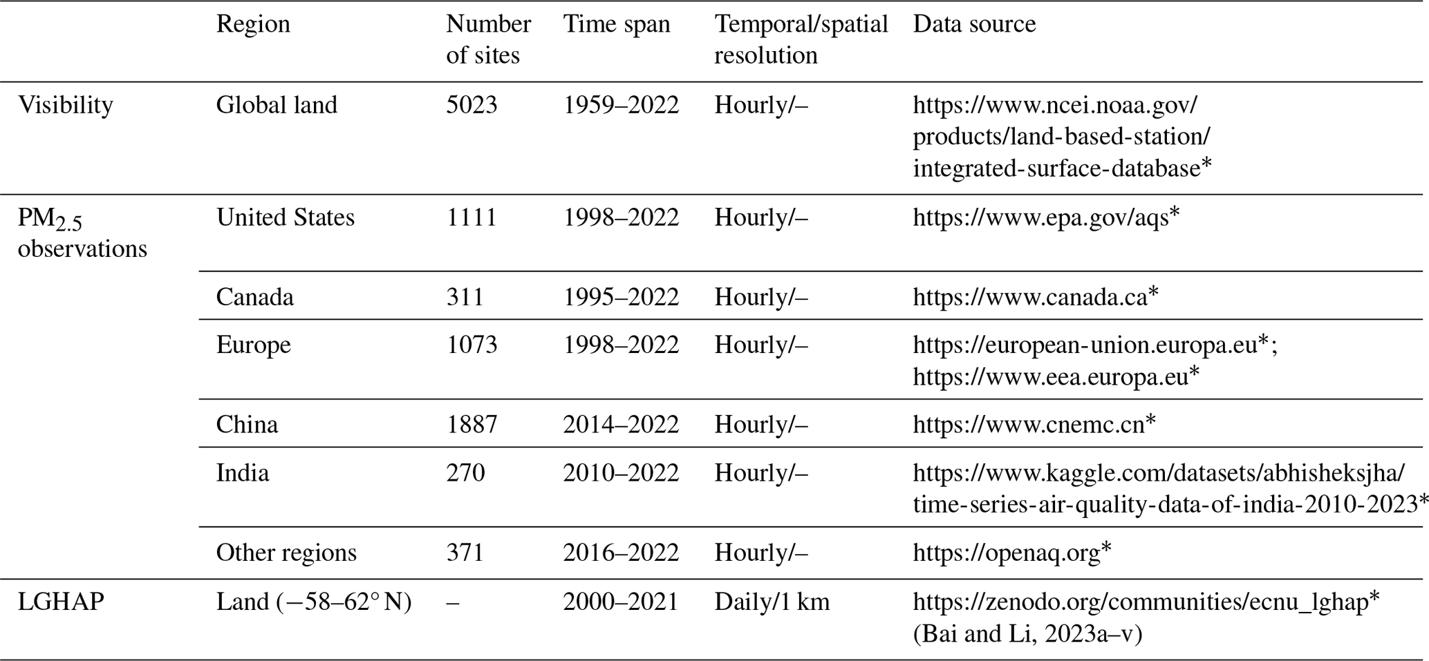
The study area is the Northern Hemisphere. Figure 1 shows the distributions of visibility stations (a) and the PM_2.5 monitoring sites (b). Table 1 lists information of stations such as the number and time span in each region. The number of visibility stations and PM_2.5 monitoring sites is 5023. Due to the establishment of a PM_2.5 monitoring network related to national or regional development, the record length and distribution of PM_2.5 observation are uneven. In this study, the site-scale PM_2.5 observations are met in at least 3 years. These sites are densely populated in North America, east and south Asia, and Europe and are very sparse in regions such as Africa, South America, and west Asia.

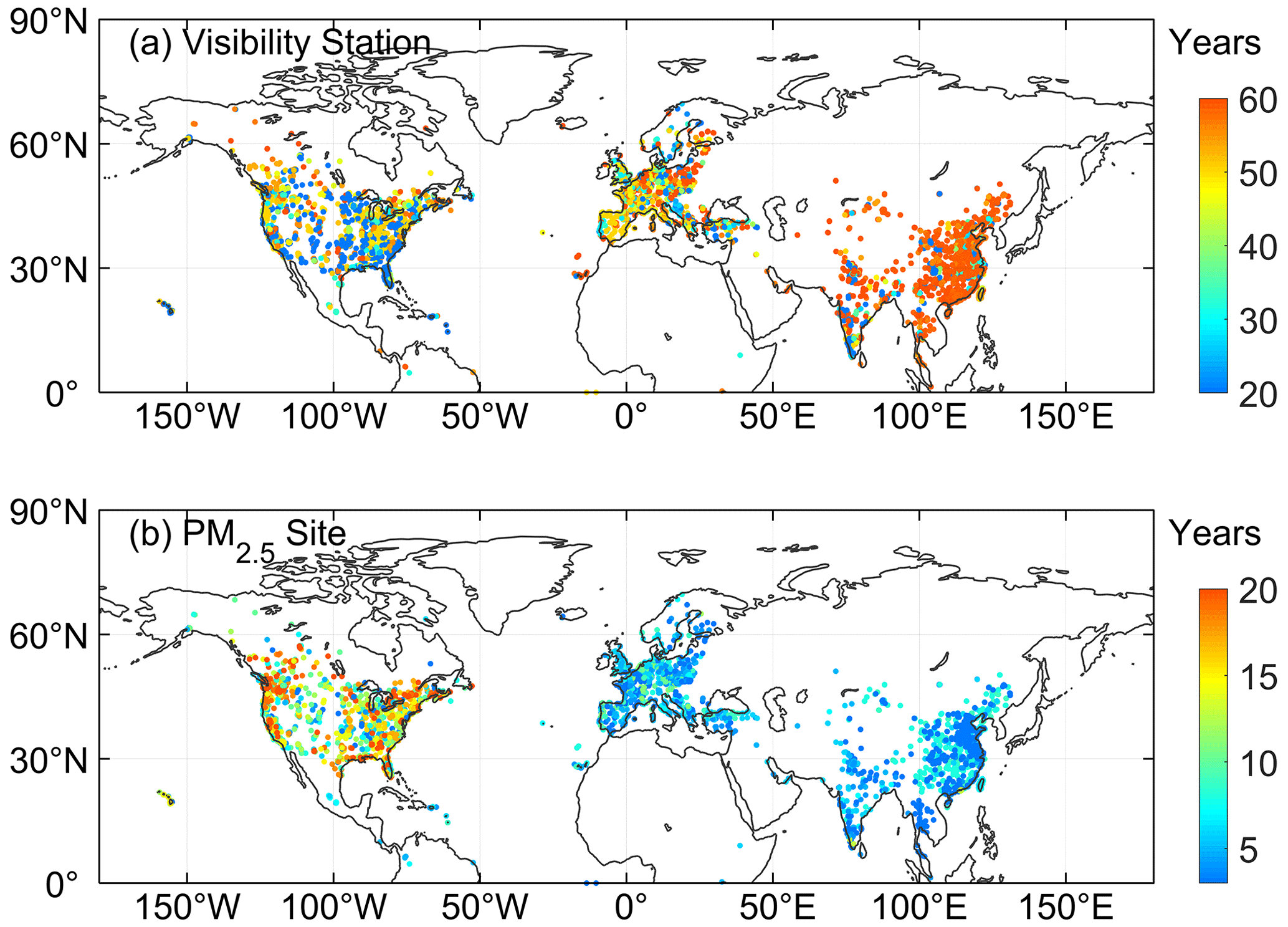
Figure 1 Study area and distributions of visibility stations (a) and PM_2.5 monitoring sites (b). The color of marker (circle) represents the year number of visibility observations and PM_2.5 concentration observations.

Table 1 Data summary.

^* Last access: 30 August 2024.

2.2 PM_2.5 data

2.2.1 PM_2.5 data in the United States

The hourly PM_2.5 concentration data for the United States from 1998 to 2022 are sourced from the Air Quality System (AQS) and are available at https://www.epa.gov/aqs (last access: 30 August 2024). The AQS provides PM_2.5 mass monitoring and routine chemical speciation data and contains other ambient air pollution data collected by the U.S. Environmental Protection Agency (EPA) and state, local, and tribal air pollution control agencies from thousands of monitors, comprising the federal reference method (FRM) and the federal equivalent method (FEM). The primary purpose of both methods is to assess compliance with the PM_2.5 National Ambient Air Quality Standards (NAAQS). FRMs include in-stack particulate filtration, and FEMs include beta-attenuation monitoring, very sharply cut cyclones, and tapered element oscillating microbalances (TEOMs). The measurement precision is ± (1–2) µg m⁻³ (hour) (Hall and Gilliam, 2016). The TEOM and beta attenuation are automatic and near-real-time monitoring methods. The TEOM, which is based on gravity, measures the mass of particles collected on filters by monitoring the frequency changes in tapered elements. The beta-attenuation method uses beta-ray attenuation and particle mass to measure the PM_2.5 concentration. In this study, we use two PM_2.5 measurement methods, FRM/FEM (88101) and non-FRM/FEM (88502). The 88502 monitors are “FRM-like” but are not used for regulatory purposes. Both the 88101 and 88502 monitors are used for reporting daily air quality index values.

2.2.2 PM_2.5 data in Canada

The hourly PM_2.5 concentration data for Canada from 1995 to 2022 are sourced from the National Air Pollution Surveillance (NAPS) program and are available at https://www.canada.ca (last access: 30 August 2024). The NAPS program is a collaborative effort between Environment and Climate Change Canada and provincial, territorial, and regional governments and is the primary source of environmental air quality data. Since 1984, PM_2.5 concentrations have been measured in Canada using a dichotomous sampler. Continuous or real-time particle monitoring began in the NAPS network in 1995 using TEOMs and beta-attenuation monitoring (Demerjian, 2000). The samples are supplemented by U.S. EPA (FRM) samples obtained after 2009 (Dabek-Zlotorzynska et al., 2011).

2.2.3 PM_2.5 data in Europe

The hourly PM_2.5 concentration data for Europe from 1998 to 2012 are obtained from the AirBase database, which is available at https://european-union.europa.eu (last access: 30 August 2024). The hourly PM_2.5 concentration data (E1a) from 2013 to 2022 are obtained from the AirQuality database, which is available at https://www.eea.europa.eu (last access: 30 August 2024). AirBase is maintained by the European Environment Agency (EEA) through its European Topic Center on Air Pollution and Climate Change Mitigation. AirBase contains air quality monitoring data and information submitted by participating countries throughout Europe. After the Air Quality Directive 2008/50/EC was enforced, the PM_2.5 concentration data began to be stored in the AirQuality database. The main monitoring methods for PM_2.5 concentration include TEOMs and beta attenuation (Green and Fuller, 2006; Chow et al., 2008). The sites are distributed across rural, rural–near city, rural–regional, rural–remote, suburban, and urban areas.

2.2.4 PM_2.5 data in China

The hourly PM_2.5 concentration data for China from 2014 to 2022 are obtained from the China National Environmental Monitoring Center and are available at https://www.cnemc.cn (last access: 30 August 2024). The continuous monitoring of PM_2.5 nationwide began in 2013, and PM_2.5 concentration data are available to the public (Su et al., 2022). There were about 2000 air quality observation sites in 2022. PM_2.5 concentrations are measured using the TEOM and beta-attenuation method (S. Zhao et al., 2016; Miao and Liu, 2019). According to the China Environmental Protection Standards, instrument maintenance, data transmission, data assurance, and quality control ensure the reliability of PM_2.5 concentration measurements. The uncertainty in the PM_2.5 concentration is <5 µg m⁻³ (Pui et al., 2014).

2.2.5 PM_2.5 data in India

The hourly PM_2.5 concentration data for India from 2010 to 2022 are obtained from the Central Pollution Control Board (CPCB) and are available at https://www.kaggle.com/datasets/abhisheksjha/time-series-air-quality-data-of-india-2010-2023 (last access: 30 August 2024). The Air Prevention and Control of Pollution Act of 1981 is enacted by the Central Pollution Control Board (CPCB) of the Ministry of Environment, Forest and Climate Change (MoEFCC). The National Air Quality Monitoring Programme (NQAMP) is a key air quality monitoring program employed by the government of India that is managed by the CPCB in coordination with the State Pollution Control Boards (SPCBs) and UT Pollution Control Committees (PCCs). A standard of 60 µg m⁻³ PM_2.5 concentration over 24 h was added in 2009. The methods used by the Indian National Ambient Air Quality Standards (NAAQS) for PM_2.5 concentration and related component measurements include the FRM and FEM (Pant et al., 2019). The measurement precision is ± (1–2) µg m⁻³ (hour).

2.2.6 PM_2.5 data in other regions

The hourly PM_2.5 concentration data of other regions from 2016 to 2022 are from OpenAQ (https://openaq.org, last access: 30 August 2024), which is a nonprofit organization providing air quality data. These air quality data are collected from environmental protection departments and other departments around the world without any processing; therefore they have good accuracy. The PM_2.5 concentrations are usually measured by the TEOM and beta-attenuation method and have been used for scientific research (Jin et al., 2022; Tan et al., 2022).

2.3 Visibility and meteorological data

The hourly visibility and meteorological data are from the Integrated Surface Database (ISD) (Smith et al., 2011), which is a global database that consists of hourly and synoptic surface observations and is archived at the NOAA's National Centers for Environmental Information (NCEI), available at https://www.ncei.noaa.gov/products/land-based-station/integrated-surface-database (last access: 30 August 2024). The ISD integrates data from more than 100 original data sources, incorporates data from over 35 000 stations around the world, and includes observation data dating back to 1901. The strict quality control algorithms are used to ensure data quality by checking data format, extreme values and limits, consistency between parameters, and continuity between observations. Detailed information about the quality control is available at http://www.ncei.noaa.gov/pub/data/inventories/ish-qc.pdf (last access: 30 August 2024). The best spatial coverage of stations is evident in North America, Europe, Australia, and parts of Asia, and the coverage in the Northern Hemisphere is better than the Southern Hemisphere.

Visibility and meteorological records are filtered by the geophysical report type code. The codes FM-12 and FM-15 are selected. The FM-12 code represents the report being from the Surface Synoptic Observations (SYNOP) report, which is a coding system developed by the World Meteorological Organization (WMO) for reporting observation data from ground meteorological stations. The FM-15 code represents the report being from the Meteorological Terminal Aviation Routine Weather Report (METAR), providing weather information at the airport and its surrounding areas. The format and content of the METAR are consistent globally and comply with WMO's international meteorological observation and reporting standards. The frequency of the SYNOP report is generally every 3 or 6 h, and the frequency of the METAR is usually once per hour.

In this study, visibility is an essential variable for PM_2.5 concentration. The reciprocal of visibility is directly proportional to the aerosol extinction coefficient, which is closely related to the PM_2.5 concentration (Wang et al., 2009, 2012). Considering that temperature, wind speed, humidity, and precipitation are factors that impact particle dispersion, particle growth, and secondary generation (Zhang et al., 2020), temperature, dew point temperature, wind speed, and precipitation are selected.

2.4 Data preprocessing

When processing the visibility and meteorological variables, we use some screening conditions from previous studies (Husar et al., 2000; Wang et al., 2009; Li et al., 2016; Zhong et al., 2021). We remove the records with missing visibility, temperature, dew point temperature, wind speed, and hourly precipitation greater than 0.1 mm. Relative humidity is calculated using the Goff–Gratch formula (Goff, 1957). When relative humidity is greater than 90 %, the record is removed to reduce the influence of fog, even precipitation. In high-latitude regions, the low-visibility records caused by ice fog and snow are removed when the temperature is less than −29 °C and the wind speed is greater than 16 km h⁻¹. Since PM_2.5 exhibits hygroscopic growth, dry visibility is calculated when relative humidity is between 30 % and 90 % (Yang et al., 2021).

$$\begin{array}{}\text{(1)}& \mathrm{VISD}=\mathrm{VIS}/(\mathrm{026}+\mathrm{04285}\times \log \left(\mathrm{100}-\mathrm{RH}\right)),\end{array}$$

where VIS is the visibility, RH is the relative humidity, and VISD is the dry visibility.

For a single visibility site, there should be at least five non-repetitive visibility values and at least three valid records per day. The upper limit of visibility is set to the 99 % percentile of visibility (Li et al., 2016). The harmonic mean is used to calculate the daily VIS and VISD because it can better capture rapid weather changes and enhance daily representativeness. The arithmetic mean is used for other variables.

The maximum hourly PM_2.5 concentration is set to 1000 µg m⁻³. The daily PM_2.5 concentration needs at least 3-hourly records. We select the PM_2.5 monitoring sites with a condition of at least 3-year continuous monitoring. The distribution of PM_2.5 sites is shown in Fig. 1, and the details are shown in Table 1.

The spatial matching between the PM_2.5 site and visibility station adopts the nearest principle, and the upper limit of distance is set to 100 km. Experiments show that the upper limit of distance has little effect on model training and prediction, but when the upper limit is small, the number of site pairs significantly decreases, especially in Asia. Matched visibility stations are not used again. To match more PM_2.5 monitoring sites, we construct a “virtual” visibility station, whose variables are established by the average of variables of the two nearest visibility stations.

We merge daily PM_2.5 concentration and visibility and other meteorological variables. We have adopted two matching methods: (1) merge at the hourly scale first and then calculate the daily mean, and (2) calculate the daily mean first and then match them. The results of two methods have no impact on the training of the model, but there are differences in the predicted results. Since SNOPY's visibility is not continuously observed hourly, we select the second method to merge PM_2.5 concentration and visibility data on the daily scale to improve the daily representativeness of estimated PM_2.5 concentration.

2.5 PM_2.5 data for comparison

The Long-term Gap-free High-resolution air Pollutants (LGHAP) dataset provides daily PM_2.5 concentrations from 2000 to 2021 over global land, with a 1 km grid resolution, and is available at https://zenodo.org/communities/ecnu_lghap (last access: 30 August 2024). The PM_2.5 concentration is estimated using aerosol optical depth and other factors such as geographic location, land cover type, climate zone, and population density, based on a deep learning approach, termed the scene-aware ensemble learning graph attention network. The correlation coefficient with ground-based measurements is 0.95, and the RMSE is 5.7 µg m⁻³ (Bai et al., 2024). This dataset provides global PM_2.5 concentration with a high spatiotemporal resolution.

For most regions in the Northern Hemisphere, except for North America and Europe, the duration of continuous monitoring PM_2.5 concentration data is relatively short, making it difficult to evaluate historical PM_2.5 concentration. For example, the PM_2.5 monitoring network in China was implemented from the end of 2012, resulting in the inability to verify the PM_2.5 concentrations before 2012. Therefore, we compare our data with the LGHAP PM_2.5 concentration to evaluate the predictive ability of the model and the consistency of our data on the temporal scale.

2.6 Decision tree regression

We employ decision tree regression (Teixeira, 2004) to estimate daily PM_2.5 concentrations. The key to decision tree regression is to find the optimal split variable and optimal split point. The optimal split point of the predictor is determined by the minimum mean square error, which determines the optimal tree structure. Decision tree regression is a commonly used nonlinear machine learning method that partitions the feature space based on the mapping between feature attributes and response values, with each leaf node representing a specific output for each feature space region. Its ability to handle complex relationships with relatively few model parameters is advantageous, minimizing the risk of overfitting and enabling the prediction of continuous and categorical predictive variables.

The sample data include the predictor and response. The predictor is composed of nine variables: the reciprocal of dry visibility (Vis_Dry_In), the reciprocal of visibility (Vis_In), temperature (Temp), dew point temperature (Td), temperature−dew point difference (Temp-Td), relative humidity (RH), wind speed (WS), wind numerical time (DateTime), and daily record number (DailyObsNum). Both visibility and meteorological variables are daily means. The response variable is the daily monitored PM_2.5 concentration.

For each site, we sort the sample data by time, with the first 80 % being the training set and the last 20 % being the test set. Due to the inconsistent sample length among different sites, this approach is appropriate for sites with small sample sizes (such as only 3-year observations). We use a 10-fold cross-validation method (Browne, 2000) to train the model. The test set is used to evaluate the predictive ability of the model.

2.7 Evaluation metrics

2.7.1 Statistical metrics

We use the root mean square error (RMSE), mean absolute error (MAE), and correlation coefficient (ρ) as evaluation metrics to evaluate the model's performance and predictive ability. The formulas are given as follows:

$$\begin{array}{}\text{(2)}& {\displaystyle }\mathrm{MSE}=\sqrt{{\displaystyle \frac{\mathrm{1}}{n}}{\sum }_{i=\mathrm{1}}^n{\left(y_i-{\widehat{y}}_i\right)}^{\mathrm{2}}}\text{(3)}& {\displaystyle }\mathrm{MAE}={\displaystyle \frac{\mathrm{1}}{n}}{\sum }_{i=\mathrm{1}}^n\left|y_i-{\widehat{y}}_i\right|\text{(4)}& {\displaystyle }\mathit{\rho }={\displaystyle \frac{{\sum }_{i=\mathrm{1}}^n(y_i-\stackrel{\mathrm{‾}}{y})({\widehat{y}}_i-\stackrel{\mathrm{‾}}{\widehat{y}})}{\mathrm{sqrt}\left({\sum }_{i=\mathrm{1}}^n(y_i-\stackrel{\mathrm{‾}}{y}{)}^{\mathrm{2}}{\sum }_{i=\mathrm{1}}^n({\widehat{y}}_i-\stackrel{\mathrm{‾}}{\widehat{y}}{)}^{\mathrm{2}}\right)}},\end{array}$$

where y_i and $\stackrel{\mathrm{‾}}{y}$ are the predicted value and the average of the predicted values; ${\widehat{y}}_i$ and $\stackrel{\mathrm{‾}}{\widehat{y}}$ are the target and the average of the target; and $i=\mathrm{1},\mathrm{2},\mathrm{\dots },n$, where n is the length of the sample.

2.7.2 Partial dependence

The importance of predictor variables is assessed via partial dependence. Partial dependence represents the relationship between the individual predictive variable and the predicted response (Friedman, 2001). By marginalizing the other variables, the expected response of the predicted variable is calculated. All the partial dependences of the predicted response on the subset of predicted variables are calculated. The calculation process of the partial dependency method is described next.

The dataset of the predictor is X, $X=[X^{\mathrm{1}},X^{\mathrm{2}},\mathrm{\dots },X^n]$, and n represents the number of predictive factors. The complement of subset X^s is X^c, where X^s is a single variable in X, and X^c is all other variables in X. The predicted response f(x) depends on all variables in X, and it is expressed as follows:

$$\begin{array}{}\text{(5)}& f\left(x\right)=f(X^{\mathrm{s}},X^{\mathrm{c}}).\end{array}$$

The partial dependence of the predicted response to X^s is expressed as follows:

$$\begin{array}{}\text{(6)}& f^{\mathrm{s}}\left(X^{\mathrm{s}}\right)=\int f\left(X^{\mathrm{s}},X^{\mathrm{c}}\right)\mathrm{pC}\left(X^{\mathrm{c}}\right)\mathrm{d}{X}^{\mathrm{c}},\end{array}$$

where pC(X^c) is the marginal probability of X^c; that is, $\mathrm{pC}\left(X^{\mathrm{c}}\right)\approx \int f\left(X^{\mathrm{s}},X^{\mathrm{c}}\right)\mathrm{d}{X}^{\mathrm{s}}$. Assuming that the likelihood of each observation is equal, the dependence between X^s and X^c and the interactions of X^s and X^c in the response are not strong. The partial dependence is shown as

$$\begin{array}{}\text{(7)}& f^{\mathrm{s}}\left(X^{\mathrm{s}}\right)\approx {\displaystyle \frac{\mathrm{1}}{N}}{\sum }_{i=\mathrm{1}}^{N}f\left(X^{\mathrm{s}},X_i^{\mathrm{s}}\right),\end{array}$$

where N is the number of observations, and i represents the ith observation.

2.7.3 Generalized additive mixed model

The generalized additive mixed model (GAMM) originates from two independent yet complementary statistical methods: the generalized additive model (GAM) and mixed-effects models. GAM was introduced by Trevor Hastie and Robert Tibshirani in the 1980s (Hastie and Tibshirani, 1987). GAM employs smooth functions (such as splines) to replace linear terms in traditional regression, capturing nonlinear relationships between response and explanatory variables. The primary aim of GAM is to enhance model flexibility, allowing the data to determine the form of the nonlinear relationships rather than pre-specifying them. The mixed-effects model includes both fixed and random effects, enabling the analysis of hierarchical and correlated data (Verbeke and Lesaffre, 1996). Fixed effects apply to the entire sample, whereas random effects account for variations within individuals or groups, explaining data correlation and variability. GAMM represents the evolution of statistical models from linear to nonlinear, from simple to complex, and from single effects to mixed effects. GAMM has been widely applied in various fields, such as ecology, climate, and air pollution, becoming an essential tool for studying complex nonlinear relationships and hierarchical data (Park et al., 2013; Polansky and Robbins, 2013; Chang et al., 2017; Ravindra et al., 2019).

The relationship between PM_2.5 concentrations and time (e.g., months, seasons) is typically nonlinear and exhibits seasonal variation. GAMM uses smooth functions (such as splines) to capture the nonlinear variations and model the periodic features with cyclical smooth functions. Interannual variations in PM_2.5 concentrations can also be captured using smooth functions. Due to the inherent autocorrelation in time series, GAMM effectively handles the autocorrelation by incorporating time-related smooth functions or random effects, thereby enhancing the model accuracy. PM_2.5 concentrations from neighboring locations often exhibit spatial correlation. GAMM can address this spatial correlation by introducing spatially correlated smooth functions or random effects. Therefore, it is also suitable for spatial variations, especially when the spatial distribution of site observations is uneven.

Based on the GAMM, the PM_2.5 concentration y(i,t) at site i and time t can be expressed as

$$\begin{array}{}\text{(8)}& y(i,t)=\mathit{x}\mathit{\beta }+f(\cdot )+b(i,t)+\mathit{\epsilon }(i,t).\end{array}$$

The following is an explanation of the expression and parameter settings.

Linear terms. xβ includes the terms of site elevation and the overall mean PM_2.5 concentration, where x is the vector of explanatory variables, and β is a coefficient vector.

Smooth terms. f(⋅) can be decomposed into three individual smooth terms, i.e., the seasonal smooth term, interannual smooth term, and spatial smooth term, as shown in Eq. (9).

$$\begin{array}{}\text{(9)}& f(\cdot )=f\left(\mathrm{month}\right)+f\left(\mathrm{year}\right)+f\left(\mathrm{spatial}\right)\end{array}$$

They are composed of linear combinations using spline basis functions. The seasonal smooth term is a function of the month. The smooth function is the penalized regression cyclic cubic splines (assumed with periodic nature) (Wood et al., 2016), and the knot number is 12. The interannual smooth term is a function of year. The smooth function is the penalized regression cubic splines (Wood et al., 2016), and the knot number is 64. The spatial smooth term is a function of longitude and latitude. The smooth function is the Gaussian-process-penalized regression splines (Kammann and Wand, 2003), and the knot number is 80. In this study, they are used to describe the regional long-term PM_2.5 concentration annual cycle, interannual trends, and spatial distribution, respectively.

The term of station-specific effects, b(i,t), is a random effect term to describe the differences between observation sites, based on the assumption that observations are independent.

The residual noise term ε(i,t) is a first-order autoregressive term.

More explanations about GAMM are detailed in the R package mgcv. Some studies also provide an introduction and selection of parameters (Polansky and Robbins, 2013; Chang et al., 2017; Ravindra et al., 2019).

3 Results and discussion

3.1 Evaluation of variable importance

We evaluate the contribution of each variable to the response by partial dependence. The variable with the highest partial dependence value is the most important variable in the model. Figure 2a shows the proportion of the most important variables for all sites, and Fig. 2b shows the ranking of the importance of all variables. The reciprocal of dry visibility is the most important variable at 65.8 % of sites, and the reciprocal of visibility is the second-most-important variable at 14.9 % of sites. The contribution of meteorological variables ranges from 2.1 % to 6.6 %. The time variable contributes 1.7 %. The lowest contribution is the daily number of visibility record at only 0.9 % because it is only a variable that describes the daily representativeness of visibility. It also indicates that daily visibility has high daily representativeness (under the conditions of at least 3-hourly records).

The PM_2.5 concentration level varies spatially, which is related to regional geographical environment, climate, and air quality laws and regulations. Therefore, we analyze the importance of variables in different regions, as shown in Fig. 2c–h. The two most important variables are still reciprocal of dry visibility and reciprocal of visibility, with a proportion of 73.1 % in the United States, 77.5 % in Canada, 80.8 % in Europe, 98.8 % in China, and 60.2 % in India. It indicates that PM_2.5 concentration is the most significantly correlated with visibility in China. The contribution of meteorological variables is significantly higher in the United States and India than in other regions. It indicates that meteorological conditions have a significant contribution to PM_2.5 concentration in these regions, which may be related to the formation mechanism and transport of particulate matter.

The above results indicate a strong correlation between the PM_2.5 concentration and visibility, as visibility can be considered an indicator of air quality without fog or precipitation. Meteorological factors play secondary roles, which influence the formation, dispersion, and deposition of PM_2.5 (Gui et al., 2020; Zhong et al., 2022). Although the number of daily records and the time have the most negligible impacts on the PM_2.5 concentration in the model, they have significant impacts on the cyclical changes and daily representativeness of PM_2.5 concentration (Wang et al., 2012; Zhang et al., 2020).

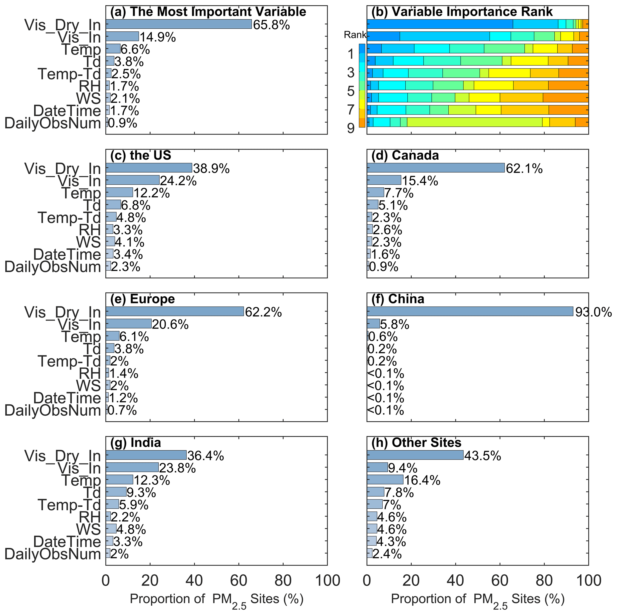
Figure 2 The most important variable (a) and the ranking (b) at all sites. The most important variable in each region (c–h). The stacked bar shows the importance rankings of the variables (“rank = 1” represents the most important variable). The bar shows the proportion of the most important variable. The variables are the reciprocal of dry visibility (Vis_Dry_In), reciprocal of visibility (Vis_In), temperature (Temp), dew point temperature (Td), temperature−dew point difference (Temp-Td), relative humidity (RH), wind speed (WS), numerical time (DateTime), and daily number of visibility record (DailyObsNum).

3.2 Evaluation of model performance

We analyze the linear regression relationship between all estimated and corresponding response values to evaluate the model's performance. Figure 3 is the density scatter plot of the monitored PM_2.5 concentration (response values) and the estimated PM_2.5 concentration (estimated values). There is a total of 8 031 473 data pairs for all the sites. The linear regression slope (95 % confidence interval) is 0.955 [0.955, 0.955], the R² is 0.95, the RMSE is 7.2 µg m⁻³, and the MAE is 3.2 µg m⁻³.

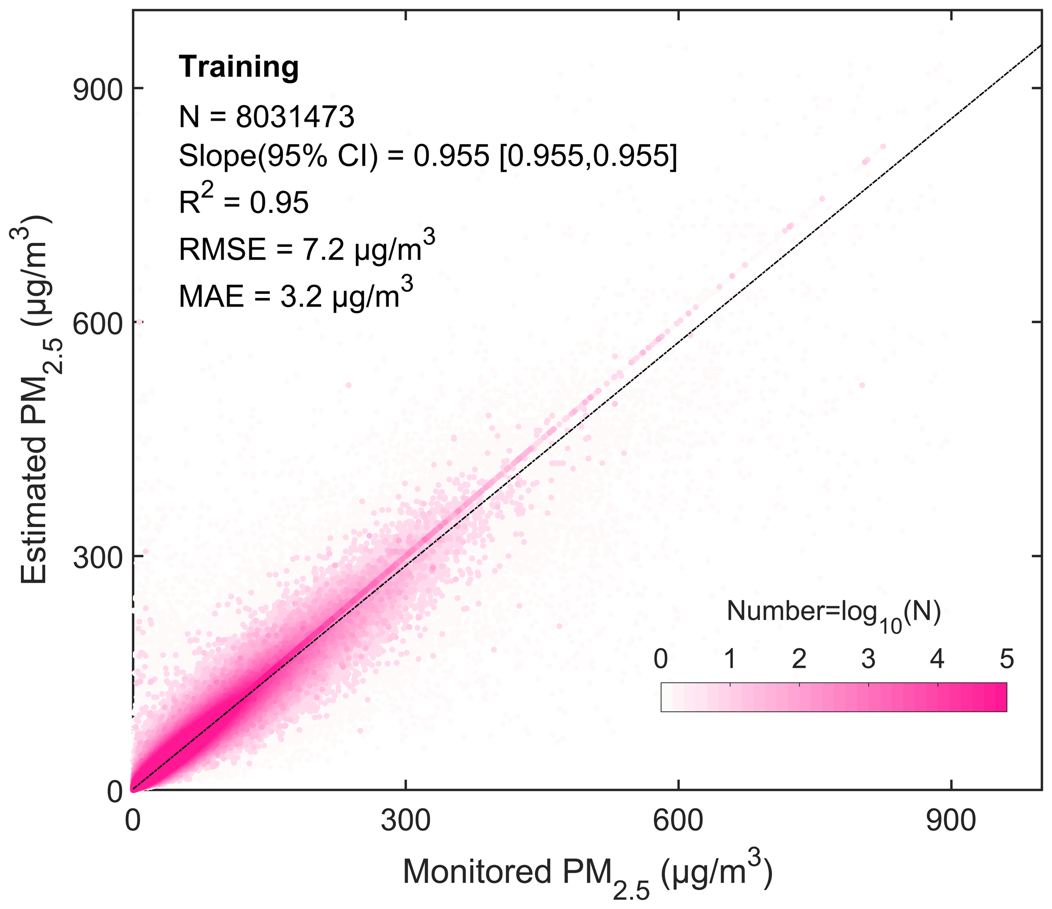
Figure 3 Density scatter plot (a) between estimated PM_2.5 concentration and monitored PM_2.5 concentration. The dashed black line is the linear regression line. N is the length of the data pairs, and slope is the linear regression coefficient within a 95 % confidence interval (CI). R² is the coefficient of determination, RMSE is the root mean square error, and MAE is the mean absolute error.

Figure 4a–c show the spatial distribution (a–c) and frequency of training of RMSE, MAE, and ρ. Table 2 lists the model's performance metrics in the United States, Canada, Europe, China, and India. For all sites, the average RMSE is 6.92 µg m⁻³, with a median of 4.76 µg m⁻³. The RMSE of 80 % of the sites is less than 10.01 µg m⁻³. The RRMSE (the ratio of RMSE to the mean of PM_2.5 concentration) is 28.7 %. The MAE is 3.77 µg m⁻³, with a median of 2.72 µg m⁻³. The MAE is less than 5.66 µg m⁻³ for 80 % of the sites. The RMAE (the ratio of MAE to the mean of the PM_2.5 concentration) is 15.4 %. The average ρ is 0.91, and the median is 0.92. The ρ of 80 % of the sites is greater than 0.87. Previous studies have shown that for PM_2.5 concentration retrieved from daily visibility or satellite aerosol optical depth, the R² range of the model is from 0.42 to 0.89, and the RMSE range is from 9.59 to 32.09 µg m⁻³ (Shen et al., 2016; Liu et al., 2017; Wei et al., 2019b; Gui et al., 2020; Li et al., 2021; Zhong et al., 2021). This finding indicates that our model performs well at the daily scale.

On the regional scale, the RMSE values for the United States, Canada, Europe, China, and India are 3.10, 2.78, 4.92, 9.65, and 17.46 µg m⁻³, respectively, and the RRMSE values are 34.9 %, 40.4 %, 29.8 %, 23.1 %, and 28.8 %, respectively. The MAEs for the United States, Canada, Europe, China, and India are 1.61, 1.35, 2.54, 5.47, and 9.13 µg m⁻³, respectively. The RMAEs are 17.9 %, 19.5 %, 16.3 %, 13.1 %, and 14.4 %, respectively. The ρ values for the United States, Canada, Europe, China, and India are 0.87, 0.88, 0.91, 0.94, and 0.92, respectively. The correlation coefficients are higher in China and India and lower in the United States and Canada.

The largest RMSE and MAE are in India, and the smallest are in Canada. The RRMSE and RMAE are larger in the United States, Canada, and Europe than in China and India and other regions.

Table 2 The metrics for all sites and sites in the United States, Canada, Europe, China, and India. RRMSE is the ratio of the RMSE to the mean of PM_2.5 concentration (in %). RMAE is the ratio of the MAE to the mean of PM_2.5 concentration.

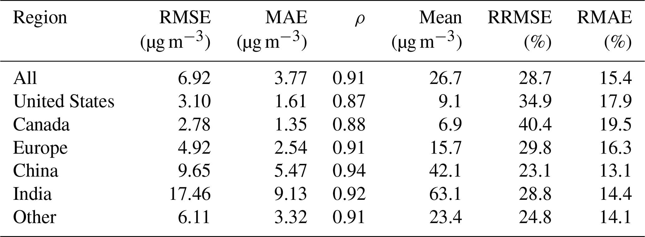
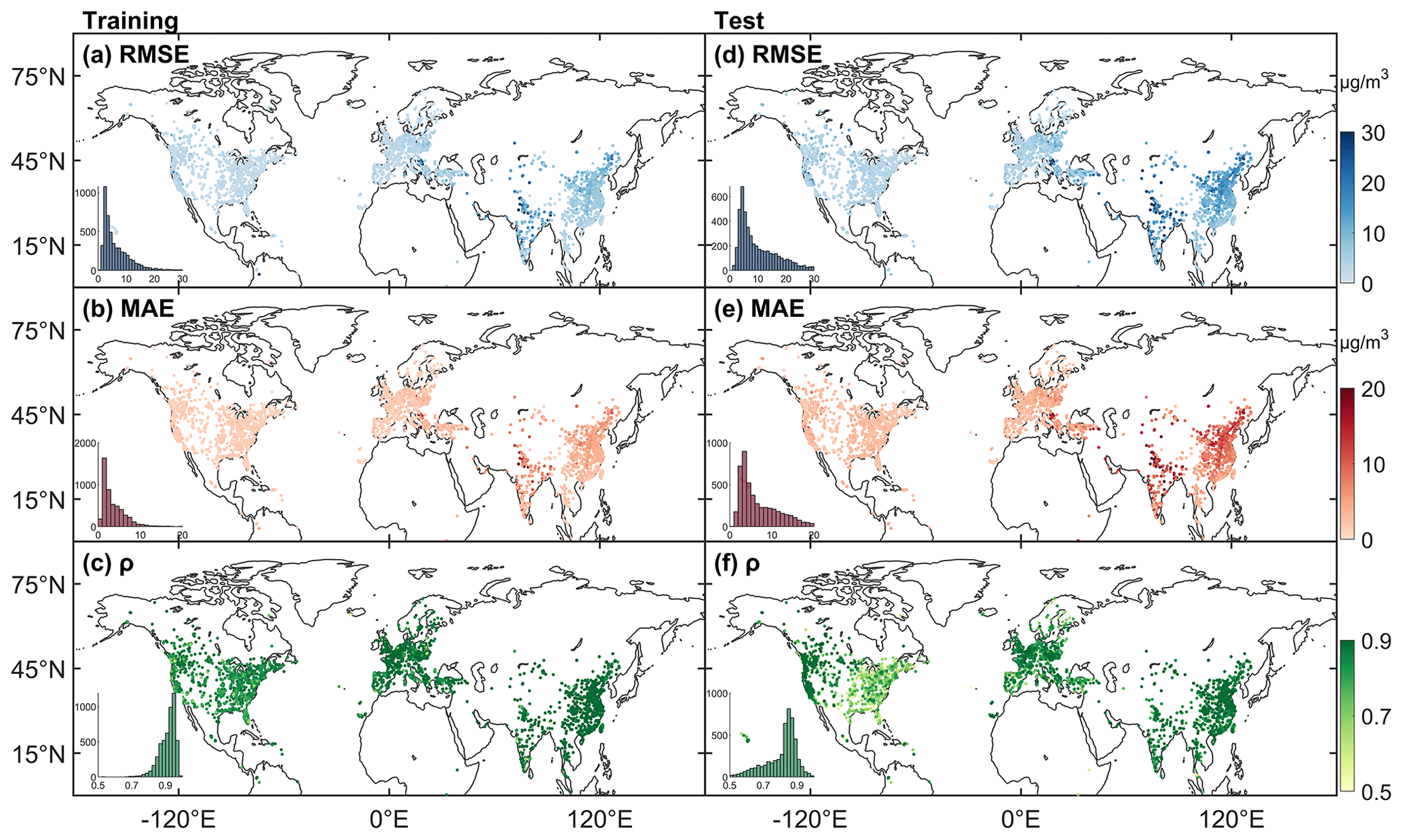
Figure 4 Statistical metrics' distribution of training (a, b, c) and test (d, e, f) data. The bar is the frequency of sites. RMSE is the root mean square error, MAE is the mean absolute error, and ρ is the correlation coefficient.

3.3 Evaluation of model's predictive ability

A total of 1 911 183 pairs of test data are employed to evaluate the model's predictive ability. Figure 5 is the density scatter plot between the predicted PM_2.5 concentration and the test PM_2.5 concentration. The linear regression slope (95 % CI) is 0.864 [0.863, 0.865], R² is 0.79, RMSE is 14.8 µg m⁻³, and MAE is 7.6 µg m⁻³. Previous studies have shown that the R² range of the model's predictive results at the daily scale is 0.31–0.84, and the RMSE range is 13.8–29.0 µg m⁻³ (Gui et al., 2020; Zhong et al., 2021). The test results exhibit excellent predictive capability.

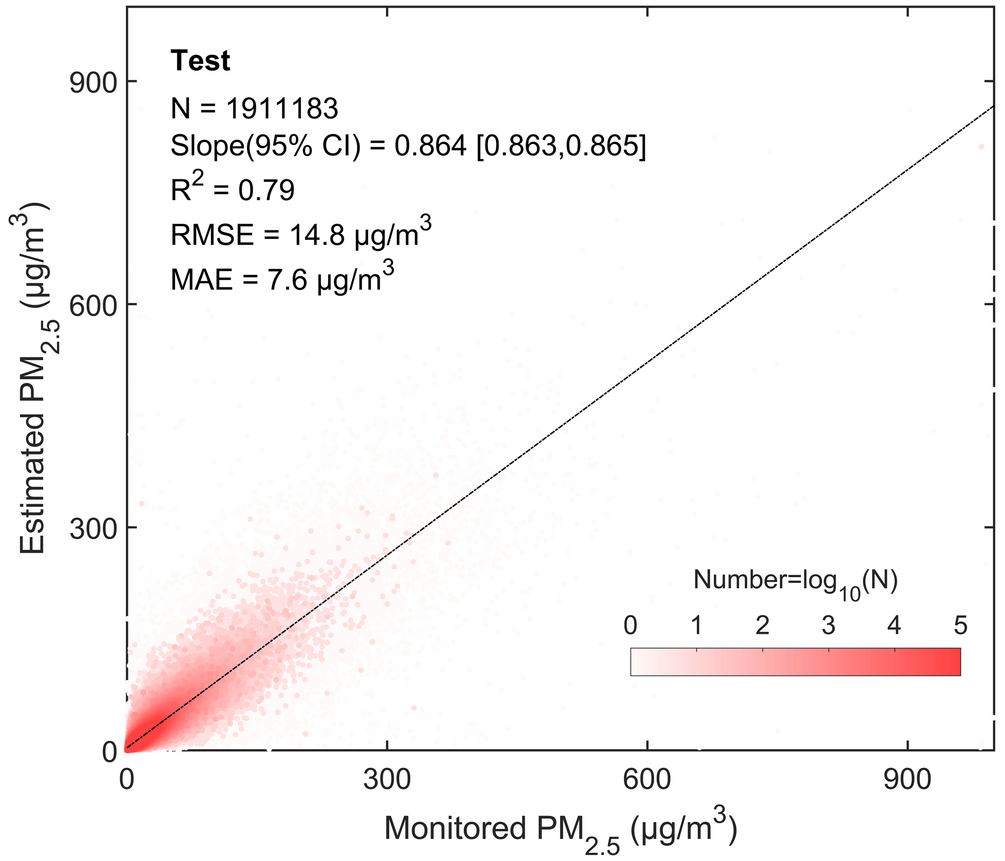
Figure 5 Density scatter plot (a) between the predicted PM_2.5 concentration and monitored PM_2.5 concentration of the test results. The dashed black line is the linear regression line. N is the length of the data pairs, and slope is the linear regression coefficient within a 95 % confidence interval (CI). R² is the coefficient of determination, RMSE is the root mean square error, and MAE is the mean absolute error.

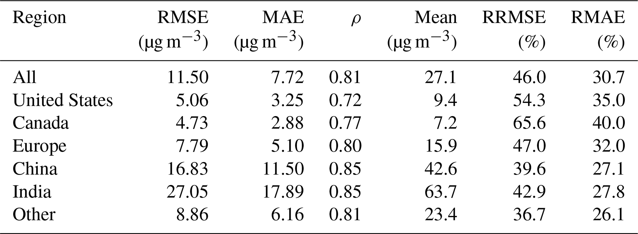
We analyze the test results for Canada, the United States, Europe, China, and India to assess the predictive ability of the model in different regions. Figure 4d–f show the spatial distributions of the test RMSE, MAE, and ρ and their frequency. Table 3 lists the test results of the metrics. For all sites, the average RMSE is 11.50 µg m⁻³. The RRMSE is 46.0 %. The average MAE is 7.72 µg m⁻³. The RMAE is 30.7 %. The ρ is 0.81. For the United States, the RMSE, MAE, and ρ are 5.06, 3.25 µg m⁻³, and 0.72, respectively. For Canada, the RMSE, MAE, and ρ are 4.73, 2.88 µg m⁻³, and 0.77, respectively. The results in the United States and Canada are better in the west than in the east. The RMSE, MAE, and ρ for Europe are 7.79, 5.10 µg m⁻³, and 0.80, respectively. For China, the RMSE, MAE, and ρ are 16.83, 11.50 µg m⁻³, and 0.85, respectively. For India, the RMSE, MAE, and ρ are 27.05, 17.89 µg m⁻³, and 0.85, respectively. The results show that in developing regions (China and India), ρ is better than that in developed regions (the United States, Canada, and Europe), which means that the predictive ability of the model is better for severely polluted regions.

Table 3 The test results of the model's performance metrics for all sites and sites in the United States, Canada, Europe, China, and India. RRMSE is the ratio of the RMSE to the mean of PM_2.5 concentration (in %). RMAE is the ratio of the MAE to the mean of PM_2.5 concentration (in %).

3.4 Uncertainties and limitations

3.4.1 Uncertainty in the pollution level

Figure 6 shows the uncertainty in the predicted PM_2.5 concentration with respect to the pollution level of the monitored PM_2.5 concentration. For all sites, the uncertainty in the bias increases as the pollution level increases. The mean and median of the bias shift from positive to negative with increasing pollution levels; 83.6 % of PM_2.5 concentration data is less than 45 µg m⁻³, and the mean bias (<0.8 µg m⁻³) is positive; 36.8 % is less than 10 µg m⁻³, and the median (<0.4 µg m⁻³) of the bias is positive; 16.4 % of PM_2.5 concentration is greater than 45 µg m⁻³, and the mean bias is negative; and 63.2 % of PM_2.5 concentration is greater than 10 µg m⁻³, and the median is negative. It indicates that the model overestimates at low pollution levels and underestimates at high pollution levels.

The bias for each region also increases with pollution level. For the United States, the mean bias of 69.4 % is positive and less than 0.8 µg m⁻³, and the PM_2.5 concentration is less than 10 µg m⁻³. When the PM_2.5 concentration is greater than 10 µg m⁻³, the mean bias is negative. For Canada, the mean bias of 74.1 % is positive and less than 0.7 µg m⁻³. When the PM_2.5 concentration is greater than 8 µg m⁻³, the mean bias is negative. For Europe, the mean bias of 67.1 % is positive and less than 0.9 µg m⁻³. When the PM_2.5 concentration is greater than 15 µg m⁻³, the mean bias is negative. For China, 67.7 % of the bias is positive and less than 2.7 µg m⁻³. When the PM_2.5 concentration is greater than 45 µg m⁻³, the mean bias is negative. For India, 80.1 % of the bias is positive and less than 4.2 µg m⁻³, and when the PM_2.5 concentration is greater than 100 µg m⁻³, the mean bias is negative. When the PM_2.5 concentration is greater than 60 µg m⁻³, the bias median is negative, with a percentage of 40.3 %. The uncertainty in each region is similar, and the uncertainty increases as the pollution level increases.

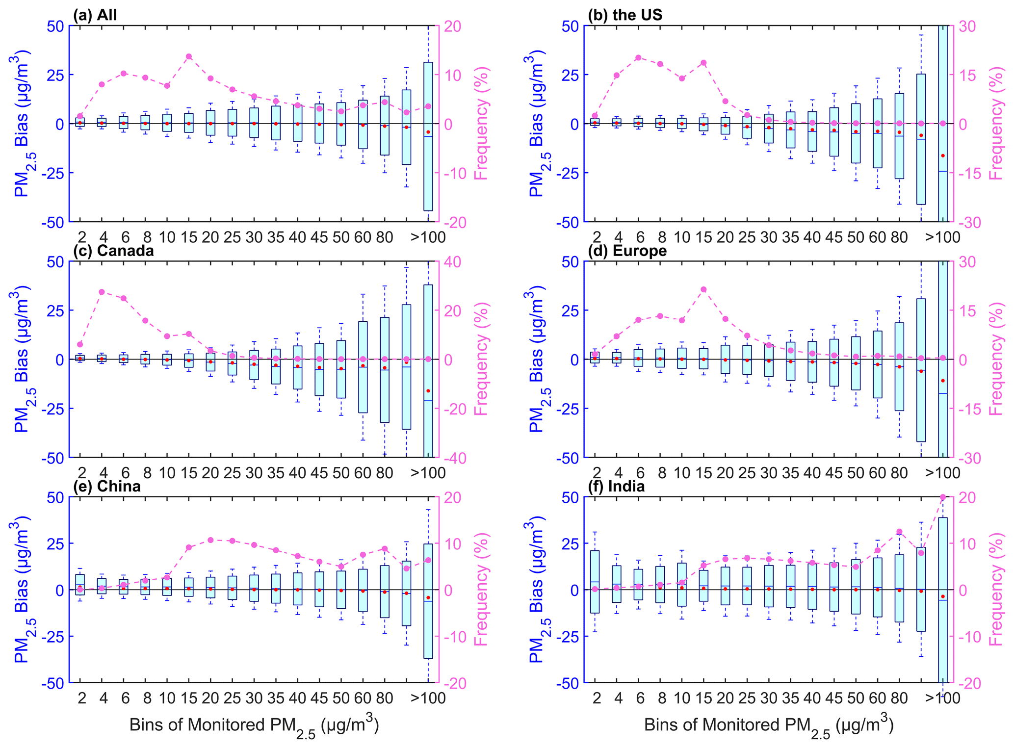
Figure 6 Box plots of the pollution level and bias (predicted PM_2.5 concentration – monitored PM_2.5 concentration) for all sites (a) and sites in the United States (b), Canada (c), Europe (d), China (e), and India (f). The box's upper and lower limits represent ±1 standard deviation, the whiskers represent 2 times the standard deviation, the red circle represents the median, and the short line represents the mean bias. The frequency (%) on the right-hand y axis represents the percentage of data with different pollution levels (dashed line).

3.4.2 Uncertainty in the station elevation

With the spatial variability in PM_2.5 concentration, we analyze the mean bias at different visibility station elevations. Figure 7 shows the relationships between the elevations of the visibility stations and the bias. The bias exhibits variations across different elevations for all stations. The mean bias of all sites ranges from −0.04 to 0.02 µg m⁻³. A total of 90.1 % of the stations have positive biases. The median of the bias is almost positive, with a positive bias of 99.5 % stations, except for the elevation at 4 km. The elevations of 86.5 % of the stations are less than 1 km, with a positive median of the bias. High uncertainties in bias occur at elevations of 0.05, 0.2, and 0.3 km. Negative biases are observed at elevations of 0.4, 0.9–1, and 4 km. This finding indicates a nonsignificant overestimation of the predicted PM_2.5 concentration due to the various elevations.

The bias patterns vary across regions. For the United States, a total of 88.8 % of the stations have negative biases. The median of the bias is negative with a percentage of 63.4 %. High uncertainties in bias occur at elevations of 0.05, 2, and 0.3 km. For Canada, 52.3 % of the stations have positive biases. The median of the bias is negative with a percentage of 33.8 %. High uncertainties in bias occur at elevations of 0.05 and 1 km. For Europe, 58.9 % of the stations have positive biases. The median of the bias is negative with a percentage of 40.2 %. High uncertainties in bias occur at elevations of 0.05 and 0.9 km. For China, 76.7 % of the stations have negative biases. The median of the bias is negative with a percentage of 54.1 %. High uncertainties in bias occur at elevations of 0.05, 0.5, and 3 km. For India, 68.1 % of the stations have positive biases. The median of the bias is negative with a percentage of 63.8 %. The elevation of most stations with a high uncertainty is at 0.05 km. High uncertainties in bias occur at elevations of 0.1 and 3 km. More stations with negative bias are in the United States and China. More stations with positive bias are in Canada, Europe, and India.

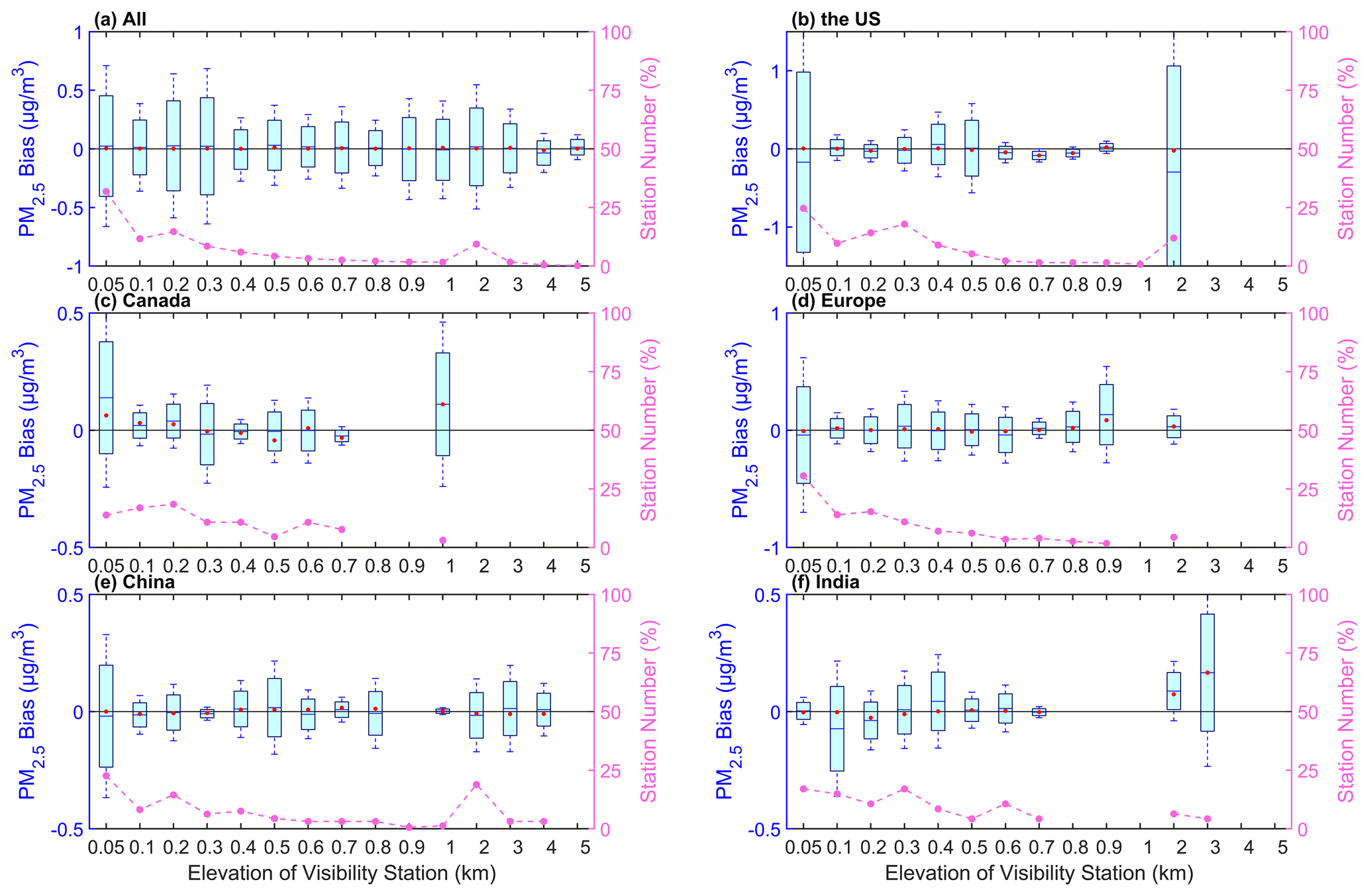
Figure 7 Box plots of the bias (predicted PM_2.5 concentration–monitored PM_2.5 concentration) and the elevation of the visibility station for all sites (a) and sites in the United States (b), Canada (c), Europe (d), China (e), and India (f). The box's upper and lower limits represent ±1 standard deviation, the whiskers represent 2 times the standard deviation, the red circle represents the median, and the short line represents the mean bias. The station number (%) on the right-hand y axis represents the percentage of the station number at different elevations (dashed line).

3.4.3 Uncertainty in the station distance

As the visibility stations and PM_2.5 sites are not collocated, we analyze the mean bias of PM_2.5 concentration at different distances, as shown in Fig. 8. For all sites, 86.1 % of the stations have negative biases. The median of the bias is negative with a percentage of 70.8 %. More stations have a negative bias caused by the distance. The uncertainty has no signification with the distance. The distances with low uncertainties are at 1 and 20–40 km. The distances with high uncertainties are at 5 and 60 km.

For the United States, 63.1 % of the stations have negative biases. The median of the bias is negative with a percentage of 69.2 %. The distance with the lowest uncertainty is at 1 km. The distances with high uncertainties are at 5 and 60 km. For Canada, 60.0 % of the stations have positive biases. The median of the bias is positive with a percentage of 80.0 %. The uncertainty shows an increase with the distance increasing. For Europe, 72.7 % of the stations have negative biases. The median of the bias is positive with a percentage of 67.1 %. When the distance is less than 10 km, the uncertainty increases with the distance. The distances with low uncertainties are at 1 and 30–40 km. The distances with high uncertainties are at 10 and 75 km. For China, 64.3 % of the stations have negative biases. The median of the bias is negative with a percentage of 72.7 %. The distance with a low uncertainty is at 30 km. The distance with a high uncertainty is at 60 km. For India, 62.3 % of the stations have negative biases. The median of the bias is positive with a percentage of 59.1 %. The distance with the lowest uncertainty is at 30 km. The distance with the highest uncertainty is at 20 km.

More visibility stations have negative biases, except for the stations in Canada. For the stations in the United States, Canada, and Europe, the lowest uncertainty is at 1 km. For the stations in China and India, the uncertainty has no significant relationship with distance, though the distance has caused a negative bias.

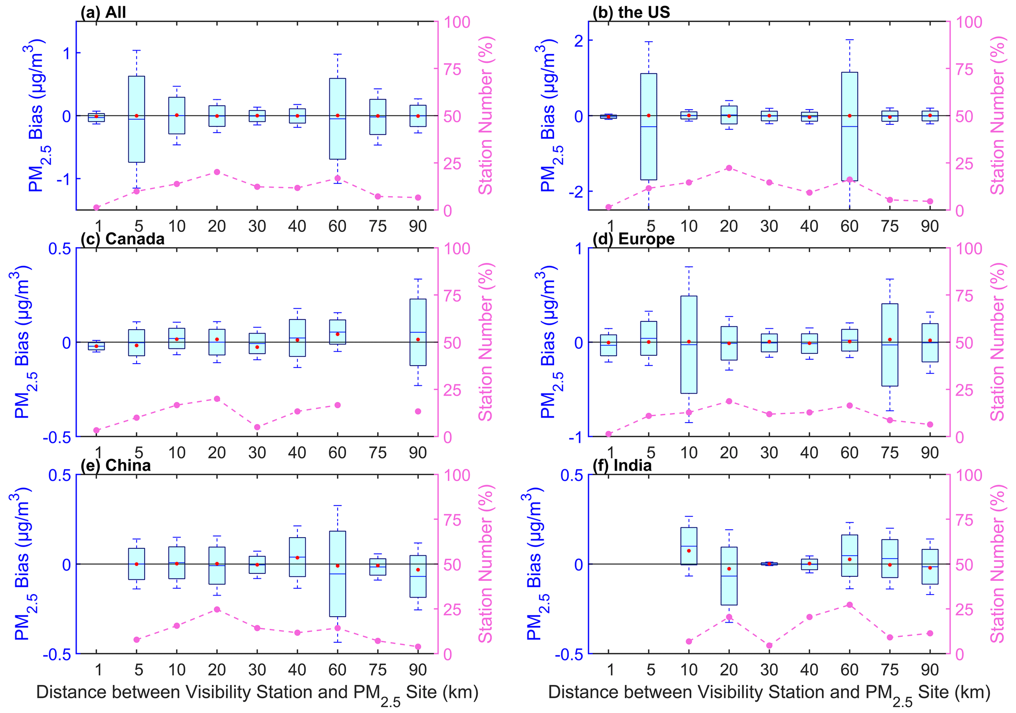
Figure 8 Box plots of the mean bias (predicted PM_2.5 concentration–monitored PM_2.5 concentration) and the distance between the visibility station and the PM_2.5 site and for all sites (a) and sites in the United States (b), Canada (c), Europe (d), China (e), and India (f). The box's upper and lower limits represent ±1 standard deviation, the whiskers represent 2 times the standard deviation, the red circle represents the median, and the short line represents the mean bias. The station number (%) on the right-hand y axis represents the percentage of the station number at different distances (dashed line).

3.4.4 Discussion on the uncertainties and limitations

There are some uncertainties and limitations in this study. The upper limit of visibility and PM_2.5 concentration can cause some uncertainties in model training. The maximum distance between the visibility stations and PM_2.5 monitoring sites is 100 km due to the spatial variability in aerosols, which may increase the uncertainty in the estimated PM_2.5 concentration. Because of the nonuniform vertical distribution of aerosols, the different elevations of the visibility stations and the PM_2.5 monitoring sites further increase the uncertainty in estimating PM_2.5 concentration. In addition, the spatial coverage of visibility stations, especially in China and India, is still limited, which may increase the uncertainty in the representativeness of regional PM_2.5 concentration and pollution levels. With the increasing human concern of air pollution and the implementation of air pollution control measures, the types of major atmospheric pollutants may have changed at regional scale, the composition of particulate matter has also evolved, the scattering and absorption characteristics may have changed, and the relationship between visibility and PM_2.5 concentration may change. These changes may lead to uncertainties in estimating historical PM_2.5 concentration. It is challenging to validate data using ground observations and satellite-based estimation prior to 2000. Despite these limitations and challenges, we establish a long-term PM_2.5 concentration dataset based on visibility from 1959 to 2022, which has been carefully validated and evaluated, providing insights into the long-term spatiotemporal characteristics of concentration PM_2.5 in the Northern Hemisphere.

4 Comparisons with other PM_2.5 concentration datasets

We compare the daily and monthly estimated PM_2.5 concentration with the LGHAP PM_2.5 concentration from 2000 to 2021 to further demonstrate the reliability the estimated PM_2.5 concentration. When comparing on the regional scale, we split the time range into 2000–2010 and 2011–2021 to further validate the accuracy and consistency of estimated PM_2.5 concentrations, as in some regions such as India and China, there are almost no continuous PM_2.5 monitoring data before 2010.

4.1 Comparisons on the daily scale

We spatiotemporally match the LGHAP PM_2.5 concentration with the estimated PM_2.5 concentration. Figure 9 shows the density scatter plot between the estimated PM_2.5 concentration and LGHAP PM_2.5 concentration. There is a total of 96 188 682 pairs during the period of 2000 and 2021, 46 846 389 pairs during the period from 2000 to 2010, and 49 342 302 during the period of 2011 and 2021, with slopes of 0.817, 0.758, and 0.867. The intercepts are 6.928, 8.933, and 5.377 µg m⁻³, respectively. The slope decreases before 2010, which may be related to the upper limit of LGHAP PM_2.5 concentration with a significantly decreasing quantity of the concentration (>300 µg m⁻³).

We further compare the PM_2.5 concentrations of the annual calendar cycles on the regional scale in Fig. 10. The PM_2.5 concentration of each day is the mean of the PM_2.5 concentrations at all sites in the region. The correlation coefficients of the PM_2.5 concentrations are greater than 0.89 from 2011 to 2021 and greater than 0.92 from 2000 to 2010. The correlation is greater in Europe, China, and India than in the United States and Canada. There is no significant difference in the variation of annual calendar cycles between two periods on the regional scale. In the United States, PM_2.5 concentration between 2000 and 2010 is more similar than the concentration between 2011 and 2021, and the bias decreases. In Canada, the correlation coefficient increases, although the bias increases. In Europe, the correlation coefficient and bias increase. There are similar changes in China and India. The bias increases on days 1 to 60 and 300 to 366, but the correlation remains significant. The difference of PM_2.5 concentration during the two periods is mainly reflected in the increasing bias in Canada and Europe, which is a non-seasonal bias, and the increasing bias in winter in China and India, which is a seasonal bias. Overall, PM_2.5 concentrations show a good consistency before and after 2010 on the daily scale.

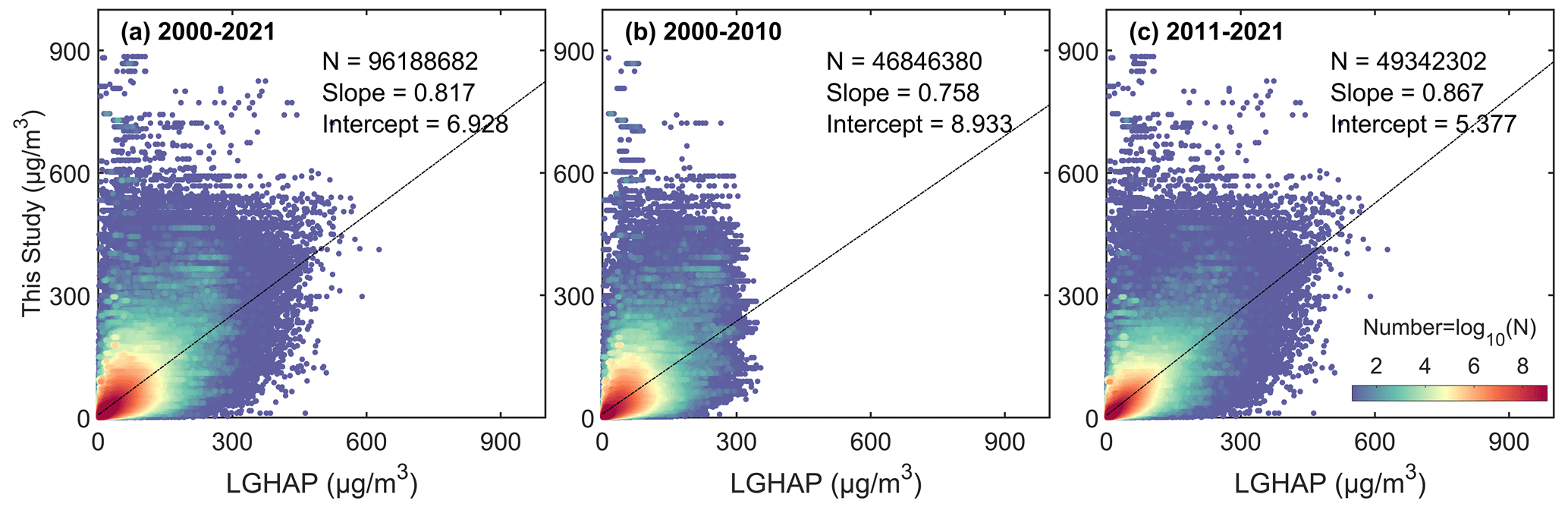
Figure 9 Density scatter plot between the estimated PM_2.5 concentration (this study) and LGHAP PM_2.5 concentration on the daily scale from 2000 to 2021 (a), from 2000 to 2010 (b), and from 2011 to 2021 (c). The dashed black line is the linear regression line. N is the length of the data pairs, and slope is the linear regression coefficient. Intercept represents the y intercept.

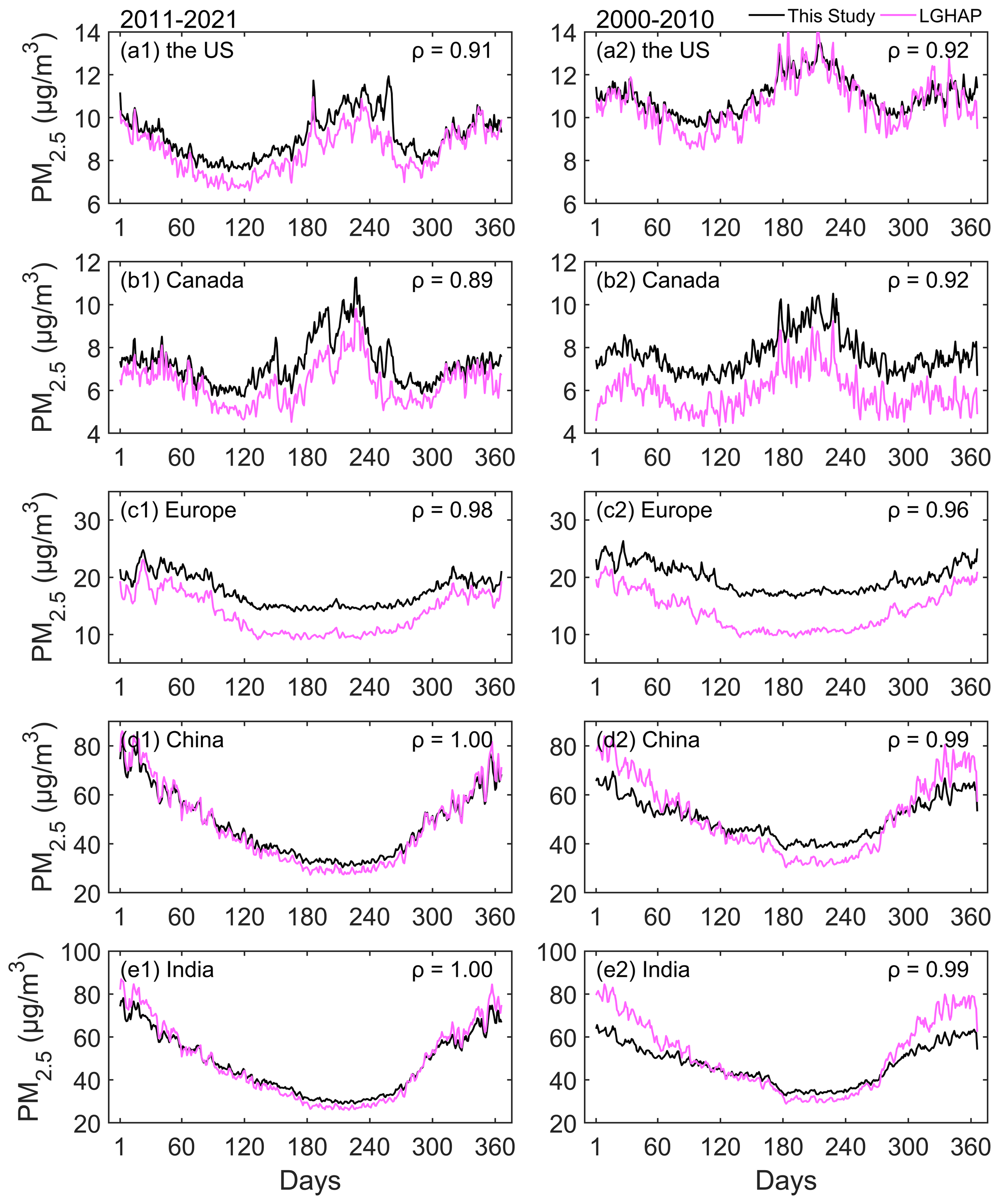
Figure 10 Comparison of annual calendar cycle of PM_2.5 concentration on the regional scale from 2011 to 2021 (left) and from 2000 to 2010 (right) between the estimated PM_2.5 concentration (this study) and LGHAP PM_2.5 concentration on the daily scale. ρ is the correlation coefficient.

4.2 Comparisons on the monthly scale

Figure 11 shows the density scatter plot between the estimated PM_2.5 concentration and LGHAP PM_2.5 concentration on the monthly scale. The monthly PM_2.5 concentration is calculated by the matched daily concentrations. There is a total of 3 296 739 pairs during the period from 2000 to 2021, 1 582 161 pairs during the period from 2000 to 2010, and 1 714 578 during the period from 2011 to 2021, with slopes of 0.857, 0.821 and 0.879. The intercepts are 6.774, 8.716, and 5.272 µg m⁻³, respectively. The slope of monthly concentration significantly improves before 2010 and slightly increases after 2010 compared to the daily scale.

We also compare the PM_2.5 concentrations of the annual cycles on the regional scale in Fig. 12. The PM_2.5 concentration of each month is the mean of the PM_2.5 concentrations at all sites in the region. The correlation coefficients of the PM_2.5 concentrations are greater than 0.92 from 2011 to 2021 and greater than 0.87 from 2000 to 2010. In the United States, the PM_2.5 concentrations before 2010 are closer compared to those after 2010, except in April and August, and the biases in other months have significantly decreased. In Europe and Canada, the biases have increased. In China, the result is similar to the result on the daily scale. In India, the performance of the two is almost consistent, with a correlation coefficient of 0.99 and 0.96. The two datasets have a very high similarity in annual cycles, indicating that the estimated PM_2.5 concentration in this study is accurate and consistent before and after 2010.

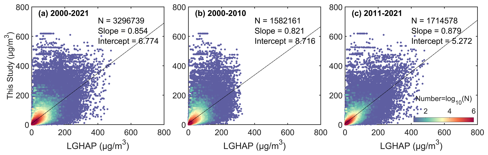
Figure 11 Density scatter plot between the estimated PM_2.5 concentration (this study) and LGHAP PM_2.5 concentration on the monthly scale from 2000 to 2021 (a), from 2000 to 2010 (b), and from 2011 to 2021 (c). The dashed black line is the linear regression line. N is the length of the data pairs, and slope is the linear regression coefficient. Intercept represents the y intercept.

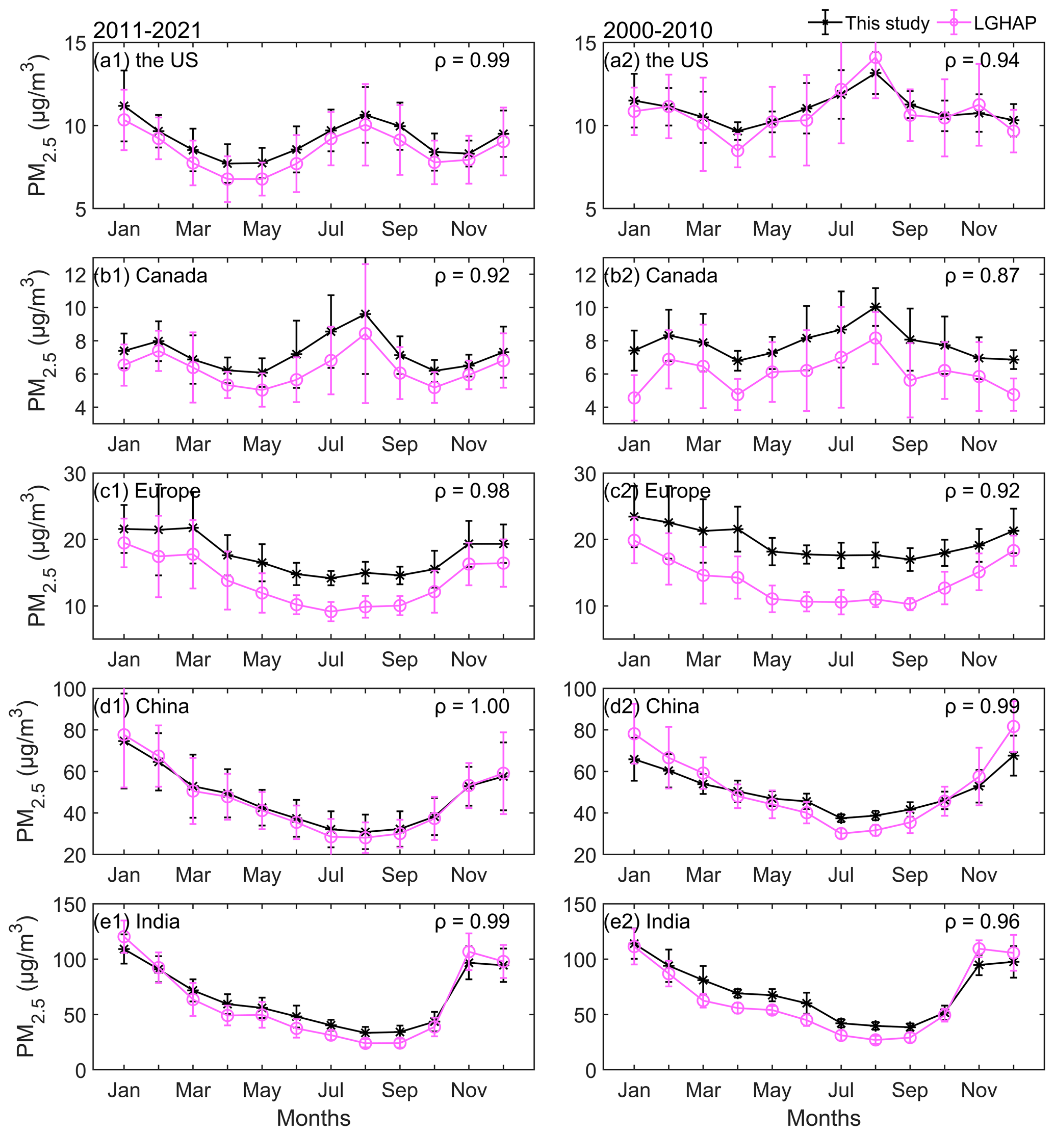
Figure 12 Comparison of annual cycle of monthly PM_2.5 concentration on the regional scale from 2011 to 2021 (left) and from 2000 to 2010 (right) between the estimated PM_2.5 concentration (this study) and LGHAP PM_2.5 concentration on the daily scale. ρ is the correlation coefficient.

4.3 Discussion on the differences of PM_2.5 concentration estimated using visibility and aerosol optical depth

Both visibility and aerosol optical depth are excellent alternatives for estimating PM_2.5 concentration, with its own advantages. However, they have differences in principle, which may be the reason for the difference between the two datasets in comparison.

Fine particulate matter near the ground surface affects atmospheric visibility through scattering. Studies have shown visibility has a negative correlation with PM_2.5 concentration, and the reciprocal of visibility has a positive correlation with the extinction coefficient and has a negative correlation with the particulate matter concentration (Wang et al., 2012; Zhang et al., 2017, 2020). Therefore, visibility is often used as a proxy for particulate matter pollution (Huang et al., 2009; Singh et al., 2020), and it is the basis for estimating PM_2.5 concentration. In addition, studies have shown that meteorological observations such as temperature and humidity also play an important role in estimating PM_2.5 concentration using visibility (Shen et al., 2016; Xue et al., 2019; Zhong et al., 2021). Therefore, when estimating PM_2.5 concentration based on visibility data, only conventional meteorological variables need to be added, which is convenient and accurate observational data. In addition, the long-term, complete, and highly temporal ground-based observations are the advantages of historical estimation of PM_2.5 concentration. The daily mean from continuous or equidistant hourly observations greatly increases the daily representativeness.

The aerosol optical depth is a physical quantity that describes aerosol column properties. It is the integration of the extinction coefficient in the vertical direction. When establishing a connection between aerosol optical depth and near-ground PM_2.5 concentration, it is essential to consider the vertical structure of aerosols. Studies have shown that the aerosol vertical profiles usually are provided by observations, assumptions, or chemical transport models to obtain the aerosol properties near the surface (Van Donkelaar et al., 2010; Wei et al., 2019b; Van Donkelaar et al., 2021). Van Donkelaar et al. (2006, 2010) have demonstrated that aerosol vertical profile errors in chemical transport models and aerosol optical depth retrieval and sampling result in an approximately 25 % uncertainty of 1 standard deviation. Sensitivity testing shows that a 1 % estimation error in the aerosol optical depth can lead to a 0.27 % estimation error in the PM_2.5 concentration (Wei et al., 2021). In addition, the retrieval of aerosol optical depth is affected by clouds or surface types and a finite number of daily observations (usually one to two times), though it has the advantage of high spatial coverage (Liu et al., 2017; Singh et al., 2020; Zhong et al., 2021).

Another difference is the upper limit of PM_2.5 concentration. In this study, the upper limit of the estimated daily PM_2.5 concentration is set to 1000 µg m⁻³ (the same for input data). When the PM_2.5 concentration is greater than 500 µg m⁻³ during heavy pollution, which may contribute to the higher frequency at high pollution levels than in the LGHAP dataset, especially before 2010. We do not remove visibility records during dust weather when preprocessing the data, which may lead to an overestimation of PM_2.5 concentration in dusty areas, such as northern China and northwestern India. In Sect. 3.4, the uncertainty analysis has provided an explanation for the overestimation. Overall, our PM_2.5 concentration dataset has a good consistency with PM_2.5 concentration based on aerosol optical depth.

5 Regional trends and spatial patterns

We use the estimated PM_2.5 concentrations (at least 10 d records in a site) to calculate monthly PM_2.5 concentrations and analyze the annual cycles, interannual trends, and spatial patterns of PM_2.5 concentrations in different regions based on the GAMM. The annual variation comes from the monthly smooth term of GAMM, the interannual variation comes from the annual smooth term, and the spatial pattern comes from the spatial smooth term. The regions include Canada, the United States, Europe, China, and India. The results are shown in Fig. 13. The trend from 1959 to 2022 in each region is the slope of the Theil–Sen (ST slope) estimators (Sen, 1968; Theil, 1992), and the Mann–Kendall test (Mann, 1945; Kendall, 1948) is used to calculate the significance of the trend. The test results show that the p values are all less than 0.01 in all regions.

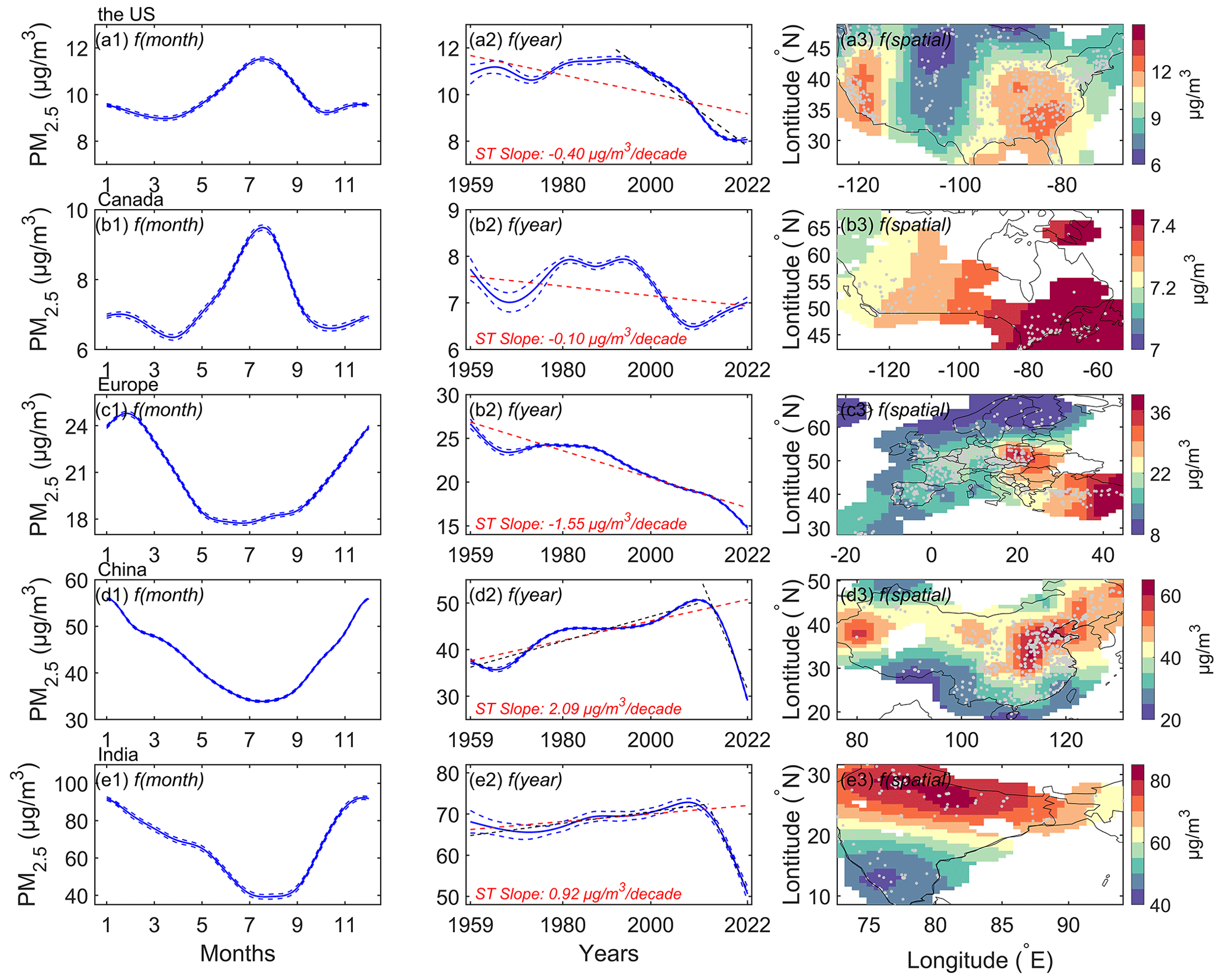
Figure 13 Annual cycles, interannual trends, and spatial patterns of PM_2.5 concentrations in the United States (a1–a3), Canada (b1–b3), Europe (c1–c3), China (d1–d3), and India (e1–e3). The left column “f(month)” is the annual cycle, the middle column “f(year)” is the interannual trend, and the right column “f(spatial)” is the spatial distribution from the generalized additive mixed model (GAMM). The dashed blue lines represent ±1 standard error of the month and annual mean of PM_2.5 concentrations. The dashed red or black lines represent the trends of the Theil–Sen estimators (ST slope). The Mann–Kendall test of trends shows that the p values are less than 0.01 in all regions. The scatter points in right column are the locations of PM_2.5 monitoring sites.

In the United States, the annual cycle curve shows that the PM_2.5 concentration is a “double peak and double valley” shape. The peaks occur in July and December, respectively, with the highest PM_2.5 concentration in July throughout the year. The valley values are in April and October, and the PM_2.5 concentration levels are equivalent. The trend is −0.40 µg m⁻³ per decade, and PM_2.5 concentration decreases significantly after 1992, with a trend of −1.39 µg m⁻³ per decade. The areas of high PM_2.5 concentration are in the east and west. The areas with low PM_2.5 concentrations are mainly located in the central and northern regions. The high concentration in the eastern and western regions is related to extensive industrial activities and densely populated cities. The low concentration in the central and northern regions is related to high vegetation coverage, low industrial activity, and low population density.

In Canada, the annual cycle curve also shows that the PM_2.5 concentration is a “double peak and double valley” shape. The peak values occur in August and February, with the highest PM_2.5 concentration in August. The valley values are in April and October. The trend is −0.10 µg m⁻³ per decade, and PM_2.5 concentration increases after 2010. The PM_2.5 concentration exhibits an east–high to west–low pattern. The eastern regions, such as Ontario and Quebec, are characterized by high population density and significant industrial and transportation activities.

In Europe, the annual cycle of PM_2.5 concentration shows that the PM_2.5 concentration is the highest in February and is low from May to September. The valley values are in April and October. The trend is −1.55 µg m⁻³ per decade. High-concentration areas are distributed in eastern Europe, while low-concentration areas are in northern and western Europe. Eastern Europe exhibits more industrialization, particularly with a prevalence of traditional heavy industries and the use of coal and other high-pollution energy sources. In contrast, the energy structure in western Europe tends to favor cleaner energy sources.

In China, the annual cycle curve of PM_2.5 concentration presents a V-like shape. It indicates that high concentrations are in winter, while low concentrations are in summer. The trend is 2.09 µg m⁻³ per decade. The trend is 2.65 µg m⁻³ per decade from 1959 to 2011 and −22.23 µg m⁻³ per decade from 2012 to 2022. High-concentration areas are distributed in northern China, such as the North China Plain, northeast China, the Sichuan Basin, Taklimakan Desert, and Badain Jaran Desert. Low-concentration areas are in southern China and the northern Tian Shan. Besides dust, industrial activities and coal combustion for heating during winter are significant contributors to the PM_2.5 concentration in northern regions.

In India, the annual cycle curve of PM_2.5 concentration also presents a V-like shape. High concentrations are in winter, and low concentrations are in summer. The trend is 0.92 µg m⁻³ per decade. The trend is 1.41 µg m⁻³ per decade from 1959 to 2013 and −23.36 µg m⁻³ per decade from 2014 to 2022. Some studies have shown that the PM_2.5 concentration in India has decreased since 2014, especially in northern cities. Singh et al. (2021) found that five major cities in India show a downward trend from 2014 to 2019, with the largest decline of approximately −4.2 µg m⁻³ yr⁻¹ in New Delhi. Ravindra et al. (2024) also found that the trend in New Delhi is about −5 µg m⁻³ yr⁻¹ from 2014 to 2020. These studies have shown a faster downward trend than our study, as these PM_2.5 monitoring sites are mainly concentrated in urban areas. The PM_2.5 concentration exhibits a north–high to south–low pattern. High-concentration areas are distributed in northern India, such as the Ganges Plain and Thar Desert, because there are more industrial and densely populated areas, and the terrain leads to the retention of air pollutants. Low-concentration areas are in the Deccan Plateau.

Above all, the PM_2.5 concentrations in developed countries and regions are significantly lower than those in developing countries in the Northern Hemisphere. Regional trends are similar to those of previous studies in different periods (Van Donkelaar et al., 2010; Wang et al., 2012; Boys et al., 2014; Ma et al., 2016; Li et al., 2017; Hammer et al., 2020). The trends in PM_2.5 concentration changes in different regions are closely associated with the implementation of relevant policies. The earlier pollution control measures are taken, the earlier the decreasing trend in the PM_2.5 concentration occurs, and the lower the threat of particulate matter pollution is to humans. In 1997, the U.S. EPA classified PM_2.5 as a hazardous substance in the National Ambient Air Quality Standard, and subsequent regulations in 2006 further strengthened the source control and management of fine particulate matter (Hall and Gilliam, 2016). In 1988, the Canadian federal government enacted the Canadian Environmental Protection Act, which enhanced the regulation of PM_2.5 (Davies, 1988). The European Union introduced the Air Quality Directive in 1996, followed by multiple revisions and updates to regulate and restrict air pollutants, including PM_2.5 (Kuklinska et al., 2015). However, Europe stands out due to its early adoption of clean production practices in heavy industries since the 1970s. Since 2012, China has implemented numerous regulations and standards for PM_2.5. For instance, the Monitoring Method for Atmospheric Particulate Matter (PM_2.5) was issued in 2012, and the Chinese Ministry of Environmental Protection released the Ambient Air Quality Standards in 2013, including emission standards for PM_2.5 (B. Zhao et al., 2016). In 2009, the Indian Ministry of Environment and Forests issued the National Ambient Air Quality Standards, which include control standards for PM_2.5. In 2019, the Indian government launched the National Clean Air Programme (NCAP) to improve air quality by implementing a series of measures to reduce the emissions of PM_2.5 and other pollutants (Ganguly et al., 2020). These environmental regulations have contributed significantly to the decline of PM_2.5 concentrations. Some studies have shown that the variation of PM_2.5 concentrations is also related to several factors, such as the energy structure, urbanization process, population distribution, and vegetation coverage (Shi et al., 2018; Wu et al., 2018; Li et al., 2019; Wang et al., 2019; Lim et al., 2020; Qi et al., 2023).

6 Data availability

Daily PM_2.5 concentration data in the Northern Hemisphere from 1959 to 2022 are available at https://doi.org/10.11888/Atmos.tpdc.301127 (Hao et al., 2024).

All site-scale PM_2.5 data files are in “PM25-Daily_1959_2022. zip”. The file name includes a region name and a site number. For example, the file name, “China_1001. txt”, means that the site is in China, and the site number is 1001, which describes the daily PM_2.5 concentration at a single site and can be directly opened using a text program (such as Notepad), separated by commas. The data include four column names: “Date”, “PM25(µg/m3)”, “Longitude(degree_east)”, and “Latitude(degree_north)”. “Date” is UTC time, “PM25(µg/m3)” is the daily PM_2.5 concentration (unit: µg m⁻³), “Longitude” is the longitude that ranged from −180 to 180° E, and “Latitude” is the latitude that ranged from 0 to 90° N.

7 Conclusions

In this study, we use a machine learning method to estimate daily PM_2.5 concentration for 5023 terrestrial sites in the Northern Hemisphere from 1959 to 2022 based on daily visibility and related meteorological variables. The first 80 % of PM_2.5 concentration data in each site are used to train the model, and the last 20 % are used to test. The model's performance and predictive ability are evaluated, and a dataset of daily PM_2.5 concentration based on aerosol optical depth is used to compare and evaluate the estimated PM_2.5 concentration. We analyze the uncertainty and discuss the limitations of our dataset. Finally, the PM_2.5 concentration variation (annual calendar cycle, interannual cycle, and spatial distribution) in five regions over the past 64 years is analyzed based on GAMM. We hope our dataset will be useful for studying the atmospheric environment, human health, and climate change and provide auxiliary support for assimilation. Several key results of this study are described as follows:

• The most important variable. Visibility is the most important variable at 80.7 % of the PM_2.5 sites, as visibility can be considered an indicator of PM_2.5 concentration without fog or precipitation. Other meteorological variables play a secondary role in the model, especially temperature and dew point temperature.

• Model performance and predictive ability. The training results show that the slope between the estimated PM_2.5 concentration and the monitored PM_2.5 concentration within the 95 % confidence interval is 0.955, the R² is 0.95, the RMSE is 7.2 µg m⁻³, and the MAE is 3.2 µg m⁻³. The test results show that the slope between the predicted PM_2.5 concentration and the monitored PM_2.5 concentration is 0.864 ±0.0010 within a 95 % confidence interval, R² is 0.79, RMSE is 14.8 µg m⁻³, and MAE is 7.6 µg m⁻³. The model shows good stability and predictive ability. Compared with a global PM_2.5 concentration dataset based on satellite retrieval, the slopes of linear regression on the daily (monthly) scale are 0.817 (0.854) from 2000 to 2021, 0.758 (0.821) from 2000 to 2010, and 0.867 (0.879) from 2011 to 2022. The result indicates the accuracy of the model and the consistency of the estimated PM_2.5 concentration on the temporal scale.

• Regional trends and spatial patterns. The interannual trends and spatial patterns of PM_2.5 concentration on the regional scale from 1959 to 2022 are analyzed based on GAMM. In Canada, the trend is −0.10 µg m⁻³ per decade in Canada, and the PM_2.5 concentration exhibits an east–high to west–low pattern. In the United States, the trend is −0.40 µg m⁻³ per decade, and PM_2.5 concentration decreases significantly after 1992, with a trend of −1.39 µg m⁻³ per decade. The areas with high PM_2.5 concentration are in the east and west, and the areas with low PM_2.5 concentration are in the central and northern regions. In Europe, the trend is −1.55 µg m⁻³ per decade. High-concentration areas are distributed in eastern Europe, while the low-concentration area is in northern and western Europe. In China, the trend is 2.09 µg m⁻³ per decade. High-concentration areas are distributed in northern China, and the low-concentration areas are distributed in southern China and the northern Tian Shan. The trend is 2.65 µg m⁻³ per decade from 1959 to 2011 and −22.23 µg m⁻³ per decade from 2012 to 2022. In India, the trend is 0.92 µg m⁻³ per decade. The concentration exhibits a north–high to south–low pattern, with high-concentration areas distributed in northern India, such as the Ganges Plain and Thar Desert, and the low-concentration area in the Deccan Plateau. The trend is 1.41 µg m⁻³ per decade from 1959 to 2013 and −23.36 µg m⁻³ per decade from 2014 to 2012. The variation of PM_2.5 concentration is inseparable with the implementation of pollution control laws and regulations, the energy structure, industrialization, population and vegetation coverage.