Multivariate characterisation of a blackberry–alder agroforestry system in South Africa: hydrological, pedological, dendrological and meteorological measurements

Trees established in linear formations can be utilised as windbreak structures on farms as a form of agroforestry system. We present an extensive data package collected from an active berry farm located near Stellenbosch, South Africa, considering hydrological, pedological, dendrological and meteorological measurements centred around an Italian alder (Alnus cordata (Loisel.) Duby) windbreak and a blackberry (Rubus fruticosus L. Var. “Waldo”) crop. Data were collected between September 2019 and June 2021. The data are available from Hassler et al. (2024) and include the following measurements (i) meteorological variables – solar radiation, precipitation characteristics, vapour pressure deficit, air temperature, humidity, atmospheric pressure, wind speed and direction, gust speed, and lightning strikes and distance recorded at 10 min intervals; (ii) hydrological measurements – soil moisture and matric potential in two profiles at 15 min intervals alongside soil samples at various depths describing soil texture, hydraulic conductivity, and water retention parameters; (iii) soil characteristics – a soil profile description accompanied by 60 topsoil samples describing carbon, nitrogen, and exchangeable base cation concentrations, as well as potential cation exchange capacity and descriptions of soil texture; and (iv) dendrological measurements – point cloud data for the studied windbreak trees and surrounding features, cylinder models of the windbreak trees with volume and biomass data, and foliage data as a product of an existing leaf creation algorithm. The described dataset provides a multidisciplinary approach to assess the impact and interaction of windbreaks and tree structures in agroforestry landscapes, aiding future work concerning water fluxes, nutrient distribution, microclimate and carbon sequestration. The dataset, including high-resolution time series and point cloud data, offers valuable insights for managing the windbreak's influence and serves as a unique training dataset for spatial analysis (https://doi.org/10.5880/fidgeo.2023.028, Hassler et al., 2024).

1 Introduction

Agroforestry systems (AFSs) are deliberate and targeted combinations of agriculture with forestry established within the same land management unit. AFSs present a broad range of methods for the co-production of timber and fruits with crops and/or livestock alongside multiple other benefits and services. AFSs are flexible systems which can be adjusted to suit the land manager's needs and can be considered an optimisation of space where a multitude of products can be cultivated on different spatial and temporal levels.

AFSs have the potential to provide a suite of social, economic and environmental benefits, presenting a far more stable and long-term solution for provisioning, protective and buffering needs when compared, for example, with arable monoculture or livestock rearing (Sheppard et al., 2020). Of increasing importance is the acceptance that employing AFSs offers the potential to preserve and protect natural resources and biodiversity against the effects of climate change influences, as in many parts of the world drought and extreme climatic events are expected to become more frequent (New et al., 2006; Meadows, 2006; IPCC, 2014). South Africa, particularly, is expected to experience shifting rainfall patterns and increased temperatures; therefore, climate change adaptation strategies, the implementation of AFSs being one particular tool in the toolbox, are of the highest importance to mitigate future pressures (Veste et al., 2024; Ziervogel et al., 2014).

By applying AFSs, we have a possibility of enhancing food security, improving the rural bio-economy and providing an adaptation strategy for human needs with a more natural resource management approach which is considered important, particularly in South Africa (Sheppard et al., 2020; Zerihun, 2021). The concept of land equivalent ratio (LER) (e.g. as described by Ong and Kho, 2015) is a metric that evaluates the yield of agroforestry crops in direct comparison with monoculture cropping systems. By applying the LER calculation, it is demonstrated that AFSs have the potential to provide greater yields on an equivalent land area. Likewise, the inclusion of woody biomass also offers the possibility of either long- or short-term carbon sequestration or in the form of carbon substitution by providing an alternative fuel supply. These are all factors that have profound social and economic implications, in the present and near future, especially under a changing climate. Additionally, the environmental benefits brought about by the establishment of AFSs in farmed and formally treeless environments are multiple (Sheppard et al., 2020), especially at a local scale. For example, soil nutrient removal by soil erosion processes is known as a major cause of land degradation (Montanarella et al., 2016) and affects agricultural productivity and, thus, livelihood and food security, especially in areas with a high dependency on subsistence farming. The implementation of AFS practices provides a protective function and has been shown to decrease soil erosion by stabilising the soil and disrupting erosive wind and runoff events (Mbow et al., 2014). The inclusion of trees in previously treeless environments can positively increase the rate of nutrient cycling or boost storage processes (Hombegowda et al., 2016). The presence of trees can also influence water infiltration and redistribution between soil layers (Burgess et al., 1998; Anderson et al., 2009). Moreover, trees and woody perennials can be used as a source of nutrient input either through nitrogen fixation or by the manual incorporation of biomass in productive fields. Trees in AFSs may also affect the microclimate of the site and also of the crops. For example, the use of trees as a linear windbreak provides a reduction in near-ground wind speed, modifying both air temperature and air humidity and, thus, positively influencing soil properties, crop growth and yield (Brenner et al., 1995). Moreover, an increase in the structural diversity of farmed land will increase the overall biodiversity and biodiversity services (such as integrated pest management). Nevertheless, both actual and perceived negative effects of the introduction of trees in agricultural fields are also perceptible. These may include issues such as shading, a loss of productive area or an increase of obstacles in the field; these issues hinder management and are dependent on individual production goals, location and site-specific characteristics. Research and modelling efforts are, for example, making inroads into this field of study, e.g. the management of shading effects of agroforestry trees by Bohn Reckziegel et al. (2021, 2022).

The positive and negative effects of the utilisation of trees within a farmed landscape are multifaceted and dependent on the combination of trees and crops (or trees, crops and/or livestock). They can be examined with a multidimensional and transdisciplinary approach, studying soil mechanical processes, nutrient cycling, hydrological fluxes and shifts in the micro-meteorologic regime, as well as assessing the carbon sequestration potential. Thus, by studying functional combinations of AFSs and by applying modifications and trade-offs to traditional agricultural methods, best management practices and decision support systems for the successful inclusion of trees in previously treeless environments can be developed.

We conducted an interdisciplinary field campaign in an AFS on an active berry farm in South Africa to study the effects of trees in the site conditions, focusing on the water fluxes, the soil nutrients and the microclimate. The campaign concentrated on a system combining blackberry production and an established windbreak consisting of alder trees. The scrutiny of hydrological, pedological, dendrological and meteorological measurements on one study site, as presented here, allows for a more objective viewpoint on the processes and influences that are occurring.

2 Site description

The field site is situated on the southeast-facing flank of the Simonsberg near Stellenbosch, in the Western Cape province in South Africa. The region's climate is classified as Mediterranean with hot, dry summers (December–March) and cool, wet winters (May–September) (Meadows, 2015). The wind direction in the area switches from predominantly northwest in the winter months to southeasterly winds in the summer months but experiences annual variations in this trend (Veste et al., 2020).

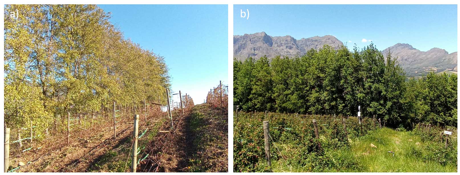
Figure 1 Images from the field site taken in (a) winter and (b) late spring. © Anton Kunneke.

The geological setting is formed by granites, quartz-porphyry and syenite (Schifano et al., 1970) from which a cambic mollic Umbrisol developed (IUSS Working Group WRB, 2015). The field site is situated roughly 400 m above mean sea level, and the slope is inclined by approximately 15 %.

The site is part of a working fruit farm, and the studied field is under current cultivation with blackberry (Rubus fruticosus L. Var. “Waldo”), divided by linear windbreaks consisting of pure Italian alder (Alnus cordata (Loisel.) Duby). The blackberry canes are aligned in parallel rows with a between-row distance of 2.5 m. At the time of study, the blackberry canes at the site were 5 to 6 years old; these usually start developing shoots in late spring (October), and the berries are harvested from mid-January to mid-March. The plants are irrigated with a dripper system during summer (November–January), roughly three times per week for 1.5 h at a rate of 2.3 L h⁻¹. Slow-release fertiliser is applied once a year just before spring.

Our measurement campaign focused on two berry plots and the adjacent alder windbreaks. The windbreak between the berry plots was studied in more detail. It consists of one single row (45 m long) of alder trees, approximately 15 to 20 years old, and is linearly oriented from east-northeast to west-northwest. Individual trees are planted at a regular spacing of approximately 70 cm. The trees developed very particular crown shapes, perpendicular to the windbreak axis, with the exception of edge trees which have a rounded crown. Impressions of the site and the differences in the seasonal appearance are shown in Fig. 1.

3 Measurement setup

A joint interdisciplinary field campaign took place in September 2019. This activity included the extraction of soil samples for texture determination and nutrient and soil organic carbon analysis, along transects across the two berry plots and adjacent windbreak. Additional sampling with larger cylinders was done to determine soil hydraulic characteristics. To characterise and classify the soil, a profile was dug, described and sampled. Scanning the windbreak between the two berry plots with terrestrial lidar was coupled with manual measurement of the windbreak trees. Additionally, various sensors were installed to continuously monitor meteorological and soil hydrological variables in the subsequent months. A map of the study site is shown in Fig. 2. All measurements are described in more detail in the following sections.

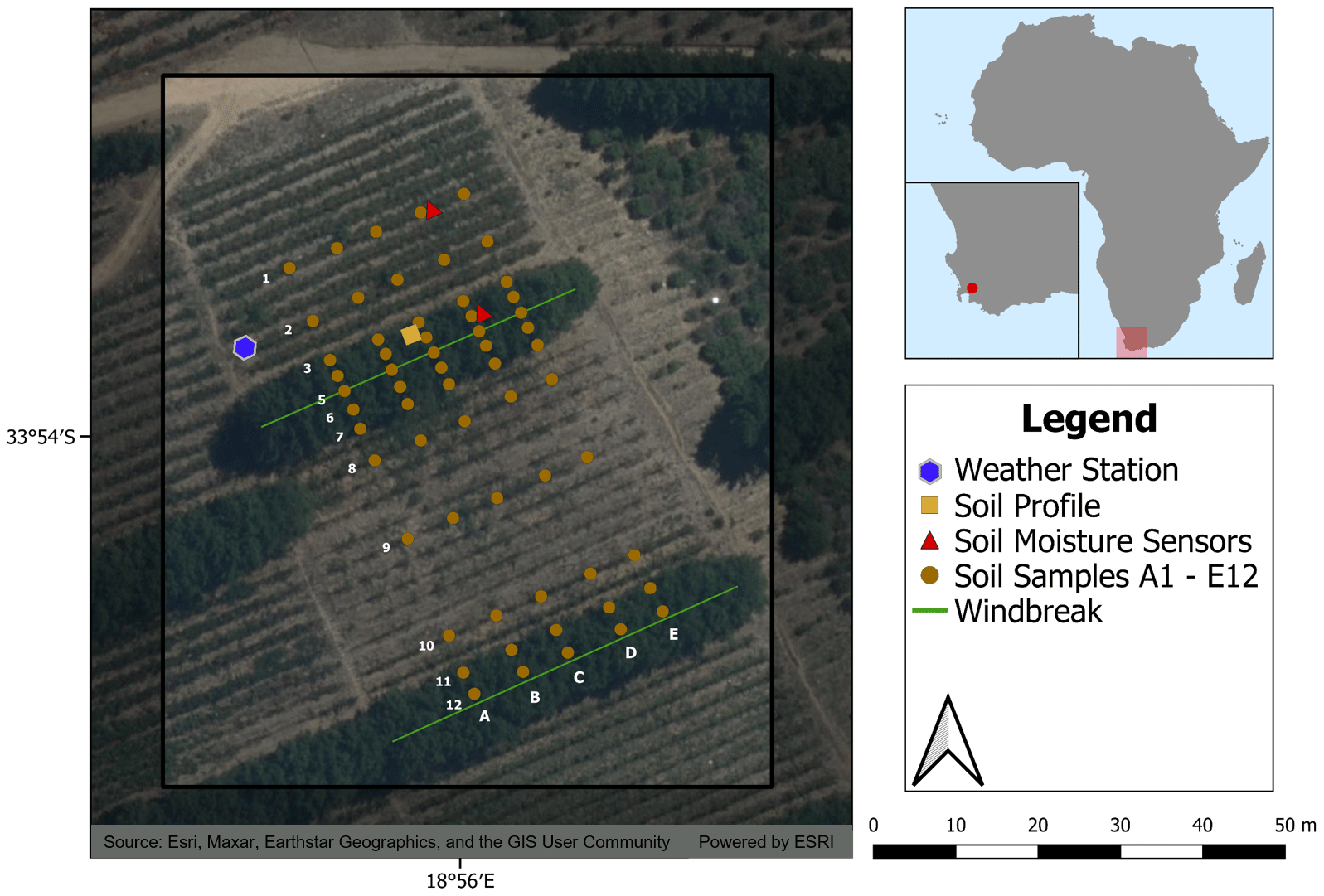
Figure 2 Map of the study site showing the location of the measurements of the field campaign (from the data description in Hassler et al., 2024).

3.1 Meteorological variables

3.1.1 Measurements

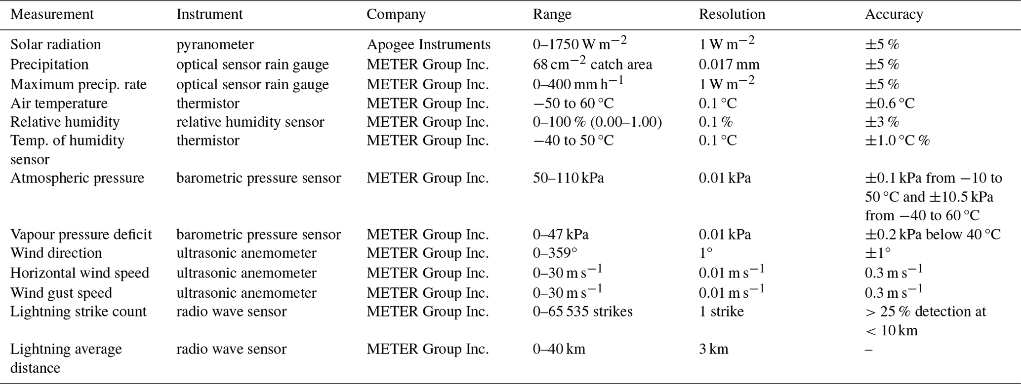
Meteorological data were recorded with an ATMOS 41 weather station in combination with a ZL6 cloud data logger (both METER Group Inc., Pullman, USA). Figure 2 shows the position of the weather station in the study site. A list of the measured variables and their sensors (along with range, resolution and accuracy) is compiled in Table 1. A rough overview of the resulting time series is attached in Appendix A1.

Table 1 Sensor characteristics for the meteorological measurements. All sensors are part of the setup of the ATMOS 41 weather station (METER Group Inc., Pullman, USA).

3.1.2 Data processing and quality control

Data were recorded in 10 min intervals from 19 September 2019 until 18 June 2021. The time zone utilised is coordinated universal time (UTC). Sensors were installed 2 m above ground level. During high-precipitation events, the ultrasonic anemometer recorded unusually high values. This error was on occasion also experienced in the mornings, probably due to dew accumulation. All events in question were referenced with the climate station at Stellenbosch airport, and wind speed and gust speed were manually filtered as “NA” whenever values seemed unreasonable. The procedure was straightforward, as most of the unusual values exceeded the maximum possible 30 m s⁻¹ of the sensor on low-wind days. It should be taken into account that wind speeds are significantly reduced by the windbreak when the wind is blowing in a southerly direction, which leads to considerable differences in wind speeds when wind direction changes frequently in short periods of time. The accuracy of the humidity sensor is generally slightly lower in a high-humidity environment as it is a temperature-dependent variable that shows large fluctuations with small changes in temperature, i.e. the higher the number of vapour particles detected. The ATMOS 41 weather station measures precipitation as individual droplets to also reflect dew formation with high accuracy and queries appropriate accumulations once every minute. Precipitation is then given as the cumulative amount per chosen measurement interval. The maximum precipitation rate is referenced to hourly values by multiplying maximum rainfall accumulation for 1 min periods by 60 min h⁻¹.

3.2 Hydrological measurements

We studied the influence of the windbreak on water fluxes in the berry plot by monitoring soil moisture and matric potential. Additionally, we took soil samples to characterise soil hydraulic characteristics under laboratory conditions.

3.2.1 Soil moisture and matric potential

Soil moisture was monitored continuously with time-domain reflectometry (TDR) probes (PICO-PROFILE T3PN, IMKO GmbH, Ettlingen, Germany) at two locations at four different depths (Fig. 3) from 21 September 2019 to 14 March 2020. The probes were installed in acrylic glass access tubes (diameter of 4.4 cm). One tube was installed within the rhizosphere of the windbreak, in the first berry row (referred to as “windbreak + berries” in the following). The other tube was installed close to the eighth berry row from the windbreak (“berries”; reference location) to minimise its influence. In each tube, we installed four TDR probe segments, stacked directly on top of each other, to allow for a continuous soil moisture signal along the profile. Each probe segment had a length of 18 cm and a penetration depth of the microwave impulse of 5.5 cm, so the soil moisture signal was integrated over a volume of approximately 1 dm³. The total profile depth we could measure was subsequently about 0.8 m, which should cover a prominent influence zone of the tree roots in the windbreak + berries tube (Kutschera and Lichtenegger, 2002), allowing for comparisons with the reference location.

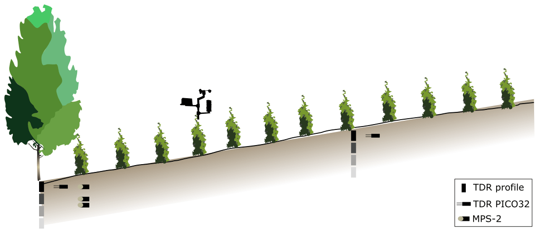
Figure 3 Slope cross-sectional sketch with the monitoring setup to study the water fluxes. The soil samples for measuring soil hydraulic characteristics in the laboratory are not included in the sketch; the profile samples were taken adjacent to the monitoring setup close to the windbreak, and the 12 extra samples were taken directly next to the windbreak and in the reference berry row.

Additionally, we installed two TDR probes (Trime PICO-32, IMKO GmbH, Ettlingen, Germany) with a measurement volume of approximately 0.25 dm³, one next to each tube, at 10 cm depth to capture the likely more dynamic soil moisture changes close to the surface (Fig. 3). Adjacent to the windbreak + berries tube location, we also installed three dielectric water potential sensors (MPS-2, Decagon Devices Inc., Pullman, WA, USA) in a profile at depths of 0.1, 0.3 and 0.4 m (Fig. 3) to gain more insight into the water tension in the soil at different depths under the influence of the tree roots. The monitoring measurements were recorded with a Truebner TrueLog100 (Truebner GmbH, Neustadt, Germany) data logger in 15 min intervals. An overview of the sensors and their range, resolution, and accuracies can be found in Table 2; a figure of the resulting measurement time series is included as Fig. 4.

Table 2 Sensor characteristics for the hydrological measurements as given by the manufacturer (VWC: volumetric water content).

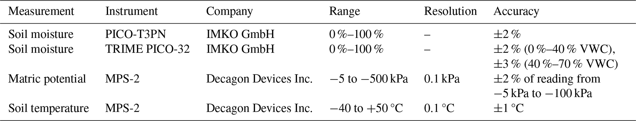
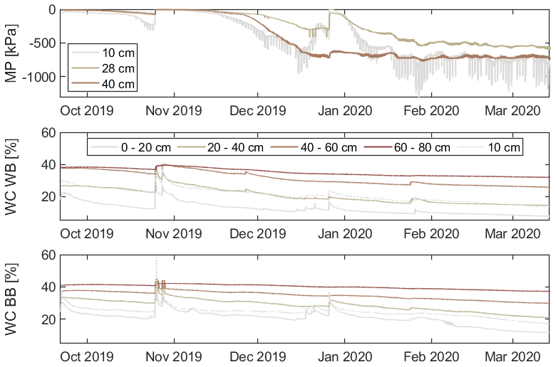
Figure 4 Time series of soil moisture and matric potential over the course of the monitoring period. WC: water content, MP: matric potential, WB: the windbreak + berries measuring location, BB: reference location berries.

3.2.2 Soil hydraulic characteristics

Undisturbed 250 mL cylindrical soil samples were taken to measure soil hydraulic characteristics in the laboratory. Three samples were extracted from a soil profile adjacent to the soil hydrological measurements at the windbreak (Fig. 3). The samples were taken at the surface and at depths of 0.3 and 0.5 m right after installation of the sensors on 16 September 2019. In a sampling campaign in March 2022, 12 additional samples were taken to enable a more comprehensive assessment. They were located at three points (east, middle and west) directly adjacent to the windbreak, as well as at three points within the reference berry row (eighth row from the windbreak), always at 5 and 25 cm depths.

Soil texture analysis was conducted through wet sieving (without soil skeleton of particle diameter d_p>2 mm) into the classes of coarse sand (2 mm $>d_{\mathrm{p}}>\mathrm{630}$ µm), medium sand (630 µm $>d_{\mathrm{p}}>\mathrm{200}$ µm) and fine sand (200 µm $>d_{\mathrm{p}}>\mathrm{63}$ µm). Before, organic compounds were destroyed through the application of hydrogen peroxide. Smaller fractions were separated with the sedimentation method according to DIN ISO 11277 (ISO, 2002) into coarse silt (63 µm $>d_{\mathrm{p}}>\mathrm{20}$ µm), medium silt (20 µm $>d_{\mathrm{p}}>\mathrm{6.3}$ µm), fine silt (6.3 µm $>d_{\mathrm{p}}>\mathrm{2}$ µm) and clay (d_p<2 µm).

Soil hydraulic conductivity of the undisturbed samples was measured with the KSAT apparatus (UMS GmbH, Munich, Germany). The measurement is following the Darcy approach, applying water flux through a saturated porous medium. The apparatus records the falling head of the water supply though a highly sensitive pressure transducer which is used to calculate the flux.

Soil water retention characteristics were measured on the same samples in the HYPROP apparatus (UMS GmbH, Munich, Germany) and afterwards in the WP4C (PotentiaMeter, Decagon Devices Inc., Pullman, WA, USA). The HYPROP registers matric head at two depths and the total weight of the sample while it is drying out by free evaporation. The maximum water tension that can be measured with this method is about −800 hPa and is limited by the air entry point of the tensiometer. After measurement in the HYPROP, a small subsample of about 10 g was transferred to the WP4C where soil water potential is measured using a chilled-mirror approach.

The measurements of water tension and water content from the HYPROP and WP4C were used to derive water retention curves (Fig. 5), parameterised with the van Genuchten equation (van Genuchten, 1980):

$$\begin{array}{}\text{(1)}& \mathrm{\Theta }\left(\mathit{\psi }\right)={\mathrm{\Theta }}_{\mathrm{r}}+{\displaystyle \frac{{\mathrm{\Theta }}_{\mathrm{s}}-{\mathrm{\Theta }}_r}{[\mathrm{1}+(\mathit{\alpha }\left|\mathit{\psi }\right|{)}^n{]}^{\mathrm{1}-\mathrm{1}/n}}},\end{array}$$

with the water retention curve Θ(ψ) in m³ m⁻³, the residual water content Θ_r in m³ m⁻³, the saturated water content Θ_s in m³ m⁻³, the scaling parameter inverse to the air entry suction α, the matric potential ψ and the dimensionless shape parameter n.

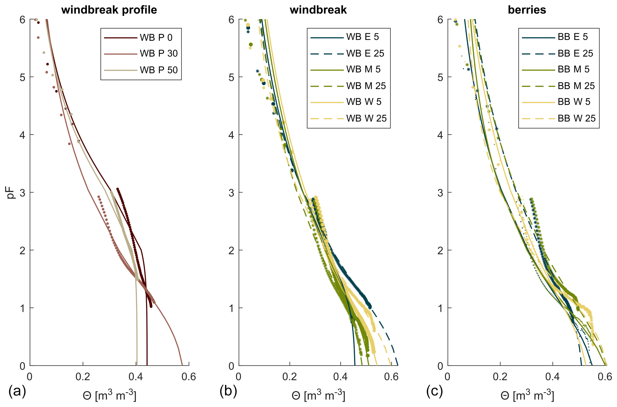
Figure 5 Soil water retention curves of the three profile samples at the windbreak (a, at 0, 0.3 and 0.5 m depth), six samples at three locations at the windbreak (b, at 0.05 and 0.25 m depths) and six samples at three locations in the berries (c, at 0.05 and 0.25 m depths). The dots and stars represent the water tension (pF, the log of the absolute value of the pressure in hPa) and water content measurements, and the lines show the fitted water retention curves after van Genuchten (1980). In panels (b) and (c), dots belong to the 0.05 m depths and stars to the 0.25 m depth.

3.2.3 Data processing and quality control

The in situ monitoring sensors recorded observations in 15 min intervals. The data were checked for inconsistencies, obvious erroneous values, and spikes or missing values. These could occur due to power outages or maintenance interruptions. The respective values were removed from the time series. The timestamp which was originally in local time was converted to the UTC time format for all time series.

An accuracy of 2 % can be reached with the IMKO sensors (T3PN and PICO-32) if the tubes/sensors are installed correctly with close contact to the soil. No site-specific calibration was done prior to or after installation, which can lead to errors in the absolute readings. Further, we did not correct for soil density deviations but used the standard soil calibration (1.40675 g cm⁻³).

The MPS-2 matric potential sensors frequently reached values of less than −500 kPa, which should not be used for quantitative analyses because of potentially large errors in the magnitude of the water potential.

It is plausible that some degree of error could have been introduced during installation of the sensors. However, drilling the vertical holes for the acrylic tubes was done with great care so that the tubes had good contact with the soil. Additionally, any space between the soil and the tube could be assumed to settle with time and with rain, so the measurement signal should be robust. Due to heterogeneities in the soil, the additional Trime PICO TDR sensors and the matric potential sensors may not have been installed within completely uniform soil conditions as a result of air pockets or rocks. This problem is difficult to avoid completely; however, during installation we did not observe any gross heterogeneities that would indicate concern.

When examining water fluxes and calculating water balances, the factor of irrigation should be kept in mind, as the additional water input cannot be exactly quantified.

3.3 Soil characteristics

Soil sampling took place during the joint field campaign in September 2019. We collected samples from a soil profile for soil classification and along transects to study the spatial differences in topsoil nutrient contents and texture (see Fig. 2).

3.3.1 Soil profile

In a freshly dug soil profile to a depth of 0.75 m, we defined soil horizons after visual inspection of colour changes and manual texture assessment (Fig. 6). The horizons were Ah1 (0–20 cm), Ah2 (20–40 cm), Bw1 (40–55 cm), Bw2 (55–75 cm) and C (>75 cm). From each horizon, we took one composite sample mixed from multiple individual ones, spread across the width of the soil pit and the depth of the respective horizon, using a hand shovel. We used these samples for texture analysis and determination of total carbon and nitrogen, as well as the potential cation exchange capacity (CECpot) and contents of exchangeable cations. These were carried out under laboratory conditions in Germany. A soil profile description and soil classification was subsequently carried out according to the World Reference Base for Soil Resources (IUSS Working Group WRB, 2015).

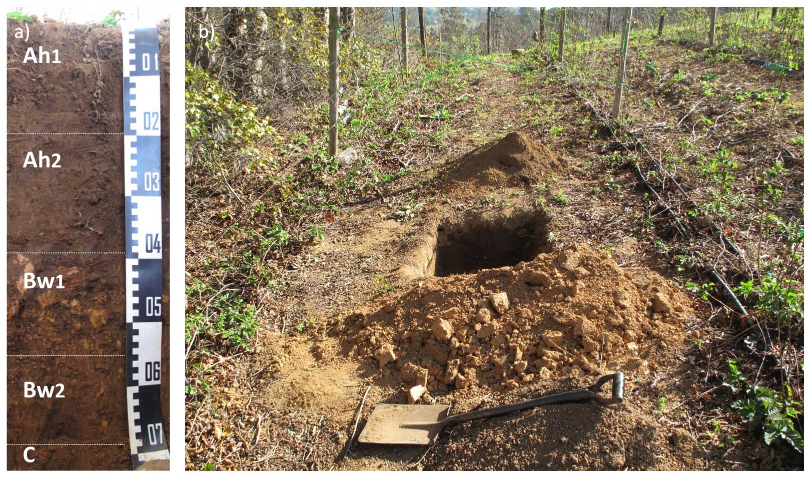
Figure 6 Soil profile: Dystric Cambisol (loamic, colluvic, humic) according to the IUSS Working Group WRB (2015). (a) Profile with the delineated horizons; (b) profile pit between the berry rows.

3.3.2 Transects

We further collected 60 soil samples along five parallel transects perpendicular to the slope, crossing the blackberry and alder rows (Fig. 2). Each transect held 12 sampling points in the alder and berry rows. To gain a better understanding of the spatial influence of the windbreak on topsoil characteristics, the distances between the samples close to the windbreaks were smaller (in every berry row), increasing towards the middle of the berry plots (serving as reference with no windbreak influence). The samples were taken in the topsoil (0–10 cm) with an ordinary hand shovel within the blackberry rows, between individual plants, avoiding the direct root environment. One sample of about 300 g was taken per sampling point. The samples were homogenised, air-dried and sieved (<2 mm), and two subsamples of each sample were transferred to Germany for laboratory analyses. Carbon and nitrogen contents were estimated at the Soil Ecology laboratory at the Chair of Soil Ecology at the University of Freiburg, Germany, and soil texture was estimated at the laboratory of the research area Landscape Functioning at the Leibniz Centre for Agricultural Landscape Research (ZALF) in Müncheberg, Germany.

3.3.3 Analytical procedures

The analyses carried out on the samples differed between the samples, depending on their research purpose. The profile samples were needed for soil classification, while the transect samples were taken in order to study the spatial variability in soil characteristics.

We determined residual water content of all soil samples by drying an aliquot at 105 °C and comparing wet and dry weights of the sample as most analysis methods are related to dry mass of soil. The pH value of the samples was measured in a 1:2 soil–water slurry with ultrapure water and with a glass electrode (Metrohm 751 GDP Titrino meter, Herisau, Switzerland).

To determine total carbon and nitrogen concentrations, subsamples of soil material were milled (Siebtechnik TEMA, Mülheim an der Ruhr, Germany), dried at 105 °C, combusted at 1150 °C and measured with an elemental analyser (Vario EL cube, Elementar, Langenselbold, Germany). This was done for both the profile and the transect samples. Exchangeable base cations calcium (Ca), magnesium (Mg), potassium (K) and sodium (Na) as well as potential cation exchange capacity (CECpot) were extracted with 1 M ammonium acetate at pH 7 according to the ammonium acetate method (van Reeuwijk, 2002) of the soil profile samples only. Cation concentrations in extracts were measured with an inductively coupled plasma optical emission (ICP-OE) spectrometer (Spectro Ciros CCD ICP side-on plasma optical emission spectrometer, Kleve, Germany). The percentage of base saturation was calculated from the results of exchangeable cations and CECpot.

The soil texture for the profile samples was determined after previous destruction of organic matter with combined methods of sieving and sedimentation according to DIN ISO 11277 (ISO, 2002). This was carried out at the Soil Ecology laboratory, University of Freiburg, Germany.

The soil texture for the transect samples was analysed without destroying organic material in order to obtain the effective particle size distribution along the transects throughout the cultivation system, and only the laser diffraction method was used. After using Na₄P₂O₇ as a dispersing agent, the sand fraction was obtained by sieving the soil solution through a 63 µm mesh. These sieved particles were dried at 105 °C, and the sand fraction was calculated as the ratio of sand to total dried soil sample mass. A subsample of the suspension was transferred to the wet dispersion unit of the Mastersizer 3000 and stirred (3500 rpm and 100 % sonication power) until the laser obscuration level reached 10 %. Clay and silt contents were calculated according to the method for laser diffraction particle size analysis presented in Faé et al. (2019). This was carried out in the laboratory at ZALF, Müncheberg, Germany.

3.3.4 Data processing and quality control

Soil sampling was carried out according to the FAO Guidelines for soil description (Jahn et al., 2006). The analysis of physical and chemical soil parameters followed standard methods described in the Procedures for Soil Analysis (van Reeuwijk, 2002) and according to DIN ISO 11277 (ISO, 2002). The quality of the nutrient analyses was continuously checked and calibrated using external standards. We used Certipur ICP multi-element standard solution IV (Merck KGaA, Darmstadt, Germany). Additionally, we measured an internal soil standard with known nutrient contents together with the samples. The analyses of CECpot and exchangeable base cations were performed in triplicate.

3.4 Dendrological measurements

The research site was scanned in September 2019 with the RIEGL VZ 2000i terrestrial lidar (RIEGL Laser Measurement Systems GmbH, Horn, Austria), set with a pulse repetition rate of 600 kHz, and reported with a laser beam divergence of 0.27 mrad (an increase of 27 mm of beam diameter per 100 m distance). A multiple-scans approach was used under negligible wind conditions. We derived 3D point clouds from the scans and processed these to obtain structural tree data, foliage data and windbreak characteristics. We also measured diameter at breast height (DBH) and between-tree spacing manually, in order to cross-reference the point cloud data.

3.4.1 3D data processing

Co-registration was carried out using the software RiSCAN PRO 2.11.3 (RIEGL Laser Measurement Systems GmbH, Horn, Austria) and following the software-guided steps for coarse registration of point clouds in an outdoor non-urban scenario; we used multi-station adjustment 2 for the fine registration in the same software. In total, 42 scanning positions focusing on the windbreak structure were selected to represent the study area. These had a varied scanning step of 5 to 30 m between scanning points. The isolated points and single-scan points further than 60 m were removed. The exported project point cloud was made homogeneous by applying cubic downsampling (25 mm voxel side) and saved as a LAZ file (1.4 format), including many attributes of the laser data. A video animation is included with the data in the repository for an overview of the research area.

The windbreak point cloud included 32 scanning positions covering the target windbreak trees. From the linear windbreak structure, 14 scanning positions were within 10 m distance from the target windbreak, and they were distant from each other by 5 to 10 m. The remaining 18 positions were located between 15 and 25 m away from the windbreak base. Trees were partially under leaf-off conditions as scanning took place in early spring, but some trees had retained leaves from the previous season. The presence of obstacles within the site, i.e. the support structures for the blackberry crop, made movement within the field difficult and formed obstructing structures within the laser's field of view, leading to occlusion of the deep crown and lower parts of the stem.

3.4.2 Tree data

The studied windbreak section was extracted from the co-registered project point cloud and filtered by pulse deviation (equal or lower than 10; Pfennigbauer and Ullrich, 2010). Isolated points were removed, and the windbreak point cloud was exported as a separate file. From within the windbreak point cloud, starting from the east-northeast edge in a west-southwest direction, 18 single-tree point clouds were manually segmented, thus isolating them from the point cloud as a whole, and sequentially labelled t01 to t18. These were further processed by filtering out foliage points (utilising reflectance and RGB values), while duplicated points, noisy points and outlier points were removed using CloudCompare v2.10.2 (CloudCompare, 2019). Lastly, the individual tree point clouds were separated into three occlusion category classes regarding occlusion of the woody components, namely low, mid and high occlusion levels.

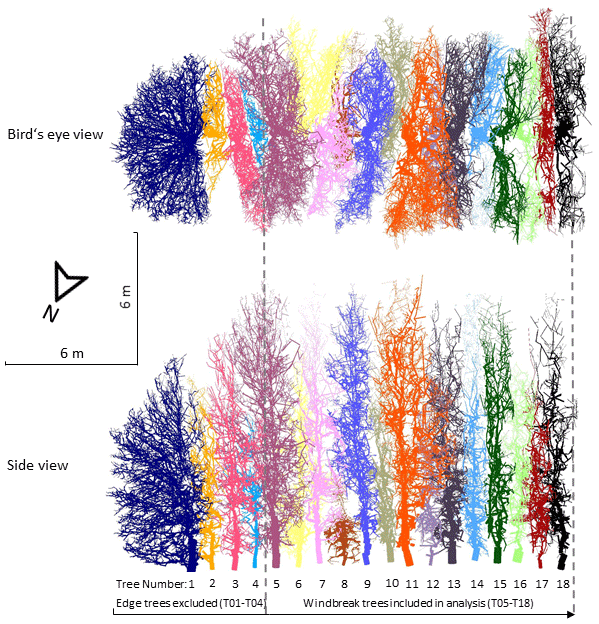
Figure 7 A bird's eye view and a side view of cylinder models of the sample windbreak. Colour denotes individual trees. Trees 1–4 (t01 to t04) were excluded from the analysis due to the windbreak edge influencing the growth form.

The single-tree point clouds were used for producing cylinder models in the form of quantitative structure models (QSMs) with the MATLAB implementation of TreeQSM v2.3 (Raumonen et al., 2013). Following the framework of Calders et al. (2015), QSMs were optimised by testing 72 combinations of inputs over 25 runs, and best models were selected using the “mean point-cylinder distance” as metric. Tested parameters were the following (in metres): PatchDiam1 (0.30, 0.25, 0.15, 0.10), PatchDiam2Min (0.015, 0.02, 0.03), PatchDiam2Max (0.05, 0.07, 0.09) and lcyl (4, 6, non-metric). The optimised input parameters and the precision of the QSM estimates are provided within occlusion category classes. Other QSM parameters employed were FilRad (3.5) and nmin1 (4). The model output is shown in Fig. 7; there, side and bird's eye views of the windbreak are shown, and individual trees are shown in different colours; note that trees t01 to t04 were not considered for analysis due to a differing growth form attributed to the edge effect. Volumetric tree parameters were converted to biomass using a wood density of 420 kg m⁻³, considering an average value for Alnus sp. (after Harja et al., 2023). The coarse root biomass (roots with >2 mm cross-sectional diameter) was estimated as 28.54 % of the total aboveground woody biomass (Frouz et al., 2015), defined as belowground biomass and also converted to volumetric terms.

3.4.3 Foliage data

Foliage data were retrieved by applying the leaf creation algorithm (LCA) after Bohn Reckziegel et al. (2021) to the QSMs of trees t05 to t18. According to leaf sizes as described for Alnus sp. by the European Atlas of Forest Tree Species (San-Miguel-Ayanz et al., 2016), the LCA was modified to restrict the use of the leaf classes to small, medium and large categories, with corrected proportions. The parameter leaf spacing was defined to values of 2.0, 2.5, 3.0 cm, and total leaf area was estimated on a tree basis. Leaf dry mass was estimated using the specific leaf mass of 13.3 ± 0.3 m² kg⁻¹ for (Alnus glutinosa (L.) Gaertn.) as given by Johansson (1999).

3.4.4 Windbreak properties

Windbreak properties were assessed upon the acquired 3D data (terrestrial lidar), the assessment of tree structure with QSMs and the generated foliage data. A number of windbreak properties from the windbreak point cloud were derived from manipulation using CloudCompare v2.10.2 (CloudCompare, 2019), namely length, width, tree number and tree spacing, for the entire windbreak. Average values for the QSM-derived attributes of measured trees were also computed for trees t05 to t18. Tree volume and biomass, as well as total leaf area and leaf mass, were estimated per metre of windbreak. Plant coverage was derived as the ratio of the alpha-convex hull (ahull function from the “alphahull” package by Pateiro-Lopez and Rodriguez-Casal, 2019) of leaf points and the minimum binding box (getMinBBox function from the “shotGroups” package by Wollschlaeger, 2022) in R v4.0.4 (R Core Team, 2021). Leaf area index (LAI) was derived as the total leaf area by the canopy projection area, defined as an alpha-convex hull.

3.4.5 Data processing and quality control

The processing of the 3D data followed a standard protocol within terrestrial lidar analyses (e.g. Raumonen et al., 2013). QSM precision was assessed utilising occlusion categories based on input parameters within the QSM modelling process as described above. Due to the highly dense vegetation and field obstacles, a complete coverage of the windbreak was impeded. Optimisation was applied to control the precision of the tree reconstruction. The validation of tree measurements would require destructive sampling of trees, which was not permitted; nevertheless, past studies have shown high correlation between traditional measurement techniques and lidar-derived data (e.g. Kuekenbrink et al., 2021; Calders et al., 2015; Raumonen et al., 2015). The non-destructive foliage data simulation used the LCA (Bohn Reckziegel et al., 2021) and was facilitated by a robust reconstruction of the trees with optimised QSMs. Nevertheless, the LCA results may be subject to errors, i.e. at the top of the QSMs due to lower point density, and due to varying foliage capacity of a tree (ecophysiological state). The description of tree windbreaks with parameters derived from 3D data assist the characterisation of these vegetative structures, enabling the estimation of many hard-to-measure tree attributes.

4 Applications

The multidisciplinary focus of the complete dataset package allows for various analysis avenues. The main research goal we wanted to target by collecting these data was to assess the influence of the windbreak in this AFS on water fluxes, nutrient distribution and microclimate in the crop. The corresponding scientific study is Hoffmeister et al. (2024). By combining the different measurements, the effects of the windbreak were clearly visible, as well as the effect of the irrigation in the system. The latter influenced the water balance by reducing water limitation, securing sufficient water for plant growth. The windbreak also needed water to grow; however, it also lowered the irrigation demand for the blackberry crop by reducing soil evaporation and influencing water redistribution. Nutrient accumulation near the windbreak and the occurrence of water erosion were indicated by soil physiological properties and nutrient distribution. Additionally, the windbreak increased the carbon sequestration potential compared to monoculture farming.

The detailed information on site conditions as well as the high-resolution time series of meteorological parameters, soil moisture and matric potential enables hydrological modelling studies on the slope scale. Once parameterised, scenarios can be run to elucidate the shifts between water limitation and energy limitation in the AFS and to inform about possible management strategies to utilise the windbreak influence.

The availability of the point cloud data acquired with terrestrial lidar facilitates the three-dimensional examination of the studied windbreak in high detail. This allows for scrutiny of sections of the windbreak row, individual trees or tree parts thereof, and this can be carried out within the context of the study of AFSs, Alnus sp. or for those interested in vegetative windbreak structures. Moreover, the dataset provides a unique view on a frequent, though not often understood, and alternative spatial arrangement of trees with specific tree growth conditions, which differ from forest formations, stands and scattered trees. The point cloud dataset offers the possibility to use it as an independent training dataset limited in size and spatial complexity.

The variety of measurements across different ecosystem compartments also supports studying the interactions between these compartments, which is rarely possible in otherwise mostly discipline-specific campaigns. Additionally, the measurements serve as an example of a (for the region typical) AFS including windbreak and crop and can be compared to other windbreaks and to other AFSs. This enables further insights into the varied interactions between the different components of these systems to help elucidate benefits and limitations of introducing AFSs as a sustainable land use option in a changing climate.

Limitations of the dataset include its limited geographical scope, as we only measured at one AFS on one slope at the one location. Further specifics of the site should also be kept in mind when using the data. For example, the irrigation scheme, of which we only have estimates and no accurate values, will affect any attempted water balance calculations. Additionally, the meteorological variables are affected by the windbreak influence on the wind field.

5 Data availability

The described datasets are freely available and accompanied by a technical description of the individual tables from the online repository GFZ Data Services and are published under https://doi.org/10.5880/fidgeo.2023.028 (Hassler et al., 2024). The data files in the repository are named according to their respective research discipline: meteorology (“_Meteo_”), hydrology (“_Hydro_”), soil science (“_ Soil_”) and dendrology (“_Dendro_”). They include time series for the meteorological variables, soil moisture and matric potential as well as data from the joint measurement campaign, namely nutrient, cation, and texture data for the soil samples; soil hydraulic characteristics from the cylinder samples; and the derived tree and windbreak characteristics from the terrestrial laser scans.

6 Conclusions

Interdisciplinary and multivariate field campaigns are notoriously challenging; expectations and requirements for the field sites vary between the different groups, and there are never enough measurements that can be taken to really cover all aspects of the ecosystem satisfactorily. Our dataset was intended as an example to enable studying various influences of the tree components in this AFS and also to be compared to similar measurements in other AFSs. Despite some limitations, it provides a glimpse into the relevant processes and opens up further avenues to assess and promote AFSs as a sustainable land use type in a changing world.

Appendix A: Overview of meteorological time series

We provide an overview of the time series of meteorological measurements (Fig. A1), primarily to give a first idea of what kind of data, dynamics and ranges are included in the data files. Some of the, most likely, less important time series (maximum precipitation rate, temperature of the humidity sensor, wind direction, gust speed, and lightning count and distance) are omitted from the figure to make it clearer.

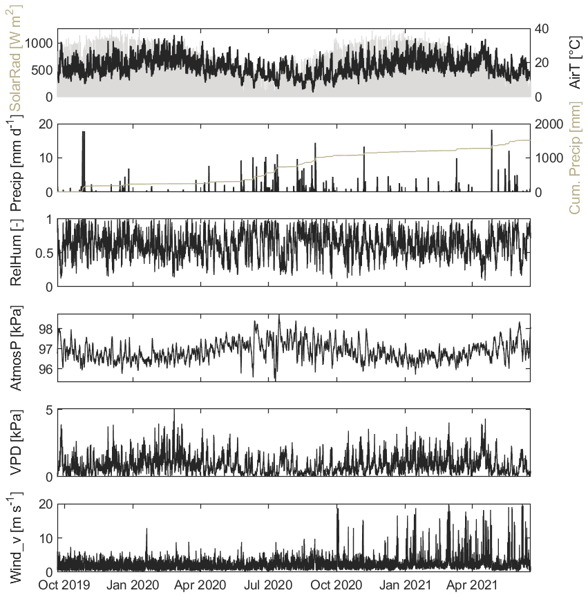
Figure A1 Time series of meteorological variables over the course of the monitoring period. Shown are solar radiation (SolarRad), air temperature (AirT), precipitation (Precip), cumulative precipitation (Cum. Precip), relative humidity (RelHum), atmospheric pressure (AtmosP), vapour pressure deficit (VPD) and wind velocity (Wind_v).