A global catalogue of CO₂ emissions and co-emitted species from power plants, including high-resolution vertical and temporal profiles

We present a high-resolution global emission catalogue of CO₂ and co-emitted species (NO_x, SO₂, CO, CH₄) from thermal power plants for the year 2018. The construction of the database follows a bottom-up approach, which combines plant-specific information with national energy consumption statistics and fuel-dependent emission factors for CO₂ and emission ratios for co-emitted species (e.g. the amount of NO_x emitted relative to CO₂: ${\mathrm{NO}}_x/{\mathrm{CO}}_{\mathrm{2}}$). The resulting catalogue contains annual emission information for more than 16 000 individual facilities at their exact geographical locations. Each facility is linked to a country- and fuel-dependent temporal profile (i.e. monthly, day of the week and hourly) and a plant-level vertical profile, which were derived from national electricity generation statistics and plume rise calculations that combine stack parameters with meteorological information. The combination of the aforementioned information allows us to derive high-resolution spatial and temporal emissions for modelling purposes. Estimated annual emissions were compared against independent plant- and country-level inventories, including Carbon Monitoring for Action (CARMA), the Global Infrastructure emission Database (GID) and the Emissions Database for Global Atmospheric Research (EDGAR), as well as officially reported emission data. Overall good agreement is observed between datasets when comparing the CO₂ emissions. The main discrepancies are related to the non-inclusion of auto-producer or heat-only facilities in certain countries due to a lack of data. Larger inconsistencies are obtained when comparing emissions from co-emitted species due to uncertainties in the fuel-, country- and region-dependent emission ratios and gap-filling procedures. The temporal distribution of emissions obtained in this work was compared against traditional sector-dependent profiles that are widely used in modelling efforts. This highlighted important differences and the need to consider country dependencies when temporally distributing emissions. The resulting catalogue (https://doi.org/10.24380/0a9o-v7xe, Guevara et al., 2023) is developed in the framework of the Prototype System for a Copernicus CO₂ service (CoCO2) European Union (EU)-funded project to support the development of the Copernicus CO₂ Monitoring and Verification Support capacity (CO2MVS).

1 Introduction

Over 40 % of fossil-fuel-related carbon dioxide (CO₂) emissions are caused by power plants that burn fuels to produce electricity and/or heat (Crippa et al., 2022). A correct representation of the spatial and temporal distributions of these point sources is important for verification of global CO₂ emissions through current and future satellite emission monitoring and inverse modelling efforts, like the envisioned European CO₂ Monitoring and Verification Support capacity (CO2MVS; Balsamo et al., 2021). The CO2MVS, which is planned to be fully operational by 2026, combines information from various observational datasets (i.e. satellite data from existing or new Copernicus Sentinel satellites and in situ data from various surface networks) and prior knowledge (i.e. mainly bottom-up emission estimates from inventories and reporting) with detailed Earth system modelling and data assimilation capabilities. The final goal of the CO2MVS capacity is to provide observation-based estimates of CO₂ emissions at multiple scales (i.e. from global to local industrial and urban hotspots) with a similar level of robustness that has proven critically important in other Copernicus Atmosphere Monitoring Service (CAMS) applications, such as air quality predictions (https://atmosphere.copernicus.eu/air-quality, last access: January 2024). Reducing the uncertainty in the inversion system, having higher accuracy in the final predicted emission estimates, and having high spatial and temporal resolution data for CO₂ emissions and co-emitted species (e.g. NO_x, CO), which are also used to derive observation-based CO₂ emissions as they can be detected more easily in satellite images (e.g. Kuhlmann et al., 2021), are key elements.

Spatial representation of large point sources in global state-of-the-art and/or widely used gridded emission inventories such as the Emissions Database for Global Atmospheric Research (EDGAR, Janssens-Maenhout et al., 2019) and the Open-Data Inventory for Anthropogenic Carbon dioxide (ODIAC, Oda et al., 2018) is primarily based on the Carbon Monitoring for Action (CARMA; Wheeler and Ummel, 2008), which was built using plant-level information from 2009 and is no longer maintained. Moreover, these inventories do not report emissions from facilities at their exact geographical locations but in the centroid of the respective inventory grid cells, which typically have a resolution of 0.1×0.1^∘. Subsequently, deviations from their exact locations can be up to a few kilometres. While this fact does not entail limitations for modelling applications working at the same or lower spatial resolutions (e.g. Agustí-Panadera et al., 2022), it may become critical for local and very-high-resolution modelling applications (e.g. Brunner et al., 2023). The more recently developed Global Infrastructure emission Database (GID, Tong et al., 2018) overcomes this limitation by providing up-to-date information and high-resolution CO₂ emissions from global power plants at the facility level. However, the latitude and longitude coordinates of each facility are not publicly available. Instead, georeferenced data are distributed in gridded format at a 0.1×0.1^∘ resolution. Moreover, no information is provided on how to distribute the emissions from each plant temporally and vertically, two parameters that are also essential for modelling purposes (e.g. Brunner et al., 2019; Guevara et al., 2021).

Here we present a global catalogue of CO₂ emissions and co-emitted species (i.e. NO_x, SO_x, CO and CH₄) from power plants at a high spatial and temporal resolution for the year 2018. The dataset contains annual emission information for individual thermal power plants that burn coal, natural gas, oil, solid biomass and municipal or industrial solid waste (hereinafter referred to as waste) to produce electricity or combined heat and electricity at their exact geographical location. Moreover, each facility is linked to a country- and fuel-dependent temporal profile (i.e. monthly, day of the week and hourly) and a facility-level vertical distribution profile, which allow us to derive spatially and temporally resolved emissions for modelling efforts.

Section 2 of the paper describes the methodology and databases considered for the construction of the global point source database, while Sect. 3 presents the main results and compares them against existing emission inventories at the plant, grid and country levels. Section 4 provides a description of the data availability, Sect. 5 lists the main limitations of the dataset, and finally Sect. 6 presents the main conclusions and future perspectives.

2 Methodology

The approach to construct the global point source database is divided into five phases: (1) selection of facilities and definition of associated geographical locations (i.e. latitude and longitude coordinates), (2) fuel allocation per facility, (3) estimation of annual emissions of CO₂ and co-emitted species (i.e. NO_x, SO_x, CO and CH₄) per facility, (4) construction of the monthly, weekly (day of the week) and hourly (hour of the day) temporal profiles associated with each facility and (5) construction of the vertical distribution profiles associated with each facility.

The global point source database is a mosaic constructed using as a basis the European and global power plant databases described in Sect. 2.1. The temporal and vertical profiles associated with each plant are constructed following a common approach that uses as a basis information on measured electricity statistics and plume rise calculations, respectively (Sects. 2.4 and 2.5, respectively). The sources of information and the approaches used to develop each dataset are described in the following sub-sections.

2.1 Compilation of facilities and geographical locations

To compile information on each individual power plant, including its name and exact geographical location, several public and commercial datasets were combined (Table 1). For the European database, the data sources used are the European Pollutant and Transfer Register database (E-PRTR_v18; EEA, 2020), the Large Combustion Plants database (LCP_v5.2; EEA, 2019), the Platts World Electric Power Plant dataset (WEPP Europe, September 2015, Platts, 2015) and the integrated Industrial Reporting Database (IRD_v7; EEA, 2022). For the non-European database, the datasets considered included the Global Coal Plant Tracker (GCPTv2021_01; GEM, 2021a), the Global Gas Plant Tracker (GGPTv2021_02; GEM, 2021b), the Global Power Plant Database (GPPDv1.3.0; Global Energy Observatory et al., 2021), the IndustryAbout database (IndustryAbout, 2021), the Emissions and Generation Resource Integrated Database (eGRIDv2018; US EPA, 2020), the Chinese Ministry of Ecology and Environment's domestic waste incineration power plant database (MIEE, 2022), the Tai biomass power plant database (DEDE, 2020), the Geocomunes Mexican power plant database (Geocomunes, 2020), the Taiwanese waste-to-energy plant database (Taiwan EPA, 2014), the electrical Japan power station database (Electrical Japan, 2022), the Argentinian renewable power plant database (MINEM, 2022) and the UNFCCC Clean Development Mechanism database (UNFCCC CMD, 2022). For both the European and non-European databases, substantial effort was put into identifying missing and incorrect facility geographical locations. Coordinates were checked or searched manually using Google Maps or other websites and added to the dataset as follows.

• For Europe, the reported coordinates were consistently checked and corrected for the top 100 facilities (in terms of 2017 CO₂ emissions). Furthermore, all coordinates that did not fall within the correct country borders or that were inconsistent between the reported dataset versions were manually checked and corrected. In addition, many other coordinates (likely about 400) were checked during the process of linking up facilities between datasets, identifying fuel types and looking at the resulting emission maps. In total, all the checks resulted in 360 plants with corrected coordinates, including about 75 of the top 100 plants.

• For the non-European dataset, the review process was performed for selected countries that are among the top 30 countries in terms of installed power generation capacity and that are representative of coal (i.e. South Africa, Japan, Taiwan, Kazakhstan, Australia, Vietnam and Turkey), natural gas (i.e. Japan, Oman, Thailand, Bahrain, Algeria and Ukraine) and oil (i.e. Egypt, Iran, Iraq, Libya, Pakistan and Saudi Arabia) power plants. In both cases, some corrections improve the coordinates by only tens of metres or less, and in other cases the original coordinates were further off. Multi-unit power plants were in most of the cases located at the same coordinates, since the distance between the units is usually small (i.e. dozens of metres). However, in facilities where the distance between the units was significant (i.e. a few kilometres), the original coordinates were edited and assigned to individual units. Despite these efforts, there may still be some errors present in the dataset, especially in the case of small plants.

Table 1 The main characteristics of the power plant databases considered in this work.

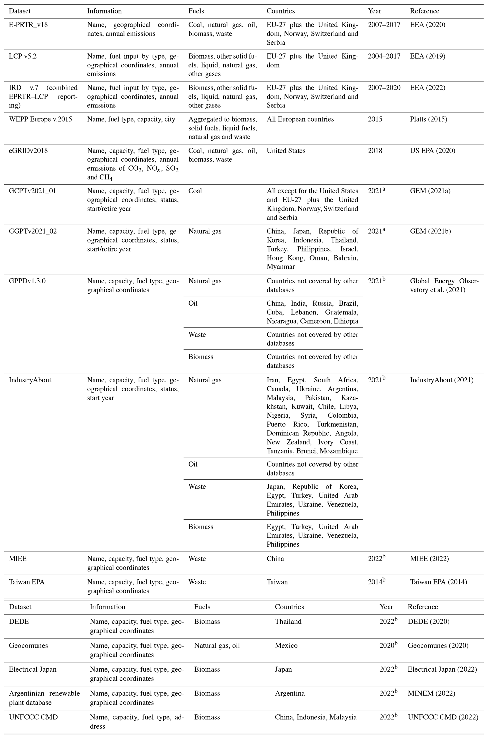
^a We only considered those facilities that were operating in 2018. ^b We assume that all the reported facilities were already or still operating in 2018.

2.2 Fuel allocation

Each of the emission values in the European power plant dataset is allocated to one of five fuel types (i.e. biomass, coal, oil, natural gas or waste). Three methods were used to allocate the fuel type.

1. Link to the LCP dataset: as LCP reporting includes the reporting of fuel input (but not for waste), this could be used to allocate emissions to different fuels when there was a link between E-PRTR and LCP facilities. Still, as only one emission value is reported, in the case of a multi-fuel plant (e.g. co-combustion of biomass in a coal-fired power plant), a proxy emission value for each fuel type was estimated using country- and fuel-specific emission factors from the Greenhouse Gas–Air Pollution Interactions and Synergies (GAINS) model at the International Institute for Applied Systems Analysis (IIASA) (Amann et al., 2011; Klimont et al., 2017). The ratio between the proxy emission values was then used to allocate the actual emission values to specific fuel types.

2. Link to the Platts WEPP dataset: if no LCP fuel data were available, for some plants the fuel type could be taken from a link to the Platts WEPP dataset. The Platts WEPP dataset contains a detailed fuel type for every electricity-producing unit and also lists the electric capacity for every unit. For those facilities that could not be successfully linked to an LCP plant, a link was made to electricity-producing units in the Platts WEPP database. The listed power and fuel type of the units were used together with country- and fuel-specific emission factors from the GAINS model to estimate a proxy emission value for each unit and to attribute the emissions to different fuel types.

3. There is manual search and allocation of fuel types for the 133 remaining plants.

For non-European power plants, we used the plant-level fuel information provided by the databases listed in Sect. 2.1, which only report the main fuel even in the cases of multi-fuel plants. Therefore, for each power plant, all the emissions are linked to one single fuel, as we did not have information to split emissions between fuels in multi-fuel plants as done for the European dataset. This limitation could have an impact on dual-fuel power plants that can use more than one fuel to operate (e.g. natural gas and diesel), as only emissions from its primary fuel will be allocated in them. To homogenise the results reported by the European and non-European datasets, we assigned to each European power plant the fuel with the largest contribution to the total CO₂ emissions.

2.3 Estimation of annual CO₂ emissions and co-emitted species

2.3.1 Europe

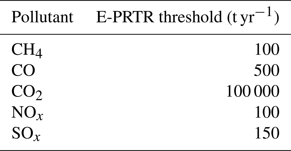
For European power plants, annual emissions were derived as a first step from the E-PRTR reporting in the E-PRTR_v18 and IRD v.7 databases. However, for many facilities, gaps in the E-PRTR emission reporting were identified and had to be corrected following a gap-filling routine (see below). The gaps are mainly due to the E-PRTR emission-reporting thresholds, which oblige companies to report emissions from individual pollutants only if they are above the values summarised in Table 2. Given the pollutant-specific reporting threshold for companies, many facilities report emissions for only a small number of pollutants. NO_x and CO₂ are the pollutants that are on average reported most often. CH₄ reporting is almost non-existent for power plants, while CO and SO_x are reported for a limited number of facilities, more often in the earlier years (2004–2010) and less so in recent years, when annual emissions may lie more often below the reporting threshold due to emission reduction technologies. Reporting for LCPs is not dependent on an emission threshold but is mandatory for all combustion plants with 50 MW or higher thermal input capacity, excluding ovens and certain types of chemical reactors. For each LCP, annual reporting of emissions of NO_x, SO_x, PM and fuel input by fuel type is required.

Table 2 Summary of the E-PRTR emission-reporting thresholds per pollutant.

To complete the reporting for all five pollutants, a five-step gap-filling routine was designed that follows several steps to estimate missing emission values for each power plant (Fig. 1).

1. In gap-filling step 1, the E-PRTR- and LCP-reported values are compared for those years in which reporting exists in both datasets for a specific plant. As the scope of an E-PRTR facility can be broader than just the LCPs at that location, the E-PRTR-reported emissions are typically similar to or higher than the LCP-reported emissions. If the correlation between both series is >0.5, it is assumed that the trends in the LCP-reported emissions are also representative of the trends in activity for the complete facility. In that case, the LCP value is used, multiplied by the average ratio between the E-PRTR- and LCP-reported emission values. In this way, if the EPRTR facility typically encompasses several smaller units that are not in the LCP dataset (i.e. <50 MW), the gap-filled emission value incorporates this relatively fixed ratio between E-PRTR and LCP emissions. The gap-filled emission value is capped at the highest reported emission value in the time series for this specific facility to limit the risk of gap filling unrealistic emission values. When the correlation is <0.5 but the aggregated ratio of the series total emissions is between 0.9 and 1.1, or if the median ratio between individual emission values for each year is between 0.9 and 1.1, the LCP value is used directly, as the two time series are considered to be sufficiently consistent, but no reliable adjustment ratio can be estimated.

2. In gap-filling step 2, when no E-PRTR reporting for a specific pollutant is available for any year or for none of the years where LCP reporting is available (which would allow a comparison), the LCP emission value is used directly when available, as this officially reported emission value is the most reliable estimate available and is assumed to be close to the total facility emissions in most cases.

3. After gap filling using LCP data, many gaps in the emission reporting remained. It was decided to fill the remaining gaps if emissions for at least one pollutant had been reported for the facility in a given year (implying that the facility was active). Gap-filling step 3 is performed by calculating the average ratios between reported CO₂ emissions and the reported emissions of other pollutants for the specific facility, as the facility-specific ratio between the fuel consumption and emission rates is assumed to be the most reliable relationship at this point. When specific pollutant emissions were missing but CO₂ emissions were available, the plant-specific ratio between CO₂ and the missing pollutant is used to estimate the missing emission. When fuel use information was not available, the use of pollutant ratios is also deemed the most appropriate method to gap fill missing CO₂ emissions. However, CO₂ is only gap-filled in this step when a NO_x value is reported, as this ratio is typically more stable than for the other co-emitted pollutants. Assuming the downward trend (e.g. lowering of the ${\mathrm{SO}}_x/{\mathrm{CO}}_{\mathrm{2}}$ ratio over time due to increased implementation of abatement technologies) of country-, fuel- and year-specific emission factors from the GAINS model, the emission ratios based on co-reporting in earlier years are adjusted before using them in later years to account for the effect of increasing use of abatement technologies.

4. In gap-filling step 4, missing emission values were gap-filled using the ratio between the IIASA GAINS model's implied emission factors (IIASA, 2018) (e.g. the ${\mathrm{CO}}_{\mathrm{2}}/\mathrm{CO}$ ratio) for a specific country, year, fuel type and pollutant applied to a CO₂ value established from E-PRTR reporting or gap-filling steps 1 or 2.

5. In gap-filling step 5, all the emission values that are still missing are gap-filled by applying the ratio between GAINS emission factors to values gap-filled in steps 3 or 4. For CH₄, a separate fuel-specific ${\mathrm{CO}}_{\mathrm{2}}/{\mathrm{CH}}_{\mathrm{4}}$ ratio is used to gap fill emission values based on the Tier 1 emission factors reported by the IPCC guidelines (Eggleston et al., 2006).

Figure 1 Illustrated example of gap filling E-PRTR missing emission values for facility X.

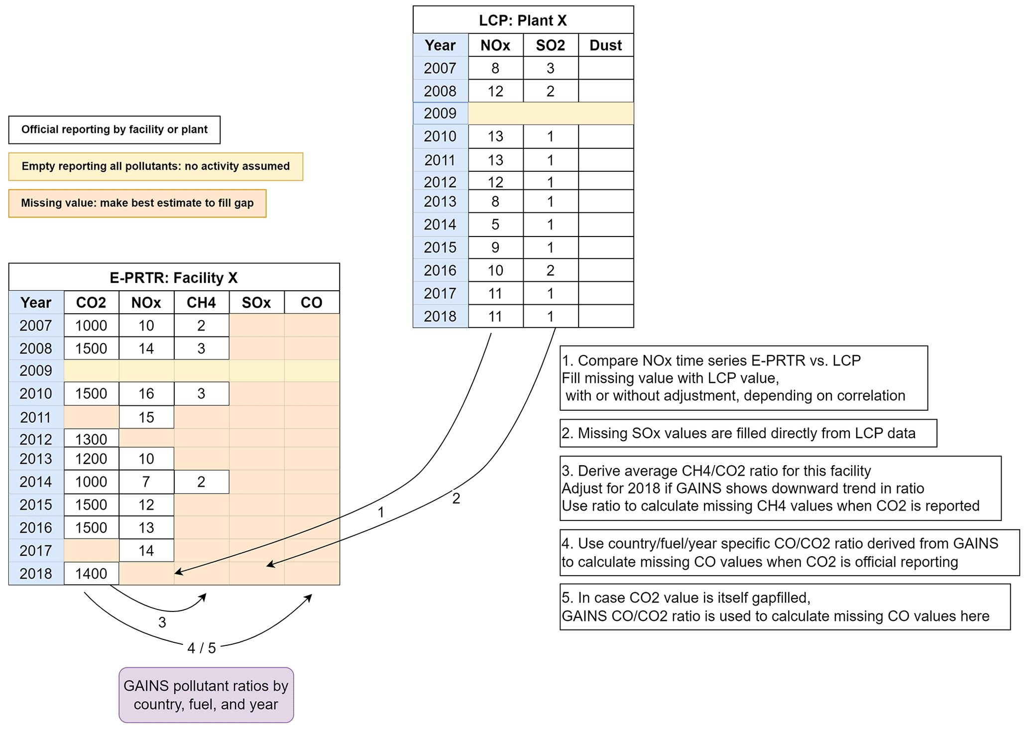
As the gap-filling steps progress, emission values filled by the later steps are typically more uncertain. To limit outlier values, gap-filled values derived from gap-filling steps 3 to 5 for all pollutants except CO₂ were capped at the E-PRTR reporting threshold value (thus following the assumption that the value was not originally reported due to it being below the reporting threshold).

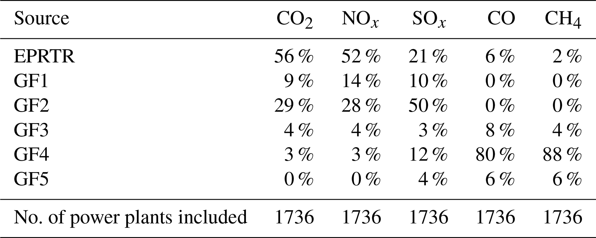
Table 3 shows what share of the final emission has been derived from E-PRTR reporting and the subsequent gap-filling steps (i.e. GF1 to GF5). The contribution of gap-filled emissions is most substantial for CO and CH₄, with more than 60 % of the total emissions from gap filling. Table 4 shows for which percentage of power plant locations the emission values have been gap-filled. From this perspective, gap filling plays a more prominent role, as the highest emission values have typically been reported and gap filling imputes mostly smaller emission values.

Table 3 Contributions of reported and gap-filled values to European power plant emissions in terms of total emissions (kt yr⁻¹).

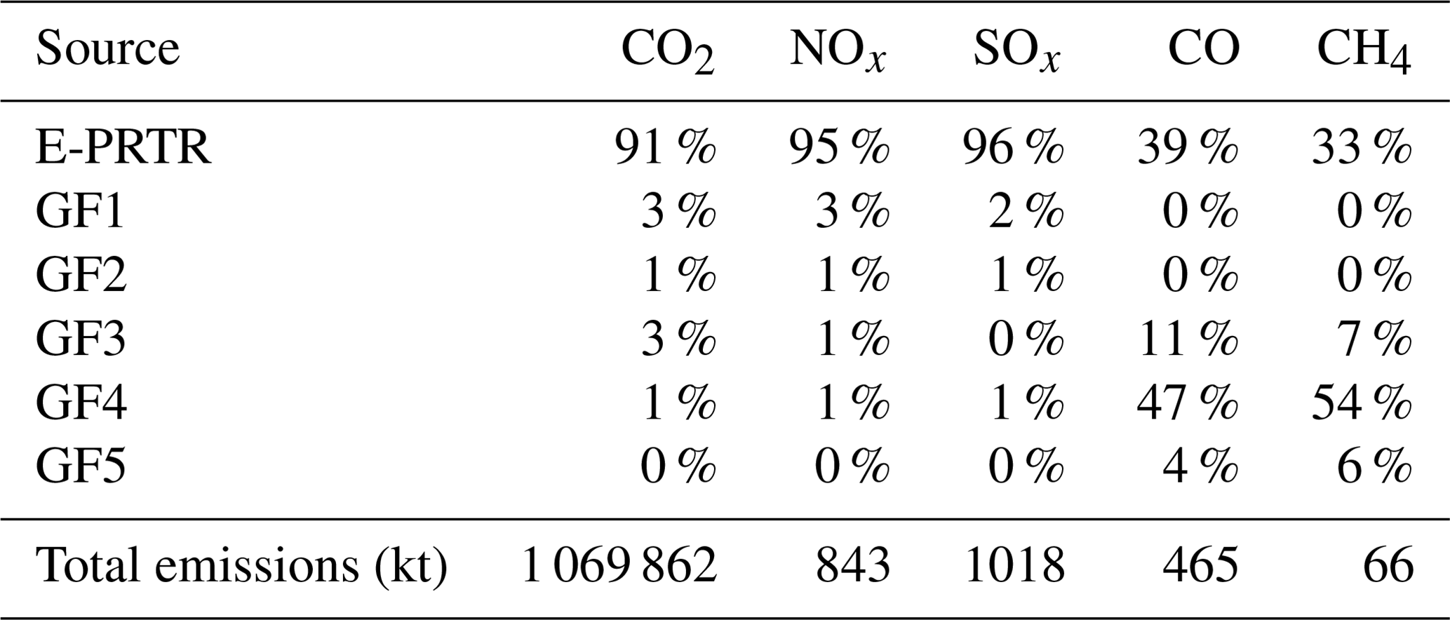
Table 4 Contributions of reported and gap-filled values to European power plant emissions in terms of the share of power plants.

2.3.2 Non-European countries

Plant-specific CO₂, NO_x, SO₂ and CH₄ emissions for all the US power plants were obtained from the eGRID database. Most emissions of CO₂, NO_x and SO₂ are taken from monitored data from the Clean Air Markets Division Power Sector Emission Data. For all other units and for CH₄, the reported emissions are based on measured heat input multiplied by an emission factor as described by the US EPA (2020). Emissions of CO, which are not reported by eGRID, were estimated using fuel-dependent average ratios between NO_x and CO emissions derived from the Continuous Emission Monitoring System (CEMS) database maintained by the Environmental Protection Agency (US EPA, 2021).

For the rest of the world, emissions per power plant were estimated following the steps below.

1. Estimation of CO₂ and CH₄ emissions per country, utility type (i.e. main or auto-producer plants) and fuel type combines the national energy statistics provided by the IEA World Energy Balances (IEA, 2021a) with the Tier 1 fuel-dependent emission factors reported by the IPCC guidelines (Eggleston et al., 2006).

2. Estimation of NO_x, SO₂ and CO emissions from coal-, natural-gas- and oil-fired power plants combines the CO₂ annual emissions estimated in step 1 with fuel-, country- or region-dependent average ratios between CO₂ emissions and emissions of other pollutants (e.g. the ${\mathrm{SO}}_{\mathrm{2}}/{\mathrm{CO}}_{\mathrm{2}}$ ratio) derived from the GAINS emission inventory (Amann et al., 2011; Klimont et al., 2017), which takes into account the heterogenous implementation of emission control restrictions in power plants across countries or regions. Emission ratios were constructed for a total of 23 non-EU countries or world regions, including China, India, South Africa, Japan and Australia. The ratios were estimated as an average of the emissions reported by GAINS for the years 2015 and 2020, since they are the closest to the reference year of our catalogue (2018). Figure 2 shows a comparison between the ${\mathrm{SO}}_{\mathrm{2}}/{\mathrm{CO}}_{\mathrm{2}}$ and ${\mathrm{NO}}_x/{\mathrm{CO}}_{\mathrm{2}}$ ratios for coal-fired power plants obtained for selected countries, indicating significant differences across them. The ${\mathrm{SO}}_{\mathrm{2}}/{\mathrm{CO}}_{\mathrm{2}}$ ratios estimated for Turkey and South Africa are approximately 17 and 10 times larger than the one estimated for China, the ratios reported for India and Australia also being considerably larger (i.e. between 5 and 7 times). The results are in line with differences across national emission legislation associated with the power generation industry. Emission standards for coal-fired power plants in China (200 mg m⁻³ for all existing plants and 35 mg m⁻³ for plants built after 2020) are much stricter than the ones established in Turkey (1000 mg m⁻³ in operation between 2004 and 2019), South Africa (680 mg m⁻³), India (600 mg m⁻³ for units commissioned before 2003, 200 mg m⁻³ for units commissioned between 2004 and 2016 and 100 mg m⁻³ for units installed after 2017) or Australia, where no national or state-wide limits exist. The estimated ${\mathrm{NO}}_x/{\mathrm{CO}}_{\mathrm{2}}$ ratios also vary across countries, China again being the country reporting the lower value. As for SO₂, NO_x emission limits for coal-fired power plants in China (100 mg m⁻³ for plants built from 2004 to 2011, 200 mg m⁻³ for plants built before 2004) are stricter than the ones implemented in South Africa (1020 mg m⁻³), Australia (856 mg m⁻³) and India (600 mg m⁻³ for units installed before 2003, 300 mg m⁻³ for units installed between 2004 and 2016 and 100 mg m⁻³ for units installed after 2017). The lower discrepancies among ${\mathrm{NO}}_x/{\mathrm{CO}}_{\mathrm{2}}$ ratios when compared to ${\mathrm{SO}}_{\mathrm{2}}/{\mathrm{CO}}_{\mathrm{2}}$ ratios indicate that, for SO₂, other elements than emission legislation may also play a role, such as the type and quality (e.g. sulfur content) of coal used in each country.

3. Estimation of NO_x, SO₂ and CO emissions from biomass- and waste-fired power plants combines the CO₂ annual emissions estimated in step 1 with fuel-dependent average ratios between CO₂ emissions and emissions of other pollutants (e.g. the ${\mathrm{SO}}_{\mathrm{2}}/{\mathrm{CO}}_{\mathrm{2}}$ ratio) reported by the E-PRTR-based European power plant database (see Sect. 2.3.1). The same ratios are assumed for all the countries due to the lack of more detailed information. Despite introducing some uncertainty, it is important to note that the contribution of these two fuels to the total combustion-related electricity generation is rather residual (less than 5 %; IEA, 2021a).

4. Estimation of CO emissions from biomass- and waste-fired power plants combines the NO_x annual emissions estimated in step 3 for these facilities with calculated fuel-dependent average ratios between NO_x and CO emissions derived from the US EPA CEMS database.

5. Estimated country- and fuel-dependent emissions derived from steps 1, 2, 3 and 4 are assigned to each facility as a function of the installed capacity and fuel information. The information on the installed capacity per power plant is provided by the databases described in Sect. 2.1.

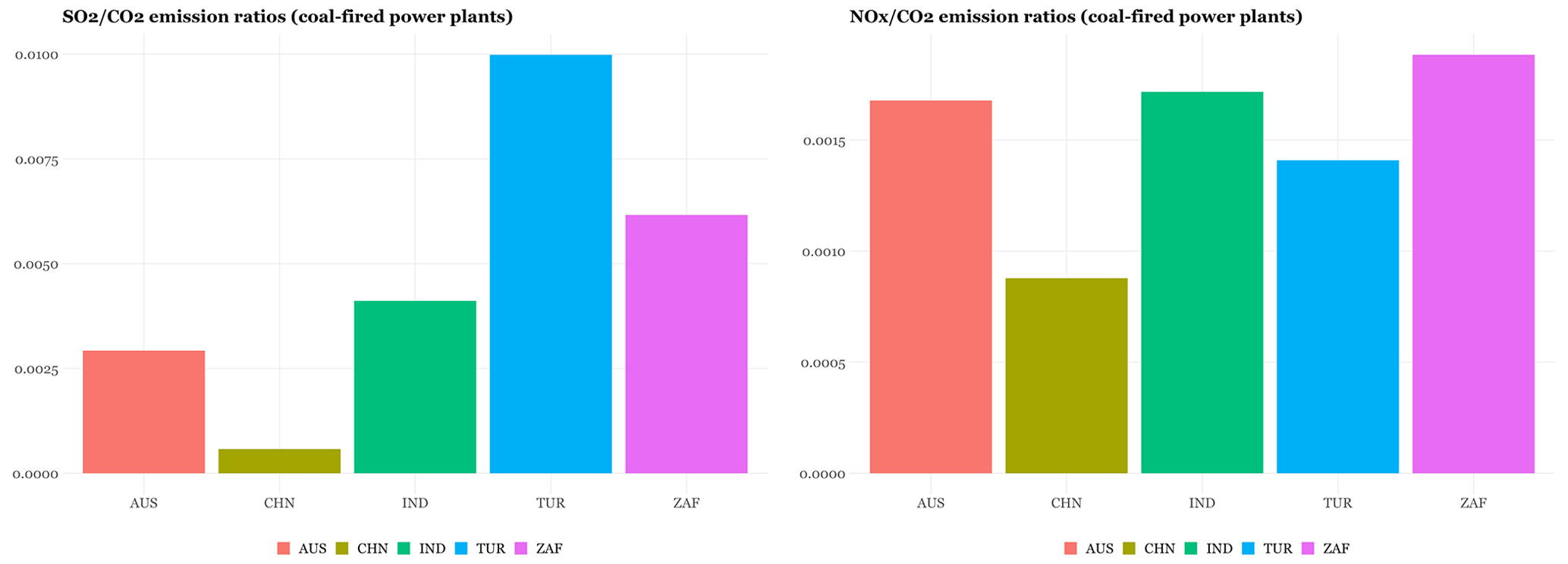
Figure 2 ${\mathrm{SO}}_{\mathrm{2}}/{\mathrm{CO}}_{\mathrm{2}}$ and ${\mathrm{NO}}_x/{\mathrm{CO}}_{\mathrm{2}}$ emission ratios for coal-fired power plants estimated for selected countries using the GAINS inventory (Amann et al., 2011; Klimont et al., 2017).

For coal-fired power plants we assumed that main and auto-producer facilities are correctly covered in all the countries, as the GCPTv2021_01 database reports both public and industrial facilities. On the other hand, emissions from auto-producer plants using oil, natural gas, biomass or waste were only considered in those countries where the difference between the total installed capacity (main producers plus auto-producers) reported by our database and the UN (2021) was lower than 10 %. For countries where this difference was larger than 10 %, we assumed that our database only covers the main activity producer plants, and therefore auto-producer emissions were excluded from the country-to-plant assignation process (step 4).

Figure 3 shows the relative differences between the total installed capacity reported by our database and the installed capacity reported by the UN (2021) for the main producers (red rectangles) and the main producers plus auto-producers (blue circles) for the top 50 non-European CO₂-emitting countries. For each country, the marker without the transparency effect indicates whether emissions from the main producers plus auto-producers (e.g. China, the USA, South Korea or Saudi Arabia) or only from the main producers (e.g. India, Russia, Japan or Iran) were considered.

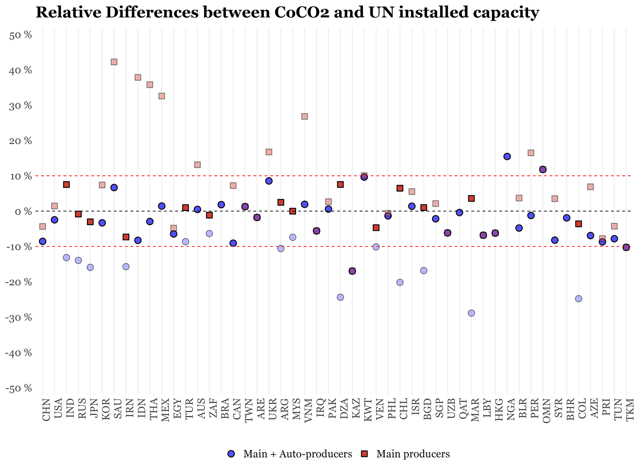
Figure 3 Relative differences (%) in the total installed capacity reported by the global point source database and the installed capacity reported by the UN (2021) for the main producers (red rectangles) and the main producers plus auto-producers (blue circles) for the top 50 non-European CO₂-emitting countries. For each country, the marker without the transparency effect indicates whether emissions from the main producers plus auto-producers or only from the main producers were considered.

Overall, we could not include emissions from the auto-producers in 35 % of the countries considered. This translates to 4.1 % of the total estimated CO₂ emissions from the power sector that could not be allocated to the final non-European point source database due to the lack of information from auto-producers. Figure 4 represents the share of the total national CO₂ emissions that could not be allocated per country. It is observed that most of the countries where information on auto-producers could not be found are in South America and Africa. Benin, El Salvador, Mali, Ecuador, Costa Rica and Madagascar are among the countries where the largest share of total CO₂ emissions remained unallocated (between 70 % and 50 %). Emissions from these countries are however not significant, and therefore they have a very limited impact on the overall non-allocated emissions. In high-emitting countries such as Russia, India or Japan, the share of national emissions that could not be assigned to individual facilities is much lower (i.e. 14 % to 21 %).

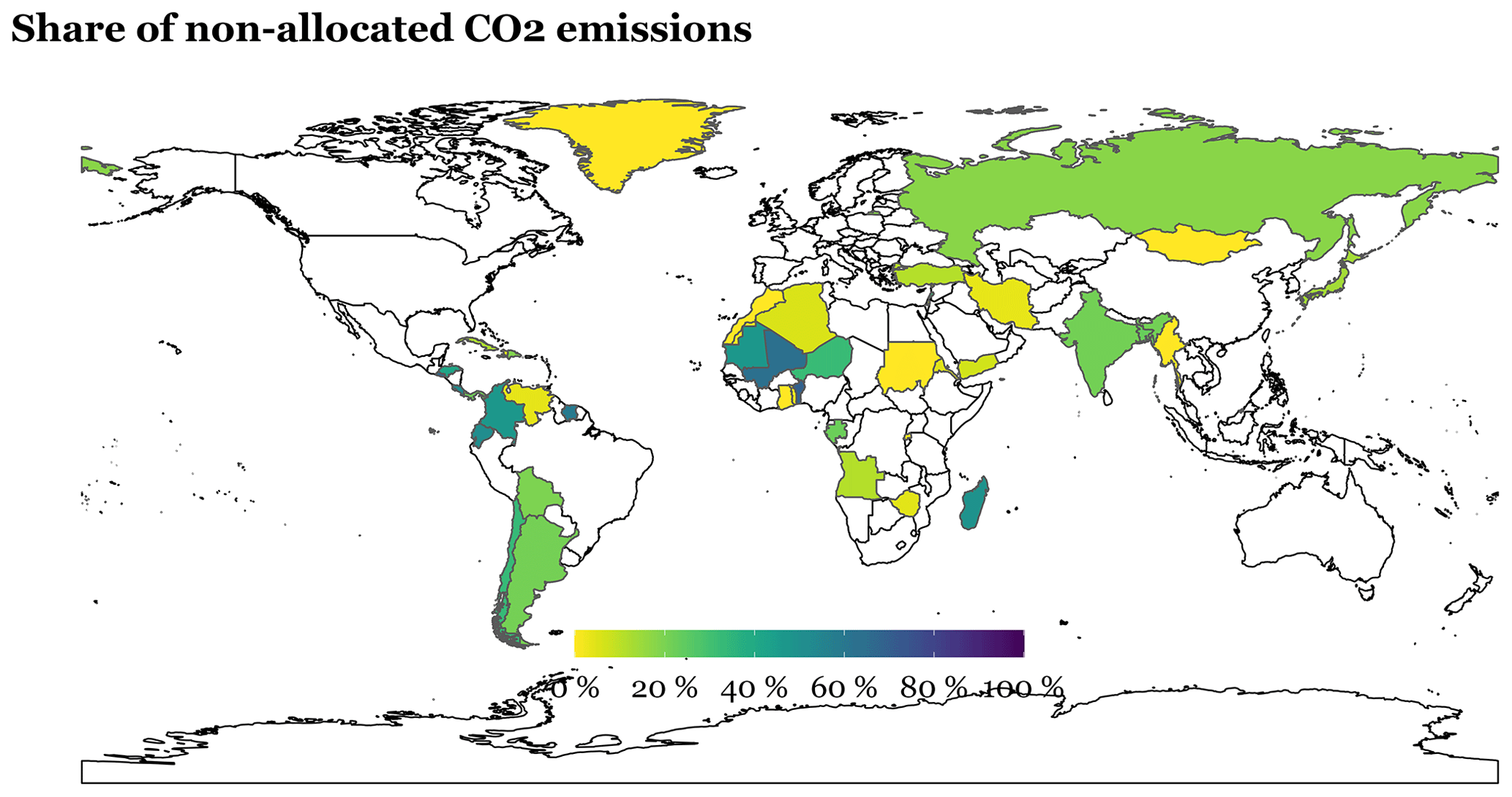
Figure 4 Share of total national CO₂ emissions (%) from the power sector that could not be allocated due to the lack of information from auto-producers. Countries where emissions from the main producers and auto-producers could be allocated are represented in white.

2.4 Temporal profiles

Country-dependent (state-dependent for the USA) and fuel-dependent monthly, weekly and hourly temporal profiles were constructed for all the power plants (i.e. European and non-European datasets) using the electricity production statistics summarised in Table 5. For countries where electricity generation statistics are not disaggregated by fuel type, we assumed the same temporal distribution for all types of power plants. For countries with no information on electricity generation or with information only available at e.g. the monthly scale but not at the hourly scale, averaged profiles from countries belonging to the same world region were used. The definition of world regions was taken from the EDGARv5 emission inventory (Crippa et al., 2018). The resulting profiles were assigned to each facility as a function of the country and fuel type information.

Table 5 Sources of electricity production statistics and corresponding characteristics.

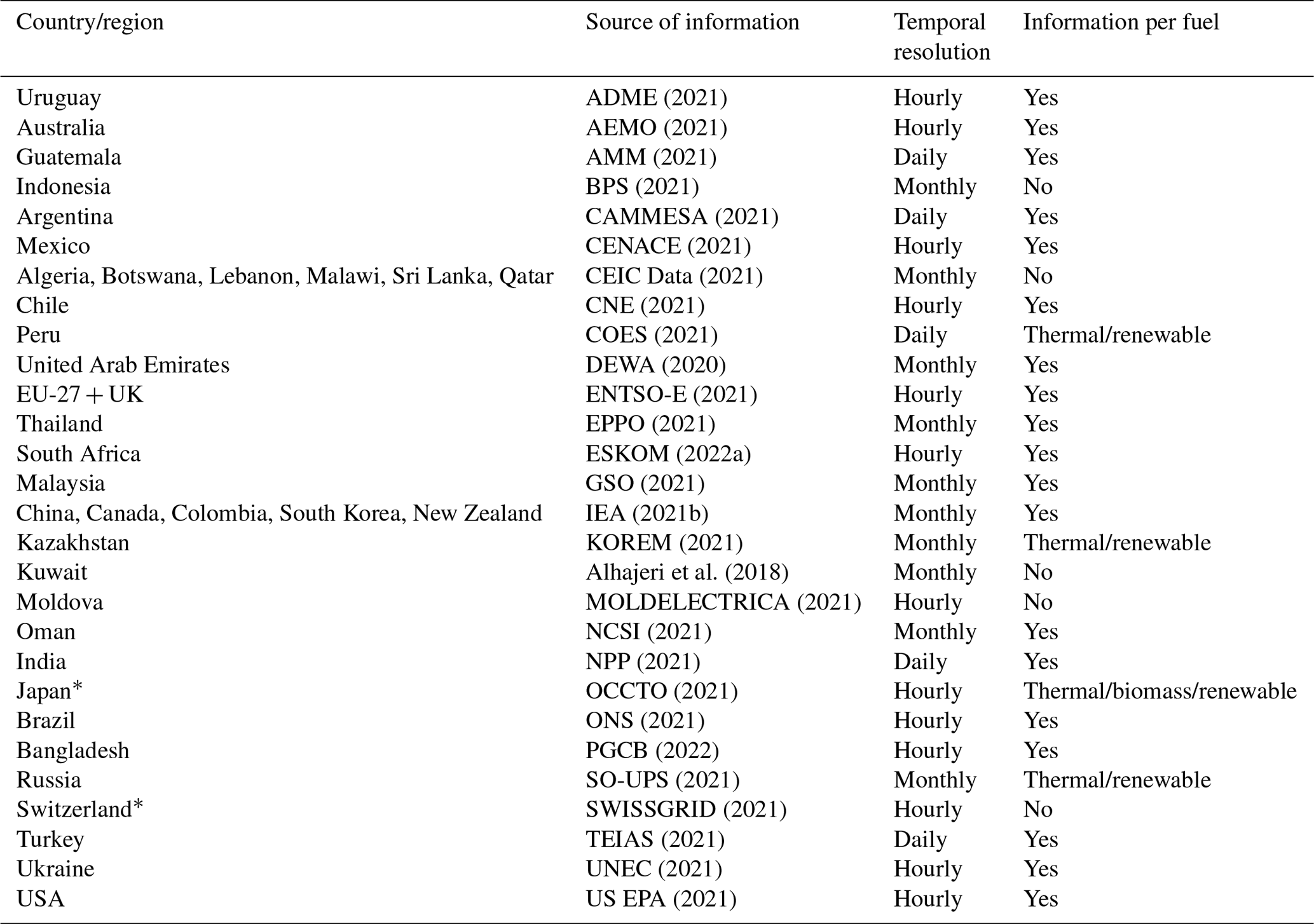
^∗ Monthly data derived from the IEA as reported by fuel type.

Figure 5 illustrates, on the one hand, the countries for which specific monthly, weekly and hourly profiles were constructed based on the statistics compiled and, on the other hand, the resulting share of total CO₂ emissions for which specific monthly, weekly and hourly profiles were available. For the monthly profiles, the database constructed covers a total of 96 countries plus 42 USA states, which translates to more than 90 % of the total CO₂ emissions from the power sector. For weekly and hourly profiles, the coverage in terms of total CO₂ emissions is much lower (approximately 46 % and 36 %, respectively), partially because no information on electricity production at the daily and hourly levels was available for China. For this country, we assumed that the weekly cycle of emissions follows the pattern obtained for India, which shows no significant difference between weekdays and weekends. This assumption is in line with the results found by Wu et al. (2022) in which weekly profiles for Chinese power plants were constructed using measured emissions derived from continuous emission monitoring systems.

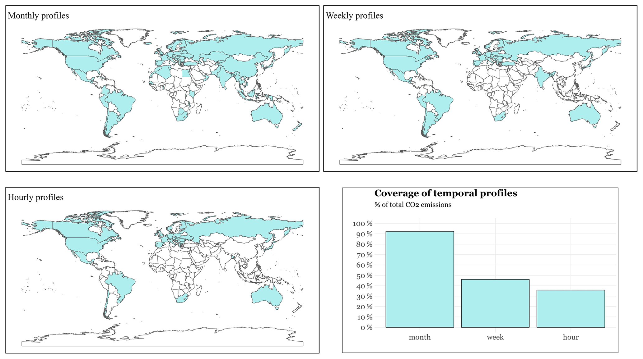
Figure 5 Spatial coverage of the constructed monthly, weekly and hourly temporal profile databases. Share of total CO₂ emissions (%) from the power sector for which specific monthly, weekly and hourly profiles were developed.

2.5 Vertical profiles

Hourly effective emission heights at the facility level were simulated by combining 2018 global hourly gridded meteorological information (i.e. air temperature at stack height, wind speed at stack height, surface temperature, boundary-layer height, friction velocity and Obukhov length) simulated by the Multiscale Online Nonhydrostatic AtmospheRe CHemistry model (MONARCH) at 0.3×0.3^∘ (Badia et al., 2017) with facility-level stack parameter information (i.e. height, diameter, exit velocity and exit temperature). Information on stack parameters was obtained from the following sources.

• The point source database of electric generation units (PTEGUs), obtained from the US EPA emission modelling platform (US EPA, 2021), which reports plant-level stack parameter information for US power plants.

• The HERMES Spanish power plant database (Guevara et al., 2013)

• Atmospheric emission licenses of South African power plants (CER, 2022)

• The list of the tallest chimneys worldwide reported by Wikipedia (2022a)

• The list of the tallest chimneys in Poland reported by Wikipedia (2022b)

• The list of the tallest chimneys in the Czech Republic reported by Wikipedia (2022c)

• The list of the tallest structures in Germany reported by Wikiwand (2022)

The Indian Ministry of Environment, Forest and Climate Change (MoEFCC, 2015) requires all coal-fired power plants with a generation capacity of 500 MW and above to build a stack of minimum height 275 m, those with between 210 and 500 MW to build a stack of minimum height 220 m, and those with less than 210 MW to build a stack based on the estimated SO₂ emission rate (Q; kg h⁻¹) and a rule of thumb of height $=\mathrm{14}\cdot \left(Q\right)\mathrm{0.3}$. Considering this information, we assumed that all coal-fired power plants in India with a generation capacity of 500 MW and above had a stack height of 275 m and that those with between 210 and 500 MW had a stack height of 220 m.

In some European coal-fired power plants built in recent years, which must be equipped with a flue gas cleaning system, the cooling tower also takes on the function of the chimney. The original chimneys were dismantled, and now emissions are released through the cooling towers, which have different stack conditions. For Germany, we identified the list of power plants with cooling towers used as chimneys and the associated stack heights through Wikipedia (2022d), and we completed the information with the stack diameter, exit temperature and exit velocity reported by Brunner et al. (2019). This level of detail is not considered in facilities from other countries due to a lack of information.

Fuel-dependent and CO₂-emission-weighted average stack parameters were calculated using the PTEGU dataset and assigned to all those facilities for which no specific information was found. For waste-to-energy power plants, we considered the stack parameters reported by Pregger and Friedrich (2009) as the PTEGU dataset does not include this type of facility. Table 6 summarises the stack parameters proposed per fuel type and the associated number of units considered to calculate the values.

Table 6 Fuel-dependent and CO₂-emission-weighted average stack parameters assigned to facilities with no specific information and number of sources considered to calculate them.

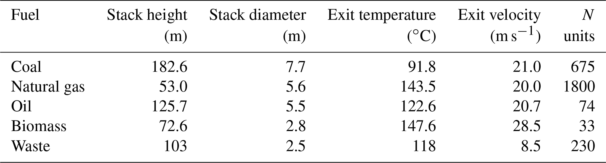
Figure 6 illustrates, on the one hand, the facilities assigned specific (red circles) or emission-weighted averaged (white circles) stack height information and, on the other hand, the share of the total CO₂ emissions from the power sector assigned specific stack parameter information. In terms of emission coverage, only 28 % of the total CO₂ emissions from the power sector are assigned specific stack height values. This share significantly varies across world regions. In the USA, South Africa and India the share is between 75 % and 90 %, while in central Europe it is around 50 %. In many Asian, African and South American regions the share is below 5 %. The coverage of total CO₂ emissions for stack diameter, exit velocity and temperature is even lower than for the stack height parameter (i.e. approximately 15 % globally in all the cases), the differences between regions being equally heterogeneous. These results indicate the current lack of stack parameter information.

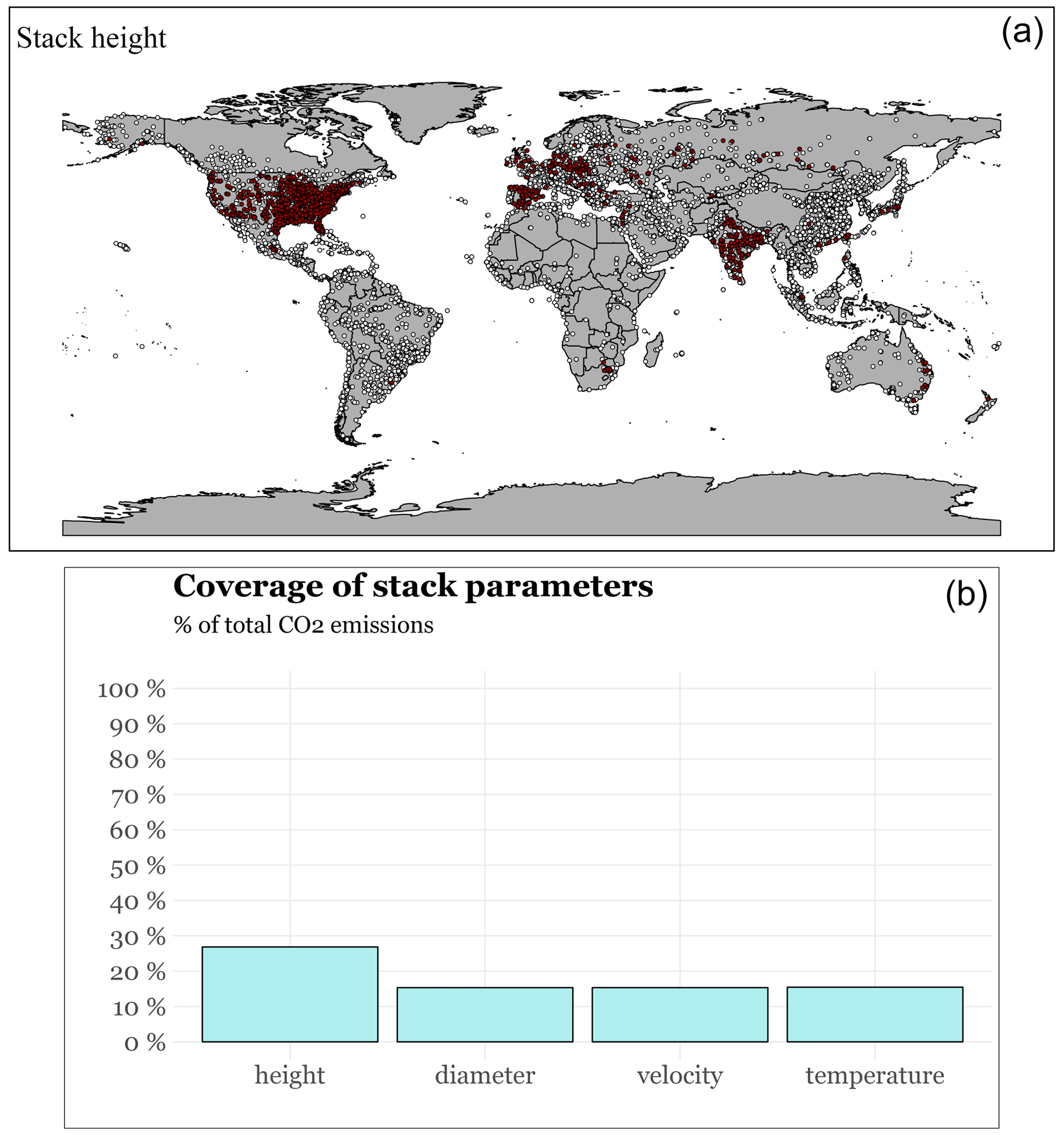
Figure 6 Facilities assigned specific (red circles) or emission-weighted averaged (white circles) stack height information (a) and the share of total CO₂ emissions (%) from the power sector for which specific stack parameters (height, diameter, exit velocity and exit temperature) were assigned (b).

The plume rise calculations at the hourly and facility level were performed using the High-Elective Resolution Modelling Emission System version 3 (HERMESv3) bottom-up emission system (Guevara et al., 2020), which includes plume rise formulas as described by Gordon et al. (2018). The HERMESv3 system was used to break down facility-level annual emissions into hourly resolution using of the temporal profiles described in Sect. 2.4 and to estimate hourly effective emission heights per plant considering the meteorological information provided by the nearest grid cell of MONARCH. Hourly plume top and plume bottom values per facility (h_top(h,f), h_bot(h,f)) were derived from the estimated effective emission heights following the expressions reported by Bieser et al. (2011) (Eqs. 1 and 2):

$$\begin{array}{}\text{(1)}& {\displaystyle }{h}_{\mathrm{top}}\left(h,f\right)=h_{\mathrm{s}}\left(f\right)+\mathrm{1.5}\cdot \mathrm{\Delta }h(h,f),\text{(2)}& {\displaystyle }{h}_{\mathrm{bot}}\left(h,f\right)=h_{\mathrm{s}}\left(f\right)+\mathrm{0.5}\cdot \mathrm{\Delta }h(h,f),\end{array}$$

where h_s(f) is the stack height of the facility f and Δh(h,f) is the modelled effective emission height for the facility f and hour h.

3 Results

3.1 Annual emissions

Figures 7 and 8 show the plant-level CO₂ and NO_x annual emissions as reported by the resulting global point source database. Results are distinguished by fuel type. It is observed that coal-fired power plants (red circles) are the main contributors to the total CO₂ emissions, the top emitters being in China, India, the USA, Australia, South Africa, central Europe and Indonesia. CO₂ emissions from natural gas power plants (blue circles) are dominant in Russia and some countries from the Middle East (e.g. Saudi Arabia and Iran). For NO_x, the main contributors are also coal-fired power plants, but several oil-fired power plants (black circles) gain importance when compared to their contributions to the CO₂ emission map, especially in the Middle East (i.e. Iran and Saudi Arabia), Indonesia, Venezuela and some countries in northern Africa. In China, India, the USA, Australia, South Africa and central Europe, NO_x emissions are mainly dominated by coal-fired power plants. For both pollutants it is observed that the number of high emitters in Africa and South America is rather scarce, expect for South Africa and some countries in northern Africa as well as Venezuela. This is related to the fact that in both regions the electricity production is mainly dominated by renewable sources (e.g. hydro, solar) (IEA, 2021a). Linked to this aspect, it is interesting to see the large number of biomass power plants in Brazil (brown circles), as this fuel represents the second largest energy source in the country, just behind hydropower. A significant number of waste-to-energy plants (green circles) is reported in Japan and China, the two countries with the largest installed incineration capacity (Lu et al., 2017).

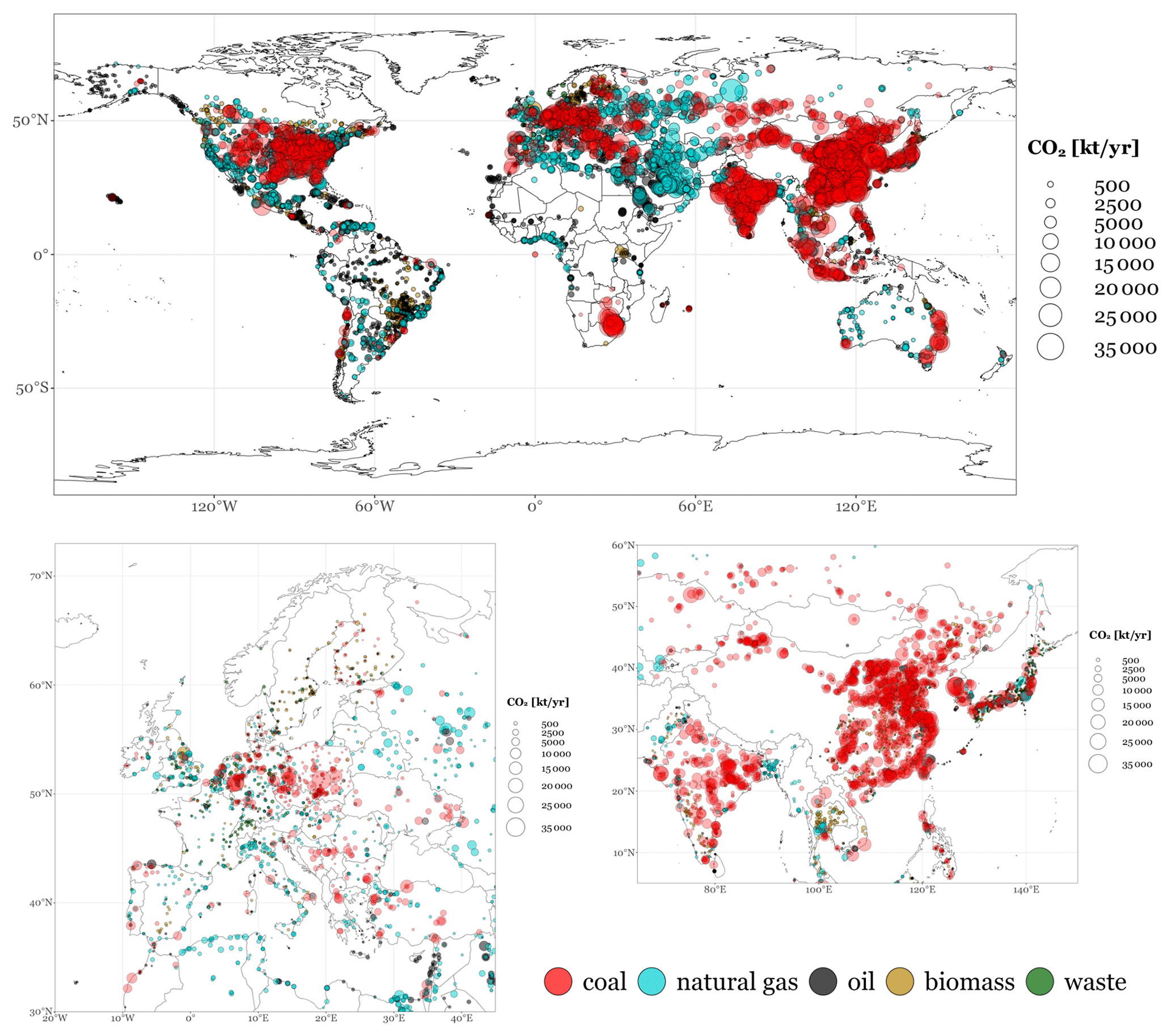
Figure 7 Plant-level CO₂ annual emissions (kt yr⁻¹) as reported by the resulting global point source database, including zooms over Europe and Asia. Emissions are colour-classified according to the main fuel used: coal (red), natural gas (blue), oil (black), waste (green) and biomass (brown).

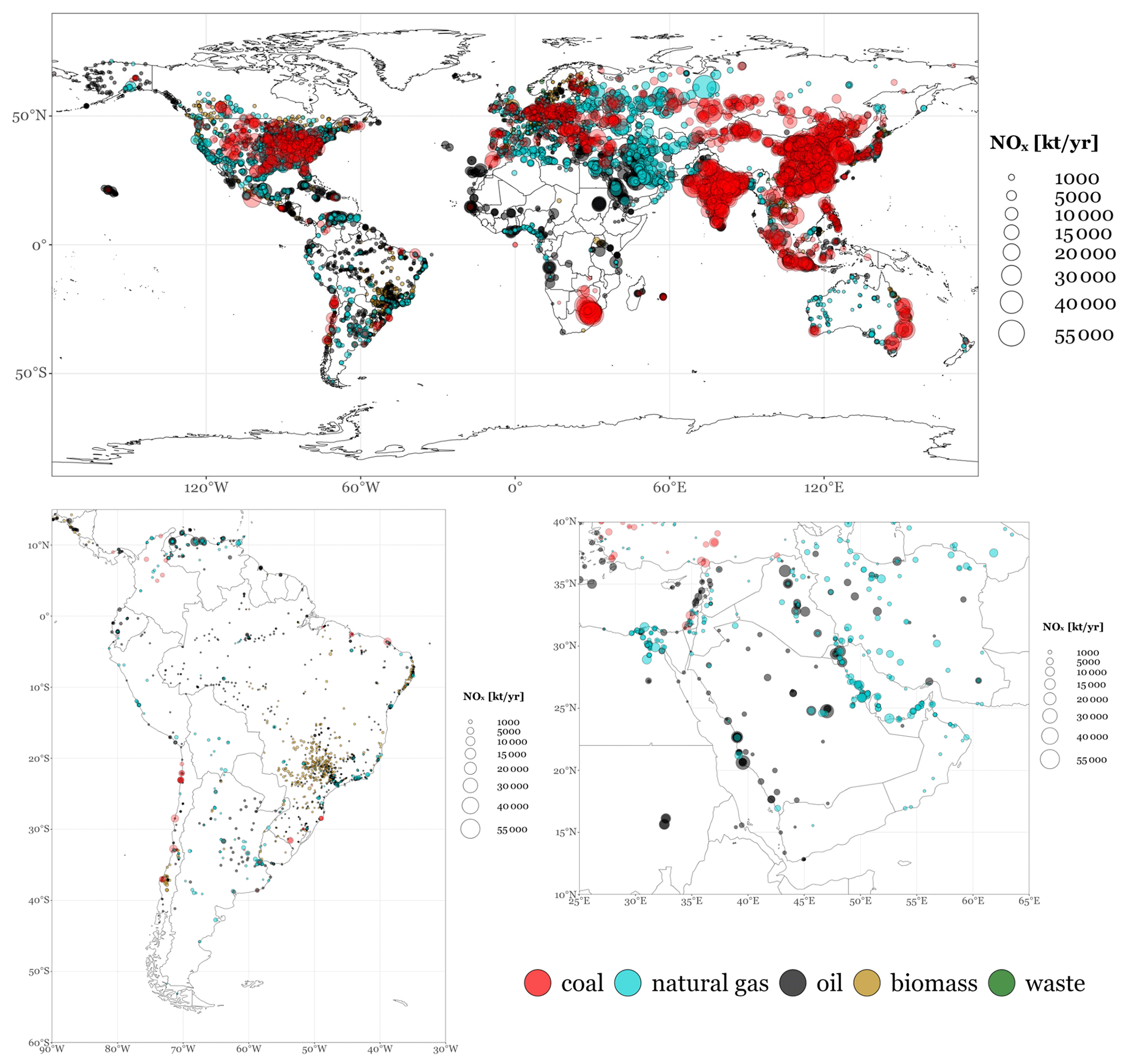
Figure 8 Plant-level NO_x annual emissions (kt yr⁻¹) as reported by the resulting global point source database, including zooms over South America and the Middle East. Emissions are colour-coded according to the main fuel used: coal (red), natural gas (blue), oil (black), waste (green) and biomass (brown).

Tables 7 and 8 list the top 15 CO₂- and NO_x-emitting power plants worldwide and in EU-27 + UK.

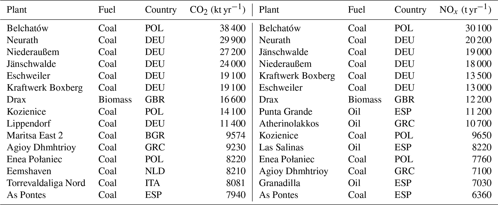
At the global level, the Belchatów (Poland), Taean (South Korea), Taichung (Taiwan), Dangjin (South Korea) and Datang Tuoketuo (China) power plants are the top five CO₂ emitters. These five facilities are also the five largest coal-fired power stations in the world (with installed capacities between 6700 and 5300 MW). All top 15 CO₂ emitters are coal-fired power plants, except for Surgutskaya GRES-2 (Russia), which is the largest combined-cycle natural-gas-fired power station of Russia (8865 MW) and supplies energy to nearly 40 % of the population. Most of the top 15 CO₂ emitters are in Asian countries, including South Korea (3), China (2), Taiwan (2), Malaysia (2), India (1) and Kazakhstan (1), while the rest are in Europe: Germany (2), Poland (1) and Russia (1). Seven out of the top 10 emitters identified in this work are also listed in the 2018 top 10 CO₂-polluting power plants reported by Grant et al. (2021). In EU-27 + UK, it is observed that most of the 15 top CO₂ emitters are in Germany (6) and Poland (3). Similarly to what is observed at the global scale, 14 out of the 15 facilities are coal-fired power plants, the remaining worst polluter being the Drax biomass power station, the largest power plant in the UK (3906 MW) that is also capable of co-firing petroleum coke. The largest emitter in EU-27 + UK (Belchatów, Poland) reports almost 5 times more CO₂ emissions than the 15th facility (As Pontes, Spain).

For NO_x, the list of top emitters mainly consists of coal-fired power plants (14 out of 15). Seven of these plants appear in both the CO₂ and NO_x top 15 emitter lists, including Surgutskaya GRES-2 (Russia), Taean (South Korea), Dangjin (South Korea), Manjung (Malaysia), Yeongheun (South Korea), Ekibastuz-1 (Kazakhstan) and Vindhyachal (India). Concerning the other top 15 emitters, 6 of them are located in South Africa and 2 in India. At the EU-27 + UK level, Belchatów is again the largest emitter. Four out of the top five emitters are in Germany, all of them being coal-fired power plants. There are also four Spanish facilities, three of them being oil-fired internal combustion engines located in the Canary Islands. The other non-coal facilities that complete the European top 15 list are Drax (UK) and Atherinolakkos (Greece), the latter also being operated with diesel engine units. Additional information on the total emissions obtained at the country level is provided in Sect. 3.2.

Table 7 List of the top 15 CO₂-emitting (kt yr⁻¹) and NO_x-emitting (t yr⁻¹) power plants worldwide.

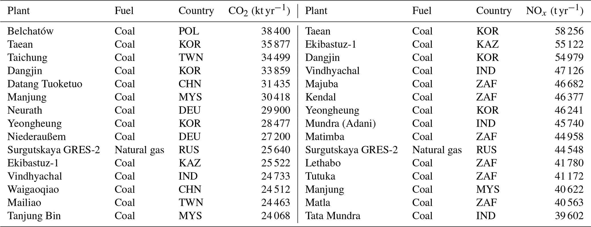
Table 8 List of the top 15 CO₂-emitting (kt yr⁻¹) and NO_x-emitting (t yr⁻¹) power plants in EU-27 + UK.

3.2 Comparison with independent inventories

The estimated annual emissions were compared against other independent plant- and country-level inventories. The following sub-sections present and discuss the results.

3.2.1 Plant level

Estimated plant-level emissions were compared against information reported by the CARMAv3 global database. As mentioned in Sect. 1, and despite no longer being maintained, the CARMAv3 database is still used as a proxy for the spatial representation of power plant emissions in several state-of-the-art inventories and modelling systems, like the EDGAR inventory (Janssens-Maenhout et al., 2019) and the Carbon Cycle Fossil Fuel Data Assimilation System (CCFFDAS) (Asefi-Najafabady et al., 2014).

Table 9 summarises the comparison between the total number of power plants and associated CO₂ emissions reported by CARMAv3 and this work for selected countries, including China, the United States, India, Germany, South Korea, South Africa, Australia, Taiwan and Poland. For China the present work reports 79 % more facilities and 92 % more emissions than CARMAv3. This result is in line with the fact that CARMAv3 was built using information from 2009, and during the last decade the number of power plants in China and the associated emissions have significantly increased (IEA, 2023). For the USA, the number of plants reported by each database is almost the same (−1 %), but emissions are lower in this work when compared to CARMAv3 (−17 %). This difference is mainly related to the transition from coal to natural gas and renewables that occurred during the last decade (EIA, 2021). Greenhouse gas emissions for electricity generation from natural gas are generally lower than those from oil and coal due to a more beneficial heat per carbon density and higher combustion efficiencies (e.g. IPCC, 2011). For Germany, South Africa, Poland and Australia it is observed that, despite including fewer facilities (differences between −47 % and −63 %), the total CO₂ emissions reported by this work are generally in line with CARMAv3 values (differences between −12 % and 0 %). This is because CARMAv3 is mostly based on Platts WEPP (Platts, 2015), which contains many small-sized auto-producer units (e.g. boilers located in commercial and institutional buildings such as hospitals or airports) with very low emission levels associated with them that are not considered in the present work. Moreover, and as shown below, CARMAv3 includes power plants that are not currently operating as they were shut down during the last decade. For India the present catalogue reports 81 % more emissions than CARMAv3 despite including −30 % fewer facilities, which indicates that the additional plants considered in CARMAv3 are low-level emission small plants. This hypothesis is confirmed when comparing the median CO₂ annual emission values of each dataset, the one reported by the present catalogue (154 669 kt CO₂ yr⁻¹) being almost 18 times larger than CARMAv3 (8839 kt CO₂ yr⁻¹). Differences between the present database and CARMAv3 are also linked to the fact that emissions reported by CARMAv3 exclude CO₂ from biofuels, while the present catalogue includes solid-biomass-fired power plants.

Table 9 Comparison between the total number of facilities and associated CO₂ emissions (kt yr⁻¹) reported by CARMAv3 and this work for the selected countries (China, the United States, India, Germany, South Korea, South Africa, Australia, Taiwan and Poland.

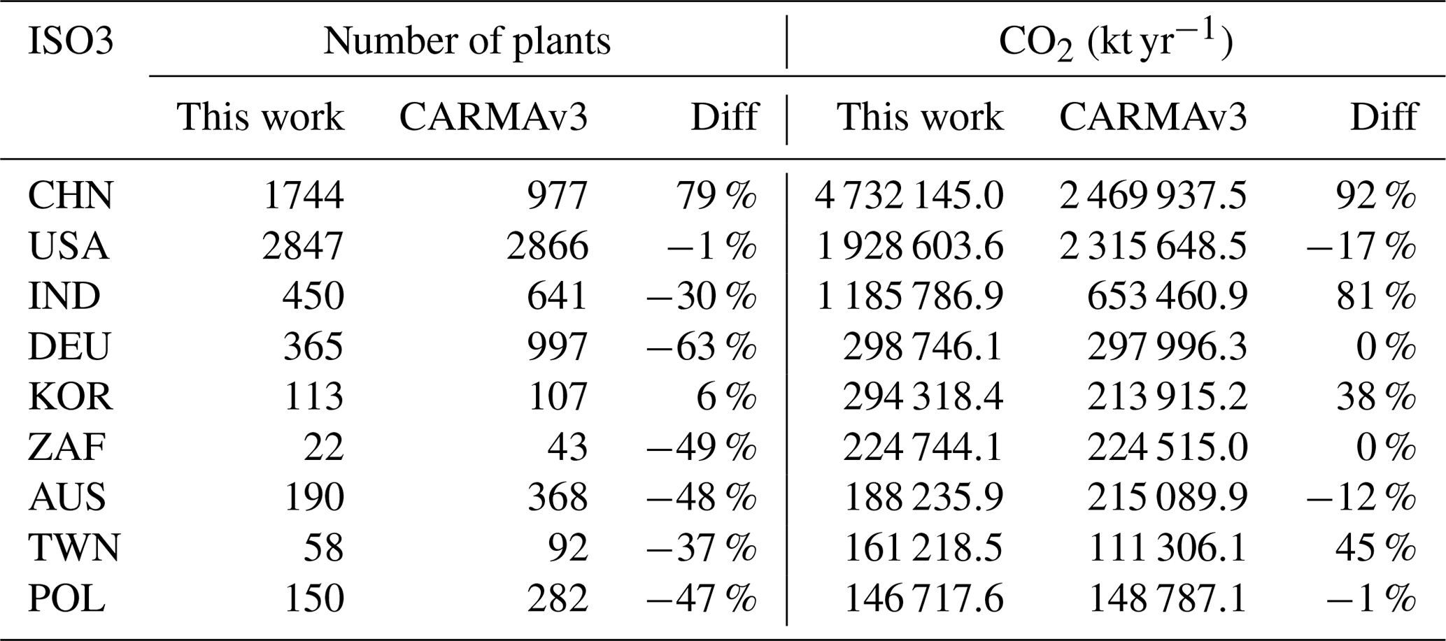
Figure 9 shows a plant-to-plant comparison between the top 20 emitters reported by this work and CARMAv3 for selected countries (i.e. United States, Taiwan, South Africa and Poland). In all of them it is observed that CARMAv3 reports emissions for plants that are not included in the present catalogue as they are currently retired or not operating (e.g. Jenwu power station in Taiwan or Adamow power station in Poland). Except for the case of the United States (i.e. the Monticello Steam Electric Station), most of these plants were already reporting low emissions in 2009, which could indicate that they were already in the process of being disconnected from the grid. The good agreement in South Africa, Poland and Taiwan (R² between 0.86 and 0.97) indicates that the levels of emissions from the top emitters in these countries remained stable between 2009 and 2018 (e.g. Kendal Power Station in South Africa or Belchatów power station in Poland). By contrast, significant discrepancies are observed in the United States (R²=0.41), the results reported by this work being consistently lower than CARMAv3 for all the top emitters. As mentioned before, these differences are mainly driven by the reduction in the rate of utilisation of coal-fired power plants and the conversion of coal-fired plants to natural gas during the last decade. Note that, for most of the emissions in the USA (99 %), the European Union (63 %), Canada (96 %), India (78 %) and South Africa (91 %), the plant-level CO₂ reported by CARMAv3 was directly obtained from official disclosure databases such as E-PRTR or the US EPA Clean Air Markets, which are also considered in the present work, while for the rest of the countries plant-level emissions were computed considering estimated key variables (i.e. capacity factor, heat rate and CO₂ emission factors) using statistical models fitted to a detailed dataset of US facilities (Wheeler and Ummel, 2008). This emission estimation approach is substantially different from the one considered in the present work (see Sect. 2.3.2) and could also contribute to the discrepancies obtained between the datasets besides the differences in the year of reference mentioned above.

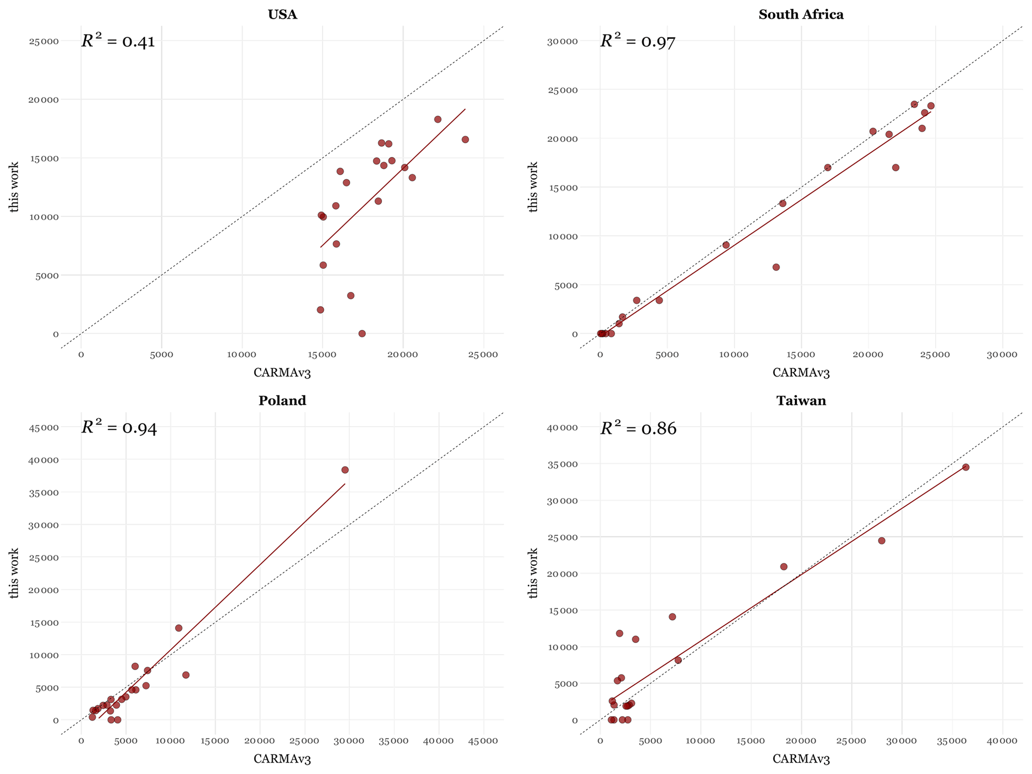
Figure 9 Plant-to-plant CO₂ annual emission comparison between the top 20 emitters reported by this work and CARMAv3 for the United States, Taiwan, South Africa and Poland (the dashed line represents the 1:1 line).

Besides comparing total annual emissions, we also compared the geographical location reported by the present catalogue and CARMAv3 for each of the top 20 emitters in the nine countries listed in Table 9. We found six facilities in which the location reported by CARMAv3 was off by hundreds of kilometres (between 120 and 337 km), while in 24 cases the locations provided by CARMAv3 were displaced from the right coordinates by tens of kilometres (between 11 and 79 km). Most of these cases (22 out of 30) correspond to units in Asia (i.e. China, Taiwan and India) where the wrongly allocated CARMAv3 power plants tend to be assigned to nearby city centres (Fig. S1). The differences between the locations reported in this work and CARMAv3 are much lower when looking at European (Polish and German) and US facilities, where the average distance between the geographical coordinates reported by each dataset is approximately 600 m and the maximum discrepancy is 5.7 km. These findings are consistent with the methods used in CARMA to add geographic data to the power plants. For about 70 % of the CARMAv3 power plants, the geocoding is performed using an algorithm that derives city-centre latitude and longitude coordinates from the geopolitical data (i.e. country, state, province and city names) provided by WEPP. On the other hand, for the facilities located in Europe, the USA and Canada (approximately 6000), exact geographical coordinates were obtained from high-resolution disclosure databases and manual geocoding. The geographical dislocation of the CARMAv3 facilities described here for Asia is consistent with other recent investigations (e.g. Zhang et al., 2022).

Figure 10 shows a comparison between the plant-level CO₂ and annual emissions (kt yr⁻¹) estimated by this work and reported by the GIDv1.1 database. Results are shown for the top 50 emitters reported by each inventory (a total of 76 facilities). Overall, the total emissions are almost equal (differences of −0.3 %). However, important discrepancies are observed at the plant level. In 41 of the 76 facilities, the differences between the reported annual CO₂ emissions are in the range ±25 %, with larger discrepancies being observed for the rest of the power plants. The CO₂ emissions estimated for the Bełchatów coal-fired power plant (Poland) in this work (38 400 kt yr⁻¹) are 2.75 times larger than the results reported by GIDv1.1 (14 051 kt yr⁻¹). The emissions estimated in this work are in line with the results reported by Grant et al. (2021) for the same facility (i.e. 37 600 kt yr⁻¹), both studies suggesting that Bełchatów is the top CO₂ emitter worldwide. Important discrepancies are also observed in several German coal-fired power plants (i.e. Niederaußem, Neurath, Weisweiler, Kraftwerk Boxberg and Jänschwalde), in which the emissions reported by this work are between 2 and 2.6 times larger than the GIDv1.1 results. Parts of these discrepancies are probably related to the fact that the GIDv1.1 inventory is based on 2019 activity data, while the present work considers 2018 as a reference year. Despite differing by only 1 year, quick decarbonisation efforts may be playing an important role in the resulting emissions. Following with the example of Germany, the total amount of coal used in this country to produce electricity decreased by −24 % between 2018 and 2019 (IEA, 2023). This fact is in line with the results reported by the integrated Industrial Reporting Database v.7 (EEA, 2022), which indicates that CO₂ emissions in the Niederaußem, Neurath and Jänschwalde coal-fired power plants were 1.4 times larger in 2018 when compared to 2019. The CO₂ emissions reported for Niederaußem by this work coincide with the value estimated by Grant et al. (2021) (27 200 kt yr⁻¹).

The result of this comparison also shows power plants for which the emissions estimated by this work are much lower than the results reported by GIDv1.1. This is the case, for instance, for the Rajiv Gandhi coal-fired (India) and Shin Sakaiko liquefied natural-gas-fired (Japan) power plants, where emissions are 0.3 and 0.15 times the ones reported by GIDv1.1. For the Rajiv Gandhi coal-fired power plant, the results reported by this work (6235 kt yr⁻¹) are larger than the facility-level emissions reported by the Central Electricity Authority (3557 kt yr⁻¹; CEA, 2022), indicating that GIDv1.1 (19 979 kt yr⁻¹) may be overestimating the emissions in this facility. Concerning the Shin Sakaiko power plant, no independent values could be found to compare against the results estimated by this work and GIDv1.1. However, and based on the information of the installed capacity, we hypothesise that GIDv1.1 emissions reported for this plant are also overestimated. According to GIDv1.1, the Shin Sakaiko power plant is the 14th highest CO₂ emitter worldwide despite having an installed capacity of 2000 MW, which is more than 2 times lower than the capacity of the Futtsu power plant (5040 MW), the first (fourth) largest gas-fired power station in Japan (the world).

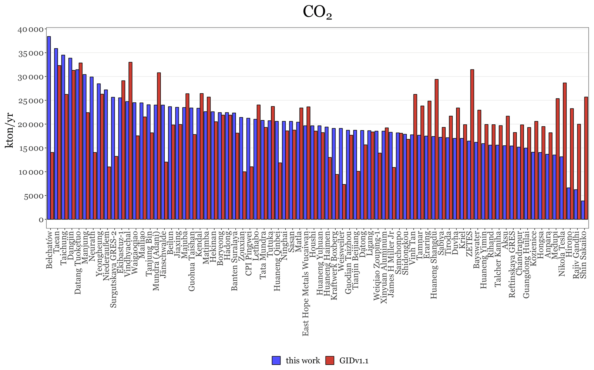
Figure 10 Comparison between plant-level CO₂ and the annual emissions (kt yr⁻¹) estimated by this work and reported by the GIDv1.1 database. Results are shown for the top 50 emitters of each inventory (a total of 76 facilities).

Additionally, we performed a plant-to-plant comparison between the top 100 CO₂ emitters reported by this work and the Central Electricity Authority (CEA, 2022) for India and the National Pollutant Release Inventory (NPRI, 2022) for Canada for the year 2018, finding overall good agreement between the datasets (R² between 0.79 and 0.81, Fig. S2).

3.2.2 Grid cell level

We added the CO₂ annual emissions of our point source catalogue to the same 0.1×0.1^∘ grid as the EDGARv7 CO₂ inventory and evaluated the spatial correlations between the two gridded datasets. Figure 11 shows the resulting spatial correlation obtained per country as well as comparisons of the CO₂ gridded distributions obtained with each dataset for the selected countries and regions. South Africa, Poland, Australia and the United States are the top 15 emitting countries, showing the largest spatial correlation and with values ranging between 0.77 and 0.88. Despite the high correlation obtained for South Africa, it is important to note that EDGARv7 does not report emissions in the grid cells where the Matimba and Medupi coal-fired stations are located. This discrepancy is relevant considering that the Matimba power plant is a typical case study in many top-down emission studies, as it is well isolated and easy to identify using satellite observations (e.g. Hakkarainen et al., 2021). Spatial correlations are in general larger in European and North American countries than in other regions such as Asia, the Middle East or Africa. This is in line with the fact that the spatial distribution of EDGAR emissions mostly relies on CARMAv3, which considers exact geographical coordinates for European, US and Canadian facilities but mainly city-centre latitude and longitude coordinates for the rest, as explained in Sect. 3.2.1. The reasons for the low correlations observed outside of these three countries and regions are many, including the aforementioned misallocation of CARMAv3 facilities, the non-inclusion of facilities that were built between 2009 (CARMAv3 reference year) and 2018 (reference year of the present work) or the inclusion of facilities that were retired in between these years and the inclusion of heat-only power plant emissions in EDGARv7, which are distributed according to population density. For instance, in Saudi Arabia the low correlation (0.05) is mainly linked to the different spatial patterns observed on the north-eastern coast, where this work presents a much larger number of grid cells with high emissions when compared to EDGARv7.

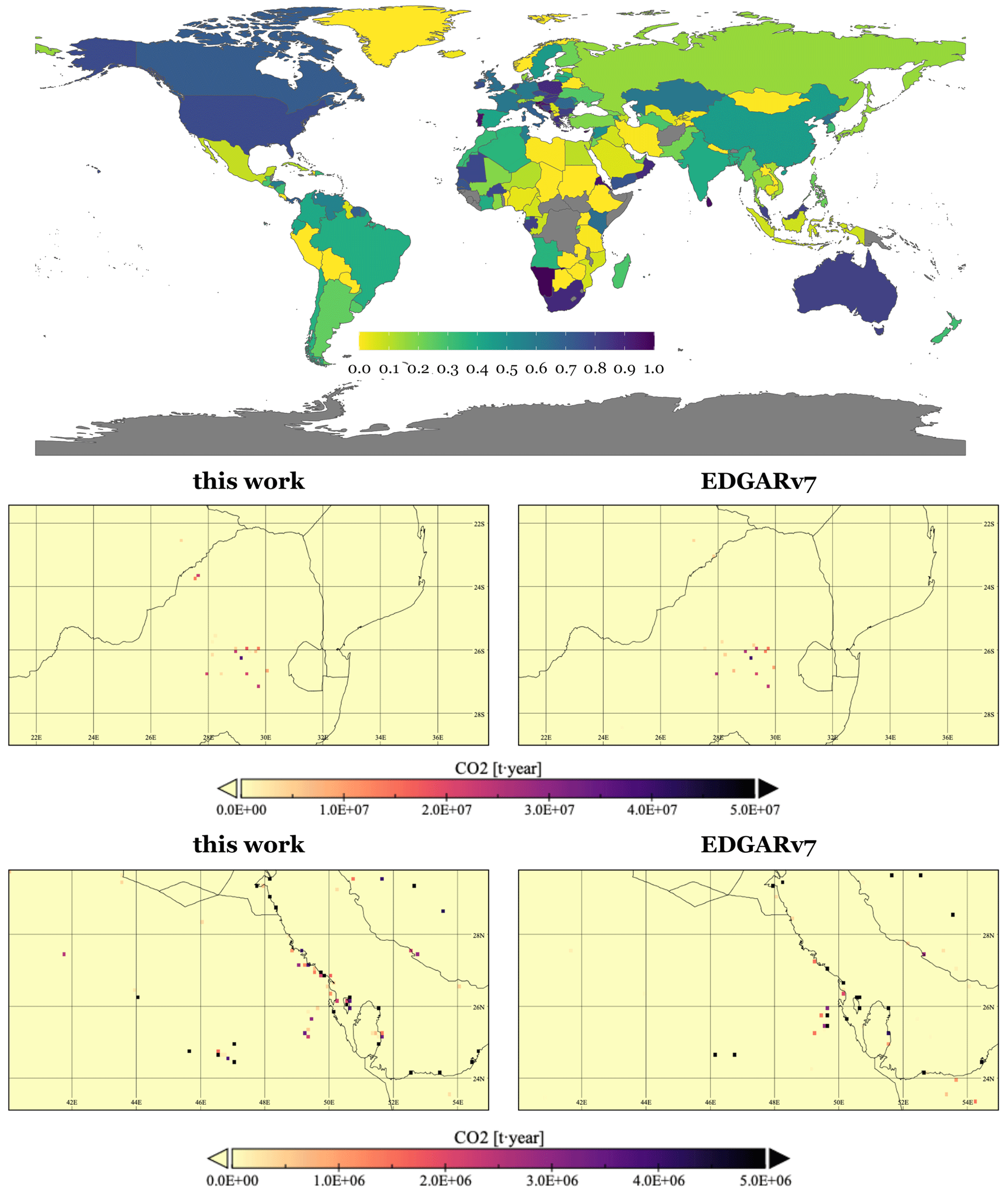
Figure 11 Map showing the spatial correlation between the power plant CO₂ emissions from this work and EDGARv7 at 0.1×0.1^∘ resolution per country. The maps below show a comparison between the 0.1×0.1^∘ gridded CO₂ annual emissions reported by this work and EDGARv7 in the northern region of South Africa and on the north-eastern coast of Saudi Arabia.

3.2.3 Country level

Estimated country-level emissions were compared against information reported by the EDGARv7 greenhouse gas (CO₂ and CH₄) and EDGARv6.1 air pollutant (NO_x and SO₂) global inventories as well as national estimates reported by the EMEP Centre on Emission Inventories and Projections (CEIP, 2022), the national inventory submissions to the UNFCCC (UNFCCC, 2022) and other national databases, including the USA National Emission Inventory (EPA, 2021), the Chinese Multi-resolution Emission Inventory model for Climate and air pollution research (MEICv1.3 for air pollutants and MEICv2.0 for CO₂; Li et al., 2017; Zheng et al., 2018), Cropper et al. (2021) and the GHG Platform India (2022) for India, the South African Atmospheric Emission License reports (AEL; ESKOM, 2022b), the Mexican National Emission Inventory (INEM; SEMARNAT, 2021), the Australian National Pollution Inventory (NPI; DCCEEW, 2022), the South Korean Clean Air Policy Support System (CAPSS; Choi et al., 2020) and the Taiwan Air Pollutant Discharge Inventory (TEDS; EPA Taiwan, 2021). For all the cases the reference year is 2018, except for the national estimates reported for the USA (2017), China (2017), Mexico (2016) and Taiwan (2019). Figure 12 shows the comparison for CO₂, CH₄, NO_x and SO₂ emissions in the top 20 emitting countries.

General good agreement is observed between the CO₂ emissions reported by this work and EDGARv7. The largest differences are observed in Russia, Japan and China, where the present catalogue reports lower emissions (−34 %, −15 % and −9 %, respectively) as it does not include auto-producers (Japan and India) and heat-only plants (Russia). The UNFCCC and independent national estimates are also generally in line with our work, the differences in China, the USA and India being 10 %, 9 % and −8 %, respectively. The discrepancies observed in the USA could be related to the fact that the national estimates reported by the UNFCCC do not include emissions from auto-producers (IPCC, 2019).

For CH₄, EDGARv7 tends to report larger emissions than this work, especially in Russia (−59 %), India (−52 %) and the USA (−29 %). In the case of Russia, national estimates are more aligned with EDGARv7 (21 %) than the present catalogue (−50 %). In contrast, in India and the USA, national emissions are more in line with estimates from this work than EDGARv7, the former presenting substantially higher values (32 % in the USA and 122 % in India). In Europe, the CH₄ emissions from this work sometimes match UNFCCC-reported values (e.g. Italy or Germany), but underestimations and overestimations also occur (e.g. Poland or the UK). Generally speaking, the share of the power sector in the total national CH₄ emissions is small, often around or below 1 % (e.g. 0.24 % for Italy, 0.19 % for Poland or 1.1 % for Sweden; UNFCCC, 2022). Hence, the deviations have a negligible influence on national total CH₄ emissions and are not further investigated. Moreover, CH₄ emissions in power plants are scarcely measured, and the corresponding emission factors are associated with very large uncertainties (IPCC, 2019).

EDGARv6.1 reports larger NO_x emissions than this work in all top 20 countries (by up to 3 times in Saudi Arabia). The emissions reported by our catalogue are more in line than EDGARv6.1 with the national estimates in most of the countries: China (differences of 26 % with this work and 46 % with EDGARv6.1), India (−26 % versus 49 %), the USA (16 % versus 222 %), Australia (−15 % versus 46 %) and Mexico (−15 % versus 108 %). Emissions reported by EDGARv6.1 in South Africa, Kazakhstan and Turkey are closer to the national values than our estimates, which are between 1.5 and 2.5 times lower. The discrepancies found for NO_x are much larger than the ones reported for CO₂. This is in line with the fact that the estimation of NO_x emissions is typically much more complex, as there are more elements that influence the emission rates, such as combustion conditions, combustion technologies or air pollution control levels implemented in the facilities. As described in Sect. 2.3.2, the ${\mathrm{NO}}_x/{\mathrm{CO}}_{\mathrm{2}}$ emission ratios considered in this work to estimate NO_x emissions in non-European countries are country-, region- and fuel-dependent, but they do not capture differences across power plants within the same country linked to e.g. different technological implementations.

For SO₂, comparison results are very similar to what is observed for NO_x. Emissions reported by this work are in general much lower than the EDGARv6.1 values (up to almost 4 times in the USA). When compared to national estimates, this study presents lower discrepancies than EDGARv6.1 in India, China, the USA, South Africa and Canada. In contrast, the comparisons performed for Turkey and Mexico indicate that EDGARv6.1 is closer to the national estimates, the present catalogue reporting 1.8 and 3.2 times lower values, respectively. Both EDGARv6.1 and this work present overestimations of similar magnitudes in Russia, Kazakhstan and Ukraine when compared to the independent national estimates (between 4.6 and 8.8 times). As mentioned for NO_x, we believe that the discrepancies observed between this work and national inventories are mainly related to the ${\mathrm{SO}}_{\mathrm{2}}/{\mathrm{CO}}_{\mathrm{2}}$ emission ratios considered, which cannot capture differences in emission abatement technologies or types of coals (e.g. sulfur content) used across facilities from individual countries.

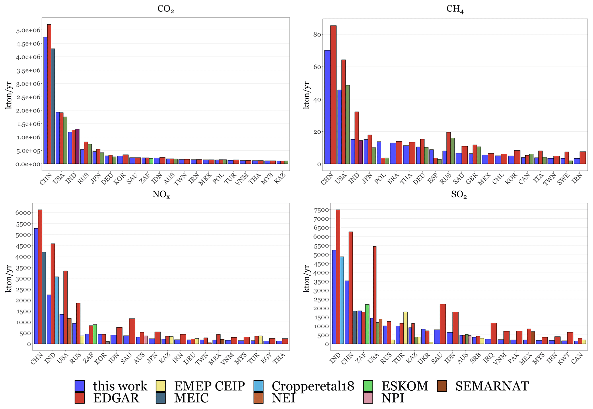
Figure 12 Comparison between country-level CO₂, CH₄, NO_x and SO₂ annual emissions (kt yr⁻¹) estimated for the power sector by this work and reported by independent inventories. Results are shown for the top 20 emitters.

Figure 13 shows the comparison of national CO₂ and NO_x emissions reported by the present catalogue and official estimates (UNFCCC and EMEP CEIP, respectively) for EU-27 + UK. Results from this work are distinguished between emissions directly obtained from the E-PRTR_v18 database and derived following the gap-filling routine described in Sect. 2.3.1.

For most countries there is good agreement with the nationally reported CO₂ total for the energy sector, which is not surprising since most countries will include the emission reporting by facilities in their national inventory. There are several countries, however, where the current catalogue sums to less than 60 % of the reported CO₂ national total: France, Denmark, Luxembourg, Austria, Lithuania, Latvia, Malta and Norway. When looking in more detail at the CO₂ emissions by fuel type (Fig. 14), the discrepancies for these countries appear to be caused by a significantly lower contribution of biomass CO₂ emissions. For example, for France, Austria and Denmark but also for Germany, the national inventory has much higher CO₂ emissions included from biomass combustion. The biomass or biogas power plants responsible for this contribution, however, mostly cannot be found in the EPRTR/LCP or other plant-specific databases that were consulted for this work (see Sect. 2.1). This suggests that these are mostly small-sized plants that fall below the reporting thresholds.

For NO_x, the differences are a bit larger than for CO₂, with the current catalogue covering on average about 88 % of the national total NO_x emissions. For Spain, the combined reporting of EPRTR facilities already substantially exceeds (by 73 %) the national reporting of energy sector emissions, which is related to the fact that national estimates reported to EMEP CEIP do not include emissions from the Canary Islands, as they are located outside the geographical scope of EMEP. As shown in Sect. 3.1, NO_x emissions from power plants located in the Canary Islands are substantial as they are operated by internal combustion diesel engines. For both CO₂ and NO_x, the influence of the gap filling of emissions appears limited on the national level.

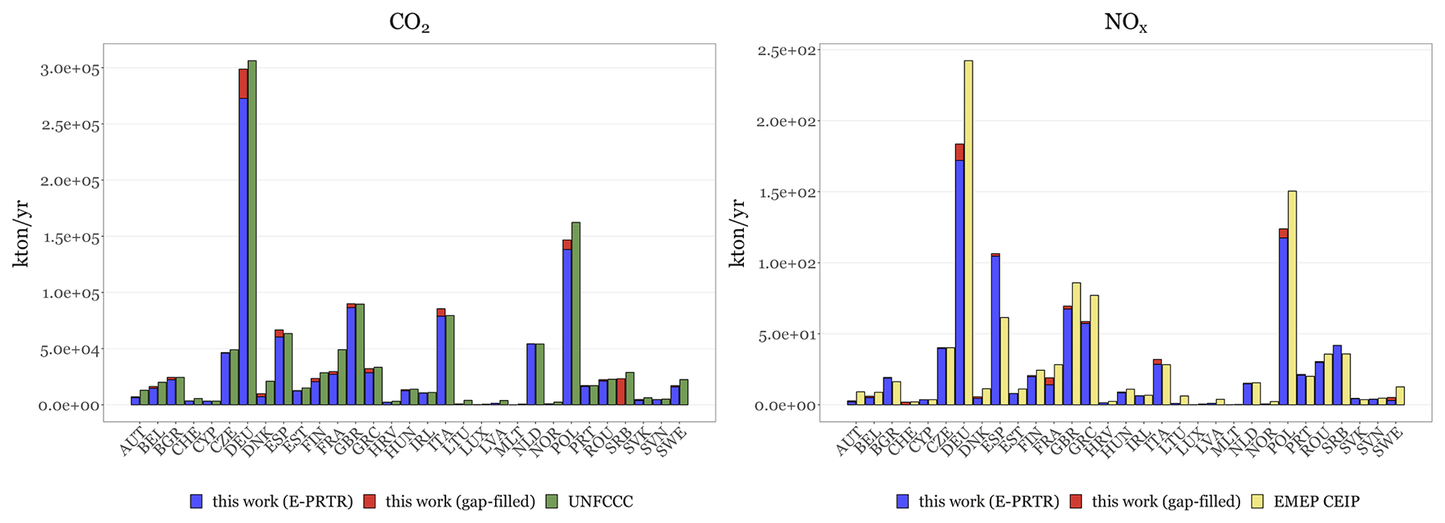
Figure 13 Comparison between country-level CO₂ and NO_x annual emissions (kt yr⁻¹) estimated for the power sector by this work and reported by EMEP CEIP and UNFCCC for EU-27 + UK. Results from this work are distinguished between emissions directly obtained from the E-PRTR_v18 database and derived following the gap-filling routine.

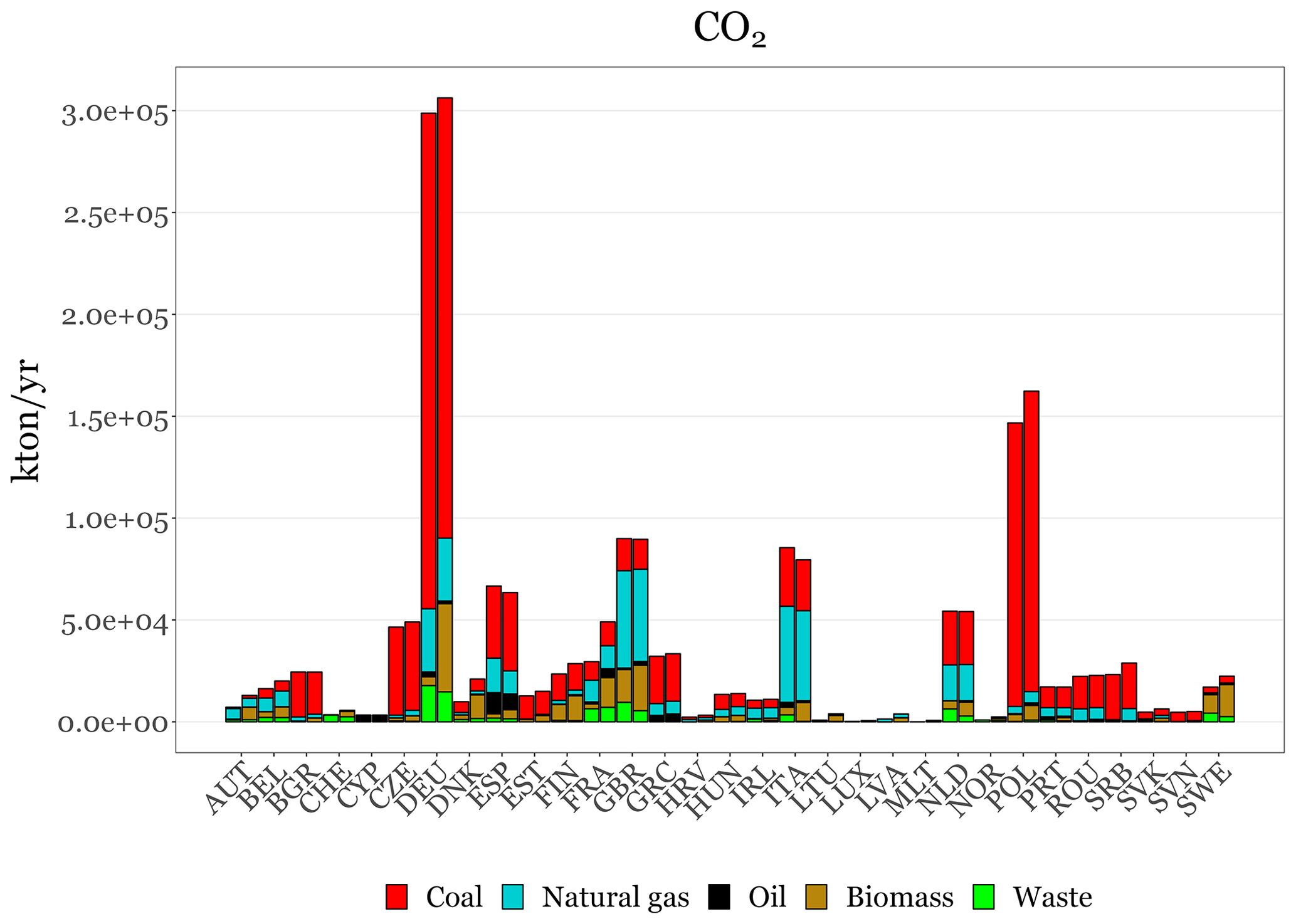
Figure 14 Comparison between country-level CO₂ annual emissions (kt yr⁻¹) estimated for the power sector by this work (left columns) and reported by UNFCCC (right columns) for EU-27 + UK by fuel type (coal, natural gas, oil, biomass, waste).

3.3 Temporal distribution

Figure 15 illustrates with an example the plant-level hourly CO₂ emission estimates (kg h⁻¹) obtained when combining the information on total annual emissions with the temporal profiles reported in the resulting catalogue. We used the HERMESv3 emission system (Guevara et al., 2020) to combine the total annual emissions per facility (Sect. 2.3) with the corresponding country- and fuel-dependent profiles (Sect. 2.4) and to derive hourly emissions for the year 2018. To distribute the annual emissions to hourly emissions per facility, the following relationship is used in HERMESv3 (Eq. 1).

$$\begin{array}{}\text{(3)}& E_{p,t}=E_p\cdot {\displaystyle \frac{M_{p,m}}{\mathrm{12}}}\cdot {\displaystyle \frac{W_{p,d}\cdot n_{d,m}}{\sum _{d=\mathrm{1}}^{\mathrm{7}}{W}_{p,d}\cdot n_{d,m}}}\cdot {\displaystyle \frac{H_{p,h}}{\mathrm{24}}}\end{array}$$

E_p,t are the hourly emissions (kg h⁻¹) for power plant p and date t (e.g. 27 November 2018, 17:00 UTC). E_p are the original annual emissions (kg h⁻¹) for power plant p. M_p,m is the monthly weight factor [0–12] for power plant p and month of the year m. W_p,d is the weekly weight factor [0–7] for power plant p and day of the week d [1 Monday–7 Sunday]. n_d,m is the number of day of the week d in month m, and H_p,h is the hourly weight factor [0–24] for power plant p and hour of the day h.

The results shown in Fig. 15 correspond to four coal-fired power plants: As Pontes (Spain), Belchatów (Poland), Jänschwalde (Germany) and Matimba (South Africa). The Matimba power plant is the facility that presents the flattest distribution, the results indicating that it is a base load power source. On the other hand, emissions from Belchatów, Jänschwalde and As Pontes present a clear seasonality, with emissions peaking during February, coinciding with a European cold spell that caused below-average temperatures in most European countries (C3S, 2018) and, in the case of As Pontes, also during summer, when energy demand increased due to the use of air conditioning systems. A weekend effect is also clearly observed for all the facilities, with emissions significantly dropping during Saturday and Sunday when compared to the weekdays.

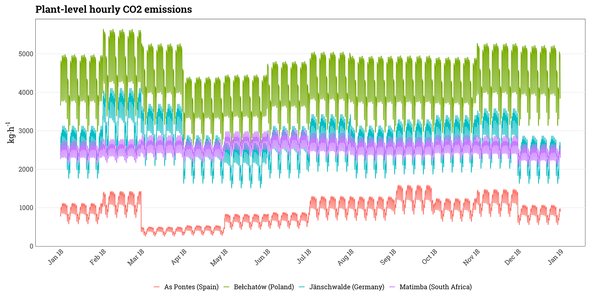
Figure 15 Estimated hourly CO₂ emissions (kg h⁻¹) for the As Pontes (Spain), Belchatów (Poland), Jänschwalde (Germany) and Matimba (South Africa) coal-fired power plants.

Country-dependent monthly, weekly and hourly profiles were constructed using as a basis the estimated plant-level hourly emissions. The resulting emissions were aggregated at the country level and were normalised to derive the corresponding temporal profiles. Results were compared against the temporal profiles reported by Denier van der Gon et al. (2011) for the power industry sector (hereinafter referred to as the TNO profiles), which are widely used in the modelling community to quantify observation-based emission estimates (e.g. Kuhlmann et al., 2021). Figure 16 shows examples of monthly, weekly and hourly profiles constructed for the power sector for selected countries and comparison against the TNO profiles.

At the monthly level, large variations are observed between countries. Profiles for the United Arab Emirates (ARE) and Kuwait (KWT) present a clear peak during summer, coinciding with the intensive use of air conditioning systems. In the case of USA Pennsylvania (USA-PA), we identify two types of peaks, one related to space cooling needs during July and August and another one linked to space heating needs during January and December. In Germany (DEU) and Poland (POL), we also distinguish the peaks during wintertime, while the increase in emissions during summer is much lower than the previous cases as these countries are at higher latitudes where summers are not too hot. The seasonalities in India (IND), China (CHN), South Africa (ZAF) and Australia (AUS) are much flatter. The TNO profiles were designed for Europe, and the mismatch for countries with different climatic regimes such as the United Arab Emirates and Kuwait is to be expected. Nevertheless, we can see that all the profiles differ significantly with the TNO profile, which reports a V-shaped seasonality, with emissions peaking during wintertime, presenting their lowest value during summer and therefore not capturing the peak related to space cooling needs, which is also relevant in Europe.

Concerning the weekly variability, profiles constructed for the European countries (i.e. Germany and Poland) are in line with the TNO profile, showing a strong weekend effect, with emissions being reduced by more than 20 % between weekdays and Sundays. On the other hand, profiles estimated for USA Pennsylvania, South Africa and Australia are much flatter (5 to 10 % differences between weekdays and weekends), while India shows almost no differences between weekdays and weekends.

Finally, constructed hourly profiles are quite consistent between countries, all of them showing a rather flat variation, with emissions being slightly larger (10 %–15 %) during daytime (between 07:00 and 20:00 LST). Similarly to what we see for the monthly profiles, large inconsistencies are observed between the constructed profiles and the TNO profiles, the latter showing a much larger variation between emission levels during nighttime and daytime and not reproducing the afternoon peak reported by the constructed profiles in most of the countries.

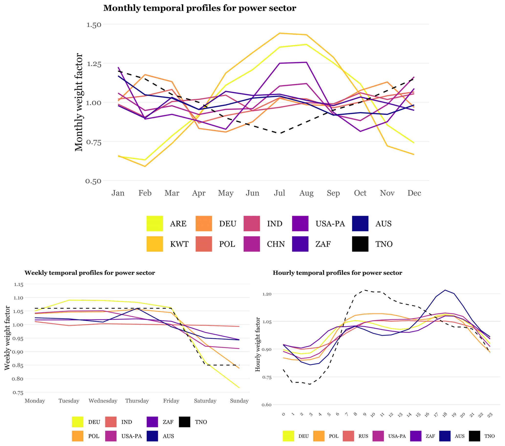
Figure 16 Power sector monthly, weekly and hourly profiles constructed for selected countries, including the Arab Emirates (ARE), Kuwait (KWT), Germany (DEU), Poland (POL), India (IND), China (CHN), USA Pennsylvania (USA-PA), South Africa (ZAF) and Australia (AUS). For each temporal resolution, estimated profiles are compared against the profiles reported by Denier van der Gon et al. (2011) (TNO).

The country-level monthly profiles derived in this work were also compared against the EDGAR temporal profiles (Crippa et al., 2020). We normalised the 2018 EDGARv7 CO₂ monthly emissions reported per country for the energy sector, which are calculated using the temporal distribution profiles described in Crippa et al. (2020) and then compared against our profiles. Figure 17 shows the correlation values obtained between monthly profiles per country as well as the comparisons between monthly profiles for selected countries. Correlations are large in several of the top 20 emitting countries (e.g. China, 0.75; Australia, 0.95; Russia, 0.92; Japan, 0.78; Mexico, 0.87; South Korea, 0.80; Taiwan, 0.89; Turkey, 0.95; Kazakhstan, 0.89). Low or even negative correlations are observed in some of the top emitters, including India ($r=-\mathrm{0.19}$), South Africa (r=0.16) and the United States (r=0.54). Nevertheless, when looking at the comparisons between monthly profiles reported in these three countries, we observe that both EDGARv7 and the present work suggest a very similar seasonality, with India and South Africa presenting a rather flat distribution and the United States showing two peaks in winter and summer, coinciding with the increase in electricity demand for space heating and cooling purposes, respectively. Brazil, Peru and Kuwait are among the countries presenting the largest negative correlation values (between −0.77 and −0.45). In the three cases, the seasonality reported by EDGARv7 and this work are completely opposite. While we suggest that emissions from the energy sector peak between June and September, coinciding with summer in Kuwait and southern winter in Brazil and Peru, EDGARv7 indicates that the largest emission levels occur between December and February (southern summer in Brazil and Peru). For these three countries, our profiles were constructed from national electricity generation statistics (see Table 5), while in the case of EDGARv7 they were indirectly estimated from regional averages computed using country-specific profiles belonging to the same world region. Most of the other countries for which a negative correlation exists are in Africa and Southeast Asia, where the information on electricity statistics to derive monthly profiles is rather scarce.

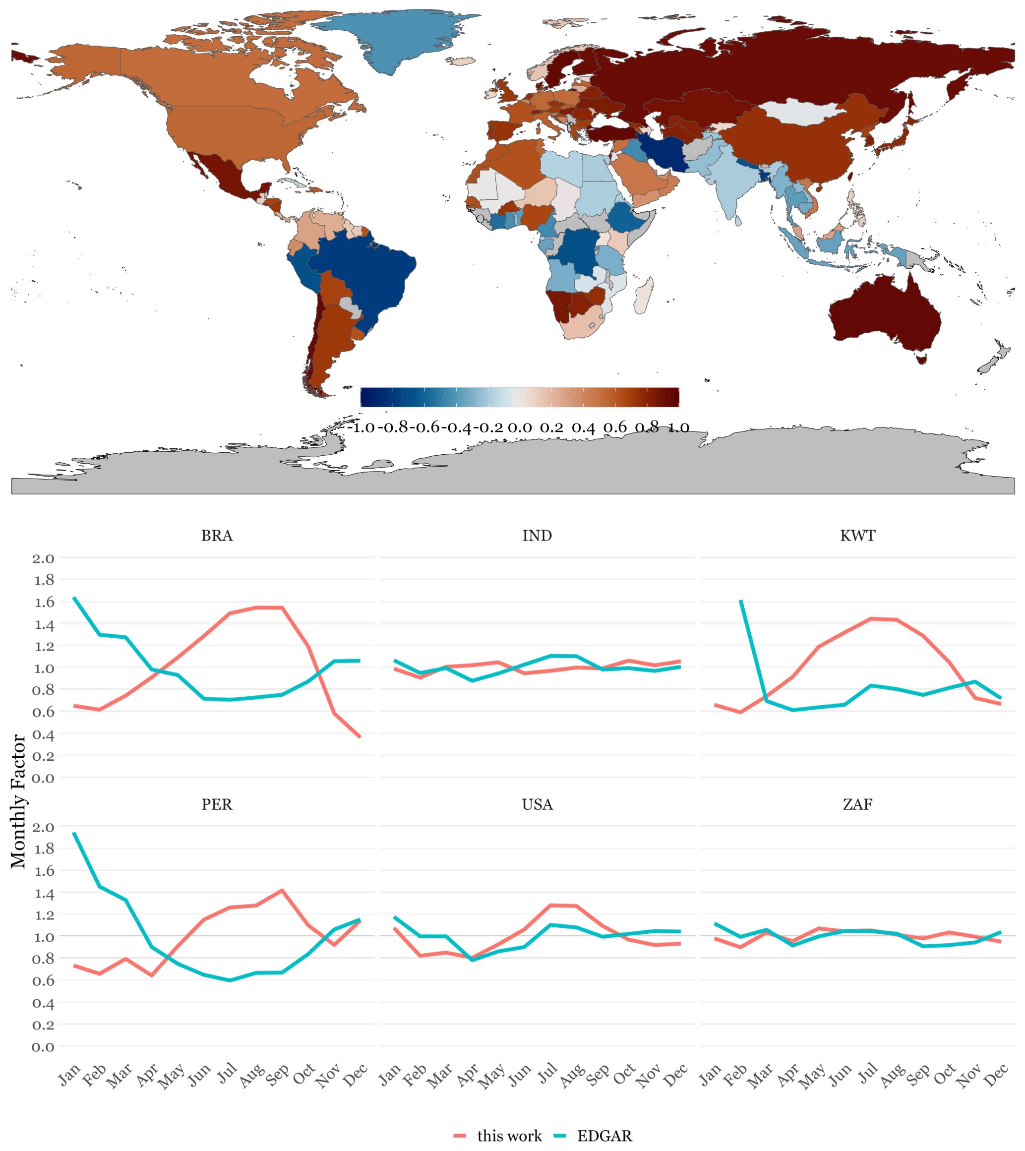
Figure 17 Map showing the correlation between monthly profiles constructed in this work and reported by Crippa et al. (2020) (EDGAR) for the energy sector per country. Countries in grey indicate that no correlation could be computed as no profiles are reported. The line plots below the map show the comparison between monthly profiles for selected countries.

The temporal profiles constructed in the present work are country- and fuel-dependent but are not facility-dependent. Large differences between the emission temporal distribution of plants belonging to the same country may occur, e.g. base load versus peak load, or if they are used for electricity only or electricity and heat. Figure 18 illustrates these differences by comparing the monthly, weekly and hourly profiles constructed in the present work for German coal-fired power plants (black solid lines) against profiles estimated for individual facilities making use of plant-level electricity generation statistics provided by ENTSO-E (2021). The comparison includes the top 20 producing coal-fired German power plants, which together supplied more than 75 % of the national electricity from burning coal in 2018. Profiles from power plants are represented with different colours and sizes that indicate their annual electricity production (the thicker and darker the line is, the more the electricity that is supplied). Results indicate a significant heterogeneity between profiles across plants. As expected, the more electricity a power plant produces, the more continuously it supplies electrical energy throughout the year and, subsequently, the flatter its associated monthly, weekly and hourly profiles are. By contrast, power plants producing less energy tend to show large variations between e.g. weekdays and weekends or between daytime and nighttime hours, as their behaviour is more linked to demand response. The discrepancies between our profiles and the plant-level profiles tend to be lower when looking at the top generating facilities. Consequently, our profiles better represent the temporal behaviour of those facilities emitting more emissions and that subsequently are easier to detect by satellite observations. However, important differences are still observed when comparing the profiles from the catalogue with the ones derived from the largest generating plant (i.e. Neurath), with differences of up to 18 %, 10 % and 8 % for the monthly, weekly and hourly weight factors, respectively. The largest discrepancies occur with the monthly distributions as they are influenced by many factors besides the typical changes in electricity consumption (e.g. more demand during weekdays than during weekends), including economic variables, meteorological conditions and electricity trade.

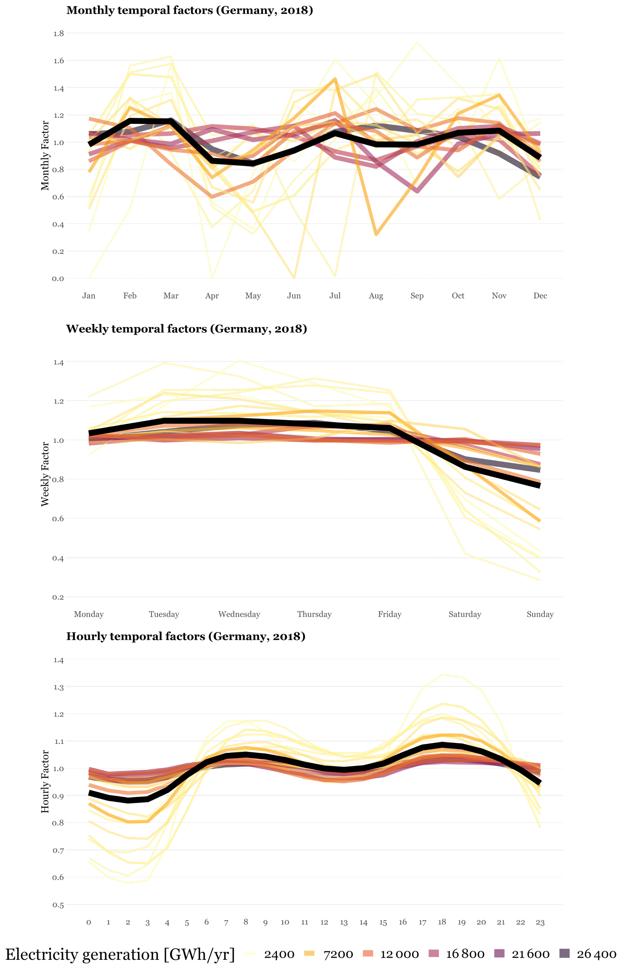
Figure 18 Comparison between monthly, weekly and hourly temporal profiles constructed in the present work for German coal-fired power plants (black solid lines) against profiles estimated for the top 20 producing coal-fired German facilities making use of plant-level electricity generation statistics (ENTSO-E, 2021). Profiles from power plants are represented with different colours and sizes that indicate their annual electricity production (GWh yr⁻¹).

3.4 Vertical allocation

Figure 19 shows an example of the daily bottom (blue) and top (red) plume values (m) at the Matimba (South Africa) and Bełchatów (Poland) coal-fired power plants estimated by the HERMESv3 model for the year 2018. Dashed lines indicate the stack height of each facility (i.e. 250 m for Matimba and 300 m for Bełchatów). Large month-to-month and day-to-day variations are observed for both the bottom and top plume heights at the two facilities, which are related to changes in the meteorological parameters and atmospheric stability driving the plume rise calculations, mainly the air temperature at the stack height and the boundary-layer height (Guevara et al., 2020). The bottom plume heights are, on average, 41 % (Bełchatów) and 70 % (Matimba) higher than the corresponding physical stack heights, while the top plume height values are on average 124 % (Bełchatów) and 206 % (Matimba) higher.

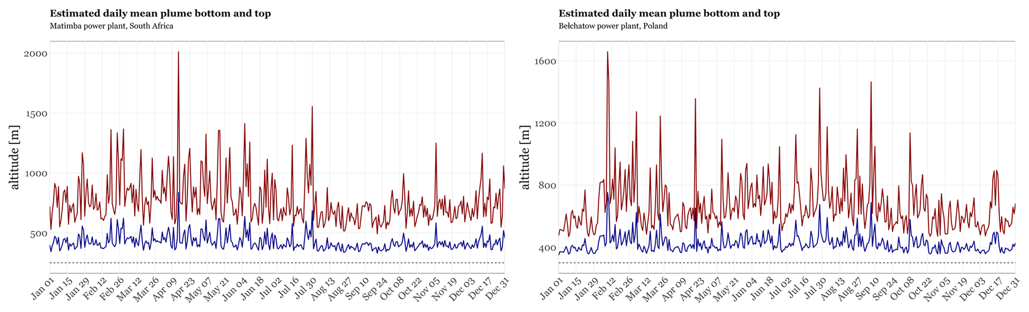
Figure 19 Estimated daily bottom (blue) and top (red) plume values (m) at the Matimba (South Africa) and Bełchatów (Poland) coal-fired power plants for the year 2018. Dashed grey lines indicate the stack height of each facility.

For each facility, the estimated CO₂ hourly emissions were first uniformly allocated across 16 vertical layers (from 0 m up to 1500 m with breaks every 100 m and above 1500 m) considering the modelled hourly plume top and bottom values, and they were then summarised to the annual level and finally normalised to 1 to derive annual and emission-weighted vertical profiles. Figure 20 shows the emission-weighted average annual vertical profiles computed for the As Pontes (Spain), Belchatów (Poland), Jänschwalde (Germany) and Matimba (South Africa) coal-fired power plants. The estimated profiles are compared against the vertical distribution proposed by TNO in the Copernicus CAMS-REG inventory for the public electricity and heat production sector (Kuenen et al., 2022). Jänschwalde is the power plant with the largest share of emissions occurring in lower layers (i.e. 78 % of the total emissions allocated between 100 and 300 m). This is due to the fact that emissions from this facility are released through the cooling towers, which have a height of only 120 m. On the other hand, As Pontes is the facility with the largest share of emissions allocated between 400 and 600 m (76 %), as it is the power plant with the highest chimney in Europe (365.5 m). Belchatów and Matimba present rather similar vertical distribution profiles, partially because both facilities have stacks of similar heights (300 and 250 m, respectively). Matimba is the power plant allocating the largest share of emissions across the top layers (8 % of total emissions above 1000 m). This is related to the larger exit velocity of the gases when compared to e.g. As Pontes (i.e. 26 versus 21 m s⁻¹, almost 25 % larger) and to differences in the local climatological conditions. The TNO profile distributes most of the emissions (85 %) between 200 and 500 m, the shares reported at higher altitudes (i.e. between 500 and 800 m) being considerably lower (8.5 %) than the ones computed for As Pontes, Belchatów and Matimba (between 32 % and 51 %). This discrepancy is in line with the fact that the TNO profile is derived from the work by Bieser et al. (2011), which assumed an average stack height of 159 m for calculating the plume rise in large power plants (>50 MW), a value significantly lower than the stack heights of the three power plants included in the comparison (365.5, 250 and 300 m). The results suggest that the TNO vertical profile may not be representative of power plants with high chimneys.

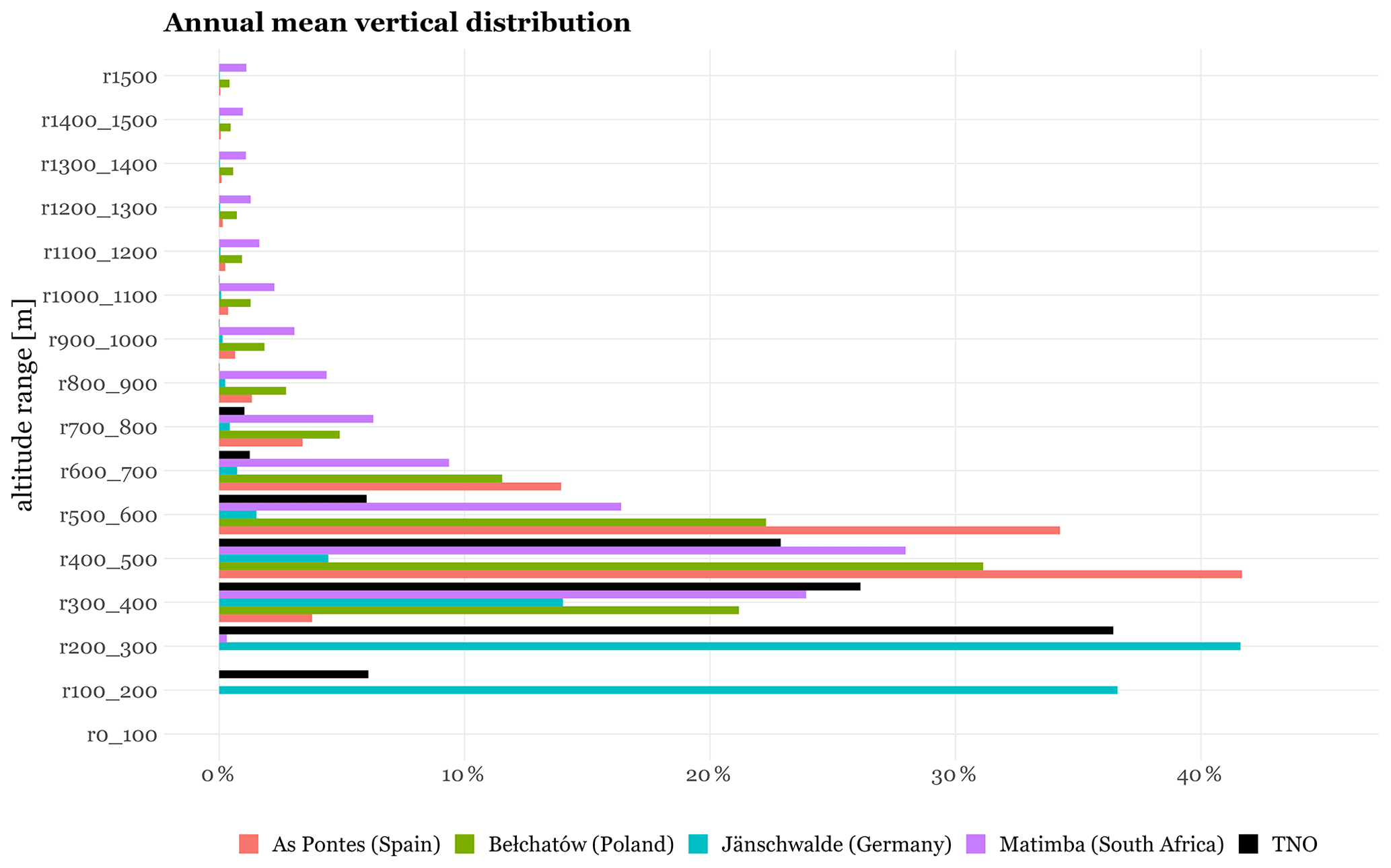
Figure 20 CO₂-emission-weighted average annual vertical profiles estimated for the As Pontes (Spain), Belchatów (Poland), Jänschwalde (Germany) and Matimba (South Africa) coal-fired power plants. For each facility we represent the associated vertical weight factors (%) across 16 vertical layers (from 0 m up to 1500 m with breaks every 100 m and above 1500 m). Estimated profiles are compared against the one provided by TNO in the Copernicus CAMS-REG inventory (Kuenen et al., 2022; TNO).

4 Data availability

The global catalogue of CO₂ emissions and co-emitted species from power plants, including plant-level total annual CO₂, NO_x, SO₂, CO and CH₄ emissions (t yr⁻¹), information on fuel type (i.e. coal, natural gas, oil, biomass and waste), geographical location (latitude and longitude coordinates in decimal degrees) and associated temporal profiles (monthly, weekly and hourly unitless weight factors that sum to 12, 7 and 24, respectively) and vertical profiles (normalised relative contributions of total emissions across 16 vertical layers from 0 m up to 1500 m, with breaks every 100 m and above 1500 m, which sum to 1), is provided in a collection of five CSV files through the CAMS document repository (https://doi.org/10.24380/0a9o-v7xe; Guevara et al., 2023). The CSV files included in the catalogue are the following.

• coco2_ps_catalogue_v2.0.csv: list of power plants with the associated total annual CO₂, NO_x, SO₂, CO and CH₄ emissions (t yr⁻¹); information on fuel type (i.e. coal, natural gas, oil, biomass and waste); geographical location (latitude and longitude coordinates in decimal degrees); and monthly, weekly and hourly temporal profile unique identifiers and vertical profile unique identifiers

• coco2_ps_monthly_profiles_v2.0.csv: list of monthly temporal profile unique identifiers with monthly weight factors (unitless) associated with each month (between 0 and 12)

• coco2_ps_weekly_profiles_v2.0.csv: list of weekly temporal profile unique identifiers with weekly weight factors (unitless) associated with each month (between 0 and 7)

• coco2_ps_hourly_profiles_v2.0.csv: list of hourly temporal profile unique identifiers with weekly weight factors (unitless) associated with each month (between 0 and 24)

• coco2_ps_vertical_profiles_v2.0.csv: list of vertical profile unique identifiers with the weight factor associated with each vertical layer (between 0 and 1). The distribution is defined across 16 vertical layers (from 0 m up to 1500 m with breaks every 100 m and above 1500 m).

The catalogue is provided together with a README file in .docx format that contains a description of each file of the global catalogue listed above and the associated fields of information. The catalogue is maintained as a GitLab repository hosted at https://earth.bsc.es/gitlab/mguevara/global_catalogue_power_plant_emissions/ (Guevara, 2023). Bug reports and other issues should be posted to the issue tracker at https://earth.bsc.es/gitlab/mguevara/global_catalogue_power_plant_emissions/-/issues (Guevara, 2023). The catalogue is licensed under Creative Commons Attribution 4.0 International (CC-BY-4.0: https://creativecommons.org/licenses/by/4.0, last access: August 2023).

5 Limitations of the dataset

The current catalogue provides an updated and high-resolution global picture of the spatial (horizontal and vertical) and temporal characterisation of emissions from power plants. Despite all the efforts, there are, however, some limitations associated with the current version of the dataset that potential users should consider.

• Emissions from non-European auto-producer facilities are not consistently included across countries due to the lack of information. Overall, we could not include emissions from auto-producers in 35 % of the non-EU countries considered, which translates to 4.1 % of the total estimated CO₂ emissions that could not be allocated to specific point sources. The most relevant countries affected by this limitation are Russia, India and Japan, and the share of national emissions that could not be assigned to individual facilities for these countries is between 14 % and 21 %.

• For the non-European dataset, heat-only facilities are not included due to the lack of information. This gap may be relevant in countries where the share of fossil fuels used to produce heat only is significant, mainly Ukraine (25 %), Russia (20 %), Belarus (20 %), Kyrgyzstan (18 %) and Uzbekistan (10 %).

• We identified a list of countries for which we found the locations of their power plants but which we could not include in the final catalogue since their energy balances are not reported by the IEA World Energy Balances database, and subsequently, the corresponding emissions could not be estimated. It is important to note that most of these missing countries are small island countries (e.g. Aruba, Anguilla, American Samoa Antigua and Barbuda, Bahamas, Fiji, Cabo Verde or the Cayman Islands), which have a very limited contribution to the total CO₂ emissions from the power sector (i.e. 0.03 % according to Tong et al., 2018).

• For the European dataset, a substantial number of emission values was gap-filled using a tiered routine and using facility-specific or more generic pollutant ratios to estimate emissions. In total, gap-filled emission values contribute less than 10 % to the total emissions for CO₂, NO_x and SO₂ but more than 60 % for CO and CH₄. In terms of emission values for individual locations, close to 50 % of the power plants have been gap-filled for CO₂ and NO_x, 80 % for SO₂ and above 90 % for CO and CH₄. These results indicate that gap filling plays a more prominent role in small- and medium-sized combustion facilities and that emission values from large power plants are typically reported. The approach implemented could however lead to underestimations or overestimations of emissions for individual plants, especially for NO_x and SO₂ and the important role of air pollution control levels in this species, which can vary across facilities.

• The non-European coal-, natural-gas- and oil-fired power plant emissions from co-emitted species (NO_x, SO₂, CO) were estimated using fuel-, country- or region-dependent emission ratios derived from the GAINS inventory that reflect national emission standard aspects. However, pollution abatement controls differ not only by country or region, but also across power plants within the same country. The use of not only fuel- and country-dependent but also technology-dependent emission ratios could potentially help in reducing this uncertainty.

• For the non-European dataset, plant-level emissions were estimated by distributing fuel-dependent national emissions among facilities as a function of their installed capacity, which in some cases may not be representative of their actual activity (i.e. capacity factor) and may lead to overestimations or underestimations.

• For the European dataset, there was mostly good agreement with the national inventory totals for the energy sector in the case of CO₂ and NO_x. The main source of discrepancies appeared to be the missing biomass power plant capacity in the dataset. These plants are likely too small to be included in official reporting and most public power plant datasets, e.g. because they fall below reporting thresholds. A more in-depth look into these biomass plants is needed to improve coverage and completeness.

• The final catalogue of power plants covers the main fuels used to produce energy and heat, including coal, natural gas, oil, solid biomass and solid waste. However, we are still missing some fuels that are relevant in specific countries and for emissions from certain species (e.g. CH₄) such as biogas (e.g. Thailand, India, Turkey or Australia) and liquid biofuel (e.g. South Korea).

• The comparison between geographical locations reported by the present catalogue and the CARMAv3 database indicates that the locations of the current top emitters are better represented in this work, especially in Asian countries such as China, Taiwan and India, where the majority of the CARMAv3 facilities are assigned city-centre latitude and longitude coordinates. Despite putting substantial efforts into correcting the locations of facilities that were originally reported with wrong coordinates, there may still be some error present in the dataset, especially in the cases of small- and medium-sized plants.

• Concerning the representativeness and stability of the temporal profiles constructed for 2018 over the years, we refer to the analysis performed by Crippa et al. (2020) in which monthly temporal profiles for the power generation sector for the 35 Organisation for Economic Co-operation and Development (OECD) countries over the time period 2000–2017 were analysed. According to their results, large standard deviations mainly occur in countries where the use of fossil fuels to generate electricity is rare, such as Finland, Iceland, Norway or Sweden, where more than 90 % of the total electricity comes from renewable sources or where the number of fossil fuel power plants that supply energy to the grid is very low (e.g. Latvia, with five natural gas power plants). These situations can cause large relative year-to-year changes in the monthly profiles, as they are more sensitive to changes in meteorological conditions or the dynamics of specific facilities, among others. On the other hand, the year-to-year variations of the monthly profiles obtained for the top emitting countries (e.g. China, Japan, the USA or Australia) are in general much lower.

• The temporal profiles assigned to the power plants are country- and fuel-dependent, but they are not facility-dependent. Large differences between the emission temporal distribution of plants belonging to the same country may occur, e.g. base load versus peak load power plants or electricity and heat versus heat-only power plants. A comparison between the monthly, weekly and hourly profiles constructed in the present work for German coal-fired power plants (black solid lines) against profiles estimated for individual facilities supports this hypothesis but also indicates that our profiles are sufficiently capable of representing the temporal behaviour of the top emitting facilities, which are easily detected by satellites. However, important differences are still observed when comparing the profiles from the catalogue with the ones derived from the larger generating plants, especially at the monthly scale, for which an important heterogeneity between the plants exists due to the influence of changes not only in the demand but also in the meteorological conditions, economic variables and electricity trade. The development of plant-level profiles is nevertheless limited by the lag of information on plant-level electricity generation statistics, which is currently limited only to certain regions (e.g. EU-27).

• The final database provides plant-level annual mean vertical profiles that consider meteorology and stack parameter information. However, large variations in the vertical distribution of the emissions may occur between seasons, days of the year and hours of the day due to changes in the meteorological parameters that influence the atmospheric stability and the corresponding vertical dispersion of the emissions.

• Despite identifying several power plants in which emissions are released through the cooling towers instead of the traditional chimneys (mainly in Germany), there may still be multiple facilities in the catalogue that are not correctly flagged. Moreover, for power plants using the cooling towers to release the emissions, we considered the same plume rise formulas as the ones used for traditional stack chimneys. According to Brunner et al. (2019), this assumption may entail an underestimation of the resulting effective emission height of 20 % to 100 % due to the combination of several factors, including the additional release of latent heat from cooling towers or the interaction of plumes from cooling towers located next to each other.

• The stack parameter information used to perform the plume rise calculations has a limited coverage (e.g. only 28 % of the total CO₂ emissions have specific stack height information and only 15 % specific exit velocity data), which may bring additional uncertainty to the estimated vertical profiles. According to the sensitivity runs performed by Bieser et al. (2011), changes in estimated emission heights are almost linear with changes in stack height and exit velocity, indicating a large influence of these parameters on the result.

• Caution should be used when combining the global point source dataset with other existing gridded emission inventories (e.g. EDGAR) to avoid issues of double counting or incompleteness. Avoiding these problems can be challenging if, for instance, the sector classification of the gridded inventory is broad (e.g. emissions from power plants are included together with emissions from refineries and other energy industries in the same sector). A reclassification of the gridded emissions may be needed in these cases to ensure an appropriate combination of datasets.

6 Conclusions

We present a high-resolution catalogue of CO₂ emissions and co-emitted species (NO_x, SO₂, CO, CH₄) from thermal power plants for the year 2018. The construction of the database follows a bottom-up approach, which combines plant-specific information with national energy consumption statistics and fuel-dependent emission factors and emission ratios. Annual emissions are provided for each plant at its exact geographical location. Each facility is linked to a country- and fuel-dependent temporal profile (i.e. monthly, day of the week and hourly) and a plant-specific vertical distribution profile, which allows us to derive spatially and temporally resolved emissions for modelling purposes. The resulting catalogue has been developed in the framework of the Prototype System for a Copernicus CO₂ service (CoCO2) EU-funded project to support the development of the CO2MVS capacity. Results from the catalogue were compared to widely used and state-of-the-art emission inventories like the Carbon Monitoring for Action (CARMA), the Global Infrastructure emission Database (GID) and the Emissions Database for Global Atmospheric Research (EDGAR), as well as officially reported emission data.

6.1 Future perspective

The current point source catalogue represents an effort to improve the spatial (horizontal and vertical) and temporal characterisation of emissions from CO₂ and co-emitted species derived from power plants to be used for modelling efforts. Future work should focus on overcoming the limitations currently identified (see Sect. 5) and extending the temporal coverage to more recent years in order to capture, on the one hand, the impact of the decarbonisation efforts that are occurring in several countries and regions such as EU-27, the UK or the USA and, on the other hand, the large uptick in commissioning of new coal power plants that is happening in China (https://www.carbonbrief.org/mapped-worlds-coal-power-plants/, last access: January 2024). In parallel, other large CO₂-emitting industries that are detected by satellite instruments, including cement and steel-and-iron plants, should be added in future versions of the global point source database.

The current catalogue does not report prediction intervals or standard errors of the estimated emissions for each plant. Hence, the uncertainty information is unknown. The comparison against independent inventories indicates good agreement for CO₂ but also important discrepancies for NO_x and SO_x, highlighting that the co-emitted species estimates and their uncertainty deserve more attention in future research. This is in line with the fact that the estimation of NO_x and SO_x emissions is typically much more complex than for CO₂, as there are more elements that influence the emission rates, such as combustion conditions, combustion technologies or air pollution control levels implemented in the facilities. Including information on the emission abatement technologies implemented in each plant could help define more detailed (i.e. technology-level) emission ratios for the estimation of co-emitted species. Unfortunately, none of the other plant-level emission inventories used for comparison includes information on co-emitted species, and therefore plant-level emission comparisons were limited to CO₂. In this sense, performing intercomparisons against existing satellite-derived point source catalogues (e.g. Beirle et al., 2023; Fioletov et al., 2023) could also help to better constrain bottom-up emissions from co-emitted species.

The present work revealed that information on stack parameters is currently limited not only in developing countries but also in developed regions such as EU-27. Efforts should be made to compile this information from individual national environmental permits and to centralise it in a European database, at least for the large point sources considered under the European Industrial Emissions Directive (2010/75/EU). Furthermore, flagging of the power plants with channel emissions through cooling towers should be assessed to better represent the vertical distribution of these emissions.

Finally, future works will include performing study applications that show the impact of using this emission catalogue on modelling results.