the Creative Commons Attribution 4.0 License.
the Creative Commons Attribution 4.0 License.
 | 17 Jul 2024
Multitemporal characterization of a proglacial system: a multidisciplinary approach
Elisabetta Corte
Andrea Ajmar
Carlo Camporeale
Alberto Cina
Velio Coviello
Fabio Giulio Tonolo
Alberto Godio
Myrta Maria Macelloni
Stefania Tamea
Andrea Vergnano
The recession of Alpine glaciers causes an increase in the extent of proglacial areas and leads to changes in the water discharge and sediment balance (morphodynamics and sediment transport). Although the processes occurring in proglacial areas are relevant not only from a scientific point of view but also for the purpose of climate change adaptation, there is a lack of work on the continuous monitoring and multitemporal characterization of these areas. This study offers a multidisciplinary approach that merges the contributions of different scientific disciplines, such as hydrology, geophysics, geomatics, and water engineering, to characterize the Rutor Glacier and its proglacial area. Since 2020, we have surveyed the glacier and its proglacial area using both uncrewed and crewed aerial surveys (https://doi.org/10.5281/zenodo.8089499, Corte et al., 2023c; https://doi.org/10.5281/zenodo.10100968, Corte et al., 2023f; https://doi.org/10.5281/zenodo.10074530, Corte et al., 2023g; https://doi.org/10.5281/zenodo.10101236, Corte et al., 2023h; https://doi.org/10.5281/zenodo.7713146, Corte et al., 2023b). We have determined the bathymetry of the most downstream proglacial lake and the thickness of the sediments deposited on its bottom (https://doi.org/10.5281/zenodo.7682072, Corte et al., 2023a). The water depth at four different locations within the hydrographic network of the proglacial area (https://doi.org/10.5281/zenodo.7697100, Corte et al., 2023d) and the bedload at the glacier snout (https://doi.org/10.5281/zenodo.7708800, Corte et al., 2023e) have also been continuously monitored. The synergy of our approach enables the characterization, monitoring, and understanding of a set of complex and interconnected processes occurring in a proglacial area.
- Article
(14349 KB) - Full-text XML
-
Supplement
(5989 KB) - BibTeX
- EndNote


In memory of Velio Coviello.
Global warming is entailing a rapid decline in the cryosphere globally. Mountain snow cover and glaciers respond directly and rapidly to climate change, making them key indicators of global warming. The intensity and frequency of precipitation are changing, and part of the precipitation has shifted from solid to liquid due to the increased temperatures (e.g., in the European mountains). This shift and the increasing number of dry and warm winter days in the European Alps are reducing snow accumulation. In addition, the rising air temperature in spring is increasing snowmelt, modifying the local water balance (Carrer et al., 2023; Gizzi et al., 2022). Snowfall and ice melt/snowmelt impact glacier mass balance. As a consequence of global warming, glaciers within the European Alps are subject to a reduction in surface area and ice mass (Sommer et al., 2020).
Most glaciers reached their Holocene maximum extent at the end of the Little Ice Age (LIA), a cooler period in the Holocene lasting from the 1300s to the 1850s (Ivy-Ochs et al., 2009), and have receded since then (Grove, 2004). The decline in snow cover and glaciers exposes more land and water surfaces to solar energy, leading to decreasing albedo and to weathering, resulting in increased erosion. Glaciers produce a considerable amount of sediment (Hallet et al., 1996), the size of which ranges from large boulders to fine sands, silt, and clay (Hallet et al., 1996; Carrivick and Tweed, 2021). Depending on dynamic and thermodynamic conditions, glaciers have the ability to entrain sediment and erode bedrock. Even when the entrainment capacity is reduced, glaciers retain the ability to deform the sediment (Alley et al., 1997).
Using the terminology defined by Slaymaker (2011), the area encompassing the glacier outline at the end of the LIA and the present-day glacier terminus is the proglacial area. Proglacial areas are considered systems in transition from glacial to non-glacial conditions; therefore, they are natural laboratories that allow the investigation of the early stages of newly exposed soil development, vegetation succession, and associated soil stability and sediment fluxes (Matthews, 2019). Due to global warming and glacial retreat, disequilibrium occurs between sediment delivery from the glacier and fluvial reworking in proglacial areas (Slaymaker, 2011). Their evolution depends on the interaction between geomorphic processes and vegetation succession. On the one hand, plant colonization stabilizes glacial sediment and reduces sediment fluxes; on the other hand, geomorphic processes disturb and limit vegetation succession (Curry et al., 2006; Moreau et al., 2008; Eichel, 2019).
Studies investigating multiple processes within a proglacial area at scales larger than a single landform or a hillslope and at different timescales are not frequent (Hilger and Beylich, 2019). The integration of all of the processes involved in the sediment budget requires a catchment-wide identification, mapping, and quantification of all relevant sediment transport processes; a localization and monitoring of the storage elements in the sediment transport system; and a localization of their interaction areas (Hilger and Beylich, 2019). Carrivick and Tweed (2021) state that the remobilization of sediment within the proglacial area mainly determines the sediment yield in a proglacial area. Guillon et al. (2018), in their study of the Bossons Glacier (France), found that sediment sources vary according to season: sediment remobilization within the sandur is the dominant source of sediment in autumn, whereas the main export of sediment comes from the glacial source during the melt season. Further efforts to integrate multiparametric observations and enhance interdisciplinary scientific collaboration are needed to predict sediment dynamics in a warming world (Zhang et al., 2022)
Sediment availability is strongly governed by morphology (Cavalli et al., 2018). The land-system elements of a proglacial area have different geomorphic functions and are heterogeneously distributed. These elements can act like sediment sources, stores (short-term storage landforms), and sinks (long-term storage landforms) (Matthews, 2019). In Alpine catchments, runoff depends on rainfall events, snow, and glacier melt (Camporese et al., 2014). Glacier retreat in response to the local climate is heterogeneous in space and time and so is the water regime. Sediment yield depends on runoff and sediment availability, which are both highly variable in space and time (Heckmann and Schwanghart, 2013; Hooke, 2000; Carrivick and Tweed, 2021). Furthermore, the connection among water discharge, bedload, and suspended sediment transport exhibits variability over the years and within seasons, influenced by climatic conditions, as highlighted in previous studies (Mao et al., 2018; Coviello et al., 2022).
In this work, to the best of our knowledge, we present the first public dataset of a proglacial area that is the result of hydrological, geophysical, geomatics, and water engineering monitoring. This dataset is the result of a multidisciplinary approach and represents the input data to assess the water and sediment balance in the Rutor proglacial area and the morphodynamics occurring in recently exposed soils. The synergy among different disciplines has allowed for a holistic viewpoint in the observation of the evolutive phenomena of the Rutor proglacial area to be achieved.
2.1 Site description
Rutor Glacier lies at the head of the Dora Baltea Valley in La Thuile, near the France–Italy border in northwestern Italy. It is mainly oriented to the northwest and exists at an altitude ranging from 2540 to 3486 m a.s.l. (meters above sea level), with an average altitude close to the average value for Alpine glaciers, as retrieved from the Global Land Ice Measurements from Space (GLIMS) database (GLIMS Consortium, 2005; Raup et al., 2007). Rutor Glacier is among the glaciers with the largest surface area in the Alps, and it is the third largest glacier in the Aosta Valley (GLIMS Consortium, 2005; Raup et al., 2007). At present, it has a surface area of 7.5 km2, and its front is formed by three tongues (Fig. 1) that were once united (Fig. 2). Villa et al. (2007) determined the Rutor Glacier retreat and volume changes from the mid-19th century to 2004. Since 2005, the regional environmental protection agency of the Aosta Valley (ARPA-Valle d'Aosta) has been monitoring the mass balance of Rutor Glacier, which (with the exception of the years 2013, 2014, and 2016) has always been negative, resulting in a cumulative mass balance from 2005 to 2017 of −12 252 mm w.e. (millimeters water equivalent) (ARPA Valle d'Aosta, 2014). Since its maximum extent in the LIA (Orombelli, 2005; Villa et al., 2007), the glacier has lost approximately 34 % of its surface area. The retreat and lowering of the glacier surface are not uniform: these changes are more pronounced in the eastern tongue (Villa et al., 2007).
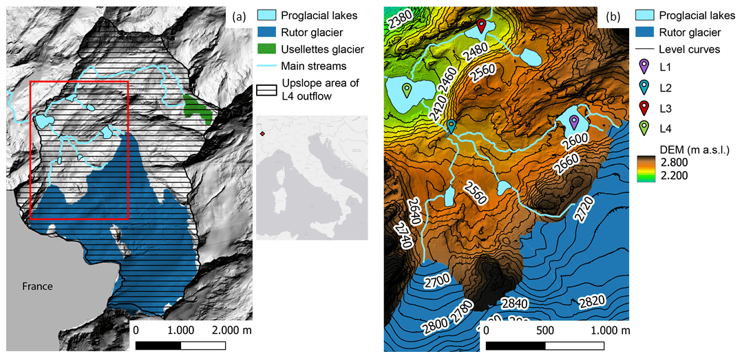
Figure 1(a) Hillshade based on the digital surface model (DSM) of Rutor Glacier and the L4 lake catchment as of 2008. The upslope area of the L4 outflow (hatched area with continuous black lines) has been mapped using the 2008 model of Aosta Valley (SCT Geoportale, Regione autonoma Valle d'Aosta, 2024). The inset shows the study location in Italy. (b) DSM of the Rutor proglacial area and locations of the L1, L2, L3, and L4 proglacial lakes as of 2021.
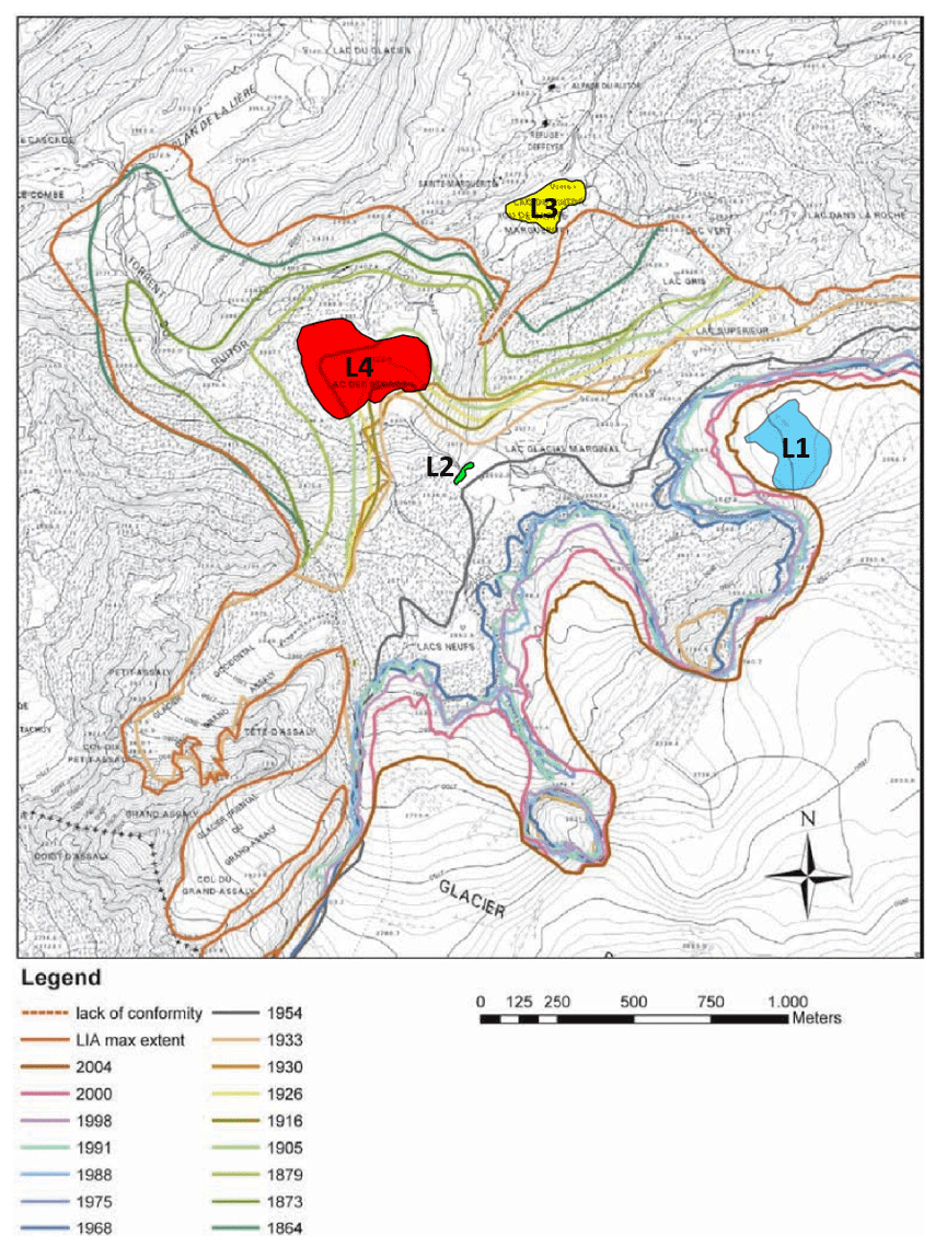
Figure 2Reconstruction of the Rutor Glacier terminus from its maximum extent in the LIA to 2004 (modified from Villa et al., 2007). The areas highlighted in blue, green, yellow, and red indicate the current extent of lakes L1, L2, L3, and L4, respectively.
The entire Rutor proglacial area spans approximately 4 km2 (Villa et al., 2007). This area holds significant importance for the investigation of sediment dynamics in proglacial systems, owing to its geomorphological diversity and pristine condition, resulting from minimal human impact. Notably, the presence of L4, which acts as a basin closure within the proglacial area, collects all mobilized sediment within the region. Since the end of the LIA, Rutor Glacier has retreated, leading to a progressive increase in the proglacial area. The glacier recession has exposed topographic depressions which determined changes in stream networks and the formation of several proglacial lakes. These lakes act as sediment sinks, interrupting sediment transfer from the glacier outlet to the lowlands. The altitude from the lowest proglacial lake to the glacier terminus (middle-tongue snout) ranges from about 2390 to 2660 m a.s.l. The land-system elements within the Rutor proglacial area include steep slopes, outwash plains (sandurs), and single and braided channels, while the alluvial channel beds and banks vary in size from fine sands, silt, and clays to boulders. L1 has a single outflow which, after a distance of 830 m, flows into a sandur. This sandur is fed by the meltwater of the entire glacier and has a surface area of about 0.1 km2. Due to a topographic barrier, the water is forced to flow downstream from the outwash plain through a single channel. When the water level in the sandur rises, the abovementioned topographic barrier determines the formation of the L2 lake (2504 m a.s.l.). The water flows from the L2 to the L4 proglacial lake (Lake Seracchi, 2387 m a.s.l.) via a steep creek with an elevation jump of about 100 m.
The outflows of L2 and L3 (Santa Margherita Lake) are the only two surface inflows of the L4 lake, whose outflow feeds the majestic Rutor waterfalls. The L4 lake collects all meltwater from Rutor Glacier and is the major and most downstream proglacial lake of the analyzed area. Its outflow cross-section is quite stable and allows one to easily measure the lake outflow. As the main processes involving the water and sediment budget of the Rutor proglacial area occur upstream and within L4, the study focuses on the basin area upstream of the outflow control section of L4; this specific study region has an overall catchment area of 18.12 km2, 43 % of which is glacierized (see Fig. 1a).
The characteristics of the study area described above can be easily observed via a web geographic information system (WebGIS) available at https://arcg.is/Tyeju0 (last access: 15 February 2024).
Among all of the lakes in the area, the Santa Margherita Lake – here named L3 (2422 m a.s.l.) – has been the most thoroughly monitored in the past because of catastrophic outburst floods (Baretti, 1880; Sacco, 1917); these floods began in the first half of the 15th century, showing that the glacier had already retreated at that time (Sacco, 1917).
The past evolution of the L3 lake serves as evidence of the changes that the whole area had gone through due to the glacier retreat since the end of the LIA. These changes have been reported in several documents (e.g., Sacco, 1917; Baretti, 1880; Valbusa and Peretti, 1937), allowing for the reconstruction of the changes in the glacier and its proglacial area.
2.2 Multidisciplinary framework
Assessment of the water balance and sediment budget implies the identification of the different physical processes involved, their geomorphic function, their contribution to the overall sediment production, and their effectiveness in supplying sediment to the main stream (Hilger and Beylich, 2019). Quantifying the sediment budget of proglacial areas is a challenging task due to the multitude of processes involved as well as their spatial and temporal variability. Most studies either (1) focus on a single landform or hillslope at different times (e.g., Laute and Beylich, 2014; Curry et al., 2006) or (2) measure river-basin-scale production rates at the outlet of the basin (e.g., Hicks et al., 1990; Müller, 1999; Bogen et al., 2015). The following paragraph provides a concise overview of the monitoring methods used in three distinct studies concerning different proglacial areas.
Guillon et al. (2018) combined sedimentary measurements with precipitation data to understand present-day suspended sediment storage and erosion processes during a melt season. They measured water depth and turbidity, deriving the respective water discharge and suspended sediment concentration at three different stations. Orwin and Smart (2004) characterized a proglacial channel over a 9-week ablation period by continuously measuring the water depth and turbidity at different gauging stations distributed within the proglacial area. Confirming that sediment yield varies both spatially and temporally within a proglacial area, Delaney et al. (2018) assessed erosion rates and processes in an Alpine proglacial area using digital surface models (DSMs), reservoir bathymetry, and a glacial–hydrological model (GERM). Water discharge measurements were determined by the water level at the reservoir located at the basin outlet. The first two reported studies (Guillon et al., 2018; Orwin and Smart, 2004) provided an explanation for the spatiotemporal variation in proglacial suspended sediment flux, but they did not assess the landscape evolution of the geomorphological features in the whole proglacial area; in contrast, in the latter reported study (Delaney et al., 2018), the sediment processes in the whole proglacial area were identified, but the water discharge was directly measured only at the basin outlet. The abovementioned studies hold important value with respect to understanding the dynamics in proglacial areas, but there is a lack of work in the literature involving repeated surveys (e.g., photogrammetric flights) and continuous monitoring (e.g., flow measurements) at several points in the proglacial and glacial area.
Table 1Timetable of continuous measurements and field surveys; the first column shows the measured quantities/surveys, while the bottom row presents the timeline. The colors and symbols are characteristic of the respective measuring stations and surveyed areas (see legend). The arrows between the dates indicate that the measurements are continuous between the dates.
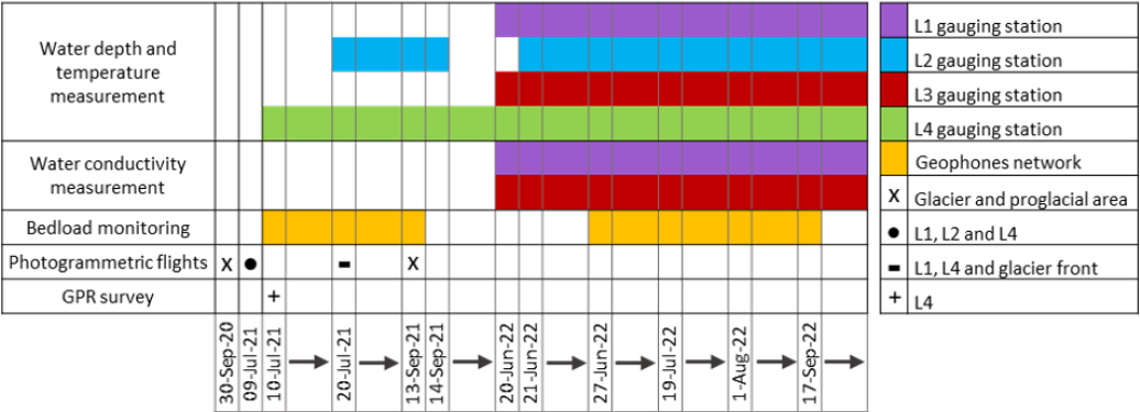
As of 2005, the local environmental agency of Aosta Valley (ARPA-Valle d'Aosta) has been monitoring the mass balance of Rutor Glacier via direct in situ measurements. Since 2020, the Glacier Lab of the Polytechnic University of Turin has integrated ARPA surveys with geophysical and geomatics measurements. In the summer of 2021, the area monitored by the Glacier Lab increased from 25.2 to 34.5 km2 to include the proglacial area.
Our monitoring activities at Rutor Glacier can be categorized into multitemporal and continuous surveys. An overview of these monitoring activities is provided in Table 1.
2.3 Geomatic survey: aerial acquisitions and Global Navigation Satellite System (GNSS) positioning
Rutor Glacier was monitored with different geomatics techniques, supported by different surveying campaigns, with the following two aims: (i) to provide a common 3D reference system to properly manage all of the spatial and temporal datasets of the different research groups involved in the glacier monitoring and (ii) to enable the 4D (3D over time) monitoring of the extent and morphology of the glacier surface. The geomatics surveys started in 2020 and include both uncrewed and crewed aerial photogrammetric flights as well as topographic measurements in the field. The geomatics surveys were carried out in parallel with the activities of the other Glacier Lab teams in order to acquire in situ data and enable the implementation of integrated multidisciplinary monitoring activities.
In the 2020–2021 period, the surveys described in Table 2 were carried out. Among those, during the summer campaigns in 2021, three photogrammetric flights (one on 9 July 2021 and two on 20 July 2021) were carried out using a DJI Phantom 4 RTK uncrewed aerial vehicle (UAV) multirotor platform (using the UAV's built-in camera equipped with a 1 in, 25.4 mm, RGB sensor) to survey the proglacial lakes.
Table 2Photogrammetric flights carried out on the study area between 2020 and 2021.
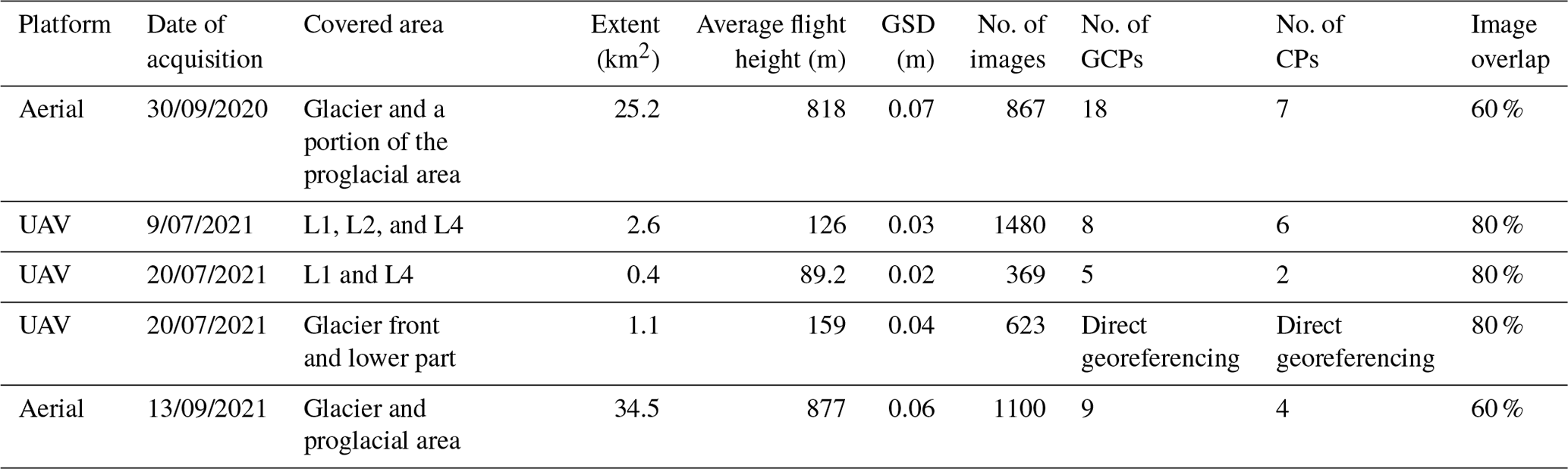
After the summer of 2021, at the end of the 2020–2021 hydrological year, crewed photogrammetric flights were carried out by the Digisky company over the glacier and proglacial area, using a medium-format PhaseOne camera iXM-RS150F installed aboard an ultralight aircraft. The crewed aerial flight was carried out with a P90e light aircraft; its handling allows easy flight altitude changes to maintain a constant ground sampling distance (GSD). The camera has a focal length of 50 mm, a sensor size of 40 mm × 53.5 mm and a resolution of 151.3 MP. The 2021 photogrammetric survey was a repetition of a previous flight that had been carried out at the end of September 2020 with the same aerial platform and sensors but a smaller coverage (without complete coverage of the L2, L3, and L4 lakes).
The datasets acquired during the UAV and aerial photogrammetric flights were processed to obtain a 3D model of the terrain and additional cartographic products, i.e., orthophotos and DSMs. A standard structure-from-motion (SfM) photogrammetric approach was adopted, following a consolidated workflow using the Agisoft Metashape software. This approach progressed as follows:
-
image alignment, to estimate interior/exterior (relative) orientation parameters, generating a relative sparse point cloud using feature detection and matching and SfM-based bundle block adjustment with self-calibration;
-
collimation of ground control points (GCPs; not relevant in the case of a direct georeferencing approach) to re-estimate interior/exterior (absolute) orientation parameters (refining the previous step), generating a georeferenced sparse point cloud;
-
evaluation of residuals on GCPs and check points (CPs) and iteration of the previous step in the case of anomalies in the residuals;
-
generation of a dense point cloud;
-
generation of a digital surface model (with respect to a cartographic plane) and orthoimagery.
The photogrammetric processing reports generated by the Metashape software for the two crewed aerial flights (the only ones used for elevation analyses) are available in the Supplement (https://doi.org/10.5281/zenodo.11144390, Corte et al., 2024). These reports include information on processing parameter settings, survey data details, camera calibration, camera locations, GCPs, and CPs.
During the 2021 field activities, a total of 32 artificial photogrammetric markers, either square (0.5 m × 0.5 m) plaster markers or crosses painted on stable rocks, were positioned (or painted) and measured with a real-time kinematic (RTK) and static Global Navigation Satellite System (GNSS) positioning approach, using three Spectra Precision SP80 GNSS receivers (static data have been processed with RTKLIB software). The markers were distributed on the proglacial area (to ensure stability over time), around L4, and along L1 until the glacier front on the eastern tongue. Among the 32 markers, 12 larger markers (1 m × 1 m) were positioned around the top part of the glacier area during the September 2021 campaign in order to enable straightforward identification on aerial images. The markers placed in 2021 were used as both GCPs and independent CPs (details in Table 2) for the 2021 crewed aerial survey. Considering that the focus is on relative displacements rather than on absolute values, 25 natural GCPs and CPs were then identified on the 2021 orthomosaic and DSM to orient the 2020 crewed aerial imagery and assess its 3D positional accuracy (considering that the artificial markers were not yet available in 2020). A GCP- or CP-based approach has also been used for UAV surveys (two markers used for the aerial dataset were also leveraged for the UAV datasets), except for one UAV survey in which, exploiting the RTK capabilities of the UAV GNSS receiver, a direct georeferencing approach was adopted (considering it was not possible to place markers in the glacier front area for safety reasons). Direct georeferencing refers to the orientation of remotely sensed imagery without using GCPs, exploiting real-time kinematic (RTK) or post-processing kinematic (PPK) approaches. An RTK- or PPK-based approach enables the generation of metric products with 3D positional precision and accuracy in the range of few centimeters (Chiabrando et al., 2019; Teppati Losè et al., 2020a, b).
As the camera positions of aerial flights were not geotagged with proper accuracy, it was necessary to exploit the artificial markers to georeference the 3D model accurately over the entire glacier area. The cartographic reference system adopted for all of the 3D models is ETRF2000/UTM32N; the ellipsoidal height was reduced to orthometric height by applying the Italian geoid model ITALGEO05. Due to the availability of a suitable number of well-distributed GCPs, the 2021 aerial survey was considered to be the reference model (referred to as “Model Zero”) to be used for multitemporal analyses. The 2020 survey was, therefore, co-registered (i.e., georeferenced in the same reference system, enabling the overlap of all of the derivative products) with the 2021 survey.
As one of the main objectives is the evaluation of relative displacements between multitemporal 3D models and the main focus is on the elevation component, multitemporal DSMs were compared using a pixel-by-pixel approach. It has to be highlighted that, as the focus is on the entire glacier area and UAV flights cover only the terminus of one of the glacier tongues, the elevation analysis described in this paper is related solely to the crewed aerial dataset. In particular, the aerial DSM 2020 was subtracted from the aerial DSM 2021 to calculate the altimetric differences, referred to as the difference of DSM (DoD). The following section is focused on the assessment of the positional accuracy of the datasets derived by the aerial photogrammetric flights, specifically on the elevation.
DSM validation: DoD and limit of detection (LoD) estimation
To properly assess the photogrammetric results (i.e., in this specific case, the DSMs and their differences), it is necessary to apply “suitable statistics to identify systematic error (bias) and to estimate precision” and to propagate “uncertainty estimates into the final data products” (James et al., 2019). When comparing DSMs from two different epochs (t0 and t1), their DoD values need to be evaluated with reference to the limit of detection (LoD), i.e., the threshold for the significance of the DoD values.
The estimation of the LoD, with a certain level of significance, can be conducted either (i) by analyzing altimetric residuals at specific independent CPs or (ii) through the analysis of areas that remain unchanged over time, where significant altimetric variations are not expected (i.e., stable terrain) (Paul et al., 2017). Each method has its own advantages and disadvantages. For this particular multidisciplinary study, it has been decided to determine the LoD based on the analysis of residuals at CPs. This decision was made both to adopt a cautious approach (the relative LoD value at 95 % is slightly less favorable compared with that derived from stable areas) and because it was not feasible to identify uniformly distributed stable areas across the entire region covered by the photogrammetric surveys.
The first approach relies on the statistical analysis of altimetric residuals (ΔZ) at some independent CPs, which are points with known coordinates that, unlike GCPs, have not been used during the photogrammetric image orientation parameter estimation phase. Preliminarily, it is important to highlight the difficulty in acquiring independent CPs with field measurements in glacial areas and, generally, in high-mountain zones, due to both the limited presence of suitable areas for establishing points and the intrinsic difficulties and related constraints with respect to movements. Despite having a limited sample of CPs, it is possible to perform a statistical analysis to assess the altimetric accuracy and precision of DSMs, particularly by calculating the mean (to analyze possible systematic errors) and standard deviation of ΔZ, respectively. Naturally, these statistics are also calculated for the planimetric residuals ΔX and ΔY, as significant planimetric systematic errors would also influence altimetric precision. The results of such analysis can be summarized in a table structured similarly to Table 3.
Table 3Means and standard deviations of the residuals ΔX, ΔY, and ΔZ calculated on GCPs and CPs.

ΔK is the residual of K for each CP, μΔK is the mean of ΔK values calculated for all CPs, σΔK is the standard deviation of ΔK values calculated for all CPs, and K is a generic component (X, Y, or Z) of the 3D coordinates of each CP.
Mean values significantly lower than the standard deviation imply, in the case of ΔZ residual analysis (where a distribution with a mean of zero is expected), the absence of systematic errors, which – if present – should be corrected before proceeding with the estimation of the LoD. The LoD – at a 95 % confidence level – of the differences between two multitemporal DSMs (acquired at epochs t0 and t1) can thus be derived from the variance propagation law applied to σΔZ (last column of Table 3), as demonstrated in Brasington et al. (2000) and Lane et al. (2003). In particular, under the assumption of normal distribution and independence of variables:
In this context, t1 and t0 designate the specific temporal points considered for the multitemporal analysis, indicating the respective acquisition dates of the source data utilized to produce the DSMs.
Alternatively, or in support of, the analysis based on CPs, the estimation of the LoD can be conducted using differences in DSMs over time, derived from multitemporal analysis on areas of the terrain considered “stable” over time. These stable areas must be meticulously delineated outside of glacial regions susceptible to melting or, more generally, subject to changes. Except for potential outliers, the values of DoD should tend towards zero in stable terrain (considering the stability of the areas and the altimetric precision of the DSMs). For determining the LoD of the DoD, even with the approach based on stable areas, it is necessary to statistically analyze the altimetric differences. In particular, the distribution of DoD values, unlike the CP-based approach, will involve a large number of points (even millions of points), significantly increasing statistical significance. Preliminarily, however, it is necessary to remove any outliers to evaluate whether the distribution of DoD follows a normal distribution with a mean of zero (given that the DoD concerns stable terrain) and to estimate its variance. Outliers may arise from either localized terrain variations not identified during the delineation of stable areas or potential errors in the automatic correlation of the photogrammetric process in regions with “monotone” texture. The process of excluding outliers can be carried out by removing the tails of the DoD distribution, for example, by eliminating the top and bottom 5 % of the distribution tails. Once the normality of the distribution is confirmed, it is possible to compute the mean and standard deviation of the DoD (σDoD) on the sample without the top and bottom 5 % of the distribution tails. In analogy to the CP-based approach, the LoD can be then calculated as 2 times the σDoD (see Eq. 7).
2.4 Geophysical survey
The bathymetry of Lake Seracchi and the thickness of the sediments deposited on its bottom were determined using a ground-penetrating radar (GPR) (Sambuelli et al., 2015) supported by time domain reflectometry (TDR) measurements (He et al., 2021), as reported in more detail in Vergnano et al. (2023).
Both systems are based on the principle of the propagation of high-frequency electromagnetic signals, in the bandwidth between 30 MHz and 1 GHz. The signal propagation in natural media depends on the electromagnetic properties of the media (dielectric permittivity and electrical conductivity). In a low-conductivity material, the signal propagates with a velocity related to the dielectric permittivity, according to , where c is the electromagnetic wave velocity in vacuum and ε is the relative dielectric permittivity of the material (Psarras, 2018). The velocity is usually estimated in the time domain: a signal pulse is excited by an antenna (in GPR) or TDR device and propagates into the medium; part of the energy carried out by the signal is scattered back (or reflected) when a contrast in electromagnetic impedance is encountered. The amount of energy that is reflected depends on the contrast in electrical conductivity or dielectric permittivity between two different media. The backscattered signal is then collected by an antenna (receiving antenna in GPR) or by an oscilloscope (in the case of TDR devices). In the GPR, the amplitude of the signal that is backscattered at the interface between two different media defines the reflectivity of the target. The GPR approach for detecting the bathymetry of a lake is based on the reflectivity of the lake bottom, based on the contrast in dielectric permittivity between water and sediments of the lake bottom.
The dielectric permittivity of water depends on the temperature, and it is slightly affected by salinity; typical values at low temperatures are around 80 (relative values, referring to the dielectric permittivity of vacuum), corresponding to an electromagnetic (e.m.) wave velocity in water of around 0.033 m ns−1. In our case, with a 6 °C temperature and a relative permittivity of 83.3, the wave velocity was estimated to be 0.0327 m ns−1. High-porosity sediments could exhibit dielectric permittivity in the range between 35 and 40. This means that the water–sediment interface should exhibit good reflectivity, given the contrast in dielectric permittivity values.
The GPR antenna, manufactured by IDS GeoRadar s.r.l., had a central frequency of 200 MHz, which provides the best possible resolution while avoiding the energy dispersion that occurs in water at frequencies higher than 200 MHz (Bradford et al., 2007). The GPR system was installed on an inflatable rowing boat, and the boat was moved to cover the whole area of the lake. The GPR sections acquired were processed according to a set of standard processing steps, performed in Reflexw software (Sandmeier, 2021; Vergnano et al., 2023) and reported in Appendix C.
The x–y–z locations of the first interface, representing the lake bottom, detected in all of the GPR sections were interpolated with a linear triangulation-based method (griddata function of MATLAB) to produce a bathymetry map (Fig. 11, which also displays the sediment thickness distribution and the electrical conductivity measurements). The perimeter of the lake, retrieved from the 6 cm resolution orthophoto acquired on the day of the geophysical survey, was useful to fix the zero depth in the interpolation process.
The TDR probe, installed on a rod, was inserted in the lake bottom sediments at several locations and measured their electrical conductivity and dielectric permittivity. The valence of the TDR survey is twofold:
-
First, it can be used to corroborate the interpretation of the GPR sections, as the point values of dielectric permittivity give an estimation of the electromagnetic wave velocity in the sediment (v), necessary to convert the GPR travel times into thickness of the sediments itself. Also, the dielectric permittivity can be used to define the expected reflectivity of the water–sediment interface and to estimate the sediment porosity, as the sediment is considered to be fully saturated.
-
Second, it can be utilized to assess the spatial variability in the type of sediments by measuring their electrical conductivity. In fact, the electrical conductivity of the lake sediments depends on the porosity, water salinity and temperature, and texture of the sediments; the electrical conductivity is a good indicator of the presence of finer material, as the bulk electrical conductivity usually increases due to the contribution of the surface electrical conduction of the finer particles.
To validate the GPR and TDR measurements, geotechnical analyses (grain size distribution and Atterberg limits) were performed on a few sediment samples collected at the locations shown in Fig. 11 (see Vergnano et al., 2023, for more details).
2.5 Hydraulic monitoring
The hydrography of the Rutor proglacial area is made complex by a sequence of flat and steep areas, by the presence of several proglacial lakes that are connected differently, and by the contribution from three tongues of the glacier. In order to assess the partial and total surface runoff, four instruments were installed to measure the water depth at different locations in the study area. The location of these water pressure gauges was determined by the accessibility and the geometry of the channel or lake and the presence of stable rocks or banks on which to install the instruments.
Two types of instruments were installed: (i) a self-contained water logger and transmitter measuring water level and temperature (OTT ecoLog 1000) and (ii) a combined measurement of water level, temperature, and conductivity (OTT CTD). The four locations of the gauges stations, from upstream to downstream, are the L1 emissary, L2, the L3 emissary, and the outflow of L4 (Fig. 3). Water depth allows one to retrieve (from direct velocity measurements) the water discharge, while conductivity measurements allow water characterization for surface or groundwater flow, which is a matter of interest for L3 and L4. Therefore, the two OTT CTD instruments were installed in the L1 and L3 emissaries. The ecoLog1000 and CTD instruments were first installed in July 2021 and June 2022, respectively; the measuring periods of each sensor are shown in Table 1.
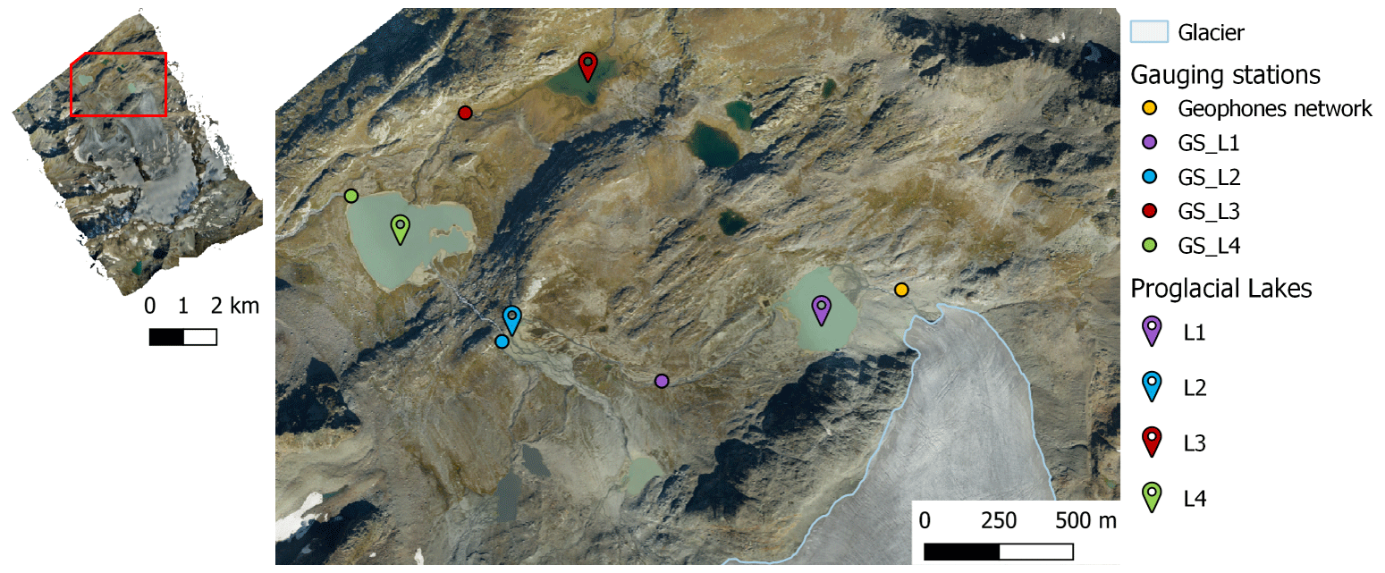
Figure 3Aerial orthophoto of the Rutor proglacial area acquired on 13 September 2021 and the snout of the Rutor eastern tongue. The red polygon in the upper left orthophoto shows the position of the area enlarged in the right orthophoto. The lakes (L1, L2, L3, and L4), the gauging stations, and the geophone network are indicated.
The upslope areas of the four sensors installed are as follows: 5.3 km2 for the L1 gauging station, 12.6 km2 for the L2 gauging station, 4.9 km2 for the L3 gauging station, and 18 km2 for the L4 gauging station.
As the area covered by the photogrammetric flights (2020 and 2021) excluded a portion of the upstream area of the L1 and L3 gauging stations, these areas were determined using the 2008 DSM of Aosta Valley (SCT Geoportale, Regione autonoma Valle d'Aosta, 2024).
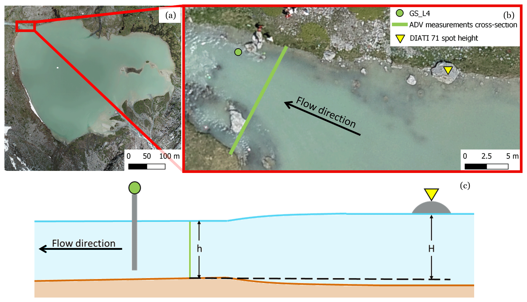
Figure 4(a) Orthophoto of L4 (July 2021). (b) Close-up of the L4 outflow where the ADV measurements were taken; the DIATI 71 spot height is also shown. (c) A longitudinal cross-section of the L4 outfall showing the reference water depth of the emissary (h) and the reference total head measured in the lake (H).
At all of the cross-sections of the gauging stations, with the exception of L2, the flow velocity was measured with a current meter. At L2, due to the high flow velocity during the summer season, direct measurements are not safe for the operator. To derive the discharge from the water level measurements, a stage–discharge (or rating) curve has to be developed. In the summer of 2021 and 2022, a set of nine flow velocity measurements were taken with an acoustic Doppler velocimeter (ADV) current meter in the cross-section of gauging station L4. The velocity-based discharge measurements (Q) were related to the corresponding water depth (h) measured at the gauge (Fig. 4), to plot the stage–discharge diagram (Fig. 5a; further details on the procedure are given in Appendix A).
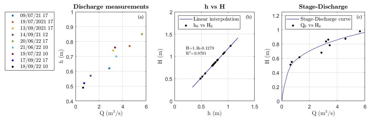
Figure 5(a) Discharge measurements (Q) in the L4 emissary and the corresponding water depth (h). (b) Measurements of the total head (H) and the corresponding water depth (h). The linear interpolation equation and the coefficient of determination (R2) are reported. (c) Discharge measurements (Q) and the corresponding total head (H) as well as the stage–discharge curve for the L4 emissary.
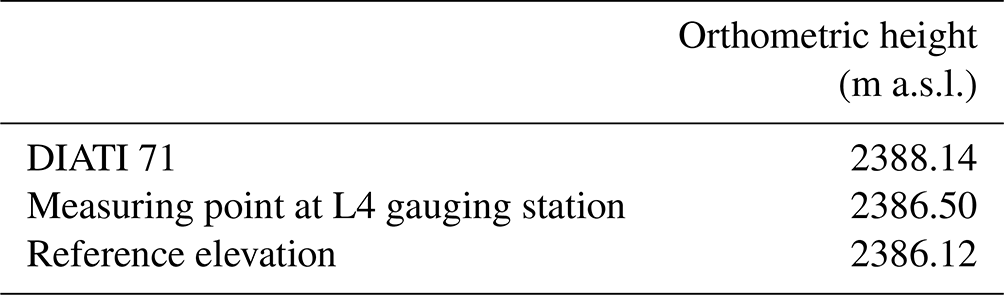
L4 is the largest and most downstream lake of the area collecting the meltwater of Rutor Glacier and the suspended sediment of the upstream area. Monitoring the water level and the outflow of L4 is crucial to assess the water and sediment budget of the Rutor proglacial area. Due to backwater effects at the outflow, the water levels in the lake and the control cross-section are not identical, but they are strictly related. Therefore, to monitor the stage of the lake, a relationship between the continuously recorded water level at the gauging station and the water level in the lake far from the gauging station was determined. A spot height was placed on a rock near the shore of the lake (Fig. 4); the water level of the lake was assessed by measuring the altitude difference with the spot height (DIATI 71) using a laser level and a leveling staff. A total of 15 altitude difference measurements were taken during the 2022 summer campaigns. The position of the instrument at the L4 gauging station and the geometry of the L4 outfall cross-section were measured with an RTK positioning approach (Table 4). This made it possible to determine the position of the measuring point of the instrument and to establish a reference elevation against which to assign the water depth in the outfall cross-section (h) and the water depth in the lake (H). The elevation of the bed of the L4 emissary, where the ADV measurements were taken, is considered the reference elevation; the water depth values in the outfall (h) and L4 (H) were assessed by subtracting the orthometric elevation of the bed of the L4 emissary from their geodetic elevation.
Table 4Orthometric height of the spot height DIATI 71, L4 gauging station measuring point, and reference elevation.
The best fit of the relation between the water depth measurements at the gauge (h) and the hydraulic head in the lake (H) was found to be linear (, R2∼0.98; see Fig. 5b). The stage–discharge diagram (h–Q) and the linear fit (h–H) were used to calibrate the lake outflow curve, i.e., the relationship between the hydraulic head (H) in the lake and the flow discharge (Q) (Fig. 5c).
2.6 Bedload monitoring
Quantitative sediment transport estimation in proglacial streams is challenging due to frequent geomorphic changes associated with snow cover/melt and glacier dynamics. A growing number of studies have investigated the use of seismic techniques to obtain continuous, indirect measurements of bedload transport (e.g., Bakker et al., 2020; Coviello et al., 2018; Schmandt et al., 2013). Geophones installed near a stream channel detect seismic waves produced by two different seismic sources: coarse particles impacting the channel bed and flow turbulence. We use a low-cost and easy-to-install geophone network to investigate the temporal variability in the hydro-sedimentary export from the snout of Rutor Glacier. Data are recorded with a DATA-CUBE3 (solar power supply, 24 bit converter, GPS-based time synchronization) configured with an amplifier gain of 16, with a sampling frequency of 200 Hz, and stored on site. On 10 July 2021, we deployed a temporary monitoring network composed of three single-component geophones (4.5 Hz) installed along the proglacial stream draining the eastern tongue of Rutor Glacier. The geophones were installed a few meters from the right bank of the channel, about 200 m downstream of the glacier snout (Fig. 6). The monitored channel reach (the main channel in Fig. 6) features a wetted perimeter of about 10 m and a slope of 2°. An ephemeral stream channel crosses the area monitored by Geo 1, which is the sensor located the shortest distance from the main channel (about 3 m). This ephemeral stream is a tributary of the main channel and likely activates during intense rainstorm events. On the other side of the ephemeral stream, Geo 2 and Geo 3 are installed at a distance of 6 m and 8 m from the main channel, respectively.
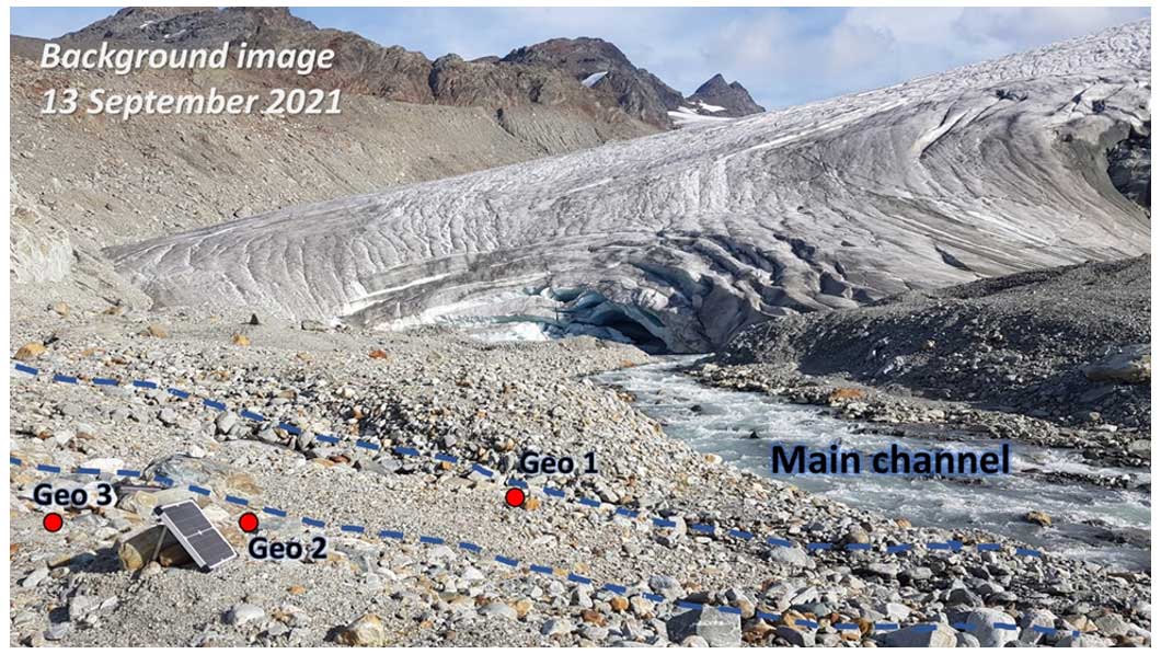
Figure 6View of the monitored reach of the proglacial stream draining the eastern tongue of Rutor Glacier. Red dots indicate the location of the geophones; the dashed blue lines denote the limits of the ephemeral stream flowing into the main channel.
The counts exported by the DATA-CUBE3 are converted to vertical ground velocity, considering the logger and geophone sensitivities according to the specifications of the manufacturer. The power spectral density is determined as the ratio of the square of the absolute value of the Fourier transform to the time window (Bakker et al., 2020). Raw seismic signals were filtered in the 5–95 Hz band, and the envelope was then calculated as the average of the absolute value of the filtered signal over a time window of 1 min.
During the 2022 season, we performed direct measurements of bedload transport at the glacier mouth by means of portable samplers during a day of intense glacier melt (14 July) and at the end of the monitoring season (16 September). Bedload traps (4 mm mesh size, 20 cm × 30 cm opening; Bunte et al., 2004) were deployed simultaneously at two positions. Measured unit bedload rates feature a large variability, ranging from 0.02 to 16.2 kg m−1 min−1 in a few hours, as has already been observed in glacierized basins (Coviello et al., 2022). Bedload samples were sieved and weighed to obtain the grain size distribution. The total bedload transport rate (Qs, kg min−1 above 4 mm) for each sampling period (ranging from 2 to 30 min) was estimated as width-weighted averages based on the available positions sampled.
The dataset derived from the results presented in the following sections is also accessible in the WebGIS mentioned above, via which it is also possible to find the link to the open repository according to the location of the monitored/surveyed point.
3.1 Orthophotos and DSM products
As described in Sect. 2.3, both aerial and UAV photogrammetric data have been processed to generate orthoimages and DSMs to support glacier monitoring from a multidisciplinary perspective.
The 2021 UAV orthoimages and DSMs are characterized by a spatial resolution lower than 4 cm: the mosaic of such metric products provides a very detailed model of the area covering the path of the water melted from the eastern glacier tongue towards the proglacial lakes (see Fig. 7b). The spatial resolution of the 2020 and 2021 aerial orthoimages is slightly lower (around 7 cm) compared with UAV imagery, while the aerial DSMs have a resolution of about 20 cm. Figure 7 clearly shows the larger coverage of the aerial orthoimage (panel a) with respect to the UAV one (panel b). As previously mentioned, the limited coverage of the UAV products is the main reason why the elevation change analysis is based on the aerial DSMs only. Nevertheless, UAV orthoimagery has been used (in addition to support the geophysical and hydraulic analyses) to assess the planimetric retreat of the eastern glacial front. More specifically, a multitemporal orthoimage comparison was performed using the photogrammetric products described above and considering the following additional datasets: (a) the 2012 color orthomosaic available as a Web Map Service (WMS) through the Italian national geoportal (http://www.pcn.minambiente.it/mattm/, last access: 23 February 2024) and (b) a Pléiades orthophoto acquired in August 2017. Figure 8 shows that the front is receding annually: the glacier tongue front has receded by more than 200 m in 9 years and by about 100 m from 2017 to 2021.
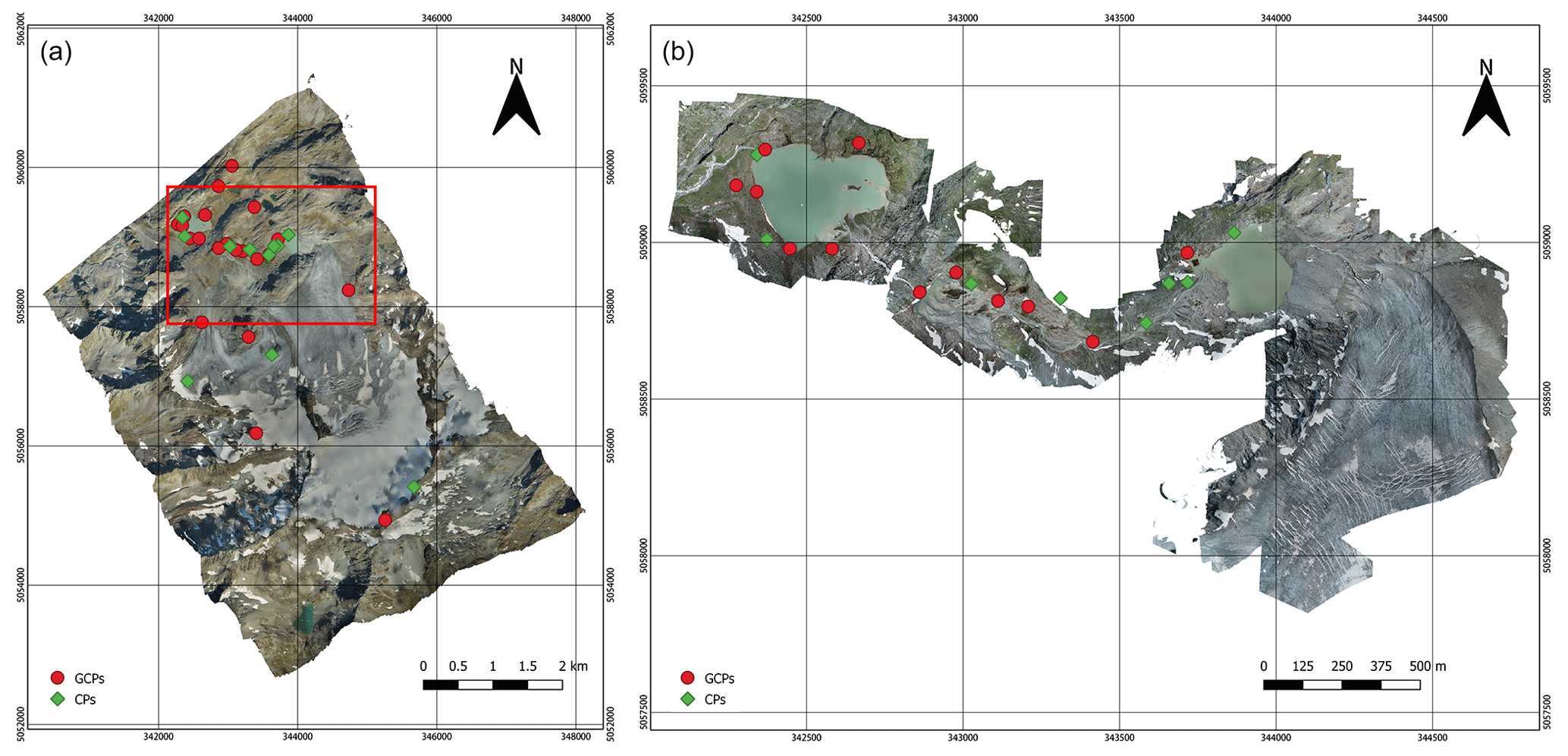
Figure 7Aerial orthophoto as of September 2021 (a) and a high-resolution UAV mosaic of orthophotos of 9 and 21 July 2021 (b).
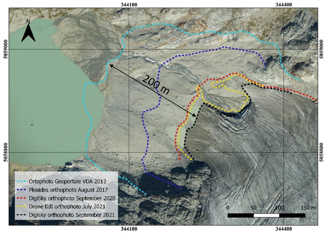
Figure 8Multitemporal analysis of the eastern glacial front retreat: front lines plotted on the September 2021 orthophoto.
3.2 DoD analysis and LoD estimation
Glacier surface elevation differences were estimated by subtracting the 2020 aerial DSM from the 2021 one in order to quantify glacier ablation and displacement (Fig. 9). Using the approach described in Sect. 2.3.1, means and standard deviations of the residuals ΔX, ΔY, and ΔZ have been computed for both GCPs and CPs (Table 5), enabling one to evaluate the planimetric and altimetric accuracies and precision of the photogrammetric products.
Table 5Means and standard deviations of the residuals ΔX, ΔY, and ΔZ calculated on GCPs and CPs. Values of interest for estimating the LoDs of the DoDs between aerial photogrammetric data from 2021 and 2020 are highlighted in bold.
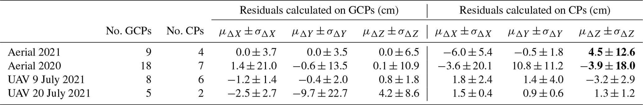
From Table 5, the mean value of ΔZ calculated on CPs (which is expected to be close to zero, being related to residuals) is not significant, even at a 68 % probability (1σ), as it is lower than the value of the ΔZ standard deviation. This suggests the absence of altimetric systematic errors for both DSMs. The planimetric error exhibits weak significance, which can be partially attributed to the precision of marker collimation. Given the good altimetric accuracy and precision achieved, it was not deemed necessary to make planimetric corrections. Referring to the previously described formulas, the value of the LoD for the DoD at a 68 % probability (1σ) is 22 cm:
Under the assumption of normality of the distribution, it becomes 44 cm (2σ) at a 95 % probability:
We are aware that this value is derived from a limited sample of CPs (Table 5, third column). However, practically speaking, it is not feasible to increase the number of points significantly due to the difficulties, time constraints, and hazards of a high-mountain environment, as previously described. Even with considerable time and effort, the number of CPs could only vary by a few units.
Nevertheless, we also tested the stable-terrain-based approach, identifying three polygons (outlined in black in Fig. 9a) corresponding to an approximately 1 km2 area downstream of the glacier fronts. These polygons were identified through the photointerpretation of aerial orthophotos and field experience to exclude local variations in the terrain, specifically those related to fluvial dynamics (all periglacial lakes and water-covered surfaces were excluded). As outlined, the statistical calculations (outlined in Table 6) were conducted both across the entire dataset and with the exclusion of the top and bottom 5 % of the distribution to mitigate any potential outliers. The mean and root-mean-square values computed over 95 % of the dataset (approximately 45 million points) exhibit a marginal decrease compared with those calculated across the entire dataset. This suggests the accurate identification of stable areas and the limited presence of outliers, a notion further supported by the similarity between the mean and median values (within a range of approximately 4 cm). Furthermore, the Fisher indices γ and γ2, which quantify skewness and kurtosis, respectively, converge towards 0 (with a probability close to 1), indicating a distribution of the DoD that approximates normality.
Table 6Statistical analysis of the DoD distribution between aerial DSMs for the years 2021 and 2020 in stable terrain.
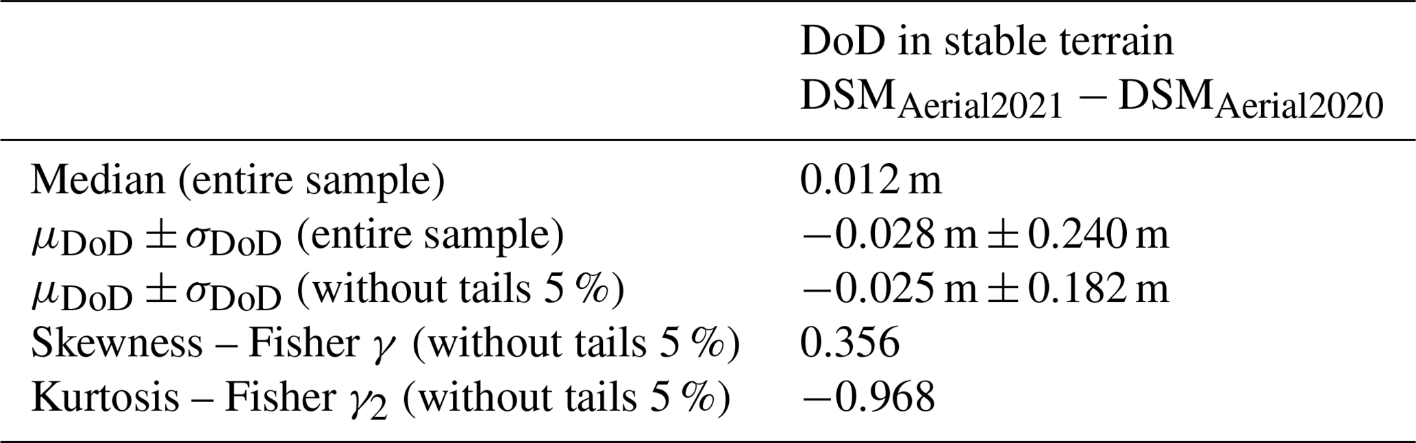
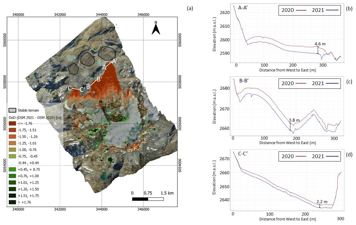
Figure 9(a) The 2021–2020 DoD; the white lines refer to the cross-sections A–A’, B–B', and C–C', whose 2020 (red) and 2021 (blue) elevation profiles are shown in panels (b), (c), and (d), respectively.
Excluding the top and bottom 5 % of the distribution and referring to the previously described formulas, the value of the LoD for the DoD at a 68 % probability (1σ) is 18 cm. Having confirmed the normality of the distribution, it becomes 36 cm (2σ) at a 95 % probability:
Taking a cautious approach and recognizing the challenge of identifying uniformly distributed stable areas across the entire surveyed region, this study has opted to use the LoD value derived from CP analysis, which stands at 44 cm (slightly higher than that obtained from stable areas). It is worth noting, however, that if representative stable areas covering the entire monitored region could be identified, the corresponding estimation of the LoD for the DoD would be considered more robust than the CP-based approach, as it would be derived from a highly representative sample of the DoD population over an area of approximately 1 km2. The DoD derived from the photogrammetric flights in 2021 and 2020 are illustrated in Fig. 9a using color intervals. To ensure clarity, a color scale with 25 cm intervals (approximately matching the DoD precision) was selected. Notably, values falling within the range from −44 to +44 cm are omitted from the figure, as they fall within the LoD for the DoD calculated based on CPs. It is apparent that the phenomenon of annual melting is less pronounced at higher elevations, where snow accumulation persists (indicated by positive DoD values in greenish colors), and becomes more prominent downstream, particularly at the glacier fronts (indicated by negative DoD values in reddish colors). These differences can reach more than 4 m, as also demonstrated by profile A–A' traced along the eastern glacier front (see Fig. 9b).
3.3 Bathymetry and lake bed sediment distribution
The outcome of the GPR survey is a series of georeferenced x-depth sections of the lake. The radar reflections depict two main interfaces: the water–fine-sediment interface, which represents the lake bottom, and a second deeper interface, which separates the fine sediments from the underlying ground layer. In the example in Fig. 10, the first (lake bottom) interface starts at a near-zero depth at the left border of the panel, deepening until 250 ns (3.5 m) in the center of the panel, and then ascending to 0 m depth in the right part of the panel. The average water depth of the lake was 3.9 m and the maximum depth was around 11 m in July 2021.
The deeper interface in Fig. 10 is fairly distinguishable and runs parallel to the first interface, deepening until 350 ns. On the left and in the center of the panel, the sediment thickness is more than twice that on the right-hand side of the panel. Under the second interface, many sparse reflections are visible; thus, the underlying layer is probably not formed by compact rock but, rather, by coarse debris or sediments. The second deeper interface was interpreted as the bottom of the fine-sediment layer. To convert the radar two-way travel times to the thickness of this layer, we needed an estimation of the signal propagation velocity in the fine sediments.
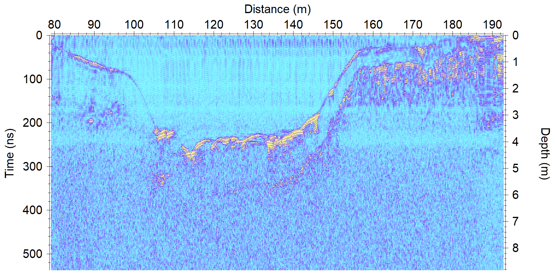
Figure 10Example of a GPR section of Lake Seracchi. Relevant reflections are the water–fine-sediment interface and, deeper, the fine-sediment–coarse-sediment interface).
The TDR probe measured a fairly uniform average relative electrical permittivity of 36±3, which was converted to a propagation velocity of about 0.05 m ns−1. Similarly to bathymetry, an interpolation process produced a final map of the thickness distribution. Figure 11 shows that major sediment accumulation has happened in the zones near the glacier inflows (from the southeast). Aside from this, the fine-sediment layer is quite homogeneously distributed all around the lake, with an average thickness of 1.6 m. Unfortunately, the zones where the water was deeper than 6–7 m could not be penetrated with sufficient energy, and the second interface was lost. This depth of investigation is the main limitation of the GPR survey and restricts the range of GPR applicability to other proglacial lakes. We expect that even the first interface could no longer be detected after 15 m of depth under similar conditions (200 MHz antenna, low-conductivity water).
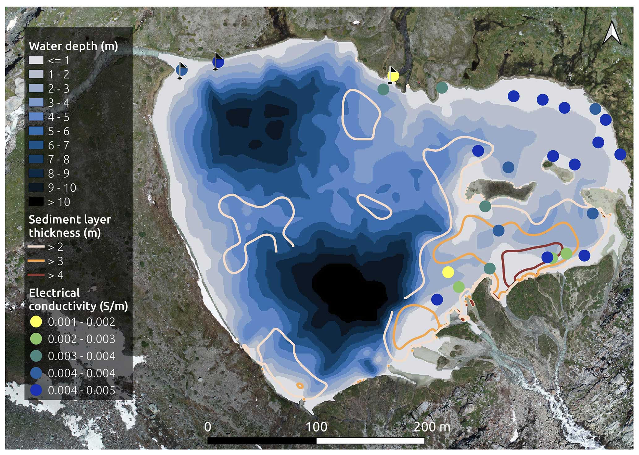
Figure 11Results of the GPR and TDR geophysical survey. The bathymetry of the lake is shown using a blue color scale. The brown contour lines indicate the areas where the sediment layer is thicker (in particular, near the inflows from the glacier). The yellow–blue points indicate the TDR measurements of electrical conductivity. The electrical permittivity is not shown here, but it is fairly uniform (average of 36). The three black flags indicate the manual sediment sampling locations. The color scale is presented as in Crameri et al. (2020).
In addition to the permittivity, the TDR probe also measured the electrical conductivity of the sediments. The locations of measurements, which also correspond to the permittivity measurements, are shown in Fig. 10. This property had a uniform value, except in small areas near the inflows. This means that the type of sediment in those zones is different from the rest of the lake. Thanks to sediment sampling (locations in Fig. 10) and grain size distribution analysis, as well as the electrical conductivity distribution, we established (via reconstruction) that the fine-sediment layer is fairly uniform around the lake and contains around 50 % clayish-sized material; in contrast, near the inflows, there is coarser gravel because the flow velocity does not allow the fine particles to sediment.
3.4 Hydrometric monitoring
The investigation at the L4 gauging station involved the following: (i) a set of 9 velocity-based discharge measurements, which allowed the stage–discharge diagram (h–Q) to be assessed, and (ii) a set of 15 elevation difference measurements, which led to the linear fit (h–H) and the lake outflow curve (H–Q) (Fig. 5).
Thanks to these results, it was possible to reconstruct the high-resolution (10 min acquisition time) temporal sequence of discharge flowing from the lake and primarily driven by the glacier melt. Figure 12a shows this temporal sequence.
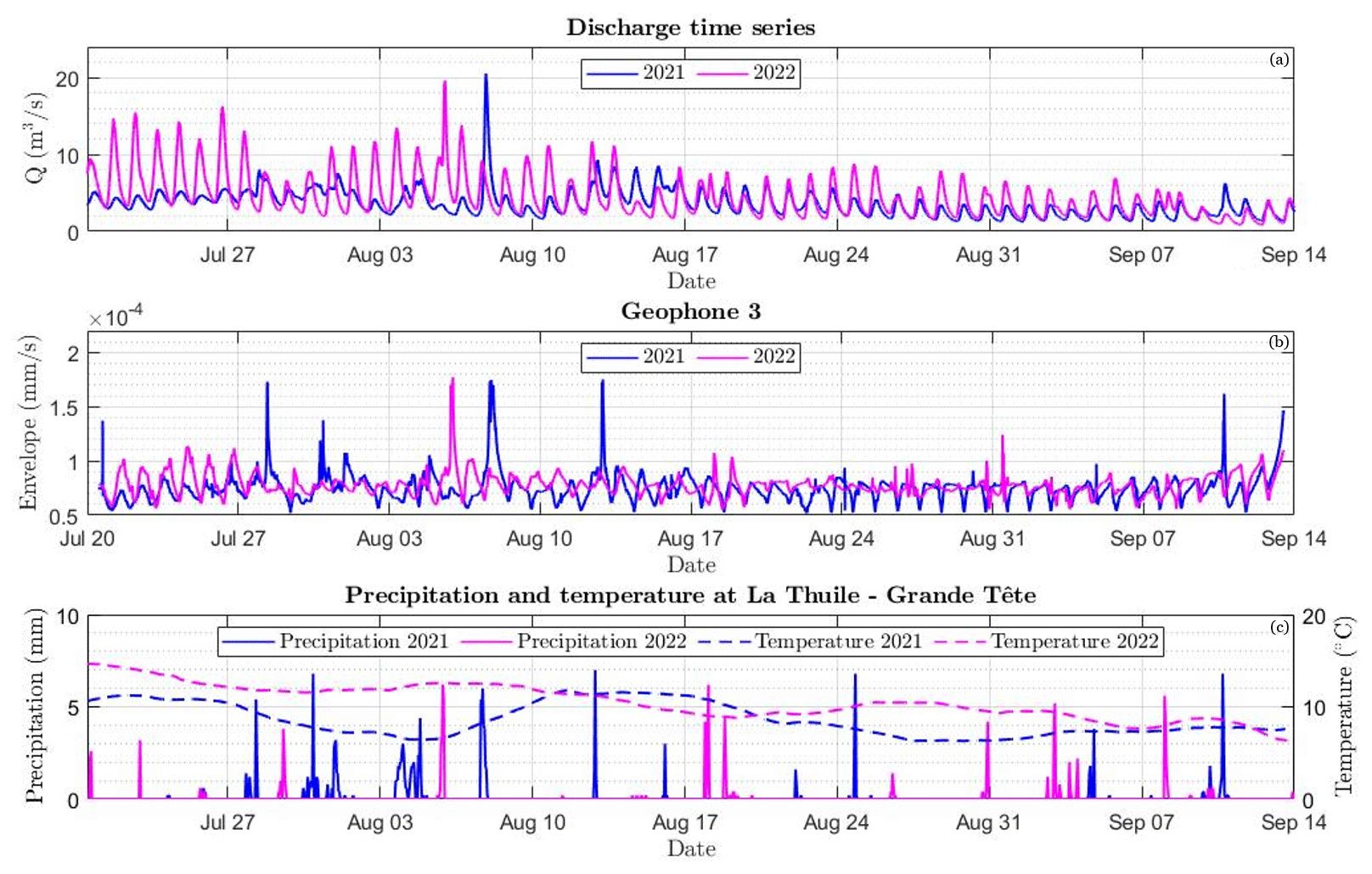
Figure 12(a) Discharge time series in the L4 emissary in 2021 and 2022. (b) Geo 3 signal envelope in 2021 and 2022 calculated using a time window of 1 min. (c) Daily precipitation (solid line) and 10 d moving mean of air temperature (dot-dash lines) measured at La Thuile-Grande Tête weather station in 2021 and 2022.
Using meteorological data from the Grande Tête weather station managed by ARPA-Valle d'Aosta (data available at https://presidi2.regione.vda.it/str_dataview_download, last access: 19 January 2023), we observed that the water level and water temperature are strongly correlated with air temperature and that this correlation is higher in summer. The summer of 2022 was warmer than that of 2021. Consequently, the average flow measured in July and August at the L4 outfall in 2022 was higher than that measured in 2021 for the same period (by as much as 26 %). The difference between the amplitude of the water level fluctuation in 2022 and 2021 was more pronounced in early summer (Fig. 12a), due to the different air temperature in May, which was 5 °C higher on average in 2022 than in 2021 (Fig. 12b), and to an earlier discharge of meltwater in 2022 than in the previous year.
The water discharge caused by glacier melt has a strong daily periodicity driven by solar radiation and thermal energy, perturbed occasionally by rainfall events. Unlike the contribution of glacier melt to water discharge, the contribution of rainfall is not periodic within the day, thus altering the otherwise daily periodic flow pattern in glacier-fed watercourses. The autocorrelation functions of the water depth time series measured at L4 and L2 highlight the daily periodicity that is strongly related to the glacier melt (Fig. 13a, b). However, the amplitude of these functions in 2021 is smaller than in 2022, and their daily means cross the zero axis earlier (about 5 d in L4 and 2 d in L2). This fact can be attributed to the different magnitude and frequency of precipitation events in the 2 years (Fig. 12). Rainfall in 2021 was more frequent than in 2022, and the July–August cumulative rainfall was 238.6 and 82.6 mm in 2021 and 2022, respectively. Accordingly, as the frequency of precipitation increases, the autocorrelation function decreases.
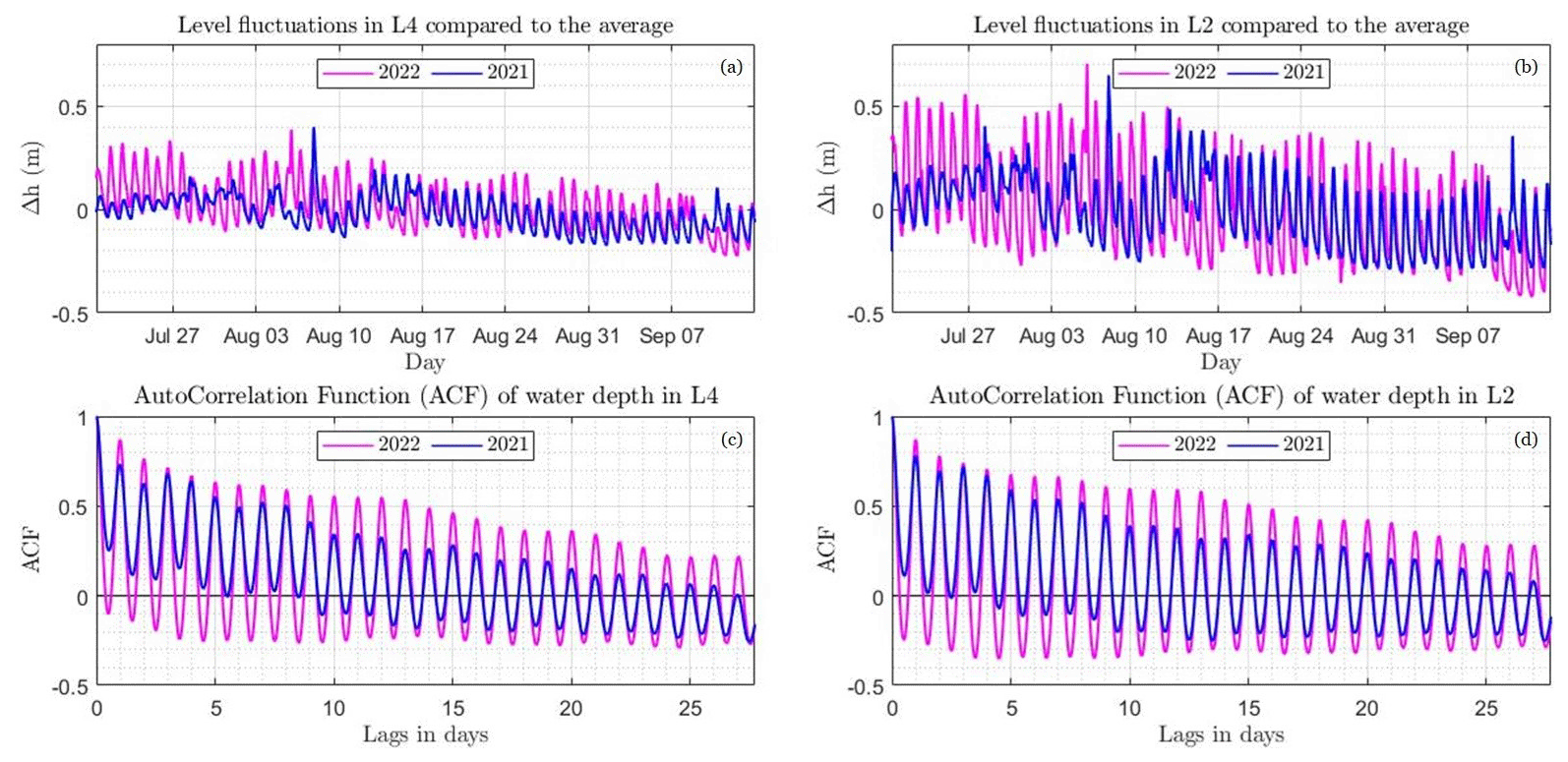
Figure 13Level fluctuations recorded in 2021 (blue) and 2022 (magenta) by measuring stations L4 (a) and L2 (b); the corresponding autocorrelation functions are shown in panels (c) and (d), respectively.
3.5 Bedload monitoring
Preliminary results show how an array of single-component geophones installed close to the flow path can detect both daily and longer-term fluctuations in bedload and water flow. The geophone signal mirrors the flow of daily cycles well, with fluctuations within a period of 24 h, and permits the identification of time intervals characterized by intense transport (Fig. 12b). Results highlight the signal fluctuations and suggest that intense runoff with bedload transport occurred during specific days (i.e., 13 July, 28 July, 4 August, 7 August, and 12–13 August). A larger flood event was detected on 7 August 2021 (Fig. 14), during which a marked increase in the seismic power was observed (i.e., 1 order of magnitude) compared with time periods characterized by low water flow and no bedload transport.
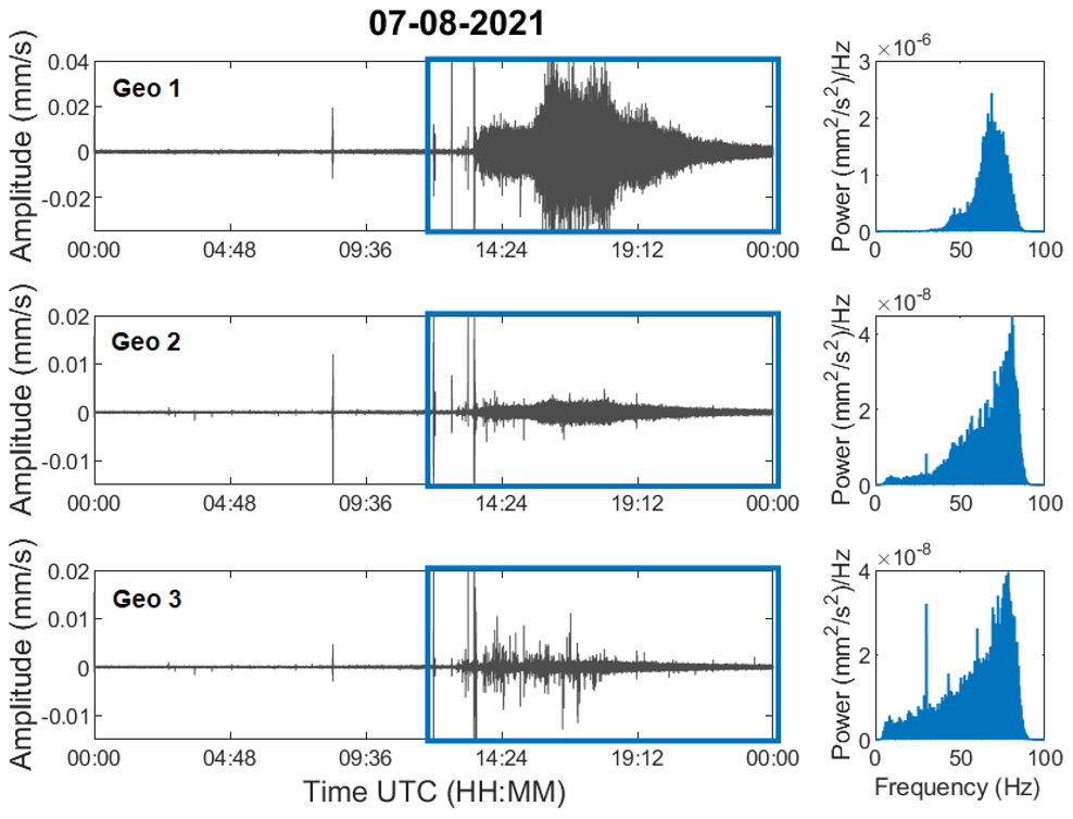
Figure 14Waveforms recorded on 7 August 2021 and power spectra of a specific portion of the signal (blue boxes, from noon to midnight UTC).
It is assumed that the geophone signal (Fig. 12b) permits the identification of time intervals characterized by intense transport, as (in correspondence with the peaks of the envelope) the power increases for high frequency values (Fig. 14). Indeed, the power in the lower bands is attributed to turbulent fluid flow (Schmandt et al., 2013), whereas that in the higher bands is attributed to bedload (Schmandt et al., 2013; Bakker et al., 2020).
In 2021, we observed, via direct inspection of the flow field, the absence of bedload transport on 3 d (10 July, 20 July, and 13 September). The dataset of direct measurements will be expanded in the future and used to calibrate the seismic data and extract quantitative information on the bedload export from the glacier.
Eight different datasets were produced. These datasets are listed below and are accessible via a WebGIS (available at https://arcg.is/Tyeju0, last access: 4 July 2024):
-
the orthophotos and DSMs related to the 2020 aerial survey are available on Zenodo at https://doi.org/10.5281/zenodo.8089499 (Corte et al., 2023c);
-
the orthophotos and DSMs related to the 2021 aerial survey are available on Zenodo at https://doi.org/10.5281/zenodo.10100968 (Corte et al., 2023f);
-
the orthophotos and DSMs related to the 2021 UAV survey is available on Zenodo at https://doi.org/10.5281/zenodo.10074530 (Corte et al., 2023g);
-
the Rutor Glacier surface area database obtained from the orthophoto of September 2021 is available on Zenodo at https://doi.org/10.5281/zenodo.10101236 (Corte et al., 2023h);
-
the footprints of the various glacial fronts obtained from the elaborated cartographic products are available on Zenodo at https://doi.org/10.5281/zenodo.7713146 (Corte et al., 2023b);
-
the bathymetry and sediment thickness of L4 database is available on Zenodo at https://doi.org/10.5281/zenodo.7682072 (Corte et al., 2023a);
-
the water depth measured by the instruments installed at gauging stations L1, L2, L3, and L4 and the relationship between the water depth and the wetted area at gauging station L4 are available on Zenodo at https://doi.org/10.5281/zenodo.7697100 (Corte et al., 2023d);
-
the geophone monitoring database is available on Zenodo at https://doi.org/10.5281/zenodo.7708800 (Corte et al., 2023e).
The images employed for the creation of the photogrammetric products used for the DoD analysis are not available in the datasets due to licensing restrictions. The ownership of the images is not exclusive to the authors but is shared with the organization responsible for their acquisition, Digisky. For this reason, it is not possible to share this dataset. To obtain the images, the purposes of the request need to be analyzed, and an agreement regarding their use must be signed directly with the authors and Digisky. We are open to sharing the dataset if it is agreed upon by Digisky.
Our objective is to increase and update the dataset by continuing to monitor and survey Rutor Glacier and its proglacial area in the future using this multidisciplinary approach.
At present (to the best of our knowledge), there appears to be a lack of work in the literature on proglacial areas involving multitemporal geospatial surveys with continuous monitoring of meltwater runoff during the ablation period, thereby merging the contributions of different disciplines. At the same time, very few cases of continuous monitoring of streamflow at high frequency and high altitude exist.
In this study, a multidisciplinary and multitemporal approach was presented to characterize Rutor Glacier and its proglacial area. Multidisciplinary analyses are fundamental in the study of complex environments. It is instructive to summarize some direct examples of the synergies involved in a multidisciplinary approach for the investigated area. Firstly, the comparison of multitemporal 3D geospatial data (taking the related DoD LoD into account) determined that the eastern tongue is losing mass faster than the others, leading to the intensification of measurements at L1 and near the eastern tongue of the glacier. Secondly, the orthoimage based on the photogrammetric UAV surveys carried out at the same time as the geophysical survey enabled the accurate extraction of the lake perimeter, which – integrated with the data acquired from the GPR – resulted in an accurate bathymetry of the lake and allowed one to establish the exact outline of the zero-depth points at the time of the investigation. Thirdly, continuous hydraulic monitoring at the L4 gauging station and the relationship between the water depth measured by the sensor and the depth of the lake provided the volume change in L4 over time. In addition, combining the bathymetry map with the DSM of the surrounding area will enable the determination of the water volume of L4 when the water level is higher than at the time of the geophysical survey. Lastly, the extracted products of the crewed aerial photogrammetric flights allowed the environmental agency (ARPA-Valle d'Aosta) to develop the mass balance for the hydrological years under consideration. The comparison of different DSMs sets the basis for continuous monitoring over time, in which the 2021 model will serve as a reference for future comparisons. The mass balance of Rutor Glacier can also be determined through the application of a hydrological model calibrated with the water discharge time series obtained from this study. It is important to stress that the accurate georeferencing of all of the acquired data with respect to the same datum plays a crucial role in the data integration phase and in enabling multitemporal analyses.
Future modeling of the water flow and sediment transport at L4 may be based on the bathymetry map combined with the inflow and outflow measurements. The GPR and TDR surveys, with a few ground-proof sediment samples, evidenced that a fine-sediment layer that is 1.6 m thick on average has been deposited on the lake bottom in the approximate 140 years since the birth of the lake. Sediment transport deserves further investigation, as it may change due to the rapid shrinking of Rutor Glacier, whose bedrock erosion is the source of the fine sediment found in the lake. An approach to modeling these changes could involve the temporal monitoring of water turbidity as a proxy for the concentration of suspended sediment in the various inflows and outflows of the interconnected waterbodies.
The multidisciplinary approach and the dataset presented herein enable the characterization, monitoring, and understanding of a set of complex processes that take place in the study area, allowing the authors to shed light on interconnected phenomena with a broader perspective than a single-scientific-discipline approach. Indeed, the results of a combined effort often go beyond the sum of each contribution.
The procedure followed to measure the velocity is reported in ISO 748:2007. The methods used to determine the discharge from current meter measurements are classified in ISO 748:2007 as the graphical method and the arithmetic method. The latter, which is more suitable for computations carried out in the field, includes two methods: the mean-section method and the mid-section method. The discharge was determined by applying both arithmetic methods and averaging the two results.
The power law is the one that best represents the stage–discharge measurements (Fig. 5):
The lowest water discharge measured corresponds to a water depth in the cross-section of 0.49 m. In fact, the power law describes the Q–h relationship well when h is greater than 0.5 m. For shallower water depths, the power law returns a flow rate that is too low for the geometry of the cross-section considered. Consequently, for h<0.49 m, the stage–discharge curve was obtained by taking the geometry of the cross-section into account.
Water discharge can be written as a function of the wetted area of the cross-section:
where Q is the discharge, k is a flow resistance coefficient, Ω is the wetted area, and m is a coefficient dependent on the cross-section geometry. To obtain the expression of the coefficient m, the stage–discharge relationship and Chézy equation were expanded using the Taylor series and set equal to each other, thereby obtaining the following:
This coefficient depends on the wetted area (Ω) and the wetted perimeter (B) of the cross-section.
The geometry of the cross-section of L4's emissary was determined through an RTK survey. The measurements of the three coordinates of the points within the cross-section bed were with steps of about 20 cm along the cross-direction.
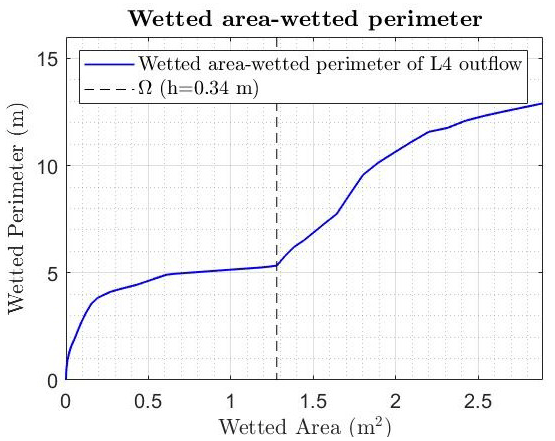
Figure A1The wetted area and the corresponding wetted perimeter for water depths between h=0 and h=52 cm.
When visualizing the cross-section geometry and the curve that describes how the wet perimeter changes with the wet area (Fig. A1), it is clear that two different stage–discharge relationships, corresponding to two different water depth intervals, must be considered:
For each interval, the coefficient m was calculated as the mean of all of the values determined at each point within the corresponding interval. Considering the first interval from h1 to hn and the second from hn+1 to hl, the coefficients were calculated according to the following expressions:
The k coefficients were calculated by imposing the continuity stage–discharge relationship at h=0.34 cm and h=0.49 cm, respectively, thereby obtaining k1=0.232 and k2=0.257, respectively. The definitive stage–discharge relationship is given by three different relationships corresponding to three different water depth intervals:
Following this operation, it is possible to verify whether the median, a robust estimator, and mean of the DoD are similar (an indicator of the absence of outliers) and to assess the normality of the distribution. The test for normality of a sample of observations can be conducted by considering the kth-order moments relative to the mean of the deviation variable:
With k=3, the moment is termed skewness; with k=4, the moment is termed kurtosis. These values provide information on the asymmetry and peakedness of the distribution under examination, relative to the normal distribution. With these properties, we can define the Fisher indices by considering the following:
-
the skewness coefficient,
-
the kurtosis coefficient,
If the distribution approaches normality, these coefficients tend towards zero. We can evaluate their proximity to zero by testing the z scores, normalized with respect to their standard error. The null hypothesis assumes that the gamma indices are equal to zero. For the text concerning skewness, let us consider the following:
For the test concerning kurtosis, let us consider the following:
At the normalized z value, we can search for the probability of accepting the null hypothesis on tables of the normal distribution.
The GPR profiles were processed in the Reflexw software (Sandmeier, 2021) according to the following processing steps:
-
We first used “Move startime” to delete the data acquired before the radar impulse transmission. To automatically recognize the timing of the transmitted impulse, the Reflexw processing “Correct max phase” was also used.
-
“Make equidistant traces” was subsequently used to make the distance between each trace 0.1 m, in order to compensate for the variable speed of the boat.
-
We then employed “subtract mean – dewow”, a filter that subtracted the average of a trace from each trace, on a 5 ns time window, to correct for instrumental voltage shifts.
-
Next, “Bandpass butterworth”, a bandpass filter that cut the frequencies lower than 50 MHz and higher than 260 MHz, was implemented.
-
Then, “subtracting average”, a filter that subtracts the average trace from each trace within a 100-trace window, was employed to eliminate horizontally coherent noise.
-
Finally, “energy decay”, a simple time-axis gain function that equalizes the energy of the traces, which generally decreases over time, was used.
The supplement related to this article is available online at: https://doi.org/10.5194/essd-16-3283-2024-supplement.
AC, CC, AG, and ST: conceptualization and supervision; EC, VC, MMM, and AV: data curation; AA, EC, MMM, FGT, and AV: visualization; EC (with contributions from all co-authors): manuscript preparation; all authors: investigation.
The contact author has declared that none of the authors has any competing interests.
Publisher’s note: Copernicus Publications remains neutral with regard to jurisdictional claims made in the text, published maps, institutional affiliations, or any other geographical representation in this paper. While Copernicus Publications makes every effort to include appropriate place names, the final responsibility lies with the authors.
The authors thank Umberto Morra di Cella (ARPA-Valle d’Aosta) for his collaboration and interesting discussions; Francesco Comiti and Matthias Bonfrisco (Free University of Bozen-Bolzano) for supporting bedload measurements; and Paolo Maschio and Nives Grasso for supporting UAV acquisitions. We are also grateful to the Italian Ministry for Education and Research (MIUR) for the award granted through the “Department of Excellence 2018–2022” project to the Department of Environment, Land, and Infrastructure Engineering (DIATI) at the Polytechnic University of Turin, which was used to finance part of the installed equipment and the crewed aerial photogrammetric flights.
This research has been supported by the European Regional Development Fund, Interreg (grant no. 8504).
This paper was edited by James Thornton and reviewed by three anonymous referees.
Alley, R., Cuffey, K., Evenson, E., Strasser, J., Lawson, D., and Larson, G.: How glaciers entrain and transport basal sediment: Physical constraints, Quaternary Sci. Rev., 16, 1017–1038, https://doi.org/10.1016/S0277-3791(97)00034-6, 1997. a
ARPA Valle d'Aosta: Bilancio di massa, ARPA Valle d'Aosta, Tech. Rep., Agenzia Regionale Protezione Ambiente Valle d'Aosta, https://www.arpa.vda.it/it/effetti-sul-territorio-dei-cambiamenti-climatici/ghiacciai/bilancio-di-massa (last access: 3 July 2024), 2014. a
Bakker, M., Gimbert, F., Geay, T., Misset, C., Zanker, S., and Recking, A.: Field Application and Validation of a Seismic Bedload Transport Model, J. Geophys. Res.-Earth, 125, e2019JF005416, https://doi.org/10.1029/2019JF005416, 2020. a, b, c
Baretti, M.: Il Lago del Rutor (Alpi Graje settentrionali), Bollettino del “Club Alpino Italiano”, 14, 43–98, https://tecadigitale.cai.it/periodici/PDF/Bollettino/ (last access: 4 July 2024), 1880. a, b
Bogen, J., Xu, M., and Kennie, P.: The impact of pro‐glacial lakes on downstream sediment delivery in Norway, Earth Surf. Process. Landf., 40, 942–952, https://doi.org/10.1002/esp.3669, 2015. a
Bradford, J. H., Johnson, C. R., Brosten, T., McNamara, J. P., and Gooseff, M. N.: Imaging thermal stratigraphy in freshwater lakes using georadar, Geophys. Res. Lett., 34, L24405, https://doi.org/10.1029/2007GL032488, 2007. a
Brasington, J., Rumsby, B. T., and McVey, R. A.: Monitoring and modelling morphological change in a braided gravel-bed river using high resolution GPS-based survey, Earth Surf. Process. Landf., 25, 973–990, https://doi.org/10.1002/1096-9837(200008)25:9<973::AID-ESP111>3.0.CO;2-Y, 2000. a
Bunte, K., Abt, S. R., Potyondy, J. P., and Ryan, S. E.: Measurement of Coarse Gravel and Cobble Transport Using Portable Bedload Traps, J. Hydraul. Eng.-ASCE, 130, 879–893, https://doi.org/10.1061/(ASCE)0733-9429(2004)130:9(879), 2004. a
Camporese, M., Penna, D., Borga, M., and Paniconi, C.: A field and modeling study of nonlinear storage-discharge dynamics for an Alpine headwater catchment, Water Resour. Res., 50, 806–822, 2014. a
Carrer, M., Dibona, R., Prendin, A. L., and Brunetti, M.: Recent waning snowpack in the Alps is unprecedented in the last six centuries, Nat. Clim. Change, 13, 155–160, https://doi.org/10.1038/s41558-022-01575-3, 2023. a
Carrivick, J. L. and Tweed, F. S.: Deglaciation controls on sediment yield: Towards capturing spatio-temporal variability, Earth-Sci. Rev., 221, 103809, https://doi.org/10.1016/j.earscirev.2021.103809, 2021. a, b, c
Cavalli, M., Heckmann, T., and Marchi, L.: Sediment Connectivity in Proglacial Areas, Geography of the Physical Environment, Springer International Publishing, Cham, 271–287, ISBN 9783319941820, 2018. a
Chiabrando, F., Giulio Tonolo, F., and Lingua, A.: UAV Direct Georeferencing Approach in an Emergency Mapping Context. The 2016 Central Italy Earthquake Case Study, Int. Arch. Photogramm. Remote Sens. Spatial Inf. Sci., XLII-2/W13, 247–253, https://doi.org/10.5194/isprs-archives-XLII-2-W13-247-2019, 2019. a
Corte, E., Ajmar, A., Camporeale, C., Cina, A., Coviello, V., Giulio Tonolo, F., Godio, A., Macelloni, M. M., Oggeri, C., Tamea, S., and Vergnano, A.: Bathymetry, sediment thickness, and geotechnical-geophysical properties of sediments of Lake Seracchi in Rutor proglacial area, Zenodo [data set], https://doi.org/10.5281/zenodo.7682072, 2023a. a, b
Corte, E., Ajmar, A., Camporeale, C., Cina, A., Coviello, V., Giulio Tonolo, F., Godio, A., Macelloni, M. M., Tamea, S., and Vergnano, A.: Rutor glacier fronts footprints, Zenodo [data set], https://doi.org/10.5281/zenodo.7713146, 2023b. a, b
Corte, E., Ajmar, A., Camporeale, C., Cina, A., Coviello, V., Giulio Tonolo, F., Godio, A., Macelloni, M. M., Tamea, S., and Vergnano, A.: Orthophoto and DSM Rutor Glacier 2020, Zenodo [data set], https://doi.org/10.5281/zenodo.8089499, 2023c. a, b
Corte, E., Ajmar, A., Camporeale, C., Cina, A., Coviello, V., Giulio Tonolo, F., Godio, A., Macelloni, M. M., Tamea, S., and Vergnano, A.: Hydrometric data in the Rutor proglacial area, Zenodo [data set], https://doi.org/10.5281/zenodo.7697100, 2023d. a, b
Corte, E., Ajmar, A., Camporeale, C., Cina, A., Coviello, V., Giulio Tonolo, F., Godio, A., Macelloni, M. M., Tamea, S., Vergnano, A., Bonfrisco, M., and Comiti, F.: Geophone data in the Rutor proglacial area (Valle d’Aosta, Italy), Zenodo [data set], https://doi.org/10.5281/zenodo.7708800, 2023e. a, b
Corte, E., Ajmar, A., Camporeale, C., Cina, A., Coviello, V., Giulio Tonolo, F., Godio, A., Macelloni, M. M., Tamea, S., and Vergnano, A.: Orthophoto and DSM Rutor Glacier 2021, Zenodo [data set], https://doi.org/10.5281/zenodo.10100968, 2023f. a, b
Corte, E., Ajmar, A., Camporeale, C., Cina, A., Coviello, V., Giulio Tonolo, F., Godio, A., Macelloni, M. M., Tamea, S., and Vergnano, A.: Ortophotos and DSMs UAV, Zenodo [data set], https://doi.org/10.5281/zenodo.10074530, 2023g. a, b
Corte, E., Ajmar, A., Camporeale, C., Cina, A., Coviello, V., Giulio Tonolo, F., Godio, A., Macelloni, M. M., Tamea, S., and Vergnano, A.: Rutor Glacier Surface Area – 2021, Zenodo [data set], https://doi.org/10.5281/zenodo.10101236, 2023h. a, b
Corte, E., Ajmar, A., Camporeale, C., Cina, A., Coviello, V., Giulio Tonolo, F., Godio, A., Macelloni, M. M., Tamea, S., and Vergnano, A.: Photogrammetric processing reports for two crewed aerial flights over the Rutor Glacier, Zenodo [data set], https://doi.org/10.5281/zenodo.11144390, 2024. a
Coviello, V., Capra, L., Vázquez, R., and Márquez-Ramírez, V. H.: Seismic characterization of hyperconcentrated flows in a volcanic environment, Earth Surf. Process. Landf., 43, 2219–2231, https://doi.org/10.1002/esp.4387, 2018. a
Coviello, V., Vignoli, G., Simoni, S., Bertoldi, W., Engel, M., Buter, A., Marchetti, G., Andreoli, A., Savi, S., and Comiti, F.: Bedload Fluxes in a Glacier‐Fed River at Multiple Temporal Scales, Water Resour. Res., 58, e2021WR031873, https://doi.org/10.1029/2021WR031873, 2022. a, b
Crameri, F., Shephard, G. E., and Heron, P. J.: The misuse of colour in science communication, Nat. Commun., 11, 5444, https://doi.org/10.1038/s41467-020-19160-7, 2020. a
Curry, A. M., Cleasby, V., and Zukowskyj, P.: Paraglacial response of steep, sediment-mantled slopes to post-“Little Ice Age” glacier recession in the central Swiss Alps, J. Quaternary Sci., 21, 211–225, https://doi.org/10.1002/jqs.954, 2006. a, b
Delaney, I., Bauder, A., Huss, M., and Weidmann, Y.: Proglacial erosion rates and processes in a glacierized catchment in the Swiss Alps, Earth Surf. Process. Landf., 43, 765–778, https://doi.org/10.1002/esp.4239, 2018. a, b
Eichel, J.: Vegetation Succession and Biogeomorphic Interactions in Glacier Forelands, pp. 327–349, Springer International Publishing, Cham, ISBN 978-3-319-94184-4, https://doi.org/10.1007/978-3-319-94184-4_19, 2019. a
Gizzi, M., Mondani, M., Suozzi, E., Glenda, T., and Lo Russo, S.: Aosta Valley Mountain Springs: A Preliminary Analysis for Understanding Variations in Water Resource Availability under Climate Change, Water, 14, 1004, https://doi.org/10.3390/w14071004, 2022. a
GLIMS Consortium: GLIMS Glacier Database, Version 1, NASA National Snow and Ice Data Center Distributed Active Archive Center [data set], https://doi.org/10.7265/N5V98602, 2005. a, b
Grove, J. M.: Little Ice Ages, Ancient and Modern: 2nd edn., Routledge, ISBN 9781134701827, https://doi.org/10.4324/9780203770269, 2004. a
Guillon, H., Mugnier, J. L., and Buoncristiani, J. F.: Proglacial sediment dynamics from daily to seasonal scales in a glaciated Alpine catchment (Bossons glacier, Mont Blanc massif, France), Earth Surf. Process. Landf., 43, 1478–1495, https://doi.org/10.1002/esp.4333, 2018. a, b, c
Hallet, B., Hunter, L., and Bogen, J.: Rates of erosion and sediment evacuation by glaciers: A review of field data and their implications, Glob. Planet. Change, 12, 213–235, https://doi.org/10.1016/0921-8181(95)00021-6, 1996. a, b
He, H., Aogu, K., Li, M., Xu, J., Sheng, W., Jones, S. B., González-Teruel, J. D., Robinson, D. A., Horton, R., Bristow, K., Dyck, M., Filipović, V., Noborio, K., Wu, Q., Jin, H., Feng, H., Si, B., and Lv, J.: A review of time domain reflectometry (TDR) applications in porous media, in: Advances in Agronomy, vol. 168, Academic Press Inc., 83–155, ISBN 9780128245897, https://doi.org/10.1016/bs.agron.2021.02.003, 2021. a
Heckmann, T. and Schwanghart, W.: Geomorphic coupling and sediment connectivity in an alpine catchment – Exploring sediment cascades using graph theory, Geomorphology, 182, 89–103, https://doi.org/10.1016/j.geomorph.2012.10.033, 2013. a
Hicks, D. M., McSaveney, M. J., and Chinn, T. J.: Sedimentation in proglacial Ivory Lake, Southern Alps, New Zealand, Arct. Alp. Res., 22, 26–42, https://doi.org/10.2307/1551718, 1990. a
Hilger, L. and Beylich, A. A.: Sediment Budgets in High-Mountain Areas: Review and Challenges, chap. 15, Springer International Publishing, Cham, 251–269, ISBN 978-3-319-94184-4, https://doi.org/10.1007/978-3-319-94184-4_15, 2019. a, b, c
Hooke, R. L.: Toward a uniform theory of clastic sediment yield in fluvial systems, GSA Bulletin, 112, 1778–1786, https://doi.org/10.1130/0016-7606(2000)112<1778:TAUTOC>2.0.CO;2, 2000. a
Ivy-Ochs, S., Kerschner, H., Maisch, M., Christl, M., Kubik, P. W., and Schlüchter, C.: Latest Pleistocene and Holocene glacier variations in the European Alps, Quaternary Sci. Rev., 28, 2137–2149, https://doi.org/10.1016/j.quascirev.2009.03.009, 2009. a
James, M., Chandler, J., Eltner, A., Fraser, C., Miller, P., Mills, J., Noble, T., Robson, S., and Lane, S.: Guidelines on the use of Structure from Motion Photogrammetry in Geomorphic Research, Earth Surf. Process. Landf., 44, 2081–2084, https://doi.org/10.1002/esp.4637, 2019. a
Lane, S. N., Westaway, R. M., and Murray Hicks, D.: Estimation of erosion and deposition volumes in a large, gravel-bed, braided river using synoptic remote sensing, Earth Surf. Process. Landf., 28, 249–271, https://doi.org/10.1002/esp.483, 2003. a
Laute, K. and Beylich, A. A.: Environmental controls, rates and mass transfers of contemporary hillslope processes in the headwaters of two glacier-connected drainage basins in western Norway, Geomorphology, 216, 93–113, https://doi.org/10.1016/j.geomorph.2014.03.021, 2014. a
Mao, L., Comiti, F., Carrillo, R., and Penna, D.: Sediment Transport in Proglacial Rivers, in: Geomorphology of Proglacial Systems, Geography of the Physical Environment, Springer International Publishing, Cham, 199–217, ISBN 9783319941820, 2018. a
Matthews, J. A.: Geomorphology of Proglacial Systems: Landform and Sediment Dynamics in Recently Deglaciated Alpine Landscapes, vol. 29, Springer Cham, ISBN 9783319941820, https://doi.org/10.1177/0959683619840576, 2019. a, b
Moreau, M., Mercier, D., Laffly, D., and Roussel, E.: Impacts of recent paraglacial dynamics on plant colonization: A case study on midtre Lovénbreen foreland, Spitsbergen (79° N), Geomorphology, 95, 48–60, https://doi.org/10.1016/j.geomorph.2006.07.031, 2008. a
Müller, B. U.: Paraglacial sedimentation and denudation processes in an Alpine valley of Switzerland. An approach to the quantification of sediment budgets, Geodin. Acta, 12, 291–301, https://doi.org/10.1016/S0985-3111(00)87046-1, 1999. a
Orombelli, G.: Il ghiacciaio del Ruitor (Valle d’Aosta) nella piccola età glaciale, Geogr. Fis. Dinam. Quat. Suppl. VII, 239–251, 2005. a
Orwin, J. F. and Smart, C. C.: Short-term spatial and temporal patterns of suspended sediment transfer in proglacial channels, small River Glacier, Canada, Hydrol. Process., 18, 1521–1542, 2004. a, b
Paul, F., Bolch, T., Briggs, K., Kääb, A., McMillan, M., McNabb, R., Nagler, T., Nuth, C., Rastner, P., Strozzi, T., and Wuite, J.: Error sources and guidelines for quality assessment of glacier area, elevation change, and velocity products derived from satellite data in the Glaciers_cci project, Remote Sens. Environ., 203, 256–275, https://doi.org/10.1016/j.rse.2017.08.038, 2017. a
Psarras, G. C.: Fundamentals of dielectric theories, in: Dielectric Polymer Materials for High-Density Energy Storage, Elsevier, 11–57, ISBN 9780128132159, https://doi.org/10.1016/B978-0-12-813215-9.00002-6, 2018. a
Raup, B., Racoviteanu, A., Khalsa, S. J. S., Helm, C., Armstrong, R., and Arnaud, Y.: The GLIMS geospatial glacier database: A new tool for studying glacier change, Glob. Planet. Change, 56, 101–110, https://doi.org/10.1016/j.gloplacha.2006.07.018, 2007. a, b
Sacco, F.: Il ghiacciaio ed i laghi del Ruitor, Bollettino della Società Geologica Italiana, 36, 1–36, https://www.socgeol.it/?sitelang=eng (last access: 15 July 2024), 1917. a, b, c
Sambuelli, L., Colombo, N., Giardino, M., and Godone, D.: A waterborne GPR survey to estimate fine sediments volume and find optimum core location in a Rockglacier Lake, in: Near Surface Geoscience 2015, in: 21st European Meeting of Environmental and Engineering Geophysics, 1, European Association of Geoscientists and Engineers, EAGE, 811–815, ISBN 9781510814127, https://doi.org/10.3997/2214-4609.201413826, 2015. a
Sandmeier, K.-J.: Reflexw, Sandmeier Geophysical Research [software], https://www.sandmeier-geo.de/index.html (last access: 4 July 2024), 2021. a, b
Schmandt, B., Aster, R. C., Scherler, D., Tsai, V. C., and Karlstrom, K.: Multiple fluvial processes detected by riverside seismic and infrasound monitoring of a controlled flood in the Grand Canyon, Geophys. Res. Lett, 40, 4858–4863, https://doi.org/10.1002/grl.50953, 2013. a, b, c
SCT Geoportale, Regione autonoma Valle d'Aosta: Regione Autonoma Valle d'Aosta, Sistema delle Conoscenze Territoriali, Geoportale, https://mappe.regione.vda.it/pub/geonavitg/geodownload.asp?carta=DSM08, last access: 4 July 2024. a, b
Slaymaker, O.: Criteria to Distinguish Between Periglacial, Proglacial and Paraglacial Environments, Quaest. Geogr., 30, 85–94, https://doi.org/10.2478/v10117-011-0008-y, 2011. a, b
Sommer, C., Malz, P., Seehaus, T., Lippl, S., Zemp, M., and Braun, M. H.: Rapid glacier retreat and downwasting throughout the European Alps in the early 21st century, Nat. Commun., 11, 3209, https://doi.org/10.1038/s41467-020-16818-0, 2020. a
Teppati Losè, L., Chiabrando, F., and Giulio Tonolo, F.: Are Measured Ground Control Points Still Required in UAV Based Large Scale Mapping? Assessing the Positional Accuracy of an RTK Multi-Rotor Platform, Int. Arch. Photogramm. Remote Sens. Spatial Inf. Sci., XLIII-B1-2020, 507–514, https://doi.org/10.5194/isprs-archives-XLIII-B1-2020-507-2020, 2020a. a
Teppati Losè, L., Chiabrando, F., and Giulio Tonolo, F.: Boosting the Timeliness of UAV Large Scale Mapping. Direct Georeferencing Approaches: Operational Strategies and Best Practices, ISPRS Int. J. Geo-Inf., 9, 578, https://doi.org/10.3390/ijgi9100578, 2020b. a
Valbusa, U. and Peretti, L.: Relazioni delle Campagne Glaciologiche del 1936, Bollettino del Comitato Glaciologico Italiano, vol. 17, p. 183, Tipografia Nazionale di G. Bertero C., 1937. a
Vergnano, A., Oggeri, C., and Godio, A.: Geophysical–geotechnical methodology for assessing the spatial distribution of glacio‐lacustrine sediments: The case history of Lake Seracchi, Earth Surf. Proc. Land., 48, 1374–1397, https://doi.org/10.1002/esp.5555, 2023. a, b, c
Villa, F., De Amicis, M., and Maggi, V.: GIS analysis of Rutor Glacier (Aosta Valley, Italy) volume and terminus variations, Geogr. Fis. Din. Quat., 30, 87–95, 2007. a, b, c, d, e
Zhang, T., Li, D., East, A. E., Walling, D. E., Lane, S., Overeem, I., Beylich, A. A., Koppes, M., and Lu, X.: Warming-driven erosion and sediment transport in cold regions, Nat. Rev. Earth Environ., 3, 832–851, https://doi.org/10.1038/s43017-022-00362-0, 2022. a
- Abstract
- Dedication
- Introduction
- Materials and methods
- Results
- Data availability
- Conclusions
- Appendix A: Stage–discharge relationship for L4
- Appendix B: Normality testing – skewness and kurtosis
- Appendix C: GPR data processing
- Author contributions
- Competing interests
- Disclaimer
- Acknowledgements
- Financial support
- Review statement
- References
- Supplement