HUST-Grace2024: a new GRACE-only gravity field time series based on more than 20 years of satellite geodesy data and a hybrid processing chain

To improve the accuracy of monthly temporal gravity field models for the Gravity Recovery and Climate Experiment (GRACE) and the GRACE Follow-On (GRACE-FO) missions, a new series named HUST-Grace2024 is determined based on the updated L1B datasets (GRACE L1B RL03 and GRACE-FO L1B RL04) and the newest atmosphere and ocean de-aliasing product (AOD1B RL07). Compared to the previous HUST temporal gravity field model releases, we have made the following improvements related to updating the background models and the processing chain: (1) during the satellite onboard events, the inter-satellite pointing angles are calculated to pinpoint outliers in the K-band ranging (KBR) range-rate and accelerometer observations. To exclude outliers, the advisable threshold is 50 mrad for KBR range rates and 20 mrad for accelerations. (2) To relieve the impacts of KBR range-rate noise at different frequencies, a hybrid data-weighting method is proposed. Kinematic empirical parameters are used to reduce the low-frequency noise, while a stochastic model is designed to relieve the impacts of random noise above 10 mHz. (3) A fully populated scale factor matrix is used to improve the quality of accelerometer calibration. Analyses in the spectral and spatial domains are then implemented, which demonstrate that HUST-Grace2024 yields a noticeable reduction of 10 % to 30 % in noise level and retains consistent amplitudes of signal content over 48 river basins compared with the official GRACE and GRACE-FO solutions. These evaluations confirm that our aforementioned efforts lead to a better temporal gravity field series. This data set is identified with the following DOI: https://doi.org/10.5880/ICGEM.2024.001 (Zhou et al., 2024).

1 Introduction

The Gravity Recovery and Climate Experiment (GRACE) mission and its follow-on mission GRACE-FO (Tapley et al., 2004; Landerer et al., 2020) provide us with an opportunity to accurately monitor mass transportation for the Earth system. The GRACE missions comprise two identical satellites, GRACE-A and GRACE-B, following each other in the same orbital track and linked by a highly accurate inter-satellite K-band microwave ranging system. The outputs of the GRACE missions are a series of monthly temporal gravity field models, represented as a series of harmonic coefficients for a specific order and degree. The variation in temporal gravity field represented as the equivalent water height can be used to monitor the mass transportation for the Earth system, including the hydrological cycle over the basins, the variation over the large glaciers, and even extreme weather events like drought or flood events (e.g., Alexander et al., 2016; Amin et al., 2020; Argus et al., 2017; Carlson et al., 2022; Gupta and Dhanya, 2020). In general, the temporal gravity field models give us new insight into large-scale mass transportation in the Earth system over decades, thus advancing the progress of geoscience.

The monthly temporal gravity field of GRACE and GRACE-FO, denoted as a level 2 (L2) product, is produced from a series of pre-processed level 1B (L1B) products, which include the GPS observation measured by onboard receivers, the attitude data observed by star cameras, the non-gravitational forces measured by accelerometers, and the range rates derived from the K- and Ka-band link between two satellites. In order to obtain the temporal gravity field models from these L1B products, a number of background models need to be added during the gravity field determination, which include the ocean tide models, atmosphere and ocean de-aliasing (AOD1B) products, and the static gravity field. The L2 products are provided by the official solution centers, which include the Center for Space Research (CSR; Bettadpur, 2018), the German Research Centre for Geosciences (GFZ; Dahle et al., 2018), and the Jet Propulsion Laboratory (JPL; Yuan, 2018). Apart from the official solution centers, there are also a series of research centers computing the monthly gravity field products, which can be found on the website of the International Centre for Global Earth Models (Ince et al., 2019).

Due to the limited knowledge of error sources for both observations and background models, the accuracy of current GRACE temporal gravity field models still cannot reach the pre-launch baseline accuracy, which is derived from a pre-launch simulation study (Kim and Tapley, 2000; Ditmar et al., 2011; Flechtner et al., 2015). In order to improve the quality of temporal gravity field models, many researchers have made numerous efforts to elucidate the error sources in the observation data and attempted to model them. For instance, several researchers have discussed the star camera noise and imposed a new combination method based on different star cameras or angular accelerometers in ACC1B and recomputed the antenna phase center corrections for the inter-satellite observations (e.g., Bandikova and Flury, 2014; Goswami et al., 2018; Horwath et al., 2010). Based on this new processing strategy, the corresponding L1B datasets for star camera attitudes (SCA1B) and K-band ranges (KBR1B) have been updated to release 03 (RL03) in our GRACE solution, while all L1B datasets for the GRACE-FO solution correspond to the newest RL04 edition. Meanwhile, the AOD1B product has been updated from RL05 to RL07 (Dobslaw et al., 2013, 2017; Shihora et al., 2022), which minimizes the aliasing effect of high-frequency mass transportation of the atmosphere and ocean. Apart from updating observation datasets and background models, many agencies have also improved their processing chains. Chen et al. (2019) optimized the classical short-arc approach by considering the non-gravitational force errors in ACC1B and attitude errors in SCA1B. Nie et al. (2022) compared the different strategies for force models based on a closed-loop stimulation test and provided new insight into the characteristics of the strategies, which mainly served to unify the method, including the empirical parameter approach and the filter approach using least squares collocation (LSC). Abrykosov (2022) developed a self de-aliasing approach for GRACE and GRACE-FO data, which enables us to mitigate the aliasing effect as much as possible.

Meanwhile, the Huazhong University of Science and Technology (HUST) has developed a series of monthly or static gravity field models (Zhou et al., 2017a, 2019). The previous HUST temporal gravity field has been used in flood event detection (Zhou et al., 2017b) and underground water loss in the North China Plain (Huang et al., 2019; Zhang et al., 2020). The HUST-Grace2020 model also became one of the Chinese candidate solutions for the International Combination Service for Time-Variable Gravity Fields (COST-G; Meyer et al., 2020). However, none of the previously released temporal gravity field models have reached the GRACE baseline accuracy (Kim and Tapley, 2000). Therefore, it is still necessary to determine a series of more accurate temporal gravity field models based on a reasonable processing chain. The motivation for updating the processing chain is to make full use of updated observations and determine more accurate temporal gravity field models. Firstly, we make full use of the sequence of events (SOE) file and inter-satellite pointing angles to examine the observation data during the satellite onboard events. The purpose of this step is to examine the relationship between outliers and satellite onboard events, which has not been clearly discussed. Secondly, we construct a hybrid data-weighting method for range-rate observations, which reduces the low-frequency noise following Zhou et al. (2018) and relieves the impacts of high-frequency noise via the stochastic model proposed by Ditmar et al. (2006) and Guo et al. (2018). Thirdly, we use a fully populated scale factor matrix to improve the quality of accelerometer calibration (Klinger and Mayer-Gürr, 2016). Based on the updated processing chain, a new series of temporal gravity field models named HUST-Grace2024 is determined. The models span the period from April 2002 to June 2017 for GRACE and from June 2018 to December 2022 for GRACE-FO, which almost covers the entire observational period for the GRACE and GRACE-FO missions. Compared to the recent RL06 products from the GRACE official solution centers, a clear temporal noise reduction of about 20 % over a selected open ocean can be found in HUST-Grace2024, while the annual amplitude is still consistent with the official solutions. This supports the necessity of updating the processing chain for our temporal gravity field determination.

This paper is structured as follows: Sect. 2 presents the updated processing chain for HUST-Grace2024. Section 3 presents the quality of the HUST-Grace2024 model in both the spectral and the spatial domains. Section 4 summarizes the conclusions of the study.

2 Methods and GRACE data processing

2.1 Updating of GRACE data and the background models

The classical dynamic method has been successfully used for recovering temporal or static gravity field model series by different agencies (Reigber, 1989; Dahle et al., 2018; Mayer-Gürr et al., 2018). The dynamic approach takes the gravity field inversion problem as a variation equation, including initial state and force model parameters. Based on the classical dynamic method, we have developed a software platform to determine the gravity field product series, including HUST-Grace2016s, HUST-Grace2016, HUST-Grace2019, and HUST-Grace2020 (Zhou et al., 2017a, 2019). Using this software platform as well as the reprocessed most recent GRACE and GRACE-FO L1B data and the updated data processing chain (Table 1), a new GRACE and GRACE-FO temporal gravity field series named HUST-Grace2024 is developed. Compared to previous HUST products, we make several improvements in terms of the updated observation datasets and the newly released background force models. Specifically, the improvements include (1) using the latest L1B data based on improved processing strategies implemented by the L1B data processing center; (2) using the new ITSG kinematic products to obtain more accurate satellite positions; and (3) updating background force models, including GOCO06s and a new atmosphere and ocean de-aliasing product (AOD1B RL07) to remove additional sub-monthly or higher-frequency temporal signals.

Apart from using the newest observation datasets and background force models, we also update the processing chain. In the following parts of this section, some aspects of the HUST-Grace2024 processing chain will be described in detail, including (1) a new HUST-Grace2024 data pre-processing strategy, (2) a hybrid data-weighting method, and (3) a fully populated scale matrix for GRACE accelerometer calibration. It is necessary to stress that the sample rate for kinematic products is different for the other L1B data. Therefore, we simply truncate the original observation equation for the integration orbit according to the GPS time tag in the kinematic observation. Actually, during the kinematic pre-processing, we use the reduced dynamic orbit as the criterion for error identification, and when the difference between the reduced dynamic orbit and the kinematic orbit exceeds 20 cm, we attach a quality flag to the kinematic orbit at a specific GPS time and do not use the kinematic observation for the temporal gravity field determination later on. As for the gap in the kinematic observation, we fill it with a zero value and do not use the observation to construct the observation equation.

Table 1 Summary of input data, reference frames, force models, and estimated parameters for temporal gravity field model determination.

^* KBR RL03 and SCA RL03 data span the period from April 2002 to June 2017, ACC RL02 data span the period from April 2002 to October 2016, and ACC RL03 data span the period from November 2016 to June 2017 due to GRACE-B ACC data being filled by a transplant approach based on the GRACE-A ACC data for GRACE data. GRACE-FO L1B RL04 data including ACH1B, SCA1B, and KBR1B span the period from June 2018 to December 2022.

It should be kept in mind that the choice of kinematic orbit or the reduced dynamic orbit derived therefrom may also have an impact on temporal gravity field determination. In order to arrive at a quantitative estimate for this impact, we design a control variable experiment as follows: (1) the GNV1B product is resampled at a rate of 10 s, consistent with the sample rate of the kinematic product, and (2) for both the orbit and the range-rate observation, the noise is regarded as white noise, and the accuracy for the orbit observation used for weight factor determination is 2 cm, while the accuracy for the range-rate observation is 0.2 µm s⁻¹. (3) The computation is finished at degree and order 120. As shown in Fig. 1, the temporal gravity field is determined based on the GNV1B and kinematic products. The variation of geoid height difference computed by GNV1B is similar to that computed by kinematic products below degree 40. However, the geoid height difference computed by GNV1B is generally larger than that computed by kinematic products at degrees 40 to 60 and degrees 110 to 120. In order to make a quantitative assessment of the impact of GNV1B or kinematic products, we calculate the cumulative geoid height difference for the temporal gravity field products. The cumulative geoid height difference is 8.89 and 9.24 cm for kinematic and GNV1B products, respectively. The result indicates that the adoption of kinematic products has a potentially positive effect on the temporal gravity field. It is advisable to replace the reduced dynamic orbit with the kinematic orbit during the temporal gravity field determination.

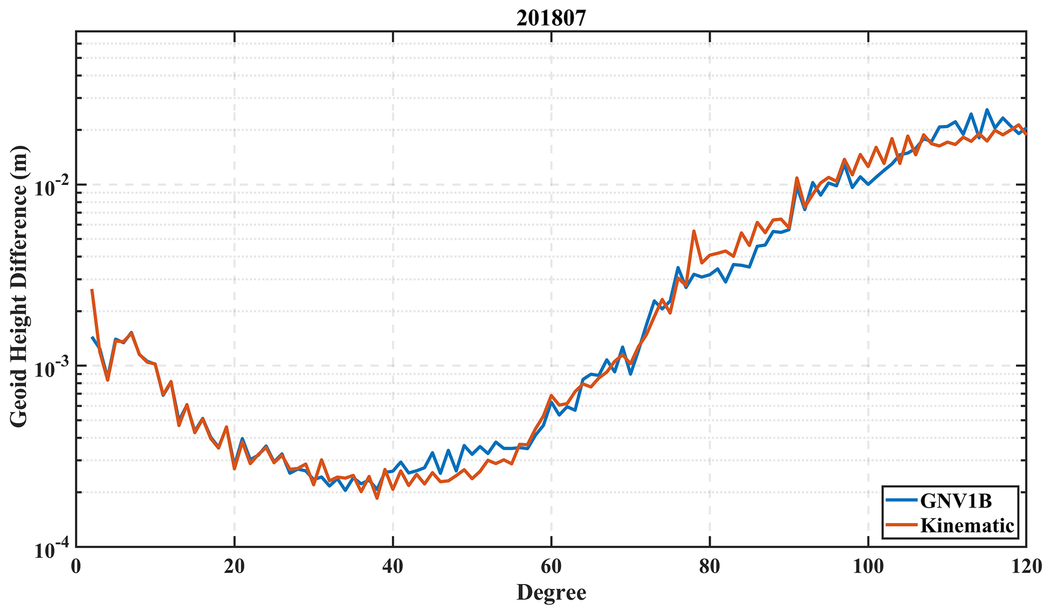
Figure 1 Geoid height difference computed by different orbit products. The blue curve is computed from the reduced dynamic orbit derived from GNV1B and the red curve is computed from the kinematic orbit.

2.2 Renewing of the HUST-GRACE2024 data pre-processing strategy

During temporal gravity field determination, pre-processing of observation data plays an extremely important role in excluding outliers from the final products used in the recovery process. Generally, the data pre-processing procedure includes (1) filling data gaps using an interpolation value and (2) excluding large outliers due to satellite onboard events. For the first aspect, we fill the data gaps in ACC1B and SCA1B using interpolation values, following the method mentioned in the GRACE L1B user handbook (Case et al., 2010). As for the second aspect, we not only exclude the outliers by the data flags but also reject the degraded data, which is associated with satellite onboard events according to the sequence of events (SOE) files. Regarding outliers in the observation data used during temporal gravity field determination, most processing centers exclude these based on the residual value (reference value minus observation data), which is based on the observation instrument data themselves. However, in HUST-Grace2024, we make use of multi-observation data to determine outliers based on cross-validation.

There are several kinds of satellite onboard events, including center of mass (CoM) calibration maneuvers, satellite battery management maneuvers, satellite swap position maneuvers, and orbital maneuvers. Some events, such as the CoM calibration maneuvers, can be found in the SOE file, which will be updated if necessary. For these events found in the SOE file, we add an additional flag to the final pre-processed products, which will not be used in the following gravity field recovery chains. For instance, the accelerometer data are tagged during the CoM calibration maneuvers and the corresponding orbital observation is discarded from the scale factor determination, ultimately maintaining a stable monthly scale factor. However, other events, such as satellite battery management or satellite swap maneuvers, are not recorded in the SOE file, which may also affect the observation quality and contaminate the final gravity solution. Therefore, it is necessary to determine these events according to the special patterns in the observation data.

To determine the events not recorded in the SOE file, a line-of-sight (LOS) Euler angle variation between satellite-based SCA1B and GNV1B data has been developed. Based on this method, satellite swap maneuvers and their related events can be detected. The core of the method is to find the LOS Euler angle variation. The calculation works as follows: firstly, let us denote the rotation matrix from the inertial reference frame (IRF) to the K-band frame (KF) as ${\mathbf{R}}_{\mathrm{IRF}}^{{\mathrm{KF}}_j}$, the matrix from the IRF to the LOS as ${\mathbf{R}}_{\mathrm{IRF}}^{{\mathrm{LOS}}_J}$, and the matrix from the IRF to the science reference frame (SRF) as ${\mathbf{R}}_{\mathrm{IRF}}^{{\mathrm{SRF}}_j}$. The matrixes can be estimated as follows:

$$\begin{array}{}\text{(1)}& {\displaystyle }\begin{array}{rl}& {\mathbf{R}}_{\mathrm{IRF}}^{{\mathrm{SRF}}_j}=\left[\begin{array}{l}{x}_{{\mathrm{SRF}}_j}^T\\ y_{{\mathrm{SRF}}_j}^T\\ z_{{\mathrm{SRF}}_j}^T\end{array}\right]\\ & =\left[\begin{array}{ccc}{q}_{\mathrm{0}}^{\mathrm{2}}+q_{\mathrm{1}}^{\mathrm{2}}-q_{\mathrm{2}}^{\mathrm{2}}-q_{\mathrm{3}}^{\mathrm{2}}& \mathrm{2}\cdot \left(q_{\mathrm{1}}\cdot q_{\mathrm{2}}+q_{\mathrm{0}}\cdot q_{\mathrm{3}}\right)& \mathrm{2}\cdot \left(q_{\mathrm{1}}\cdot q_{\mathrm{3}}-q_{\mathrm{0}}\cdot q_{\mathrm{2}}\right)\\ \mathrm{2}\cdot \left(q_{\mathrm{1}}\cdot q_{\mathrm{2}}-q_{\mathrm{0}}\cdot q_{\mathrm{3}}\right)& q_{\mathrm{0}}^{\mathrm{2}}-q_{\mathrm{1}}^{\mathrm{2}}+q_{\mathrm{2}}^{\mathrm{2}}-q_{\mathrm{3}}^{\mathrm{2}}& \mathrm{2}\cdot \left(q_{\mathrm{2}}\cdot q_{\mathrm{3}}+q_{\mathrm{0}}\cdot q_{\mathrm{1}}\right)\\ \mathrm{2}\cdot \left(q_{\mathrm{1}}\cdot q_{\mathrm{3}}+q_{\mathrm{0}}\cdot q_{\mathrm{2}}\right)& \mathrm{2}\cdot \left(q_{\mathrm{2}}\cdot q_{\mathrm{3}}-q_{\mathrm{0}}\cdot q_{\mathrm{1}}\right)& q_{\mathrm{0}}^{\mathrm{2}}-q_{\mathrm{1}}^{\mathrm{2}}-q_{\mathrm{2}}^{\mathrm{2}}+q_{\mathrm{3}}^{\mathrm{2}}\end{array}\right],\end{array}\text{(2)}& {\displaystyle }\begin{array}{rl}& {\mathbf{R}}_{\mathrm{IRF}}^{{\mathrm{KF}}_j}=\left[\begin{array}{l}{x}_{{\mathrm{KF}}_j}^T\\ y_{{\mathrm{KF}}_j}^T\\ z_{{\mathrm{KF}}_j}^T\end{array}\right]\\ & =\left[\begin{array}{l}{\left({\mathbf{R}}_{\mathrm{IRF}}^{{\mathrm{SRF}}_j}\right)}^T{\left(\frac{\mathrm{phc}}{\left|\mathrm{phc}\right|}\right)}^T{\widehat{\mathit{e}}}_{\mathrm{IRF}}^{\mathrm{SRF}}\\ {\left(z_{{\mathrm{KF}}_j}\times x_{{\mathrm{KF}}_j}\right)}^T\\ {\left(\left(\left(\frac{\mathrm{phc}}{\left|\mathrm{phc}\right|}\right)\left({\mathbf{R}}_{\mathrm{IRF}}^{{\mathrm{SRF}}_j}\right){\widehat{\mathit{e}}}_{\mathrm{IRF}}^{\mathrm{SRF}}\right)\times y_{{\mathrm{SRF}}_j}\right)}^T\end{array}\right],\end{array}\text{(3)}& {\displaystyle }{\mathbf{R}}_{\mathrm{IRF}}^{{\mathrm{LOS}}_j}=\left[\begin{array}{l}{x}_{{\mathrm{LOS}}_j}^T\\ y_{{\mathrm{LOS}}_j}^T\\ z_{{\mathrm{LOS}}_j}^T\end{array}\right]=\left[\begin{array}{l}{\left(\frac{{\mathit{r}}_i-{\mathit{r}}_j}{\left|{\mathit{r}}_i-{\mathit{r}}_j\right|}\right)}^T\\ {\left(\left(\frac{{\mathit{r}}_i-{\mathit{r}}_j}{\left|{\mathit{r}}_i-{\mathit{r}}_j\right|}\right)\times \frac{{\mathit{r}}_i}{\left|{\mathit{r}}_i\right|}\right)}^T\\ {\left(x_{{\mathrm{LOS}}_j}\times y_{{\mathrm{LOS}}_j}\right)}^T\end{array}\right],\end{array}$$

where r_j or r_i denotes the satellite baseline vector (i≠j); phc denotes the phase center, which can be obtained from VKB1B; $q_{\mathrm{0}},q_{\mathrm{1}},q_{\mathrm{2}}$, and q₃ are the quaternion numbers, which can be derived from SCA1B; ${\widehat{\mathit{e}}}_{\mathrm{IRF}}^{\mathrm{SRF}}$ is the unit vector from the IRF to the SRF; and index j is the satellite ID.

Secondly, substitute Eqs. (2) and (3) into Eq. (4) as follows:

$$\begin{array}{}\text{(4)}& {\mathbf{R}}_{\mathrm{KF}}^{\mathrm{LOS}}={\mathbf{R}}_{\mathrm{IRF}}^{\mathrm{LOS}}{\left({\mathbf{R}}_{\mathrm{IRF}}^{\mathrm{KF}}\right)}^T,\end{array}$$

where j is omitted for better demonstration. Note that ${\mathbf{R}}_{\mathrm{KF}}^{\mathrm{LOS}}$ is a rotation matrix for transforming from the KF to the LOS. Thus, the rotation matrix can be divided into three independent directions as follows:

$$\begin{array}{}\text{(5)}& {\mathbf{R}}_{\mathrm{KF}}^{\mathrm{LOS}}=R_{\mathrm{1}}\left(\mathit{\varphi }\right)R_{\mathrm{2}}\left(\mathit{\theta }\right)R_{\mathrm{3}}\left(\mathit{\psi }\right),\end{array}$$

where ϕ, θ, and ψ are the Euler pointing angles roll, pitch, and yaw, respectively.

Based on the aforementioned method, the Euler angle variations for 6 September 2011 and 4 January 2013 are shown in Fig. 2. It can be clearly seen that there is a huge data gap in the KBR range-rate data lasting from 14:00:00 to 14:45:00 UTC + 0. At the same time, there is a notable oscillation in the yaw angle variation data. Thus, there are some connections between range-rate data loss and yaw angle change. When the yaw angle exceeds a certain threshold, e.g., 50 mrad, there is a data gap in the range-rate data.

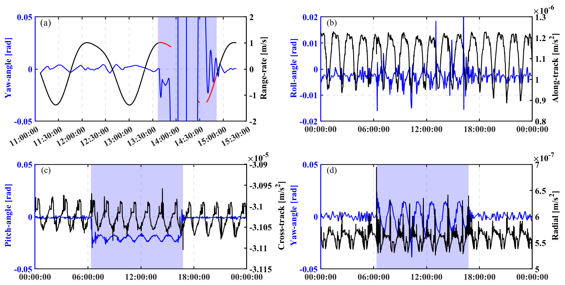
Figure 2 (a) Time series of GRACE-A yaw pointing angle variations (blue lines) during yaw-turn maneuvers on 6 September 2011. The KBR range rates are plotted as black lines, and the screened data are shown in red. The KBR observations for the time period highlighted in light blue are not used in the following temporal gravity field recovery process. (b–d) Time series of Euler pointing angle variations (blue lines) during CoM calibration maneuvers on 4 January 2013. The ACC observations in along-track, cross-track, and radial directions for GRACE-A are also shown as black lines.

Comparing the Euler angles shown in Fig. 2a, we set 50 mrad as the threshold for yaw angle variation and 100 s as the margin interval. Therefore, when the Euler angles exceed the threshold, the corresponding range rates in the margin interval will be excluded from the following gravity field recovery process. To illustrate the necessity of excluding these observations, as shown in Fig. 3, the geoid height variance per degree is also computed via different pre-processing strategies (including original processing and updated processing strategies). In January 2005 there were also some yaw-turn maneuvers, as shown in Fig. 2a, which degraded the quality of the KBR range-rate data. In the updated processing strategy, we exclude the KBR range-rate data in the corresponding time based on the aforementioned method of outlier detection. Compared to the original processing strategy, the updated pre-processing strategy has a relatively smaller geoid height difference per degree from degree 35 to degree 90, with a reduction of about 13 % at most. This clearly illustrates the benefit of updating the pre-processing strategy.

Figure 3 The geoid height variance of gravity fields in January 2005 computed by the original processing strategy (blue lines) and the updated processing strategy (red lines).

During the CoM calibration maneuvers, as shown in Fig. 2b to d, the pointing angle, especially the yaw angle, changes in a sine-like pattern with an amplitude of about 20 mrad. In this study, according to the SOE file, the CoM calibration maneuvers are executed at the same time. This is reasonable since the CoM offset will be set to constant during calibration maneuvers, which last about 180 s. During this time, the linear acceleration in three directions will suffer from a regular square wave variation without additional thruster firing. Actually, only a start-time tag and a finish-time tag are recorded during CoM calibration. Based on this method, in the HUST-Grace2024 gravity field series, the SOE file is used for picking out the calibration campaign time tag and the Euler angle variation is also computed. The degraded data in a specific arc are excluded during monthly scale factor estimation and gravity field determination.

2.3 Hybrid data-weighting method

In this section, the second improvement of the processing chain in HUST-Grace2024 is discussed, which mainly focuses on developing a hybrid data-weighting method for gravity field determination. Except for the systematic errors, which can be physically corrected beforehand, there is still some random noise in the observations. Therefore, it is necessary to construct a proper hybrid weighting method that can comprehensively process the systematic errors and the random noise.

The estimation of geopotential coefficients can be described as follows:

$$\begin{array}{}\text{(6)}& \begin{array}{rl}x& =(A_{\mathrm{orbit}}^T{P}_{\mathrm{orbit}}{A}_{\mathrm{orbit}}+A_{\mathrm{kbr}}^T{P}_{\mathrm{kbr}}{A}_{\mathrm{kbr}}{)}^{-\mathrm{1}}\\ & (A_{\mathrm{orbit}}^T{P}_{\mathrm{orbit}}{l}_{\mathrm{orbit}}+A_{\mathrm{kbr}}^T{P}_{\mathrm{kbr}}{l}_{\mathrm{kbr}}),\end{array}\end{array}$$

where x, A_orbit, P_orbit, and l_orbit denote the unknown geopotential coefficient, the design matrix for the satellite orbit, the stochastic model for the orbit, and the orbit residual vector computed by integration of the orbit minus the observation orbit derived from L1B data, respectively. A_kbr, P_kbr, and l_kbr denote the design matrix, the stochastic model, and the residual vector for the KBR observation data, respectively.

For P_kbr, the stochastic model is constructed using post-fit range-rate residuals. As shown in Fig. 4a, the KBR range-rate pre-fit residuals suffer from low-frequency noise (< 1 mHz) associated with the satellite orbit, where its relationship can be described by the Hill equation (Colombo, 1984), and high-frequency random noise (> 10 mHz).

Figure 4 (a) Power spectral density (PSD) of 1-month GRACE KBR range rates in January 2005. The red line is computed by KBR pre-fit residuals, while the blue line is computed by KBR post-fit residuals. (b) Geoid height difference of gravity fields in January 2005 computed by different low-frequency noise processing strategies including KBR data via COV (red line), KBR (green line), and KBR+COV (blue line), where COV denotes a covariance stochastic model matrix, KBR denotes range-rate empirical parameters, and COV+KBR denotes a hybrid pre-processing strategy including COV and KBR.

For the low-frequency noise in range-rate data, some range-rate empirical parameters are commonly used in low-frequency noise reduction (Zhou et al., 2018; Nie et al., 2021). However, the high-frequency random noise cannot be reduced as much as the low-frequency noise. As shown in Fig. 4a, it is noticeable that some gravity signals can be derived from KBR pre-fit residuals, while the temporal signals can hardly be retrieved from KBR pre-fit residuals over 10 mHz. In order to retrieve as many gravity signals as possible, the correlations among range-rate observations must be taken into consideration via a stochastic model.

Based on the method proposed by Ditmar (2006), the covariance matrix P_kbr is constructed by the auto-covariance vector, which originates from the post-fit residuals of KBR observations. The steps of constructing a covariance matrix can be summarized as follows:

• a.

  computation of the auto-covariance vector for post-fit range-rate residual series using

  $$\begin{array}{}\text{(7)}& a_k={\displaystyle \frac{\mathrm{1}}{N_k}}\sum _i{s}_i{s}_{i+k}(\mathrm{0}\le i\le n),\end{array}$$

  where a_k denotes the kth auto-covariance vector element, N_k denotes the pairs of post-fit residual elements used for the auto-covariance element estimation, and i denotes the lag between different epochs in the residual series. It should be kept in mind that k must be in the interval (0, n), where n is the total number of residual series. After calculating the auto-covariance vector,

• b.

  the Toeplitz covariance matrix is then constructed as follows:

  $$\begin{array}{}\text{(8)}& \left(\left.\begin{array}{cccc}{a}_{\mathrm{0}}& \mathrm{\cdots }& a_{n-\mathrm{1}}& a_n\\ \mathrm{⋮}& a_{\mathrm{0}}& \mathrm{\cdots }& a_{n-\mathrm{1}}\\ a_{n-\mathrm{1}}& \mathrm{\cdots }& \mathrm{\ddots }& \mathrm{⋮}\\ a_n& a_{n-\mathrm{1}}& \mathrm{\cdots }& a_{\mathrm{0}}\end{array}\right).\right.\end{array}$$

Following the aforementioned methods, we design an experiment to investigate the effect of different strategies for KBR observations in real GRACE gravity field determination, as shown in Fig. 4b. During the experiment, the strategies using the range-rate empirical parameters (KBR in Fig. 4b), the covariance matrix (COV in Fig. 4b), and the hybrid data-weighting approach COV+KBR are applied. It is obvious that all strategies have almost the same long-wavelength gravity-signal-capture ability, while the estimation via the hybrid approach COV+KBR presents the smallest geoid height variance. There are still some results that should be highlighted: (1) the COV approach is noticeably different from the KBR approach, especially for estimations above degree 20. (2) The result of the hybrid approach is slightly better than that of the COV approach between degrees 25 and 50. The results in Fig. 4b provide us with an insight into the characteristics of the different KBR data processing strategies.

For the first part of the results, the relationship between the COV method and the KBR method, which can be combined by least squares collocation, has been described by Nie et al. (2022). However, the results in Fig. 4b demonstrate that there is still some difference between the COV method and the KBR method for real data processing. To qualify the difference, the gravity field determination Eq. (6) can be rewritten as follows:

$$\begin{array}{}\text{(9)}& \begin{array}{rl}x& =(A_{\mathrm{orbit}}^T{P}_{\mathrm{orbit}}{A}_{\mathrm{orbit}}+A_{\mathrm{kbr}}^T{F}^T{\mathbf{Q}}_{\mathrm{kbr}}F{A}_{\mathrm{kbr}}{)}^{-\mathrm{1}}\\ & (A_{\mathrm{orbit}}^T{P}_{\mathrm{orbit}}{l}_{\mathrm{orbit}}+A_{\mathrm{kbr}}^T{F}^T{\mathbf{Q}}_{\mathrm{kbr}}F{l}_{\mathrm{kbr}}),\end{array}\end{array}$$

where F denotes a linear operator, and Q_kbr implies the stochastic model matrix. If the result of gravity field determination remains the same, the COV and KBR method must meet the requirements of Eq. (10):

$$\begin{array}{}\text{(10)}& P_{\mathrm{kbr}}=F^T{\mathbf{Q}}_{\mathrm{kbr}}F.\end{array}$$

However, Eq. (10) can hardly be achieved in real gravity field determination due to the operator characteristic of F. Different from the KBR method, the COV method is constructed based on the correlation of range-rate observations, including all signals in the target frequency band. Thus, the COV method results in better gravity field estimations than the KBR method.

In conclusion, the COV method mainly attenuates the effect of random noise in range-rate observations during gravity field determination, while the KBR method mainly attenuates the systematic effect from the orbit. Therefore, our hybrid data-weighting method combining COV with KBR can achieve a better result than the individual methods.

2.4 Strategy for accelerometer calibration

Generally, the raw ACC1B measurement data are degraded by unknown scale factors, time-varying biases, and other unknown noise; therefore, the data need to be calibrated using Eq. (11) before the gravity field determination:

$$\begin{array}{}\text{(11)}& {\displaystyle }{a}_{\mathrm{cal}}=R\cdot (\mathbf{S}\cdot a_{\mathrm{obs}}+b_{\mathrm{bias}}),\text{(12)}& {\displaystyle }\mathbf{S}=\left[\begin{array}{ccc}{s}_x& \mathit{\alpha }+\mathit{\zeta }& \mathit{\beta }-\mathit{\epsilon }\\ \mathit{\alpha }-\mathit{\zeta }& s_y& \mathit{\gamma }+\mathit{\delta }\\ \mathit{\beta }+\mathit{\epsilon }& \mathit{\gamma }-\mathit{\delta }& s_z\end{array}\right],\end{array}$$

where a_obs denotes the non-gravitational forces observed by the onboard accelerometer, S denotes the scale factor matrix, b_bias implies the bias vector for calibration, R implies the rotation matrix transforming the accelerometer observations from the SRF to the IRF, and a_cal denotes the calibrated accelerometer measurements. It should be noted that there are three parts to the scale factor matrix S: (1) main diagonal elements consisting of s_x, s_y, and s_z; (2) shear elements consisting of α, β, and γ; and (3) rotational elements including ζ, ε, and δ.

As shown in Table 1, the following accelerometer calibration parameters for HUST-Grace2024 are estimated: (1) a monthly fully populated scale factor matrix including main diagonal and off-diagonal elements and (2) a 6 h bias vector including constant first-time-derivate and second-time-derivate bias elements for along-track, cross-track, and radial directions. Based on the calibration in Eq. (11), we estimated the scale factor matrix as shown in Fig. 5. The scale factor variation is similar for both GRACE-A and GRACE-B, and thus only the parameters for GRACE-A are plotted in this figure.

The main diagonal element in the cross-track direction is not estimated to be as stable as those in the other two directions, a fact which derives from the limited sense of the accelerometer in the cross-track direction. Moreover, for the radial axis, the main diagonal scale factors fluctuated more violently from 2002 to 2006 and from 2012 to 2017 than from 2007 to 2011. This violent fluctuation may be associated with a time period of solar activity, which is supported by Koch et al. (2019). When the solar activity is serene, the scale factor in the radial direction can be estimated stably during the period from 2006 to 2010, while it cannot be estimated as stably from 2012 to 2017. A clearly reduced along-track scale factor can be seen after 2011 due to the switched-off thermal control for GRACE-A. Meanwhile, the scale factor in the radial direction becomes more and more scattered as the GRACE mission moves on. The results indicate that the scale factor itself has a clearly reduced behavior, which is consistent with the results shown by Klinger and Mayer-Gürr (2016). When comparing to the main diagonal estimations derived from GRACE, those derived from GRACE-FO are notably scattered, especially for the along-track estimations. The scattered estimations are mainly due to the relatively degraded performance of GRACE-FO onboard accelerometers.

As for the rotation and shear elements, these are not presented as constants but rather vary with very similar patterns, which indicates that the misalignment between the SRF and the accelerometer frame (AF) has a close connection with the non-orthogonality of the three AF axes. In addition, there is a generally comparable performance between GRACE and GRACE-FO estimations, demonstrating the comparable alignment accuracy for the SRF and the AF as well as the orthogonality of the three AF axes.

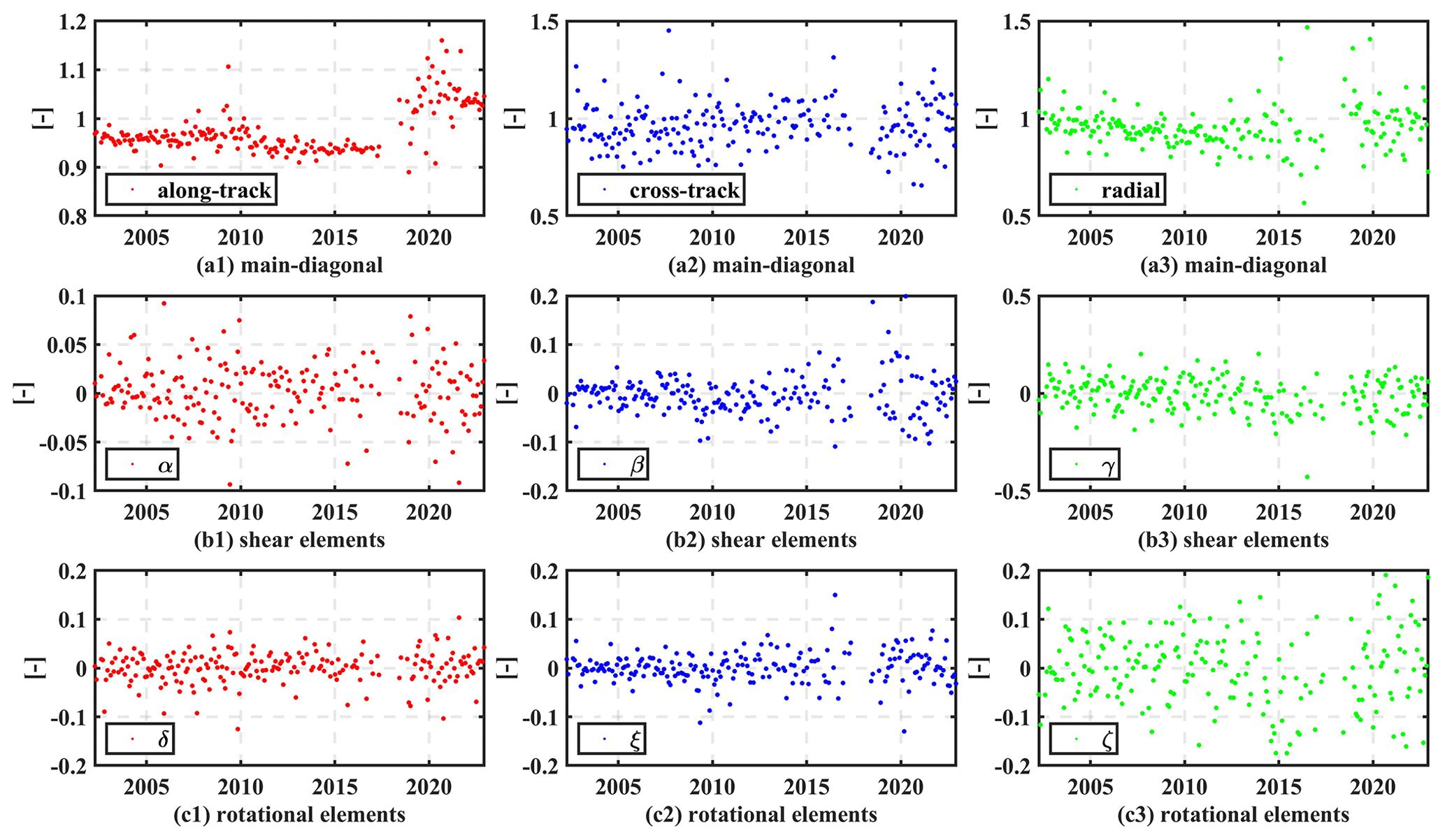
Figure 5 Full calibration scale factor elements for GRACE-A in monthly resolution. (a1–a3) Main diagonal elements in along-track (red), cross-track (blue), and radial (green) directions. (b1–b3) Shear element variation of α (red), β (blue), and γ (green). (c1–c3) Rotational element variation of δ (red), ξ (blue), and ζ (green).

Table 2 Mean value and standard deviation of accelerometer scale factors for GRACE-A and GRACE-B during the period from April 2002 to June 2017. The corresponding prior values from TN02 are also listed (Bettadpur, 2009).

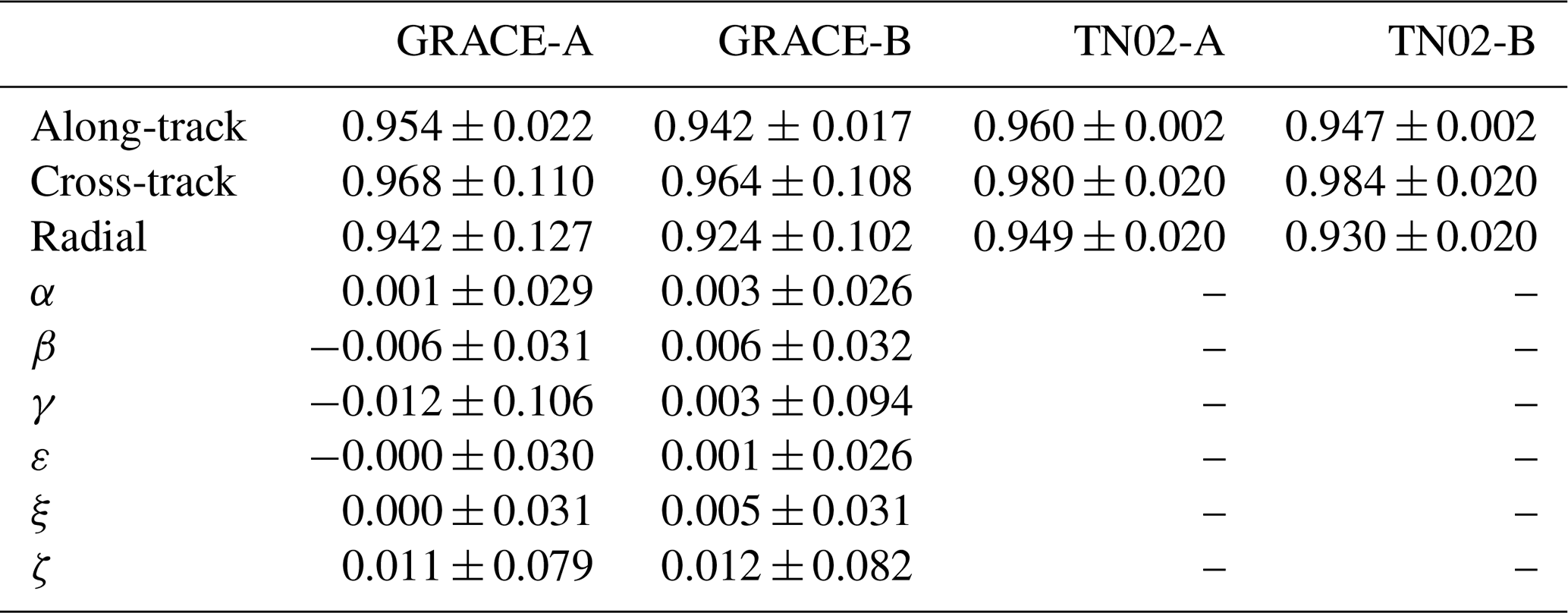
For a general comparison of the scale factors during the whole GRACE lifetime, we compute the corresponding mean values and standard deviations for GRACE-A and GRACE-B. Meanwhile, the prior values of the main diagonal elements from TN02 are also listed in Table 2. The mean values of the scale factor in along-track, cross-track, and radial directions estimated for HUST-Grace2024 are close to the corresponding prior values derived from TN02, which demonstrates the stability of our accelerometer parameterization strategy. Note that although these mean values for HUST-Grace2024 have a close connection with TN02 (although they are not exactly the same), the scale factors still need to be estimated again along with the geopotential coefficients to avoid potential temporal signal attenuation (Zhou et al., 2019). Except for the main diagonal elements, we also compute the mean values of rotational and shear elements. According to Table 2, the mean values are quite small (not zero), while the relevant standard deviations are still noteworthy when compared to those for the main diagonal. This indicates the necessity of estimating rotational elements and shear elements, which supports the concept of misalignment between the SRF and the AF and the non-orthogonality of the three AF axes.

Overall, our hybrid processing chain contribution to HUST-Grace2024 can be summarized as follows: (1) we update the observations, background force models, and key parameter estimation strategies for the whole observation period of the GRACE and GRACE-FO missions. Meanwhile, based on the fully populated scale factor matrix, we obtain relatively stable accelerometer scale factors. Compared with GRACE estimations, the accelerometer scale factors of the GRACE-FO mission fluctuate more widely. (2) We make full use of the inter-satellite pointing angles to detect outliers in accelerometer and range-rate data, which differs from previous studies and the outlier detection methods of other processing centers. In addition, we perform a quantitative analysis related to the impacts of our outlier detection method on temporal gravity field determination, which can also be an important instruction to quantitatively analyze the effect of satellite onboard events in the data processing chain. (3) We perform a comprehensive quantitative analysis of different weighting approaches for frequency-dependent noise in range rates and further analyze their impacts on temporal gravity field determination.

3 GRACE results

3.1 The HUST-Grace2024 model

Based on the updated processing chain, a new temporal gravity field series covering the entire lifetime of the GRACE and GRACE-FO science missions from 2002 to 2022 named HUST-Grace2024 has been developed. To evaluate the performance of HUST-Grace2024, we perform a comprehensive comparison with the latest official gravity field solutions, including those from the CSR, the GFZ, and the JPL, in both the spectral and the spatial domains. The time span for the gravity field solution assessment is selected as 2005 to 2016 for GRACE solutions and 2018 to 2022 for GRACE-FO solutions.

3.1.1 Analysis in the spectral domain

A commonly used parameter to quantify the quality of GRACE solutions in the spectral domain is the geoid height variance compared to a static gravity field. In this section, the static field EIGEN-6C4 is used as the base gravity field. The geoid height difference is dominated by the temporal gravity signal for low-degree geopotential coefficients, while it is dominated by the mismodeling gravity signal for high degrees. Therefore, the smaller geoid height variance per degree at high degrees over 40 can be used as a criterion for evaluating the GRACE solutions in the spectral domain.

As shown in Fig. 6, the geoid height difference per degree of HUST-Grace2024 is compared with three official solutions, including CSR RL06, GFZ RL06, and JPL RL06 (RL06.1 for GRACE-FO solutions). Generally, HUST-Grace2024 has almost the same or slightly better ability to retain long-wavelength signals in the temporal gravity field, while there is a noticeable noise reduction of geopotential coefficients at high degrees. As shown in Fig. 6a to f, the geoid height difference per degree of HUST-Grace2024 in particular is smaller than the values of the official solutions from degree 40 to degree 80, indicating a better performance of the HUST-Grace2024 model in capturing high-frequency mass transportation.

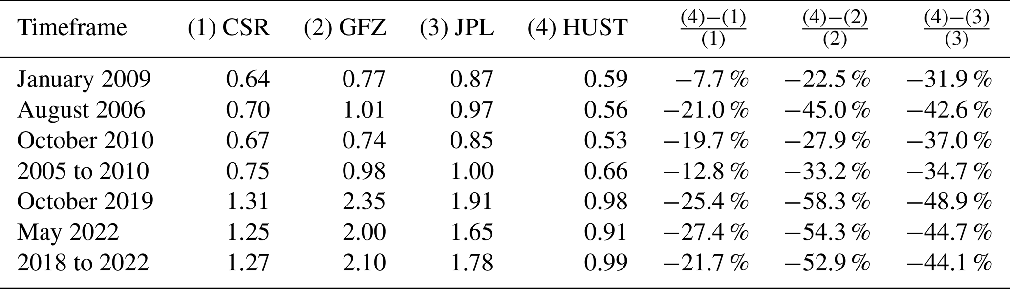
For a better comparison of the spectral characteristics for HUST-Grace2024, as listed in Table 4, we also computed the cumulative geoid height difference for HUST-Grace2024 and three official solutions. During the period from 2005 to 2010, the average cumulative difference was 0.75, 0.98, 1.00, and 0.66 cm for CSR RL06, GFZ RL06, JPL RL06, and HUST-Grace2024, respectively, indicating an average cumulative geoid height difference reduction of −12.8 %, −33.2 %, and −34.7 % for the HUST-Grace2024 model when compared to the official solutions, respectively. Especially in August 2006, the reduction for HUST-Grace2024 reached 45.0 % and 42.6 % when compared to GFZ RL06 and JPL RL06, respectively. As for the GRACE-FO mission period, the noise reductions for HUST-Grace2024 become even more notable when compared to the official solutions. The results indicate that our hybrid processing strategy is likely more efficient for the GRACE-FO observations. The reduction of the geoid height difference may be contributed to by the degrees up to 40. In order to assess the temporal signal in HUST-Grace2024, we need to perform an analysis in the spatial domain as described in the following section.

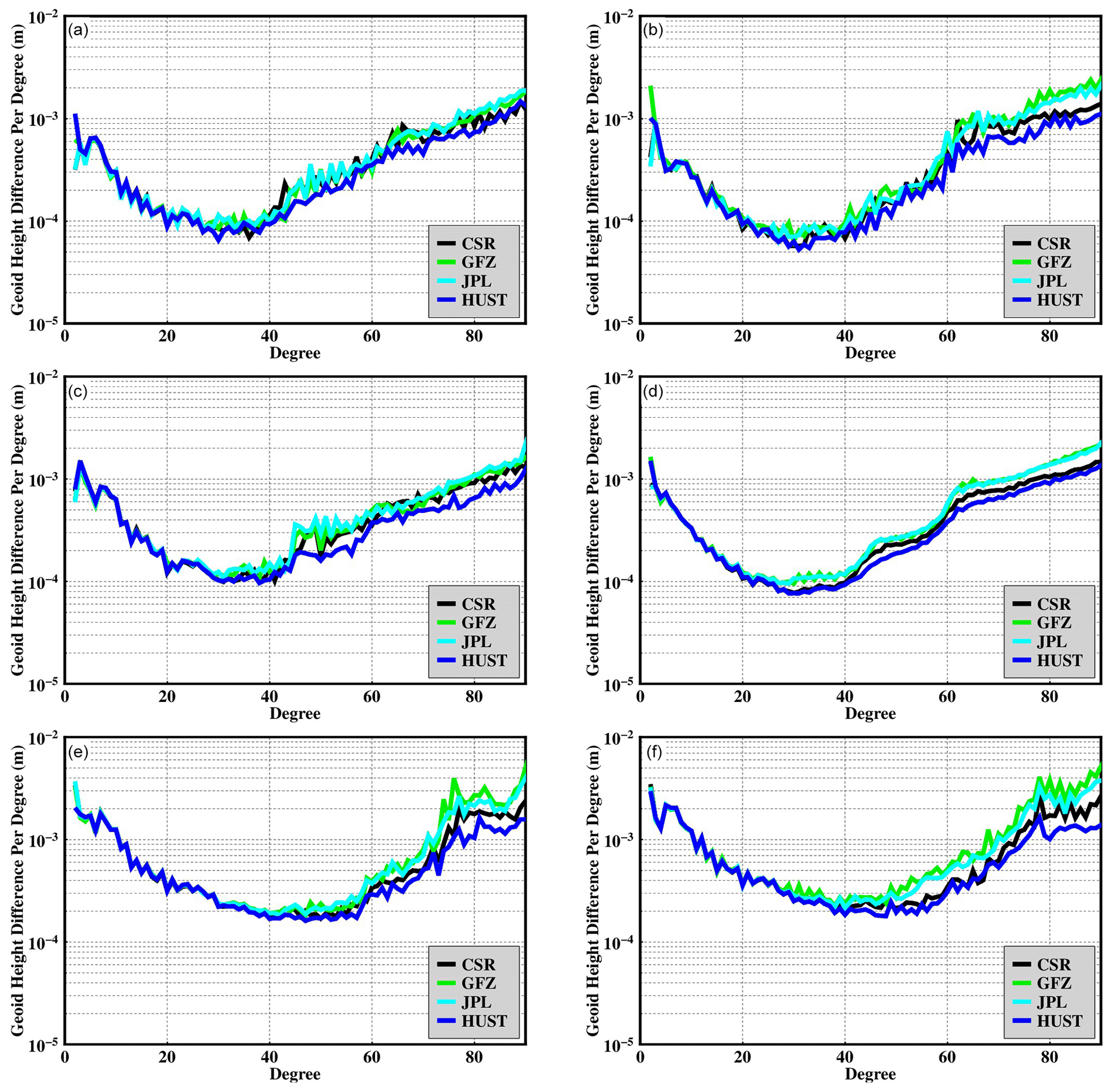
Figure 6 Geoid height difference per degree of temporal gravity model in different months including (a) January 2009, (b) August 2006, (c) October 2010, (d) 2005 to 2010, (e) October 2019, and (f) May 2022.

C₂₀ has the largest magnitude among the geopotential coefficients and a close connection to the Earth's geodynamic process and large-scale mass transportation (e.g., Cheng and Ries, 2023; Landerer et al., 2020; Velicogna et al., 2020). It is very important to obtain an accurate C₂₀ estimation during temporal gravity field determination. As shown in Fig. 2, the non-gravitational signal observed by the accelerometer exhibits periodic variation, such as 1-CPR and 2-CPR later on. The non-gravitational feature can be captured by the resonance orders of the geopotential coefficient. Satellite laser ranging (SLR) tracking consists of several geodetic satellites such as Starlette, Stella, and Ajisai, which are operated at different altitudes and experience different “lump effects” of geopotential coefficients. Thanks to the characteristics of SLR, zonal coefficients derived from SLR are more reliable than those derived from GRACE (Cheng and Ries, 2017, 2023). Therefore, we compare the geopotential coefficients from GRACE solutions with those derived from SLR, thereby qualifying the accelerometer calibration method indirectly. Besides this, C₂₀ and C₃₀ are degraded and corrupted by the thermal noise in the accelerometer and a 161 d periodic signal, and the values need to be replaced by SLR, especially after the thermal control was switched off in 2011 during the GRACE science mission.

As shown in Fig. 7, generally, the variation of C₂₀ derived from HUST matches that derived from SLR well. The correlation coefficient for C₂₀ with SLR is also computed, as listed in Table 3. It is clearly implied that the correlation coefficient between HUST and SLR is 0.86, and between the other science data systems (SDSs) and SLR it is 0.86, 0.80, and 0.75 for CSR, GFZ, and JPL, respectively. The correlation coefficients also demonstrate that our new calibration method ensures accurate C₂₀ estimations for HUST-Grace2024.

Apart from the C₂₀ results, the other low-degree coefficients derived from HUST also show good agreement with those derived from the other SDSs. The C₃₀ estimations for the gravity field official solution centers, including HUST, are slightly overestimated compared to those derived from SLR. The overestimated C₃₀ is related to the satellite internal temperature stability and the Sun vs. eclipse exposure changes, which it is advisable to replace by the SLR estimation (Kvas et al., 2019a). As for C₂₁ and S₂₁, the results of HUST are consistent with those of CSR and JPL. In addition, for C₂₁, S₂₁, C₂₂, and S₂₂, general consistency is also observed between the GRACE and GRACE-FO estimations.

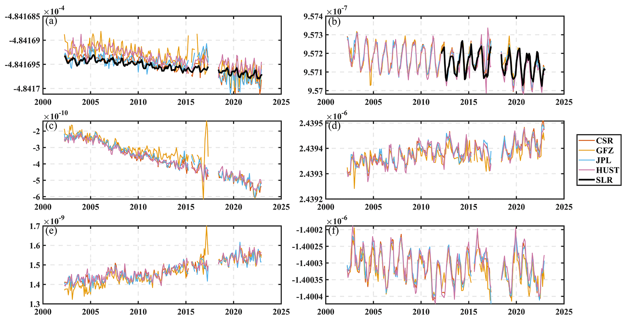
Figure 7 Geopotential coefficients derived from SLR, CSR, GFZ, JPL, and HUST. The geopotential coefficients include C₂₀ (a), C₃₀ (b), C₂₁ (c), C₂₂ (d), S₂₁ (e), and S₂₂ (f) during the period from 2002 to 2022. Note that the SLR curve is only shown in (a) and (b).

Table 3 Correlation coefficient along with SLR computed by C₂₀ derived from different science data systems (SDSs). Note that the result of SLR is derived from the TN-14 document (Loomis et al., 2020).

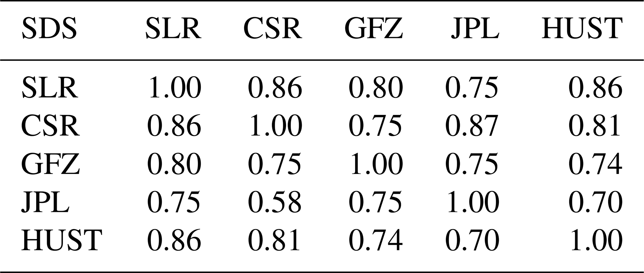
Table 4 Cumulative geoid height differences (in centimeters) of CSR, GFZ, JPL, and the HUST-Grace2024 model. All models are truncated up to degree and order 96.

3.1.2 Analysis in the spatial domain

In order to evaluate the performance of our HUST-Grace2024 model in the spatial domain, the global mass changes are calculated in terms of equivalent water heights (EWHs) with a resolution of 1°, smoothed by a 300 km Gaussian filter and a P3M6 decorrelation filter. Based on the global EWHs, the commonly used spatial criteria are then computed, including annual amplitudes, yearly trends, and root mean square (rms) values of temporal signal residuals. Here, the annual amplitudes and yearly trends are used to assess the performance of retrieving temporal signals, while the rms values are used for the temporal noise evaluation. As shown in Eq. (13), the rms values are calculated on the basis of the terrestrial water storage anomaly (TWSA) residuals, which have removed the yearly trends, semi-annual amplitudes, and annual amplitudes from the original time series:

$$\begin{array}{}\text{(13)}& \begin{array}{rl}\mathrm{rms}& =\mathrm{rms}({\mathrm{TWSA}}_{\mathrm{total}}-{\mathrm{TWSA}}_{\mathrm{trend}}\\ & -{\mathrm{TWSA}}_{\text{annual-amplitude}}-{\mathrm{TWSA}}_{\text{semiannual-amplitude}}).\end{array}\end{array}$$

The global annual amplitudes and yearly trends for different GRACE solutions during the period from 2005 to 2016 are displayed in Fig. 8, while those for the GRACE-FO solution are shown in Fig. 9. The annual amplitude for HUST-Grace2024 exhibits good agreement with the official solutions in the areas of South America, central Africa, and the south of Asia, ensuring the model's ability to capture large-scale mass change over the world. In addition, the rms value for the result without any filter is also plotted as shown in Figs. 10 and 11. In order to mitigate signal leakage from the land into the ocean, we create a 400 km buffer zone from the coastline for the results. The temporal noise in HUST-Grace2024 is significantly smaller than the solutions derived from JPL and GFZ, while it is generally comparable with the CSR result. Indeed, we do not account for the impact of co-seismic and post-seismic changes during the computation of the TWSA residuals. The effects of seismic changes are local and not significant in the TWSA residual rms distribution, which may be beyond the research scope of this paper.

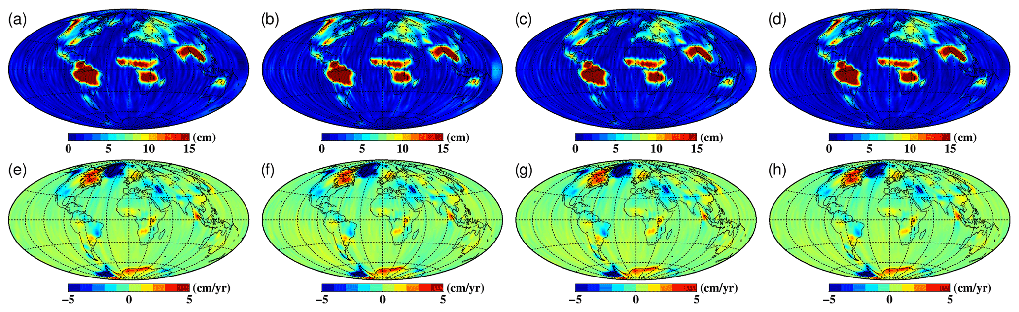
Figure 8 Global annual amplitudes (top row) and yearly trends (bottom row) during the period from 2005 to 2016 as derived from different products including (a, e) CSR RL06, (b, f) GFZ RL06, (c, g) JPL RL06, and (d, h) HUST-Grace2024. Note that all results are smoothed by a 300 km Gaussian filter and P3M6 decorrelation filter.

Figure 9 Same as Fig. 8 but for GRACE-FO solutions during the period from 2018 to 2022.

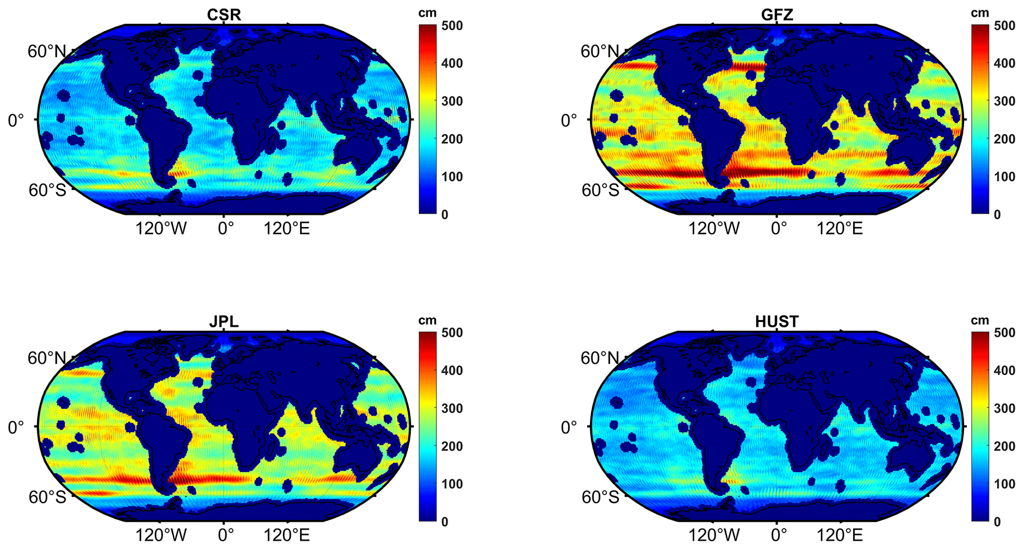
Figure 10 The rms value of the EWH residual, which is computed from the EWHs minus their climatology part (bias, amplitude, and trend) for different GRACE solutions during the period from 2005 to 2016 over the open ocean with a 400 km buffer zone from the coastline. Note that no filter is applied here.

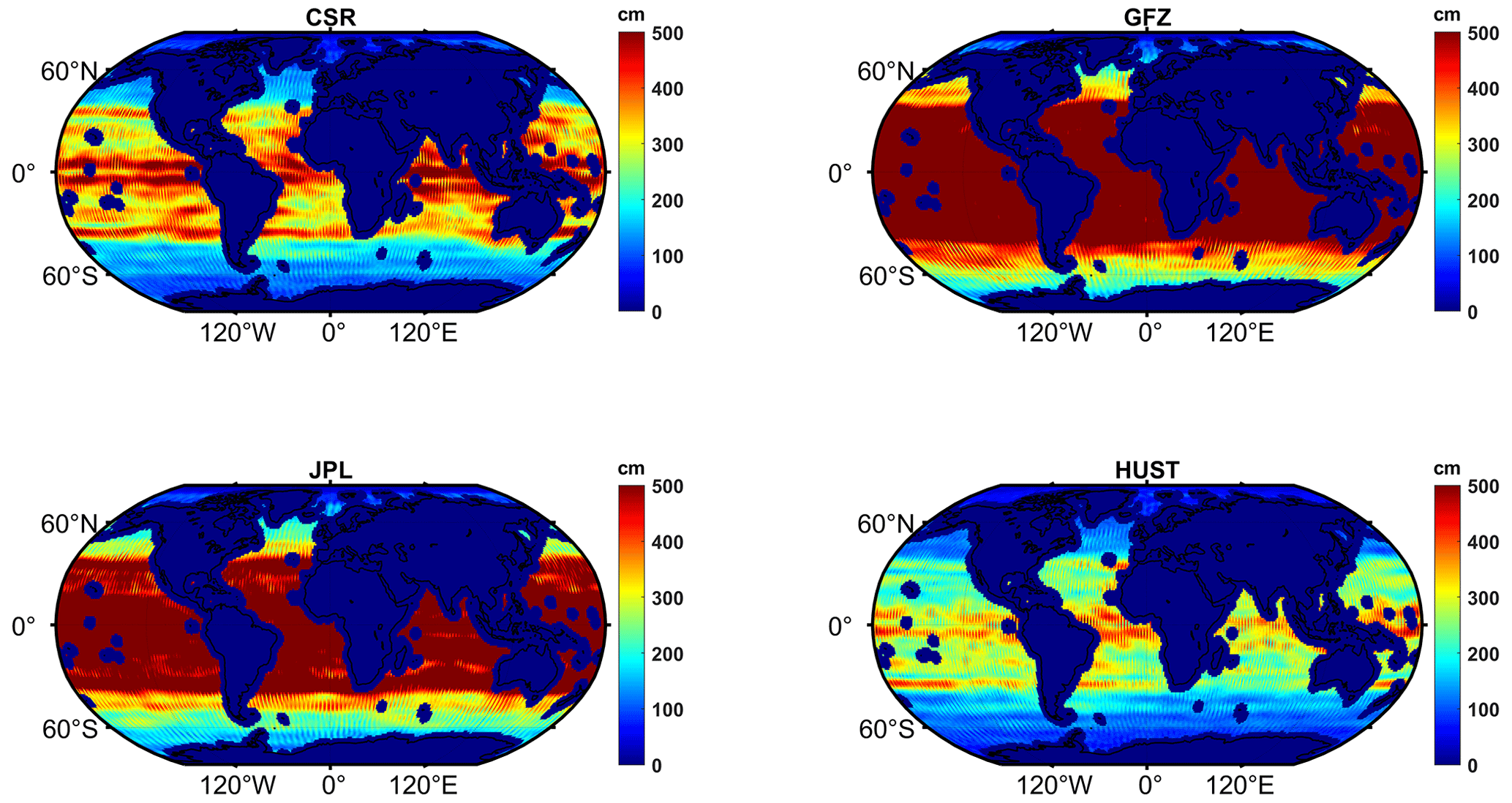
Figure 11 Same as Fig. 10 but for GRACE-FO solutions during the period from 2018 to 2022.

In order to assess the noise level of our HUST-Grace2024 model, we select an open-ocean area as shown in Figs. 10 and 11, which is considered to have the smallest temporal signal remaining and be very suitable for the temporal gravity field assessment in the spatial domain.

The EWH residual is computed from the EWHs (without any filter) minus their climatology part (bias, amplitude, and trend) based on the temporal gravity field derived from CSR RL06, JPL RL06, GFZ RL06, and HUST-Grace2024 during the period from 2005 to 2016. As shown in Fig. 12, in most months from 2005 to 2016, the residuals over a selected open ocean in our model are significantly smaller than those from JPL and GFZ, while being comparable with those from CSR. The rms values of the residuals are 132.3, 228.1, 209.2, and 118.0 cm for CSR RL06, GFZ RL06, JPL RL06, and HUST-Grace2024, respectively. In addition, in our GRACE-FO solution, the residual EWH over a selected open ocean is further reduced when compared to the latest official solution RL06.1. The rms value of the residual is 235.2, 488.6, 390.3, and 177.7 cm for CSR RL06.2, JPL RL06.1, GFZ RL06.1, and HUST-Grace2024, respectively. The GRACE-FO solution indicates that our hybrid processing can significantly reduce the temporal noise over the open ocean when compared to the GRACE solution.

Figure 12 Equivalent water height (EWH) residual over a selected open-ocean series during the period from 2005 to 2016 and 2018 to 2022. The residual is computed from the EWH (without any filter) minus its climatology part (bias, amplitude, and trend).

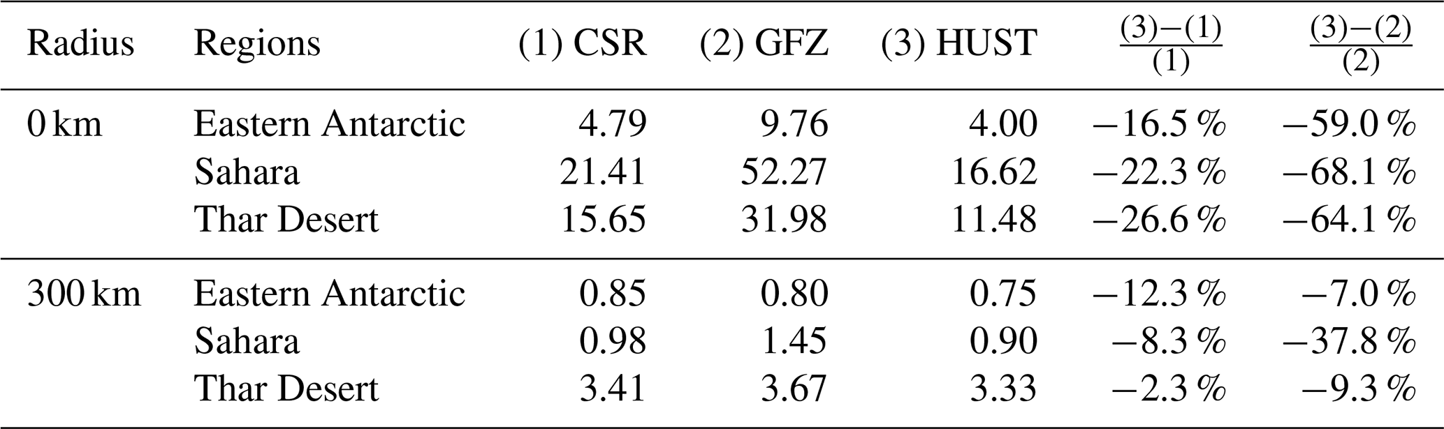
For a more quantitative comparison of the noise level between the HUST product and the latest official GRACE-FO solutions, we calculate the weighted mean of the rms EWH residual over the representative deserts and the east of the Antarctic, which is assumed to have an extremely small remaining temporal signal. Due to the fact that the climatology part (bias, trend, and amplitude) has been removed from the residual result, the residual can be regarded as a mismodeling signal or temporal noise that remained in the model solution. As listed in Table 5, in the Sahara, the residual for our solution is 0.90 cm, but it is 0.98 cm and 1.45 cm for CSR and GFZ, respectively, thus indicating that the noise reduction of our GRACE-FO solution is 8.3 % and 37.8 %, respectively, when compared to the CSR and GFZ solutions. In addition, the noise reductions of our HUST-Grace2024 model become more significant when no filter is applied. For instance, the reductions over the Sahara reach 22.3 % and 68.1 % when compared to the CSR and GFZ solutions, respectively. A similar phenomenon is also observed over the east of the Antarctic and the Thar Desert.

Table 5 Weighted mean EWH residual (in centimeters) over the representative deserts and the east of the Antarctic. Note that results without any filter and with a 300 km Gaussian filter are computed. The locations of the representative assessment areas are listed here as the eastern Antarctic (74–80° S, 60–120° E), the Sahara (28–34° N, 3° W–9° E), and the Thar Desert (23–30° N, 70–75° E).

In order to assess the performance of our model in terms of retaining temporal signal, we compute the annual amplitudes over 48 representative river basins. The locations of these 48 representative river basins are the same as those in Fig. S3 in Zhou et al. (2018). Following Scanlon et al. (2016) and Zhou et al. (2018), the scatters of the annual amplitudes for 48 river basins are plotted for the cross-comparison between different GRACE-FO solutions (Fig. 13). The GRACE-FO solutions included CSR RL06.2, GFZ RL06.1, JPL RL06.1, and HUST-Grace2024. Theoretically, when the slope of the fitted line (the dashed black line in Fig. 13) is closer to 1, the temporal signals derived from different models are more similar. Compared with HUST-Grace2024, the scatters are close to the fitted line, and the slope is 1.00, 1.03, and 1.00 for CSR RL06.1, GFZ RL06.1, and JPL RL06.1, respectively. This demonstrates the generally good agreement between our model and the three official models for retrieving basin-scale temporal signals.

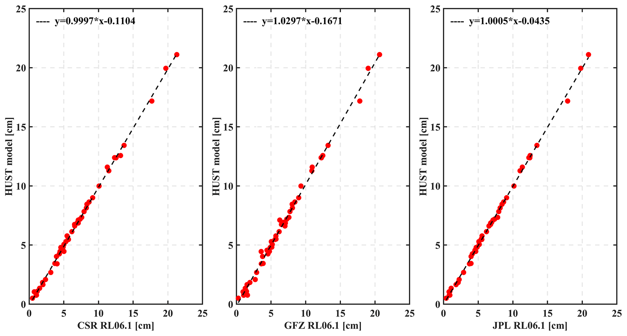
Figure 13 The annual amplitudes derived from CSR RL06.2, GFZ RL06.1, JPL RL06.1, and HUST-Grace2024 in the GRACE-FO solution during the period from 2018 to 2022. The x-axis value stands for the amplitude from the official solution, while the y-axis value stands for the value from the HUST solution. The dashed black line represents a linear fit line.

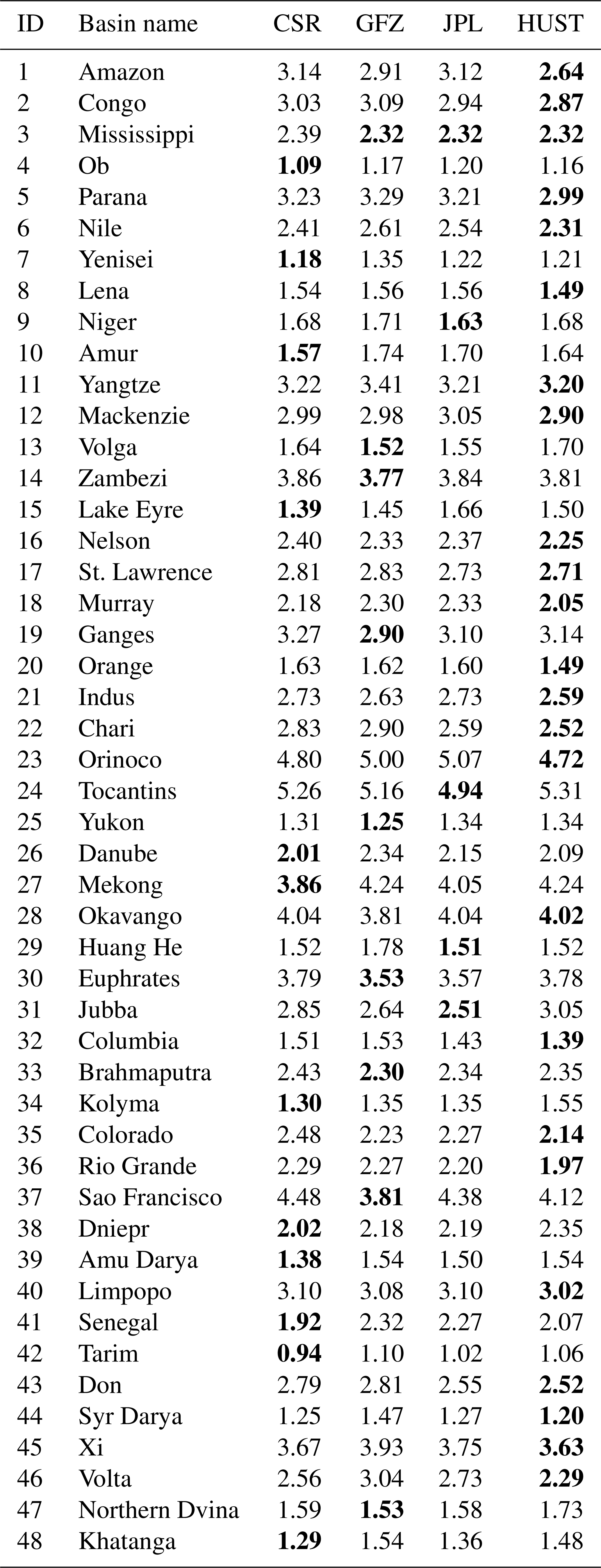
For a more quantitative analysis, we computed the terrestrial water storage anomaly (TWSA) variation time series following Eq. (13). As shown in Fig. 14, generally, the TWSA time series computed by our HUST-Grace2024 model is consistent with the latest GRACE-FO solution in eight representative basins such as the Amazon, Mekong, and Ob. These eight basins are selected based on their different latitudes for a general comparison. The comparison results demonstrate that our HUST-Grace2024 model has almost the same ability to maintain temporal signal when compared with the latest official GRACE-FO solutions. To make a more general comparison, as listed in Table 6, we also computed the TWSA residuals over the 48 representative basins. In addition, we also apply a high-pass filter to the TWSA residuals in order to mitigate the inter-annual variability in the TWSA residuals. In the large-scale basins like the Amazon, the rms values are 2.64, 3.14, 2.91, and 3.12 cm for HUST-Grace2024, CSR RL06.2, GFZ RL06.1, and JPL RL06.1, respectively. For small-scale basins such as the Orange, the rms values are 1.49, 1.63, 1.62, and 1.60 cm for HUST-Grace2024, CSR RL06.2, GFZ RL06.1, and JPL RL06.1, respectively. In addition, when compared with official GRACE-FO solutions, the HUST-Grace2024 model presents the smallest rms values over 68 % of these basins. The comparison of results also demonstrates the generally better performance of our HUST-Grace2024 model in reducing temporal noise when compared to the official GRACE-FO solutions.

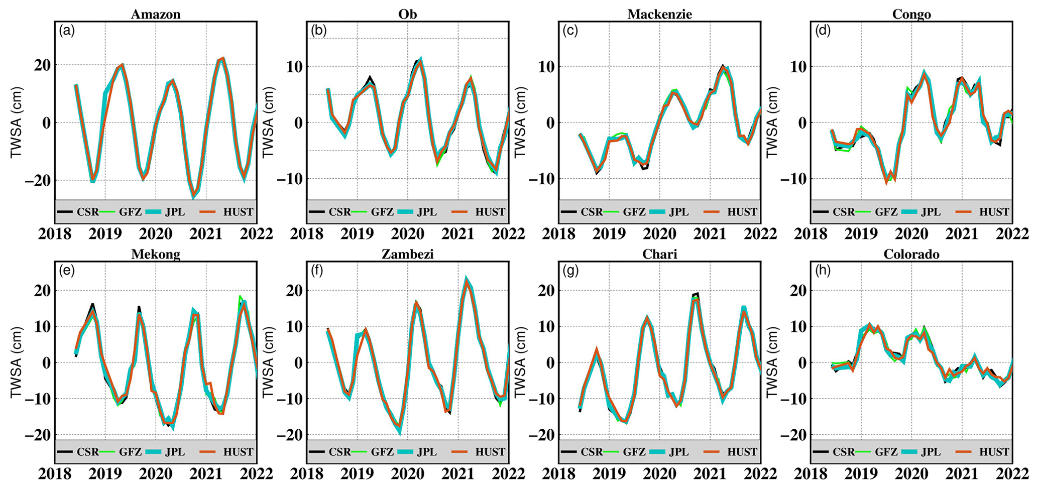
Figure 14 Terrestrial water storage anomaly (TWSA) variation time series of different basins during the period from 2018 to 2022 as derived from the latest official GRACE-FO solution and the HUST-Grace2024 model.

Table 6 The rms values (in centimeters) of 48 representative basins derived from the latest official GRACE-FO solution and the HUST-Grace2024 model. The bold value represents the minimum rms. Note that all rms values have been processed by a high-pass filter to mitigate the inter-annual signal variation in the EWH residual.

Overall, our HUST-Grace2024 model has good performance in both the spatial and the spectral domains when compared to the latest official solutions. It presents a balance between maintaining temporal signal and reducing temporal noise. In addition, the result related to GRACE-FO indicates the good performance of our hybrid processing chain in determining the temporal gravity field models for this mission, and it even presents more notable improvements when compared with the official GRACE solutions.

3.1.3 Comparing to HUST-Grace2020

In order to make a quantitative assessment of the contribution of different strategies in our hybrid processing chain, we perform a comparison between HUST-Grace2024 and a previous version of the HUST-Grace product, HUST-Grace2020. The comparison mainly focuses on the contribution of the newest AOD1B product AOD1B RL07 and the hybrid algorithm developed in HUST-Grace2024. Due to HUST-Grace2020 only spanning the period from January 2003 to July 2016, the comparison will only focus on GRACE solutions and exclude GRACE-FO solutions.

The details of processing strategies for different HUST products are summarized in Table 7. It is noted that only the main diagonal scale factor elements are estimated during HUST-Grace2020 determinations. The difference between HUST-Grace2020 and HUST-Grace2024prelimary can mainly be accounted for by the new stochastic model, and the difference between HUST-Grace2024prelimary and HUST-Grace2024 can mainly be accounted for by the new input AOD1B products. It should be kept in mind that the GRACE solution derived from CSR has the same fully populated scale factor matrix as HUST-Grace2024prelimary, which can also make an assessment of the contribution of the new stochastic model.

Table 7 Processing details differing between HUST-Grace2020 and HUST-Grace2024.

For an assessment of our strategies adopted in the hybrid processing chain, we select two monthly products derived from the different GRACE observation times shown in Figs. 15 and 16, which can help us to demonstrate the contribution of the newest AOD1B product and our refined processing chain described in the paper. The result derived from September 2009 can be regarded as a “good” observation time period, during which the GRACE satellites were both well temperature controlled. However, the result derived from April 2012 is usually regarded as a “bad” or “not so good” observation time period, as GRACE-B was without temperature control from this point on.

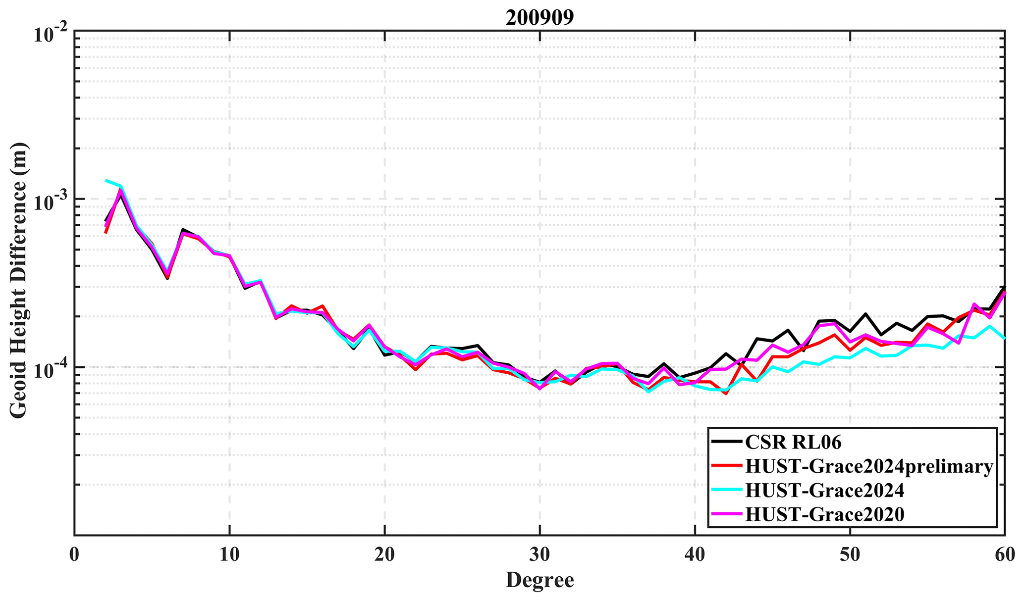
Figure 15 Geoid height difference per degree for different GRACE solutions in September 2009.

Figure 16 Geoid height difference per degree for different GRACE solutions in April 2012.

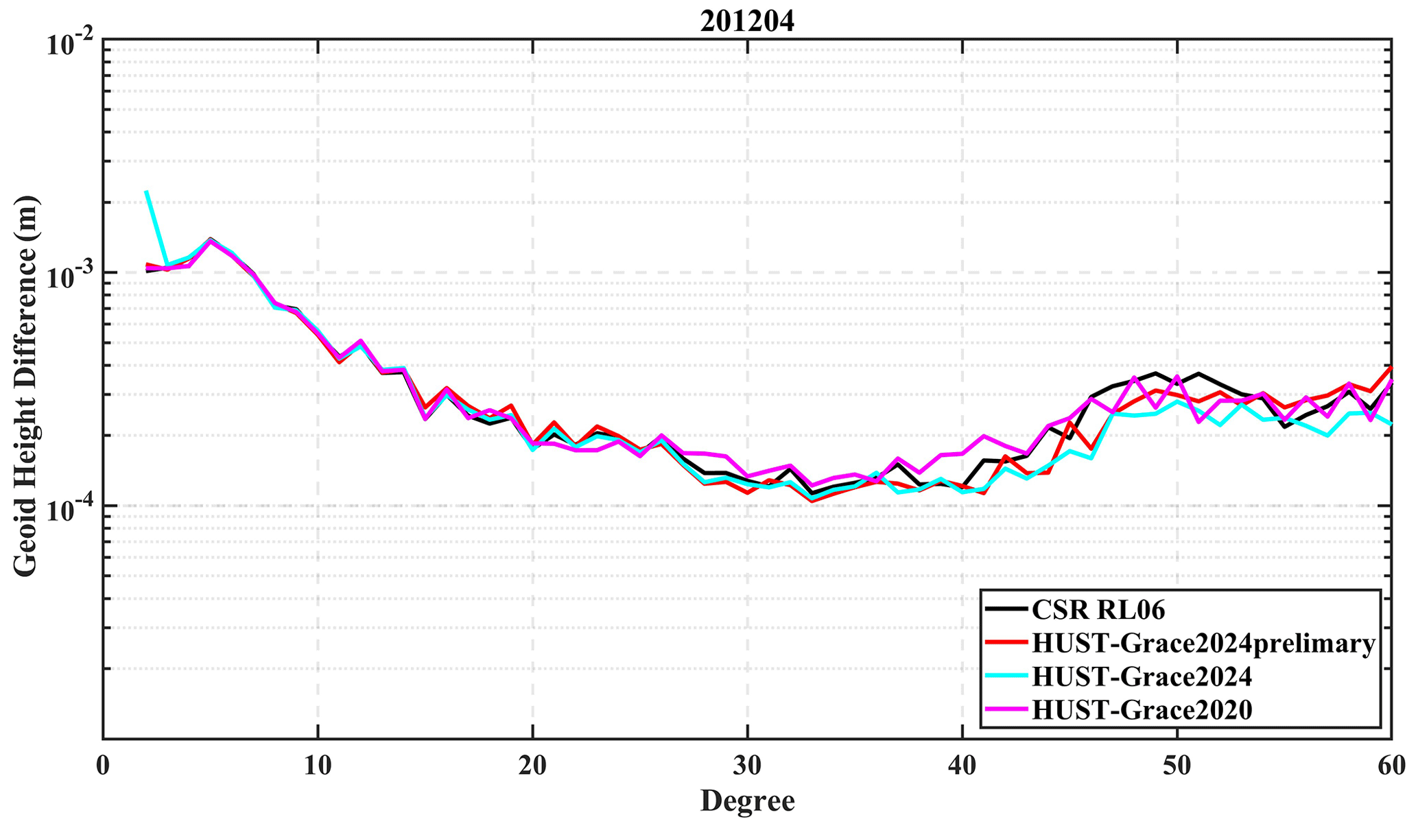
As shown in Fig. 15, the geoid height differences derived from different GRACE solutions are very similar below degree 40. The geoid height difference derived from HUST-Grace2020 is generally smaller than that derived from CSR, which mainly demonstrates that there is less temporal noise in HUST-Grace2020. The HUST-Grace2024prelimary model exhibits smaller geoid height differences than those from HUST-Grace2020 between degree 40 and degree 50, which indicates that our new stochastic model has a positive effect on reducing high-frequency noise. It should be noted that the adoption of AOD1B RL07 has a positive effect on reducing aliasing error during the temporal gravity field determination, especially above degree 40. However, as shown in Fig. 16, the geoid height difference is generally larger than that shown in Fig. 15, which demonstrates that the poor temperature control on GRACE-B has a negative impact on temporal gravity field determination. The geoid height difference derived from HUST-Grace2020 is slightly larger than that derived from CSR between degree 25 and degree 40 and is comparable with that from CSR between degree 40 and degree 60. It is noticeable that the geoid height difference derived from both HUST-Grace2024prelimary and HUST-Grace2024 is smaller than that from CSR between degree 40 and degree 60. This result indicates that the new stochastic model is still beneficial for the temporal gravity field determination during a “not so good” GRACE observation time period.

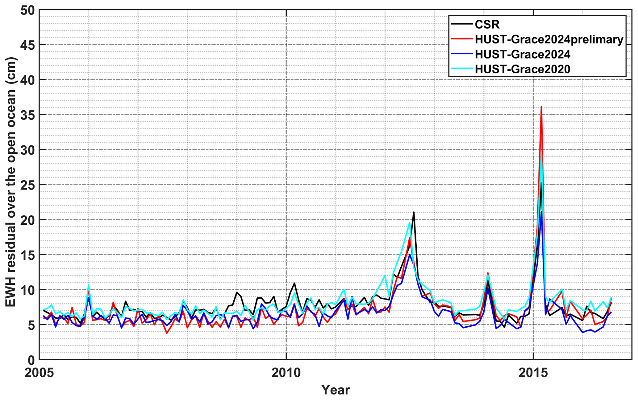
Figure 17 Equivalent water height (EWH) residual over a selected open-ocean series during the period from 2005 to 2016. The residual is computed by the EWH (without a filter) minus its climatology part (bias, amplitude, and trend).

Similar to the approach mentioned above, we still take the open-ocean residual as the criterion for the assessment of temporal noise in gravity field products. As shown in Fig. 17, the temporal noise in HUST-Grace2024prelimary is comparable with that in HUST-Grace2024 as well as with that in HUST-Grace2020 during 2005 and 2010; however, the temporal noise in HUST-Grace2024 is significantly less than that in other temporal gravity field products. The rms value is 8.23, 7.76, 6.94, and 8.59 cm for CSR, HUST-Grace2024prelimary, HUST-Grace2024, and HUST-Grace2020, respectively. Compared to HUST-Grace2020, the reduction in temporal noise is 9.6 % and 19.2 % for HUST-Grace2024prelimary and HUST-Grace2024, respectively.

4 Data availability

The GRACE level 1B data in this study are freely available at http://isdcftp.gfz-potsdam.de (Wen et al., 2019), and the kinematic orbits are provided by ITSG at http://ftp.tugraz.at (Suesser-Rechberger et al., 2019). The HUST-Grace2024 model is available at https://doi.org/10.5880/ICGEM.2024.001 (Zhou et al., 2024).

5 Conclusions

On the basis of a new hybrid processing chain, we developed a new series of temporal gravity field models called HUST-Grace2024. The highlights of this hybrid processing chain include the improved GRACE and GRACE-FO L1B datasets, the updated background models, the new pre-processing chain, the hybrid data-weighting method, and the updated accelerometer scale factor matrix.

While determining our HUST-Grace2024 temporal gravity field model, the latest GRACE and GRACE-FO L1B datasets were used, including RL03 data for GRACE and RL04 data for GRACE-FO. The background force models were also updated, including the static gravity field GOCO06s and the newest atmosphere and ocean de-aliasing product AOD RL07. Meanwhile, to comprehensively consider the color noise at different frequencies, the empirical kinematic parameters as well as the stochastic model were applied as a hybrid weighting method. The hybrid weighting method presents notable improvements when compared to the traditional weighting method. For the accelerometer scale factor matrix, we fully considered the misalignment between the SRF and the AF as well as the non-orthogonality of the three AF axes. The scale factor estimations at the main diagonal line are more stable for the GRACE mission than for the GRACE-FO mission, especially in the along-track direction. In contrast, the scale factor estimations off the main diagonal line are similar between GRACE and GRACE-FO, which reflects the similar performance of alignment or orthogonality of the axes related to accelerometers.

In the hybrid processing chain, we specially developed a hybrid outlier detection method for the pre-processing procedure. The method is based on the SOE file and the inter-satellite pointing angles. Based on several practical computations for the real GRACE observations, it is advisable to set a threshold of pointing angles at 50 mrad and to use a 100 s margin to detect outliers in range-rate observations, while setting the threshold at 20 mrad and using a 600 s margin for accelerometer data. The updated pre-processing strategy ensures accurate exclusion of outliers in observations on the one hand and improves the quality of temporal gravity field estimations on the other.

Further, the newly developed temporal gravity field model HUST-Grace2024 was compared with the latest official solutions, including CSR RL06, GFZ RL06, and JPL RL06 for GRACE (RL06.1 for GRACE-FO derived from GFZ and JPL and RL06.2 for GRACE-FO derived from CSR). In the spectral domain, the cumulative geoid height difference during the period from 2005 to 2016 reflects the lower noise level of HUST-Grace2024, with a noise reduction of 3.0 % to 27.2 % when compared to the official GRACE solutions. Even more notable noise reductions are observed for GRACE-FO solutions, which vary from 17.6 % to 46.9 %. The results present the better efficiency of our hybrid processing chain for the GRACE-FO mission than for the GRACE mission. In the spatial domain, a noticeable temporal noise reduction is observed over the open ocean in HUST-Grace2024. The mean rms values over the open ocean are 132.3, 228.1, 209.2, and 118.0 cm for CSR RL06, JPL RL06, GFZ RL06, and HUST-Grace2024, respectively. As for GRACE-FO solutions, they are 235.2, 488.6, 390.3, and 177.7 cm, respectively. The annual amplitudes of 48 major basins derived from HUST-Grace2024 show good agreement with those derived from the official solutions, while over 68 % of basins present the smallest rms values when compared to the official solutions. The comparisons in the spectral and spatial domains indicate that our updated hybrid process chain can result in better GRACE and GRACE-FO monthly gravity field estimations.

Overall, the updated pre-processing method gives us an insight into observation data, especially enabling exclusion of outliers during satellite onboard events. Meanwhile, the hybrid weighting method leads to a better understanding of frequency-dependent noise in the real GRACE and GRACE-FO observations. As described in Flechtner et al. (2016), Chen et al. (2020), and Zhou et al. (2023), the force model errors and accelerometer errors have been the dominant limiting factors for GRACE-FO. Our hybrid processing chain can help us understand the stochastic characteristics of instrument noise and develop a series of temporal gravity fields based on the observation data from GRACE-FO.