Visibility-derived aerosol optical depth over global land from 1959 to 2021

Long-term and high spatial resolution aerosol optical depth (AOD) data are essential for climate change detection and attribution. Global ground-based AOD observations are sparsely distributed, and satellite AOD retrievals have a low temporal frequency as well low accuracy before 2000 over land. In this study, AOD at 550 nm is derived from visibility observations collected at more than 5000 meteorological stations over global land regions from 1959 to 2021. The AOD retrievals (550 nm) of the Moderate Resolution Imaging Spectroradiometer (MODIS) on board the Aqua Earth observation satellite are used to train the machine learning model, and the ERA5 reanalysis boundary layer height is used to convert the surface visibility to AOD. Comparisons with an independent dataset (AERONET ground-based observations) show that the predicted AOD has a correlation coefficient of 0.55 at the daily scale. The correlation coefficients are higher at monthly and annual scales, which are 0.61 and 0.65, respectively. The evaluation shows consistent predictive ability prior to 2000, with correlation coefficients of 0.54, 0.66, and 0.66 at the daily, monthly, and annual scales, respectively. Due to the small number and sparse visibility stations prior to 1980, the global and regional analysis in this study is from 1980 to 2021. From 1980 to 2021, the mean visibility-derived AOD values over global land areas, the Northern Hemisphere, and the Southern Hemisphere are 0.177, 0.178, and 0.175, with a trend of −0.0029 per 10 years, −0.0030 per 10 years, and −0.0021 per 10 years from 1980 to 2021. The regional means (trends) of AOD are 0.181 (−0.0096 per 10 years), 0.163 (−0.0026 per 10 years), 0.146 (−0.0017 per 10 years), 0.165 (−0.0027 per 10 years), 0.198 (−0.0075 per 10 years), 0.281 (−0.0062 per 10 years), 0.182 (−0.0016 per 10 years), 0.133 (−0.0028 per 10 years), 0.222 (0.0007 per 10 years), 0.244 (−0.0009 per 10 years), 0.241 (0.0130 per 10 years), and 0.254 (0.0119 per 10 years) in Eastern Europe, Western Europe, Western North America, Eastern North America, Central South America, Western Africa, Southern Africa, Australia, Southeast Asia, Northeast Asia, Eastern China, and India, respectively. However, the trends decrease significantly in Eastern China (−0.0572 per 10 years) and Northeast Asia (−0.0213 per 10 years) after 2014, with the larger increasing trend found after 2005 in India (0.0446 per 10 years). The visibility-derived daily AOD dataset at 5032 stations over global land from 1959 to 2021 is available from the National Tibetan Plateau/Third Pole Environment Data Center (https://doi.org/10.11888/Atmos.tpdc.300822) (Hao et al., 2023).

1 Introduction

Atmospheric aerosols are composed of solid and liquid particles suspended in the atmosphere. Aerosol particles are directly emitted into the atmosphere or formed through gas–particle transformation (Calvo et al., 2013) with diverse shapes and sizes (Fan et al., 2021), optical properties, and components (Liao et al., 2015; Zhang et al., 2020; Li et al., 2022). Most atmospheric aerosols are concentrated in the troposphere, especially in the boundary layer (Liu et al., 2022), with a high concentration near emission sources (Kulmala et al., 2004), and a small portion are distributed in the stratosphere. Atmospheric aerosols severely impact the atmospheric environment and human health. They deteriorate air quality, reduce visibility, and cause other environmental issues (Wang et al., 2012; Boers et al., 2015). They also impair human health or the conditions of organisms by increasing the incidence of cardiovascular and respiratory disease and mortality rates (Chafe et al., 2014; Yang et al., 2022). The Global Burden of Disease study shows that global exposure to ambient PM_2.5 (particulate matter suspended in air with an aerodynamic diameter of less than 2.5 µm) resulted in 0.37 million deaths and 9.9 million disability-adjusted life years (Chafe et al., 2014).

Aerosols are inextricably linked to climate change. Atmospheric aerosols alter the Earth's energy budget and affect the climate (Li et al., 2022). They cool the surface and heat the atmosphere by scattering and absorbing solar radiation (Forster et al., 2007; Chen et al., 2022). Aerosols, such as black carbon and brown carbon, also absorb solar radiation (Bergstrom et al., 2007), heat the local atmosphere, and suppress or stimulate convective activities (Ramanathan et al., 2001; Sun and Zhao, 2020). Furthermore, aerosols alter the optical properties and life span of clouds (Albrecht, 1989). Atmospheric aerosols strongly affect regional and global short-term and long-term climates through direct and indirect effects (Mcneill, 2017).

Tropospheric aerosols are considered the second-largest forcing factor for global climate change (Li et al., 2022), and they reduce the warming attributable to greenhouse gases by −0.5 °C (IPCC, 2021). However, aerosols are also regarded as the largest contributor to the uncertainty of present-day climate change attribution (IPCC, 2021). The uncertainties are caused by deficiencies in the descriptions of global aerosol optical properties (such as scattering and absorption) and of microphysical properties (such as size and component) as well as by their impact on cloud and precipitation, further affecting the estimation of aerosol radiative forcing (Lee et al., 2016; IPCC, 2021). Therefore, it is crucial to have sufficient aerosol observations. In aerosol measurements, aerosol optical depth (AOD) is often used to describe its column properties, which represents the vertical integration of aerosol extinction coefficients. AOD is an important physical quantity for estimating the content, atmospheric pollution, and climatology of aerosols (Zhang et al., 2020).

AOD data usually come from ground-based and satellite-borne remote sensing observations. Both methods have advantages and disadvantages. Ground-based lidar observation is an active remote sensing technology. Lidar generally emits laser and receives backscattered signals to invert the extinction coefficient of aerosols at different heights (Klett, 1985). By using the depolarization ratio, the type of aerosol, such as fine particles or dust, can be distinguished (Bescond et al., 2013). The AOD within a certain height can be calculated by integrating the extinction coefficients; however, scattering signals are usually not received near the ground, leading to blind spots (Singh et al., 2019). At present, there are many global and regional ground-based lidar networks which provide important support regarding vertical changes in aerosols, such as the NASA Micro-Pulse Lidar Network (MPLNET) in the early 1990s (Welton et al., 2002), the European Aerosol Research Lidar Network (EARLINET) since 2000 (Bösenberg et al., 2003), and the Latin American Lidar Network (LALINET) since 2013 (Guerrero-Rascado et al., 2016).

Ground-based remote sensing observations supply aerosol loading data (such as AOD) by measuring the attenuation of radiation from the top of the atmosphere to the surface (Holben et al., 1998). This type of observation mainly uses weather-resistant automatic sun- and sky-scanning spectral radiometers to retrieve optical and microphysical aerosol properties (Che et al., 2014). The Aerosol Robotic Network (AERONET) is a popular global network established by NASA and multiple international partners that provides high-quality and high-frequency aerosol optical and microphysical properties under various geographical and environmental conditions (Holben et al., 1998; Dubovik et al., 2000). The AERONET observations are extensively used to validate satellite remote sensing observations and model simulations as well as for climatology studies (Dubovik et al., 2002b). There are many regional networks of sun photometers, such as the Maritime Aerosol Network (MAN), which uses a handheld sun photometer to collect data over the ocean and is merged into AERONET (Smirnov et al., 2009); the China Aerosol Robot Sun Photometer Network (CARSNET) (Che et al., 2009); the Canadian subnetwork of AERONET (AEROCAN) (Bokoye et al., 2001); Aerosol characterization via Sun photometry: Australian Network (AeroSpan) (Mukkavilli et al., 2019); and the sky radiometer network (SKYNET) in Asia and Europe (Kim et al., 2004; Nakajima et al., 2020). Another very valuable global network is the NOAA/ESRL Federated Aerosol Network (FAN), which uses integrated nephelometers distinct from sun photometers, mainly located in remote areas, providing background aerosol properties over 30 sites (Andrews et al., 2019).

Satellite remote sensing is a space-based method that can provide aerosol properties worldwide. With the development of satellite remote sensing technology since the 1970s, aerosol distributions can be extracted with the advantage of sufficient real-time and global coverage from multiple satellite sensors (Kaufman and Boucher, 2002; Anderson et al., 2005). The Advanced Very High Resolution Radiometer (AVHRR) is the earliest sensor used for retrieving AOD over ocean (Nagaraja Rao et al., 1989). The Moderate Resolution Imaging Spectroradiometer (MODIS), on board the Terra (launched in 1999) and Aqua (launched in 2002) satellites, is a popular sensor with 36 channels, which has been used for AOD retrieval over both ocean and land based on the dark target and deep blue algorithms (Remer et al., 2005; Levy et al., 2013). The latest MODIS AOD data version is Collection 6.1, which provides global AOD over 20 years (Wei et al., 2019). There are also many other satellite sensors that can be used to retrieve AOD, such as the Polarization and Directionality of the Earth's Reflectances (POLDER) during 1996–1997, 2003, and 2004–2013 (Deuzé et al., 2000); the Sea-viewing Wide Field-of-view Sensor (SeaWIFS) during 1997–2007 (O'Reilly et al., 1998); and the Multi-angle Imaging Spectroradiometer (MISR) on Terra since 1999 (Diner et al., 1998). The Cloud-Aerosol Lidar with Orthogonal Polarization (CALIOP) has also derived aerosols in the vertical direction since 2006 (Winker et al., 2009).

These measurements provide important data for studying the global and regional spatiotemporal variabilities and climate effect of aerosols. However, ground-based remote sensing observations only provide aerosol properties with low spatial coverage. There were only about 150 ground stations worldwide in 2002, and even fewer sites were available for climate analysis (Holben et al., 1998; Chu et al., 2002), which limited aerosol climate research by spatial coverage (Bright and Gueymard, 2019). Satellite remote sensing overcomes the limitations of spatial coverage. The AVHRR has been used to retrieve AOD since 1980, but it is limited by a low number of channels, low spatial resolution, and insufficient validation through ground-based observations before 2000 (Hsu et al., 2017). Many studies have only investigated the trends and distributions of aerosols after 2000 (Bösenberg and Matthias, 2003; Winker et al., 2013; Xia et al., 2016; Tian et al., 2023) because of the lack of long-term and global-cover AOD products, which is a bottleneck for aerosol climate change detection and attribution.

To overcome these limitations and enrich aerosol data, alternative observation data could be utilized to derive AOD. Atmospheric horizontal visibility is a suitable alternative (Wang et al., 2009; Zhang et al., 2020) because it has the advantages of long-term records with a large number of stations worldwide.

Atmospheric visibility is a physical quantity that describes the transparency of the atmosphere through manual and automatic observations; automatic observations of visibility usually measure atmospheric extinction (scattering coefficient and transmissivity). Koschmieder (1924) first proposed the relationship between the meteorological optical range and the total optical depth. Elterman (1970) further established a formula between AOD and visibility by assuming an exponential decrease in aerosol concentration with altitude, considering the extinction of molecules and ozone to analyze air pollution, which was called “the Elterman model”. Qiu and Lin (2001) corrected the Elterman model by considering the influence of water vapor and used two water vapor pressure correction coefficients to retrieve the AOD of 16 stations in China in 1990. Wang et al. (2009) analyzed the trend in AOD using visibility-based retrievals from 1973 to 2007 over land. Lin et al. (2014) retrieved the AOD in Eastern China in 2006 using visibility and aerosol vertical profiles provided by GEOS-Chem. Wu et al. (2014) and Zhang et al. (2017) parameterized the constants in the Elterman model and used satellite-retrieved AOD to solve the parameters in the models at different stations in order to retrieve the long-term AOD in China.

Zhang et al. (2020) reviewed the methods of visibility retrieval of AOD, indicating that visibility-based retrieval of AOD can compensate for the shortcomings of long-term aerosol observation data. Simultaneously, various parameters, such as station altitude, consistency in visibility data, and water vapor and aerosol vertical profiles (scale height), were discussed, with modified suggestions being proposed. These studies have enriched AOD data regionally and have also enriched aerosol data to some extent. At present, there are very few studies on global visibility-retrieved AOD for analyzing the climatology of aerosols.

The two physical quantities of visibility and AOD have similarities and differences that make it challenging to retrieve AOD from visibility. Visibility represents the maximum horizontal visible distance near the surface which is impaired by surface aerosols, while AOD represents the total column attenuation of solar radiation by aerosols from the surface to the top of the atmosphere. The visibility of automatic observations is dependent on the local horizontal atmospheric extinction. Visibility does not have a simple linear relationship with meteorological factors. Obtaining the vertical structure of aerosols is the greatest challenge, as it is not a simple hypothetical curve in complex terrain and circulation conditions (Zhang et al., 2020). These limitations make it more complex to derive AOD. Machine learning methods can effectively address complex nonlinear relationships between variables and have been widely applied in remote sensing and climate research fields. Li et al. (2021) used the random forest method to predict PM_2.5 in Iraq and Kuwait based on satellite AOD during 2001–2018. Kang et al. (2022) applied LightGBM and random forest to estimate AOD over East Asia, and the results showed consistency with AERONET. Dong et al. (2023) derived aerosol single-scattering albedo from visibility and satellite AOD over 1000 global stations. Hu et al. (2019) used a deep learning method to retrieve horizontal visibility from MODIS AOD. These studies have confirmed the ability of machine learning to effectively solve complex relationships among variables. Previous studies were mostly conducted at the regional or national scale, with few studies carried out at the global scale. Thus, it is feasible to derive AOD from atmospheric visibility over global land by using the machine learning method.

Figure 1 Study area (a) and meteorological stations (b) at the daily, monthly, and annual scales. The number of meteorological stations (purple circles) is 5032. The number of AERONET sites (cyan circles) is 395. The boxed regions labeled with numbers 1–12 are Western Europe, Eastern Europe, Western North America, Eastern North America, Central South America, Western Africa, Southern Africa, Australia, Southeast Asia, Northeast Asia, Eastern China, and India, respectively.

In this study, we propose a machine learning method to derive AOD, where satellite AOD is the target value and visibility and other related meteorological variables are the predictors. We explain the model's robustness, evaluate the model's predictive ability, and validate the model's predictions using independent ground-based AOD, satellite retrievals, and reanalysis AOD. Furthermore, we analyze the mean AOD and the AOD trend across global land and regions. A station-scale dataset of long-term AOD is generated. Section 2 introduces the data and method. Section 3 presents the evaluation and validation of the visibility-derived AOD as well as a discussion of the distribution and trends at global and regional scales. Finally, Sect. 5 presents the conclusions. This study is aimed at supporting the research of aerosols in climate change detection and attribution.

2 Data and method

2.1 Study area

The study area is global land. A total of 5032 meteorological stations and 395 AERONET sites are selected in this study, as shown in Fig. 1. For the regional analysis, 12 regions are selected, i.e., Eastern Europe, Western Europe, Western North America, Eastern North America, Central South America, Western Africa, Southern Africa, Australia, Southeast Asia, Northeast Asia, Eastern China, and India, and the number of stations in each region is 187, 494, 390, 1759, 132, 72, 78, 86, 76, 140, 26, and 51, respectively. The meteorological observation data including visibility are available from 1959. The time period for the global and regional analysis is from 1980 to 2021, during which the visibility observations are sufficient with a uniform spatial distribution. As shown in Fig. 1, the number of active stations exceeded 2000 during the period 1980–1990, and the number of active stations has exceeded 3000 since the year 2000.

2.2 Meteorological data

The ground-based hourly meteorological data from 1959 to 2021 are collected from 5032 meteorological stations at airports over land, which can be downloaded at https://mesonet.agron.iastate.edu/ASOS (last access: 9 July 2024). Over 1000 stations belong to the Automated Surface Observing System (ASOS), and others are sourced from airport reports around the world. The visibility measurements can be divided into automatic observations and manual observations. Automatic visibility observations reduce errors associated with human involvement in data collection, processing, and transmission. The visibility and other meteorological data are extracted from the Meteorological Terminal Aviation Routine Weather Report (METAR). The World Meteorological Organization (WMO) sets guidelines for METAR reports, including report format, encoding, observation instruments and methods, data accuracy, and consistency, which ensures the consistency and comparability of METAR reports globally. Some international regulations can be referenced at https://community.wmo.int/en/implementation-areas-aeronautical-meteorology-programme (last access: 9 July 2024).

The daily average visibility is calculated using the harmonic mean in Eq. (1). The reciprocal of visibility is proportional to the extinction coefficient (Wang et al., 2009). Experiments have shown that harmonic average visibility can better detect the weather phenomena than arithmetic average visibility when visibility declines quickly. Therefore, daily visibility will have greater representativeness:

$$\begin{array}{}\text{(1)}& V=n/\left({\displaystyle \frac{\mathrm{1}}{V_{\mathrm{1}}}}+{\displaystyle \frac{\mathrm{1}}{V_{\mathrm{2}}}}+\mathrm{\dots }+{\displaystyle \frac{\mathrm{1}}{V_n}}\right),\end{array}$$

where V is the harmonic mean visibility; n is the daily record number; and V₁, V₂,…V_n are the individual hourly visibility.

In addition to hourly visibility (VIS), other variables closely related to aerosol properties are selected, including relative humidity (RH), dew point temperature (DT), temperature (TMP), wind speed (WS), and sea-level pressure (SLP). These variables are chosen because air temperature affects atmospheric stability and the rate of secondary particle formation, humidity influences the size and hygroscopic growth, and wind speed and pressure significantly impact the transport and deposition of aerosols. Sky conditions (cloud amount) and hourly precipitation are also selected to remove the records of extensive cloud cover and precipitation.

We processed the meteorological data as follows. Records with a high missing value ratio are eliminated (Husar et al., 2000). When of sky conditions have over 80 % overcast or fog, the records are eliminated, although such situations occur less than 1 % of the time over land (Remer et al., 2008). Records with 1 h precipitation greater than 0.1 mm are eliminated. We calculate the temperature dew point difference (dT). Low-visibility records under “blowing snow” weather are eliminated at high latitudes (> 65° N) when wind speed is greater than 4.5 m s⁻¹ (Husar et al., 2000). When the RH is greater than 90 %, it is impossible to distinguish whether it is fog, haze, or both and even whether it is precipitation. Therefore, records with RH greater than or equal to 90 % are eliminated. When the RH is less than 30 %, the hygroscopic effect of aerosols is very low or even negligible. When the RH is between 30 % and 90 %, the hygroscopic effect of aerosols is high, and visibility is converted to dry visibility (Y. Yang et al., 2021), as shown in Eq. (2). At least 3 hourly records of meteorological variables are required when calculating the daily average (n ≥ 3):

$$\begin{array}{}\text{(2)}& \mathrm{VISD}=\mathrm{VIS}/(\mathrm{0.26}+\mathrm{0.4285}\cdot \log (\mathrm{100}-\mathrm{RH}\left)\right),\end{array}$$

where VISD is the dry visibility.

2.3 Boundary layer height

The hourly boundary layer height (BLH) data from 1980 to 2021 are available from the Fifth Generation Reanalysis of the European Medium-Range Weather Forecast Center (ERA5) with a resolution of 0.25° × 0.25° (https://cds.climate.copernicus.eu, last access: 9 July 2024), which is the successor of ERA-Interim and has undergone various improvements (Hersbach et al., 2020). The atmospheric boundary layer is the layer closest to the Earth's surface. It exhibits complex turbulence activities, and its height undergoes significant diurnal variation. The boundary layer plays a crucial role in regulating and adjusting the distribution of atmospheric aerosols, such as vertical distribution, concentration changes, transport, and deposition (Ackerman et al., 1995). The boundary layer height serves as an approximate measure of the scale height for aerosols (Zhang et al., 2020).

Compared with observations of 300 stations around the world from 2012 to 2019, the ERA5 BLH is underestimated by 131.96 m, and it is closest to the observations when compared with JRA-55 and NECP-2 BLH (Guo et al., 2021). The hourly BLH data are temporally and spatially matched with visibility and other meteorological data before calculating the daily average.

Figure 2 Flowchart for deriving aerosol optical depth (AOD).

Because the reciprocal of visibility is proportional to the extinction coefficient and positively related to AOD (Wang et al., 2009), we calculate the reciprocal of visibility (VISI) and the reciprocal of dry visibility (VISDI). Due to the influence of boundary layer height on the vertical distribution of particles (Zhang et al., 2020), we calculate the product (VISDIB) of VISDI and BLH. Therefore, the predictor (Fig. 2) is composed of 11 variables (TMP, Td, dT, RH, SLP, WS, VIS, BLH, VISI, VISDI, and VISDIB).

2.4 MODIS AOD products

Satellite daily AOD data are available from the Moderate Resolution Imaging Spectroradiometer (MODIS) Level 3 Collection 6.1 AOD products of the Aqua (MYD09CMA) satellite from 2002 to 2021 and the Terra (MOD09CMA) satellite from 2000 to 2021 with a spatial resolution of 0.05° × 0.05° at a wavelength of 550 nm (https://ladsweb.modaps.eosdis.nasa.gov, last access: 9 July 2024). Terra (passing at 10:30 local time) and Aqua (passing at 13:30 local time) were successfully launched in December 1999 and May 2002, respectively. MODIS, carried on the Terra and Aqua satellites, is a crucial instrument in the NASA Earth Observing System program, which is designed to observe global biophysical processes (Salomonson et al., 1987). The 2330 km wide swath of the orbit scan can cover the entire globe every 1–2 d. MODIS has 36 channels and more spectral channels than previous satellite sensors (such as AVHRR). The spectrum ranges from 0.41 to 15 µm, representing three spatial resolutions: 250 m (2 channels), 500 m (5 channels), and 1 km (29 channels). The aerosol retrievals use seven of these channels (0.47–2.13 µm) to retrieve aerosol characteristics and use additional channels in other parts of the spectrum to identify clouds and river sediments. Therefore, it has the ability to characterize the spatial and temporal characteristics of the global aerosol field.

The MODIS aerosol product actually uses different algorithms to retrieve aerosols over land. The dark target (DT) algorithm is applied to densely vegetated areas because the surface reflectance over dark-target areas is lower in the visible channels and has nearly fixed ratios with the surface reflectance in the shortwave and infrared channels (Levy et al., 2007, 2013). The deep blue (DB) algorithm was originally applied to bright land surfaces (such as deserts) and later extended to cover all cloud-free and snow-free land surfaces (Hsu et al., 2006, 2013). The MODIS Collection 6.1 aerosol product was released in 2017, incorporating significant improvements in radiometric calibration and aerosol retrieval algorithms.

The aerosol retrievals are usually evaluated by the expected error. For the DT algorithm, the expected error is ± (0.05 ± 15 % AOD_AERONET). The coverage of retrieval products varies by season based on the DT algorithm over land. Higher spatial coverage is observed in August and September, reaching 86 %–88 %. During December and January, due to the presence of permanent ice and snow cover in high-latitude regions of the Northern Hemisphere, the spatial coverage is 78 %–80 %. Thus, challenges remain in retrieving AOD values in high-latitude regions (Wei et al., 2019). However, visibility observations are available in high-latitude regions, thereby partially addressing the lack in these regions. In this study, the Terra and Aqua MODIS AOD data are temporally and spatially matched with the meteorological stations. Aqua MODIS AOD is used as the target when training the model, and Terra MODIS AOD is used in the evaluation and validation of the model results, as shown in the flowchart (Fig. 2).

2.5 Ground-based AOD

Ground-based 15 min AOD observations are available from the Aerosol Robotic Network (AERONET) Version 3.0 Level 2.0 product at 395 sites (Fig. 1), which can be downloaded from https://aeronet.gsfc.nasa.gov (last access: 9 July 2024). The AERONET program is a federation of ground-based remote sensing aerosol networks established by NASA and PHOTONS, including many subnetworks (such as AeroSpan, AEROCAN, NEON, and CARSNET). The sun photometer (CE-318) measures spectral sun and sky irradiance in the 340–1020 nm spectral range. AERONET has three levels of AOD products: Level 1.0 (unscreened), Level 1.5 (cloud screened), and Level 2.0 (cloud screened and quality assured). Compared with Version 2, the Version 3 Level 2.0 database has undergone further cloud screening and quality assurance, which is generated based on Level 1.5 data with pre- and post-calibration and temperature adjustment and is recommended for formal scientific research (Giles et al., 2019). AERONET provides AOD products at wavelengths of 440, 675, 870, and 1020 nm. When the aerosol loading is low, the error is significant. When the AOD at 440 nm wavelength is less than 0.2, the error is 0.01, which is equivalent to the error of the absorption band in the total optical depth (Dubovik et al., 2002a). The total uncertainty in AOD under cloud-free conditions is less than ± 0.01 when the wavelength is more than 440 nm and ± 0.02 when the wavelength is less than 440 nm (Holben et al., 1998). AERONET AOD is usually considered the “true” value. The AOD at 440 nm and the Ångström index at 440–675 nm are used to calculate AOD at 550 nm (not provided by AERONET), as shown in Eq. (3):

$$\begin{array}{}\text{(3)}& {\mathit{\tau }}_{\mathrm{550}}={\mathit{\tau }}_{\mathrm{440}}{\left({\displaystyle \frac{\mathrm{550}}{\mathrm{440}}}\right)}^{-\mathit{\alpha }},\end{array}$$

where τ₄₄₀ and τ₅₅₀ are the AOD at a wavelength of 440 and 550 nm, respectively, and α is the Ångström index.

The daily average AOD requires at least two observations within 1 h (± 30 min) of Aqua and Terra transit time (Wei et al., 2019). The matching conditions between AERONET sites and meteorological stations are (1) a distance of less than 0.5° and (2) at least 3 years of observations. Finally, a total of 395 sites are selected.

2.6 AOD reanalysis dataset

The monthly AOD (550 nm) dataset of Modern-Era Retrospective Analysis for Research and Applications Version 2 (MERRA-2) from 1980 to 2021 is a NASA reanalysis of the modern satellite era produced by NASA's Global Modeling and Assimilation Office with a spatial resolution of 0.5° × 0.625° (Gelaro et al., 2017) and is available at https://disc.gsfc.nasa.gov (last access: 9 July 2024). MERRA-2 AOD uses an analysis splitting technique to assimilate AOD data at 550 nm. The assimilated AOD observations include (1) AOD retrievals from AVHRR (1979–2002) over global ocean, (2) AOD retrievals from MODIS on Terra (2000–present) and Aqua (2002–present) over global land and ocean, (3) AOD retrievals from MISR (2000–2014) over bright and desert surfaces, and (4) direct AOD measurements from ground-based AERONET sites (1999–2014) (Gelaro et al., 2017). The monthly MERRA-2 AOD is used to evaluate the model's predictive ability before 2000 and after 2000.

2.7 Decision tree regression

2.7.1 Feature selection

Although a multidimensional dataset can provide as much potential information as possible for AOD, irrelevant and redundant variables can also introduce significant noise in the model and reduce the model's accuracy and stability (Kang et al., 2021; Dong et al., 2023). Therefore, the F test is used to search for the optimal feature subset in the predictor, aiming to eliminate irrelevant or redundant features and select truly relevant features, which helps to simplify the model's input and improve the model's prediction ability (Dhanya et al., 2020). The F test is a statistical test that gives an f score (= −log(p), p represents the degree to which the null hypothesis is not rejected) by calculating the ratio of variances. In this study, we calculate the ratio of variance between the predictors and the target, and the features are ranked based on the f-score values. A higher f-score value means that the distances between the predictors and the target are less and the relationship is closer; thus, the feature is more important. We set p = 0.05. When the score is less than −log(0.05), the variable in the predictors is not considered.

2.7.2 Data balance

When the weather is clear, the AOD value is small (AOD < 0.5), the variability of AOD is small, and the data are concentrated near the mean value. When there is heavy pollution, the AOD value is large (AOD > 0.5). Compared with clear sky, the AOD sequence will show “abnormal” large values with low frequency, which is a phenomenon of imbalanced AOD data. When dealing with imbalanced datasets, because of the tendency of machine learning algorithms to perform better on the majority class and overlook the minority class, the model may be underfit (Chuang and Huang, 2023). Data augmentation techniques are commonly employed to address the issue in imbalanced data by applying a series of transformations or expansions to generate new training data, thereby increasing the diversity and quantity of the training data of the minority class.

The Adaptive Synthetic Sampling (ADASYN) is a data augmentation technique specifically designed to address the data imbalance problem (He et al., 2008; Mitra et al., 2023). It is an extension of the Synthetic Minority Over-sampling Technique (SMOTE) algorithm (Fernández et al., 2018). The goal of ADASYN is to generate synthetic sample data for the minority class so as to increase its representation in the dataset. ADASYN, which adaptively adjusts the generation ratio of synthetic samples based on the density distribution of sample data, improves the dataset balance and enhances the performance of machine learning models in dealing with imbalanced data.

The processing of imbalanced data includes the following: (1) AOD sequences are classified into three types based on percentile (0 %–1 %, 2 %–98 %, 99 %). (2) When the mean of the third type of AOD is greater than 5 times the standard deviation of the second type, it is considered an imbalanced sequence. These data, with a total amount of less than 5 % of the sample, are imbalanced data. (3) Then, synthetic samples are generated with a 10 % upper limit of the original samples.

2.7.3 Decision tree regression model

The decision tree is a machine learning algorithm based on a tree-like structure used to solve classification and regression problems. We use a regression tree algorithm to construct a regression model by analyzing the mapping relationship between object attributes (predictor) and object values (target). The internal nodes have binary tree structures with feature values of “yes” and “no”. In addition, each leaf node represents a specific output for a feature space. The advantages of the regression tree include the ability to handle continuous features and the ease of understanding the tree structure generated (Teixeira, 2004; Berk, 2008). Before training the tree model, the variables (input) are normalized to improve the model performance, and after prediction, the results are obtained by denormalization. The 10-fold cross-validation method is employed to improve the generalizability of the model (Browne, 2000).

The core problems of the regression tree that need to be solved are to find the optimal split variable and optimal split point. The optimal split point of predictors is determined by the minimum MSE, which in turn determines the optimal tree structure. We set $Y=[y_{\mathrm{1}},y_{\mathrm{2}},\mathrm{\dots },y_N]$ as the target. We set $X=[x_{\mathrm{1}}{x}_{\mathrm{2}},\mathrm{\dots },x_N]$ as the predictors: $x_i=(x_i^{\mathrm{1}},x_i^{\mathrm{2}},\mathrm{\dots }{x}_i^n)$, $i=\mathrm{1},\mathrm{2},\mathrm{3}\mathrm{\dots },N$, where n is the feature number and N is the length of sample. We set a training dataset as $D=\left[\right(x_{\mathrm{1}},y_{\mathrm{1}}\left)\right(x_{\mathrm{2}},y_{\mathrm{2}}),\mathrm{\dots },(x_N,y_N\left)\right]$.

A regression tree corresponds to a split in the feature space and the output values on the split domains. Assuming that the input space has been divided into M domains $[R_{\mathrm{1}},R_{\mathrm{2}},\mathrm{\dots },R_M]$ and there is a fixed output value on each R_M domain, the regression tree model can be represented as follows:

$$\begin{array}{}\text{(4)}& f\left(x\right)=\sum _{m=\mathrm{1}}^M{c}_{m}I(x\in R_M),m=\mathrm{1},\mathrm{2},\mathrm{\dots },M,\end{array}$$

where I is the indicator function, as in Eq. (5):

$$\begin{array}{}\text{(5)}& I=\left\{\begin{array}{l}\mathrm{1},x\in R_m\\ \mathrm{0},x\notin R_m\end{array}\right..\end{array}$$

When the partition of the input space is determined, the square error can be used to represent the prediction error of the regression tree for the training data, and the minimizing square error is used to solve the optimal output value on each domain. The optimal value ($\widehat{c_m}$) on a domain is the mean of the outputs corresponding to all input, namely

$$\begin{array}{}\text{(6)}& \widehat{c_m}=\mathrm{ave}(y_i\mathrm{|}{x}_i\in R_m).\end{array}$$

A heuristic method is used to split the feature space. After each split, all values of all features in the current set are examined individually, and the optimal one is selected as the split point based on the principle of the minimum sum of the square errors. The specific step is described as follows: for the training dataset, we recursively divide each region into two subdomains and calculate the output values of each subdomain; then, we construct a binary decision tree. For example, the split variable is x^j and the split point is s. Then, in the domain $R_{\mathrm{1}}(j,s)=[x\mathrm{|}{x}^j\le s]$ and domain $R_{\mathrm{2}}(j,s)=[x\mathrm{|}{x}^j>s]$, we can solve the loss function L(j,s) to find the optimal j and s.

$$\begin{array}{}\text{(7)}& L(j,s)=\sum _{x_i\in R_{\mathrm{1}}(j,s)}(y_i-c_{\mathrm{1}}{)}^{\mathrm{2}}+\sum _{x_i\in R_{\mathrm{2}}(j,s)}(y_i-c_{\mathrm{2}}{)}^{\mathrm{2}}.\end{array}$$

When L(j,s) is the smallest, x^j is the optimal split variable and s is the optimal split point for the x^j.

$$\begin{array}{}\text{(8)}& \underset{j,s}{\text{min}}\left[\underset{c_{\mathrm{1}}}{\text{min}}\sum _{x_i\in R_{\mathrm{1}}(j,s)}(y_i-c_{\mathrm{1}}{)}^{\mathrm{2}}+\underset{c_{\mathrm{2}}}{\text{min}}\sum _{x_i\in R_{\mathrm{2}}(j,s)}(y_i-c_{\mathrm{2}}{)}^{\mathrm{2}}\right]\end{array}$$

We use the optimal split variable x^j and the optimal split point s to split the feature space and calculate the corresponding output value:

$$\begin{array}{}\text{(9)}& \widehat{c_{\mathrm{1}}}=\mathrm{ave}(y_i\mathrm{|}{x}_i\in R_{\mathrm{1}}(j,s\left)\right),\widehat{c_{\mathrm{2}}}=\mathrm{ave}(y_i\mathrm{|}{x}_i\in R_{\mathrm{2}}(j,s\left)\right).\end{array}$$

We traverse all input variables to find the optimal split variable x^j, forming a pair (j,s). We divide the input space into two regions accordingly. Next, we repeat the above process for each region until the stop condition is met. The regression tree is generated.

Therefore, the regression tree model f(x) can be represented as follows:

$$\begin{array}{}\text{(10)}& f\left(x\right)=\sum _{m=\mathrm{1}}^M\widehat{c_m}I(x\in R_M),m=\mathrm{1},\mathrm{2},\mathrm{\dots },M.\end{array}$$

2.8 Evaluation metrics

Evaluation metrics, including root mean square error (RMSE), mean absolute error (MAE), and Pearson correlation coefficient (R), are used to evaluate the performance and accuracy of the model results:

$$\begin{array}{}\text{(11)}& {\displaystyle }\mathrm{RMSE}=\sqrt{{\displaystyle \frac{\mathrm{1}}{n}}\sum _{i=\mathrm{1}}^n{\left(y_i-{\widehat{y}}_i\right)}^{\mathrm{2}}},\text{(12)}& {\displaystyle }\mathrm{MAE}={\displaystyle \frac{\mathrm{1}}{n}}\sum _{i=\mathrm{1}}^n\left|y_i-{\widehat{y}}_i\right|,\text{(13)}& {\displaystyle }R={\displaystyle \frac{\sum _{i=\mathrm{1}}^n(y_i-\stackrel{\mathrm{‾}}{y})({\widehat{y}}_i-\stackrel{\mathrm{‾}}{\widehat{y}})}{\sqrt{\left(\sum _{i=\mathrm{1}}^n(y_i-\stackrel{\mathrm{‾}}{y}{)}^{\mathrm{2}}\sum _{i=\mathrm{1}}^n({\widehat{y}}_i-\stackrel{\mathrm{‾}}{\widehat{y}}{)}^{\mathrm{2}}\right)}}},\end{array}$$

where y_i and $\stackrel{\mathrm{‾}}{y}$ are the predicted value and the average of the predicted values; ${\widehat{y}}_i$ and $\stackrel{\mathrm{‾}}{\widehat{y}}$ are the target and the average of the target; $i=\mathrm{1},\mathrm{2},\mathrm{\dots },n$; and n is the length of sample.

The expected error (EE) is used to evaluate the AOD derived from visibility:

$$\begin{array}{}\text{(14)}& \mathrm{EE}=\pm (\mathrm{0.05}+\mathrm{0.15}\cdot {\mathit{\tau }}_{\text{true}}),\end{array}$$

where τ_true is the AOD at 550 nm from the AERONET, satellite, and reanalysis datasets.

2.9 Workflow

Figure 2 summarizes the flowchart and provides an overview of the structure of this study, which comprises three main parts: (1) data preprocessing, (2) model training, and (3) validation and prediction.

Figure 3 Boxplots of root mean square error (RMSE) (a), mean absolute error (MAE) (b), and correlation coefficient (R) (c) between the predicted values and the target using different lengths of sample data (5 % interval) as the training dataset as well as the correlation coefficient curve (d) of the station number and length of sample data.

3 Results and discussion

3.1 Dependence of model performance on training data length

We build the models using different lengths of sample data (5 %–100 %, with a 5 % interval) by random allocation without overlap and evaluate the predictive performance of each model. Figure 3a–c depict the RMSE, MAE, and R between the predicted values and the target based on the training data of 5 %–100 % sample data at a station. As the volume of the training data increases, the RMSE and MAE values decrease and the R values increase. Compared with 5 % of the sample data, the result of 100 % of the sample data shows a decrease in RMSE by 41.1 %, a decrease in MAE by 50.1 %, and an increase in R by 162.3 %. The relationship between the length of the sample data and the model's performance is positive for each station. Figure 3d shows that the R value of approximately 70 % of the stations is greater than 0.5 at 50 % of the sample data, while at 75 %, the R value of approximately 80 % of the stations is greater than 0.6. When 100 % of the sample data is used, the R value of approximately 80 % of the stations is greater than 0.75, and the R value of about 97 % is greater than 0.7. This finding indicates that the predictive capability and robustness of the model increase as the amount of training data increases. It may be attributed to the model's ability to capture more complex patterns and relationships among the input by multi-year data.

Figure 4 Spatial distribution (a–c) of root mean square error (RMSE), mean absolute error (MAE), and correlation coefficient (R) between the model results and the target with 100 % of sample data. Station number (bar) and cumulative frequency (curve) (d–f) of RMSE, MAE, and R.

3.2 Evaluation of model training performance

Figure 4 shows the spatial distribution (Fig. 4a–c) and the cumulative frequency (Fig. 4d–f) of RMSE, MAE, and R of all stations. The mean values of RMSE, MAE, and R are 0.078, 0.044, and 0.750, respectively. The RMSE of 93 % of the stations is less than 0.11, the MAE of 91 % is less than 0.06, and the R value of 88 % is greater than 0.7. The R values in Africa, Asia, Europe, North America, Oceania, and South America are 0.763, 0.758, 0.736, 0.750, 0.759, and 0.738, respectively. Although the RMSE and MAE of a few stations are high in America and Asia, the R value is still high (> 0.6). Therefore, the results of the model's errors demonstrate that the model performs well on almost all stations.

3.3 Validation and comparison with MODIS and AERONET AOD

3.3.1 Validation over global land

To validate the model's predictive ability, the visibility-derived AOD (VIS_AOD) is compared with Aqua, Terra, MERRA-2, and AERONET AOD at 550 nm for the global scale. Among them, Aqua AOD has been used as training data, which is not an independent dataset. Terra AOD and AERONET AOD have not been used as training data and can be regarded as independent datasets.

Figure 5 Scatter density plots between AERONET AOD (550 nm) and Aqua MODIS AOD, Terra MODIS AOD, and VIS_AOD at the daily (a–c), monthly (d–f), and yearly (g–i) scale. The solid black line represents the 1:1 line and the dashed lines represent expected error (EE) envelopes. The sample size (N), correlation coefficient (R), mean absolute error (MAE), and root mean square error (RMSE) are given. “= EE”, “> EE”, and “< EE” represent the percentage (%) of retrievals falling within, above, and below the EE, respectively. The matching time for Aqua AOD and VIS_AOD with AERONET AOD is at 13:30 local time (± 30 min), and the matching time between Terra AOD and AERONET AOD is at 10:30 local time (± 30 min).

First, the relationship between daily MODIS and AERONET AOD is evaluated, as shown in Fig. 5a, b, d, e, g, and h. The R values with Aqua AOD and Terra AOD are 0.643 and 0.637 at the daily scale, 0.668 and 0.658 at the monthly scale, and 0.658 and 0.665 at the yearly scale. The RMSE values with Aqua AOD and Terra AOD are 0.158 and 0.163 at the daily scale, 0.122 and 0.127 at the monthly scale, and 0.101 and 0.103 at the yearly scale. The MAE values with Aqua AOD and Terra AOD are 0.084 and 0.088 at the daily scale, 0.071 and 0.072 at the monthly scale, and 0.061 and 0.062 at the yearly scale. The percentages of sample points falling within the EE envelopes are 64.66 % and 62.54 % at the daily scale, 69.36 % and 69.08 % at the monthly scale, and 74.80 % and 75.89 % at the yearly scale.

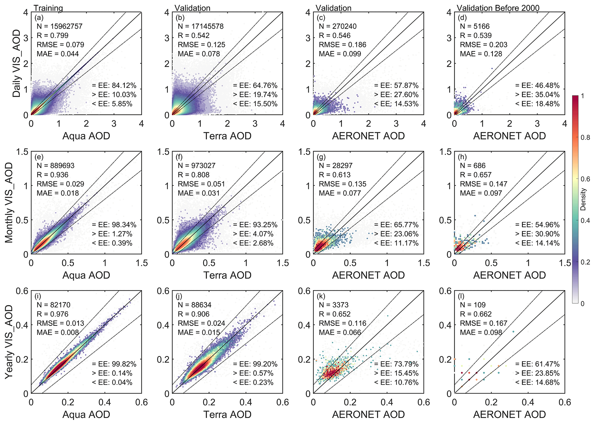
Figure 6 Scatter density plots between predicted AOD (VIS_AOD) and Aqua MODIS AOD, Terra MODIS AOD, AERONET AOD, and AERONET AOD before 2000 at the daily (a–d), monthly (e–h), and yearly (g–i) scale. The solid black line represents the 1:1 line and the dashed lines represent expected error (EE) envelopes. The sample size (N), correlation coefficient (R), mean absolute error (MAE), and root mean square error (RMSE) are given. “= EE”, “> EE”, and “< EE” represent the percentage (%) of retrievals falling within, above, and below the EE, respectively. Note that Aqua AOD is not an independent validation dataset for the predicted results, whereas Terra and AERONET AOD are independent validation datasets.

Figure 6 shows the scatter density plots and the EEs between VIS_AOD and Aqua AOD, Terra AOD, and AERONET AOD. Aqua AOD is not an independent validation dataset, while Terra and AERONET AOD are independent validation datasets. For the daily scale, the R, RMSE, and MAE between VIS_AOD and Aqua AOD (15 962 757 data pairs) are 0.799, 0.079, and 0.044, respectively. The percentage of sample points falling within the EE envelopes is 84.12 % at the global scale (Fig. 6a). The R value between VIS_AOD and Terra AOD (17 145 578 data pairs) is 0.542, with an RMSE of 0.125 and an MAE of 0.078. The percentage of sample points falling within the EE envelopes is 64.76 % (Fig. 6b). The R value between VIS_AOD and AERONET AOD (270 240 data pairs) at 395 sites is 0.546, with an RMSE of 0.186 and an MAE of 0.099. The percentage of sample points falling within the EE envelopes is 57.87 % (Fig. 6c).

For the monthly and yearly scales, RMSE and MAE show a significant decrease between VIS_AOD and Aqua, Terra, and AERONET AOD, with the R values and percentages falling within the EE showing a significant increase (Fig. 6e–g and i–k). The monthly RMSE values are 0.029, 0.051, and 0.135; the monthly MAE values are 0.018, 0.031, and 0.077; and the monthly R values are 0.936, 0.808, and 0.613, respectively. The percentages falling within the EE envelopes are 98.34 %, 93.25 %, and 65.77 %. The RMSE values at the yearly scale are 0.013, 0.024, and 0.116; the MAE values are 0.008, 0.015, and 0.066; and the R values are 0.976, 0.906, and 0.652, respectively. The percentages falling within the EE envelopes are 99.82 %, 99.20 %, and 73.79 %, respectively. The percentage falling within the EE envelopes when compared with AERONET is smaller than when compared against Terra, which may be related to the elevation of the AERONET sites, the distance between the AERONET and meteorological stations, and the observed time. The results highlighted above demonstrate a clear improvement in performance at the monthly and yearly scales compared with the daily scale.

To further examine the predictive capability of historical data, we compare the VIS_AOD with AERONET AOD before 2000, as shown in Fig. 6d, h, and l. We match 43 AERONET sites, with a total of 5166 daily records. The result indicates that the daily-scale R is close to the value after 2000 (Fig. 6c), with almost 50 % falling within the EE envelopes. The monthly and annual correlation coefficients are even higher, with 55 % falling within the EE envelopes. Despite the small sample size, the model still demonstrates excellent predictive ability. Compared with AERONET (an independent validation dataset), the performance of VIS_AOD is almost unchanged before and after 2000.

Figure 7 Scatter density plots between AERONET AOD and the predicted AOD (VIS_AOD) and MERRA-2 AOD before and after 2000 at the monthly scale. The solid black line represents the 1:1 line and the dashed lines represent the expected error (EE) envelopes. The sample size (N), correlation coefficient (R), mean absolute error (MAE), and root mean square error (RMSE) are given. “= EE”, “> EE”, and “< EE” represent the percentage (%) of retrievals falling within, above, and below the EE, respectively.

We also compare the VIS_AOD with the MERRA-2 reanalysis AOD at the monthly scale, as shown in Fig. 7. The correlation coefficient between MERRA-2 and AERONET is 0.655 before 2000, slightly lower than the correlation coefficient (0.657) between VIS_AOD and AERONET. The correlation coefficient between MERRA-2 and AERONET is 0.829 after 2000, significantly higher than that before 2000, while the correlation coefficient between VIS_AOD and AERONET is 0.613. This suggests that VIS_AOD and MERRA-2 AOD have similar accuracy before 2000. The correlation coefficient of MERRA-2 after 2000 is higher and performs even better than MODIS retrievals (as shown in Fig. 5) when evaluated at AERONET sites. However, before 2000, the correlation coefficient of MERRA-2 and AERONET as well as the RMSE and MAE all show significant changes and differences in consistency. The higher correlation between MERRA-2 and AERONET AOD is partly because MERRA-2 has assimilated AERONET AOD observations (Gelaro et al., 2017). Compared with AERONET, VIS_AOD and Aqua and Terra MODIS have a similar correlation coefficient. The correlation coefficient of VIS_AOD before 2000 is even higher than after 2000, and the changes in RMSE and MAE are not significant. This indicates the good consistency of VIS_AOD. In conclusion, the predicted results have good consistency with AERONET AOD and Terra AOD at the daily scale. There is a significant improvement in the monthly and annual results. The model shows good predictive capabilities before and after 2000, highlighting the stable accuracy of VIS_AOD.

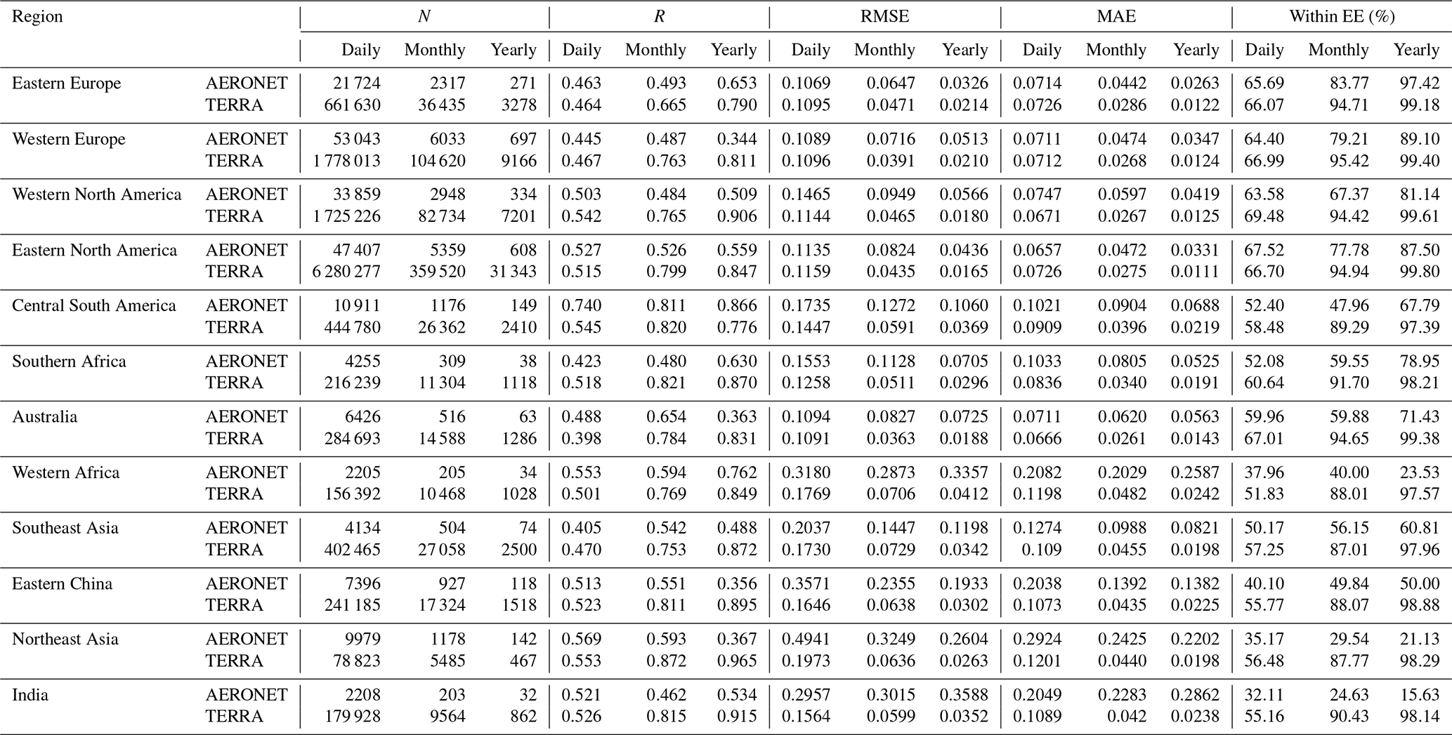
Table 1 Evaluation metrics for the relationships between visibility-derived AOD and AERONET AOD and Terra AOD for each region.

3.3.2 Validation over regions

Aerosol loading exhibits spatial variability. Evaluation metrics for the relationships between visibility-derived AOD and AERONET AOD and Terra AOD for each region are listed in Table 1.

In Europe and North America, the results are similar to those of Terra and AERONET, with a large number of data pairs, greater than 10⁵ (AERONET) and greater than 10⁷, except for Eastern Europe (Terra) at the daily scale. Approximately 63 %–70 % data pairs fall within the EE envelopes. The RMSE is approximately 0.11, except for Western North America (∼ 0.15); the MAE is approximately 0.07 and the correlation coefficient is between 0.44 and 0.54.

In Central South America, southern Africa, and Australia, the data pairs are about 10^3–4 (AERONET) and 10⁶ (Terra) at the daily scale; 52 %–60 % fall within the EE envelopes compared with AERONET and 58 %–67 % compared with Terra. The RMSE is 0.03–0.05 compared with Terra and 0.11–0.17 compared with AERONET. The correlation coefficient ranges from 0.40 to 0.74, with the highest correlation coefficient in South America at 0.74.

In Asia, India, and Western Africa, the data pairs are only approximately 10⁴ (AERONET); 32 %–50 % fall within the EE envelopes compared with AERONET. The RMSE value ranges from 0.20 to 0.50, and the MAE ranges from 0.11 to 0.36. Compared with Terra AOD, 51 %–58 % of data pairs fall within the EE envelopes; the RMSE is around 0.16, and the MAE is around 0.11. Compared with AERONET, in these high aerosol loading regions, RMSE and MAE increase, and the percentages falling within the EE envelopes decrease, but the correlation coefficients do not significantly decrease.

Compared with Terra AOD, 55 %–67 % of data fall within the EE envelopes at the daily scale, 87 %–96 % at the monthly scale, and over 97 % at the yearly scale. Compared with AERONET AOD, 32 %–68 % of data fall within the EE envelopes at the daily scale, 24 %–84 % at the monthly scale, and 15 %–97 % at the yearly scale. At both the monthly and yearly scales, all metrics have shown a significant increase in performance when compared with Terra. However, compared with AERONET, not all metrics increase in some regions due to limited data pairs, such as in Western Africa, Northeast Asia, and India, which may be due to the spatial differences between AERONET sites and meteorological stations.

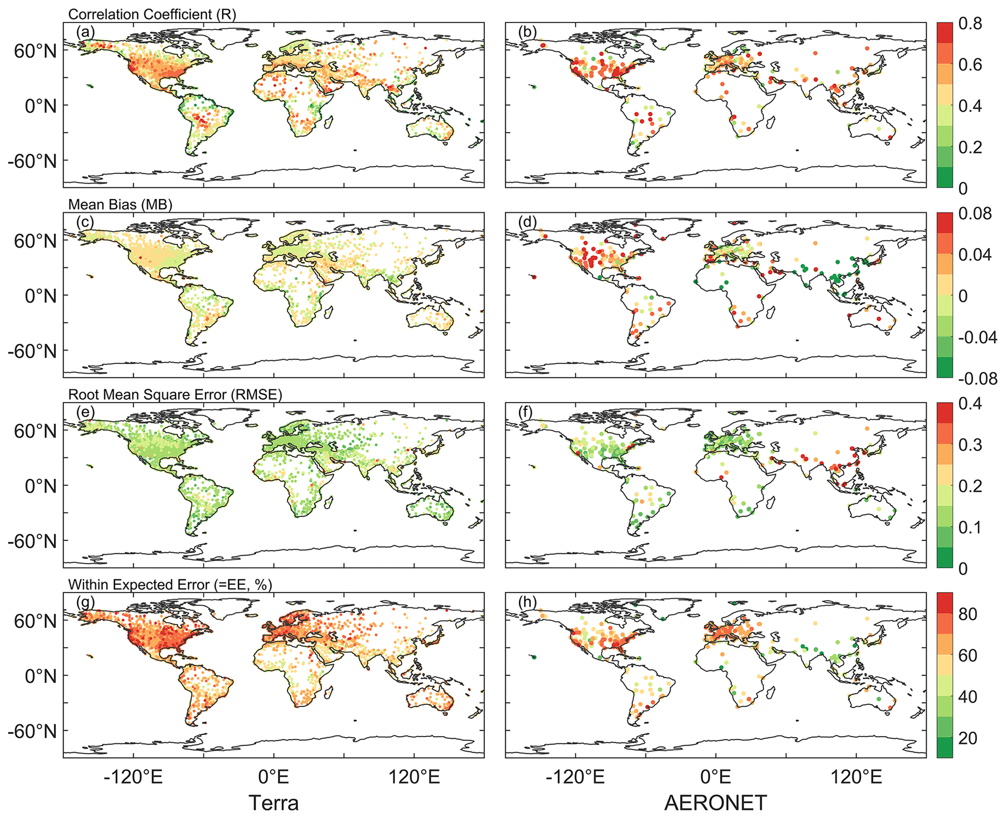
Figure 8 Validation of VIS_AOD against Terra and AERONET AOD at each site: (a, b) correlation (R), (c, d) mean bias (MB), (e, f) root mean square error (RMSE), and (g, h) percentage (%) of VIS_AOD within the expected error envelopes.

3.3.3 Validation at the site scale

Sites, especially AERONET, are not completely uniform around the world or in any region, and different stations have different sample sizes, which may lead to some uncertainty. Therefore, further analysis is conducted on the spatial distribution of different evaluation metrics. Figure 8 shows the validation and comparison of daily VIS_AOD against Terra and AERONET AOD at the site scale.

Compared with Terra daily AOD, the R value of 67 % of the stations is greater than 0.40, the mean bias of 83 % of the stations is less than 0.01, the RMSE of 85 % of the stations is less than 0.15, and the percentage falling within the EE is greater than 60 %. More than 85 % of the stations falling within the EE is greater than 60 % in Europe, North America, and Oceania, while 40 %–60 % in South America, Africa, and Asia. The percentage of expected error is low in Southeast Asia and Central Africa, with some underestimation. Over 60 % of stations in Africa, Asia, North America, and Europe have a correlation coefficient greater than 0.40. The regions with a lower correlation are the coastal regions of South America, Eastern Africa, Western Australia, Northeastern North America, and Northern Europe. Over 90 % of stations in Europe, North America, and Oceania have an RMSE less than 0.15. Regions with high RMSE values are Western North America, Asia, Central South America, and Central Africa.

Compared with AERONET daily AOD, the R value of 74 % of the stations is greater than 0.40, and the spatial distribution is similar to the Terra daily AOD. The mean bias in 44 % of the stations is less than 0.01, the RMSE of 68 % of the stations is less than 0.15, and the percentage falling within the EE of 53 % of the stations is greater than 60 %. More than 70 % of sites have a correlation coefficient greater than 0.40 in Africa, Asia, Europe, and North America. More than 57 % of sites have an expected error percentage of over 60 % in Europe, North America, and Oceania, except for Asia. Over 72 % of sites have an RMSE less than 0.15. Except for Oceania and South America, over 71 % of sites in other regions have MAE values less than 0.01. Almost all sites in Asia show a negative bias, with a significant underestimation. However, there is a significant overestimation in Western North America and Western Australia. The percentages of most sites in Asia falling within the expected error envelopes are less than 50 %. High RMSE values are found in areas of high emission and dust, such as Asia, India, and Africa.

The validation and comparison at the site scale show a limitation similar to the MODIS DT algorithm. In areas with high vegetation coverage, the AOD from visibility data is better than that in bright areas. Although the correlation coefficients are high in high aerosol loading areas (Central South America, Western Africa, India, Eastern China, Northeast Asia), there are significant differences in these areas with high RMSE values. As shown in Fig. 6, some stations located in dusty and urban areas show overestimations or underestimations. Studies have shown that there is a significant uncertainty in the MODIS retrievals in these regions, and the challenges of inversion algorithms are significant with bright surfaces (desert and snow-covered areas) and urban surfaces of densely populated complex structures (Chu et al., 2002; Remer et al., 2005; Levy et al., 2010; Wei et al., 2019, 2020). In India, the elevation difference between the AERONET site and the meteorological station reached 0.7 km, which may be a factor affecting the validation, as aerosol varies greatly with altitude. In Eastern China, the complex urban surface, emission sources, and observations in different locations (AERONET site and meteorological station) may be the reasons for the underestimation. At the same time, visibility stations in desert areas are sparse, and the spatial variability of dust aerosols is large, which also increases the difficulty in estimating VIS_AOD.

3.3.4 Discussion and uncertainty analysis

Atmospheric visibility is a surface physical quantity, while AOD is a column-integrated physical quantity. We have linked the two variables using machine a learning method, which partially compensates for the scarcity of AOD data. However, we have to face some limitations. Although the boundary layer height is considered, it is not sufficient. Pollutants such as smoke from biomass burning, dust, volcanic ash, and gas–aerosol conversion of sulfur dioxide to sulfate aerosols in the upper and lower troposphere can undergo long-range aerosol transport under the influence of circulation. The pollution transport and aerosol conversion processes above the boundary layer are still significant and cannot be ignored (Eck et al., 2023). Compared with surface visibility, bias occurs when the aerosol layer rises and affects AERONET measurements and MODIS retrievals; therefore, it should be considered when using these data. If there are sufficient historical vertical aerosol measurements with high temporal and spatial resolution, the results of these data would be greatly improved. Although some studies use aerosol profiles from pollution transport models or assumed profiles as substitutes for observed profiles (Li et al., 2020; Zhang et al., 2020), the biases introduced by these non-observed profiles are still significant.

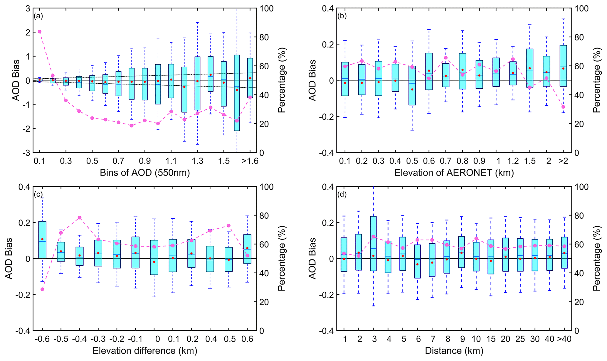
Figure 9 Box plots of AOD bias and the percentage of data falling within the EE envelopes (curves): (a) AERONET AOD levels, (b) elevation of AERONET sites, (c) elevation difference between meteorological stations and AERONET sites, and (d) distance (km) between meteorological stations and AERONET sites. The horizontal black line represents the zero bias. For each box, the upper, lower, and middle horizontal lines and the whiskers represent the AOD bias 75th and 25th percentiles, median, and 1.5 times the interquartile difference, respectively. The solid black lines represent the EE envelopes (± (0.05 + 0.15 ⋅ AOD_AERONET)). There is no site with a difference of +0.3 km (x-axis label without 0.3) in (c).

In machine learning, we use MODIS Aqua AOD as the target value for the model because the validation results for the MODIS C6.1 product have a correlation coefficient of 0.9 or higher with AERONET AOD at the daily scale (Wei et al., 2019, 2020). Compared with AERONET, MODIS AOD provides more sample data with a high global coverage. However, apart from modeling errors, the systematic biases and uncertainties of MODIS Aqua AOD cannot be ignored (Levy et al., 2013, 2018; Wei et al., 2019). Averaging over time scales can reduce representation errors effectively, while emission sources and orography can increase representation errors (Schutgens et al., 2017). Therefore, the strong correlation at monthly and annual scales indicates a substantial reduction in errors. This is also one of the reasons why this dataset shows a stronger correlation with Terra AOD and a weaker correlation with AERONET in the validation.

The spatial matching between meteorological stations and AERONET sites may cause some biases. AERONET sites are usually not co-located with meteorological stations in terms of elevation and horizontal distance, and this is another reason for the weak correlation between VIS_AOD and AERONET AOD. The meteorological stations are located at airports. Different horizontal distances may result in meteorological stations and AERONET sites being located on different surfaces (such as urban, forest, or mountainous areas). Differences in site elevation significantly impact the relationship between AOD and the measured visibility. When the AERONET site is at a higher elevation than the meteorological station, there may be fewer measurements of aerosols over the sea at the AERONET site.

Different pollution levels and station elevations affect the AOD derived from visibility. The elevation difference and the distance between meteorological stations and AERONET sites also have an impact on the validation results. Therefore, the error and performance of different AERONET AOD values, station elevations, and distances are analyzed.

As the AOD increases, the variability of bias also increases in Fig. 9a. Almost all mean bias values are within the EE envelope, except for 1.1–1.2 and 1.5–1.6. The average bias is 0.015 (AOD < 0.1), with 83 % of the data within the EE envelopes. The mean bias is −0.0011 (AOD, 0.1–0.2), with 54 % within the EE envelopes. The mean bias is negative (AOD, 0.3–1.0), with 20 %–40 % falling within the EE envelopes. There is a positive bias (AOD at 1.1, 1.4, and > 1.6), and there is a negative bias at 1.2–1.3 and 1.5–1.6. These results indicate that as the pollution level increases, the negative mean bias becomes significant and the underestimation increases.

The contribution of aerosols near the ground to the column aerosol loading is significant. The elevation of the site affects the measurement of column aerosol loading in Fig. 9b. There is a negative bias at low elevation (≤ 0.5 km), with 60 %–64 % falling within the EE envelopes, and a positive bias at high elevation (0.5–1.2 km), with 50 %–65 % falling within the EE envelopes. The percentage significantly decreases (> 1.2 km) and the average bias increases. Therefore, the elevation of AERONET sites will cause bias in the validation, and the uncertainty greatly increases at high elevation.

Due to the elevation difference between the meteorological station and the AERONET site in the vertical direction, the uncertainty caused by elevation differences at the site is analyzed in Fig. 9c. When the elevation difference is negative (the elevation of the meteorological station is lower than that of the AERONET site), there is a significant positive bias. When the difference is positive, the mean bias approaches 0 or is positive. The percentage is greater than 60 % (−0.5 to 0.5 km). The positive mean bias is greater than the negative mean bias, and the uncertainty greatly increases when the elevation of the meteorological stations is lower than that of the AERONET sites. This indicates that the contribution of the near-surface aerosol to the column aerosol loading is significant and cannot be ignored.

The spatial variability of aerosols is significant. Meteorological stations and AERONET sites are not co-located, resulting in a certain distance in spatial matching. In this study, the upper limit in distance is 0.5°. Figure 9d shows the error of the distance between stations, where the degree is converted to the distance at WGS84 coordinates. The bias does not change significantly with increasing distance. The average bias is around 0, with the maximum positive mean bias (0.0322) at a distance of 2 km and the maximum negative mean deviation (−0.0323) at 6 km. The median is almost positive, except at 5 and 6 km. The percentage falling within the EE envelopes is over 50 %, with the maximum percentage (66 %) at 3km and the minimum (62 %) at 2 km.

Figure 10 Map of annual and seasonal mean AOD (left) and global and regional mean time series from 1980 to 2021 (right). Global land (circle), Northern Hemisphere (NH) (triangle), and Southern Hemisphere (SH) (square) annual and seasonal AOD. The symbol ${}^{\ast \ast }$ indicates the trend passed the test at a significance level of 0.01. The symbol ^∗ indicates the trend passed the test at a significance level of 0.05. DJF represents December and the next January and February. MAM represents March, April, and May. JJA represents June, July, and August. SON represents September, October, and November.

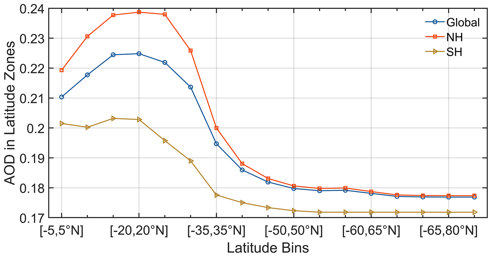
Figure 11 Global land (blue), Northern Hemisphere (red), and Southern Hemisphere (yellow) multi-year average VIS_AOD from 1980 to 2021 in different latitude zones. The latitude range is from −65 to 85° N, with a bin of 5°.

3.4 Interannual variability and trend in visibility-derived AOD over global land

The multi-year average AOD from 1980 to 2021 over land is 0.177, as shown in Fig. 10a. The average is 0.178 in the Northern Hemisphere (NH, 4532 stations) and 0.174 in the Southern Hemisphere (SH, 500 stations). Due to the influence of geography, atmospheric circulation, population, and emissions, the AOD varies at different latitudes. Figure 11 illustrates the multi-year average AOD at different latitude ranges from 1980 to 2021. The AOD value in the NH is higher than that over land and higher than that in the SH. Within −20 to 20° N, the average AOD reaches its maximum (0.225), and the maximum AOD in the NH is 0.239 (0–20° N). The highest AOD in the SH is 0.203 (−15 to 0° N). The average AOD rapidly decreases from −15 to −35° N in the SH and from 20 to 50° N in the NH.

There are many regions of high AOD values in the NH with the distribution of high population density. Approximately seven-eighths of the global population resides in the NH, with 50 % concentrated at 20–40° N (Kummu et al., 2016), indicating a significant impact of human activities on aerosols. The highest AOD values are observed near 17° N, including the Sahara Desert, Arabian Peninsula, and India, suggesting that in addition to anthropogenic sources, deserts also play a crucial role in aerosol emissions. Lower AOD regions in the SH are from 25 to 60° S, encompassing Australia, southern Africa, and southern South America, indicating lower aerosol burdens in these areas. Additionally, North America also exhibits low aerosol loading. Chin et al. (2014) analyzed the AOD over land from 1980 to 2009 with the Goddard Chemistry Aerosol Radiation and Transport model, which is similar to the visibility-derived AOD. The spatial distribution is consistent with the satellite results (Remer et al., 2008; Hsu et al., 2012, 2017; Tian et al., 2023). The AOD and extinction coefficients retrieved from visibility show a similar distribution at the global scale, with a correlation coefficient of nearly 0.6 (Mahowald et al., 2007). Similar global (Husar et al., 2000; Wang et al., 2009) and regional (Koelemeijer et al., 2006; Wu et al., 2014; Boers et al., 2015; Zhang et al., 2017, 2020) spatial distributions have been reported.

AOD loadings exhibit significant seasonal variations worldwide, particularly over land. In this study, a year is divided into four parts – December–January–February (DJF), March–April–May (MAM), June–July–August (JJA), and September–October–November (SON) – corresponding to winter (summer), spring (autumn), summer (winter), and autumn (spring) in the NH (SH), respectively. Figure 10b–e also depict the spatial distribution of seasonal average AOD over land from 1980 to 2021. The global AOD in DJF, MAM, JJA, and SON is 0.161, 0.176, 0.204, and 0.164, respectively. The standard bias of AOD in JJA and DJF is greater than that in DJF and SON. AOD exhibits seasonal changes, with the highest in JJA followed by DJF, MAM, and SON.

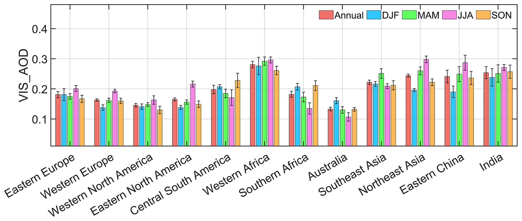
Figure 12 Annual and seasonal mean AOD in 12 regions (Eastern Europe, Western Europe, Western North America, Eastern North America, Central South America, Western Africa, Southern Africa, Australia, Southeast Asia, Northeast Asia, Eastern China, and India) during the period 1980–2021.

In the NH, the AOD ranking is summer (0.210) > spring (0.176) > autumn (0.163) > winter (0.160). In the SH, the AOD ranking from high to low in season is spring (0.188) > summer (0.184) > autumn (0.164) > winter (0.152). The highest AOD is observed during JJA in the NH, while in the SH, the peak occurs during SON. The high AOD value is significantly associated with the growth in hygroscopic particles and the photochemical reaction of aerosol precursors under higher relative humidity in Asia (JJA) (Remer et al., 2008) and Europe, such as in Russia (JJA), and with biomass burning in South America (SON), southern Africa (SON), and Indonesia (SON) (Ivanova et al., 2010; Krylov et al., 2014). On the other hand, the lowest global AOD values are observed during winter, which may be attributed to the atmospheric circulation systems (Li et al., 2016; Zhao et al., 2019).

The temporal variations in AOD have also been of great interest due to the significant relationship between aerosols and climate change. Figure 10f shows the trends in annual average AOD (${}^{\ast \ast }$ represents passing the significance test, p < 0.01) over the global land area, the SH, and the NH during 1980–2021. The global land, NH, and SH demonstrate a decreasing trend in AOD, with values of −0.0029 per 10 years, −0.0030 per 10 years, and −0.0021 per 10 years, respectively – all passing the significance test. The declining trend is much greater in the NH than in the SH.

The seasonal trends in AOD during 1980–2021 at the global and hemispheric scales are shown in Fig. 10g–j. There is a decreasing trend over land in DJF, JJA, and SON and an increasing trend in MAM. The largest declining trend is observed in SON (−0.0055 per 10 years). In the NH, the trends are −0.0044 per 10 years (DJF), 0.0016 per 10 years (MAM), −0.0024 per 10 years (JJA), and −0.0064 per 10 years (SON). In the SH, the trends are 0.0022 per 10 years (DJF), −0.0044 per 10 years (MAM), −0.0064 per 10 years (JJA), and 0.0033 per 10 years (SON). The largest declining trend is in SON in the NH and in JJA in the SH. However, the trends are positive in MAM in the NH and in DJF and SON in the SH.

3.5 Interannual variability and trend in visibility-derived AOD over regions

The distribution of AOD over global land exhibits significant spatial heterogeneity. Large variations in aerosol concentrations exist among different regions, leading to a non-uniform spatial distribution of AOD globally. Accurately assessing the long-term trends in aerosol loading is key for quantifying aerosol climate change and it is crucial for evaluating the effectiveness of measurements implemented to improve regional air quality and reduce anthropogenic aerosol emissions. Therefore, we select 12 representative regions to analyze the variability and trend in AOD which are influenced by various aerosol sources (Wang et al., 2009; Hsu et al., 2012; Chin et al., 2014), such as desert, industry, anthropogenic emissions, and biomass burning emissions, which cover the most land and are densely populated regions (Kummu et al., 2016). These representative regions are Eastern Europe, Western Europe, Western North America, Eastern North America, Central South America, Western Africa, Southern Africa, Australia, Southeast Asia, Northeast Asia, Eastern China, and India, as shown in Fig. 1.

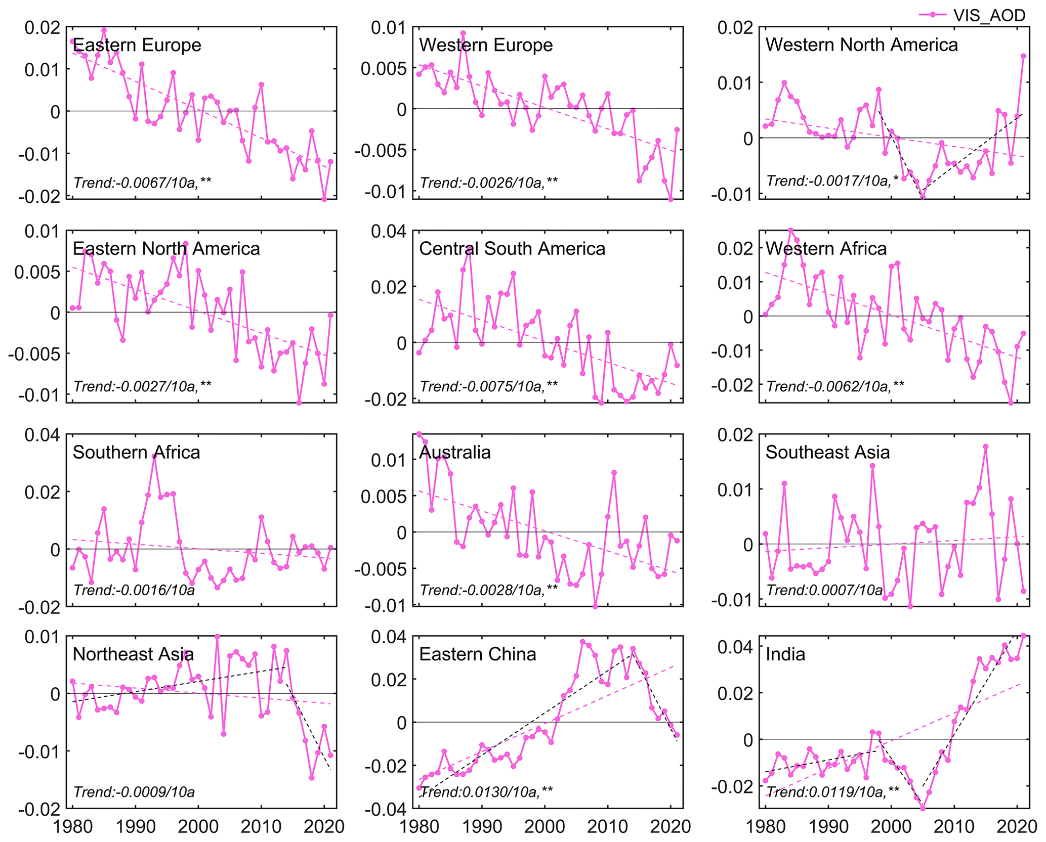
Figure 13 Annual anomaly of VIS_AOD from 1980 to 2021 in 12 regions (Eastern Europe, Western Europe, Western North America, Eastern North America, Central South America, Western Africa, Southern Africa, Australia, Southeast Asia, Northeast Asia, Eastern China, and India). The dotted line is the trend line.

Figure 14 Seasonal mean VIS_AOD from 1980 to 2021 in 12 regions (Eastern Europe, Western Europe, Western North America, Eastern North America, Central South America, Western Africa, Southern Africa, Australia, Southeast Asia, Northeast Asia, Eastern China, and India). The dotted line is the trend line.

The multi-year average and seasonal average AOD (Fig. 12), the trends in the annual average of monthly anomalies (Fig. 13), and the seasonal trends (Fig. 14) are analyzed in 12 regions from 1980 to 2021.

The regions with a high aerosol level (AOD > 0.2) are in Western Africa, Southeast and Northeast Asia, Eastern China, and India. The AOD values range from 0.15 to 0.2 in Eastern Europe, Western Europe, Eastern North America, Central South America, and Southern Africa. The AOD values are less than 0.15 in Western North America and Australia.

Europe is an industrial region with low aerosol loading, and the multi-year average AOD in Eastern Europe (0.181) is higher than that in Western Europe (0.163) during 1980–2021. Eastern Europe shows a greater downward trend in AOD (−0.0067 per 10 years) compared with Western Europe (−0.0026 per 10 years). The highest AOD is observed in JJA, i.e., the dry period when solar irradiation and boundary layer height increase, with AOD values of 0.201 in Eastern Europe and 0.162 in Western Europe, which could be due to increases in secondary aerosols, biomass burning, and dust transport from the Sahara (Mehta et al., 2016). However, there are seasonal variations. In Eastern Europe, the seasonal AOD ranking from high to low is JJA (0.201) > DJF (0.181) > MAM (0.175) > SON (0.161), while in Western Europe, it is JJA (0.193) > MAM (0.162) > SON (0.160) > DJF (0.138). The differences among seasons are larger in Western Europe. AOD in Eastern Europe shows declining trends (p < 0.01) in all seasons, and the largest declining trend is in DJF (−0.0096 per 10 years). In Western Europe, the AOD in DJF, JJA, and SON exhibits declining trends, while the AOD in MAM shows a significant increasing trend (0.0019 per 10 years). There is an increasing trend in MAM in both Western and Eastern Europe from 1995 to 2005, with Western Europe showing a greater increasing trend. However, after 2005, the declining rates accelerate in each season. Studies have shown the downward trend in Europe is attributed to the reduction in biomass burning, anthropogenic aerosols, and aerosol precursors (such as sulfur dioxide) (Wang et al., 2009; Chin et al., 2014; Mortier et al., 2020).

North America is also an industrial region with low aerosol loading. The average AOD values in Eastern and Western North America during 1980–2021 are 0.165 and 0.146, respectively, with the Eastern region being higher than the western region by 0.019. From 1980 to 2021, both Eastern (−0.0027 per 10 years) and Western North America (−0.0017 per 10 years) show a downward trend. The AOD values in DJF, MAM, JJA, and SON in Western North America are 0.141, 0.148, 0.163, and 0.130, respectively, and in Eastern North America they are 0.138, 0.156, 0.216, and 0.149. Specifically, the trends in the Western and Eastern regions increase during MAM and decrease during other seasons. In the western region, the trend increases after 2005, while in the eastern region, there is no increasing trend. The increasing trend may be due to low rainfall and increased wildfire activities (Yoon et al., 2014). The decreasing trend in Eastern North America is related to the reduction in sulfate and organic aerosols as well as the decrease in anthropogenic emissions caused by environmental regulations (Mehta et al., 2016).

Central South America is a relatively high aerosol loading region, sourced from biomass burning, especially in SON (Remer et al., 2008; Mehta et al., 2016), with a multi-year average AOD of 0.198. There is a downward trend (−0.0075 per 10 years) from 1980 to 2021. The trend is slightly lower than the trend (−0.0090 per 10 years) from 1998 to 2010 (Hsu et al., 2012), and the trend decreases from 1980 to 2006 (Streets et al., 2009) and from 2001 to 2014 (Mehta et al., 2016). The AOD values in DJF (0.207) and SON (0.228) are higher compared with the values in MAM (0.185) and JJA (0.171), and the larger declining trends are observed in MAM (−0.0100 per 10 years) and JJA (−0.0150 per 10 years). The result indicates that although AOD has decreased overall, the aerosol loading is still high, which is caused by deforestation and biomass burning (Mehta et al., 2016).

Africa is a high aerosol loading region. In Western Africa, the multi-year average AOD is 0.281, with a decreasing trend (−0.0062 per 10 years) from 1980 to 2021. The world's largest desert (the Sahara) is in Western Africa, with much dust emission. The AOD values in JJA (0.296), MAM (0.292), DJF (0.276), and SON (0.261) are over 0.26. The trends in DJF (−0.0145 per 10 years), MAM (−0.0015 per 10 years), JJA (−0.0019 per 10 years), and SON (−0.0078 per 10 years) are decreasing. For southern Africa, the multi-year average AOD is 0.182, lower than that of Western Africa, with a decreasing trend (−0.0016 per 10 years). The results of AERONET observations and simulation also show a decreasing trend (Chin et al., 2014). The AOD values range from 0.12 to 0.20 during 2000–2009 dominated by fine particle matter from industrial pollution from biomass and fossil fuel combustion (Hersey et al., 2015). The average AOD values in DJF, MAM, JJA, and SON are 0.207, 0.173, 0.135, and 0.21, with trends of 0.0044 per 10 years, −0.0089 per 10 years, −0.0089 per 10 years, and 0.0063 per 10 years, respectively.

Australia is a region with a low aerosol loading. The multi-year average AOD is 0.133 during 1980–2021. The AOD ranges from 0.05 to 0.15 from AERONET during 2000–2021, and dust and biomass burning are important contributors to the aerosol loading (Yang et al., 2021a). There is a downward trend in AOD (−0.0028 per 10 years), which may be related to a decrease in dust and biomass burning (Yoon et al., 2016; Yang et al., 2021a). In addition, a study has shown that the forest area in Australia has increased sharply since 2000 (Giglio et al., 2013), surpassing the forest fire area of the past 14 years. The seasonal average AOD in MAM, JJA, SON, and DJF is 0.130, 0.107, 0.132, and 0.161, respectively. The AOD in JJA is the lowest in all seasons and in all regions. The trends in DJF and SON are increasing, and the trends in MAM and JJA are decreasing. Ground-based observations and satellite retrievals indicate that wildfires, biomass burning, and sandstorms lead to high AOD in DJF and SON. The low AOD in MAM and JJA is due to a decrease in the frequency of sandstorms and wildfires and an increase in precipitation (Gras et al., 1999; Yang et al., 2021a; Yang et al., 2021b).

Asia is also a high aerosol loading area with various sources. In Southeast Asia, the multi-year average AOD is 0.222 during 1980–2021, with a downward trend in AOD (0.0007 per 10 years). It is also a biomass-burning area. The seasonal average AOD ranking is MAM (0.251) > DJF (0.216) > SON (0.212) > JJA (0.209). There is a decreasing trend in DJF (−0.0018 per 10 years) and an increasing trend in MAM (0.0330 per 10 years), JJA (0.0008 per 10 years), and SON (0.0006 per 10 years). However, the trends are insignificant. Southeast Asia has no clear long-term trend in estimated AOD or ground-based observations (Streets et al., 2009). In Northeast Asia, the multi-year average AOD is 0.244 during 1980–2021, with a trend of −0.0009 per 10 years. The trend increases (0.0018 per 10 years) during 1980–2014 and decreases (−0.0213 per 10 years) during 2014–2021. The seasonal AOD values are 0.196 in DJF, 0.260 in MAM, 0.287 in JJA, and 0.236 in SON. The high aerosol level is related to dust and aerosol transportation in East Asia. There is an increasing trend in DJF (0.0016 per 10 years) and MAM (0.0062 per 10 years) and a decreasing trend in JJA (−0.0043 per 10 years) and SON (−0.0070 per 10 years). In Eastern China, the multi-year average AOD is 0.241, with an increasing trend (0.0130 per 10 years). The trend is 0.0196 per 10 years from 1980 to 2014 and −0.0572 per 10 years from 2014 to 2021. The seasonal ranking of AOD from high to low is JJA (0.287), MAM (0.249), SON (0.236), and DJF (0.216). The AOD trends in DJF (0.0133 per 10 years), MAM (0.0179 per 10 years), JJA (0.0107 per 10 years), and SON (0.0105 per 10 years) are all positive. The trend can be divided into three stages: 1980–2005, 2006–2013, and 2014–2021. In the first stage, AOD values increase steadily. In the second stage, AOD values maintain a high level. In the third stage, the AOD values experience a rapid decline, reaching the 1980s level by 2021. The increasing trend in AOD before 2006 may be due to the significant increase in industrial activity; after 2013 the significant decrease is closely related to the implementation of air-quality-related laws and regulations, along with adjustments in the energy structure (Hu et al., 2018; Cherian and Quaas, 2020).

India is a high aerosol loading area. The multi-year average AOD is 0.254, with an increasing trend (0.0119 per 10 years) from 1980 to 2021. Dust and biomass burning have an influence on AOD. There are three stages in the trend: 1980–1997 (0.0050 per 10 years), 1997–2005 (−0.0393 per 10 years), and 2005–2021 (0.0446 per 10 years). The seasonal average AOD values are 0.238 in DJF, 0.251 in MAM, 0.271 in JJA, and 0.257 in SON. The largest AOD is in JJA. In winter and autumn, the aerosol level is affected by biomass burning, and in spring and summer, it is also affected by dust transported from the Sahara during the monsoon period (Remer et al., 2008). The trends in DJF (0.0186 per 10 years), MAM (0.0143 per 10 years), JJA (0.0012 per 10 years), and SON (0.0129 per 10 years) are positive.

The above results have supplemented the existing estimates of long-term AOD variability and trend over land. The AOD level at the regional scale shows significant differences from 1980 to 2021, which is strongly related to the aerosol emission source types, transportation, and implementation of laws and regulations for pollution control.

4 Data availability

We provide the daily visibility-derived AOD data at 5032 stations over global land from 1959 to 2021, which are available at the National Tibetan Plateau/Third Pole Environment Data Center, https://doi.org/10.11888/Atmos.tpdc.300822 (Hao et al., 2023). Due to the small number and sparse visibility stations prior to 1980, the global and regional analysis in this study is from 1980 to 2021. The following is a description of the AOD dataset.

The station-scale AOD files are in “Station_Daily_AOD_1959_2021.zip”. The station-scale AOD files can be directly opened by a text program (such as Notepad). Details on the station information are in the file “0A0A-Station_In Information.txt”. There are eight columns in each text file, separated by commas, and the column names are Datetime, TEMP (°), DEW (°), RH (%), WS (m s⁻¹), SLP (hPa), DRYVIS (km), and VIS_AOD (550 nm). The first column name is the date. The column “VIS_AOD (550 nm)” is the AOD at 550 nm. The second through seventh columns are temperature (unit: °), dew temperature (unit: °), relative humility (unit: %), wind speed (unit: m s⁻¹), sea level pressure (unit: hPa), and dry visibility (unit: km). More details are given in “0A0B-ReadMe.txt”.

5 Conclusions

In this study, we employ a machine learning method to derive daily AOD at 550 nm during 1959–2021 at 5032 land stations worldwide based on visibility, satellite retrieval, and related meteorological variables. In the model, Aqua MODIS AOD (550 nm) is set as the target and visibility and related meteorological variables are set as the predictor. The performance and predictive ability of the model are evaluated and validated against AERONET ground-based observations, Terra MODIS AOD, and MERRA-2 AOD. We provide a long-term daily AOD (550 nm) dataset at 5032 global land stations from 1959 to 2021. The dataset overcomes the shortcomings of AOD data in terms of time scale and spatial coverage over land. Finally, the variability and trend in AOD are analyzed at the global and regional scales for the past 42 years. Several key findings are established in this study, as follows:

1. Modeling evaluation. For all stations, the mean RMSE, MAE, and R of the model are 0.078, 0.044, and 0.75, respectively. The RMSE of 93 % of the stations is less than 0.110, the MAE of 91 % of the stations is less than 0.060, and the R of 88 % of the stations is greater than 0.70.

2. Model validation. For the daily scale, the R, RMSE, and MAE between VIS_AOD and Aqua AOD are 0.799, 0.079, and 0.044, respectively. The percentage of sample points falling within the EE envelopes is 84.12 %. The R between VIS_AOD and Terra AOD is 0.542, with an RMSE of 0.125 and an MAE of 0.078. The percentage of data falling within the EE envelopes is 64.76 %. The R between VIS_AOD and AERONET AOD is 0.546, with an RMSE of 0.186 and an MAE of 0.099. The percentage of sample points falling within the EE envelopes is 57.87 %. For the monthly and annual scales, RMSE and MAE show a significant decrease between VIS_AOD and Aqua, Terra, and AERONET AOD, and the R values and percentage of data falling within the EE envelopes show a significant increase. Compared with AERONET AOD and MERRA-2 AOD prior to 2000, the model has consistent predictive ability.

3. Error analysis. As the AOD value increases, the average bias increases. When the pollution level is low (AOD < 0.1), the average bias is 0.015, with 83 % of data falling within the EE envelopes. As the pollution level increases, the negative average bias becomes significant and the underestimation increases. The elevation of the AERONET site also causes a bias. At low elevation (≤ 0.5 km), there is a negative bias, with 60 %–64 % of the data falling within the EE envelopes. At high elevation (0.5–1.2 km), there is a positive bias, with 50 %–65 % of data falling within the EE envelopes. When the elevation difference is negative (the elevation of the meteorological station is lower than that of the AERONET site), there is a significant positive bias. When the difference is positive, the mean bias approaches 0 or is positive. The influence of distance between the meteorological station and the AERONET site on bias is not significant.

4. Global land AOD. The mean AOD from 1980 to 2021 is 0.177 over land, 0.178 in the NH, and 0.174 in the SH, with a trend of −0.0029 per 10 years, 0.0030 per 10 years, and −0.0021 per 10 years, respectively. The seasonal AOD rankings are JJA (0.204) > MAM (0.176) > SON (0.164) > DJF (0.161) over global land, JJA (0.210) > MAM (0.176) > SON (0.163) > DJF (0.160) in the NH, and SON (0.188) > DJF (0.184) > MAM (0.14) > JJA (0.152) in the SH. The largest decreasing trends are in SON in the NH (−0.0064 per 10 years) and in JJA in the SH (−0.0064 per 10 years). The increasing trends are in MAM in the NH and in DJF and SON in the SH.

5. Regional AOD. The high aerosol loading (AOD > 0.2) regions are Western Africa, Southeast and Northeast Asia, Eastern China, and India, with a trend of −0.0062 per 10 years, 0.0007 per 10 years, −0.0009 per 10 years, 0.0133 per 10 years, and 0.0119 per 10 years, respectively. However, the trends decrease in Eastern China (−0.0572 per 10 years) and Northeast Asia (−0.0213 per 10 years) after 2014, and the larger increasing trend is found after 2005 in India (0.0446 per 10 years). The moderate aerosol loading (AOD between 0.15 and 0.2) regions are Eastern Europe, Western Europe, Eastern North America, Central South America, and Southern Africa, with a trend of −0.0067 per 10 years, −0.0026 per 10 years, −0.0027 per 10 years, −0.0062 per 10 years, and −0.0016 per 10 years, respectively. The low aerosol loading (AOD < 0.15) regions are Western North America and Australia, with a trend of −0.0017 per 10 years and −0.0028 per 10 years. However, the trends in Southern Africa, Southeast Asia, and Northeast Asia are not significant.