the Creative Commons Attribution 4.0 License.
the Creative Commons Attribution 4.0 License.
 | 09 Jul 2024
A new repository of electrical resistivity tomography and ground-penetrating radar data from summer 2022 near Ny-Ålesund, Svalbard
Andrea Vergnano
Alberto Godio
Gerardo Romano
Luigi Capozzoli
Ilaria Baneschi
Marco Doveri
Alessandro Santilano
We present the geophysical data set acquired in summer 2022 close to Ny-Ålesund (western Svalbard, Brøggerhalvøya Peninsula, Norway) as part of the project ICEtoFLUX. The aim of the investigation is to characterize the role of groundwater flow through the active layer as well as through and/or below the permafrost. The data set is composed of electrical resistivity tomography (ERT) and ground-penetrating radar (GPR) surveys, which are well-known geophysical techniques for the characterization of glacial and hydrological processes and features. Overall, 18 ERT profiles and 10 GPR lines were acquired, for a total surveyed length of 9.3 km. The data have been organized in a consistent repository that includes both raw and processed (filtered) data. Some representative examples of 2D models of the subsurface are provided, that is, 2D sections of electrical resistivity (from ERT) and 2D radargrams (from GPR). The resistivity models revealed deep resistive structures, probably related to the heterogeneous permafrost, which are often interrupted by electrically conductive regions that may relate to aquifers and/or faults. The interpretation of these data can support the identification of the active layer, the occurrence of spatial variation in soil conditions at depth, and the presence of groundwater flow through the permafrost. To a large extent, the data set can provide new insight into the hydrological dynamics and polar and climate change studies of the Ny-Ålesund area. The data set is of major relevance because there are few geophysical data published about the Ny-Ålesund area. Moreover, these geophysical data can foster multidisciplinary scientific collaborations in the fields of hydrology, glaciology, climate, geology, and geomorphology, etc. The geophysical data are provided in a free repository and can be accessed at https://doi.org/10.5281/zenodo.10260056 (Pace et al., 2023).
- Article
(10721 KB) - Full-text XML
- BibTeX
- EndNote


The Earth's interior and its physical properties are imaged using quantitative methods. Geophysical measurements on the Earth's surface can reveal how the subsurface physical properties vary in space and possibly in time (Telford et al., 1990).
The Svalbard Archipelago (High Arctic Norway, see Fig. 1a) is believed to be representative of a typical Arctic critical environment (Dallmann, 2015). The location of the Svalbard Archipelago is ideal for observing the Arctic environment in general, from the perspectives of glaciology, geology, biodiversity, and climate change impact (Gevers et al., 2023). Climate change heavily affects the Arctic hydrologic dynamics, generating significant environmental modifications and potentially leading to the climatic feedback and warming amplification (Wadhams, 2017).
Ny-Ålesund is the northernmost settlement in the world (79° N), located in western Spitsbergen in the Svalbard Archipelago (see Fig. 1b). It serves as a scientific hub for the international research community, their equipment, and some essential logistical support (Paglia, 2020). Ny-Ålesund represents an outstanding natural laboratory for any topic of scientific research in the Arctic, being situated in the Kongsfjorden Fjord, where glaciers, rivers, coast, sea, atmosphere, animals, plants, and their interaction can be monitored (Gevers et al., 2023; Pedersen et al., 2022). From a geophysical point of view, the Svalbard Archipelago is interesting because of the presence of permafrost with a seasonal active layer, springs, aquifers, sea water, and old coal mines. Spatial heterogeneity in geophysical properties is expected due to the local lithology and structural framework as well as the geomorphologic features linked to the past movement of the glaciers (Orvin, 1934; Dallmann, 2015).
Ny-Ålesund is also an ideal place for hydrogeological studies, because 3 km from the settlement there is the Bayelva River catchment, where the entire water cycle from the glaciers to the sea can be studied within an area of a few squared kilometers (see Fig. 1c). In formerly glacierized watersheds, hydrologic processes are evolving, with new storage mechanisms and distribution of water resources, such as more persistent rivers and developed groundwater systems. Over the past few years, investigations on the Arctic freshwater increased, but broad knowledge about processes that govern water flow dynamics in High Arctic basins is still quite limited (Svendsen et al., 2002).
Applied geophysics can be of great help in unraveling the complexity of the water cycle and improving our knowledge about groundwater flow by means of non-destructive measurements from the surface (Hauck and Kneisel, 2008). Geophysical techniques, such as electrical resistivity tomography (ERT), ground-penetrating radar (GPR), passive and active seismic methods (Kula et al., 2018), and electromagnetic induction (EMI) methods (Kasprzak, 2020; Hill, 2020), have been used to survey the Arctic areas around the world, for example, to detect the heterogeneity in the permafrost, to monitor glacial and periglacial processes, or to understand the role of ice in hydrology (Hauck and Kneisel, 2008; Rossi et al., 2022). EMI methods have been adopted in the Svalbard Archipelago to characterize the geology (Beka et al., 2015, 2017b), possible geothermal applications (Beka et al., 2016), and CO2 storage (Beka et al., 2017a).
This paper focuses on the ERT and GPR methods for the following reasons. The ERT method has been successfully adopted in the Arctic environment because of its effectiveness in imaging the variation in the electrical resistivity values of aquifers, permafrost, and the active layer, both at lower and higher depth, depending on the chosen acquisition settings. The electrical resistivity values are typically high for permafrost and low for water-saturated soil, and therefore they can be easily distinguished. The GPR method is largely adopted for glaciological studies because the radar signal travels easily and with little attenuation in pure ice, reaching hundreds of meters of depth in ideal conditions. Moreover, given that the traveling time and impedance of the GPR signal are based on the dielectric permittivity of the medium, the GPR method can clearly distinguish frozen from non-frozen conditions, because ice and water have different dielectric permittivity values. Several goals have been achieved in investigations of the permafrost by means of GPR or ERT methods (or their combination) to monitor its temporal variations (Westermann et al., 2010), its physical properties (Schwamborn et al., 2005), the properties of the patterned ground typical of permafrost areas (Park et al., 2023), its water content coupled with time domain reflectometry (Lee et al., 2018), its impacts on quarry activities (Koster and Kruse, 2016), and landslide phenomena (Kuschel et al., 2019).
The surroundings of Ny-Ålesund have been previously investigated by means of ERT surveys for glacier and landslide monitoring (Kuschel et al., 2019; Park et al., 2023) and by GPR surveys for glaciological studies (Westermann et al., 2010; Schwamborn et al., 2005; Koster and Kruse, 2016). The Research in Svalbard portal provides a list of past and present projects carried out around Ny-Ålesund and adopting geophysical techniques. A non-exhaustive list includes the projects PRISM, SEISMOGLAC, CalvingSEIS, and GRAVITE, among others. Other non-geophysical studies focusing on the surroundings of Ny-Ålesund include borehole investigations, geotechnical surveys, numerical modeling, and other complementary measurements of the soil or groundwater. The Bayelva River catchment (Fig. 1c) has been largely investigated from a glaciological standpoint (Boike et al., 2018) but there are sporadic studies on its freshwater (Doveri et al., 2019; Repp, 1988; Haldorsen and Heim, 1999; Killingtveit et al., 2003).
However, although numerous studies about Ny-Ålesund adopted ERT or GPR techniques, most of them did not focus on the characterization of the permafrost, which was mainly investigated by boreholes. In addition, no research has been found that provided spatially extensive information about the permafrost distribution over the Ny-Ålesund area, at both scales of the active layer and deep aquifers.
The ICEtoFLUX (I2F) project has been funded by the Italian Plan for Research in the Arctic and stands for HydrologIcal changes in ArctiC Environments and water-driven biogeochemical FLUXes (https://www.icetoflux.eu/, last access: June 2024). I2F focuses on the hydrologic dynamics and related effects in the Bayelva River catchment, from its glacial and periglacial systems down to the Kongsfjorden Fjord sector affected by the river. Experimental activities in hydrology, geochemistry and environmental chemistry, microbiology and geophysics, and numerical modeling, all concerning water cycle components, were planned and carried out to quantify hydrologic processes and related biotic–abiotic transports. Four piezometers were installed and monitored in the frame of the I2F project to be used as a benchmark for the geophysical study.
We carried out an integrated geophysical survey in the proglacial zone of the glaciers Vestre and Austre Brøggerbreen close to the Ny-Ålesund settlement (Fig. 1c). The geophysical techniques adopted were the ERT and the GPR methods, due to their well-established advantages in the Arctic environment, and the magnetotelluric (MT) method for its high investigation depth (from hundreds of meters to tens of kilometers). The objective of the geophysical survey relies on the study of the presence and role of groundwater flow through the active layer as well as through and/or below the permafrost. A specific target is represented by the possible groundwater flow at the basis or through the permafrost and the circulation at a depth where the ground is assumed to be permanently frozen. The geophysical survey is also aimed at supporting the multidisciplinary study of the interactions between superficial water and groundwater circulating in the active layer and deep aquifer.
This paper presents the collection of geophysical data acquired in summer 2022 as part of the I2F project. The objective of this paper is to make available the data set to the scientific community and hence foster advances, interpretations, and collaborations with and among the stakeholders. The data presented here are intended to be a major contribution to research, since there have been few studies that have published geophysical data from the Ny-Ålesund area to date.
This paper begins by introducing the study area where the geophysical data were acquired. It then describes the geophysical survey, the acquisition configurations, and the challenges encountered in the remote Arctic environment. A further section is concerned with the raw data set and the processed data after quality control. Some representative geophysical models are presented. The organization of the repository and of the data files are then carefully described. Finally, some hints for discussion and interpretation of the findings and avenues for future research conclude the paper.
The study area is located on the southwestern coast of the Kongsfjorden Fjord at 78°55′ N in the surroundings of Ny-Ålesund. The Ny-Ålesund settlement is a polar scientific outpost on the Brøggerhalvøya Peninsula that is surrounded by tundra and glaciers (Brøggerbreen and Lovénbreen) on the one side and faces the Kongsfjorden Fjord on the other side. Mount Zeppelin stands out in the area (see Fig. 1c).
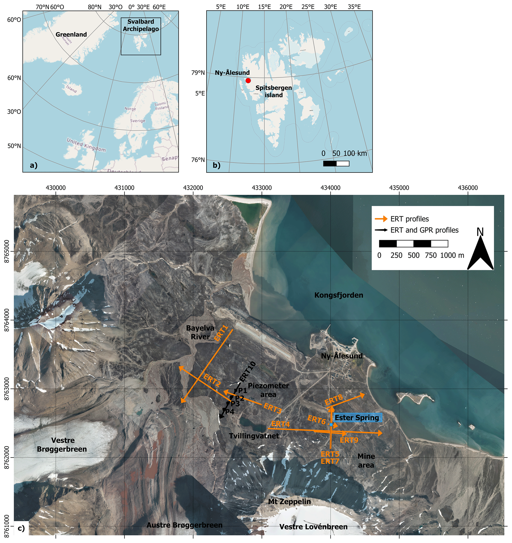
Figure 1(a) Location of the Svalbard Archipelago; (b) location of Ny-Ålesund on Spitsbergen, western Svalbard (© OpenStreetMap contributors 2023. Distributed under the Open Data Commons Open Database License (ODbL) v1.0); (c) general overview of the area investigated by the ICEtoFLUX project. The Ny-Ålesund settlement is close to the catchment of the Bayelva River. The orange lines represent the ERT profiles (from ERT1 to ERT10 and P1–P4). The black lines represent the profiles where both ERT and GPR were acquired. The coordinate system is WGS84-UTM33N. The satellite picture in the background was exported from the WebGIS tool by the © Norwegian Polar Institute (https://geokart.npolar.no/Html5Viewer/index.html?viewer=Svalbardkartet, last access: January 2024). Some of the acquisitions overlap fully or partially: two surveys were performed during July–August 2022 and August–September 2022 to possibly find some variations over time.
The history of this Arctic region is necessarily tied to the geoscientific exploration of pioneers driven by the thirst for knowledge or by the urge to run the (black) gold rush, as this land is rich in coal deposits (Dallmann, 2015). The geology of this area has been accurately investigated since the beginning of the 20th century, with a particular focus on the coal ore deposits that were exploited until 1962 (Hoel, 1925; Orvin, 1934).
The Svalbard Archipelago is located in the northwestern corner of the Eurasian Plate, as shown in Fig. 1a (Horota et al., 2023). The outcropping rocks in the Archipelago represent a natural geological archive of the Earth's evolution since its early history, from Archean to recent times. Major tectonic events affected the bedrock of the Svalbard islands including the Caledonian orogeny, which resulted in the deformation of the pre-Devonian metamorphic and sedimentary basement. Svalbard's sedimentary succession from Devonian to Paleogene is nearly complete and comprises a wide range of lithologies (conglomerates, sandstones, shales, carbonates, and evaporites). The main rock types are dated from Carboniferous and Permian (limestones and dolomites) to Tertiary sandstones (Fig. 2). Widespread moraine deposits occur in the study area.
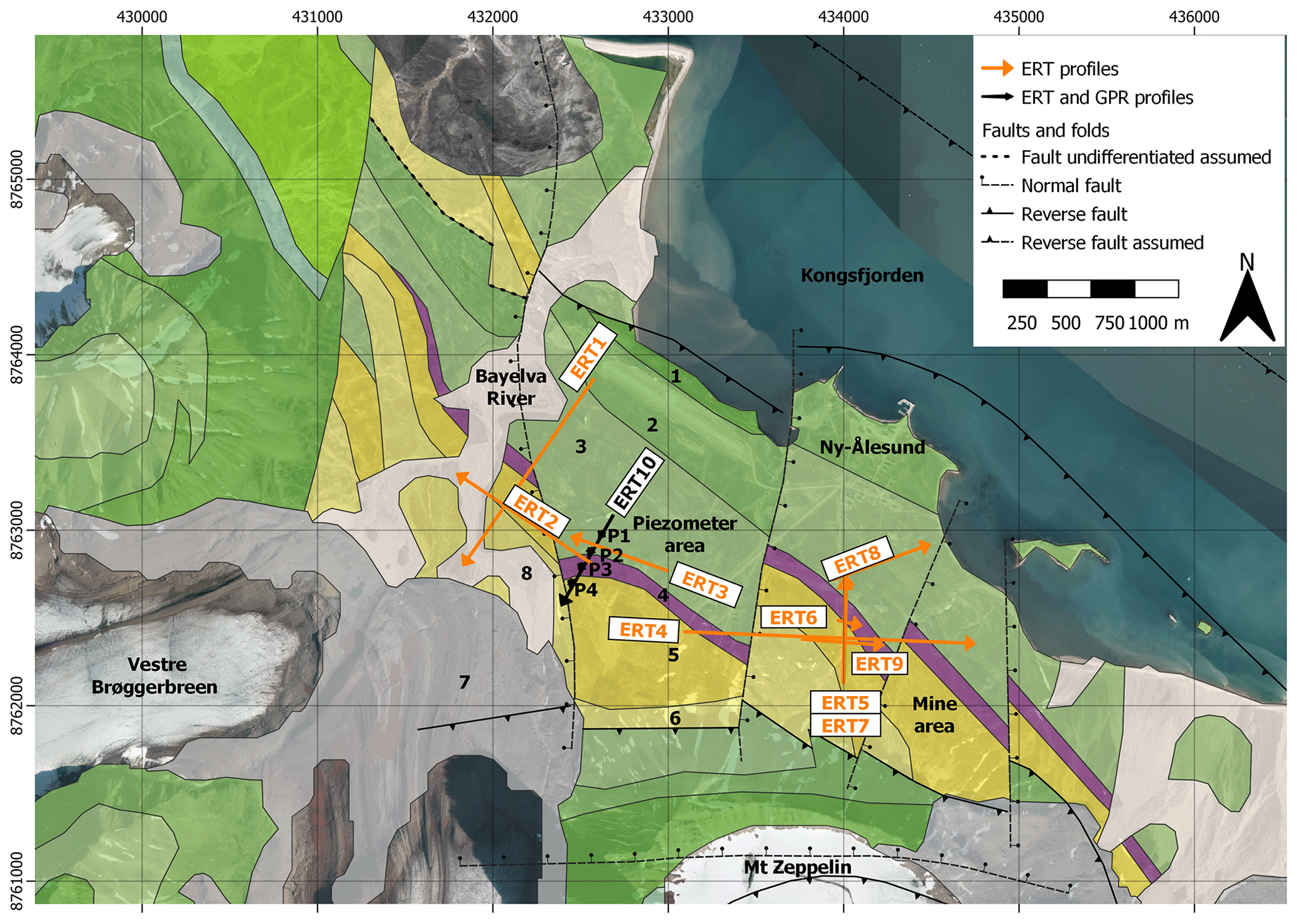
Figure 2Geological map (data from NPI, WMS geological map at 1:250 000): (1) carbonate rocks of Wordiekammen Formation (Moscovian–Sakmarian); (2) carbonate rocks of Gipshuken Formation (Sakmarian–Artinskian); (3) chert, shale, sandstone, and limestone of Kapp Starostin Formation (late Artinskian – late Permian); (4) shale, siltstone, sandstone of Vardebukta Formation (Induan); (5) sandstone, shale, coal of Kongsfjorden Formation (Paleocene?); (6) sandstone, shale, conglomerate of Brøggerbreen Formation (Paleocene?); (7) moraine (Holocene); (8) glacio-fluvial deposits (Holocene); (NF) normal fault; (RF) reverse fault. The coordinate system is WGS84-UTM33N. The geological map was exported from the WebGIS tool by the © Norwegian Polar Institute (https://geokart.npolar.no/Html5Viewer/index.html?viewer=Svalbardkartet, last access: January 2024).
In the 20th century, the area hosted the northernmost productive coal field in the world. The coal seams are of Tertiary age, Paleocene or Eocene (Hoel, 1925). Briefly, the strata consist of sandstones, with subordinate layers of conglomerates, shales, and coal. The coal seams are concentrated in the lower and upper parts of the Triassic sedimentary sequence (Orvin, 1934). In the lower coal horizon, the most important seams are (from bottom to top) the Ester, Sofie, and Advokat seams. The Agnes-Otelie, Josefine, and Ragnhild seams are on the upper horizon.
The mining exploration period (the first half of 20th century) left a heritage of information about the subsurface of Ny-Ålesund. Several pits and boreholes were drilled into the frozen soil to reach the coal seams. The depth of the pits was from 5 to 20 m, while for the boreholes it was up to 100 m. Relative information, stratigraphy, and geological sections, mainly reporting on shales, sandstones, and coal, are presented and accurately described in the appendix plates in Orvin (1934). The boreholes showed widespread permafrost conditions but were not intended to carefully assess the permafrost extension and spatial variability, which are hence not possible to be inferred.
Recent studies on the temporal variability of the permafrost have been performed by means of pits and borehole temperature monitoring. A comprehensive review of the permafrost monitoring activities near Ny-Ålesund can be found in the 2018 SESS report (Orr et al., 2019). An extensive 20-year borehole data set near the Bayelva River has been published by Boike et al. (2018) and highlights the recent climate variability in Ny-Ålesund.
Near the old mine area, southeast of Ny-Ålesund, between the fjord and the mountain of the Vestre Lovénbreen Glacier (Fig. 1c), recent changes in a complex sub-permafrost hydrological network have been studied (Haldorsen et al., 1996). During the mining period, Tvillingvatnet Lake, in the west side of the mining area, was reported to receive influx water from a sub-permafrost aquifer. During winter, the lake was not frozen, and the miners discovered a confined aquifer nearby. The sub-permafrost aquifer was fed by glacier waters, probably by the nearby Austre Brøggerbreen, which extended closer to the lake than today (see Fig. 1c). Today, Tvillingvatnet Lake freezes during winter, thus suggesting that the sub-permafrost influx has apparently stopped or is greatly reduced. Chemical analyses of the lake water showed that it now probably comes from a supra-permafrost aquifer located on the hillside of the Vestre Lovénbreen mountain (Haldorsen et al., 2002). A similar fate befell Ester Spring, located in the mine area (see Fig. 1c). This spring was reported from the mining period (around 1930) and was characterized by a continuous water flux of multiple liters per second during winter and constant chemical properties during the year. The spring water was assumed to come from the Vestre Lovénbreen Glacier, to infiltrate into a moulin, and then to be heated underground by the geothermal heat. This made it possible to warm the permafrost and to generate Ester Spring (Booij et al., 1998; Van der Ploeg, 2002). This flux decreased over the past few decades and then stopped in 2007. According to the literature, the recent changes observed in Ester Spring are linked to the global warming effects on the Vestre Lovénbreen Glacier (Haldorsen et al., 2011, 2010; Haldorsen and Heim, 1999). Due to the warming temperatures and thinning of the glacier, it has lost part of its insulation effect against the cold winter (Pälli et al., 2003). Therefore, the geothermal heat flux is no longer able to keep the glacier base at the pressure–temperature melting point, and the water and heat transfer from the moulin to Ester Spring may have stopped (Putkonen, 1998). Supporting this hypothesis, a water flux larger than the past is observed melting at the tongue of the glacier through superficial streams, while in the past the melting at the tongue was minimal.
All of the aforementioned studies, while having delved into specific aspects of the permafrost processes, rely on a few deep boreholes or focus on specific areas in the surroundings of Ny-Ålesund. Therefore, currently it is not possible to provide a comprehensive overview of the spatial variability of the permafrost in the study area, especially at significant depth. In this context, the proposed shallow and deep geophysical investigations (ERT and GPR), which ensure different resolution scales, can fill the knowledge gap regarding the spatial variability of the permafrost, potentially uncovering features that have not been discovered to date.
The geophysical survey of the I2F project was conceived in parallel with hydrogeological investigations. The four piezometers (P1, P2, P3, P4) drilled as part of the I2F project (see the “Piezometer Area” in Fig. 1c) were placed in a dominantly mineral soil in order to monitor continuously the water level, temperature, and electrical conductivity of the water, to measure periodically the depth of frozen ground, and to sample water for chemical and isotopic analyses. High-density polyethylene pipes (with a diameter of 63 cm and a length of 3 m) were inserted in predrilled holes down to 200 cm into the soil. Each tube was screened by 3 mm slits in the lower 200 cm to allow water to enter the tube. Once piezometers were installed, caps were placed on top, again preventing outside material from entering the tube. The gravel (2–5 cm in diameter), collected locally to avoid external effects on the chemical features of the water, was placed between the tube and the soil to fill the space around the tube and create a pre-filter with respect to the screened part. The piezometer metadata are available from the Italian Arctic Data Center (IADC) website (https://metadata.iadc.cnr.it/geonetwork/srv/api/records/5e0ba64e-71a7-4949-8752-9fb57b38b4fa. last access: May 2024). Moreover, the I2F website shows the location and coordinates of the piezometers, the network of sampling stations (snow pits, glacial and proglacial drainages, bulk snow), and geophysical surveys (https://www.icetoflux.eu/data/, last access: May 2024). This page will provide the piezometer data from continuous monitoring (including chemical and isotopic water analyses) as soon as the hydrological modeling is completed by the project partners. Some of the piezometer data measured during the geophysical surveys, such as depth of frozen ground, water level, and water electrical conductivity and temperature, were used for preliminary interpretation of the geophysical results of this work. Meteorological and climatic data (air temperature and precipitation) can be downloaded from the Ny-Ålesund weather station (SN99910, https://seklima.met.no, last access: May 2024).
3.1 ERT and GPR methods
ERT is an active geophysical technique that involves the injection of current into the subsoil and the measurement of the consequent voltage distribution at the surface. The current is injected in a dipole of electrodes, called “transmitter” or “source”, while the voltage is measured at one or multiple dipoles, called “receiver” (or “receivers”). The measured voltage is influenced by the current flowing in the subsoil, which is, in turn, dependent on rock types, porosity, water saturation, salinity and temperature, weathering, metallic content, and clay content. The transmitter and the receivers can be placed in several relative positions or configurations. Different configurations are sensitive to different patterns of resistivity distribution. In the Ny-Ålesund survey, three configurations were employed: Wenner (WE), Wenner–Schlumberger (WS) and dipole–dipole (DD). While WE and WS are sensitive to the vertical layering of the subsoil, DD is sensitive to lateral resistivity contrasts (Martorana et al., 2017). The distance between the electrodes affects the depth of investigation of a measurement, the vertical penetration of the injected current, the lateral resolution of the data, and the field logistics. The greater the electrode spacing, the greater the depth of investigation and the lower the data resolution in the near surface (Oldenburg and Li, 1999). We chose electrode spacings of 1 and 2 m to characterize the region of the active layer and of 10 m to characterize the expected permafrost layers or deep aquifers at the expense of high resolution in the near surface.
GPR is a non-invasive methodology that detects electromagnetic (EM) impedance differences in a medium. It is based on the analysis of the reflections of electromagnetic waves transmitted into the ground depending on the frequency of the electromagnetic waves and the electrical characteristics of the potential targets and surrounding soil (electrical permittivity and conductivity). The use of different antennas and frequencies enables the imaging of subsoil at different penetration depths: the lower the frequency, the larger the penetration depth. Therefore, the operating frequency is always a trade-off between resolution and penetration depth. In our survey, the GPR acquisition was planned to retrieve high-resolution information at a relatively shallow depth. Two antennas with different frequencies were adopted: 400 and 40 MHz. The emitted signal at high frequency (400 MHz) allows for detailed information up to 4 m depth, which is enough to image the expected interface between the active layer and the permafrost. The 40 MHz signal was planned to reach 10–20 m depth (Jol, 2009).
3.2 MT method
The MT method is a natural-source electromagnetic method that measures the Earth's response to the low-frequency EM waves coming from the magnetosphere and ionosphere. Measurement of the electrical and magnetic fields makes it possible to determine the electrical resistivity of the Earth at depths ranging from some meters to hundreds of kilometers (Chave et al., 2012). The acquisition of MT data is performed with no transmitters since the signal has a natural origin. Two horizontal components of the electric and magnetic fields are measured on the ground surface. The electric field is measured by means of two pairs of dipoles (grounded non-polarizable electrodes), with the direction of one pair usually being parallel to the magnetic north (x direction for MT convention). The magnetic field components are usually measured by means of two horizontally buried magnetometers (induction coils). A third additional magnetometer can be deployed to measure the vertical component of the magnetic field.
The audio-MT method (AMT) refers to the measurement of MT signals in the frequency range from 105 to 10 Hz. AMT is devoted to the shallow characterization of geoelectrical structures. The broadband MT method refers to measurements of both low and high frequencies usually in the range of 103–10−4 Hz with deeper investigation depths than AMT.
For our geophysical survey, two different systems were adopted for AMT and broadband MT acquisitions. The AMT equipment was composed of the Geometrics StrataGem system, two G100K magnetometers, and four steel electrodes. The broadband MT equipment was tailored by Zonge International Inc. and consisted of one ZEN receiver (high-resolution, multichannel 32-bit receiver) that records broadband time series from 103 to 10−4 Hz, three magnetometers (type ANT/4), and six non-polarizable electrodes (Pb-PbCl) devoted to geophysical resistivity measurements.
The MT and AMT surveys were planned to be carried out during the I2F project because they have different resolution and depth of investigation with respect to ERT and GPR. MT and AMT were deemed to be ideal for the deep characterization of permafrost and sub-permafrost aquifers since they are more sensitive than ERT and GPR to electrically conductive formations and have a larger depth of investigation than ERT and GPR. Moreover, the MT and AMT methods were assumed to overcome the possible difficulties of the ERT method related to the injection of a direct current into a highly resistive subsoil like the one expected in Ny-Ålesund. There are several MT and AMT applications that study the ice sheet and glacial dynamics in the polar regions (Hill, 2020), in both Arctic (Beka et al., 2015, 2016, 2017a, b) and Antarctic regions (Wannamaker et al., 1996, 2017).
The MT and AMT surveys were planned in the Bayelva and mine areas, but every attempt of acquisition had no success. The planned MT and AMT surveys had to be stopped after the acquisition of five soundings due to an unexpected high level of anthropic electromagnetic noise. The first MT acquisition was scheduled with three different sampling rates for a total of 2.5 h. The estimated impedances ranged in the frequency band from 0.01 to 1280 Hz but were affected by noise. Then, four AMT soundings were acquired, but – again – the data were corrupted by noise. The AMT time series were processed by using different window lengths and filtering stages in three frequency bands, resulting in impedance estimates in the frequency range from 15.8 Hz to 63 kHz.
The MT data would have been useful for the deep characterization of the permafrost and potential sub-permafrost aquifer. However, the MT and AMT data processing performed after the first acquisition revealed a wide-band and energetic noise source whose presence prevented the possibility of acquiring good-quality MT data. This was completely unexpected because Ny-Ålesund is a radio-silent and geographically remote settlement, where wireless equipment is not allowed so as to ensure a high signal-to-noise ratio for the data measured. Even though any equipment emitting radio signals is avoided and several scientific instruments take advantage of the radio silence, a few exceptions are permitted for safety, operational, and scientific reasons. The equipment transmitting and receiving radio frequencies in Ny-Ålesund is supposed to be authorized and listed in the “NySMAC frequency list” (https://nyalesundresearch.no, last access: April 2024). Although the listed equipment operates in the frequency range from kilohertz to gigahertz, it directly or indirectly affected the quality of our acquired MT signals in the frequency bands > 1 Hz. As an example, this low quality can be appreciated in Fig. 3, where the power spectra are dominated by a 50 Hz noise and its harmonics. The signal in Fig. 3 was analyzed in MATLAB® Signal Processing Toolbox. The presence of this kind of noise made it impossible to obtain reliable MT estimates. Note that in Fig. 3 the time series of the magnetic components are not deconvolved for the instrumental response.
Therefore, the MT and AMT surveys were shut down and the data were not included in the repository published with this work since it was not possible to process and interpret them. However, our experiment can be of help for future geophysical expeditions in Ny-Ålesund.

Figure 3Time series (a) and power spectra (b) related to the electric (Ex and Ey) and magnetic (Hx and Hy) field components sampled at 4096 Hz. Ex is plotted in ochre, Ey in purple, Hx in green, and Hy in cyan. The components were measured in the (magnetic) N–S and E–W directions. The signal was analyzed in MATLAB® Signal Processing Toolbox.
3.3 Data acquisition
Three different sectors around Ny-Ålesund were surveyed (Fig. 2): (i) the Bayelva catchment on the west, (ii) the piezometer area close to the Amundsen–Nobile climate change tower (CCT), and (iii) the mine area on the east (close to Ester Spring).
The geophysical survey had to be planned to overcome specific logistic difficulties owing to the study area being located in a remote polar region and to the long duration of the survey, which was divided into two different campaigns during the thaw season. First, all of the equipment (14 boxes with a total weight of around 450 kg) had to be shipped 2 months before the survey and returned 3 months after the survey ended. Second, the whole crew had to obey the health and safety protocol, which is required in order to be hosted in the Italian Arctic Station and to carry out field operations in a region where polar bears may approach humans. Globally, field logistics and fieldwork conditions were largely affected by the isolation and asperity of the study area. For example, most of the survey sectors were not directly accessible from the road, and hiking with the equipment was necessary. Moreover, since safety was of primary concern, operators had to work nearby to monitor the presence of wildlife (polar bears) in the surroundings, thus extending the time required for the surveys.
The ERT survey was divided into two campaigns between July and September 2022. The instrument was the georesistivimeter Syscal Pro (Iris instruments). The receiver was multichannel with a maximum of 10 measurements at a time and a maximum number of 48 electrodes for each acquisition. Standard stainless steel electrodes were used. The configurations of the acquisition were DD (both in direct and reverse configurations), WS, and WE. The acquisition was usually moved forward by using the roll-along technique. The acquisition settings of the instruments were an injection time of 500 ms and a minimum number of 3 up to 6 stacks. The accepted error percentage on the stacks was 2 %. A total length of 7.87 km was acquired along 18 profiles (Fig. 1c and Table 1). The electrode spacing was 10 m for 9 profiles (deep ERTs), 1 m for 8 profiles, and 2 m for the remaining 1 profile (shallow ERTs). Details on the acquired ERT profiles are listed in Table 1.
The soil conditions were generally fair in terms of electrical contact resistance, allowing us to easily achieve contact resistance values lower than 10 kΩ. This was not surprising because the thaw season is generally the best season for ERT data quality, since the contact resistances are expected to be low (Herring et al., 2023). Not favorable conditions were encountered in areas where stones and gravel covered the ground surface, such as in the Bayelva catchment and in the mine area. The bentonite was used there to improve the ground–electrode contact, if necessary. For some of the profiles the contact resistance values were stored together with the data to enhance a posteriori control of the data quality (see Sect. 4.1). The contact resistance was stored only for the WS acquisitions due to the negative influence that this procedure has on the multichannel acquisition (i.e., the DD acquisition) in terms of time consumption.
Table 1Data acquisition parameters and array configuration for ERT profiles. The coordinate system is WGS84-UTM33N.
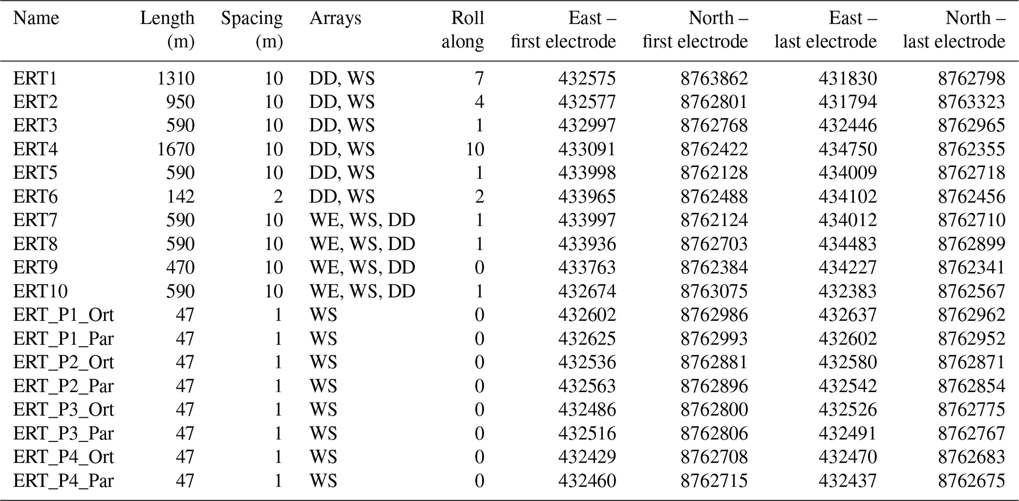
The two 10 m spacing profiles in the Bayelva catchment (ERT1 and ERT2) are perpendicular and very close to the Bayelva River, which is crossed at the end of the two ERTs toward the glaciers. In the area of the piezometers, there are two perpendicular 10 m spacing profiles (ERT3 and ERT10) and eight short profiles (1 m spacing) that cross the four piezometers (P1, P2, P3, P4) in parallel and orthogonally. Then, the mine area is crossed by the longest line, ERT4 (1.67 km), which partially overlaps with ERT9. Three profiles cross Ester Spring (ERT5, ERT6, ERT7) and a profile is directed towards the sea (ERT8). ERT7 and ERT5 are partially coincident because they were measured during two different campaigns, in July and September 2022, respectively. The same applies to ERT9 and ERT4, respectively. ERT6 was acquired with 2 m spacing.
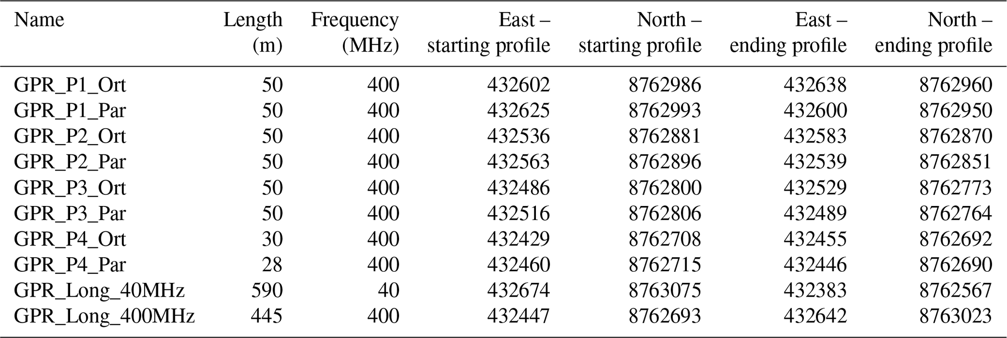
The GPR data were acquired with the GSSI SIR-3000 GPR System coupled with two different antennas working at the frequencies of 40 MHz (SUBECHO AB Sweden air-coupled antenna) and 400 MHz (GSSI ground-coupled antenna). The adopted recording time window is set to 120 ns for the acquisition performed with the 400 MHz antenna and 1200 ns for the data acquired with the 40 MHz antenna. The acquired data were discretized by 512 time samples. Since the acquisitions were carried out without a survey wheel, the data were acquired in time domain and several marks were placed every 5 m in order to assign the right coordinates to each recorded trace. The GPR survey was carried out in the piezometer area, as shown in Fig. 2. The cumulative surveyed length is about 1400 m along 10 GPR lines. Each line has been measured in a direct and reverse sense for a total surveyed length of 2800 m. The 400 MHz antenna was used to measure GPR radargrams along the eight shallow ERT profiles centered in the four piezometers (P1, P2, P3, P4) and along the ERT10 line crossing all the piezometers. The antenna at 40 MHz was adopted for a line corresponding to ERT10. Details on the acquired GPR profiles are listed in Table 2.
The surface investigated close to the piezometer area was regular and the few ground irregularities encountered did not affect the quality of the acquired data, always ensuring a proper surface contact for the ground-coupled antenna. The use of the 400 MHz antenna was limited to the transect line where it was possible to guarantee adequate contact between the ground and the antenna, avoiding unwanted “jumps” of the antenna itself. This limitation did not affect the use of the 40 MHz antenna, which performs well even in the absence of direct contact with the ground.
4.1 Raw data and quality control
As a standard practice, each acquisition of ERT data was preceded by a check of the contact resistance between the electrodes and the ground. This operation (“RS check”) was directly performed by the instrument. As an additional quality control (QC), specific electrodes (occupying a known position along the geoelectrical lines) were unplugged before starting the contact resistance check in order to verify the correct number and addresses of the electrodes. When one of the unplugged electrodes was involved in the RS check, the georesistivimeter stopped the check operation as long as the electrodes were correctly plugged. The contact resistance values of ERT7, ERT8, ERT9, and ERT10 and of ERT_P1, ERT_P2, ERT_P3, and ERT_P4 were stored together with the WS geoelectrical data to enhance a posteriori QC and monitoring of the measuring conditions.
At the end of each ERT survey, an in-field evaluation of the collected data quality was performed. The data were downloaded from the georesistivimeter and visualized as pseudosections of apparent resistivity (see Fig. 4a for example). The regularity of the data distribution in relation to the measuring conditions was used to drive decision-making on the necessity of repeating the data acquisition or changing the investigation strategy.
Noisy data in the geoelectrical measurements can be due to soil conditions, complex subsoil structures, or instrumental failure. Soil conditions can negatively affect the ERT data if the ground–electrode electrical contact is not ideal. This condition is common in those areas where stones and gravel cover the ground surface, such as in the Bayelva catchment and in the mine area. Bentonite was used to improve the ground–electrode contact when needed.
The QC on the field for the GPR data was aimed at verifying the proper functioning of the GPR acquisition system (control unit and antennas) and the correct settings of the acquisition parameters (time window, sampling rate, gain, trace increment, etc.). The QC was preliminarily done, during the data acquisition process, directly on the GPR acquisition system monitor. Subsequently, a more thorough verification was performed in the laboratory after the acquisition, resulting in the elaboration of preliminary 2D radargrams.
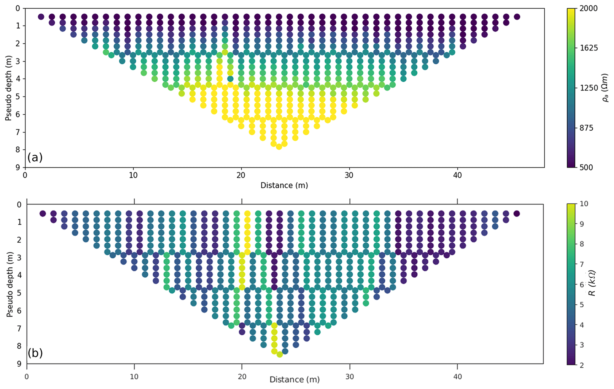
Figure 4Example of experimental pseudosection of the ERT_P1_Par profile. The acquisition configuration is WS: (a) spatial distribution of the measured apparent resistivity (ρa) values (in Ωm); (b) contact resistance values (in kΩ) recorded for each pair of current electrodes involved in the data acquisition sequence.
4.2 Processed data
The ERT data were pre-processed by using the software Prosys-III (Iris Instruments). The filtering procedure for the ERT data was based on the verification of some general criteria. For each geoelectrical profile the preprocessing consisted of discarding the following data:
-
electrodes with anomalous values of contact resistance (“RS check”), when available;
-
negative resistivity values;
-
isolated extremely high or low resistivity values (i.e., outliers).
An example of ERT data with the pseudosections of apparent resistivity and contact resistance with a WS configuration is depicted in Fig. 4 for profile ERT_P1_Par. It is centered at piezometer P1 and is parallel to ERT10. This profile was chosen as representative since GPR data were acquired at the same location (see Sect. 5.2). The apparent resistivity pseudosection (Fig. 4a) is characterized by relatively smooth variations and no outlier data as expected considering the good contact resistances (Fig. 4b). The filtered ERT data were then ready to be inverted to create 2D geoelectrical models of the subsoil (see Sect. 5.1). The whole set of pseudosections measured along each ERT is presented in the repository (see Sect. 6 for details).
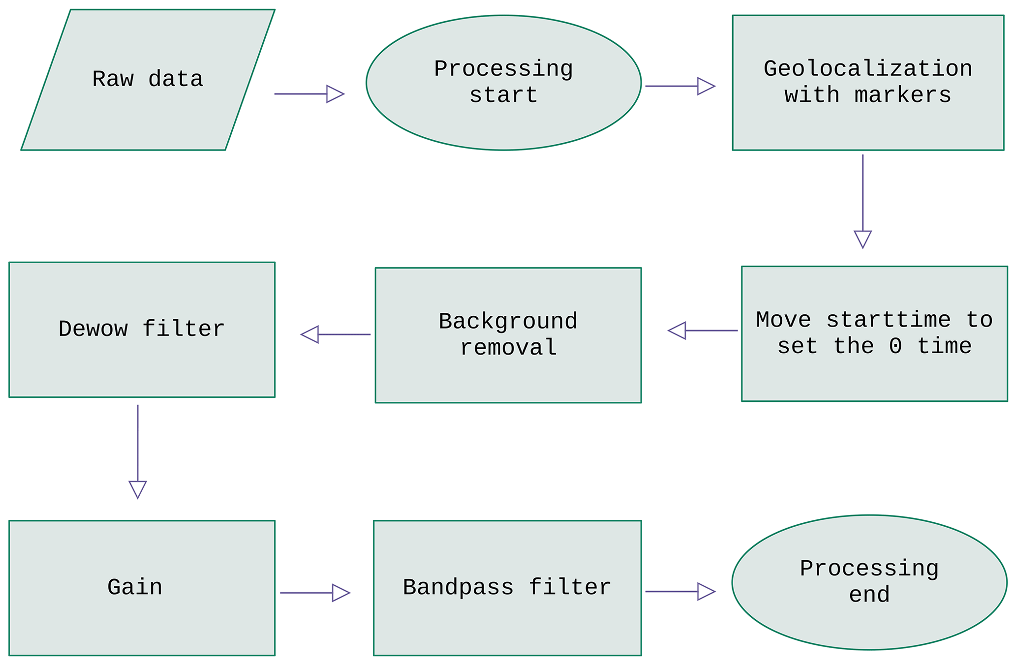
The GPR data were processed with Reflexw software (Sandmeier, 2021), according to the processing chain depicted in Fig. 5 and accurately explained as follows:
-
The distance between each trace was set in order to match, every 5 m, the geolocation of the marker, with the “marker interpol.” processing step.
-
A time-zero correction was performed, with the “move startime” processing step, by manually selecting, as time zero, the value in nanoseconds corresponding to the beginning of the transmitted impulse.
-
A background removal filter was applied over the whole profile, subtracting the average trace from each trace.
-
A subtract-mean, or “dewow” filter, was used with a time window of 2 and 8 ns for 400 and 40 MHz data, respectively, to remove possible instrumental voltage shift in the data.
-
A manually selected gain function, based on the operator's choice and experience, was applied to contrast the effects of signal attenuation and geometric dispersion.
-
A bandpass filter removed the frequencies below about 150 MHz and above about 550 MHz for 400 MHZ data and between 20 and 100 MHz for 40 MHz data.
-
Only for the 40 MHz data, an automatic gain control (AGC) with a time window of 100 ns was applied in order to better detect deep reflectors.
For visualization, the topography of all GPR data was corrected by using the topographic surface retrieved from a recent digital elevation model with 5 m resolution, published by the Norwegian Polar Data Centre and available as basemap data “Svalbard digital elevation models” at https://geodata.npolar.no (last access: January 2024, © Norwegian Polar Institute, 2014). Each radargram was normalized to its amplitude mean value.
5.1 ERT inversion method
The ERT data pre-processing and filtering of the outliers is usually followed by the geophysical inversion of the acquired data. The inversion aims at finding the best resistivity distribution of an Earth model which explains the data within a certain error threshold.
The 2D ERT inversion was performed by using the open-source package ResIPy (Blanchy et al., 2020). ResIPy can be used for geoelectrical data (direct-current and induced polarization measurements) and provides several tools such as high-level filtering, error modeling, 2D and 3D inversion/forward modeling, and post-processing. It can be accessed from a Python application programming interface (API) or a stand-alone graphical user interface (GUI). Further information about ResIPy and other software for electrical resistivity modeling can be found in Doyoro et al. (2022) and Loke et al. (2013).
In the inversion process, the same mesh discretization was adopted in terms of cell growing factor, characteristic length, and background resistivity. The boundary depth of the model was 80 m for the ERT lines with 10 m spacing between the electrodes. The cell growth factor was 7. The characteristic length was kept as the ResIPy default to ensure two mesh nodes between two consecutive electrodes. The topography was included. The inversion type was a regularized inversion with linear filtering and normal regularization. The same inversion settings were adopted for all the quadrupole configurations (WE, WS, DD). The only exception was for the measurement errors given to the inversion. For the WE and WS data sets, the data error was set to 2 %, in agreement with the largest observed stacking errors. For the DD data sets, an ad hoc error model (linear or power law) was calculated from reciprocal error distribution and then used in the inversion procedure.
The number of iterations was between 2 (for short profiles) and 10 (e.g., for the longest ERT4), all computed in a few seconds. The final root mean square errors (RMSEs) ranged between 1 (the minimum threshold to end the inversion) and 2.18 (for ERT4, which had high errors).
5.2 ERT models
The inversion result for the ERT_P1_Par (WS configuration, 1 m electrode spacing) is presented in Fig. 6. The resistivity model shows a gradual increase in resistivity with depth. At shallow depth, up to 2 m below ground level (b.g.l.), the resistivity range is 100–500 Ωm, while from 2 m depth down to the bottom of the model the resistivity rises to 1000 Ωm and even up to 8000 Ωm, which can be theoretically correlated with the permafrost. The resistivity model of Fig. 6 does not show a marked lateral variability, that is, the resistivity clearly increases with depth, being characterized by a shallow medium resistive layer and a deep very high resistive layer. This geoelectrical structure is valid only for profile ERT_P1_Par because the measured apparent resistivity data in the ERT profiles centered in the other piezometers are clearly different. Further interpretation of the resistivity models goes beyond the scope of this paper and needs multidisciplinary contributions, given that the resistivity of the frozen rock might be site specific. To the best of the authors' knowledge, there is no direct measurement of electric resistivity in the investigated area, except for a few old and superficial electric conductivity sensors installed at up to 1 m depth in the Bayelva Basin (Kodama et al., 1995; Boike et al., 2018; Son and Lee, 2022).

Figure 6Resistivity model obtained from the inversion of ERT_P1_Par. The acquisition configuration is WS. The minimum and maximum boundaries of the color bar are 100 and 3000 Ωm, respectively.
Another representative example of results is ERT9, which was acquired with 10 m electrode spacing and with different quadrupole configurations (DD, WS, WE). ERT9 is located in the mine area and close to Ester Spring. The inversion results for ERT9 are presented in Fig. 7. The general picture presented by the three models is basically the same, but the DD (Fig. 7a), having a higher lateral sensitivity and data coverage, offers a more resolved picture of the underlying electrical structure. Among the three models, the less informative one seems to be WE (Fig. 7c), which greatly resembles the WS model (Fig. 7b) but with low resolution in terms of spatial data coverage and array characteristics. The reliability of the inversion results is derived not only from the similarity of the three geoelectrical models of Fig. 7, but also from the pseudosections of the contact resistance (stored with the WS data), as shown in Fig. 8a, and of the percentage reciprocal error (derived by measurements in DD direct and reverse configuration), as shown Fig. 8b.
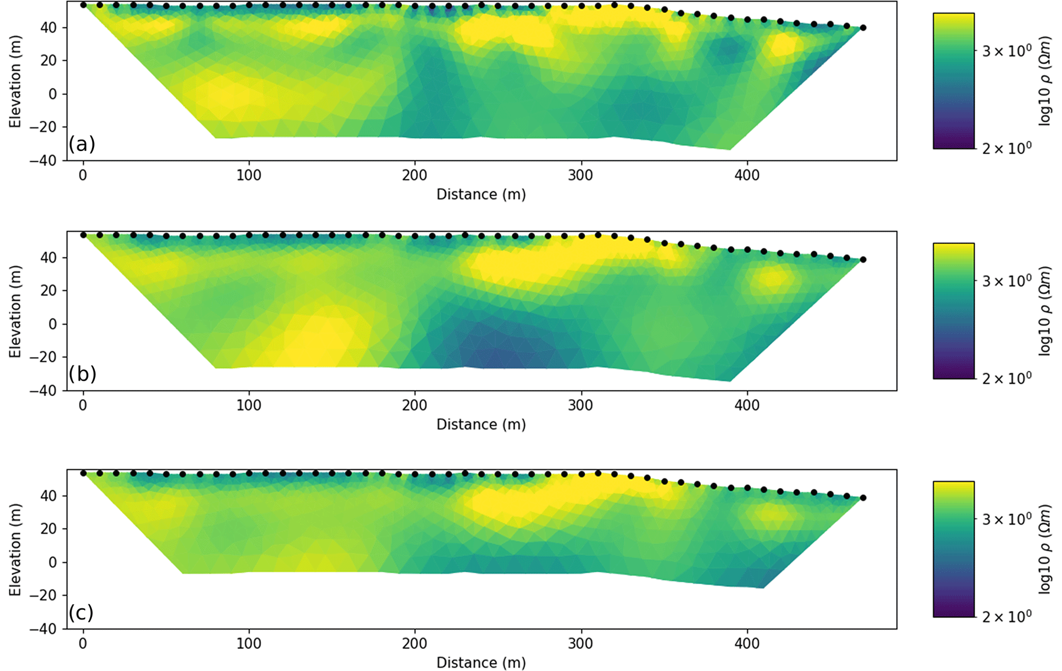
Figure 7Resistivity model obtained from the inversion of ERT9. Different acquisition configurations: (a) DD, (b) WS, and (c) WE. The minimum and maximum boundaries of the color bar are 100 and 3000 Ωm, respectively.
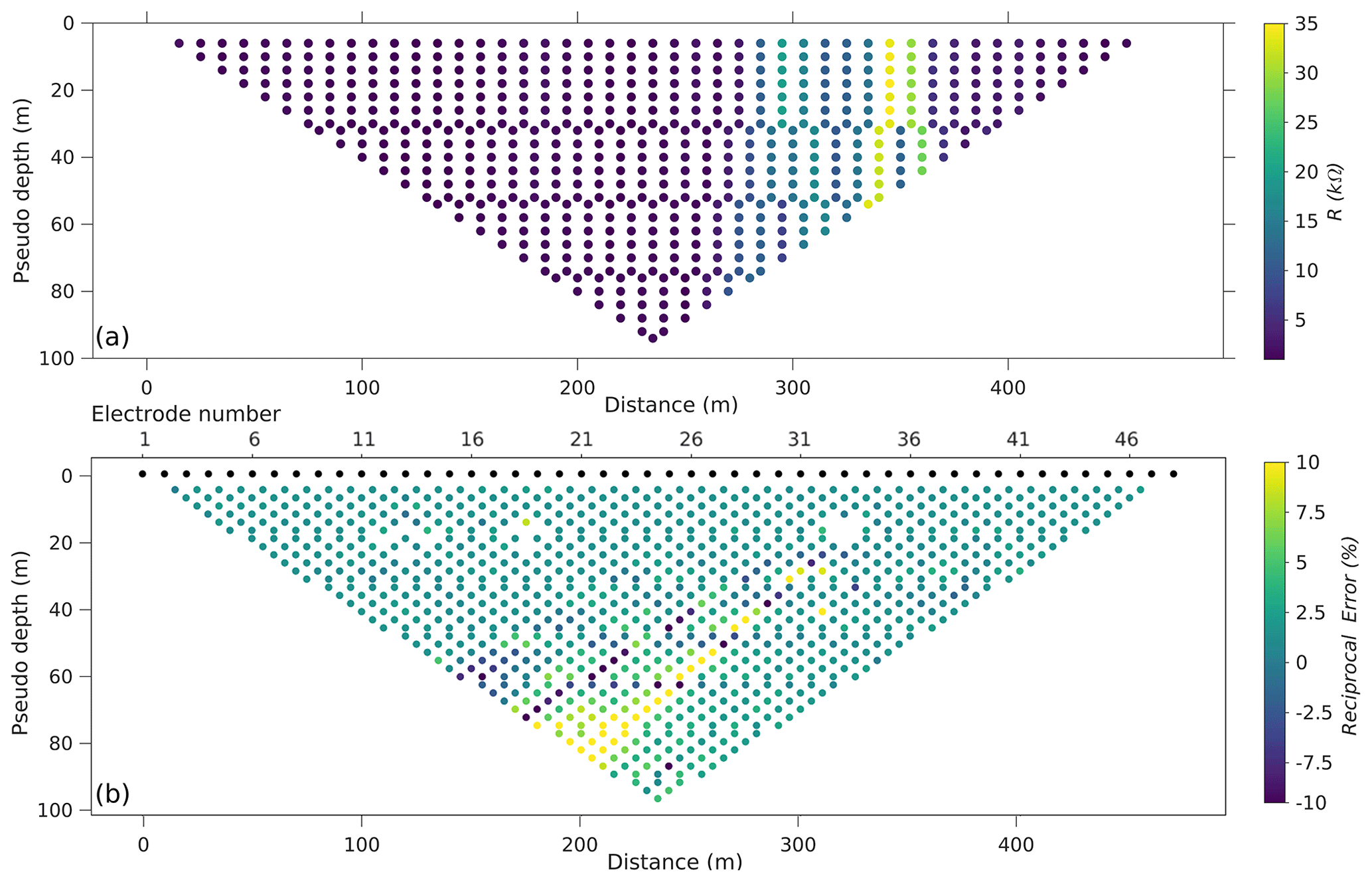
Figure 8Pseudosections of ERT9 for (a) contact resistances stored during the WS acquisition and for (b) percentage reciprocal errors derived from the DD acquisitions performed in direct and reverse configurations.
As regards the quality of the ERT data, different levels of noise and error were recognized. For example, Fig. 8b represents for ERT9 the pseudosection of the percentage reciprocal errors that are in the range of ±2.5 % for most of the data points and reach ±10 % for some of them at 60–90 m pseudo-depth. The pseudosections from the Bayelva catchment presented reciprocal errors up to ±40 % (see the figures “ReciprocalError.png” in folders 2_Filtered_ data_inversion_input/DD in the repository). By contrast, the pseudosections of the percentage reciprocal errors in the piezometer area showed the lowest values, with a maximum of ±4 % (for example, see ERT10, DD acquisition in the repository). Given that the quality of ERT data was heterogeneous among the different profiles, the data set provided in the repository includes the raw data as well as processed/filtered ERT data ready to use. The raw data can be inspected for each line to allow the user to assess the original measurement errors (stacking errors) or the reciprocal errors and then potentially reprocess them according to different criteria.
The post-processing analysis of the inversion results was carried out in MATLAB®, where we imported the ResIPy output (that is, the file “f001_err.dat”) to plot the spatial distribution of apparent resistivity (observed and calculated) and the errors. The MATLAB script to generate this kind of figure is provided in the repository for reproducibility, in the folder “ERT/Example results”, under the name “Post_processing_Matlab.pdf”.
Figure 9 shows an example of post-processing for ERT_P1_Par (WS configuration). There is no topography in this kind of representation, since the vertical axis is a pseudo-depth. The three panels illustrate (a) the pseudosections of measured data, (b) the computed apparent resistivities, and (c) the misfit between them. The pseudo-depth was calculated following Edwards (1977), that is, the same approach adopted in ResIPy (Fig. 4). The computed response is the apparent resistivity values that one would obtain performing a measuring operation on a subsoil in which the resistivity is distributed exactly as in the calculated resistivity model in Fig. 6. The lower the misfit between the observed and calculated data, the higher the reliability of the inversion result.
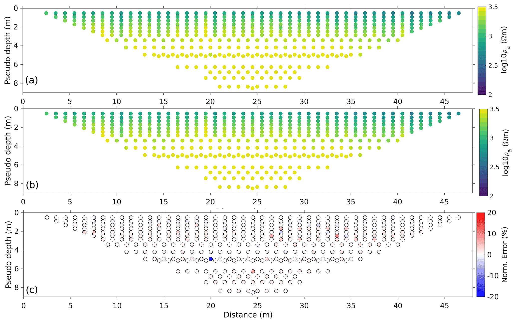
Figure 9Post-processing analysis of the ResIPy inversion result for ERT_P1_Par, WS configuration: (a) observed data (ρa); (b) calculated response (ρa); and (c) misfit between them, calculated as normalized error in percentage.
5.3 GPR results
Figure 10 shows GPR_P1_Par, a representative GPR line that is parallel to ERT_P1_Par and acquired with the 400 MHz antenna. The radargram is acquired close to piezometer P1 and unequivocally shows the presence of a reflective layer placed in a time window ranging between 50 and 55 ns. In order to convert the data from the time domain to the spatial domain, it is necessary to determine the propagation speed of the radar waves in the investigated levels. This is mainly related to the physical–electrical characteristics of the investigated medium. In particular, in a low-loss material, it is inversely proportional to the square root of the dielectric constant (εr) and is estimated or calculated through various possibilities of signal analysis or with experimental calibration tests. From the analysis and fitting of the hyperbolae characterizing the radargrams (Rønning, 2023), generated by punctual elements present in the subsoil (i.e., stones), it was possible to determine that the velocity value can be assumed equal to 0.10 m ns−1. This assumption was also validated by the comparison of the most reflective layer detected by the GPR data with the most interesting electrical anomalies detected by ERT at a similar depth. Further efforts are required to constrain the interpretation with the direct data that will be collected in the close piezometer P1.

Figure 10Example of a processed 2D radargram for GPR_P1_Par, which is parallel to ERT_P1_Par and was acquired with the 400 MHz antenna. The radargram is shown in two different color scales.
Figure 11 shows the results obtained with the 40 MHz antenna for profile GPR_long_40, which is the only one acquired at low frequency. The radargram was acquired with an antenna that does not require ground contact. Although the recorded signal is noisier than that acquired with the 400 MHz antenna and the resolution is not comparable to that provided by the 400 MHz antenna, some reflective layers can be detected in the upper 300 ns. After this time, the presence of attenuation phenomena does not seem to provide the possibility of identifying hydrogeological features. However, some discontinuities seem to characterize the radargram in particular at 450 m distance from the starting point of the radargram, where there is Bayelva River. Although Figs. 10 and 11 do not include the depth scale, all the processing details are provided in Sect. 4.2 for both antennas (40 and 400 MHz). The values for the processing reported in Sect. 4.2 can be applied to the GPR data acquired at 400 MHz, as the presence of some hyperbolae enables the estimation of the EM wave velocity. The GPR data acquired at 40 MHz reach a depth of investigation significantly greater than that at 400 MHz. The absence of clear reflectors (hyperbolae) and the scarce availability of prior hydrogeological information prevented the assumption of a single value for the migration of the radargram, which would have yielded an excessive simplification potentially inconsistent with the expected heterogeneity of the subsurface.

Figure 11Example of a processed 2D radargram for GPR_long_40 MHz radargram. The radargram is shown in two different color scales.
This section is mainly intended for readers interested in downloading and reusing the data. The aim is to provide raw and processed data in formats that are friendly for geophysical software, in order to allow geoscientists to visualize them best and reprocess them. We also provide the two representative inversion models shown in Figs. 6 and 7 as ready-to-use profiles of electrical resistivity of the subsoil, for scientists interested in direct use of the results for multidisciplinary studies, e.g., to produce geologic or hydrogeologic models, and for comparison of different inversion schemes. The coupled data sets of ERT and GPR data along the nine coincident profiles can also be used to test different joint inversion schemes.
6.1 Repository organization
The repository is organized in two main folders, as shown in Fig. 12: ERT and GPR (the folder names are highlighted in bold italic). The subfolder Data in ERT contains 18 subfolders, one for each deep ERT (from ERT1 to ERT10) and for each shallow ERT close to the four piezometers (from ERT_P1_Par/Ort to ERT_P4_Par/Ort). With regard to the latter, the notations “Ort” and “Par” refer to orthogonal and parallel directions with respect to the ERT10 that crosses the piezometers, respectively. Schematic information on the ERT profiles is given in Table 1. The scheme of the folder organization is depicted in Fig. 12.
Each of the 18 ERT folders contains the following subfolders:
-
1_Raw_data: this contains .bin files, as saved by the Syscal Pro georesistivimeter. The .bin files contain the elevation information for each electrode and its relative position in the line. The files do not include the geographical east and north coordinates of the electrodes.
-
2_Filtered_data_inversion_input: this contains a .Dat file which is the classic input format for performing the inversion in RES2DINV software (Loke, 2004; Loke and Barker, 1996), also readable by ResiPy. This folder contains the ResIPy project file (.resipy) with the embedded electrode coordinates, the topography, the mesh created for the inversion, and the inversion settings and results. The folder stores a .png image of the pseudosection of the apparent resistivity. For DD surveys, the evaluation of the reciprocal error was calculated, that is, the difference between resistivity measurements performed on the same quadrupole but with transmitter and receiver electrodes switched. For DD surveys there are some supplementary files: a .csv file (“ErrorData.csv”) storing the calculated errors, a .Dat file (“#_rec_err.Dat”) that allows the ResIPy inversion to be performed by accounting for the reciprocal errors, two figures (.png) that show the resistance error plot, and the spatial distribution of the reciprocal errors.
-
3_Topography: this contains a .csv file with columns representing the electrode number, east, north, and altitude in coordinate reference system (CRS) WGS84, projection UTM, and zone 33N (EPSG 32633). The east and north coordinates were collected during geophysical acquisition thanks to GPS measurements. We considered inadequate the accuracy of the altitude measurements by GPS, and thus the surface topography was retrieved from a 5 m digital elevation model (DEM) of the area openly provided by the Norwegian Polar Institute (© Norwegian Polar Institute, 2014, https://geodata.npolar.no/, last access: January 2024).
The three previous subfolders are organized according to the Quadrupole configuration, that is, in WS (Wenner–Schlumberger), DD (dipole–dipole) and, if measured, WE (Wenner).
The repository stores some representative results of ERT 2D inversion for the two profiles shown in Sect. 5.1 (i.e., ERT_P1_Par and ERT9). Their location in the repository is in folder Example results in ERT, where for each profile there is a folder Inversion_model (see Fig. 12). It contains, for each Quadrupole configuration, the result of the inversion, that is, the sections of electrical resistivity of the subsoil, as shown in Figs. 6 and 7. The 2D resistivity models are provided as .png images for fast visualization (e.g., “Model.png”, “Misfit.png”, “NormErrors.png”), and as .vtk files to allow for further visualization processing in software like Paraview (Hansen and Johnson, 2005). Other relevant files in this folder are the “3plot.tif” file, which shows pseudosections of the measured and computed apparent resistivity and their difference (as in Fig. 9), and the mesh files .geo and .msh, readable by Gmsh software (Geuzaine and Remacle, 2009). The remaining files (e.g., “electrodes.dat”, “protocol.dat”, “R2.out”) are automatically generated and saved by ResIPy and have the same name as the corresponding files saved by the freeware package R2 (Binley, 2023), whose manual is free to access.
The Data folder in the GPR folder contains 10 subfolders (Profile Name in Fig. 12), one for each transect, eight of which are coincident with the eight shallow ERTs described above, and the other two are on the same path of ERT10 (i.e., GPR_Long_40MHz and GPR_Long_400MHz). The eight short GPR profiles were measured with a 400 MHz antenna and centered in the four I2F piezometers. Schematic information about the GPR profiles is given in Table 2. Each folder of GPR profiles contains four files (see Fig. 12):
-
the original file of raw data in .DZT (Radan) format
-
the file of raw data in SEGY format (.SGY)
-
the marker file (.MAR) that stores the number of the trace (first column) and the distance along the profile (second column)
-
the text file (.txt) for the topography, which contains the distance along the profile (first column), a second column of zeros and the corresponding elevation (third column).
Two examples of processed data are provided for profile GPR_P1_Par (Fig. 10) and profile GPR_Long_40MHz (Fig. 11), inside folder Example_results in GPR. The data were processed according to the workflow explained in Fig. 5 and saved in Reflex-w format and in SEGY format (Hagelund and Levin, 2017). The files following the Reflex-w format are named “GPR_P1_Par_processed.04(T-R)” and “GPR_ Long_40MHZ_ processed.01(T-R)”, while the remaining files are “GPR_P1_Par_processed.SGY” and “GPR_Long_40MHZ_processed.SGY”. The processed files in Reflex-w and SEGY format have topographic correction. The image file is provided for fast visualization.

6.2 Specifications of data files
In this section, the main file types used for sharing the ERT and GPR data are described.
6.2.1 ERT files
The apparent resistivity values are given in a text file with .DAT extension, according to the RES2DINV format (Loke, 2004). The data can be edited using any general-purpose text editor to check and manually modify the data file. The data are arranged in an ASCII delimited manner where a comma or blank space or LF/CR is used to separate different numerical data items. The data format used here is a general array format to include non-conventional arrays of any configurations. The data file .DAT is organized in three different slots: the headers, the apparent resistivity section, and the topographical section. The headers include the flag of the configuration array, the number of apparent resistivity data, and other information on the transect. The data are organized in nine columns: the x and z coordinates of the four electrodes for each sequence and the column of apparent resistivity (in Ωm). Additional information and details about how the data files are structured are reported in the RES2DINV Manual and Loke's Course Notes. A description of the different array types is given in the free tutorial notes on electrical imaging (Loke, 2004). The topography data are in the third section, after the section with the apparent resistivity values, separated by some specific flags. The first item is a flag that indicates whether the file contains topography data. If there is no topography data, its value is 0. We entered 1 or 2 to indicate that topographical data were present. In most transects, the distances of the points are taken along the ground surface; in this case, the value of 2 for the topography data flag is considered. This is followed by the number of topographical data points. At the end, some 0 flags are included.
6.2.2 GPR files
The GPR data are available in SEGY format (Hagelund and Levin, 2017) after being converted from the original files in proprietary RADAN format (with extension .DZT). The SEGY is an open standard format developed by the Society of Exploration Geophysicists in 1975. Nevertheless, it remains the preferred preservation file format for GPR data. The files have been post-processed according to the workflow provided in Sect. 4 and then converted to SEGY format. The conversion and post-processing were performed using Reflexw Software (Sandmeier, 2021). The conversion was performed following these settings: exporting format SEGY-DOS, scaling factor for coordinates equal to 1, and checking the output parameters “segy_ibm_format” and “ps timeincr”. This SEGY format provides a file with IBM 32-bit floating-point numbers. We tested the files with Reflexw and GPR-Viewer to validate them before the publication.
We presented a new set of geophysical data from the remote site of Ny-Ålesund in the High Arctic environment. The multi-method geophysical survey was designed to image the subsurface at different scales and resolutions. A thorough interpretation of all the 2D resistivity models is beyond the scope of this paper, which was primarily conceived to share with the scientific community a large data set from a unique study area. In fact, a comprehensive interpretation would require an integrated approach, that is, further investigations on geology, geochemistry, and hydrogeological modeling because the study area is known to have complex heterogeneities in the subsurface and permafrost distribution (Orvin, 1934). Detailed analyses are ongoing as part of the I2F project and will consider the geophysical data set as a mosaic tile. To date, the published data set represents an invitation to expand scientific knowledge of the Ny-Ålesund area by means of geophysical proofs. Some food for thought is proposed here to stimulate future discussions and applications among the scientific community active in polar studies and in climate change studies.
7.1 Preliminary interpretation
A significant variability was observed in the measured ERT and GPR data, that is, in the apparent resistivity pseudosections for ERT and in GPR profiles. This implied various degrees of heterogeneity in the distribution of the imaged physical parameters, both electrical resistivity and dielectric permittivity. To explain this heterogeneity, several factors should be considered by the users and modelers of the data set. As is widely known, the electrical resistivity of the subsurface is usually controlled by lithology, the occurrence of liquid phase (that rules electrolytic conduction) and the amount of clay (that enhances surface conduction). The peculiar conditions of the study area strongly affected the geophysical response. The occurrence of ice in the permafrost and intermittently in the active layer plays a relevant role in increasing the bulk resistivity of the subsurface. The data set can be modeled and interpreted in terms of percentage of ice content at depth, thus solving the challenge of a distinction between different solid and fluid phases involved in the system under investigation.
We showed the results from two different inspected sectors, i.e., the piezometer and the mine areas. The profiles ERT_P1_Par (Fig. 6), GPR_P1_Par (Fig. 10), and GPR_long_40 (Fig. 11) are placed in the piezometer area, while profile ERT9 (Fig. 7) is placed in the mine area.
The results from ERT_P1_Par (Fig. 6) and GPR_P1_Par (Fig. 10) regarded the shallow subsurface (maximum depth of investigation 10 m) and revealed a clear change with depth of the corresponding physical parameters. From these results, it can be inferred that there is a clear discontinuity in resistivity at around 1.5–2 m b.g.l and a reflector at 50–55 ns. This may be related to the interface between the active layer and the frozen ground. The physico-chemical parameters measured in the piezometers (P1–P4) during the week of the geophysical survey are useful for further considerations. These measurements consist of continuous data logs (every 15 min) of temperature, electrical conductivity, and water level, and then on specific days, water was collected to measure temperature and electrical conductivity. In P1, which is located in the center of ERT_P1_Par, there was no detection of water during the geophysical survey, and hence the water conductivity was not measured. In P1, on the day of the acquisition of ERT_P1_Par, the bottom-hole temperature was 1.3 °C, while the depth of the frozen level was 132 cm from the ground surface 1 day before the ERT acquisition.
GPR_long_40 is placed in the piezometer area, and the acquisition direction was from P1 to P4 towards the glacier Brøggerbreen (Fig. 2). As anticipated in Sect. 5.3, this profile crosses all the piezometers from P1 (at a distance of 120 m) to P4 (at a distance of 440 m). During the geophysical survey in summer 2022, P1 and P4 were dry, while P2 and P3 had water inside. The water sampling performed on 23 July 2022 (4 days before the ERT survey in the piezometer area) gave a water level of 95 and 77 cm b.g.l. for P2 and P3, respectively, and water conductivity of 665 and 682 µS cm−1, respectively. Moreover, on the days of the ERT acquisitions around P2 and P3, the depth of the frozen level from the ground surface was 123 cm in P2 and 200 cm in P3. The ERT data around P2 and P3 reflected in the pseudosections of apparent resistivity the possible presence of water. In fact, the apparent resistivity of the ERT crossing P2 and P3 was lower than that of ERT crossing P1 and P4. These ERT data can be used to study groundwater or hydrogeological activity together with the geochemical analyses performed during the I2F project. The piezometer data are in good agreement not only with the ERT data acquired with 1 m electrode spacing, but also with the GPR data acquired with the 400 MHz antenna. In fact, the radargrams close to P2 and P3 have discontinuous reflectors that can be explained by the presence of water, which attenuates the GPR signal and by the heterogeneous properties of the frozen ground. In the whole study area, the interpretation of the geophysical data (and models) in terms of liquid phase within the ground should consider the different origin, evolution, physico-chemical properties, and hence different values of the electrical resistivity of the aqueous solutions.
As regards the deep resistive structures (up to 10 000 Ωm) in the models of ERT_P1_Par (Fig. 6) and ERT9 (Fig. 7), there is a clear difference in their lateral extent even though the two models have different depths of investigation. While ERT_P1_Par presents a laterally homogeneous deep resistive region, ERT9, which is placed in the mine area, discloses a heterogeneous resistivity distribution that can be explained by complex hydrological dynamics or even by the traces of the past mining activity/tunnels, which are not mapped or available. The lateral variability of the deep structures of the resistivity model of ERT9 was not surprising because it was already evident in the data, i.e., the apparent resistivity pseudosections of the mine area (see ERT4–9 in the repository) and also because there is evidence of heterogeneous permafrost since Orvin (1934). Moreover, given that Ny-Ålesund is a former coal mining town, the occurrence of various coal seams as well as the past anthropic activity should be considered as a possible source of electrical resistivity anomalies (Orvin, 1934). Decades of coal mining exploitation produced a dense network of tunnels, boreholes, and pits in a number of mines. To the knowledge of the authors, information about the mine area is neither well organized in a systematic GIS database nor completely available in the English language, except for a report of the mining activities in Orvin (1934). A dense and tangled mining tunnel system which is believed to develop from the surface down to several tens of meters could play an important role in the distribution of electrical resistivity in the mine area at the foot of Mount Zeppelin. ERT4–ERT9 were acquired in the area of the ruins of the past exploited mines, where few abandoned entrances of the past tunnels could be recognized from the surface because they are somehow preserved as the cultural heritage of Ny-Ålesund. Therefore, it may be inferred that the mine channels and abandoned empty or saturated tunnels affected the ERT data despite their maps not being available.
The mine area hosts Ester Spring, which had a scarce water flux in July 2022 and almost no water in August 2022. The ERT profiles that cross Ester Spring are ERT5–ERT7, where the apparent resistivity pseudosections clearly show an electrically conductive region below the spring.
7.2 Future work and other data in the area
The data set presented here can be used for several scientific purposes. First, the ERT data can support studies on the interplay between groundwater and permafrost, thus improving knowledge about possible deep circulation of supra-, intra-, and sub-permafrost water. Second, the integrated ERT and GPR data can offer the opportunity to identify both the interface between the active layer and the permafrost at very high latitudes and even the continuity of the permafrost in terms of ice percentage. The ERT data acquired with the maximum electrode spacing (10 m) provided the largest depth of investigation, i.e., around 100 m. The ERT data set is unlikely to provide clear evidence of the bottom of the permafrost. Increasing the depth of investigation would be of major scientific interest, given the deep heterogeneities that emerged from our data. To do that, future ERT surveys should consider a larger electrode spacing than 10 m or other geophysical techniques, such as time domain EM. Future ERT surveys should pay particular attention to the contact resistance that may be high due to the gravelly or dry soil in close proximity to the widespread moraine deposits.
Beyond the piezometer data, used in Sect. 7.1 for our preliminary interpretation and soon available as an outcome of the I2F project (https://www.icetoflux.eu/data, last access: May 2024), other geological data have been identified in the area and can be used to further interpret our data set. General geological descriptions of our study area are available from Hoel (1925), Orvin (1934), and Horota et al. (2023). The appendix plates nos. V, VI, and VII in Orvin (1934) show some geological sections. Furthermore, several boreholes have been drilled in the surroundings, as shown in appendix plate no. III of Orvin (1934). Borehole no. 4 in Orvin (1934) was drilled in 1928 down to 149 m depth, ∼ 100 m east of the end of our ERT1, according to our digitization from Orvin's plate no. III to WGS84-EPSG 4326 ( N, E). Borehole no. 2 from Orvin (1934) was drilled in 1928 down to 59 m depth to study a coal seam. It is located 67 m east of the end of our ERT10 and ∼ 100 m south of our piezometer P4 ( N, E). Another three boreholes are reported in Orvin (1934), but they are ∼ 500 m away from our ERT lines. Another borehole, called “Bayelva”, was drilled 150 m south of the intersection of ERT1 and ERT2 ( N, E) by the Alfred Wegener Institute (AWI) in 2009 to monitor permafrost and active layer temperature down to 9.3 m depth (Boike et al., 2018; Orr et al., 2019). Unfortunately, the stratigraphic description is not reported. Last, around our piezometer area, a borehole called “DBNyÅlesund” (Orr et al., 2019) was drilled in 2015 by Insubria University down to 48.5 m depth at N and E, ∼ 72 m north of the middle of our ERT3 and 208 m east of our piezometer P1. Yet the only information publicly available is the temperature time series and its stratigraphy that consists of 14 m diamicton, possibly a glacial till, with bedrock below it (data accessible from: https://sios-svalbard.org/node/648, last access: May 2024 and http://gtnpdatabase.org/boreholes/view/1837, last access: May 2024). Future work could leverage these existing data and potentially conduct additional geological observations which, in combination with our data set, will enable a better description of the permafrost and hydrological regimes at our study sites.
Data described in this manuscript can be accessed at the repository: https://doi.org/10.5281/zenodo.10260056 (Pace et al., 2023). The same geophysical data set can also be accessed from the I2F project website: https://www.icetoflux.eu/products/ (last access: May 2024). The piezometer metadata can be accessed here: https://www.icetoflux.eu/data/ (ICEtoFLUX project, 2024).
This paper set out to share the data set of a geophysical survey, performed in the summer of 2022 in the Svalbard Archipelago, near the Ny-Ålesund settlement. The survey was undertaken to provide new insight into the hydrogeological characterization of the area.
We described the acquisition settings of ERT and GPR data in such an extreme environment, that of remote High Arctic tundra. The details of all the acquired profiles were listed. Then, the methods adopted for quality control and processing were illustrated. Some representative examples of processed data and inversion results were shown in this paper, and together with the whole data set were organized to be shared in a public repository. All the transects are completed with the topographical information and have been tested by checking their integrity and functionality. The repository is available at https://doi.org/10.5281/zenodo.10260056 (Pace et al., 2023).
The public availability of this repository is of major relevance because to the authors' knowledge no data set of near-surface geophysical acquisitions, such as the one presented here, has been published, even though Ny-Ålesund represents the northernmost scientific hub in the High Arctic. The data were collected for 2D interpretation, but an attempt at pseudo-3D data processing would be possible, especially in the piezometer area. In this area, we also shared the data set of GPR data that could be useful for data integration or joint inversion. This would be a fruitful area for future work. Our data set could offer a good opportunity for geophysicists to develop new methodologies for interpreting geophysical data in the Arctic environment and for geoscientists, involved in studying the region, to corroborate their assumptions about the geological and hydrogeological settings of the area.
Future work will investigate the interpretation of the geophysical models by means of hydrogeological and geological information and in collaboration with other partners of the I2F project. The data set is shared with the scientific community for all possible purposes. Future users are kindly asked to cite the present paper when using the data set.
| DD: | dipole–dipole array configuration for ERT data |
| ERT: | electrical resistivity tomography |
| GPR: | ground-penetrating radar |
| GPS: | Global Positioning System |
| I2F: | ICEtoFLUX project |
| MT: | magnetotelluric method |
| UTM: | Universal Transverse Mercator |
| WS: | Wenner–Schlumberger array configuration for ERT data |
| WE: | Wenner array configuration for ERT data |
Data curation was performed by FP, AV, AG, GR, AS, and LC. Data acquisition and fieldwork were carried out by FP, AV, AG, GR, AS, LC, and IB. FP, AV, AG, GR, AS, and LC were responsible for the methodology and modeling. FP, AV, AG, GR, AS, and LC were responsible for the software. Supervision was handled by AG, AS, and MD. FP, AV, GR, AS, and LC were responsible for the visualization. FP, AV, AG, GR, AS, and LC were involved in writing the original draft. All of the authors were involved in the review and editing process.
The contact author has declared that none of the authors has any competing interests.
Publisher’s note: Copernicus Publications remains neutral with regard to jurisdictional claims made in the text, published maps, institutional affiliations, or any other geographical representation in this paper. While Copernicus Publications makes every effort to include appropriate place names, the final responsibility lies with the authors.
The authors would like to thank Diego Franco (Politecnico di Torino) for his help in setting up the instrumentation before and after the Arctic expedition. Further thanks go to the station leaders of the Italian Arctic Station Marco Casula and Ombretta Dell'Acqua for their support during the fieldwork in summer 2022. The authors thank the editor and the reviewers for their valuable and helpful comments that helped us improve the manuscript. We would also like to express our gratitude to the polar bears of the Svalbard islands that did not eat us, this time.
The research project ICEtoFLUX (“HydrologIcal changes in ArctiC Environments and water-driven biogeochemical FLUXes”) was financed by Arctic Research Program MUR, project number PRA 2021-0027, CUPB45F21001960001. The research activity of Francesca Pace was carried out within the Ministerial Decree no. 1062/2021 and received funding from the FSE REACT-EU – PON Ricerca e Innovazione 2014–2020.
This paper was edited by Baptiste Vandecrux and reviewed by Rachele Lodi and one anonymous referee.
Beka, T. I., Smirnov, M., Bergh, S. G., and Birkelund, Y.: The first magnetotelluric image of the lithospheric-scale geological architecture in central Svalbard, Arctic Norway, Polar Res., 34, 26766, https://doi.org/10.3402/polar.v34.26766, 2015.
Beka, T. I., Smirnov, M., Birkelund, Y., Senger, K., and Bergh, S. G.: Analysis and 3D inversion of magnetotelluric crooked profile data from central Svalbard for geothermal application, Tectonophysics, 686, 98–115, https://doi.org/10.1016/j.tecto.2016.07.024, 2016.
Beka, T. I., Senger, K., Autio, U. A., Smirnov, M., and Birkelund, Y.: Integrated electromagnetic data investigation of a Mesozoic CO2 storage target reservoir-cap-rock succession, Svalbard, J. Appl. Geophys., 136, 417–430, https://doi.org/10.1016/j.jappgeo.2016.11.021, 2017a.
Beka, T. I., Bergh, S. G., Smirnov, M., and Birkelund, Y.: Magnetotelluric signatures of the complex tertiary fold–thrust belt and extensional fault architecture beneath Brøggerhalvøya, Svalbard, Polar Res., 36, 1409586, https://doi.org/10.1080/17518369.2017.1409586, 2017b.
Binley, A.: R2 version 4.10, Lancaster [code], http://www.es.lancs.ac.uk/people/amb/Freeware/R2/R2.htm (last access: December 2023), 2023.
Blanchy, G., Saneiyan, S., Boyd, J., McLachlan, P., and Binley, A.: ResIPy, an intuitive open source software for complex geoelectrical inversion/modeling, Comput. Geosci., 137, 104423, https://doi.org/10.1016/j.cageo.2020.104423, 2020.
Boike, J., Juszak, I., Lange, S., Chadburn, S., Burke, E., Overduin, P. P., Roth, K., Ippisch, O., Bornemann, N., Stern, L., Gouttevin, I., Hauber, E., and Westermann, S.: A 20-year record (1998–2017) of permafrost, active layer and meteorological conditions at a high Arctic permafrost research site (Bayelva, Spitsbergen), Earth Syst. Sci. Data, 10, 355–390, https://doi.org/10.5194/essd-10-355-2018, 2018.
Booij, M., Leijnse, A., Haldorsen, S., Heim, M., and Rueslåtten, H.: Subpermafrost Groundwater Modelling in Ny-Ålesund, Svalbard, Hydrol. Res., 29, 385–396, https://doi.org/10.2166/nh.1998.0030, 1998.
Chave, A. D., Jones, A. G., Mackie, R., and Rodi, W.: The Magnetotelluric Method: Theory and Practice, Cambridge University Press, Cambridge, https://doi.org/10.1017/CBO9781139020138, 2012.
Dallmann, W. K. (Ed.): Geoscience atlas of Svalbard, Norsk polarinstitutt, Tromsø, 292 pp., ISBN 8276663125, 9788276663129, 2015.
Doveri, M., Lelli, M., Baneschi, I., Raco, B., Trifirò, S., Calvi, E., and Provenzale, A.: Glacial drainges and trasfer of freshwater to the Artcic Ocean in Kongsfjorden (Svalbard), EGU General Assembly 2019, EGU2019-16518, 2019.
Doyoro, Y. G., Chang, P.-Y., Puntu, J. M., Lin, D.-J., Van Huu, T., Rahmalia, D. A., and Shie, M.-S.: A review of open software resources in python for electrical resistivity modelling, Geosci. Lett., 9, 1–16, https://doi.org/10.1186/s40562-022-00214-1, 2022.
Edwards, L. S.: A modified pseudosection for resistivity and IP, Geophysics, 42, 1020–1036, https://doi.org/10.1190/1.1440762, 1977.
Geuzaine, C. and Remacle, J.-F.: Gmsh: A 3-D finite element mesh generator with built-in pre- and post-processing facilities: THE GMSH PAPER, Int. J. Numer. Meth. Eng., 79, 1309–1331, https://doi.org/10.1002/nme.2579, 2009.
Gevers, M., David, D. T., Thakur, R. C., Hübner, C., and Jania, J.: SESS report 2022, Svalbard Integrated Arctic Earth Observing System (SIOS), Longyearbyen, 162 pp., ISBN 978-82-93871-07-1, 2023.
Hagelund, R. and Levin, S. A.: SEG-Y_r2.0: SEG-Y revision 2.0 Data Exchange format, SEG Technical Standards Committee, 1–151, https://doi.org/10.1190/tle36050449.1, 2017.
Haldorsen, S. and Heim, M.: An arctic groundwater system and its dependence upon climatic change: an example from Svalbard, Permafrost Periglac., 10, 137–149, 1999.
Haldorsen, S., Heim, M., and Lauritzen, S.-E.: Subpermafrost Groundwater, Western Svalbard, Hydrol. Res., 27, 57–68, https://doi.org/10.2166/nh.1996.0019, 1996.
Haldorsen, S., Heim, M., Lefauconnier, B., Pettersson, L.-E., Røros, M., and Sandsbråten, K.: The water balance of an arctic lake and its dependence on climate change: Tvillingvatnet in Ny-Ålesund, Svalbard, Norsk Geogr. Tidsskr., 56, 146–151, https://doi.org/10.1080/002919502760056477, 2002.
Haldorsen, S., Heim, M., Dale, B., Landvik, J. Y., Van Der Ploeg, M., Leijnse, A., Salvigsen, O., Hagen, J. O., and Banks, D.: Sensitivity to long-term climate change of subpermafrost groundwater systems in Svalbard, Quaternary Res., 73, 393–402, https://doi.org/10.1016/j.yqres.2009.11.002, 2010.
Haldorsen, S., Heim, M., and Van der Ploeg, M. J.: Impacts of climate change on groundwater in permafrost areas: case study from Svalbard, Norway, in: Climate change effects on groundwater resources: a global synthesis of findings and recommendations, edited by: Treidel, H., Martin-Bordes, J. L., and Gurdak, J. J., IAH-International Contributions to Hydrogeology, 323–338, 2011.
Hansen, C. D. and Johnson, C. R. (Eds.): The visualization handbook, Elsevier-Butterworth Heinemann, Amsterdam, Boston, 962 pp., ISBN 012387582X, 2005.
Hauck, C. and Kneisel, C. (Eds.): Applied Geophysics in Periglacial Environments, 1st Edn., Cambridge University Press, https://doi.org/10.1017/CBO9780511535628, 2008.
Herring, T., Lewkowicz, A. G., Hauck, C., Hilbich, C., Mollaret, C., Oldenborger, G. A., Uhlemann, S., Farzamian, M., Calmels, F., and Scandroglio, R.: Best practices for using electrical resistivity tomography to investigate permafrost, Permafrost Periglac., 34, 494–512, https://doi.org/10.1002/ppp.2207, 2023.
Hill, G. J.: On the Use of Electromagnetics for Earth Imaging of the Polar Regions, Surv. Geophys., 41, 5–45, https://doi.org/10.1007/s10712-019-09570-8, 2020.
Hoel, A.: The coal deposits and coal mining of Svalbard (Spitsbergen and Bear Island), Oslo, 92 pp., http://hdl.handle.net/11250/173654 (last access: April 2024), 1925.
Horota, R. K., Senger, K., Rodes, N., Betlem, P., Smyrak-Sikora, A., Jonassen, M. O., Kramer, D., and Braathen, A.: West Spitsbergen fold and thrust belt: A digital educational data package for teaching structural geology, J. Struct. Geol., 167, 104781, https://doi.org/10.1016/j.jsg.2022.104781, 2023.
ICEtoFLUX project: https://www.icetoflux.eu/data/, last access: May 2024.
Jol, H. M.: Ground Penetrating Radar Theory and Applications, Elsevier, https://doi.org/10.1016/B978-0-444-53348-7.X0001-4, 2009.
Kasprzak, M.: Seawater Intrusion on the Arctic Coast (Svalbard): The Concept of Onshore-Permafrost Wedge, Geosciences, 10, 349, https://doi.org/10.3390/geosciences10090349, 2020.
Killingtveit, Å., Pettersson, L.-E., and Sand, K.: Water balance investigations in Svalbard, Polar Res., 22, 161–174, https://doi.org/10.1111/j.1751-8369.2003.tb00105.x, 2003.
Kodama, Y., Yukari, T., Hironori, N., and Okitsugu, W.: Hydrological observations in bregger glacier basin, spitsbergen: discharge, temperature and electric conductivity, Proceedings of the NIPR Symposium on Polar Meteorology and Glaciology, 45–53, https://doi.org/10.15094/00003878, 1995.
Koster, B. and Kruse, F.: The use of ground penetrating radar (GPR) in the investigation of historical quarry abandonment in Svalbard, Polar Record, 52, 330–344, https://doi.org/10.1017/S0032247415000844, 2016.
Kula, D., Olszewska, D., Dobiński, W., and Glazer, M.: Horizontal-to-vertical spectral ratio variability in the presence of permafrost, Geophys. J. Int., 214, 219–231, https://doi.org/10.1093/gji/ggy118, 2018.
Kuschel, E., Eppinger, S., Bernard, E., Tolle, F., Prokop, A., Friedt, J.-M., and Zangerl, C.: Landslide monitoring using multitemporal terrestrial laser scanning (TLS) and electrical resistivity tomography (ERT) in the high Arctic, Ny-Ålesund, EGU General Assembly 2019, EGU2019-13733, 2019.
Lee, J.-S., Hong, W.-T., Park, K., Hong, S., Lee, S.-H., and Byun, Y.-H.: Evaluation of Water Content in an Active Layer Using Penetration-Type Time Domain Reflectometry, Appl. Sci., 8, 935, https://doi.org/10.3390/app8060935, 2018.
Loke, M. H.: Tutorial: 2-D and 3-D electrical imaging surveys, 136 pp., https://sites.ualberta.ca/~unsworth/UA-classes/223/loke_course_notes.pdf (last access: January 2024), 2004.
Loke, M. H. and Barker, R. D.: Rapid least-squares inversion of apparent resistivity pseudosections by a quasi-Newton method1, Geophys. Prospect, 44, 131–152, https://doi.org/10.1111/j.1365-2478.1996.tb00142.x, 1996.
Loke, M. H., Chambers, J. E., Rucker, D. F., Kuras, O., and Wilkinson, P. B.: Recent developments in the direct-current geoelectrical imaging method, J. Appl. Geophys., 95, 135–156, https://doi.org/10.1016/j.jappgeo.2013.02.017, 2013.
Martorana, R., Capizzi, P., D'Alessandro, A., and Luzio, D.: Comparison of different sets of array configurations for multichannel 2D ERT acquisition, J. Appl. Geophys., 137, 34–48, https://doi.org/10.1016/j.jappgeo.2016.12.012, 2017.
Norwegian Polar Institute: Terrengmodell Svalbard (S0 Terrengmodell), Norwegian Polar Institute [data set], https://doi.org/10.21334/npolar.2014.dce53a47, 2014.
Oldenburg, D. W. and Li, Y.: Estimating depth of investigation in dc resistivity and IP surveys, Geophysics, 64, 403–416, https://doi.org/10.1190/1.1444545, 1999.
Orr, E., Hansen, G., Lappalainen, H., Hübner, C., and Lihavainen, H.: SESS report 2018, Svalbard Integrated Arctic Earth Observing System (SIOS), Longyearbyen, 216 pp., ISBN 978-82-691528-0-7, 2019.
Orvin, A. K.: Geology of the King's Bay Region, Spitsbergen, Skrifter om Svalbard og Ishavet, Nr. 57. pp. 195, with 3 plates, 4 maps, and 52 text-figures. Oslo: Jacob Dybwad, 1934, Geol. Mag., 57, 195, https://doi.org/10.1017/S0016756800093328, 1934.
Pace, F., Vergnano, A., Godio, A., Romano, G., Capozzoli, L., Baneschi, I., Doveri, M., and Santilano, A.: A new repository of electrical resistivity tomography and ground penetrating radar data from summer 2022 near Ny-Ålesund, Svalbard, Zenodo [data set], https://zenodo.org/doi/10.5281/zenodo.10260056, 2023.
Paglia, E.: A higher level of civilisation? The transformation of Ny-Ålesund from Arctic coalmining settlement in Svalbard to global environmental knowledge center at 79° North, Polar Record, 56, e15, https://doi.org/10.1017/S0032247419000603, 2020.
Pälli, A., Moore, J. C., Jania, J., Kolondra, L., and Glowacki, P.: The drainage pattern of Hansbreen and Werenskioldbreen, two polythermal glaciers in Svalbard, Polar Res., 22, 355–371, https://doi.org/10.3402/polar.v22i2.6465, 2003.
Park, K., Kim, K., Kim, K., and Hong, W.-T.: Characterization of active layer at different degrees of patterned ground development using electrical resistivity tomography survey, Cold Reg. Sci. Technol., 208, 103734, https://doi.org/10.1016/j.coldregions.2022.103734, 2023.
Pedersen, Å. Ø., Convey, P., Newsham, K. K., Mosbacher, J. B., Fuglei, E., Ravolainen, V., Hansen, B. B., Jensen, T. C., Augusti, A., Biersma, E. M., Cooper, E. J., Coulson, S. J., Gabrielsen, G. W., Gallet, J. C., Karsten, U., Kristiansen, S. M., Svenning, M. M., Tveit, A. T., Uchida, M., Baneschi, I., Calizza, E., Cannone, N., De Goede, E. M., Doveri, M., Elster, J., Giamberini, M. S., Hayashi, K., Lang, S. I., Lee, Y. K., Nakatsubo, T., Pasquali, V., Paulsen, I. M. G., Pedersen, C., Peng, F., Provenzale, A., Pushkareva, E., Sandström, C. A. M., Sklet, V., Stach, A., Tojo, M., Tytgat, B., Tømmervik, H., Velazquez, D., Verleyen, E., Welker, J. M., Yao, Y.-F., and Loonen, M. J. J. E.: Five decades of terrestrial and freshwater research at Ny-Ålesund, Svalbard, Polar Res., 41, 6310, https://doi.org/10.33265/polar.v41.6310, 2022.
Putkonen, J.: Soil thermal processes and heat transfer processes near Ny-Ålesund, northwestern Spitsbergen, Svalbard, Polar Res., 17, 165–179, https://doi.org/10.3402/polar.v17i2.6617, 1998.
Repp, K.: The Hydrology of Bayelva, Spitsbergen, Hydrol. Res., 19, 259–268, https://doi.org/10.2166/nh.1988.0018, 1988.
Rønning, J. S.: Finetuning ground penetrating radar velocity analysis from hyperbola fitting using migration, Near Surf. Geophys., 21, 171–181, https://doi.org/10.1002/nsg.12250, 2023.
Rossi, M., Dal Cin, M., Picotti, S., Gei, D., Isaev, V. S., Pogorelov, A. V., Gorshkov, E. I., Sergeev, D. O., Kotov, P. I., Giorgi, M., and Rainone, M. L.: Active Layer and Permafrost Investigations Using Geophysical and Geocryological Methods – A Case Study of the Khanovey Area, Near Vorkuta, in the NE European Russian Arctic, Front. Earth Sci., 10, 910078, https://doi.org/10.3389/feart.2022.910078, 2022.
Sandmeier, K. J.: Reflexw Version 9.5 Windows™ XP/7/8/10-program for the processing of seismic, acoustic or electromagnetic reflection, refraction and transmission data, Sandmeyer geophysical research, Karlsruhe, 728 pp., https://www.sandmeier-geo.de/Download/reflexw_manual_a4.pdf (last access: December 2023), 2021.
Schwamborn, G., Heinzel, J., Schirrmeister, L., and Boike, J.: Verifying georadar records from permafrost in the Ny-Ålesund area using core data and wavelet modelling, AWIPEV – Workshop, Joint French-German Collaborations for science in Svalbard, 2–3 March, Strassbourg, France, Eprint ID 12303, 2005.
Son, D. and Lee, E. J.: Soil Microbial Communities Associated with Three Arctic Plants in Different Local Environments in Ny–Ålesund, Svalbard, J. Microbiol. Biotechnol., 32, 1275–1283, https://doi.org/10.4014/jmb.2208.08009, 2022.
Svendsen, H., Beszczynska-Møller, A., Hagen, J. O., Lefauconnier, B., Tverberg, V., Gerland, S., Børre Ørbæk, J., Bischof, K., Papucci, C., Zajaczkowski, M., Azzolini, R., Bruland, O., and Wiencke, C.: The physical environment of Kongsfjorden–Krossfjorden, an Arctic fjord system in Svalbard, Polar Res., 21, 133–166, https://doi.org/10.3402/polar.v21i1.6479, 2002.
Telford, W. M., Geldart, L. P., and Sheriff, R. E.: Applied geophysics, 2nd Edn., Cambridge university press, 770 pp., https://doi.org/10.1017/CBO9781139167932, 1990.
Van der Ploeg, M. J.: Simulation of coupled groundwater flow and transport of heat in the groundwater system under Vestre Lovénbreen, with the model METROHEAT; a surveying study, TU Delft report, 100 pp., http://resolver.tudelft.nl/uuid:8889c4d7-5ad4-489d-9e1e-82b5cf67ab34 (last access: April 2024), 2002.
Wadhams, P.: A farewell to ice: a report from the Arctic, Oxford University Press, New York, NY, 256 pp., ISBN 9780241009413, 2017.
Wannamaker, P., Hill, G., Stodt, J., Maris, V., Ogawa, Y., Selway, K., Boren, G., Bertrand, E., Uhlmann, D., Ayling, B., Green, A. M., and Feucht, D.: Uplift of the central transantarctic mountains, Nat. Commun., 8, 1588, https://doi.org/10.1038/s41467-017-01577-2, 2017.
Wannamaker, P. E., Stodt, J. A., and Olsen, S. L.: Dormant state of rifting below the Byrd Subglacial Basin, West Antarctica, implied by magnetotelluric (MT) profiling, Geophys. Res. Lett., 23, 2983–2986, https://doi.org/10.1029/96GL02887, 1996.
Westermann, S., Wollschläger, U., and Boike, J.: Monitoring of active layer dynamics at a permafrost site on Svalbard using multi-channel ground-penetrating radar, The Cryosphere, 4, 475–487, https://doi.org/10.5194/tc-4-475-2010, 2010.
- Abstract
- Introduction
- Study area
- Geophysical survey
- Data set
- Representative results
- Database publication of data and results
- Discussion
- Data availability
- Conclusions
- Appendix A: Glossary
- Author contributions
- Competing interests
- Disclaimer
- Acknowledgements
- Financial support
- Review statement
- References