the Creative Commons Attribution 4.0 License.
the Creative Commons Attribution 4.0 License.
 | 14 Jun 2024
TCSIF: a temporally consistent global Global Ozone Monitoring Experiment-2A (GOME-2A) solar-induced chlorophyll fluorescence dataset with the correction of sensor degradation
Chu Zou
Shanshan Du
Xinjie Liu
Liangyun Liu
Satellite-based solar-induced chlorophyll fluorescence (SIF) serves as a valuable proxy for monitoring the photosynthesis of vegetation globally. The Global Ozone Monitoring Experiment-2A (GOME-2A) SIF product has gained widespread popularity, particularly due to its extensive global coverage since 2007. However, serious temporal degradation of the GOME-2A instrument is a problem, and there is currently a lack of time-consistent GOME-2A SIF products that meet the needs of temporal trend analysis. In this paper, the GOME-2A instrument's temporal degradation was first calibrated using a pseudo-invariant method, which revealed 16.21 % degradation of the GOME-2A radiance at the near-infrared (NIR) band from 2007 to 2021. Based on the calibration results, the temporal degradation of the GOME-2A radiance spectra was successfully corrected by using a fitted quadratic polynomial function whose determination coefficient (R2) was 0.851. Next, a data-driven algorithm was applied for SIF retrieval at the 735–758 nm window. Also, a photosynthetically active radiation (PAR)-based upscaling model was employed to upscale the instantaneous clear-sky observations to monthly average values to compensate for the changes in cloud conditions and atmospheric scattering. Accordingly, a global temporally consistent GOME-2A SIF dataset (TCSIF) for 2007 to 2021 with the correction of temporal degradation was successfully generated, and the spatiotemporal pattern of global SIF was then investigated. Corresponding trend maps of the global temporally consistent GOME-2A SIF showed that 62.91 % of vegetated regions underwent an increase in SIF, and the global annual averaged SIF exhibited a trend of increasing by 0.70 % yr−1 during the 2007–2021 period. The TCSIF dataset is available at https://doi.org/10.5281/zenodo.8242928 (Zou et al., 2023).
- Article
(10630 KB) - Full-text XML
- BibTeX
- EndNote


Solar-induced chlorophyll fluorescence (SIF) retrieved from satellite-based hyperspectral data provides a new way to proxy the photosynthesis of vegetation globally. Numerous studies have demonstrated that satellite-based SIF observations are able to produce better estimates of gross primary productivity (GPP) than the widely used reflectance-based approaches (Sun et al., 2017; Guanter et al., 2014; Zhang et al., 2014).
Currently, the satellite sensors used for SIF retrieval can be generally divided into two types according to their spectral resolution (Frankenberg et al., 2011, 2014; Guanter et al., 2012; Du et al., 2018). The first type of satellite was originally designed to measure the atmospheric XCO2 concentration using observations with a spectral resolution of higher than 0.05 nm; these satellites include GOSAT (Frankenberg et al., 2011; Guanter et al., 2012), OCO-2 (Frankenberg et al., 2014; Sun et al., 2017), TanSat (Du et al., 2018), and OCO-3 (Taylor et al., 2020). The other type of satellite instrument was originally designed for atmospheric chemistry applications and had a spectral resolution of about 0.5 nm. Instruments of this type included the Global Ozone Monitoring Experiment 2 (GOME-2) on board the MetOp-A/B/C satellites (Joiner et al., 2013, 2016; Köhler et al., 2015), the SCanning Imaging Absorption spectroMeter for Atmospheric CHartograhY (SCIAMACHY) on board the ENVIronmental SATellite (ENVISAT) (Köhler et al., 2015; Joiner et al., 2016), and the TROPOspheric Monitoring Instrument (TROPOMI) on board the Sentinel-5P satellite (Köhler et al., 2018). Given that its global coverage capability starts from 2007, the GOME-2 satellite-based SIF dataset has been the most widely used for the global monitoring of GPP, crop yields, droughts, and vegetation phenology (Sun et al., 2015; Guanter et al., 2014; Yoshida et al., 2015; Lu et al., 2018; Chen et al., 2019). Yet, the volatile coating used within GOME-2's optical bench enclosure makes the optical lens more susceptible to contamination, which eventually leads to instrument degradation (Hahne, 2012; Munro et al., 2016). Further, such degradation may affect the solar and Earth radiance measurements in different ways, depending on the optical components involved, and correcting this via the onboard calibration method may be impossible (Munro et al., 2016). Moreover, how degradation impacts the quality of different level-2 products is highly dependent on the individual algorithms used. Generally, there is a strong decreasing trend in the GOME-2A level-2 SIF product as derived from the GOME-2A level-1B radiance product. For example, the GOME-2A SIF generated by Joiner et al. (2016) and the Sun-Induced Fluorescence of Terrestrial Ecosystems Retrieval (SIFTER) SIF dataset produced by Sanders et al. (2016) were both found to harbor an artificial trend caused by instrument degradation (Zhang et al., 2018; Koren et al., 2018). Also, Yang et al. (2018) reported that the SIF emission of the Amazon forests decreased during the 2015/2016 El Niño event when analyzed by Joiner et al. (2016) using the GOME-2 SIF data, which is in conflict with the increases in the enhanced vegetation index (EVI) and downward solar shortwave radiation. Zhang et al. (2018) argued that the reduced GOME-2A SIF signal observed by Yang et al. (2018) in the Amazon forest could have been caused by artifacts associated with the temporal degradation of the GOME-2A instrument instead of an actual decline in photosynthesis. Hence, it is imperative to address the temporally decreasing artifact in the GOME-2A dataset before this dataset is applied to any analysis and interpretation of interannual trends.
Researchers have tried to generate consistent long-term SIF datasets. For example, Wang et al. (2022) assembled a consistent long-term global SIF dataset (LT_SIFc*) by combining the global SIF products from GOME, SCIAMACHY, and GOME-2. The temporal degradation problem was corrected based on the satellite SIF measurements over the Sahara between 1995 and 2018. Unfortunately, this attempt was not sufficiently rigorous in that the degradation of sensors does not transit to SIF in a linear manner due to post-processing processes. Furthermore, LT_SIFc* is a reprocessed product derived from existing GOME-2 SIF products, which limits its temporal resolution to 1 month and hinders its broader application. Earlier, van Schaik et al. (2020) applied a seasonal factor to GOME-2 reflectance and retrieved SIF from that temporally corrected reflectance data to generate the SIFTER v2 product; however, the function fitted with the season as the smallest unit may entail deviations from the actual reality of sensor degradation. Accordingly, in terms of the processing results, significant interannual variation persists in the SIFTER v2 time series (Wang et al., 2022). Presently, we still lack a robust, consistent long-term GOME-2 SIF product that has been generated via rigorous recalibration methods and can yield reasonable, meaningful results. This leaves the long-term observations provided by GOME-2 underutilized scientifically.
The objective of this study was to provide a temporally consistent GOME-2A SIF dataset spanning 2007 to 2021 that overcomes the degradation problem. The temporal degradation of GOME-2A level-1B radiance was first calibrated using the pseudo-invariant method in the Sahara. Then a data-driven approach was applied to retrieve the SIF datasets from the corrected GOME-2A measurements. Finally, a global temporally consistent monthly GOME-2A SIF (TCSIF) dataset for 2007–2021 was generated, using the photosynthetically active radiation (PAR)-based temporal upscaling method, from the degradation-corrected GOME-2A instantaneous SIF retrievals. The temporally consistent GOME-2A SIF dataset generated here offers a promising tool for monitoring global vegetation variation from 2007 through 2021, and it will advance our understanding of the photosynthetic activity of vegetation at a global scale.
2.1 Datasets for the generation of TCSIF
GOME-2A (launched on 19 October 2006) was designed by the European Space Agency to measure atmospheric ozone, trace gases, and ultraviolet radiation. Since 2007, it has been collecting top-of-atmosphere (TOA) radiance data spanning the spectral range of 270 to 790 nm from four channels (Munro et al., 2006). Of these, channel 4 of GOME-2A has a spectral (wavelength) coverage of 593–790 nm with a spectral resolution of 0.48 nm and was successfully used to generate a global SIF dataset (Joiner et al., 2013).
The MODIS version 6.1 Nadir Bidirectional reflectance distribution Adjusted Reflectance (NBAR) product (MCD43C4) (Schaaf et al., 2002) records the surface reflectance at the nadir viewing angle for each pixel at local solar noon. It has a spatial resolution of 0.05° × 0.05° and daily temporal resolution (Schaaf et al., 2002). The MODIS NBAR product is considered stable over long periods of time and was used here to investigate the homogeneity and stability of the calibration site (see Sect. 3.1).
The EVI product derived from the MODIS Vegetation Indices 16-Day (MOD13C1) version 6.1, with a spatial resolution of 0.05°, was aggregated to 0.5° (Didan, 2021). PAR was obtained from the MERRA-2 meteorological assimilation reanalysis data (Gelaro et al., 2017), and this PAR dataset had a spatial resolution of 0.5° × 0.625° (resampled to 0.5° × 0.5°) and a temporal interval of 1 h. The EVI product and MERRA-2 PAR dataset were used to upscale the instantaneous SIF to monthly values, as described in Sect. 3.4.
2.2 Datasets for evaluation and comparison
The dataset was verified through a two-step verification, i.e., the verification of the corrected radiance (compared to radiance measurements in the absence of sensor degradation) and SIF retrievals (compared to other long-term products).
Radiance spectra obtained from GOME-2C serve as a benchmark for the calibrated GOME-2A radiance. Although it is a sensor that measures the same bands with the same spectral resolution as GOME-2A, GOME-2C had a later launch time (in November 2018). Thus, measurements obtained at the initial launch stage of GOME-2C can be taken as accurate values that are not affected by degradation.
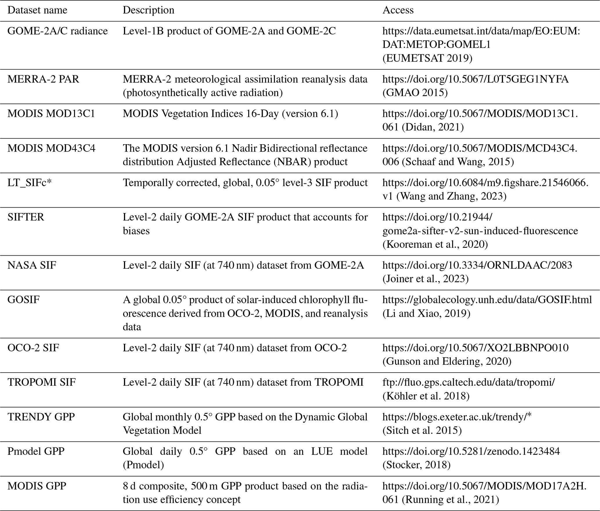
The NDVI (normalized difference vegetation index) and three global GPP products were utilized for validation purposes. We employed the global NDVI derived from the MOD13C1 product. The MOD17A2H GPP (MODIS GPP) product, with a spatial resolution of 500 m (Running et al., 2021), was mosaicked globally every 8 d during the 2007–2021 period. The global simulated GPP based on the LUE model (Pmodel GPP) is a daily product from 1982 to 2016 whose spatial resolution is 0.5° (Stocker et al., 2019). The monthly 0.5° GPP derived from the Dynamic Global Vegetation Model (DGVM) for 2007 to 2021 was also utilized (TRENDY GPP version 11) (Sitch et al., 2015). The temporal range, temporal resolution, and spatial resolution of these datasets are summarized in Table 1. All these products were resampled at a spatial resolution of 0.5° and a temporal resolution of 1 month to enable their comparison.
Table 1The GPP and NDVI datasets used in this study and relevant details about them.
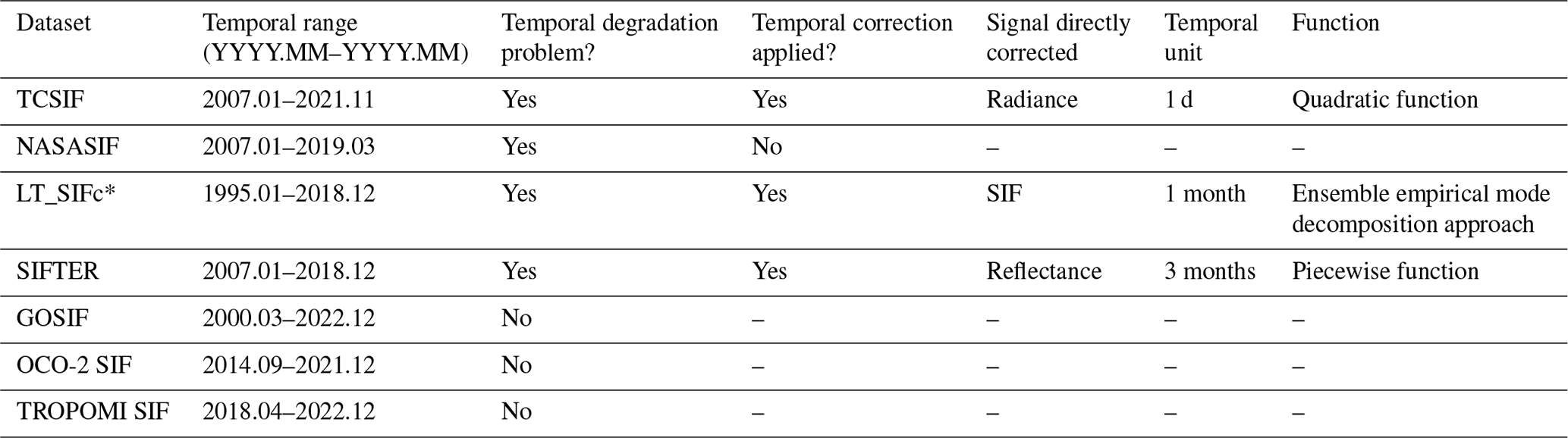
Next, we selected four long-term SIF products spanning more than 1 decade for comparison, including the LT_SIFc* (1995–2018) (Wang et al., 2022), SIFTER v2 (2007–2018) (van Schaik et al., 2020), GOSIF (2000–2022) (Li and Xiao, 2019), and GOME-2 SIF products generated by the National Aeronautics and Space Administration (hereon abbreviated to NASA SIF) (2007–2018) (Joiner et al., 2013, 2016). The LT_SIFc* is a data fusion product of GOME, SCIAMACHY, and GOME-2 with a spatial resolution of 0.05° and a temporal resolution of 1 month. It dealt with the temporal decay of the instrument based on statistics of the SIF signals in the Sahara. The SIFTER v2 product is the point-by-point SIF product retrieved from GOME-2 measurements after applying a time-related correction factor; it was composited to yield a monthly 0.5° global map in this study. The GOSIF product is the spatiotemporal extrapolation product based on the global neural network model and the OCO-2 SIF V8r product, with a spatial resolution of 0.05° and a temporal resolution of 8 d. Apart from the SIF products spanning decades, the OCO-2 SIF product from 2015 to 2021 and the TROPOMI SIF from 2018 to 2021 are also included here for comparative purposes due to their high accuracy and because they are less affected by sensor degradation. All SIF products were resampled to 0.5° spatial and monthly temporal resolution and were compared with TCSIF to assess long-term trends in this study. Additionally, we used the NASA GOME-2A level-2 SIF product, which has not been corrected for temporal decay, to verify the spatial distribution of our product. Key information about these SIF products is presented in Table 2.
Table 2The SIF products used in this study and relevant details about them. This information includes the temporal range of the dataset, whether the dataset initially had a temporal degradation problem, and, if so, whether the degraded dataset was corrected. The signal to which the correction factor is directly applied, the temporal unit of the correction factor, and the function describing the temporal correction are provided as well.
3.1 Pseudo-invariant method for calibrating the GOME-2A degradation
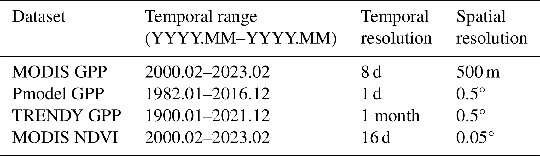
A homogeneous square region in the Sahara (22.5–23.5° E, 28.5–29.5° N; Fig. 1b) was selected as a pseudo-invariant site for calibrating the GOME-2A degradation. Ignoring the spatiotemporal variation in the far-red surface reflectance and atmospheric optical properties over the calibration site during the 2007–2021 period, the temporal trend in TOA GOME-2A reflectance could be deemed equivalent to the amount of temporal degradation in the GOME-2A instrument.
The MCD43C4 product was used here to investigate the homogeneity and stability of this calibration site. Figure 1b depicts the MCD43C4 surface reflectance and its spatiotemporal variance for the calibration site in 2007–2021. These results indicate that this site is bright (the near-infrared (NIR) reflectance is high, at 55.3 %–60.6 %), homogeneous (mean spatial variation = 0.29 %), and stable (with very low temporal variation of 0.81 %). Arguably, this site qualified as an ideal calibration site for implementing the pseudo-invariant method.
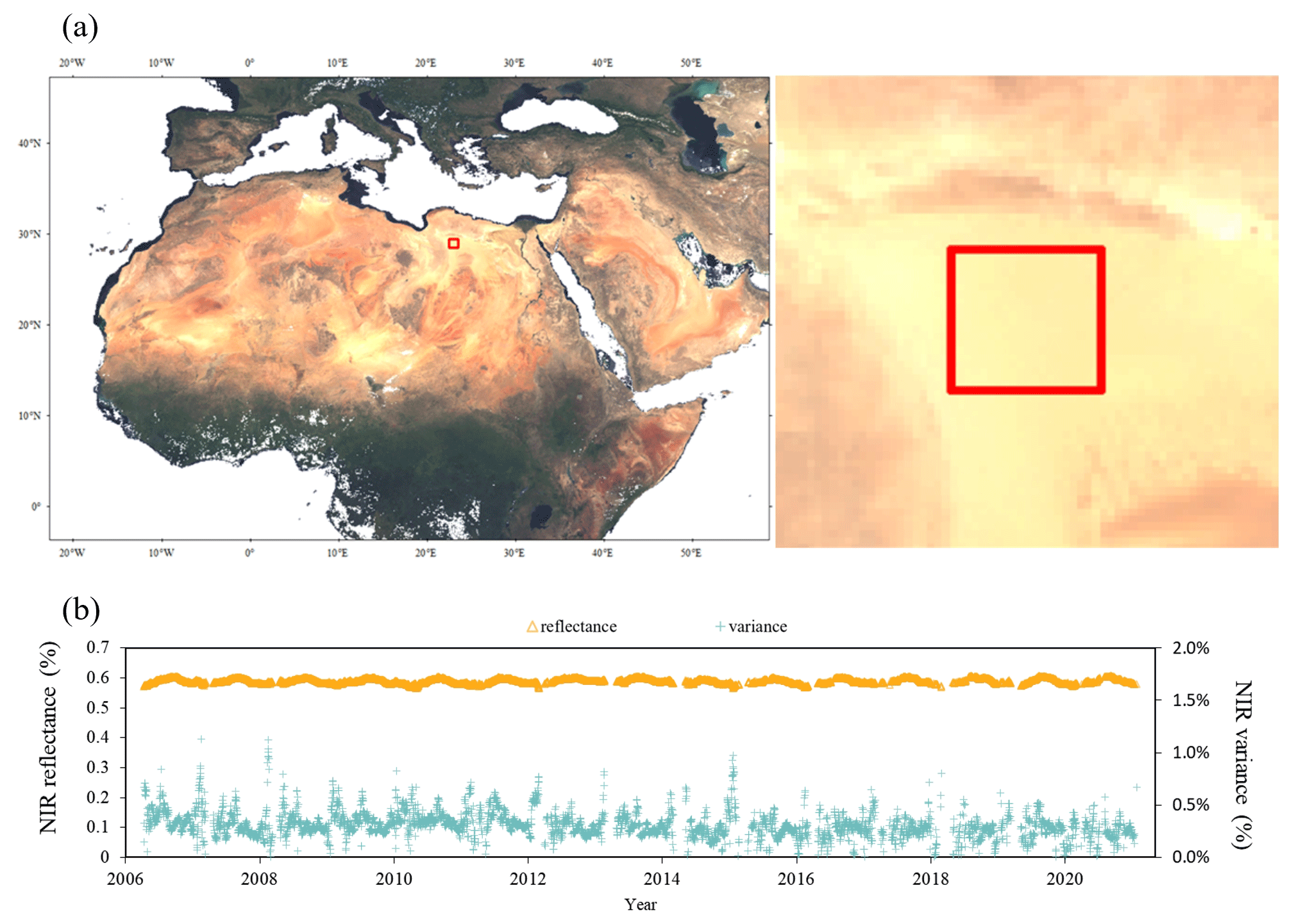
Figure 1(a) Location of the calibration site. (b) The NIR surface reflectance and its temporal variance at the calibration site (22.5–23.5° E, 28.5–29.5° N) during the 2007–2021 period. The NIR reflectance (shown by yellow triangles) and the NIR variance (shown by blue crosses) are, respectively, the mean and variance of the surface reflectance at the near-infrared band.
The clear-sky GOME-2A level-1B radiance products for the calibration site during 2007–2021 were downloaded to derive the temporal degradation. Two selection criteria for the GOME-2A data were applied: (1) a scanning angle of <20° and (2) no cloud contamination. This resulted in a total of 6885 GOME-2A level-1B radiance spectra being collected to correct for the GOME-2A degradation.
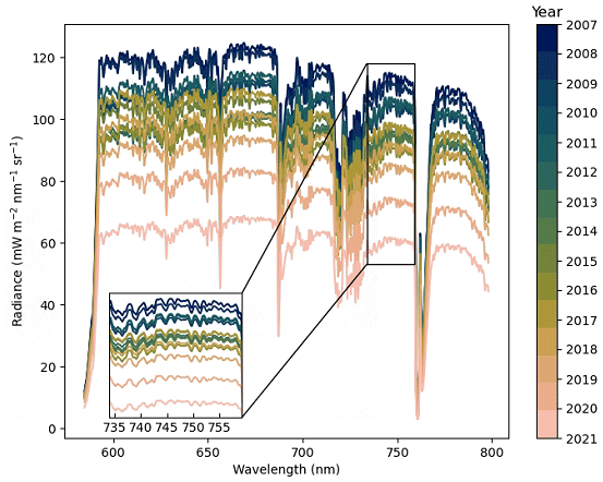
Figure 2Temporal variation in the GOME-2A level-1B top-of-atmosphere (TOA) radiance spectra at the calibration site (22.5–23.5° E, 28.5–29.5° N) for the 2007–2021 period. Different colors represent different years from 2007 to 2021.
Figure 2 depicts the yearly averaged TOA radiance spectra over the calibration site for each year in 2007–2021. Temporal degradation was determined using GOME-2A level-1B radiance products in the near-infrared (NIR) band between 735 and 758 nm, which served as the fitting window for SIF retrieval. Evidently, there is pronounced temporal degradation in the radiance spectra. Thus, a time-dependent correction factor was calculated, and the temporal correction function was assumed to be a second-order polynomial as follows:
where Dfactor is the degradation correction factor describing the temporal degradation; NOD is the number of days elapsed since 1 January 1900, starting with 1; and a, b, and c are the fitting coefficients of the polynomial function based on the near-infrared radiance of the pseudo-invariant site. The detailed analysis can be found in Sect. 4.1.
Next, the GOME-2A radiance can be corrected by dividing the measured radiance signal by the Dfactor:
where Radc and Rado are, respectively, the corrected radiance and the original radiance without correction for the degradation; Dfactor is the degradation correction factor in Eq. (1), which is used to compensate for the GOME-2A instrument's degradation since 2007.
3.2 Data-driven-based SIF retrieval method
The TCSIF dataset was separated from far-red SIF and corrected radiance spectra in the 735–758 nm range by using an singular vector decomposition (SVD)-based data-driven approach, namely that proposed by Guanter et al. (2015).
The TOA radiance (LTOA) was modeled this way:
where LTOA is the TOA radiance at 735–758 nm, λ is the measured wavelength used to represent the low-frequency information on surface reflectance and atmospheric scattering, and vj is the jth singular vector derived from non-vegetated targets (referred to as training datasets) that describes the high-frequency information on solar irradiance and atmospheric transmittance. αi and βj are the coefficients of the polynomial and singular vectors, respectively; Fs is the SIF intensity at 740 nm; λ is the wavelength; np is the order of the polynomial; and npc is the number of singular vectors selected. Finally, is the effective upward transmittance estimated as follows (Köhler et al., 2015):
where is the effective two-way atmospheric transmittance derived by normalizing the TOA reflectance using the low-order polynomial function; θ0 and θv denote the solar zenith angle and viewing zenith angle, respectively.
3.3 Post-processing of SIF retrieval results
The following quality-filtering criteria were applied (Guanter et al., 2012):
-
The land-cover type was set to vegetation.
-
The range of the mean radiance within the 735–758 nm window was between 25 and 200 mW m−2 nm−1 sr−1.
-
The absolute value of SIF was <5 mW m−2 nm−1 sr−1.
-
The solar zenith angle was <75°.
-
χ2 was <2.
Here, χ2 is the reduced chi-square value calculated based on the residuals from fitting (Sun et al., 2018), which characterizes the fit between the modeled and measured radiance using the forward model described above in Eq. (3). It is calculated as follows:
where Rad and Rad denote the ith spectral point of the modeled and measured radiance within the fitting window, respectively; “noise” denotes the random noise spectra; nf is the degrees of freedom; and nwi is the number of bands within the fitting window.
Also, we dealt with the effect of a zero-offset error in the SIF retrievals. Both the nonlinear response of the spectrometer radiance signals and the SVD data-driven algorithm can inevitably introduce systematic biases into the SIF retrieval results, especially in non-vegetated areas. Previous studies have identified systematic biases in SIF retrievals that depend on either the TOA radiance (Frankenberg et al., 2011; Guanter et al., 2012; Sun et al., 2017, 2018) or the latitude (Köhler et al., 2015; Joiner et al., 2016; van Schaik et al., 2020). Here we corrected the systematic biases (bias) by considering the radiance at the 735–758 nm window (Rad), the latitude (lat), and the observation zenith angle (θ0) of each footprint as follows (Joiner et al., 2016):
where A to H are the correction factors. These factors were first determined using the training dataset (where SIF is supposed to be zero and the retrieved SIF can be taken as the “bias”), which has a uniform latitude dimension, by applying the least-squares model. Next, the bias was calculated and subtracted from the SIF retrievals for each pixel.
3.4 Evaluation of the product accuracy
First, the root mean square of the model residual (rms_residual) was used to assess the accuracy of the data-driven model used to fit the radiance spectra. The model residual (Res) is the difference between the modeled and measured radiance:
where Rad and Rad denote the modeled and measured radiance spectra, respectively.
Second, the covariance matrix Se of the least squares for the SIF retrieval was calculated to assess the precision of the SIF retrievals:
where K is the Jacobian matrix formed by those linear model parameters from Eq. (3), and “noise” refers to the spectrally uncorrelated noise, which was calculated here based on the radiance and signal-to-noise ratio.
The standard error of the weighted mean (σSIF) within each grid cell was calculated in the following way (Du et al., 2018):
where σi is the 1σ error, which is the diagonal element of Se corresponding to Fs, and n is the number of sample points within each grid cell.
3.5 Upscaling the instantaneous SIF to the monthly averaged value
In previous studies, the global satellite-observed SIF was upscaled to a daily scale by using the diurnal cycle of the cosine of the solar zenith angle (cos [SZA]) to correct for day-length effects (Frankenberg et al., 2011; Zhang et al., 2018). These effects can cause large overestimates of SIF on cloudy days because the satellite-observed SIF data are only available on clear-sky days. In this study, the downwelling PAR rather than cos (SZA) was used to compensate for the significant effects of diurnal weather changes due to cloud and atmospheric scattering (Hu et al., 2018) while upscaling the instantaneous SIF to monthly values. The all-sky monthly averaged SIF (SIFmon) can be determined using the PAR-based upscaling model as follows:
where SIFins is the GOME-2A level-2 daily instantaneous clear-sky (i.e., <30 % cloud fraction) SIF, the terms PARmon and PARins are the corresponding monthly and instantaneous values of PAR, and EVImon and EVIins are the respective monthly and daily EVI values. M is the number of valid measurements within the 0.5° grid cell during the relevant monthly period. The EVI is negligible if the EVI value for the cell is <0.2.
Based on the PAR-based upscaled model, the instantaneous GOME-2A SIF clear-sky observations with a correction for temporal degradation were upscaled to their monthly average values.
4.1 Correction of GOME-2A sensor degradation
A second-order polynomial was fitted to describe the temporal degradation in the reflectance signal of GOME-2A. Figure 3a illustrates the temporal variation in TOA reflectance at 758 nm at the calibration site. Significant and continuous degradation can be observed; however, this nonlinear trend was accurately captured by a quadratic polynomial function with a determination coefficient (R2) of 0.851. These results indicated that, overall, the GOME-2A instrument degraded by 16.21 % from 2007 to 2021. This temporal degradation was considered spectrally constant in the narrow fitting window of the SIF retrieval (735–758 nm).
By dividing the NIR reflectance by the value of the fitted function at the starting date (1 January 2007), we obtain the degradation factor (Dfactor), as shown in Fig. 3b. The second-order polynomial fit was used in Eq. (2) to calibrate the instrument's degradation since 1 January 2007, as given by
where NOD is the number of days since 1 January 1900.
The temporally corrected GOME-2A NIR radiance was validated using GOME-2C radiance spectra (Fig. 4). For the corrected GOME-2A radiance, the scatter plot shows that the majority of points are concentrated near the 1:1 line (Fig. 4a). The difference between the two products followed a Gaussian distribution with a small mean value of 1.85 mW m−2 sr−1 nm−1, which is 2.3 % of the mean GOME-2A radiance (Fig. 4b). In contrast, the mean deviation without temporal correction is 15.16 W m−2 sr−1 nm−1 (Fig. 4d). Slight positive offsets can be found in both linear regression results. The difference in orbit height between GOME-2A (827 km) and GOME-2C (817 km) leads to the difference in viewing zenith angle (VZA). Although only observations with VZA <20° were selected, and the effect of observing angle has been corrected for by dividing by the cosine of VZA, there may still be differences due to the anisotropy of the ground surface, which introduces systematic errors.
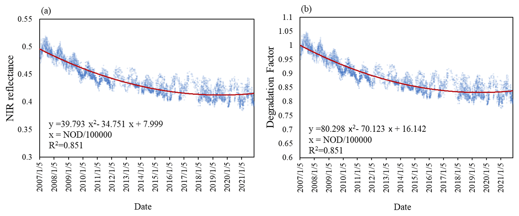
Figure 3Temporal variation in the TOA reflectance at 758 nm at the calibration site (a) and the temporal correction coefficients used to compensate for the degradation of GOME-2A since 2007 (b). The blue dots and red curves in (a) represent NIR reflectance and the fitted quadratic function, respectively. The degradation factor (Dfactor) in (b) was calculated by dividing the NIR reflectance by the value of the quadratic function in (a) at the starting date (1 January 2007). NOD in the degradation correction equation is the GOME-2A acquisition date since 2007, which equals the number of days from 1 January 1900.
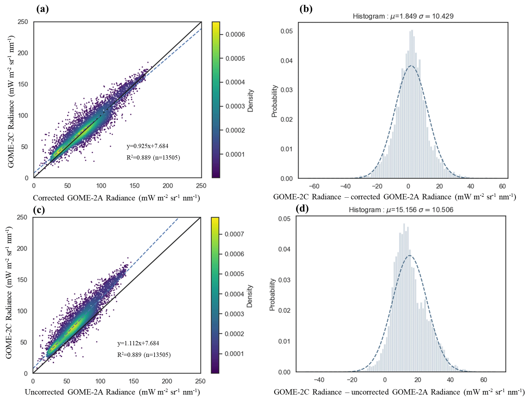
Figure 4Comparison between the GOME-2A and GOME-2C NIR radiance after (a, b) and before (c, d) the temporal correction on 1 July 2019. Histograms of the GOME-2C NIR radiance minus the corrected GOME-2A NIR radiance and the GOME-2C NIR radiance minus the uncorrected GOME-2A NIR radiance are shown in (b) and (d), respectively. Spatially matched pixels with a cloud fraction lower than 0.3, a VZA lower than 20°, and an SZA lower than 70° were selected.
4.2 Uncertainty of the data-driven algorithm
The fitting residual and single-retrieval error of the TCSIF dataset were analyzed to verify the feasibility of the data-driven retrieval algorithm as well as the quality control process.
As Fig. 5 shows, the fitted data-driven model described the measured radiance spectra well, with a root mean square (rms) of the residual that was below 0.30 %. The model that considers the fluorescence is more capable of reconstructing the radiance spectra than the model which ignores the fluorescence, as it has a slightly lower rms_residual (around 0.02 % on average).
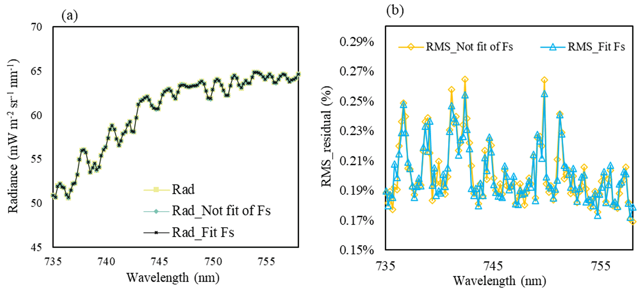
Figure 5(a) Radiance spectra in the 735–758 nm fitting window over vegetated areas on 15 July 2017: measured spectrum (Rad, represented by squares) and spectra that were modeled with (Rad_Fit Fs, represented by diamonds) and without (Rad_Not Fit of Fs, represented by crosses) accounting for SIF. (b) Root mean square (rms) values of the fitting residual obtained when SIF was (rms _Fit Fs, represented by yellow diamonds) and was not (rms_Not Fit of Fs, represented by blue triangles) accounted for. Each spectrum is the average of 224 vegetation spectra over pixels with a cloud fraction of <0.1 and a SIF intensity of >1.5 mW m−2 sr−1 nm−1.
4.3 Spatial distribution of the TCSIF dataset
Figure 6 shows the global pattern of monthly TCSIF in the summer and winter of 2008. The monthly GOME-2A SIF dataset captured the spatial pattern in both seasons well, with high SIF values present in Southeast Asia, the North American Corn Belt, and central Europe in July and the Amazon rainforest and most of South America in December. Crucially, the standard error of the weighted mean (σ(Fs)) is lower than 0.1 mW m−2 sr−1 nm−1 in most regions globally, while the main vegetated areas have σ(Fs) values lower than 0.05 mW m−2 sr−1 nm−1 (Fig. 6).
We also compared the spatially matched TCSIF and NASA SIF pixels in January and July 2008, July 2017, and January 2018 (Fig. 7a–d). The linear relationships between the two SIF products revealed that they were strongly correlated (R2>0.65), significant (p value <0.05), and close to the 1:1 correspondence line (slope >0.84) for both seasons in 2008 (Fig. 7a, b). For comparison, in 2017 and 2018 (Fig. 7c, d), there are still good linear relationships between TCSIF and NASA SIF (R2>0.64). However, it is worth noting that the regression line deviates from the 1:1 line in both 2017 and 2018 (slope <0.80), which is caused by the degradation in NASA SIF.
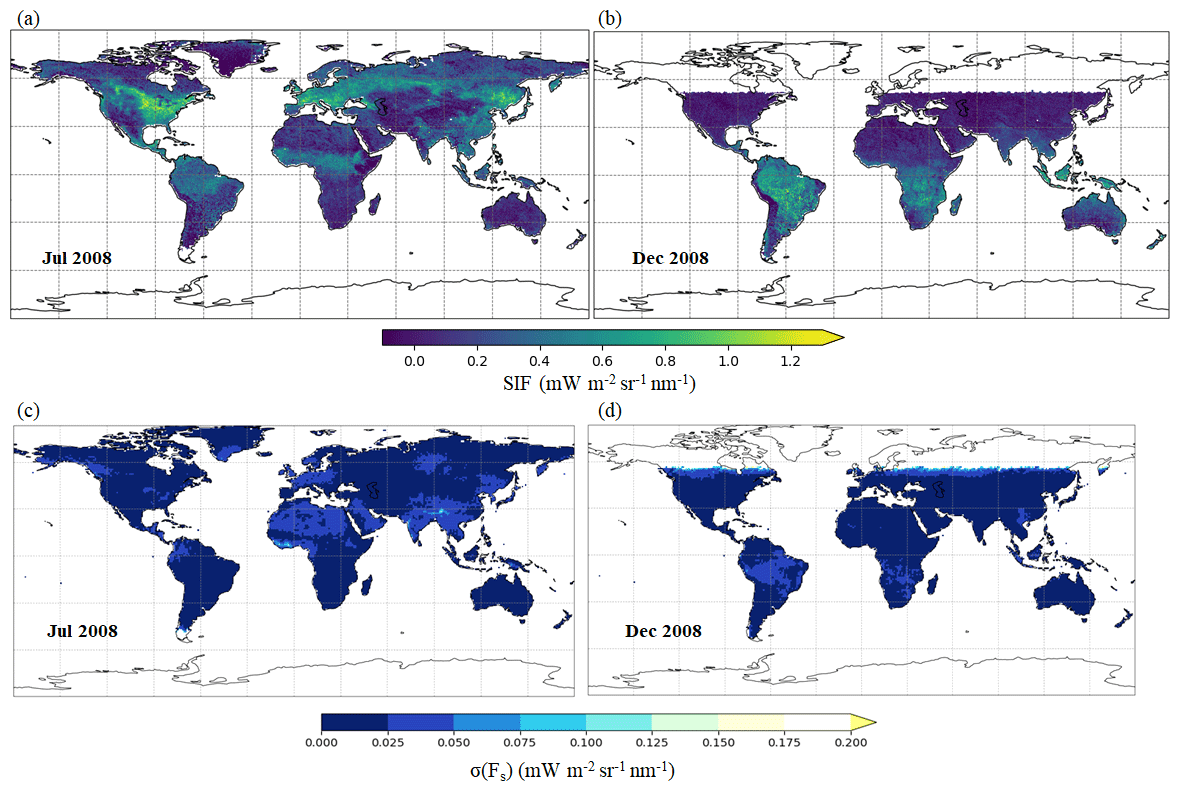
Figure 6Global patterns in the upscaled monthly TCSIF (a, b) and the standard error of the weighted mean (σ(Fs)) (c, d) in July (a, c) and December (b, d) in the year 2008.
OCO-2 SIF and TROPOMI SIF were also involved in the validation of TCSIF (Fig. 7e, f). To avoid discrepancies in wavelength and the overpassing time, the day-length-corrected 740 nm values provided by OCO-2 SIF, TROPOMI SIF, and TCSIF were compared. The spatially matched points were selected. TCSIF versus OCO-2 SIF and TCSIF versus TROPOMI SIF comparisons were conducted in July 2019 and July 2021, respectively. Both comparisons show high consistency, with R2>0.65, and the linear regression results are close to the 1:1 line.
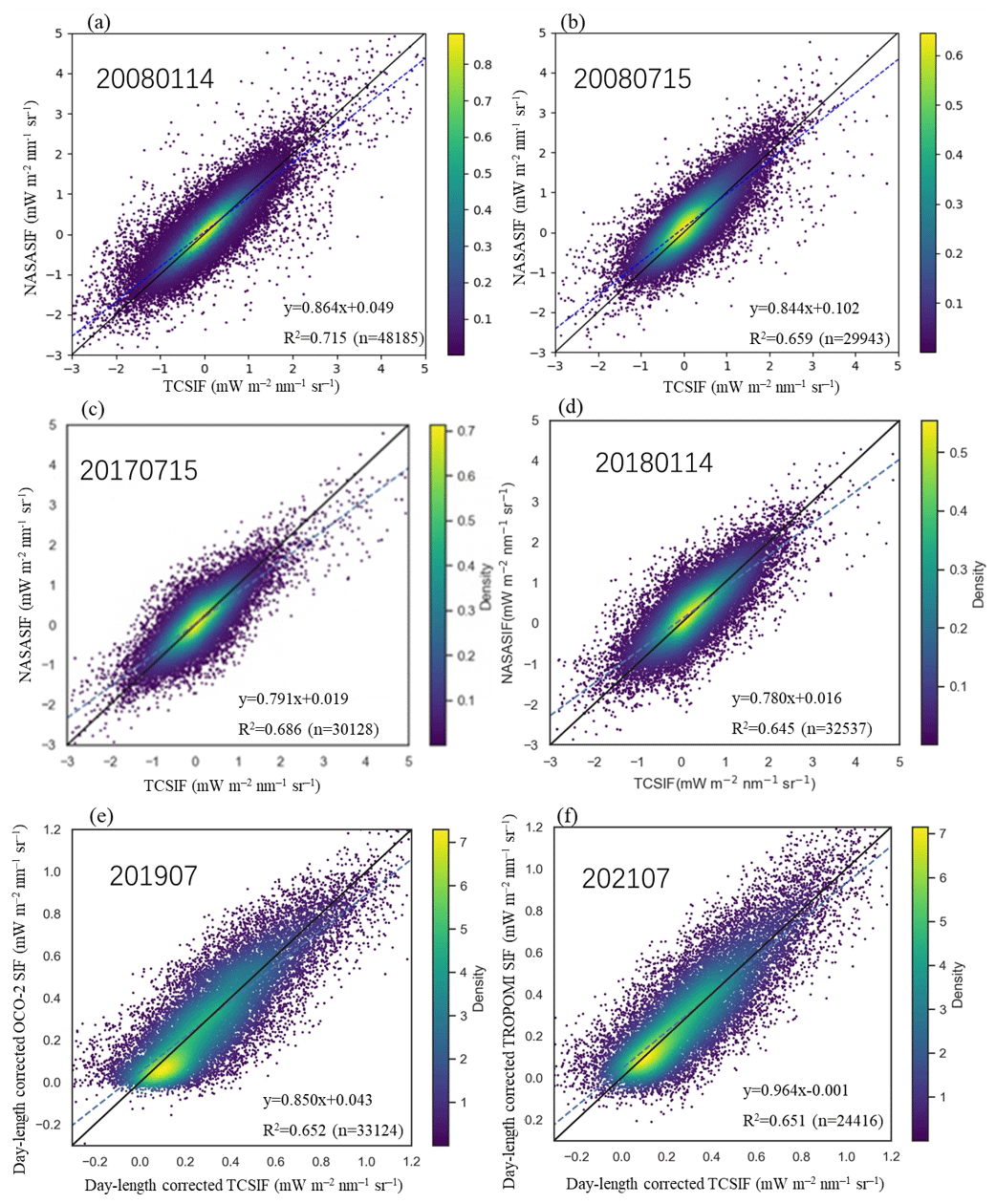
Figure 7Comparison of TCSIF vs. NASA SIF on 14 January (a) and 15 July (b) in the year 2008 and on 15 July 2017 (c) and 14 January 2018 (d). Comparisons of TCSIF versus OCO-2 in July 2019 (e) and TCSIF versus TROPOMI SIF in July 2021 (f). The comparisons were made based on the level-2 product. Co-located pixels over land with a cloud fraction <0.3 were selected. The color of the scatter points represents the density of the points. The dotted blue line and the solid black line represent the line fitted based on the scatter points and the 1:1 line, respectively.
4.4 Temporal variation in the TCSIF dataset
The global monthly SIF is averaged to demonstrate the temporal variation (Fig. 8). The autocorrelation coefficient of the time series is calculated for each pixel, and only the vegetation-covered pixels with an autocorrelation coefficient greater than 0.4 are selected to ensure the authenticity of the time series. Compared with the NASA SIF products, which gave a downward trend in SIF for 2007–2018, the global monthly mean trend in TCSIF exhibited an upward trend. The monthly trend in global averaged SIF shifted from a decrease of 1.15 % yr−1 to an increase of 0.71 % yr−1 after correcting for the instrument's degradation. As seen in Fig. 9, the trend in SIF variation was underestimated in almost all vegetation regions before the temporal correction, with the effect of the correction being particularly prominent at low latitudes in the Southern Hemisphere (0–20° S) as well as at middle and high latitudes in the Northern Hemisphere (30–70° N).
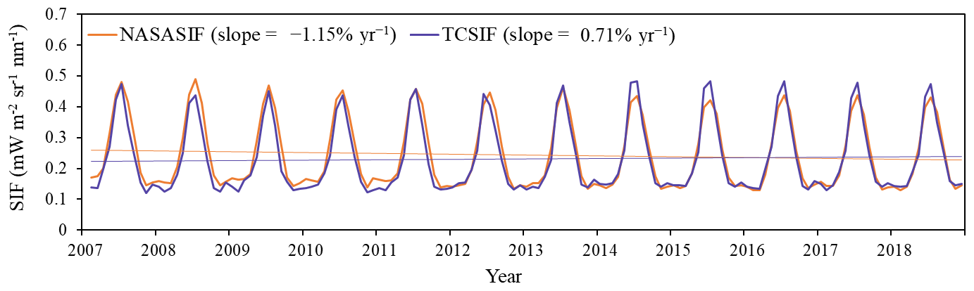
Figure 8Time series of the monthly averaged global GOME-2A SIF for 2007–2018 with (purple line) and without (orange line) the degradation correction. The daily level-2 NASASIF product was composited and filtered in the same way as for TCSIF.
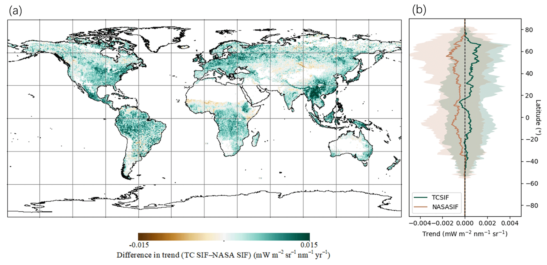
Figure 9(a) Difference in temporal trend between SIF products with and without temporal correction and (b) the latitudinal profiles of (a) for 2007–2018. The brown- and green-shaded areas in (b) represent the standard deviations of the TCSIF and NASA SIF trends, respectively.
The temporally consistent SIF dataset was then applied to reveal spatiotemporal patterns in the photosynthetic activity of global vegetation. Figure 10 shows the global patterns in the trends for the annual average TCSIF in the 2007–2021 period. When tallied, 62.91 % of the vegetated areas were distinguished by an upward trend in SIF, whereas 13.86 % corresponded to a significant increase over time (p<0.05). The regions that showed a significant increase in SIF were mainly located in Southeast Asia, eastern China, western Europe, central Africa, and South America. Only 4.51 % of the vegetated parts of the Earth's vegetated surface experienced a significant decrease in SIF.
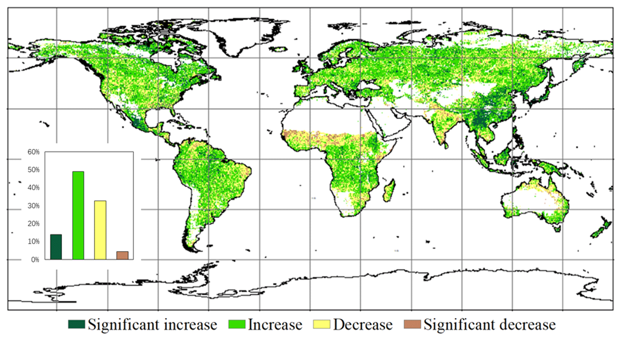
Figure 10Map of trends in the annual average GOME-2A SIF for 2007–2021. The inset shows the percentages of the area that were characterized by four types of trends: a significant increase (a positive correlation with p<0.05), an increase (a positive correlation with p≥0.05), a decrease (a negative correlation with p≥0.05), or a significant decrease (a negative correlation with p<0.05).
Figure 11Map of trends in the annual average (a) NASA SIF for 2007–2018, (b) OCO-2 SIF for 2015–2021, and (c) TRENDY GPP and (d) NDVI for 2007–2021. The colors represent four types of trends: a significant increase (a positive correlation with p<0.05), an increase (a positive correlation with p≥0.05), a decrease (a negative correlation with p≥0.05), or a significant decrease (a negative correlation with p<0.05).
As shown in Fig. 11, 57.11 % of the vegetated area is facing a decline in NASA SIF. In contrast, as seen from OCO-2 SIF, TRENDY GPP, and NDVI, vegetation was growing over a large area globally (>70 %) from 2007 (or 2015) to 2021. The main inconsistency between NASA SIF and the other products occurs in central and southern Africa, eastern Europe, and southern North America, where NASA SIF declines and the others increase. In southeastern China, vegetation greening was found by TCSIF, OCO-2 SIF, and NDVI, while an insignificant downward trend was shown by TRENDY GPP. Vegetation growth in southern North America, Europe, the Amazon rainforest, central Africa, and Southeast Asia was detected by all the products apart from NASA SIF.
5.1 Degradation at different locations and wavelengths
In this study, only one calibration site (Libya 4) was used for the fitting of the degradation function. The results may be different for different sites. Previous studies have compiled 20 pseudo-invariant calibration sites (PICSs) for instrument calibration (Cosnefroy et al., 1996; Bacour et al., 2019). We have involved three other commonly used sites, and the related information is shown in Table 3.
Table 3The four pseudo-invariant calibration sites (PICSs) and related information.
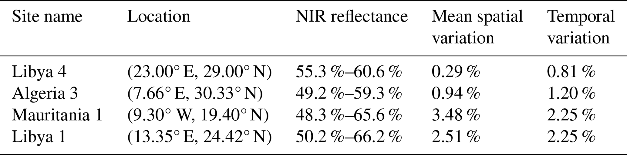
Among the four PICSs, Libya 4 was shown to be the best site for the calibration, as it is bright (the near-infrared (NIR) reflectance is high, at 55.3 %–60.6 %) and it is the most homogeneous (mean spatial variation = 0.29 %) and most stable (with a very low temporal variation of 0.81 %) site. On the other hand, similar interannual declining trends are given by the four PICSs (Fig. 12a). The NIR reflectances of Libya 4, Algeria 3, Mauritania 1, and Libya 1 declined by 16.21%, 17.57 %, 17.20 %, and 16.38 % from 2007 to 2021, respectively. Therefore, we can reliably fit the degradation of GOME-2A using the Libya 4 site only.
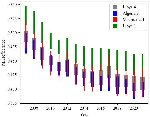
Figure 12Instrument degradation at the four different calibration sites. Each bar shows the yearly average ± standard deviation.
In addition, the degradation at different wavelengths may also differ. Degradation functions fitted by different wavelengths in the 735–758 nm were compared. A difference of less than 1 % was found when the degradation from 2007 to 2021 was fitted at different wavelengths (Fig. 13a and b). Figure 13b shows the variation in the temporal decay at different wavelengths and indicates that inconsistency mainly occurs at the Fraunhofer line, which is inherently unstable over time. On the other hand, SIF retrieval relies on the fitting of absorption lines. Extremely high fitting accuracy must be ensured if the wavelength is considered to be a factor that influences the degradation function; otherwise, the accuracy of SIF retrieval will be greatly affected. Therefore, in this study, the wavelength dependence of the degradation within the 735–758 nm window is ignored.
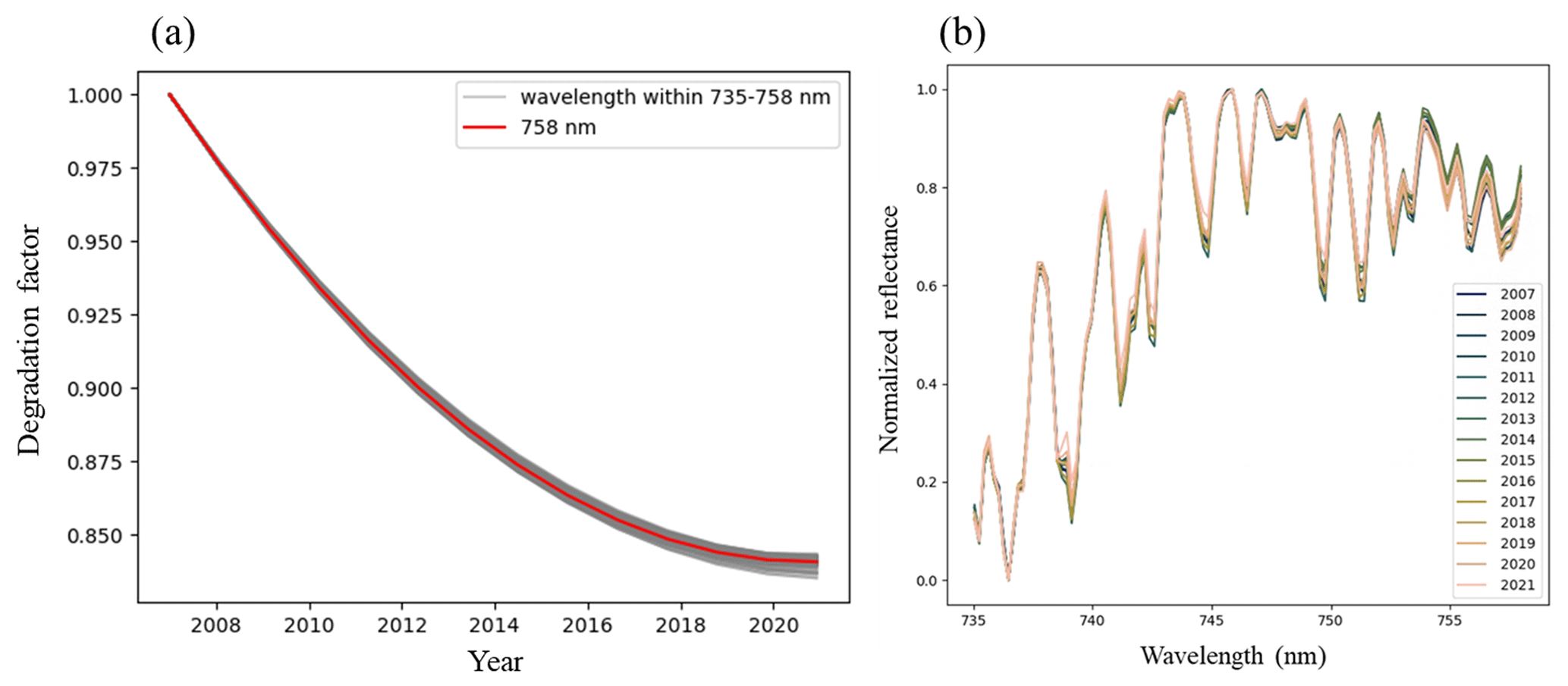
Figure 13(a) The degradation factor (Dfactor) fitted using the reflectance at different wavelengths in the 735–758 nm fitting window. The red line is the result obtained at 758 nm, while the degradation functions fitted by other wavelengths are shown in gray. (b) Normalized NIR reflectance spectra in the 735–758 nm fitting window for different years from 2007–2021.
5.2 Uncertainty in the temporal correction method
A wide range of radiance is essential for ensuring the representativeness of the temporal correction function, since the degradation may differ across different radiance levels. Although the pseudo-invariant sampling region selected in this study has a small spatial extent, it has a large radiance range (48–284 mW m−2 sr−1 nm−1) which almost covers that of the main vegetated areas at the near-infrared band (Fig. 14); only the lowest value of vegetation radiance (24 mW m−2 sr−1 nm−1) is not covered. Since temporal invariance is required for the calibration site, it leaves a few optional samples to choose from. The representativeness of samples may have an impact on the correction coefficient.
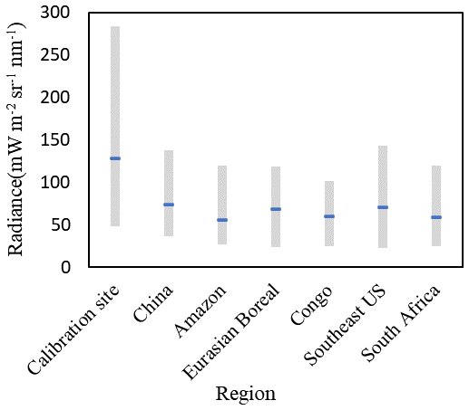
Figure 14Range of radiance at the near-infrared band at the calibration site and in the six main vegetated areas. The gray bars and blue lines are the range and mean of the datasets, respectively.
The relative residuals of the corrected GOME-2A NIR radiance at vegetated targets under different radiance levels were analyzed. As shown in Fig. 15, the relative residuals are less than 20 % when the NIR radiation is greater than 25 mW m−2 sr−1 nm−1, and the averages of the relative residuals are less than 7 %. The results indicate that the correction is essentially accurate at different radiance levels. However, when the radiance is lower than 25 mW m−2 sr−1 nm−1, the relative residual error reaches 40%. One reason for this result is that low radiance signals are greatly affected by random noise, resulting in poor comparability of GOME-2A and GOME-2C. Also, the extremely low radiance level cannot be estimated using the correction based on desert pixels. Therefore, the correction results can be inaccurate for pixels with low vegetation coverage or stressed vegetation.
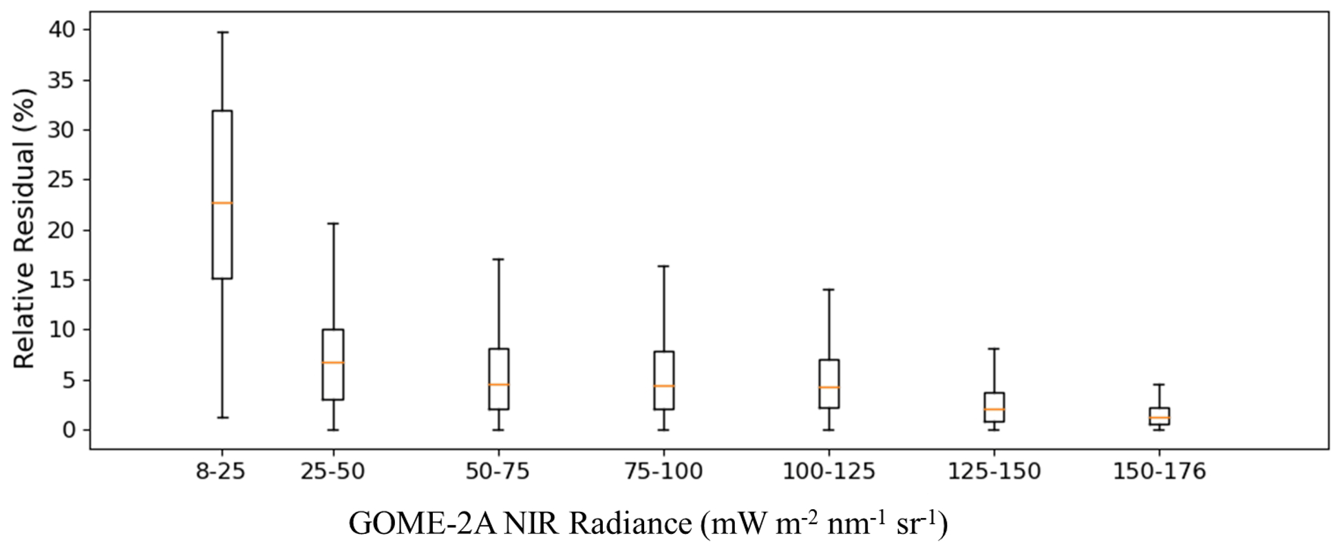
Figure 15Relative residual of the NIR radiance (calculated as the absolute difference between the GOME-2A and GOME-2C NIR radiance at the co-located points) at different radiance levels. Global vegetation targets with SIF signals greater than 0.1 mW m−2 sr−1 nm−1 on 1 July 2019 were selected.
Another limitation is that we only indirectly verify the reliability of the interannual trend of TCSIF when using several long-term remote-sensing products, such as GPP, NDVI, and other SIF products. Direct validation data, such as field measurements, were not used to prove the accuracy of our results. In this respect, the huge discrepancy in scale between the satellite SIF products (0.5°) and ground observations (<100 km2) is one of the major obstacles. In fact, to our best knowledge, there is no available decade-long in situ SIF validation dataset that is sufficiently reliable for such a direct validation, and the methodology of directly verifying satellite SIF based on in situ measurements is still imperfect (Parazoo et al., 2019). The accuracy of TCSIF products needs to be verified via future applications.
The contamination of the lens may not be the only reason for GOME-2A's degradation. As shown in Fig. 3, the intra-annual variation in NIR reflectance does not decrease, unlike the interannual average. Instead, the intra-annual variation grows with time. A similar phenomenon was found in the chlorine dioxide products (Pinardi et al., 2022): the GOME-2A results are noisier than those of GOME-2B, especially after 2011. These results suggest that, in addition to the decline in reflectance over time caused by lens contamination, the temporal degradation impacts GOME-2A measurements in other forms. However, the pattern of this effect is not yet clear; further research is needed on more aspects of the impact of GOME-2A's degradation on its measurements. Therefore, only the interannual declining trend was considered in this study, while the inevitable intra-annual variations caused by other factors such as the bidirectional reflectance distribution function and atmospheric scattering were neglected.
5.3 Comparison with other long-term SIF products
The annual average values of TCSIF and other long-term SIF products were compared (Fig. 16). Importantly, most of the long-term SIF products were in agreement and featured an increasing trend in SIF from 2007 to 2018, except for NASA SIF and SIFTER (Fig. 16a–e). Among the temporally corrected SIF products, the annual curves of TCSIF and LT_SIFc* are generally consistent, while LT_SIFc* gives a more strongly increasing trend of 1.247% yr−1, and the uncertainty of the growing trend in TCSIF (0.15 % yr−1) is lower. A slightly decreasing trend of −0.08 % yr−1 characterized the SIFTER v2 product (Fig. 16b), while the annual fluctuation in SIFTER v2 was clearly the greatest among all the SIF products shown in Fig. 16 (0.37 % yr−1). The yearly trend according to TCSIF (1.06 % yr−1) is close to the results from OCO-2 SIF for 2015 to 2021 (1.23% yr−1; Fig. 16f), while GOSIF shows a slower growing trend of 0.50% yr−1 during the same period. Compared to GOSIF, which was derived from OCO-2 SIF using a machine-learning method, TCSIF is even more consistent with OCO-2 SIF, suggesting that machine-learning methods have flaws in relation to maintaining the temporal trend of the original SIF products.
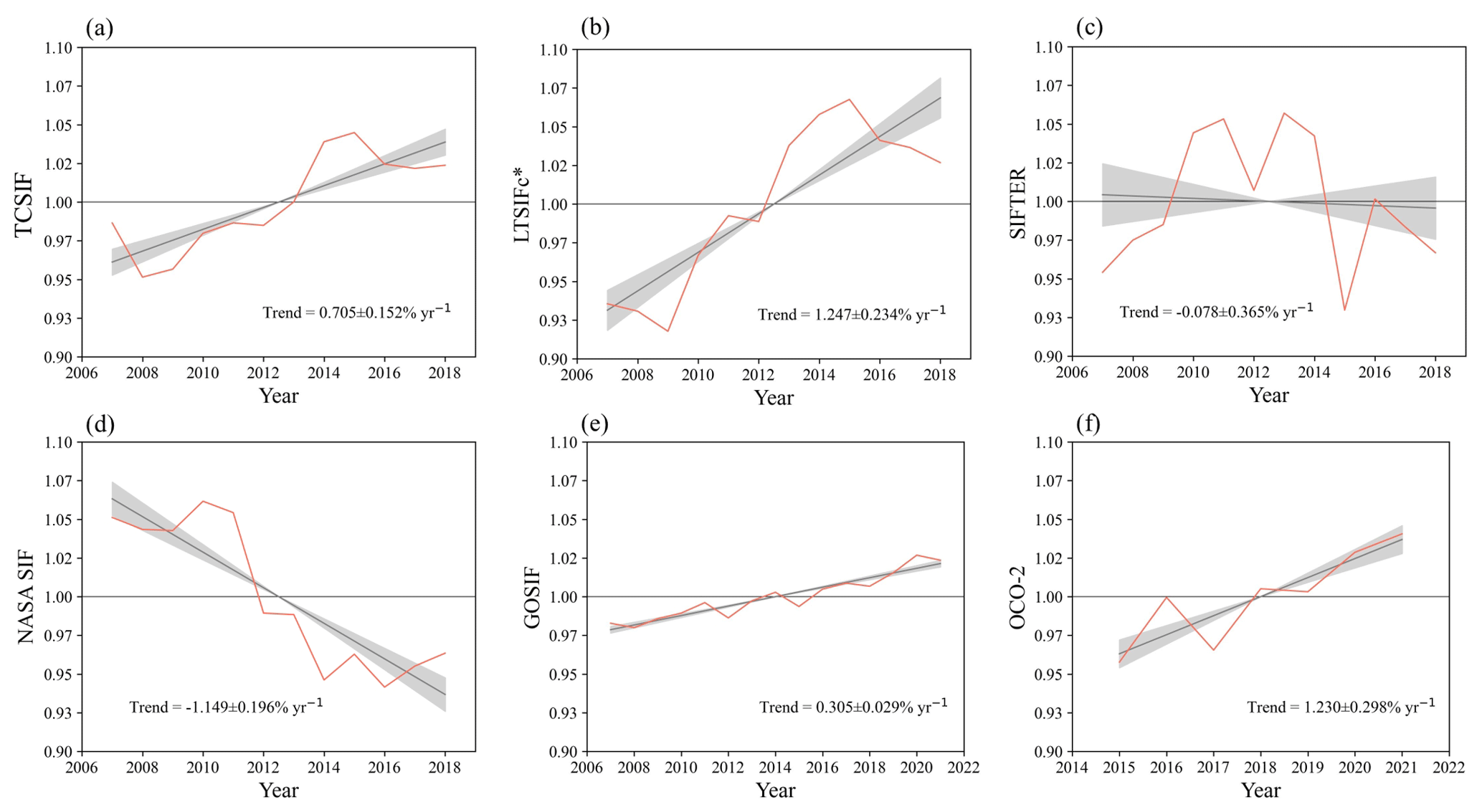
Figure 16Comparison of temporal trends in the annual SIF average from (a) TCSIF, (b) LT_SIFc*, (c) SIFTER v2, and (d) NASA SIF during 2007–2018, from (e) GOSIF during 2007–2021, and from (f) OCO-2 SIF during 2015–2021. All data shown are normalized to relative values (by dividing by the mean). The shaded areas indicate the standard deviations.
The large interannual fluctuation of SIFTER may be caused by the fact that its correction factor is seasonally based. No continuous correction functions were applied by SIFTER, which runs counter to the sensor's general pattern of temporal decay (Lyapustin et al., 2014; Wang et al., 2012). In stark contrast, the least interannual fluctuation was found in the GOSIF product. A neural network model was used for the spatiotemporal degradation of the GOSIF product, enabling GOSIF to inherit the time-stable signal from MODIS reflectance. However, this neural network model has been criticized for relying too much on training data, such as reflectance data, and overlooking valuable information in the original observations (Ma et al., 2020). In the years not covered by the original OCO-2 SIF, the spatial distribution of GOSIF depends almost entirely on other input parameters of the data-driven model; hence, it cannot reliably capture the long-term temporal trend in SIF.
The LT_SIFc* product uses weak SIF signals over the Sahara to fit the temporal decay pattern of the sensor, which can quickly generate corrected SIF products based on the monthly global maps provided by NASA SIF. Nevertheless, the method is not rigorous enough, since the sensor's degradation does not alter the SIF retrievals in a linear way. The post-processing steps, such as the zero-offset correction and quality-filtering procedures, will influence the distribution of global gridded SIF products, leading to uncertainties in the correction function. Besides this, a large proportion of noise signals accompany the weak SIF signals over desert targets, thus restricting the fitting accuracy of the corrective function. Meanwhile, LT_SIFc* is obtained by fusing three SIF products using the cumulative distribution frequency (CDF)-matching approach. Accordingly, the spatiotemporal distribution of the original SIF signal may be forced to change due to adjustments in the distribution frequency of each separate product. In this study, we corrected the degradation in radiance spectra rather than the SIF by using pseudo-invariant pixels over the Sahara, which should provide a more reliable method.
To take advantage of SIF's ability to capture rapid changes in GPP, the temporal resolution of long-term SIF products needs to be higher than 1 month or even a few days (Zhang et al., 2014, 2016; Porcar-Castell et al., 2014). However, LT_SIFc* cannot meet these temporal resolution requirements as it is constrained by the original SIF products. By contrast, the shorter repeating cycle of GOME-2 was fully utilized in this study. Our work provides global daily level-2 SIF products that encompass the world's terrestrial area, which will greatly improve the applicability of global SIF products to the monitoring of global vegetation dynamics.
5.4 Interannual trends for the TCSIF, NDVI, and GPP products
We compared the interannual trend in TCSIF with those of GPP and NDVI. Parameter values during the peak of the growing season were compared to show the period when the vegetation was most lush each year. After the spatial averaging of monthly products, the yearly annual maximum values were calculated year by year.
As evinced by Fig. 17a–e, the global yearly maximum TCSIF showed a trend of increasing SIF intensity, which was consistent with those of GPP and NDVI. The interannual fluctuation of TCSIF (0.16 %) slightly exceeded those of the GPP and NDVI products (both <0.1 % yr−1) during the 2007–2021 period, and likewise for 2007–2016. The interannual trend and associated uncertainty of each product are displayed in Fig. 17f. Given that the time span of Pmodel GPP stops at 2016, we selected the NDVI and TCSIF series from 2007 to 2016 for a fair comparison with Pmodel GPP; this is shown in the bottom half of Fig. 17f. Evidently, there are deviations between the interannual vegetation growth trends inferred from different GPP products. For example, from 2007 to 2021, the interannual growth trend estimated by MODIS GPP (0.64 %) surpassed that of TRENDY GPP (0.44 %). Meanwhile, the interannual growth rate of TCSIF was close to those of MODIS GPP and Pmodel GPP in 2007–2021 and 2007–2016, respectively. Notably, when compared with the reflectance-based NDVI, the trend in TCSIF was more similar to that in GPP in both periods examined, indicating that TCSIF was more capable of tracking GPP than NDVI.
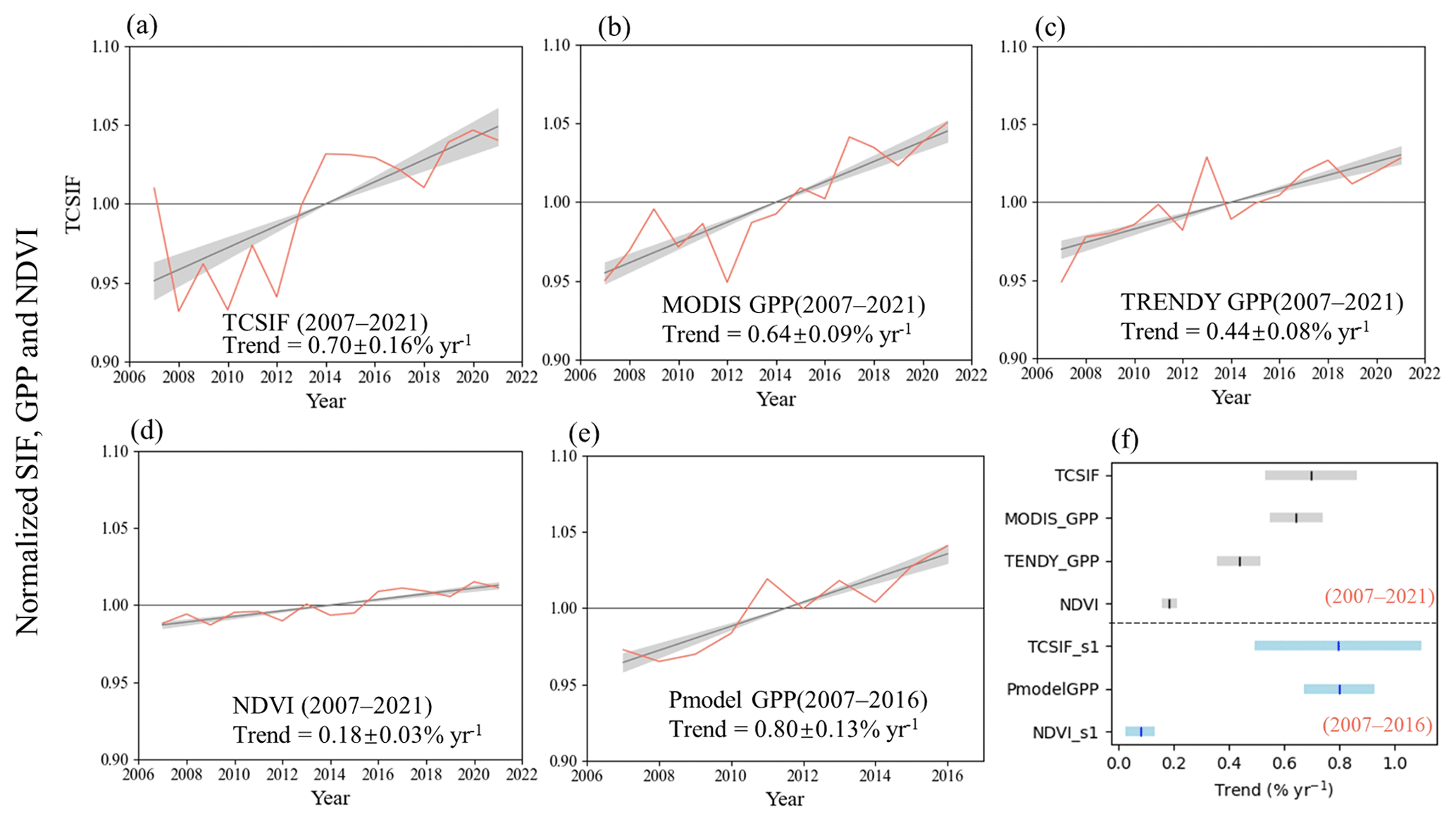
Figure 17Comparison of temporal trends in the yearly maximum from (a) TCSIF, (b) TRENDY GPP, (c) Pmodel GPP, (d) MODIS GPP, and (e) NDVI. All data shown are normalized to relative values (by dividing by the mean). The shaded areas indicate the standard deviations and the gray lines represent the fitted lines which show the general trends. The interannual trends (shown by the short vertical gray or blue lines) of all the products and their uncertainties (shown by the horizontal blue or gray bars) are shown in (f). TCSIF_s1 and NDVI_s1 correspond to the TCSIF and NDVI series for 2007–2016.
The global monthly GOME-2A SIF dataset (2007–2021) with the correction of temporal degradation is openly available at https://doi.org/10.5281/zenodo.8242928 (Zou et al., 2023; see Table A1 for access to other related datasets). The corrected global GOME-2 SIF dataset can be obtained in two forms. The daily level-2 dataset is provided in hdf5 format. The names of these files are given as SIF_daily_YYYYMMDD.h5, in which “YYYY”, “MM”, and “DD” denote the year, month, and date, respectively. The level-3 datasets, which were aggregated monthly from the level-2 dataset, have a spatial resolution of 0.5° and are saved in TIFF format in chronological order from 2007 to 2021. The names of these files are given as SIFpar_evi_monthly _YYYYMM.tif, in which “SIF” is the product type; “par” and “evi” represent upscaled parameters; “monthly” denotes the temporal scale, and “YYYY” and “MM” are the year and month, respectively. The SIF output is stored in the hdf5 files along with other variables of interest for further processing and visualization. See Appendix B for the structure of the hdf5 file.
Degradation of the GOME-2A instrument has been a major barrier to producing consistent SIF products over an extended time period. By normalizing the instrument's degradation from 2007 to 2021, the radiance spectra of GOME-2A were successfully corrected. The calibrated GOME-2A NIR radiance was shown to be accurate by comparing it to GOME-2C; the mean bias is 1.85 mW m−2 sr−1 nm−1. Based on the calibrated radiance, we were able to develop a temporally consistent SIF (TCSIF) dataset spanning decades for use in research. The TCSIF is strongly correlated with the NASA SIF, OCO-2 SIF, and TROPOMI SIF products in terms of its spatial distribution (R2>0.65), and it has a low retrieval residual (the rms of the residual is under 0.30 %). Our findings reveal that the TCSIF product yields a more reliable trend in vegetation SIF than the GOME-2A dataset without the degradation correction does. After undergoing the temporal correction, the vegetation SIF increased by 0.70 % per year during the 2007–2021 period, and 62.91 % of the global vegetated regions saw an increase in their SIF, suggesting an overall increase in vegetation SIF and photosynthesis during the growing season. Compared with NDVI, the results obtained by TCSIF are closer to the GPP, indicating that the TCSIF product is a reliable proxy for vegetation activity.
We conclude that the TCSIF product developed in this study represents a significant advancement in our ability to accurately assess long-term changes in the SIF of vegetation on a global scale. This product can thus serve as a valuable reference for past and future studies of long-term SIF products and may provide important insights into the impact of climate change on vegetation photosynthesis.
Table A1Access to the datasets used to generate and compared with TCSIF products.
* Last access: 1 July 2023. The information on data access can be found at https://globalcarbonbudgetdata.org/closed-access-requests.html (last access: 1 July 2023). The original TRENDY datasets can be requested from Stephen Sitch and Pierre Friedlingstein.
The fields of the level-2 products include the following.
-
SIF retrievals, including the instant SIF retrieved using the data-driven algorithm (SIF_740), the day-length-corrected SIF (SIF_daily), and the relative error estimations (the 1σ error (sigma_1), χ2, and the quality assurance field – QA).
-
Geolocations, which are fields that describe the location, including the latitude and longitude of the center and boundary of each footprint as well as the solar and viewing angles.
-
Ancillary data, including the reflectance at the red (ps_red) and far-red (ps_NIR) bands, the cloud fraction, the mean radiance in the 735–758 nm fitting window (Rad_NIR), and the NDVI calculated from the GOME-2 reflectance.
LL and XL designed the experiments, and CZ carried them out. CZ and SD developed the model code and generated the products. CZ prepared the manuscript with contributions from all co-authors.
The contact author has declared that none of the authors has any competing interests.
Publisher’s note: Copernicus Publications remains neutral with regard to jurisdictional claims made in the text, published maps, institutional affiliations, or any other geographical representation in this paper. While Copernicus Publications makes every effort to include appropriate place names, the final responsibility lies with the authors.
The authors acknowledge Philipp Köhler and Christian Frankenberg for publicly providing the TROPOMI SIF and OCO-2 SIF datasets. We acknowledge Stephen Sitch for sharing the link to the latest version of TRENDY GPP. Chu Zou acknowledges Songhan Wang for the instruction on the algorithm of LT_SIFc* data.
This work was supported by the National Key Research and Development Program of China (grant no. 2022YFB3904801) and the National Natural Science Foundation of China (grant nos. 42425001 and 42071310).
This paper was edited by Chaoqun Lu and reviewed by two anonymous referees.
Bacour, C., Briottet, X., Bréon, F.-M., Viallefont-Robinet, F., and Bouvet, M.: Revisiting Pseudo Invariant Calibration Sites (PICS) Over Sand Deserts for Vicarious Calibration of Optical Imagers at 20 km and 100 km Scales, Remote Sensing, 11, 1166, https://doi.org/10.3390/rs11101166, 2019.
Chen, C., Park, T., Wang, X., Piao, S., Xu, B., Chaturvedi, R. K., Fuchs, R., Brovkin, V., Ciais, P., Fensholt, R., Tømmervik, H., Bala, G., Zhu, Z., Nemani, R. R., and Myneni, R. B.: China and India lead in greening of the world through land-use management, Nature Sustainability, 2, 122–129, https://doi.org/10.1038/s41893-019-0220-7, 2019.
Cosnefroy, H., Leroy, M., and Briottet, X.: Selection and characterization of Saharan and Arabian desert sites for the calibration of optical satellite sensors, Remote Sens. Environ., 58, 101–114, https://doi.org/10.1016/0034-4257(95)00211-1, 1996.
Didan, K.: MODIS/Terra Vegetation Indices 16-Day L3 Global 0.05Deg CMG V061, NASA EOSDIS Land Processes Distributed Active Archive Center [data set], https://doi.org/10.5067/MODIS/MOD13C1.061, 2021.
Du, S., Liu, L., Liu, X., Zhang, X., Zhang, X., Bi, Y., and Zhang, L.: Retrieval of global terrestrial solar-induced chlorophyll fluorescence from TanSat satellite, Sci. Bull., 63, 1502–1512, https://doi.org/10.1016/j.scib.2018.10.003, 2018.
EUMETSAT: GOME-2 Level 1B – Metop – Global, EUMETSAT [data set], https://data.eumetsat.int/data/map/EO:EUM:DAT:METOP:GOMEL1 (last access: 15 January 2024), 2019.
Frankenberg, C., Butz, A., and Toon, G. C.: Disentangling chlorophyll fluorescence from atmospheric scattering effects in O2 A-band spectra of reflected sun-light, Geophys. Res. Lett., 38, L03801, https://doi.org/10.1029/2010GL045896, 2011.
Frankenberg, C., O'Dell, C., Berry, J., Guanter, L., Joiner, J., Köhler, P., Pollock, R., and Taylor, T. E.: Prospects for chlorophyll fluorescence remote sensing from the Orbiting Carbon Observatory-2, Remote Sens. Environ., 147, 1–12, https://doi.org/10.1016/j.rse.2014.02.007, 2014.
Gelaro, R., McCarty, W., Suárez, M. J., Todling, R., Molod, A., Takacs, L., Randles, C. A., Darmenov, A., Bosilovich, M. G., Reichle, R., Wargan, K., Coy, L., Cullather, R., Draper, C., Akella, S., Buchard, V., Conaty, A., da Silva, A. M., Gu, W., Kim, G.-K., Koster, R., Lucchesi, R., Merkova, D., Nielsen, J. E., Partyka, G., Pawson, S., Putman, W., Rienecker, M., Schubert, S. D., Sienkiewicz, M., and Zhao, B.: The Modern-Era Retrospective Analysis for Research and Applications, Version 2 (MERRA-2), J. Climate, 30, 5419–5454, https://doi.org/10.1175/JCLI-D-16-0758.1, 2017.
Global Modeling and Assimilation Office (GMAO): MERRA-2 tavg1_2d_lfo_Nx:2d,1-Hourly, Time-Averaged, Single-Level, Assimilation, Land surface Forcings V5.12.4, Goddard Earth Sciences Data and Information Services Center (GES DISC), Greenbelt, MD, USA [data set], https://doi.org/10.5067/L0T5GEG1NYFA, 2015.
Guanter, L., Frankenberg, C., Dudhia, A., Lewis, P. E., Gómez-Dans, J., Kuze, A., Suto, H., and Grainger, R. G.: Retrieval and global assessment of terrestrial chlorophyll fluorescence from GOSAT space measurements, Remote Sens. Environ., 121, 236–251, https://doi.org/10.1016/j.rse.2012.02.006, 2012.
Guanter, L., Zhang, Y., Jung, M., Joiner, J., Voigt, M., Berry, J. A., Frankenberg, C., Huete, A. R., Zarco-Tejada, P., Lee, J.-E., Moran, M. S., Ponce-Campos, G., Beer, C., Camps-Valls, G., Buchmann, N., Gianelle, D., Klumpp, K., Cescatti, A., Baker, J. M., and Griffis, T. J.: Global and time-resolved monitoring of crop photosynthesis with chlorophyll fluorescence, P. Natl. Acad. Sci. USA, 111, E1327–E1333, https://doi.org/10.1073/pnas.1320008111, 2014.
Guanter, L., Aben, I., Tol, P., Krijger, J. M., Hollstein, A., Köhler, P., Damm, A., Joiner, J., Frankenberg, C., and Landgraf, J.: Potential of the TROPOspheric Monitoring Instrument (TROPOMI) onboard the Sentinel-5 Precursor for the monitoring of terrestrial chlorophyll fluorescence, Atmos. Meas. Tech., 8, 1337–1352, https://doi.org/10.5194/amt-8-1337-2015, 2015.
Gunson, M. and Eldering, A.: OCO-2 Level 2 bias-corrected solar-induced fluorescence and other select fields from the IMAP-DOAS algorithm aggregated as daily files, Retrospective processing V10r, Goddard Earth Sciences Data and Information Services Center (GES DISC), Greenbelt, MD, USA [data set], https://doi.org/10.5067/XO2LBBNPO010, 2020.
Hahne, A.: Investigation on GOME-2 throughput degradation, ESA, https://www-cdn.eumetsat.int/files/2020-04/pdf_gome_thru_deg_esa.pdf (last access: 1 July 2023), 2012.
Hu, J., Liu, L., Guo, J., Du, S., and Liu, X.: Upscaling Solar-Induced Chlorophyll Fluorescence from an Instantaneous to Daily Scale Gives an Improved Estimation of the Gross Primary Productivity, Remote Sensing, 10, 1663, https://doi.org/10.3390/rs10101663, 2018.
Joiner, J., Guanter, L., Lindstrot, R., Voigt, M., Vasilkov, A. P., Middleton, E. M., Huemmrich, K. F., Yoshida, Y., and Frankenberg, C.: Global monitoring of terrestrial chlorophyll fluorescence from moderate-spectral-resolution near-infrared satellite measurements: methodology, simulations, and application to GOME-2, Atmos. Meas. Tech., 6, 2803–2823, https://doi.org/10.5194/amt-6-2803-2013, 2013.
Joiner, J., Yoshida, Y., Guanter, L., and Middleton, E. M.: New methods for the retrieval of chlorophyll red fluorescence from hyperspectral satellite instruments: simulations and application to GOME-2 and SCIAMACHY, Atmos. Meas. Tech., 9, 3939–3967, https://doi.org/10.5194/amt-9-3939-2016, 2016.
Joiner, J., Yoshida, Y., Koehler, P., Frankenberg, C., and Parazoo, N. C.: L2 Daily Solar-Induced Fluorescence (SIF) from MetOp-A GOME-2, 2007–2018, ORNL DAAC, Oak Ridge, Tennessee, USA [data set], https://doi.org/10.3334/ORNLDAAC/2083, 2023.
Köhler, P., Guanter, L., and Joiner, J.: A linear method for the retrieval of sun-induced chlorophyll fluorescence from GOME-2 and SCIAMACHY data, Atmos. Meas. Tech., 8, 2589–2608, https://doi.org/10.5194/amt-8-2589-2015, 2015.
Köhler, P., Frankenberg, C., Magney, T. S., Guanter, L., Joiner, J., and Landgraf, J.: Global retrievals of solar‐induced chlorophyll fluorescence with TROPOMI: First results and intersensor comparison to OCO‐2, Geophys. Res. Lett., 45, 10456–10463, https://doi.org/10.1029/2018GL079031, 2018 (data available at: ftp://fluo.gps.caltech.edu/data/tropomi/, last access: 15 January 2024).
Kooreman, M. L., Boersma, K. F., van Schaik, E., van Versendaal, R., Cacciari, A., and Tuinder, O. N. E.: SIFTER sun-induced vegetation fluorescence data from GOME-2A (Version 2.0), Royal Netherlands Meteorological Institute (KNMI) [data set]., https://doi.org/10.21944/gome2a-sifter-v2-sun-induced-fluorescence, 2020.
Koren, G., van Schaik, E., Araújo, A. C., Boersma, K. F., Gärtner, A., Killaars, L., Kooreman, M. L., Kruijt, B., van der Laan-Luijkx, I. T., von Randow, C., Smith, N. E., and Peters, W.: Widespread reduction in sun-induced fluorescence from the Amazon during the 2015/2016 El Niño, Philos. T. Roy. Soc. B, 373, 20170408, https://doi.org/10.1098/rstb.2017.0408, 2018.
Li, X. and Xiao, J.: A Global, 0.05-Degree Product of Solar-Induced Chlorophyll Fluorescence Derived from OCO-2, MODIS, and Reanalysis Data, Remote Sensing, 11, 517, https://doi.org/10.3390/rs11050517, 2019 (data available at: https://globalecology.unh.edu/data/GOSIF.html, last access: 1 July 2023).
Lu, X., Liu, Z., Zhou, Y., Liu, Y., An, S., and Tang, J.: Comparison of Phenology Estimated from Reflectance-Based Indices and Solar-Induced Chlorophyll Fluorescence (SIF) Observations in a Temperate Forest Using GPP-Based Phenology as the Standard, Remote Sensing, 10, 932, https://doi.org/10.3390/rs10060932, 2018.
Lyapustin, A., Wang, Y., Xiong, X., Meister, G., Platnick, S., Levy, R., Franz, B., Korkin, S., Hilker, T., Tucker, J., Hall, F., Sellers, P., Wu, A., and Angal, A.: Scientific impact of MODIS C5 calibration degradation and C6+ improvements, Atmos. Meas. Tech., 7, 4353–4365, https://doi.org/10.5194/amt-7-4353-2014, 2014.
Ma, Y., Liu, L., Chen, R., Du, S., and Liu, X.: Generation of a Global Spatially Continuous TanSat Solar-Induced Chlorophyll Fluorescence Product by Considering the Impact of the Solar Radiation Intensity, Remote Sensing, 12, 2167, https://doi.org/10.3390/rs12132167, 2020.
Munro, R., Eisinger, M., Anderson, C., Callies, J., Corpaccioli, E., Lang, R., Lefebvre, A., Livschitz, Y., and Albinana, A. P.: GOME-2 on MetOp, in: Proc. The 2006 EUMETSAT Meteorological Satellite Conference, Helsinki, Finland, 12–16 June 2006, EUMETSAT, 48 pp., 92-9110-076-5, https://api.semanticscholar.org/CorpusID:129006565 (last access: 15 January 2024), 2006.
Munro, R., Lang, R., Klaes, D., Poli, G., Retscher, C., Lindstrot, R., Huckle, R., Lacan, A., Grzegorski, M., Holdak, A., Kokhanovsky, A., Livschitz, J., and Eisinger, M.: The GOME-2 instrument on the Metop series of satellites: instrument design, calibration, and level 1 data processing – an overview, Atmos. Meas. Tech., 9, 1279–1301, https://doi.org/10.5194/amt-9-1279-2016, 2016.
Parazoo, N. C., Frankenberg, C., Köhler, P., Joiner, J., Yoshida, Y., Magney, T., Sun, Y., and Yadav, V.: Towards a Harmonized Long-term Spaceborne Record of Far-red Solar-induced Fluorescence, J. Geophys. Res.-Biogeo., 124, 2518–2539, https://doi.org/10.1029/2019JG005289, 2019.
Pinardi, G., Van Roozendael, M., Hendrick, F., Richter, A., Valks, P., Alwarda, R., Bognar, K., Frieß, U., Granville, J., Gu, M., Johnston, P., Prados-Roman, C., Querel, R., Strong, K., Wagner, T., Wittrock, F., and Yela Gonzalez, M.: Ground-based validation of the MetOp-A and MetOp-B GOME-2 OClO measurements, Atmos. Meas. Tech., 15, 3439–3463, https://doi.org/10.5194/amt-15-3439-2022, 2022.
Porcar-Castell, A., Tyystjärvi, E., Atherton, J., van der Tol, C., Flexas, J., Pfündel, E. E., Moreno, J., Frankenberg, C., and Berry, J. A.: Linking chlorophyll a fluorescence to photosynthesis for remote sensing applications: mechanisms and challenges, J. Exp. Bot., 65, 4065–4095, https://doi.org/10.1093/jxb/eru191, 2014.
Running, S., Mu, Q., and Zhao, M.: MODIS/Terra Gross Primary Productivity 8-Day L4 Global 500m SIN Grid V061, NASA EOSDIS Land Processes DAAC [data set], https://doi.org/10.5067/MODIS/MOD17A2H.061, 2021.
Sanders, A., Verstraeten, W., Kooreman, M., van Leth, T., Beringer, J., and Joiner, J.: Spaceborne Sun-Induced Vegetation Fluorescence Time Series from 2007 to 2015 Evaluated with Australian Flux Tower Measurements, Remote Sensing, 8, 895, https://doi.org/10.3390/rs8110895, 2016.
Schaaf, C. and Wang, Z.: MCD43C4 MODIS/Terra+Aqua BRDF/Albedo Nadir BRDF-Adjusted Ref Daily L3 Global 0.05Deg CMG V006, NASA EOSDIS Land Processes Distributed Active Archive Center [data set], https://doi.org/10.5067/MODIS/MCD43C4.006, 2015.
Schaaf, C. B., Gao, F., Strahler, A. H., Lucht, W., Li, X., Tsang, T., Strugnell, N. C., Zhang, X., Jin, Y., Muller, J.-P., Lewis, P., Barnsley, M., Hobson, P., Disney, M., Roberts, G., Dunderdale, M., Doll, C., d'Entremont, R. P., Hu, B., Liang, S., Privette, J. L., and Roy, D.: First operational BRDF, albedo nadir reflectance products from MODIS, Remote Sens. Environ., 83, 135–148, https://doi.org/10.1016/S0034-4257(02)00091-3, 2002.
Sitch, S., Friedlingstein, P., Gruber, N., Jones, S. D., Murray-Tortarolo, G., Ahlström, A., Doney, S. C., Graven, H., Heinze, C., Huntingford, C., Levis, S., Levy, P. E., Lomas, M., Poulter, B., Viovy, N., Zaehle, S., Zeng, N., Arneth, A., Bonan, G., Bopp, L., Canadell, J. G., Chevallier, F., Ciais, P., Ellis, R., Gloor, M., Peylin, P., Piao, S. L., Le Quéré, C., Smith, B., Zhu, Z., and Myneni, R.: Recent trends and drivers of regional sources and sinks of carbon dioxide, Biogeosciences, 12, 653–679, https://doi.org/10.5194/bg-12-653-2015, 2015.
Stocker, B.: GPP: Site-scale and global model outputs from P-model used for Stocker et al. (2019) Nature Geosci. (v1.0), Zenodo [data set], https://doi.org/10.5281/zenodo.1423484, 2018.
Stocker, B. D., Zscheischler, J., Keenan, T. F., Prentice, I. C., Seneviratne, S. I., and Peñuelas, J.: Drought impacts on terrestrial primary production underestimated by satellite monitoring, Nat. Geosci., 12, 264–270, https://doi.org/10.1038/s41561-019-0318-6, 2019.
Sun, Y., Fu, R., Dickinson, R., Joiner, J., Frankenberg, C., Gu, L., Xia, Y., and Fernando, N.: Drought onset mechanisms revealed by satellite solar-induced chlorophyll fluorescence: Insights from two contrasting extreme events, J. Geophys. Res.-Biogeo., 120, 2427–2440, https://doi.org/10.1002/2015JG003150, 2015.
Sun, Y., Frankenberg, C., Wood, J. D., Schimel, D. S., Jung, M., Guanter, L., Drewry, D. T., Verma, M., Porcar-Castell, A., Griffis, T. J., Gu, L., Magney, T. S., Köhler, P., Evans, B., and Yuen, K.: OCO-2 advances photosynthesis observation from space via solar-induced chlorophyll fluorescence, Science, 358, eaam5747, https://doi.org/10.1126/science.aam5747, 2017.
Sun, Y., Frankenberg, C., Jung, M., Joiner, J., Guanter, L., Köhler, P., and Magney, T.: Overview of Solar-Induced chlorophyll Fluorescence (SIF) from the Orbiting Carbon Observatory-2: Retrieval, cross-mission comparison, and global monitoring for GPP, Remote Sens. Environ., 209, 808–823, https://doi.org/10.1016/j.rse.2018.02.016, 2018.
Taylor, T. E., Eldering, A., Merrelli, A., Kiel, M., Somkuti, P., Cheng, C., Rosenberg, R., Fisher, B., Crisp, D., Basilio, R., Bennett, M., Cervantes, D., Chang, A., Dang, L., Frankenberg, C., Haemmerle, V. R., Keller, G. R., Kurosu, T., Laughner, J. L., Lee, R., Marchetti, Y., Nelson, R. R., O'Dell, C. W., Osterman, G., Pavlick, R., Roehl, C., Schneider, R., Spiers, G., To, C., Wells, C., Wennberg, P. O., Yelamanchili, A., and Yu, S.: OCO-3 early mission operations and initial (vEarly) XCO2 and SIF retrievals, Remote Sens. Environ., 251, 112032, https://doi.org/10.1016/j.rse.2020.112032, 2020.
van Schaik, E., Kooreman, M. L., Stammes, P., Tilstra, L. G., Tuinder, O. N. E., Sanders, A. F. J., Verstraeten, W. W., Lang, R., Cacciari, A., Joiner, J., Peters, W., and Boersma, K. F.: Improved SIFTER v2 algorithm for long-term GOME-2A satellite retrievals of fluorescence with a correction for instrument degradation, Atmos. Meas. Tech., 13, 4295–4315, https://doi.org/10.5194/amt-13-4295-2020, 2020.
Wang, D., Morton, D., Masek, J., Wu, A., Nagol, J., Xiong, X., Levy, R., Vermote, E., and Wolfe, R.: Impact of sensor degradation on the MODIS NDVI time series, Remote Sens. Environ., 119, 55–61, https://doi.org/10.1016/j.rse.2011.12.001, 2012.
Wang, S. and Zhang, Y.: Temporally corrected long-term satellite solar-induced chlorophyll fluorescence (SIF) dataset (1995–2018), Figshare [data set], https://doi.org/10.6084/m9.figshare.21546066.v1, 2023.
Wang, S., Zhang, Y., Ju, W., Wu, M., Liu, L., He, W., and Peñuelas, J.: Temporally corrected long-term satellite solar-induced fluorescence leads to improved estimation of global trends in vegetation photosynthesis during 1995–2018, ISPRS J. Photogramm., 194, 222–234, https://doi.org/10.1016/j.isprsjprs.2022.10.018, 2022.
Yang, J., Tian, H., Pan, S., Chen, G., Zhang, B., and Dangal, S.: Amazon drought and forest response: Largely reduced forest photosynthesis but slightly increased canopy greenness during the extreme drought of 2015/2016, Glob. Change Biol., 24, 1919–1934, https://doi.org/10.1111/gcb.14056, 2018.
Yoshida, Y., Joiner, J., Tucker, C., Berry, J., Lee, J. E., Walker, G., Reichle, R., Koster, R., Lyapustin, A., and Wang, Y.: The 2010 Russian drought impact on satellite measurements of solar-induced chlorophyll fluorescence: Insights from modeling and comparisons with parameters derived from satellite reflectances, Remote Sens. Environ., 166, 163–177, https://doi.org/10.1016/j.rse.2015.06.008, 2015.
Zhang, Y., Guanter, L., Berry, J. A., Joiner, J., van der Tol, C., Huete, A., Gitelson, A., Voigt, M., and Köhler, P.: Estimation of vegetation photosynthetic capacity from space-based measurements of chlorophyll fluorescence for terrestrial biosphere models, Glob. Change Biol., 20, 3727–3742, https://doi.org/10.1111/gcb.12664, 2014.
Zhang, Y., Guanter, L., Berry, J. A., van der Tol, C., Yang, X., Tang, J., and Zhang, F.: Model-based analysis of the relationship between sun-induced chlorophyll fluorescence and gross primary production for remote sensing applications, Remote Sens. Environ., 187, 145–155, https://doi.org/10.1016/j.rse.2016.10.016, 2016.
Zhang, Y., Xiao, X., Zhang, Y., Wolf, S., Zhou, S., Joiner, J., Guanter, L., Verma, M., Sun, Y., Yang, X., Paul-Limoges, E., Gough, C. M., Wohlfahrt, G., Gioli, B., van der Tol, C., Yann, N., Lund, M., and de Grandcourt, A.: On the relationship between sub-daily instantaneous and daily total gross primary production: Implications for interpreting satellite-based SIF retrievals, Remote Sens. Environ., 205, 276–289, https://doi.org/10.1016/j.rse.2017.12.009, 2018.
Zou, C., Du, S., Liu, X., and Liu, L.: TCSIF: A temporally consistent global GOME-2A SIF dataset with correction of sensor degradation (v1), Zenodo [data set], https://doi.org/10.5281/zenodo.8242928, 2023.
(SIF) product (TCSIF), we corrected for time degradation of GOME-2A using a pseudo-invariant method. After the correction, the global SIF grew by 0.70 % per year from 2007 to 2021, and 62.91 % of vegetated regions underwent an increase in SIF. The dataset is a promising tool for monitoring global vegetation variation and will advance our understanding of vegetation's photosynthetic activities at a global scale.
(SIF) product...