IPB-MSA&SO₄: a daily 0.25° resolution dataset of in situ-produced biogenic methanesulfonic acid and sulfate over the North Atlantic during 1998–2022 based on machine learning

Accurate long-term marine-derived biogenic sulfur aerosol concentrations at high spatial and temporal resolutions are critical for a wide range of studies, including climatology, trend analysis, and model evaluation; this information is also imperative for the accurate investigation of the contribution of marine-derived biogenic sulfur aerosol concentrations to the aerosol burden, for the elucidation of their radiative impacts, and to provide boundary conditions for regional models. By applying machine learning algorithms, we constructed the first publicly available daily gridded dataset of in situ-produced biogenic methanesulfonic acid (MSA) and non-sea-salt sulfate (nss-SO${}_{\mathrm{4}}^{=}$) concentrations covering the North Atlantic. The dataset is of high spatial resolution (0.25° × 0.25°) and spans 25 years (1998–2022), far exceeding what observations alone could achieve both spatially and temporally. The machine learning models were generated by combining in situ observations of sulfur aerosol data from Mace Head Atmospheric Research Station, located on the west coast of Ireland, and from the North Atlantic Aerosols and Marine Ecosystems Study (NAAMES) cruises in the northwestern Atlantic with the constructed sea-to-air dimethylsulfide flux (F_DMS) and ECMWF ERA5 reanalysis datasets. To determine the optimal method for regression, we employed five machine learning model types: support vector machines, decision tree, regression ensemble, Gaussian process regression, and artificial neural networks. A comparison of the mean absolute error (MAE), root-mean-square error (RMSE), and coefficient of determination (R²) revealed that Gaussian process regression (GPR) was the most effective algorithm, outperforming the other models with respect to simulating the biogenic MSA and nss-SO${}_{\mathrm{4}}^{=}$ concentrations. For predicting daily MSA (nss-SO${}_{\mathrm{4}}^{=}$), GPR displayed the highest R² value of 0.86 (0.72) and the lowest MAE of 0.014 (0.10) µg m⁻³. GPR partial dependence analysis suggests that the relationships between predictors and MSA and nss-SO${}_{\mathrm{4}}^{=}$ concentrations are complex rather than linear. Using the GPR algorithm, we produced a high-resolution daily dataset of in situ-produced biogenic MSA and nss-SO${}_{\mathrm{4}}^{=}$ sea-level concentrations over the North Atlantic, which we named “In-situ Produced Biogenic Methanesulfonic Acid and Sulfate over the North Atlantic” (IPB-MSA&SO₄). The obtained IPB-MSA&SO₄ data allowed us to analyze the spatiotemporal patterns of MSA and nss-SO${}_{\mathrm{4}}^{=}$ as well as the ratio between them ($\mathrm{MSA}:\mathrm{nss}-{\mathrm{SO}}_{\mathrm{4}}^{=}$). A comparison with the existing Copernicus Atmosphere Monitoring Service ECMWF Atmospheric Composition Reanalysis 4 (CAMS-EAC4) reanalysis suggested that our high-resolution dataset reproduces the spatial and temporal patterns of the biogenic sulfur aerosol concentration with high accuracy and has high consistency with independent measurements in the Atlantic Ocean. IPB-MSA&SO₄ is publicly available at https://doi.org/10.17632/j8bzd5dvpx.1 (Mansour et al., 2023b).

1 Introduction

Marine-derived biogenic sulfur aerosol particles exert an important influence on the radiative properties of the atmosphere, both directly by scattering solar radiation and indirectly by modifying cloud properties (Langmann et al., 2008; Charlson et al., 1987). Dimethylsulfide (DMS), a volatile organic compound produced by marine microbes, is the main precursor of biogenic sulfur-containing aerosols in the marine boundary layer (MBL). After being ventilated into the atmosphere, DMS is oxidized to form two of the major secondary marine aerosol species: methanesulfonic acid (MSA) and non-sea-salt sulfate (nss-SO${}_{\mathrm{4}}^{=}$). Sulfur emitted by marine organisms constitutes 20 % (Fiddes et al., 2018) to 40 % (Simo, 2001) of the total sulfur burden of the atmosphere. An understanding of the role of MSA and nss-SO${}_{\mathrm{4}}^{=}$ concentrations in Earth's climate is elusive (Mansour et al., 2020a; Hodshire et al., 2019). According to the CLAW hypothesis (Charlson et al., 1987), a negative climate feedback is expected to occur if phytoplankton respond to elevated temperature or solar radiation levels by increasing their DMS production, thereby exerting a cooling effect by increasing the planetary albedo. Indeed, some studies have confirmed that DMS emissions contribute significantly to stabilizing the Earth's atmosphere (Sanchez et al., 2018; Thomas et al., 2010; Kim et al., 2018; Mahmood et al., 2019; Mansour et al., 2022, 2020b), while a few others have claimed that the biological control over cloud condensation nuclei (CCN) goes even beyond the climatic feedback role of DMS in the CLAW hypothesis (Quinn and Bates, 2011; Woodhouse et al., 2010; O'Dowd et al., 2004). As a result, biogenic sulfur aerosols play a central role in ocean–atmosphere interactions and regional climate change, and it is critical to parameterize and characterize biogenic MSA and nss-SO${}_{\mathrm{4}}^{=}$ across different sea areas and identify their sources to constrain the past, current, and future climate impacts of both species (Hodshire et al., 2019; Gondwe et al., 2003). For instance, MSA observations from Greenlandic ice cores have been used to study the variability in subarctic Atlantic Ocean productivity from decadal to centennial timescales (Osman et al., 2019).

Global aerosol–chemistry–climate general circulation models are used widely to assess the radiative forcing of DMS-derived aerosols. A negative forcing of between −1.7 and −2.3 W m⁻² due to the DMS effect is predicted (Fiddes et al., 2018; Fung et al., 2022; Thomas et al., 2010; Mahajan et al., 2015). This range is comparable to the positive forcing impact of anthropogenic CO₂ emissions (1.83 ± 0.2 W m⁻²) (Etminan et al., 2016). Large uncertainties in DMS forcing estimates (up to ±10 W m⁻²) are partly because models overlook the high-frequency spatial, temporal, and seasonal variability in DMS fluxes (Mansour et al., 2023a; Royer et al., 2015; McNabb and Tortell, 2022) as well as consequent oxidation products (Riccobono et al., 2014), which are not adequately constrained by the available sparse observations (Bock et al., 2021). This level of uncertainty underlines the need for improved parameterizations of natural sulfur aerosol cycling and fluxes at regional scales (Hulswar et al., 2022; Galí et al., 2018; Mahajan et al., 2015), which are essential to determine their impact on climate. Recently, multilinear regression was utilized to simulate monthly MSA over the Bohai Sea, Yellow Sea, and East China Sea at a spatial resolution of 1° × 1° (Zhou et al., 2023), and it was concluded that spatial and seasonal patterns of MSA exhibit significant variability, primarily governed by surface phytoplankton biomass and the atmospheric boundary layer height.

Focusing on the North Atlantic (NA), sulfur-containing aerosols, MSA and nss-SO${}_{\mathrm{4}}^{=}$, have been measured at Mace Head Atmospheric Research Station, a coastal area in the eastern NA, to quantify the contribution of phytoplankton emissions to aerosol mass concentrations in the MBL (Rinaldi et al., 2010, 2009; O'Dowd et al., 2004), to assess the long-term seasonal patterns in the chemical composition of submicron aerosol in the different origin of marine air masses (Ovadnevaite et al., 2014), and to identify the oceanic regions acting as the main source of biogenic aerosols (Mansour et al., 2020b). During the North Atlantic Aerosols and Marine Ecosystems Study (NAAMES) field campaigns, research cruises aimed at comprehending the relationships between ecosystems, aerosols, and clouds (Behrenfeld et al., 2019), Saliba et al. (2020) evaluated the origins and contributions of submicron organic and sulfate components to CCN concentrations in the MBL. They concluded that the DMS-derived secondary nss-SO${}_{\mathrm{4}}^{=}$ enhanced hygroscopicity, particle size, and CCN concentrations by 5 %–66 %, especially in the spring, highlighting the importance of phytoplankton-produced DMS emissions for the CCN budget in the NA (Mansour et al., 2022, 2020b; Sanchez et al., 2018). However, it is currently challenging to effectively investigate climatology and long-term trends and climate forcing of biogenic sulfur compounds as well as to validate inherent model outputs, as there is a lack of high-temporal-resolution data on these compounds.

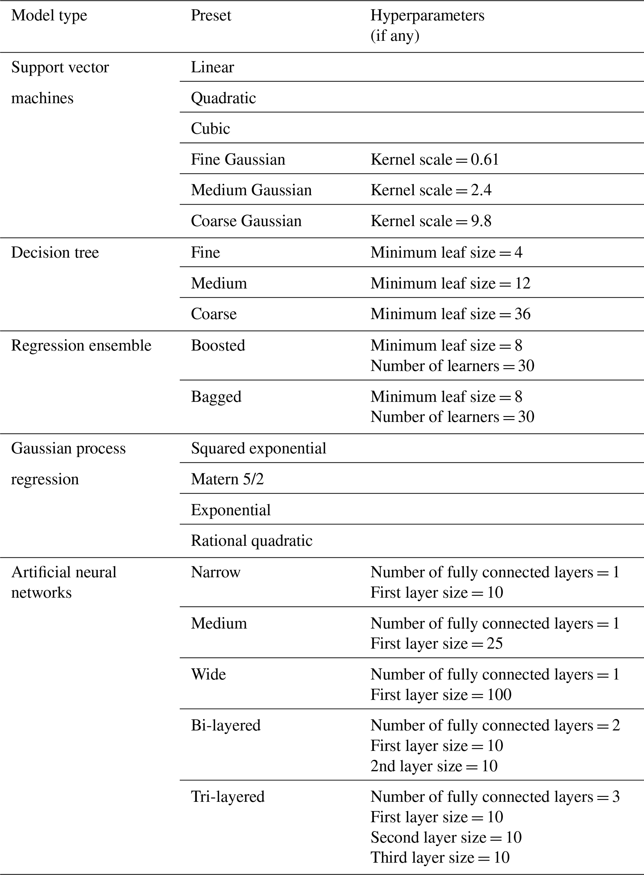
In this study, we present the first high-resolution, long-term daily gridded time series of freshly formed in situ-produced biogenic MSA and nss-SO${}_{\mathrm{4}}^{=}$ (IPB-MSA&SO₄) concentrations over the NA at a 0.25° × 0.25° spatial resolution. The data cover 25 years, from 1998 to 2022, with the possibility of future year-by-year updates. The dataset is a unique and novel product in that it extends the spatial and temporal representativeness of atmospheric in situ observations of marine aerosol chemical properties over the NA by exploiting the potential of machine learning. The dataset represents the sea-level concentrations of MSA and nss-SO${}_{\mathrm{4}}^{=}$, in each grid point of the domain, resulting from the interplay between precursor emissions and local atmospheric conditions. We created the IPB-MSA&SO₄ dataset using in situ MSA and nss-SO${}_{\mathrm{4}}^{=}$ data measured at the Mace Head (MHD) site and during the NAAMES cruises, the gridded dataset from the ECMWF ERA5, and reconstructed F_DMS (Mansour et al., 2023a) as input data. To achieve this aim, we employed the following machine learning (ML) approaches: support vector machines (SVMs), decision tree (DT), regression ensemble (RE), Gaussian process regression (GPR), and artificial neural networks (ANNs). ML has been applied in a variety of scientific areas for model approximation, experiment design, and multivariate regression of oceanic and atmospheric complex systems; however, to our knowledge, no prior applications to MSA and nss-SO${}_{\mathrm{4}}^{=}$ prediction have been published. During model training, we evaluated the various possible kernel functions and hyperparameters in each ML type (details in Table 1), employing the 5-fold cross-validation strategy to select the best-performing (optimal) function capable of properly predicting MSA and nss-SO${}_{\mathrm{4}}^{=}$. A partial dependence analysis is also used to assess the effect of different predictors on the modeled MSA and nss-SO${}_{\mathrm{4}}^{=}$. Furthermore, we investigate the annual and monthly spatial distributions of MSA, nss-SO${}_{\mathrm{4}}^{=}$, and the ratio between them ($\mathrm{MSA}:\mathrm{nss}-{\mathrm{SO}}_{\mathrm{4}}^{=}$) to examine the evolution of MSA and nss-SO${}_{\mathrm{4}}^{=}$ in the different regions of the NA domain from 1998 to 2022. The output data (IPB-MSA&SO₄) from this study should be useful for filling the data gap, particularly for the NA, and be applicable to a variety of investigations, such as climatology, trend analysis, model evaluation, and radiative impact assessment, as well as providing boundary conditions for regional models.

Table 1 List of machine learning models used in the present study.

2 Study domain and data sources

2.1 Study area and measurement sites

The study area extends from 20° to 66° N and from 72° W to the prime meridian (Fig. 1), covering the NA. The key climate-relevant features in the study domain are the Gulf Stream, its northern extension towards Europe known as the North Atlantic Current (NAC), and the cyclonic subpolar gyre (SPG) (Rhein et al., 2011). The Gulf Stream is a warm Atlantic Ocean flow that begins in the Gulf of Mexico and moves through the Straits of Florida before continuing up the eastern coast of the United States (Buckley and Marshall, 2016). These warm northward-flowing waters meet the cold southward-flowing waters of the Labrador Current and the western boundary current of the cyclonic subpolar gyre, ultimately turning east and heading toward northwestern Europe as the NAC. The NAC then splits into multiple branches that enter the subpolar gyre, one of which passes via the Iceland Basin and the other through the Rockall Trough (Fratantoni, 2001). The NA SPG extends from 45 to around 65° N and comprises the sills between Greenland, Iceland, the Faroe Islands, and Scotland. Such circulation phenomena are crucial for the modulation of the temperate climate of northwestern Europe (Marzocchi et al., 2015), and the dynamics of the SPG determine the rate of deep- and intermediate-water formation (sinking dense and cold surface waters through air–sea heat exchanges in the wintertime), particularly in the Labrador Sea (Katsman et al., 2004). Accordingly, they contribute to the regional changes in primary production and the subsequent biogenic emissions in the study domain.

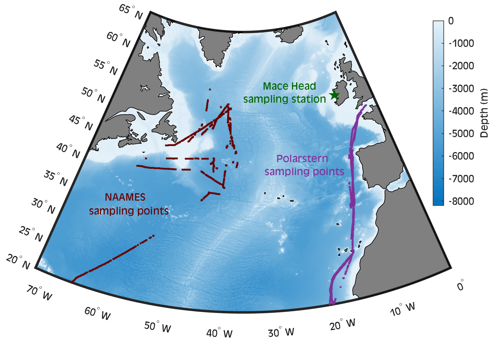
Figure 1 The study region in the North Atlantic (20–66° N, 72–0° W) with bathymetry presented in meters. The gridded bathymetric dataset was extracted from the General Bathymetric Chart of the Oceans (https://www.gebco.net, last access: 25 May 2023) GEBCO_2023 Grid. The green pentagram represents the Mace Head measuring station on the west coast of Ireland, the dark-red points are the sampling points that represent marine conditions in the NAAMES cruises track, and the violet points represent the ship track during Polarstern campaigns.

The MHD Global Atmosphere Watch (GAW) research station (53.33° N, 09.90° W) is located on Ireland's west coast (Fig. 1), about 80 m from the coastline and 21 m above mean sea level. MHD is the only GAW station in the eastern Atlantic region; moreover, it is the globally acknowledged clean background western European station, providing key baseline input for intercomparison with levels elsewhere in Europe (Grigas et al., 2017; O'Dowd et al., 2014).

Four shipboard field campaigns were carried out as part of the NAAMES research project (Behrenfeld et al., 2019). The tracks of cruises representing marine conditions during aerosol sampling (Saliba et al., 2020) are shown in Fig. 1. The measurements cover the periods of November 2015, May–June 2016, September 2017, and March 2018. Behrenfeld et al. (2019) provide a thorough explanation of the NAAMES project's goals, objectives, and atmospheric and oceanic conditions.

2.2 Observational data

Long-term atmospheric concentrations of submicron sulfur aerosol species (methanesulfonic acid, MSA, and sulfate, SO${}_{\mathrm{4}}^{=}$) from January 2009 to June 2018 measured at MHD were used. The measurements were performed using the Aerodyne high-resolution time-of-flight aerosol mass spectrometer (HR-ToF-AMS). The HR-ToF-AMS (DeCarlo et al., 2006) output has a time resolution of ∼ 5–10 min, and the instrument was operated according to the recommendations of Jimenez et al. (2003), Allan et al. (2003), and Canagaratna et al. (2007). MSA was derived from the concentration of the mass fragment CH₃SO${}_{\mathrm{2}}^{+}$ (Ovadnevaite et al., 2014). Further information on the MSA measurement can be found in Mansour et al. (2020a). The black carbon (BC) concentrations were measured in situ at MHD using a multi-angle absorption photometer (O'Dowd et al., 2014) to identify the anthropogenically impacted air masses, as detailed in Sect. 3.1.1.

High-resolution in situ shipborne measurements of non-refractory submicron SO${}_{\mathrm{4}}^{=}$ concentrations were measured every 5 min using HR-ToF-AMS during four open-ocean research cruises (NAAMES) in the northwestern Atlantic: winter (November 2015), late spring (May–June 2016), autumn (September 2017), and early spring (March 2018) (Saliba et al., 2020). We employ this SO${}_{\mathrm{4}}^{=}$ concentration information (no high-resolution MSA datasets available from the NAAMES campaigns) during periods that were largely marine aerosol sources, which were defined as periods when particle number concentrations were <1500 cm⁻³, BC was <50 ng m⁻³, 2 d back trajectories originated from the North Atlantic or tropical Atlantic, and radon concentrations were <500 mBq m⁻³ according to Saliba et al. (2020). The measured SO${}_{\mathrm{4}}^{=}$ from the AMS excludes refractory particles that likely contain the majority of sea-salt sulfate; therefore, the measured SO${}_{\mathrm{4}}^{=}$ is approximately equivalent to nss-SO${}_{\mathrm{4}}^{=}$ (Frossard et al., 2014).

2.3 Air mass back trajectories

The National Oceanic and Atmospheric Administration (NOAA) Air Resources Laboratory (ARL) developed the Hybrid Single-Particle Lagrangian Integrated Trajectory (HYSPLIT4) model (Rolph et al., 2017; Stein et al., 2015), which is used to calculate the air mass back trajectories (BTs). The archived Global Data Assimilation System (GDAS1; 1° × 1°) of the National Centers for Environmental Prediction (NCEP) was used as a driver of the trajectory calculation (ftp://arlftp.arlhq.noaa.gov/pub/archives/gdas1, last access: 10 November 2022). We ran the model at the MHD sampling station as a fixed source location, whereas the NAAMES cruises were run as a moving source location. The starting height was set to 100 m above ground level, and the backward time was 3 d with an interval of 1 h along each entire trajectory track. The schematic diagram of BT calculation is shown in Fig. S1. The arrival frequency of BTs at MHD is 3 h (8 tracks a day), covering the period from 1 January 2009 to 30 June 2018, whereas the arrival frequency of NAAMES is hourly (24 tracks a day), covering the time of the four campaigns identified as marine periods (Saliba et al., 2020).

2.4 Dimethylsulfide flux data

Seawater DMS is the primary contributor to biogenic sulfur aerosol in the atmosphere. For this reason, we use the sea-to-air DMS flux (F_DMS) as a predictor of MSA and nss-SO${}_{\mathrm{4}}^{=}$ concentrations. Mansour et al. (2023a) used an ML predictive algorithm based on Gaussian process regression (GPR) to simulate the distribution of daily seawater DMS concentrations and related F_DMS in the NA areas from 35 to 66° N and from 0 to 55° W at a 0.25° × 0.25° spatial resolution. We extended the GPR model within the NA to encompass the NAAMES measurements, which are essential because they cover the westernmost section of the study area. Figure S2 displays the main differences between the two domains. Simply, the GPR was trained once more, utilizing the same approach as that outlined in Mansour et al. (2023a), with a higher number of data points, and it yielded an enhanced R² value up to 0.77 on the independent test dataset. The daily sea-to-air F_DMS was calculated using the gas transfer velocity (Goddijn-Murphy et al., 2012) and the DMS derived from GPR predictions. For more details about the data product, we refer the reader to Mansour et al. (2023a).

2.5 Meteorological data

The ECMWF ERA5 reanalysis data (Hersbach et al., 2020) were downloaded to extract the meteorological parameters used as predictors of MSA and nss-SO${}_{\mathrm{4}}^{=}$ in the ML models. ERA5 provides estimates for the hourly state of the atmosphere, worldwide, with a 0.25° × 0.25° spatial resolution at the surface and different pressure levels. From the global domain, we extracted multiple atmospheric components, including air temperature at 2 m above sea level (AT) and surface net shortwave radiation flux (SRF), as representative of thermal heating, and the relative humidity (RH), as representative of water vapor abundance in the atmosphere. To represent the dispersion of aerosol particles in the troposphere and wet removal through the below-cloud scavenging process, the boundary layer height (BLH) and the precipitation rate (PR) were utilized, respectively.

3 Methods

3.1 Data preparation

In this section, we describe the preparation of predictors and responses that were used to train, cross-validate, and generate the ML models.

3.1.1 Air mass selection

In previous studies (Mansour et al., 2020b; O'Dowd et al., 2015; Ovadnevaite et al., 2014), the BC concentration has often been considered to be a useful tool to select clean marine air masses excluding inputs from continental emissions or ship trails. In this study, we still relied on BC measurements as a precious tool to identify and exclude anthropogenically impacted air masses, but we also developed a more complete approach aimed at identifying air masses characterized by a high degree of contact with the ocean surface. This was necessary in order to select, from the in situ observations, data points representing almost entirely oceanic sources to provide the best dataset for training the ML models.

The retention ratio of the air mass over the ocean (R_O) was calculated to determine whether an air mass (identified by BT track) arriving at the MHD sampling station or at the ship location, in the case of shipborne measurements, was primarily from the NA region or not. We used 3 d BTs arriving 100 m above the MHD sampling station and NAAMES tracks. The BT tracks at the MHD arrival point were calculated 8 times per day, whereas they were calculated 24 times per day at NAAMES measuring points, considering only the measurements classified as marine periods (Saliba et al., 2020). The R_O was calculated for each track as follows:

$$\begin{array}{}\text{(1)}& R_{\mathrm{O}}={\displaystyle \frac{{\sum }_{i=\mathrm{1}}^{N_{\mathrm{Ocean}}}{e}^{\frac{-t_i}{\mathrm{72}}}}{{\sum }_{i=\mathrm{1}}^{N_{\mathrm{Total}}}{e}^{\frac{-t_i}{\mathrm{72}}}}},\end{array}$$

where N_Total is the total number of trajectory endpoints, which is equal to 73 (arrival point + 72 backward hours); N_Ocean is the total number of trajectory endpoints passing over the ocean; and t_i is the backward-tracking time, with the unit of hours and spanning values from 0 to 72. Because air mass diffusion and particle deposition potentially occur during the air mass transport, a weighting factor $e^{-t_i/\mathrm{72}}$ related to tracking time has been introduced. The weighting factor takes values from 1 (at the arrival point) up to 0.37 (farthest point); hence, oceanic areas far from the arrival point, corresponding to longer backward-tracking time, have a weaker influence than areas closer to the sampling point. As a result, a higher R_O value implies that oceanic emissions have a greater influence on the air mass and that the source region is more likely to be the ocean. Other studies have used similar methods to characterize air mass source regions. For example, Zhou et al. (2021) studied the contribution of nonmarine MSA sources in the coastal East China Sea and the Gulf of Aqaba by characterizing the land air masses. Rinaldi et al. (2021) used a combination of low-traveling air mass BTs and satellite ground-type maps to investigate the effect of ground conditions (sea ice, snow, seawater, and land) on air samples at Ny-Ålesund station in the Arctic Ocean.

Because oceanic air masses crossing the NA can pass above the BLH, its connection to local sea surface processes, such as marine biogenic emission and subsequent atmospheric reactions, may be significantly weaker. To address this issue, Eq. (2) was used to calculate the retention ratio of an ocean air mass within the marine boundary layer (R_B).

$$\begin{array}{}\text{(2)}& R_{\mathrm{B}}={\displaystyle \frac{{\sum }_{i=\mathrm{1}}^{N_{\mathrm{Below}}}{e}^{\frac{-t_i}{\mathrm{72}}}}{{\sum }_{i=\mathrm{1}}^{N_{\mathrm{Ocean}}}{e}^{\frac{-t_i}{\mathrm{72}}}}},\end{array}$$

where N_Ocean is the total number of trajectory endpoints located over the ocean (i.e., marine endpoints) and N_Below is the number of marine endpoints with an altitude below the BLH. The higher the R_B value, the more airflow over the ocean is confined to the MBL. The BLH datasets at each endpoint were extracted from the hourly ERA5 dataset.

The total number of BT tracks arriving at MHD during the period from January 2009 to June 2018 is 27 744 (3468 d × 8 tracks per day). We counted the number of endpoints of all BTs in each 1° × 1° grid cell and normalized them to the maximum value to find the percentage of endpoints for all grid cells (Fig. S3). The larger density of BT endpoints is concentrated over the NA oceanic region, indicating that the main source regions for air masses transported to MHD sampling stations are most likely oceanic. At MHD, we investigated how MSA (a marine biogenic tracer) responds to change in BC (a tracer of anthropogenic input), as seen in Fig. S4, by considering hourly data simultaneous to the arrival time of BTs (i.e., 8 times a day). We found that MSA tends to fluctuate minimally when BC is less than 15 ng m⁻³ (slope = 0.05), whereas MSA tends to rise slightly when BC exceeds 15 ng m⁻³ (slope = 0.28). Such cases with hourly BC concentrations <15 ng m⁻³ were classified as representative of marine conditions, which are likely not influenced by anthropogenic sources. To constrain the impact of marine biogenic emissions and meteorological parameters on MSA and nss-SO${}_{\mathrm{4}}^{=}$, air masses were included in this analysis only if they were characterized by $R_{\mathrm{O}}+R_{\mathrm{B}}\ge \mathrm{1.75}$, meaning that the air mass had experienced a high degree of contact with the ocean surface within the last 3 d (Fig. S4). Indeed, considering the above condition, an air mass must have an R_O equal to at least 0.75 and, in such case, the track must be traveling below the BLH 100 % of the time. By introducing the criterion of $R_{\mathrm{O}}+R_{\mathrm{B}}\ge \mathrm{1.75}$, approximately 72 % of the BT tracks were considered. This reflects the significance of the MHD research station for studying NA biogenic emissions as well as the frequency with which it is impacted by MBL air masses (Grigas et al., 2017; O'Dowd et al., 2014). After considering the BC threshold (<15 ng m⁻³) and conservatively removing all of the observations done when the BC data were unavailable (instrument downtime), 9211 (33 % of the total) tracks were classified as representative of marine conditions (selected marine BTs frequency is presented in Fig. S5).

Regarding the NAAMES measurements, the total number of calculated BT tracks was 832 (Fig. S6) during background marine conditions, identified by Saliba et al. (2020). In this study, we kept 660 tracks (Fig. S7) of the above 832 as representative samples of marine conditions during NAAMES cruises by limiting the analysis to hourly samples with $R_{\mathrm{O}}+R_{\mathrm{B}}\ge \mathrm{1.75}$.

3.1.2 Predictor extraction along back trajectories

In order to train the ML models, it was necessary to associate each observed MSA and nss-SO${}_{\mathrm{4}}^{=}$ data point with the corresponding potential predictors. The potential predictors (F_DMS, AT, SRF, RH, BLH, and PR) were extracted at each endpoint of the BTs associated with each of the selected clean marine observational data points (see Sect. 3.1.1), inside the oceanic region within 20–66° N and 0–72° W (Fig. S1). The extracted predictor values were then averaged along each marine BT track, providing the most representative picture of the conditions (air mass history) that led to the formation of the observed sulfur aerosol concentrations. The few endpoints over land or crossing above the BLH were eliminated.

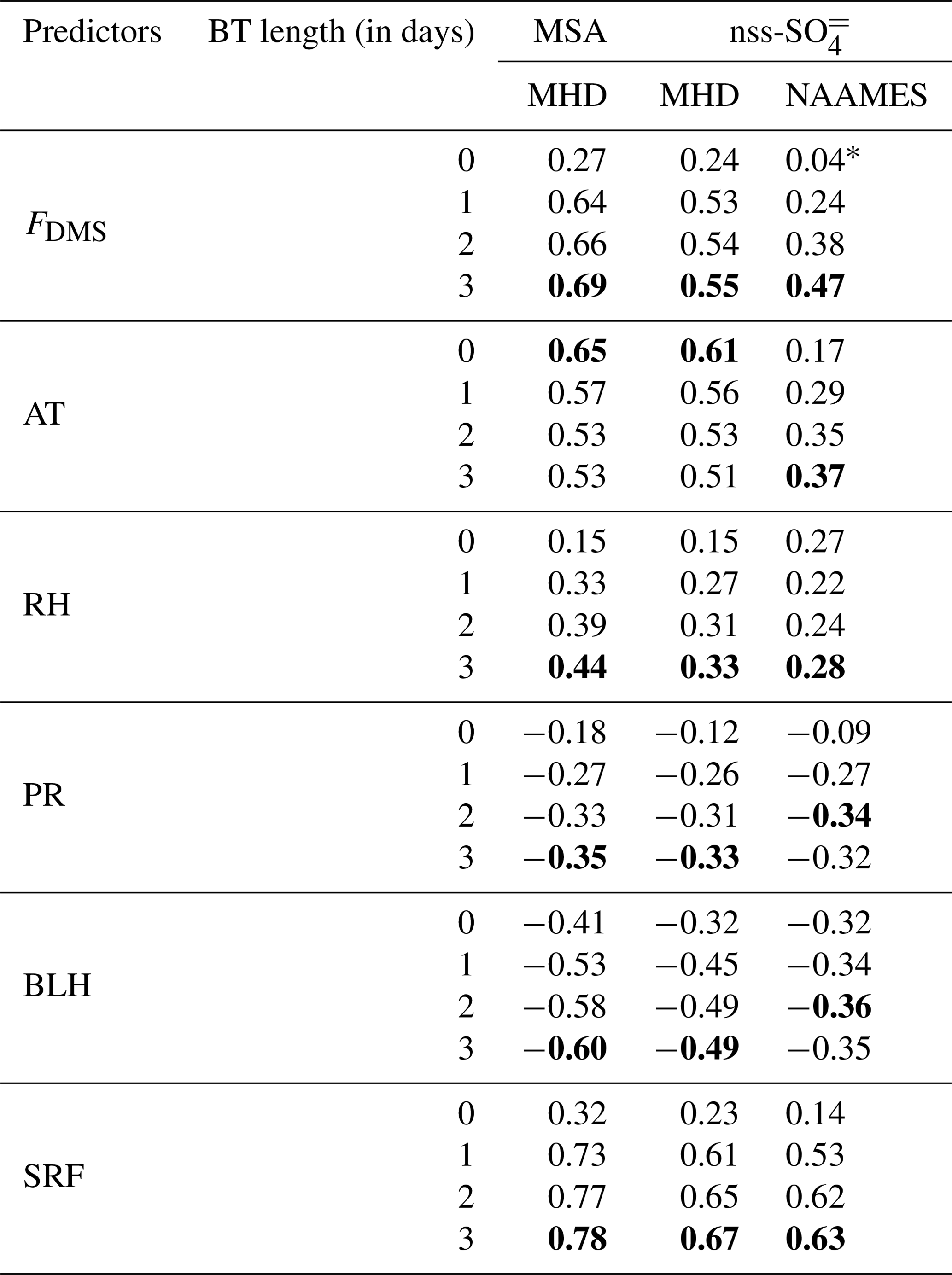
The Pearson correlation coefficients between the potential predictors and observational MSA and nss-SO${}_{\mathrm{4}}^{=}$ data were compared, considering different BT lengths of 1, 2, and 3 d, to assess which BT length was more representative of the timescale of sulfur aerosol formation processes. As seen from Table 2, both MSA and nss-SO${}_{\mathrm{4}}^{=}$ correlate better with F_DMS considering a 3 d BT length. Similarly, the majority of the other predictors, except for AT, tended to maximize their correlations considering a 2 or 3 d BT length. Ultimately, for each predictor, we considered the BT length that maximized the correlation coefficient for the analyses in the present study.

Table 2 The Pearson coefficients between possible predictors for the selected marine air masses and the in situ observed MSA and nss-SO${}_{\mathrm{4}}^{=}$ concentrations. The MSA, nss-SO${}_{\mathrm{4}}^{=}$, and F_DMS values are used on a log scale. All values are statistically significant at p<0.05, except the value indicated by “*”. Bold text denotes the maximum during different days of air mass history.

3.1.3 Responses at measuring sites

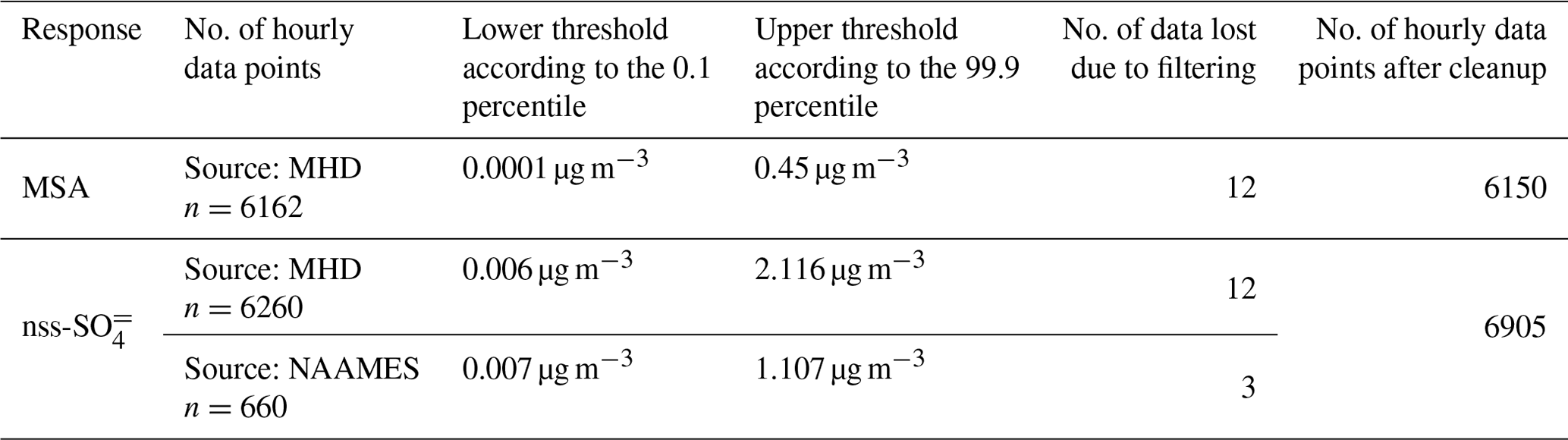
Hourly nss-SO${}_{\mathrm{4}}^{=}$ at MHD and from the NAAMES campaigns as well as MSA at MHD, measured concurrently with the selected marine BTs (Sect. 3.3.1), were used to build ML models. A total of 6162 (6920) data points for MSA (nss-SO${}_{\mathrm{4}}^{=}$) were obtained. Furthermore, we also applied a 0.1 and 99.9 percentile lower and upper threshold filter to remove the extremely low and high values that could bias the ML models' training and cross-validation. This helped to identify and remove outliers in each dataset, thereby reducing the number of data points to 6150 (6905) for MSA (nss-SO${}_{\mathrm{4}}^{=}$) (∼0.2 % of data points were rejected). Details of the MSA and nss-SO${}_{\mathrm{4}}^{=}$ percentile thresholds, along with the number of data before and after applying the filters are given in Table 3. The hourly data after cleanup are used for training/cross-validation and testing of ML models.

Table 3 Details of the number of hourly (MSA and nss-SO${}_{\mathrm{4}}^{=}$) data points corresponding to selected marine BTs. The threshold used for filtering outlier values and the number of data points after filtering are given.

3.2 Machine learning models

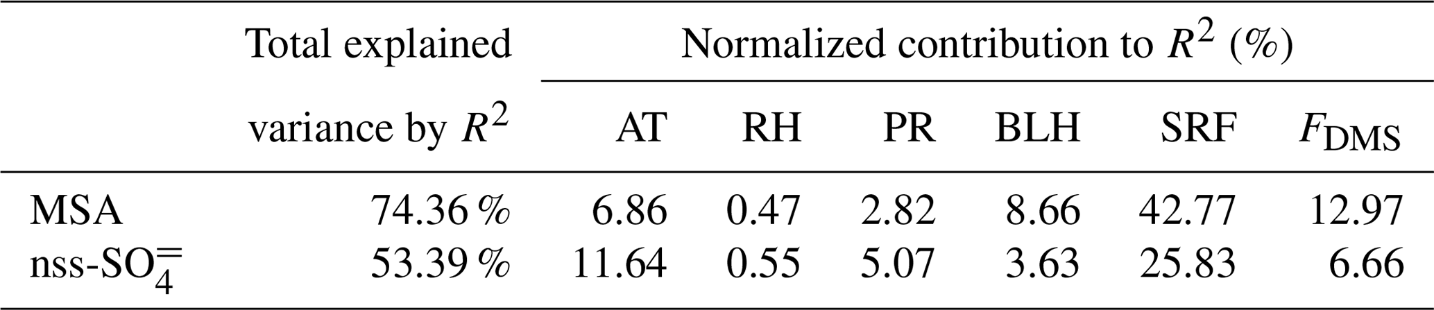
The methodological flowchart of the present study is shown in Fig. 2. The core of the framework uses supervised ML regression techniques to build predictive models for estimating the atmospheric concentrations of biogenic MSA and nss-SO${}_{\mathrm{4}}^{=}$ (responses) from independent variables (predictors). Predictors include the sea-to-air F_DMS and meteorological parameters that control the aerosol concentration in the MBL. We used multilinear regression to assess the contribution of each predictor to MSA and nss-SO${}_{\mathrm{4}}^{=}$ variations. Initially, we ran the multilinear regression model using the total of the following potential six predictors: F_DMS, AT, SRF, RH, BLH, and PR. Secondly, we applied the multilinear regression models by eliminating one predictor each time. Each independent variable's contribution to R² is the reduction in total R² when that variable is eliminated. The results (Table 4) showed that the six predictors used can explain up to 74 % (53 %) of MSA (nss-SO${}_{\mathrm{4}}^{=}$) variance. Such predictors tend to contribute differently to MSA and nss-SO${}_{\mathrm{4}}^{=}$. SRF, F_DMS, and the BLH are the most effective parameters for MSA (explaining up to 64 % of the variability), while SRF, AT, and F_DMS are the most influential with respect to nss-SO${}_{\mathrm{4}}^{=}$ (explaining up to 44 % of the variability). RH has a minor contribution to the MSA and nss-SO${}_{\mathrm{4}}^{=}$ variance. To know if a predictor contributes significantly to the explained variance, we performed an analysis of variance (ANOVA) on the implemented multilinear regression model. The ANOVA revealed that all of the tested predictors have statistically significant (p<0.05) contributions to MSA and nss-SO${}_{\mathrm{4}}^{=}$. For these reasons, we applied the ML models using all six potential predictors.

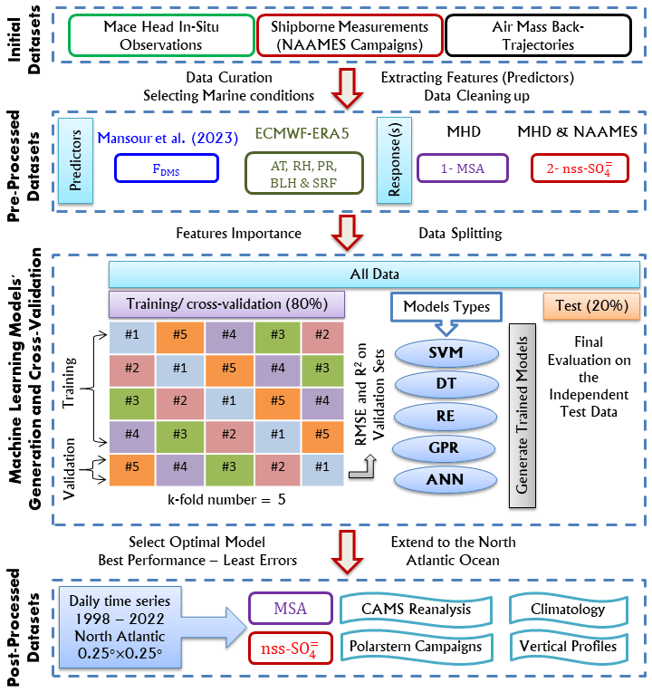
Figure 2 The methodology's workflow, showing the predictor and response variable data preparation, the overall framework for the generation and development of the trained models (including a schematic diagram of 5-fold cross-validation, model export and validation details), and post-processing analysis.

Table 4 Multilinear regression of MSA and nss-SO${}_{\mathrm{4}}^{=}$ as a function of predictors. The MSA, nss-SO${}_{\mathrm{4}}^{=}$, and F_DMS values are used on a log scale. Each independent variable's contribution to R² is the decrease in total R² when that variable is eliminated. Individual R² contributions are normalized and added together to equal the overall R². According to the analysis of variance (ANOVA) on the multilinear regression models, all predictors have a statistically significant (p<0.05) contribution to the MSA and nss-SO${}_{\mathrm{4}}^{=}$ variance.

The datasets, containing the corresponding predictors and each one of the responses (MSA and nss-SO${}_{\mathrm{4}}^{=}$) separately, were split randomly into two subsets, defined as the training/cross-validation set and the test/evaluation set, for each response. The training/cross-validation sets include 80 % of the total points (n=4920 for MSA and n=5524 for nss-SO${}_{\mathrm{4}}^{=}$), while the test/evaluation sets comprise the remaining 20 % (n=1230 for MSA and n=1381 for nss-SO${}_{\mathrm{4}}^{=}$). To improve ML algorithms' accuracy and protect against overfitting, a k-fold cross-validation strategy with k=5 was used, as this has been shown to provide maximal model prediction robustness and minimal bias (Rodriguez et al., 2010; Fushiki, 2011). The k-fold cross-validation is a procedure used to estimate the skill of the model on new data and generally results in a less biased estimate of the model skill. The k-fold number refers to how many groups a given data sample is to be split into. In this study, where k=5, the training/cross-validation dataset was further randomly divided into five folds of roughly equal size. For each trial, one group is designated as a holdout or validation dataset, while the remaining four groups are designated as training data (Fig. 2). The model is then fit on the training set (four folds) and evaluated on the validation set (last fold), and the average evaluation measures (accuracy) on the validation subsets of the five iterations are reported. To better examine the model's repeatability on a new independent dataset, the generated models were evaluated on the test data that were not included in the model construction.

Five types of ML models were trained/cross-validated and evaluated to identify the best-performing model with respect to estimating sulfur aerosol concentrations (MSA and nss-SO${}_{\mathrm{4}}^{=}$). The ML algorithms are SVM, DT, RE, GPR, and ANN. These are the most common types of algorithms; however, there are subtypes for which advanced options and optimizations in the model can increase the performance and resilience of the algorithms. In general, each supervised ML model performs differently and has various strengths and shortcomings. Finding the proper ML algorithm is largely based on trial and error; even experienced data scientists cannot anticipate if an algorithm will work without testing it. Thus, understanding the fundamentals of various ML algorithms and their applicability to diverse applications is critical (Sarker et al., 2019). As a result, we initially assessed 20 algorithms belonging to the aforementioned five types and chose the model with the best performance skill from each type (Table 1), as detailed in the following sections.

3.2.1 Support vector machines (SVMs)

A SVM is a powerful mathematical model based on the statistical learning theory (Vapnik, 2013) that can be used either for classification or regression analysis. In recent decades, SVMs have demonstrated high prediction accuracy for a wide range of regression problems in fields such as oceanography, meteorology, and atmospheric sciences (Lins et al., 2013; Sachindra et al., 2018; Shabani et al., 2020; Shrestha and Shukla, 2015; Fan et al., 2018). The SVM model estimates the regression using a series of kernel functions that are capable of implicitly converting the original, lower-dimensional input data to a higher-dimensional feature space. To achieve the best prediction accuracy for MSA and nss-SO${}_{\mathrm{4}}^{=}$, we assessed the different SVM kernel functions, such as linear, polynomial (quadratic and cubic), and Gaussian (Table 1). The Gaussian kernel was adopted by trying various kernel scales, setting them to 0.61 (fine), 2.4 (medium), and 9.8 (coarse). For more information on SVMs, the reader is referred to https://www.mathworks.com/help/stats/fitrsvm.html (last access: 10 January 2023).

3.2.2 Decision tree (DT)

The DT model is a nonparametric, nonlinear model that generates a structure resembling a tree for classification and regression (Kotsiantis, 2013; Quinlan, 1986). It repeatedly divides the dataset into smaller subsets based on independent features from the input dataset. The split seeks to reduce variability within each group while increasing the variance between subsets. The final tree is made up of decision and leaf nodes. The decision node represents a condition on an attribute, and its branches indicate the conditions' outcomes. For additional information on DT, the reader is directed to https://www.mathworks.com/help/stats/fitrtree.html (last access: 10 January 2023). The critical parameter in this technique is determining when to terminate the division process. In this study, we set up three different minimum leaf sizes (minimum samples to split) to control the number of data that should be in the sub-branch to continue the splitting process, namely 4 (fine tree), 12 (medium tree), and 36 (coarse tree), as seen in Table 1.

3.2.3 Regression ensemble (RE)

RE is a technique that employs a collection of DT models (referred to as weak learners or base models), each of which is produced by applying a learning process to a specific problem and then combining them to provide the final prediction (Mendes-Moreira et al., 2012). The performance and accuracy of ensembles are determined by the aggregation of weak learners (Hengl et al., 2018). The well-known types of aggregation are the bagging and boosting methods (Breiman, 2001). In the bagging method (also known as bootstrap aggregating), the base models are generated using random subsamples drawn from the original dataset with the bootstrap sampling method, where some original examples appear several times, whereas others do not appear at all. On the other hand, the main idea of the boosting method is that it is possible to convert a base model that performs slightly better into one that arbitrarily achieves high accuracy. This conversion is performed by combining the estimations of several predictors. For more information on RE, the reader is referred to https://www.mathworks.com/help/stats/fitrensemble.html (last access: 10 January 2023).

3.2.4 Gaussian process regression (GPR)

GPR is a nonparametric technique for solving nonlinear regression problems (Williams and Rasmussen, 1996) that is based on Bayesian theory and statistical learning theory. The accuracy of GPR is dependent on the adopted kernel (covariance) functions (Verrelst et al., 2016). We assessed the different base kernel functions, namely exponential, Matern 5/2, squared exponential, and rational quadratic (Asante-Okyere et al., 2018; Mansour et al., 2023a) to determine the optimal covariance function that could produce reliable predictions of MSA and nss-SO${}_{\mathrm{4}}^{=}$. For more information on GPR, the reader is referred to Mansour et al. (2023a) and https://www.mathworks.com/help/stats/fitrgp.html (last access: 10 January 2023).

3.2.5 Artificial neural networks (ANNs)

An ANN is an information processing system that can be used to understand the complex nonlinear relationship between the response and predictors (Kalogirou, 2001). It consists of interconnected groups of artificial neurons that work in the same way as biological neurons. The ANN structure comprises three distinctive groups called input (corresponds to the predictors), several hidden layers (fully connected), and output (corresponds to the predicted response values). The input introduces data to the ANN model, the hidden layer processes the data, and the results are produced in the output. Further details on ANNs can be found at https://www.mathworks.com/help/stats/fitrnet.html (last access: 10 January 2023). We trained various types of ANNs as single-layer (number of fully connected layers = 1), bi-layered (number of fully connected layers = 2), and tri-layered (number of fully connected layers = 3) neural networks, as detailed in Table 1.

3.3 Evaluation measures

In this study, we use different validation metrics to evaluate the ML models' performance. Each of the metrics is calculated using “residuals”. Residuals are the differences between the observed data points O_i and the predicted values P_i, where $i=\mathrm{1},\mathrm{2},\mathrm{\dots }n$; here, n refers to the number of observations. Better models with respect to predicting the response have residuals close to zero. The average magnitude of the residuals is called mean absolute error (MAE):

$$\begin{array}{}\text{(3)}& \mathrm{MAE}={\displaystyle \frac{\mathrm{1}}{n}}{\sum }_{i=\mathrm{1}}^n\left|O_i-P_i\right|.\end{array}$$

Regression models tend to use the square of the residuals instead of the absolute. The square root of the average of the squared residuals is called the root-mean-square error (RMSE). A low RMSE denotes confidence that the model has relatively few large errors.

$$\begin{array}{}\text{(4)}& \mathrm{RMSE}=\sqrt{{\displaystyle \frac{\mathrm{1}}{n}}{\sum }_i^n(P_i-O_i{)}^{\mathrm{2}}}\end{array}$$

The metrics listed in Eqs. (3) and (4) can only provide information on how a model compares to observations and/or other models. Neither can objectively say whether a model is a good fit for the data. Comparing a model to a simple baseline model is a different approach. This is the motivation behind the use of the coefficient of determination (R²) metric (Eq. 5). R² is the relative difference in the total error obtained by fitting a model, resulting in a value of between 0 and 1. If a model fits the data well, the model error is small and R² will be close to 1, and vice versa.

$$\begin{array}{}\text{(5)}& R^{\mathrm{2}}=\mathrm{1}-{\displaystyle \frac{{\sum }_i^n(O_i-P_i{)}^{\mathrm{2}}}{{\sum }_i^n(O_i-\stackrel{\mathrm{‾}}{O_i}{)}^{\mathrm{2}}}},\end{array}$$

where $\stackrel{\mathrm{‾}}{O_i}$ is the average of observations. The predicted–observed linear slope is the last metric used to evaluate the performance of ML models. It determines the rate of change in the predicted variable concerning the observed variable and should be close to unity for skilled model predictions.

4 Results and discussion

4.1 Evaluation of ML model performance

As a first step, we assessed different possible hyperparameter optimizations in each of the five types of ML models used (SVM, DT, RE, GPR, and ANN) to determine which one had the best fit and lower errors for sulfur aerosol (MSA and nss-SO${}_{\mathrm{4}}^{=}$) predictability. We chose the best model with the lowest errors in each type for further evaluation and analysis based on the evaluation measures (RMSE, MAE, and R²). The evaluation measures are summarized in Table S1. The medium Gaussian SVM, which utilizes a Gaussian kernel scale equal to the square root of the number of predictors (2.4), displayed better performance. The coarse DT, which sets the minimum sample size to split equal to 36; the ensemble bagged trees (EBT) of a bootstrap aggregated ensemble; and the GPR, which employs the rational quadratic kernel, represent the minimum errors. Finally, a medium ANN of layer size 25 with one fully connected layer was selected. The five best-performing (optimal) models were exported and saved so that they could be used to make new predictions on a new dataset.

Figures 3a–e and 4a–e present a detailed comparison between observed and predicted MSA and nss-SO${}_{\mathrm{4}}^{=}$, respectively, for the five optimal ML models developed. When compared with the multilinear regression (Table 4), it is clear that ML models can generally reconstruct the observations with a markedly higher R² value, which means that the selected ML approaches capture much more of the observed MSA and nss-SO${}_{\mathrm{4}}^{=}$ variability. While the five applied optimal algorithms have quasi-similar measures, the best model for predicting MSA and nss-SO${}_{\mathrm{4}}^{=}$ is GPR. For hourly MSA (nss-SO${}_{\mathrm{4}}^{=}$), GPR achieves the highest R² value of 0.79 (0.64) and the lowest RMSE of 0.362 (0.282) for the cross-validated data (average measures of each validation fold). When extending this to the test data, the R² and RMSE reach 0.81 (0.67) and 0.347 (0.272), respectively. The EBT comes second in terms of performance with respect to predicting MSA (nss-SO${}_{\mathrm{4}}^{=}$) with an R² of 0.80 (0.64) for the independent test data. The SVM and ANN achieve a reasonable accuracy with a respective R² value of 0.79 (0.61) and 0.78 (0.60) for MSA (nss-SO${}_{\mathrm{4}}^{=}$) based on the test data. Lastly, based on the hourly test data, DT shows the lowest, although still respectable, accuracy with an R² of 0.76 for MSA and of 0.57 for nss-SO${}_{\mathrm{4}}^{=}$.

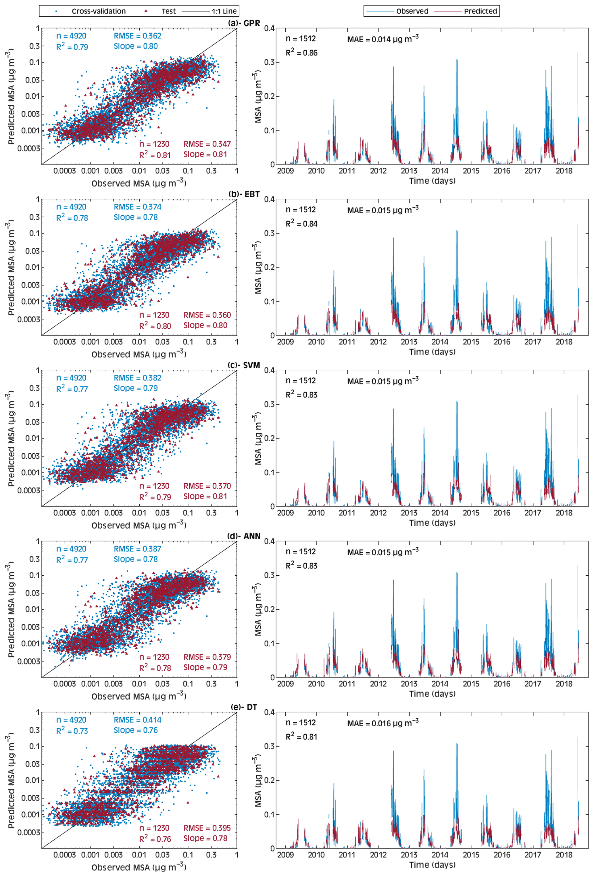
Figure 3 Comparison of predicted and observed MSA on the hourly (left panels) and daily (right panels) scales: (a) GPR, (b) EBT, (c) SVM, (d) ANN, and (e) DT. The validation and test data subsets are used to compute the model's performance. R² and RMSE are computed in a logarithmic space, whereas MAE is computed on a normal scale.

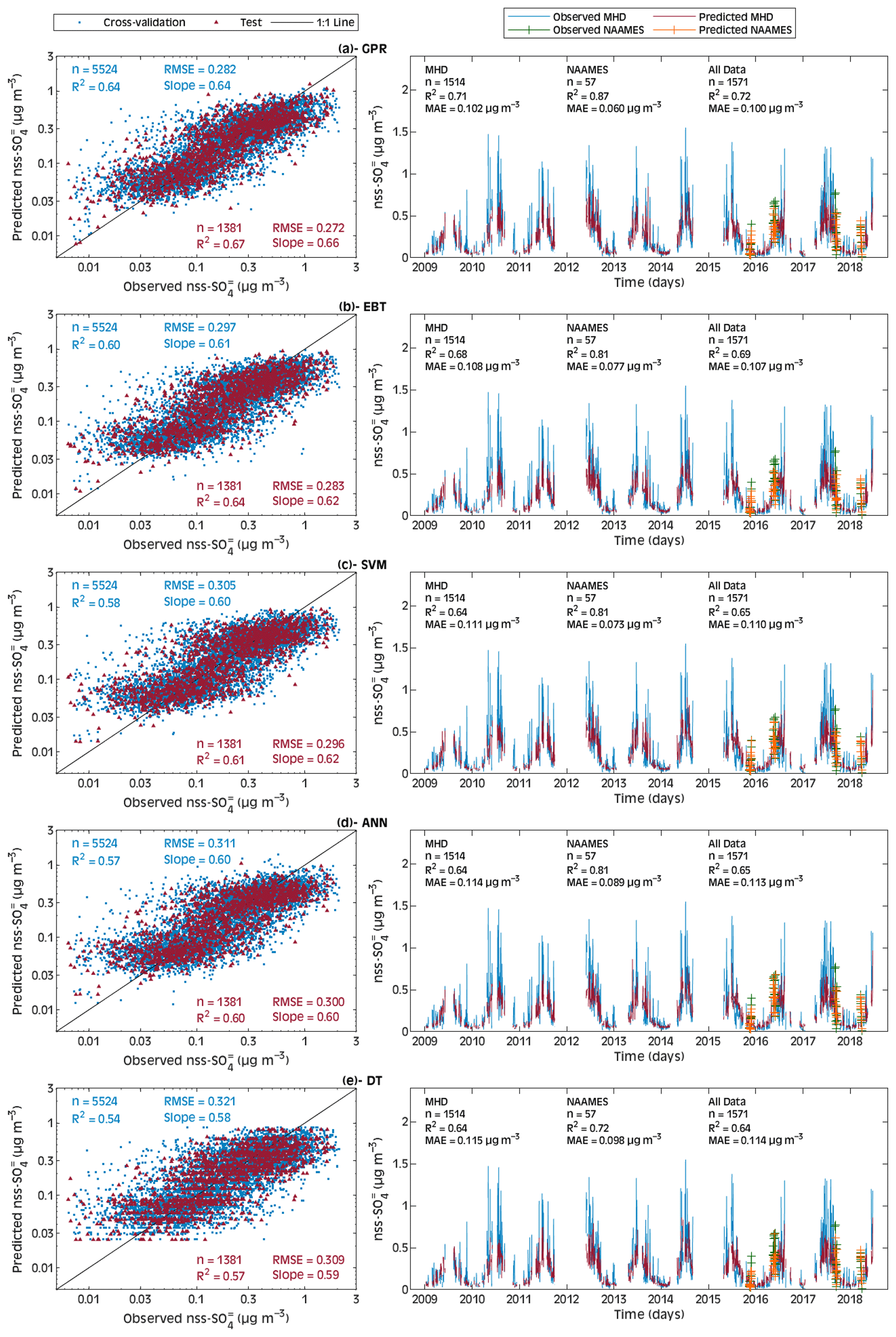
Figure 4 Comparison of predicted and observed nss-SO${}_{\mathrm{4}}^{=}$ on the hourly (left panels) and daily (right panels) scales: (a) GPR, (b) EBT, (c) SVM, (d) ANN, and (e) DT. The validation and test data subsets are used to compute the model's performance. R² and RMSE are computed in a logarithmic space, whereas MAE is computed on a normal scale.

Importantly, the implemented ML models can reconstruct MSA and nss-SO${}_{\mathrm{4}}^{=}$ daily time series' characteristics with remarkable consistency between observed and predicted data, except for extremely high and low concentrations. This is mostly due to the low probability of such concentrations in the observed dataset, which inhibits ML models from reconstructing them. The quantitative comprehension of exceptional emission extremes is not addressed in this study; nonetheless, their occurrence and possible implications deserve to be investigated in future studies. It is worth noting that the daily averages of MSA and nss-SO${}_{\mathrm{4}}^{=}$ have been calculated from the validation folds and the test set. The MAE of GPR is close to 0.014 (0.100) µg m⁻³ for MSA (nss-SO${}_{\mathrm{4}}^{=}$). The MAE values of EBT, SVM, ANN, and DT are higher than those of GPR. According to the R², the ranking order is the same as for the MAE, i.e., GPR outperforms EBT, SVM, ANN, and DT for both MSA and nss-SO${}_{\mathrm{4}}^{=}$, although the differences in the R² values of the five models are small. An in-depth look at the MAE and R² from MHD and NAAMES (Fig. 4, right panels) demonstrates that the ML models perform well with respect to predicting nss-SO${}_{\mathrm{4}}^{=}$ across different datasets. All five models show relatively high R² values for the NAAMES dataset. EBT, SVM, and ANN have R² values that are similar (equal to 0.81), whilst GPR has the highest R² value (reaching 0.87) and DT has the lowest (0.72). In essence, the performance metrics indicate that GPR always has the highest accuracy and lowest errors, reflecting the robustness of GPR. Therefore, GPR was selected as the optimal regressor for further analysis in this study.

Knowing that the GPR model could be biased due to the inhomogeneous distribution of in situ observations, we assessed the applicability of the GPR model in regions poorly covered by atmospheric observational data (such as the central part of the domain) by running the model in a worst-case scenario deployment. In this exercise, we predicted the daily variations in nss-SO${}_{\mathrm{4}}^{=}$ measurements in the westernmost portion of the study area by training the model using only observations from the eastern part of the domain (i.e., data collected at MHD). In this case, MHD data were used for training/cross-validation, while the four NAAMES campaigns were employed as independent test data. The evaluation on the test data (Fig. S8) revealed that GPR can explain 55 % of the daily observed nss-SO${}_{\mathrm{4}}^{=}$ variance (MAE = 0.129 µg m⁻³), even in this worst-case scenario and on a limited test dataset (n=57). This more-than-acceptable model performance supports the reliability of the IPB-MSA&SO₄ dataset in the central part of the NA, where measurements of MSA and nss-SO${}_{\mathrm{4}}^{=}$ are missing. In addition, Sect. 4.5 describes the validation of the GPR model with respect to predicting observed MSA concentrations during the Polarstern campaigns, which were not included in either the model training/cross-validation or in the model test.

4.2 Partial dependence analysis

Most ML models are referred to as “black box” models, as the internal computations inside multiple operational layers in a model are concealed, and most systems have only observable inputs and outputs out of the box. A partial dependence analysis (Friedman, 2001) is used to assess how predictors influence ML model output and shows whether the relationship between the response and any of the features is linear, monotonic, or more complex. The method entails altering one feature and constraining the remaining features to unaltered average values to illustrate the marginal effect of the changed feature on the expected outcome. The partial dependence plots of MSA and nss-SO${}_{\mathrm{4}}^{=}$ as a function of the predictors in the best-performing GPR model are shown in Fig. 5; these plots indicate that the interactions between predictors and response are generally complex. MSA and nss-SO${}_{\mathrm{4}}^{=}$ levels tend to rise as F_DMS levels rise from 3 to 10 µmol m⁻² d⁻¹. MSA continues to rise with stronger F_DMS emission rates (>10 µmol m⁻² d⁻¹); nevertheless, the nss-SO${}_{\mathrm{4}}^{=}$ concentration appears independent of F_DMS after this threshold. AT exhibits a positive relationship with MSA and the nss-SO${}_{\mathrm{4}}^{=}$ concentration in the range of 5–15 °C and a negative relationship above 15 °C. RH, which has the least impact on MSA and nss-SO${}_{\mathrm{4}}^{=}$ (Table 4), has an unclear pattern regarding the MSA and nss-SO${}_{\mathrm{4}}^{=}$ marginal changes. MSA and nss-SO${}_{\mathrm{4}}^{=}$ present a negative dependence on PR, as rain is expected to scavenge aerosol particles; nevertheless, at higher PR levels, nss-SO${}_{\mathrm{4}}^{=}$ concentrations tend to increase. This may be partly linked to enhanced cloudiness, associated with high PR, where the aqueous-phase formation of nss-SO${}_{\mathrm{4}}^{=}$ in the MBL may be favored (Zhu et al., 2006; von Glasow and Crutzen, 2004). This is also in agreement with the enhancement of the nss-SO${}_{\mathrm{4}}^{=}$ concentration at high RH. Finally, BLH and SRF are the parameters that show the most straightforward influence on the MSA and nss-SO${}_{\mathrm{4}}^{=}$ levels, with a deep BLH resulting in a dilution of their concentrations and high SRF leading to high MSA and nss-SO${}_{\mathrm{4}}^{=}$ levels, as expected for DMS photooxidation products.

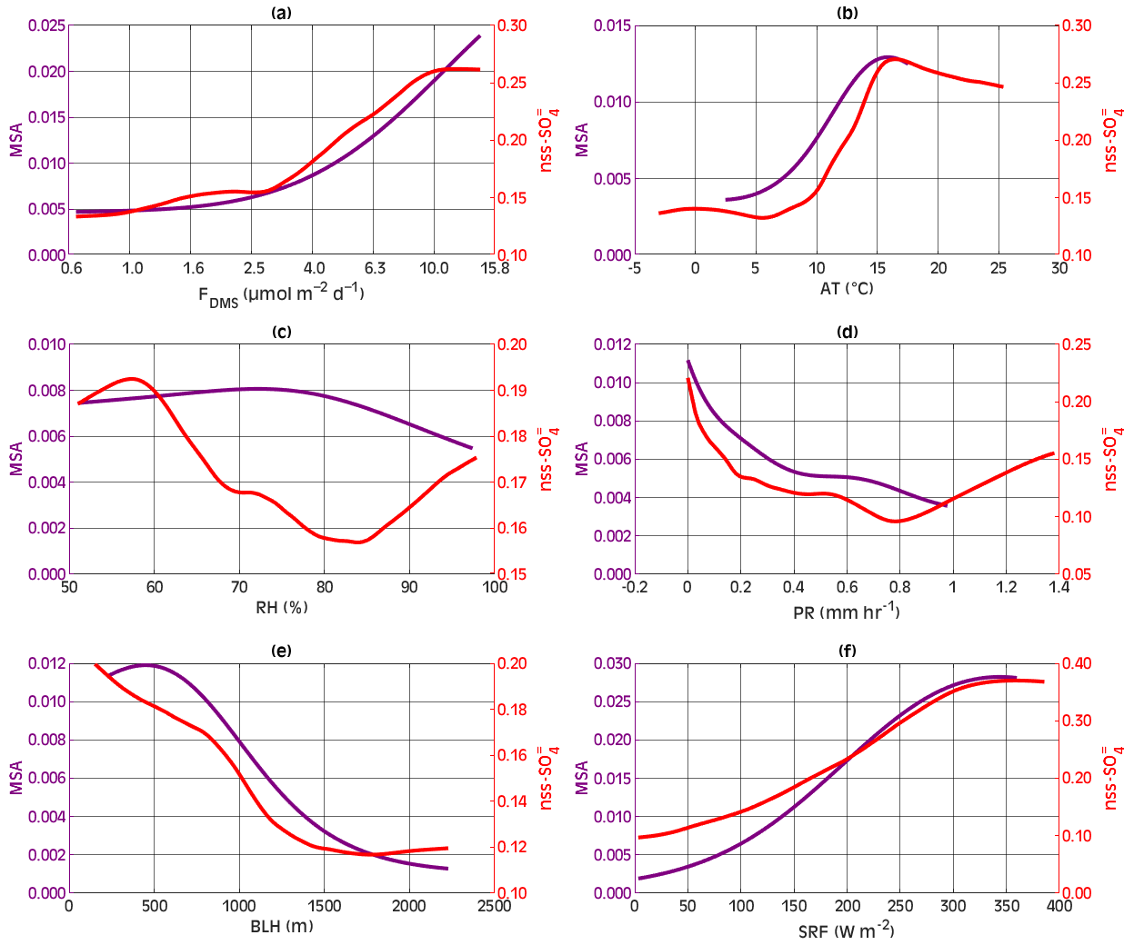
Figure 5 Partial dependence plots of MSA and nss-SO${}_{\mathrm{4}}^{=}$ as a function of the predictors revealed by the GPR model.

4.3 The IPB-MSA&SO₄ dataset

The GPR model was used to generate the long-term gridded fields of high-resolution (0.25° × 0.25°) MSA and nss-SO${}_{\mathrm{4}}^{=}$ concentrations. At each pixel, daily time series of MSA and nss-SO${}_{\mathrm{4}}^{=}$ have been generated spanning from 1998 to 2022 (9131 d). The total number of pixels in the entire NA domain is 43 840, for a total of 400 303 040 data points. The daily time series of MSA and nss-SO${}_{\mathrm{4}}^{=}$ averaged over the entire NA domain are presented in Fig. S9. The dataset represents the sea-level concentrations of MSA and nss-SO${}_{\mathrm{4}}^{=}$ associated with in situ production in the MBL derived based on the six selected predictors, which, in turn, represent the sea-to-air flux of DMS (the precursor) and the meteorological conditions that can mostly affect, in one direction or another, the formation of the two products. For this reason, we consider the data to be representative of the concentration of sulfur aerosol species resulting, in each pixel, from the local biogenic emissions in combination with local atmospheric conditions. As such, we called the achieved data product the “In-situ Produced Biogenic Methanesulfonic Acid and Sulfate over the North Atlantic” (IPB-MSA&SO₄). It is important to note that atmospheric motion is not considered in our product and that the maps resulting from the data represent a static picture of potential sea-level concentrations of MSA and nss-SO${}_{\mathrm{4}}^{=}$ (in a certain pixel and at a certain time as a result of only the interplay between local DMS emissions, photochemistry, and dilution/removal processes) and provide accurate predictions of the actual sea-level concentrations of MSA and nss-SO${}_{\mathrm{4}}^{=}$ once averaged over 2–3 d transport tracts. Accordingly, the IPB-MSA&SO₄ data presented hereafter are different from the output of a chemical transport model. Nevertheless, we believe that this unprecedented dataset may be useful for many research purposes, for instance, investigating long-term trends or addressing the interannual or spatial variability in the production of biogenic sulfur aerosol species. Examples of the scientific information that can be extracted from the data and how the data can be compared to model output or in situ observations are provided in the next sections.

4.4 Comparison with CAMS Reanalysis

To further examine the effectiveness of our GPR model, we compared the observed MSA concentrations at MHD with the most recently released CAMS-EAC4 (Inness et al., 2019) reanalysis datasets. EAC4 (ECMWF Atmospheric Composition Reanalysis 4) is the fourth generation of the ECMWF global reanalysis dataset of atmospheric composition from the Copernicus Atmosphere Monitoring Service (CAMS). CAMS-EAC4 is a collection of atmospheric composition fields from 2003 to the present, including aerosols and chemical species – for which MSA data are available. The spatial resolution of the CAMS datasets is about 0.75° × 0.75° and the temporal resolution is 3 h. Our datasets have a 0.25° × 0.25° resolution and start from 1998. To compare the two products, we extracted MSA data from CAMS locally, at the grid cell in front of the MHD station, corresponding to maritime BT timings, and averaged them to a daily resolution. Conservatively, the MSA concentration data simulated by GPR were taken from the validation and test sets, which were not included in the model training. Such MSA concentrations at MHD were projected by incorporating predictors along the BTs to account for air motion (see Sect. 3.1.2 for details).

Scatterplots and joint probability histograms of residual errors (Fig. 6) were constructed to compare the accuracy between GPR, CAMS, and observations (with the latter referred to as OBS). From the scatterplots (Fig. 6a, b), it can be seen that the GPR-simulated MSA best matches the observations, with a 0.84 fitted slope, a 0.93 correlation coefficient, and most of the data points within the 95 % confidence bounds. The joint probability histograms between observed MSA and the residuals, OBS − GPR and OBS − CAMS, are used to verify the variance of residual errors around zero. The GPR histograms (Fig. 6c, e) show that the residual errors are mostly centered around zero (dashed black line in the right) up to a value of 0.1 µg m⁻³, where the majority of data points lie, while CAMS points are skewed toward negative residuals followed by positive residuals, mainly at high MSA values (Fig. 6d, f). Quantitatively, the GPR has a relative MAE equal to 4.3 %, in comparison with 6.3 % for CAMS. In summary, GPR better captures the low concentrations of MSA, which CAMS tends to overestimate, while both CAMS and GPR show limitations with respect to retrieving the extreme points of MSA concentrations. A quantitative statistical analysis (Fig. 6g) showed that no statistically significant (p<0.05) difference exists between the seasonal median MSA from OBS and GPR, whereas CAMS presents a significant (p<0.05) difference in all seasons except summer. Nevertheless, the two datasets (GPR and CAMS) properly retrieve the observed MSA seasonal cycle.

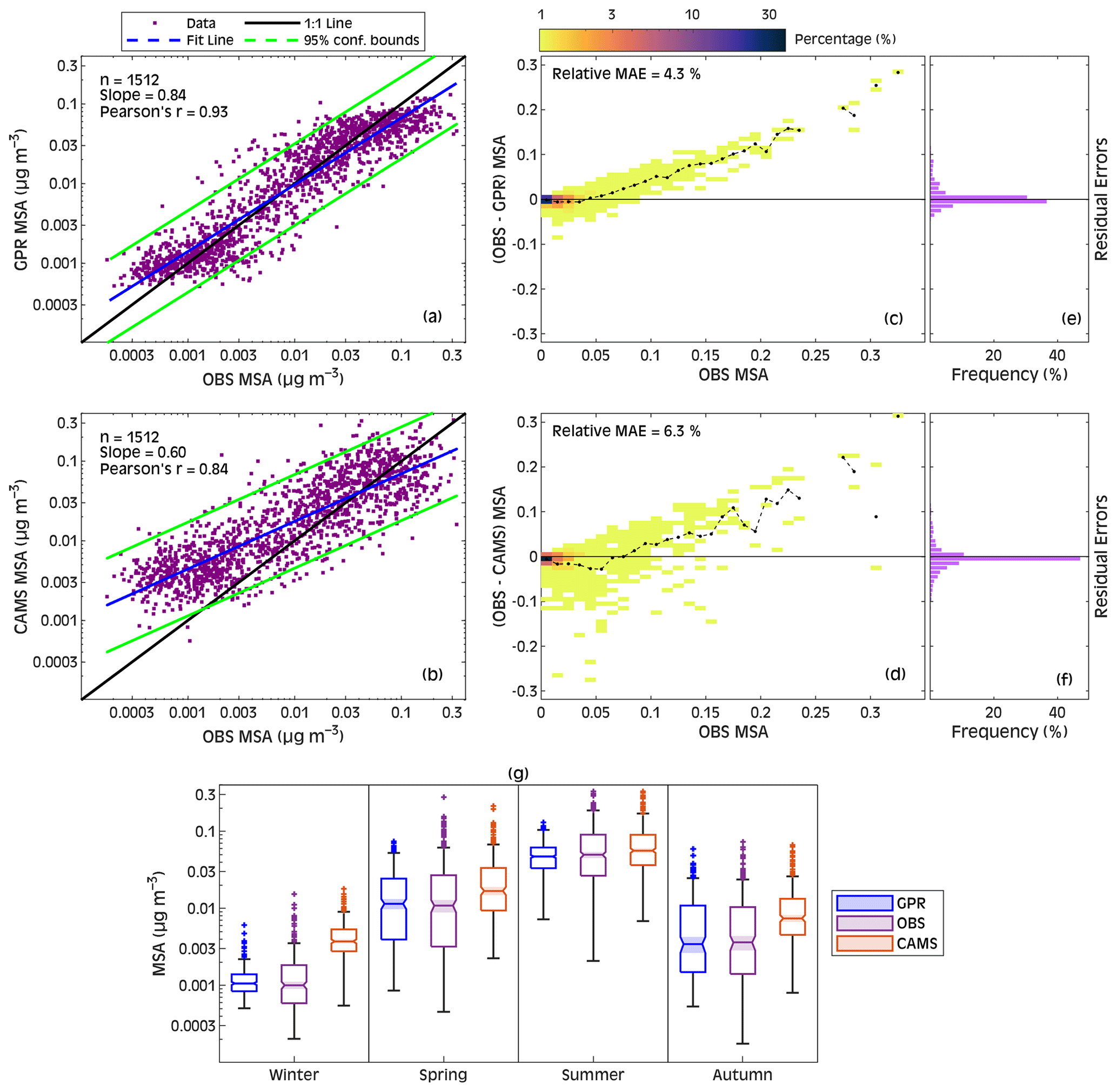
Figure 6 Comparison between observed MSA at the MHD measuring site and both MSA predicted by GPR (a) and MSA extracted from CAMS Reanalysis (b). Panels (c) and (d) present joint probability histograms between observed MSA and residual errors (observed − predicted); the dashed black lines represent the change in MSA residual errors in each bin. MAE is the mean absolute error, and the relative MAE has been calculated as the MAE divided by the range of observed MSA. Panels (e) and (f) show frequency distributions of the residual errors. Panel (g) contains seasonal box charts from different datasets. Each box chart displays the median (line inside of each box), the 1st and 3rd quartiles (bottom and top edges of each box), the minimum and maximum values that are not outliers (whiskers), and any outliers (represented by “+” and computed as values that are more than 1.5 of the interquartile range away from the top or bottom of the box). Box charts whose notches (the shaded region around each median) do not overlap have different medians at the 95 % confidence level.

4.5 Comparison with the Polarstern cruise results

In this section, we present a case study exemplifying how the IPB-MSA&SO₄ datasets can be used. Because the data product represents the concentration of freshly formed sulfur aerosol species and the ML model does not account for atmospheric transport, users must interpret the datasets considering the air mass history. To better clarify the idea, we employed the independent MSA data measured during the Polarstern campaigns in the NA (Huang et al., 2017), which were not used in the training/validation or testing/evaluation of the ML models, and compared them with MSA predicted by GPR. In particular, the MSA predicted by GPR was extracted along air mass BTs arriving at the hourly sites of the ship tracks and then averaged considering a 0 d (no air mass history), 1, 2, and 3 d air mass history. The MSA measurements on Polarstern were performed during four scientific cruises, including two spring seasons (April–May 2011 and April–May 2012) and two autumn seasons (October–November 2011 and October–November 2012). The ship tracks of the cruises from which the data were taken in the present study are shown in Fig. 7. It can be seen that the best match between GPR-simulated MSA and observed MSA occurred when 2 d air masses were considered. At a 2 d air mass history, the slope reached 0.78 and the correlation coefficient reached 0.81 (Fig. 7a–d). Again, as seen in Fig. 7f, GPR MSA is considerably more consistent with observations than CAMS, for which a significant difference with observations (p<0.05) can be appreciated.

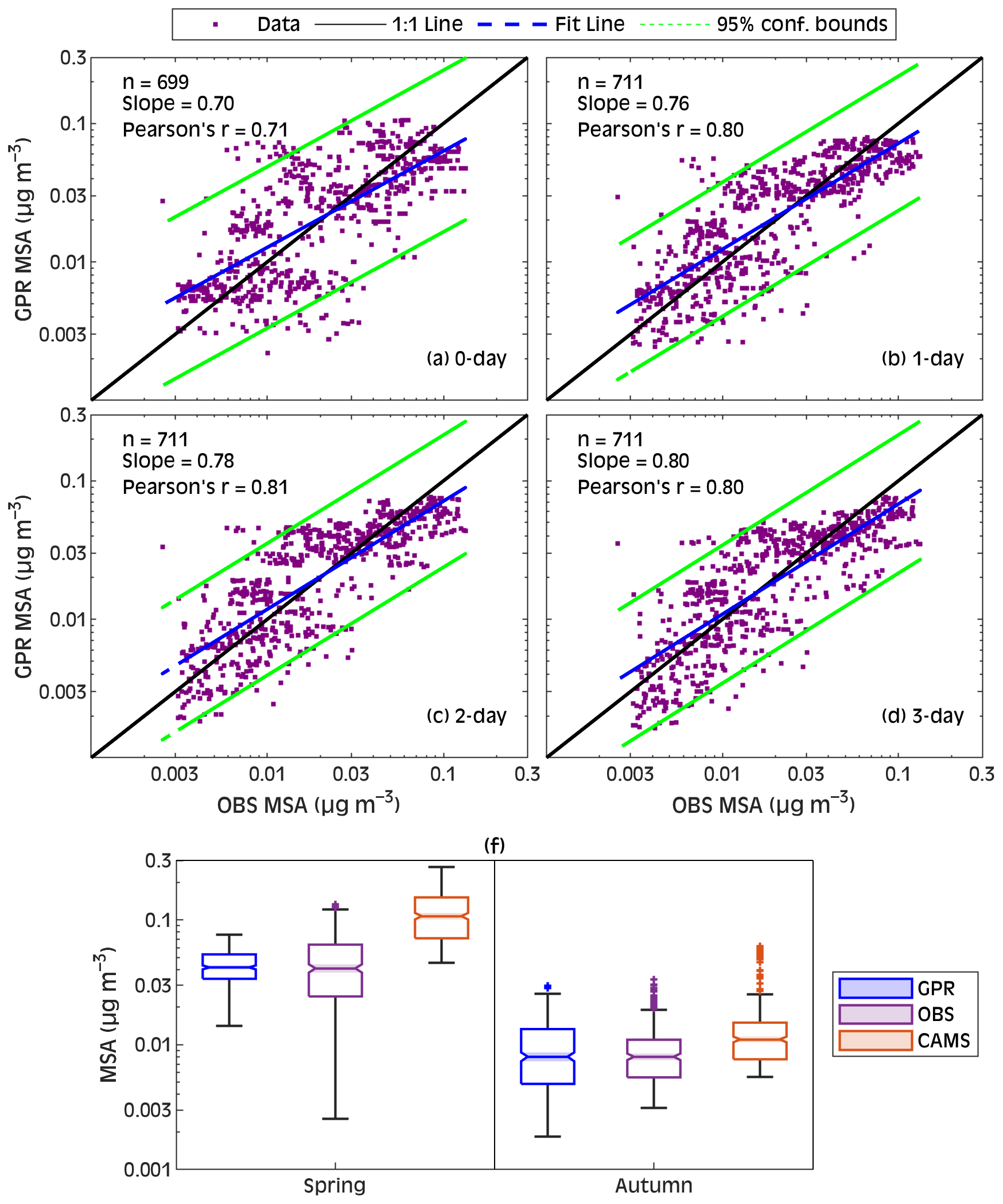
Figure 7 (a) Scatterplots between observed MSA during the Polarstern campaigns (Huang et al., 2017) and predicted MSA by GPR, considering (a) 0 d, (b) 1 d, (c) 2 d, and (d) 3 d air mass history. Panel (f) contains seasonal box charts from different datasets. The features displayed on each box chart are the same as those given in Fig. 6.

4.6 Spatial distributions of MSA and nss-SO${}_{\mathrm{4}}^{=}$

In order to elucidate the geographical distributions of biogenic sulfur aerosol production across the NA domain, the IPB-MSA&SO₄ datasets for the 25 years (1998–2022) were averaged to obtain the climatic annual and monthly distributions of MSA and nss-SO${}_{\mathrm{4}}^{=}$, as illustrated in Figs. 8 and 9. Across the NA domain, the annual average of MSA is 0.016 ± 0.007 µg m⁻³, whereas the annual average of nss-SO${}_{\mathrm{4}}^{=}$ is 0.250 ± 0.077 µg m⁻³ (Table S2). The annual spatial distributions of MSA and nss-SO${}_{\mathrm{4}}^{=}$ exhibit a latitudinal gradient over the majority of the NA area that increases from north to south, except below approximately 35° N, where it increases from west to east. Notwithstanding, the latitudinal gradients are much more evident than longitudinal variations. For instance, MSA grows at a rate of 0.0016 (R²=0.93; p<0.05) µg m⁻³ per degree latitude towards the south and 0.00036 (R²=0.53; p<0.05) µg m⁻³ per degree longitude eastward (it reaches its peak between 20 and 10° W). Furthermore, for each degree southward, nss-SO${}_{\mathrm{4}}^{=}$ increases by 0.0212 (R²=0.96; p<0.05) µg m⁻³, whereas there are no significant changes in nss-SO${}_{\mathrm{4}}^{=}$ with longitude (R²=0.01; p>0.05). The highest concentrations of both components (>90th percentile) are primarily found in the southeast of the domain (in front of the Moroccan coast and the Strait of Gibraltar). Minimum annual concentrations (<10th percentile) are found in northern areas of the domain, particularly in the Labrador Sea and near the shores of Greenland and Iceland.

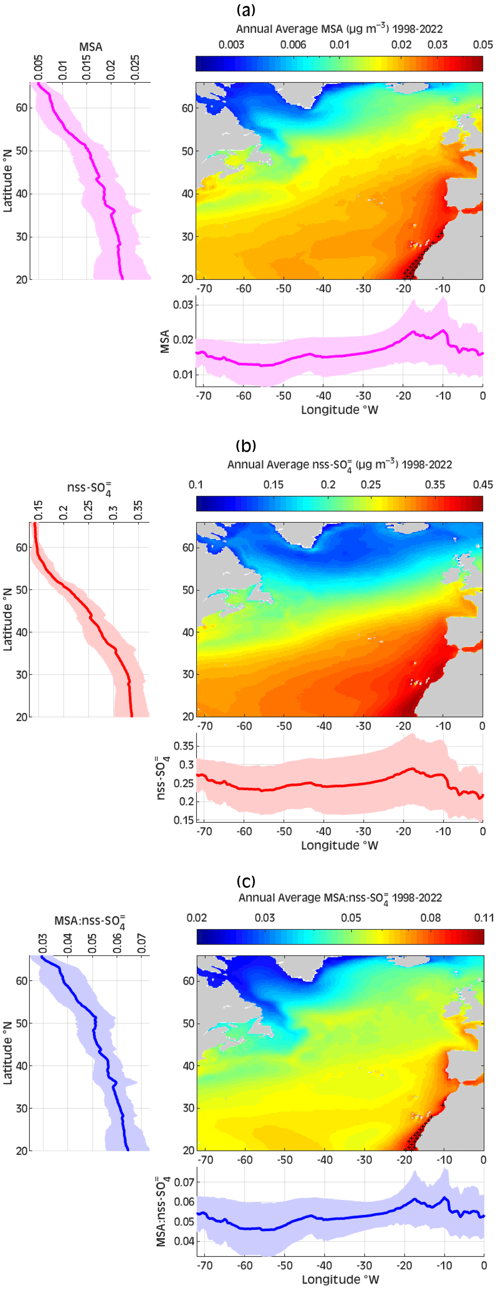
Figure 8 The annual averages of (a) MSA, (b) nss-SO${}_{\mathrm{4}}^{=}$, and (c) $\mathrm{MSA}:\mathrm{nss}-{\mathrm{SO}}_{\mathrm{4}}^{=}$ spatial distributions based on GPR at a 0.25° × 0.25° resolution during the 1998–2022 period. The latitudinal (longitudinal) gradients of each component are displayed in the left (bottom) panels, shaded areas represent ± standard deviations, and the black crosses evidence the extremely high concentrations (more than 3 times the standard deviation plus the annual mean climatology).

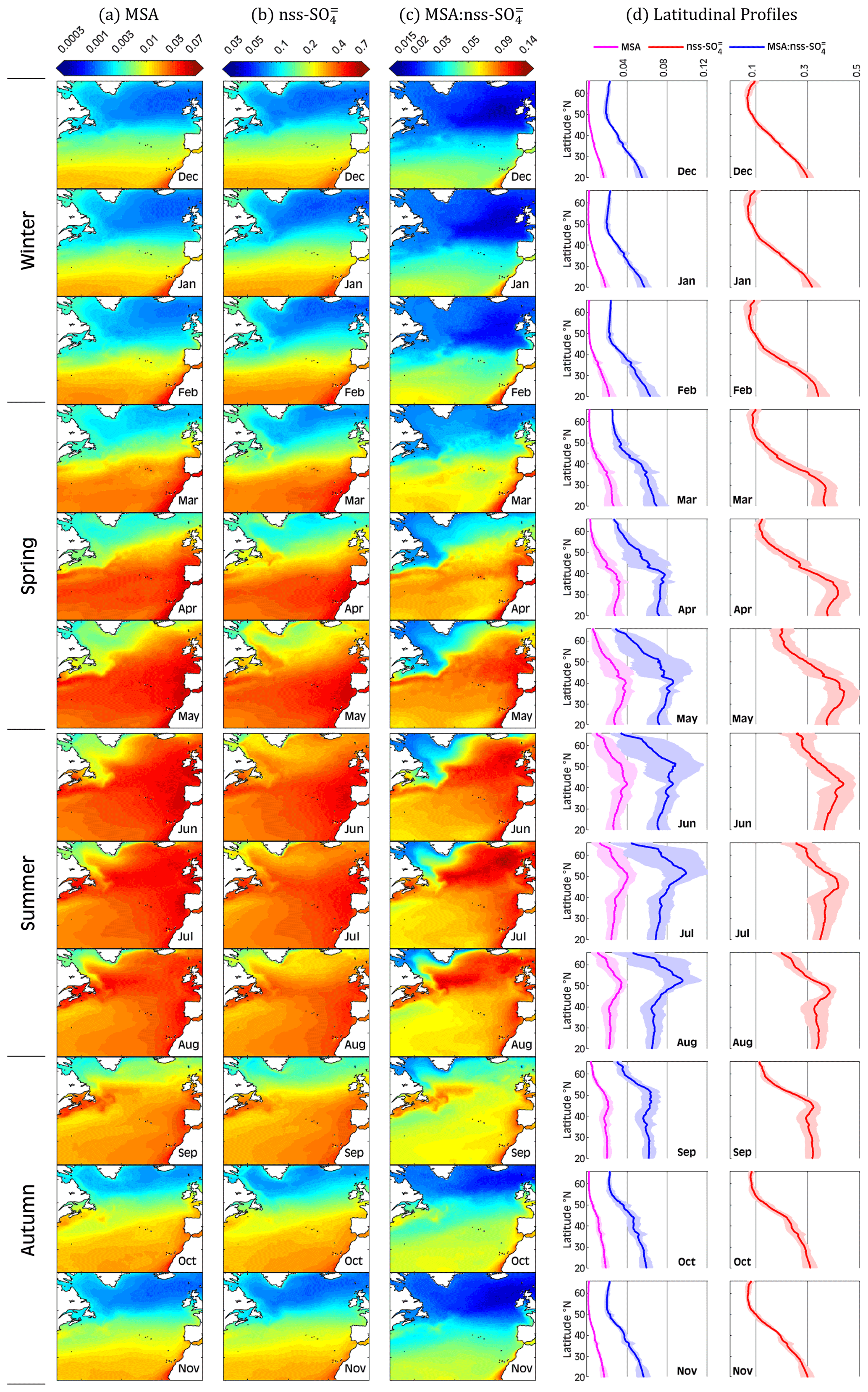
Figure 9 Monthly spatial distributions of (a) MSA, (b) nss-SO${}_{\mathrm{4}}^{=}$, and (c) $\mathrm{MSA}:\mathrm{nss}-{\mathrm{SO}}_{\mathrm{4}}^{=}$ based on GPR over 1998–2022 at a 0.25° × 0.25° resolution. Panel (d) shows monthly latitudinal distributions of each component, with the shaded areas representing ± standard deviations.

The annual average MSA-to-nss-SO${}_{\mathrm{4}}^{=}$ ratio ($\mathrm{MSA}:\mathrm{nss}-{\mathrm{SO}}_{\mathrm{4}}^{=}$) is 0.053 ± 0.012 (Table S2), with a consistent latitudinal gradient increasing southward (rate of change = 0.0028 (R²=0.93; p<0.05) per degree latitude). Lower MSA: nss-SO${}_{\mathrm{4}}^{=}$ values are found in the northwest of the domain, while higher values are apparent in front of the African coast; the ratio is practically constant across the same latitudinal band. It is worth noting that the region with extremely high MSA concentrations and high $\mathrm{MSA}:\mathrm{nss}-{\mathrm{SO}}_{\mathrm{4}}^{=}$ (above the mean + 3 times the standard deviation) is linked to the Canary upwelling system on the northwest African coast. The Canary Current system is one of the world's most productive regions of the ocean, known as eastern boundary upwelling systems (EBUSs) (Chavez and Messié, 2009; Carr, 2001). This may indicate a link between EBUSs and the potential formation of biogenic aerosol in the atmosphere. Previous research has shown how EBUSs changed in response to climate change (Bograd et al., 2023; Sydeman et al., 2014; Bonino et al., 2019), including the trend toward increased upwelling intensity (Wang et al., 2015; García-Reyes et al., 2015); however, little is known about the impact of EBUSs on marine biogenic emissions and the resultant aerosol fluxes. Future studies are needed to address these issues in order to better understand the role of EBUSs in aerosol-climate systems.

Looking at the monthly climatological maps (Fig. 9), it is revealed that MSA and nss-SO${}_{\mathrm{4}}^{=}$ display a gradual southward increase in their concentrations, clearly evident from October to March, resulting in a large difference between the northern and southern parts of the domain. On the contrary, during summer, the concentrations are more homogeneous over the domain (see latitudinal patterns in Fig. 9), still with a tendency toward higher concentrations over the northeastern part of the region. The seasonality of MSA and nss-SO${}_{\mathrm{4}}^{=}$ is evident: the increase in both compounds starts in April, peaks in June–July, and is followed by a gradual decrease in September (Fig. S9, Table S2). The lowest MSA (nss-SO${}_{\mathrm{4}}^{=}$) concentration occurs in December at 0.006 ± 0.005 (0.155 ± 0.079) µg m⁻³, whereas the highest concentration occurs in June at 0.029 ± 0.013 (0.364 ± 0.075) µg m⁻³ (Table S2), consistent with the fact that winter and summer are typically the lowest and highest seasons with respect to biological activity, respectively, for the NA (Mansour et al., 2023a). The coefficient of variation (COV), defined as the ratio between the standard deviation and the mean value, expressed as a percentage at each grid point, is used to assess how much MSA and nss-SO${}_{\mathrm{4}}^{=}$ vary around their mean value in each month; variability increases with a higher COV. The maps (Fig. S10) confirm that the variability in sulfur aerosol species depends strongly on the season: MSA and nss-SO${}_{\mathrm{4}}^{=}$ are mostly stable (small variations) during the winter, whereas most variations occur between April (late spring) and June (early summer) and preferentially over the eastern part of the NA compared with the western part.

$\mathrm{MSA}:\mathrm{nss}-{\mathrm{SO}}_{\mathrm{4}}^{=}$ also exhibits a seasonal pattern, with the lowest (highest) values observed during the winter (summer), as presented in Fig. 9c. July has the highest spatial average of the ratio of 0.077 ± 0.022, while the lowest value of 0.032 ± 0.012 occurs in December (Table S2). Looking at the overall distributions, $\mathrm{MSA}:\mathrm{nss}-{\mathrm{SO}}_{\mathrm{4}}^{=}$ demonstrates a general southward increase, with the exception of summer months. In summer (mainly July and August), $\mathrm{MSA}:\mathrm{nss}-{\mathrm{SO}}_{\mathrm{4}}^{=}$ above 50° N has an opposite trend with respect to the ratio below 50° N. In detail, from north to south, we report a sharp increase in $\mathrm{MSA}:\mathrm{nss}-{\mathrm{SO}}_{\mathrm{4}}^{=}$, maximized around 50° N, followed by an abrupt decrease toward the Equator. A possible explanation for the decline in $\mathrm{MSA}:\mathrm{nss}-{\mathrm{SO}}_{\mathrm{4}}^{=}$ below 50° N is that the reduction is related to an increase in AT caused by warmer air nearing the Equator, in line with observations in the Pacific Ocean (Bates et al., 1992) and with the higher ratio observed in colder (marine polar and arctic) air masses with respect to warmer (marine tropical) air masses at MHD (Ovadnevaite et al., 2014). As a final remark, we report that the summertime low $\mathrm{MSA}:\mathrm{nss}-{\mathrm{SO}}_{\mathrm{4}}^{=}$ below 50° N is linked to a decrease in F_DMS in the same latitudinal zone (Mansour et al., 2023a). Owing to the low DMS emissions, different DMS oxidation patterns may be in competition (Barone et al., 1995); as MSA is formed preferentially through the pathway of OH addition at low temperatures (Shen et al., 2022), the production of MSA may be decreased relative to that of nss-SO${}_{\mathrm{4}}^{=}$ in the warm southern part of the domain, during summer, leading to the observed decrease in $\mathrm{MSA}:\mathrm{nss}-{\mathrm{SO}}_{\mathrm{4}}^{=}$.

5 Data availability

The dataset includes daily MSA and nss-SO${}_{\mathrm{4}}^{=}$ concentrations at a 0.25° × 0.25° spatial resolution over the North Atlantic from January 1998 to December 2022. The data are publicly available in NetCDF format as daily files on the Mendeley Data online repository at https://doi.org/10.17632/j8bzd5dvpx.1 (Mansour et al., 2023b).

6 Conclusions

Marine aerosol data can be obtained from in situ coastal observatories or from shipborne measurements; however, coast observations at individual measurement points are limited with respect to their spatial representativity, while shipborne measurements suffer from limitations in terms of temporal coverage. Understanding the dynamics of marine-derived biogenic sulfur aerosols and their radiative effects, as well as carrying out relevant scientific studies, requires long-term, continuous, high-resolution (both spatial and temporal resolution) datasets. To overcome the limitations of point-based measurements, we combined the in situ observations of sulfur aerosol data at Mace Head and those from NAAMES cruises, as dependent variables, and the sea-to-air DMS flux and ECMWF ERA5 reanalysis meteorological datasets, as independent variables, to investigate the potential of machine learning techniques for the prediction of daily MSA and nss-SO${}_{\mathrm{4}}^{=}$ sea-level concentrations over the North Atlantic. We evaluated five machine learning models (i.e., SVM, DT, RE, GPR, and ANN), considering various sets of hyperparameter optimizations. Our findings demonstrate that the GPR model outperforms other approaches with respect to simulating the concentrations of biogenic sulfur aerosols, capturing up to 86 % and 72 % of the observed variance in daily MSA and nss-SO${}_{\mathrm{4}}^{=}$, respectively. This makes the GPR an effective tool for obtaining trustworthy sea-level MSA and nss-SO${}_{\mathrm{4}}^{=}$ concentrations over the North Atlantic, which may also result in it be successful in other oceanic regions or over the entire global ocean. The impact of the six independent predictors on the simulated MSA and nss-SO${}_{\mathrm{4}}^{=}$ is further evaluated using the GPR partial dependence analysis, which reveals that the relationships between them are multifaceted rather than linear or monotonically varying.

Using the GPR machine learning method, we constructed a novel 0.25° × 0.25° resolution daily gridded dataset of in situ-produced biogenic MSA and nss-SO${}_{\mathrm{4}}^{=}$ concentrations (named IPB-MSA&SO₄) covering the North Atlantic from 1998 to 2022. The dataset represents the sea-level concentrations of MSA and nss-SO${}_{\mathrm{4}}^{=}$ associated with in situ production in the MBL, i.e., the concentration of sulfur aerosol species resulting, in each pixel, from the local biogenic emissions in combination with local atmospheric conditions. Other inputs, such as terrestrial emissions or sinking of sulfur species produced in the free troposphere are not accounted for in the present dataset.

Comparison of the GPR-derived MSA with existing CAMS-EAC4 reanalysis product reveals that our high-resolution dataset accurately reproduces the spatial and temporal patterns of the biogenic sulfur aerosol concentration and has high consistency with the independent observations of the Polarstern cruises' measurements in the Atlantic. The obtained IPB-MSA&SO₄ data were used to analyze the spatiotemporal variations in MSA, nss-SO${}_{\mathrm{4}}^{=}$, and the ratio between them ($\mathrm{MSA}:\mathrm{nss}-{\mathrm{SO}}_{\mathrm{4}}^{=}$). It was found that the monthly concentrations of MSA and nss-SO${}_{\mathrm{4}}^{=}$ across the NA are characterized by a significant southward increase in each month, with the exception of summertime when MSA and nss-SO${}_{\mathrm{4}}^{=}$ displayed more homogeneous spatial patterns with a tendency toward higher concentrations over the northeastern part of the domain. $\mathrm{MSA}:\mathrm{nss}-{\mathrm{SO}}_{\mathrm{4}}^{=}$ exhibits a seasonal variation from winter (low) to summer (high), characterized by a sharp decline from the 50° N parallel toward the Equator mainly in July–August. In general, the atmospheric concentration of sulfur aerosol species tends to be more stable in winter, whereas wider variations are associated with late-spring and early summertime and more with the eastern part of the domain than with the western part.

More in-depth analyses can be conducted based on the presented biogenic sulfur aerosol concentration dataset, which could help further the understanding of marine-aerosol–cloud interactions. For instance, we evidence that the Canary eastern upwelling system emerges from the dataset as a hot spot of high sea-level MSA concentrations and high $\mathrm{MSA}:\mathrm{nss}-{\mathrm{SO}}_{\mathrm{4}}^{=}$ values. Such a finding is worth further investigation and may shed light on the role of EBUSs in the production of biogenic marine aerosols and on their climate relevance.