Global anthropogenic emissions (CAMS-GLOB-ANT) for the Copernicus Atmosphere Monitoring Service simulations of air quality forecasts and reanalyses

Anthropogenic emissions are the result of many different economic sectors, including transportation, power generation, industrial, residential and commercial activities, waste treatment and agricultural practices. Air quality models are used to forecast the atmospheric composition, analyze observations and reconstruct the chemical composition of the atmosphere during the previous decades. In order to drive these models, gridded emissions of all compounds need to be provided. This paper describes a new global inventory of emissions called CAMS-GLOB-ANT, developed as part of the Copernicus Atmosphere Monitoring Service (CAMS; https://doi.org/10.24380/eets-qd81, Soulie et al., 2023). The inventory provides monthly averages of the global emissions of 36 compounds, including the main air pollutants and greenhouse gases, at a spatial resolution of 0.1° × 0.1° in latitude and longitude, for 17 emission sectors. The methodology to generate the emissions for the 2000–2023 period is explained, and the datasets are analyzed and compared with publicly available global and regional inventories for selected world regions. Depending on the species and regions, good agreements as well as significant differences are highlighted, which can be further explained through an analysis of different sectors as shown in the figures in the Supplement.

1 Introduction

The design of mitigation policies for both pollutants and greenhouse gases, as well as verification of the efficiency of these policies, relies on chemistry-climate and chemistry-transport models. In order to provide accurate results, these models require good knowledge of the emissions inventories of many atmospheric compounds. These inventories provide the necessary information to calculate the concentrations of atmospheric species emitted from natural and anthropogenic processes: these species can then be affected by chemical transformations and transport processes, and lead to the formation of other chemical species. Accurate knowledge of the spatial and temporal distribution of primary emissions is therefore essential to quantify the impact of surface emissions on the distribution of atmospheric pollutants and greenhouse gases.

During the past decades, many emission inventories have been developed at the global and regional scales, as detailed in Sect. 2 and in Granier et al. (2023). In general, surface emissions are calculated as the product of activity rates, emission factors and other factors depending on the type of source. Such data, for example, activity rates, take a long time to collect, and the development of inventories is also a time-consuming effort. Therefore, most inventories do not provide emissions for the most recent years.

As part of Copernicus (https://www.copernicus.eu; last access: April 2024), the European Union's Earth observation program, the Copernicus Atmosphere Monitoring Service (CAMS: https://atmosphere.copernicus.eu; last access: April 2024; Peuch et al., 2022) delivers near-real-time analyses on a daily basis and forecasts of the atmospheric composition at the global scale (Flemming et al., 2015). CAMS delivers as well a global reanalysis, which provides consistent multi-annual global datasets of atmospheric composition since the year 2003 (Inness et al., 2019). The forecasts and reanalysis provide three-dimensional fields of aerosols, gaseous chemical species and greenhouse gases. In order to provide these forecasts and reanalysis, the CAMS chemistry-transport models require up-to-date surface emissions.

None of the currently publicly available inventories, such as the ones described in Sect. 2 and in Granier et al. (2023), provide the emissions required by the CAMS forecasts and reanalysis: either they cover a too short period for the reanalysis or they do not provide emissions for the recent and current years, as required for global forecasts. Therefore, a new dataset called CAMS-GLOB-ANT has been developed during the past few years, and it includes the emissions for air pollutants and greenhouse gases for real-time forecasts at the spatial and temporal resolution required by the CAMS and other chemistry-climate models. This paper describes the existing datasets (Sect. 2) used in the methodology to develop CAMS-GLOB-ANT (Sect. 3) and compares the dataset with other inventories (Sect. 4), as well as provides information from studies done using the CAMS-GLOB-ANT dataset. Section 5 includes information on how to get access to the dataset.

2 Datasets used in the development of CAMS-GLOB-ANT

The version of the CAMS-GLOB-ANT global anthropogenic emissions described in this paper is version 5, which is based on the Emissions Database for Global Atmospheric Research (EDGARv5), the emissions provided by the Community Emissions Data System (CEDS; O'Rourke et al., 2021a, b) which are used for the extrapolation of the emissions to the most recent years, the temporal profiles from the CAMS-GLOB-TEMPO dataset and the ship emissions from the CAMS-GLOB-SHIP dataset. Each of these inventories is described in the following subsections.

2.1 EDGAR emissions

EDGAR, the Emissions Database for Global Atmospheric Research (https://edgar.jrc.ec.europa.eu/; last access: April 2024), is developed at the Joint Research Center (JRC) in Italy. EDGAR provides emissions as national totals and grid maps at 0.1° × 0.1° resolution at the global level, with yearly and monthly averages. The emissions are calculated using a technology-based emission factor approach for the different countries and for 27 different sectors: the list of the sectors included in EDGARv5 is shown in Table S1 in the Supplement.

The methodology used for the EDGAR emissions is described in Crippa et al. (2018, 2021) and online (https://edgar.jrc.ec.europa.eu/methodology; last access: April 2024). We have used here version 5 of EDGAR, which provides for the 1970–2015 period and gridded emissions for greenhouse gases (CO₂, CH₄ and N₂O), as well as for air pollutants, i.e., CO, NO_x, non-methane volatile organic compounds (NMVOCs), NH₃, SO₂, black carbon (BC) and organic carbon (OC). The national totals and gridded emissions for the different years and sectors are publicly available at: https://edgar.jrc.ec.europa.eu/dataset_ap50 (last access: April 2024).

The emissions for 25 speciated volatile organic compounds are also provided by EDGAR up to the year 2012 (https://edgar.jrc.ec.europa.eu/dataset_ap432_VOC_spec; last access: April 2024), following the methodology described in Huang et al. (2017).

2.2 CEDS emissions

CEDS, the Community Emissions Data System (https://www.pnnl.gov/projects/ceds; last access: April 2024), is developed at the Joint Global Research Institute in Maryland, USA. CEDS emissions are developed within an open-source framework that produces annual emission estimates for research and analysis. The methodology used to derive the global emissions is detailed in Hoesly et al. (2018) and in McDuffie et al. (2020).

We have used the version of CEDS from O'Rourke et al. (2021a) which provides global emissions at a 0.5° × 0.5° on a monthly basis for the following species: SO₂, NO_x, BC, OC, NH₃, NMVOCs, CO, CO₂, CH₄ and N₂O. This dataset is available at https://doi.org/10.25584/PNNLDataHub/1779095 (Smith et al., 2019, last access: April 2024). The country emissions are given for 57 sectors from 1750 to 2019 (O'Rourke et al., 2021b) and are available at https://doi.org/10.5281/zenodo.4737769 (O'Rourke et al., 2021a). The sectors included in the CEDS emissions by country are given in Table S1.

2.3 CAMS-GLOB-SHIP emissions

For the ship emissions, we have used the CAMS-GLOB-SHIP, version 3.1, dataset. These emissions are generated by the Ship Traffic Emission Assessment Mode (STEAM3; Johansson et al., 2017), which uses global vessel activity from 2014 to 2018, constructed from both terrestrial and satellite data from automatic identification system (AIS) transponders, where all vessels larger than 300 t and all passenger ships report their position with intervals of a few seconds. It should be noted that the coverage of inland shipping data may be poor, because the use and coverage of AIS in inland waterways is not yet mandatory.

The earlier years, 2000–2013, have been backcasted based on 2016 activity data and using scaling factors taking into account fleet size growth, the lower energy efficiency and smaller ship size in previous years. These scaling factors are applied separately for various shipping segments.

Disruptions, like the COVID-19 pandemic, are considered, because the underlying activity data are based on observed ship locations. Changes in environmental regulation of the shipping sector have been included at global and regional levels. These changes include the establishment of emission control areas (ECAs) for SO_x and NO_x in the Baltic Sea, North Sea and North America, as well as Chinese domestic ECAs and vessel type specific rules for ships operating in European seas, as defined by the International Maritime Organization (https://www.imo.org/en/OurWork/Environment/Pages/ Emission-Control-Areas-(ECAs)-designated-under-regulation-13-of-MARPOL-Annex-VI-(NOx-emission-control).aspx; last access: April 2024). A global sulfur cap (a limit on the sulfur content in the fuel oil used on board ships) became effective on 1 January 2020 which decreased SO_x and PM emissions, but the ECA regions, which implemented those rules several years before 2020, were unaffected by the cap. The CAMS-GLOB-SHIP emissions are provided for several chemical compounds, such as CO₂, CO, NO_x, NMVOCs, BC, OC and SO₂.

2.4 CAMS-GLOB-TEMPO temporal profiles

The CAMS-GLOB-ANT monthly variability is implemented using monthly averaged profiles from the CAMS-GLOB-TEMPO dataset, described in Guevara et al. (2021): the monthly temporal profiles used in CAMS-GLOB-ANT are available on the ECCAD database (https://eccad.aeris-data.fr; last access: April 2024). These temporal profiles consider the primary atmospheric pollutants, NO_x, SO₂, NMVOCs, NH₃, CO and the greenhouse gases CO₂ and CH₄, for the following sectors: energy, industry, road transportation, residential and agriculture (livestock, soil and agricultural waste burning), which have a direct correspondence with the sector classification considered in CAMS-GLOB-ANT (Table S1). For the sectors not considered in CAMS-GLOB-TEMPO, the EDGARv5 monthly profiles are used.

The temporal profiles are available at a 0.1° × 0.1° spatial resolution. These temporal profiles are based on statistical information, such as electricity production statistics or measured traffic counts, linked to emission variability at national and regional levels. Parameterizations accounting for meteorological conditions and sociodemographic factors are taken into account in the temporal profiles, including the use of a heating degree day approach. An example of the monthly temporal weights for the residential sector are shown for Madrid (Spain) and Capetown (South Africa) from 2000 to 2020 in Fig. 1. The reported seasonality illustrates the role of meteorological conditions on the temporal variation in the residential emissions. For instance, the three largest peaks computed for Madrid in February 2015, January 2017 and January 2019 coincide with the occurrence of three unusual cold spell and snowfall events that affected this region.

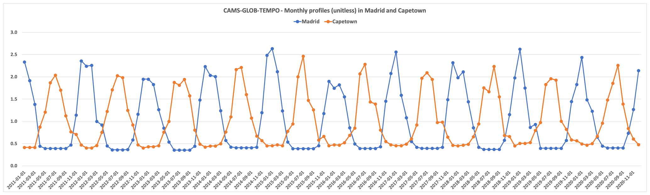
Figure 1 Monthly weights from CAMS-GLOB-TEMPO in Madrid (Spain) and Capetown (South Africa) for the residential sector.

We have used the most recent version of CAMS-GLOB-TEMPO, i.e., version 3.1, which provides temporal profiles from 2000 to 2020. For all the years after 2020, the 2020 monthly temporal profiles have been used.

3 Methodology used for the development of CAMS-GLOB-ANT version 5

3.1 Definition of the sectors

CAMS-GLOB-ANT version 5 provides anthropogenic emissions for 17 sectors and 35 species: CO₂ (divided into short organic cycle (released by combusting biofuels, agricultural waste burning or field burning) and excluding the short cycle), CH₄, N₂O, NO_x, NMVOCs, SO₂, BC, OC, NH₃ and 25 speciated volatile organic compounds. In order to calculate the emissions for the full 2000–2023 period for these sectors, a harmonization and grouping of the sectors of the EDGARv5 and CEDS datasets was performed. The sectors used in CAMS-GLOB-ANT are detailed in Table S1, and the corresponding sectors in the EDGARv5 and CEDS inventories are shown as well in this table. The sectors have been chosen such that they represent the main anthropogenic activities corresponding to power generation, industrial activities, fuel operations, different modes of transportation, residential, agriculture activities and waste management. They have also been chosen such that they are compatible with the definition of the sectors of the European dataset CAMS-REG (Kuenen et al., 2022). The sectors considered for the emissions of each of the 25 speciated volatile organic compounds considered in the inventory are indicated in Table S2.

3.2 Extrapolation of the emissions to the most recent years

In order to obtain emissions that can be used in global forecasts and long-term reanalyses, it is necessary to extrapolate the emissions to the most recent years and months. The EDGARv5 emissions are available until 2015 and the CEDS emissions are available up to 2019. We have used EDGARv5 emissions as a basis for the CAMS emissions, as their spatial resolution is 0.1° × 0.1°, which is the resolution of the emissions required by the CAMS global forecasts. The CEDS emissions are used for the extrapolation of the emissions up to the current year (i.e., 2023 at the time of writing).

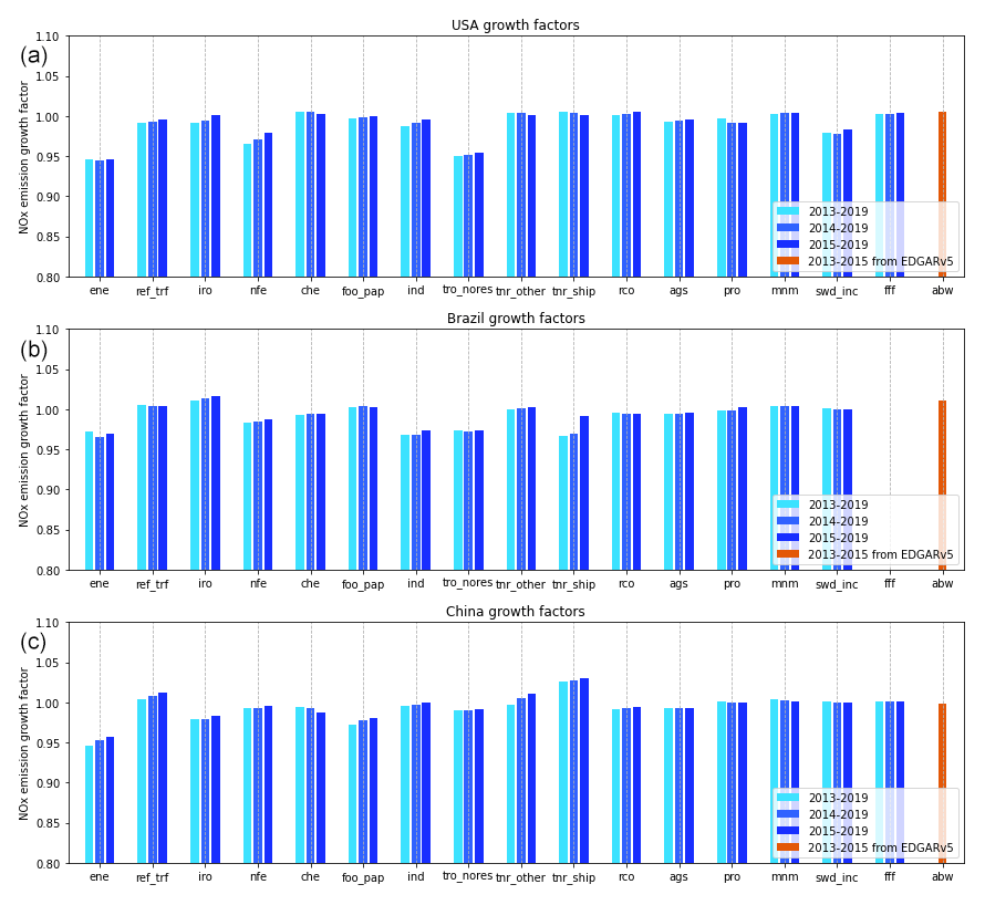
Figure 2 Relative changes in the emissions in the USA (a), Brazil (b) and China (c) for different periods and different sectors.

For this extrapolation, we have first grouped the CEDS emissions for each species in order to obtain the totals emitted for each country for the sectors included in the CAMS-GLOB-ANT dataset, following Table S1. The relative change in the emissions for each country, species and sector for the 2013–2019, 2014–2019 and 2015–2019 periods in the CEDS emissions was then calculated as shown in Fig. 2, which displays the results for three countries, i.e., the USA, Brazil and China, for the emissions of nitrogen oxides. As shown by these figures, the changes in the emissions for the three considered periods are very close, and it was decided to use the 2014–2019 changes in the emissions for the extrapolation to the most recent years.

After grouping the CEDS emissions in order to match EDGARv5 sectors as shown in Table S1, we calculated a factor called the “growth factor” to quantify the change in the emissions, defined as

$$\begin{array}{}\text{(1)}& q={\left({\displaystyle \frac{c_{t_f}}{\text{mean}\left(c_{t_i\to t_f}\right)}}\right)}^{\frac{\mathrm{1}}{t_f-t_i}},\end{array}$$

where q is the dimensionless growth factor, $c_{t_f}$ is the emission for each country in 2019 (t_f) and $c_{t_i}$ is the emission for each country in 2014 (t_i).

For three EDGARv5 sectors, there is no equivalent sector in the CEDS emissions: “non-ferrous metal production” (nfe), “agriculture waste burning” (awb) and “road transportation with resuspension” (tro_res). For the nfe and awb sectors, the growth factors are calculated on the basis of the 2013–2015 EDGARv5 values. For the sector “road transportation with resuspension” the same growth factor as for the road transportation sector is used.

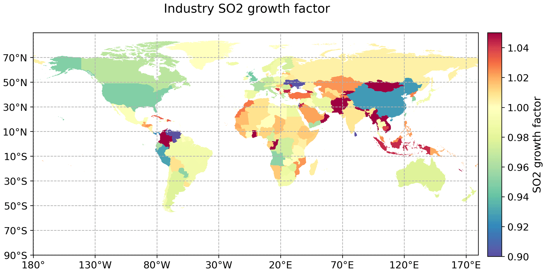
Figure 3 Growth factor for the industry sector used to extrapolate SO₂ emissions.

An example of the growth factor for the industry sector for the SO₂ emissions is shown in Fig. 3: this figure highlights the different patterns of recent changes in the emissions in the different countries of the world.

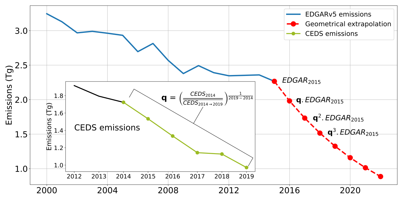
Figure 4 Schematic view of the methodology used to calculate the CAMS-GLOB-ANT emissions for the most recent years.

The emissions at a 0.1° × 0.1° resolution for each species and sector for the years after 2015 are then calculated following a geometric progression, by applying the growth factor as the common ratio for all the grid points in each country. Figure 4 presents a schematic view of the methodology.

Figure 5 Growth factor for the NMVOC species for Germany.

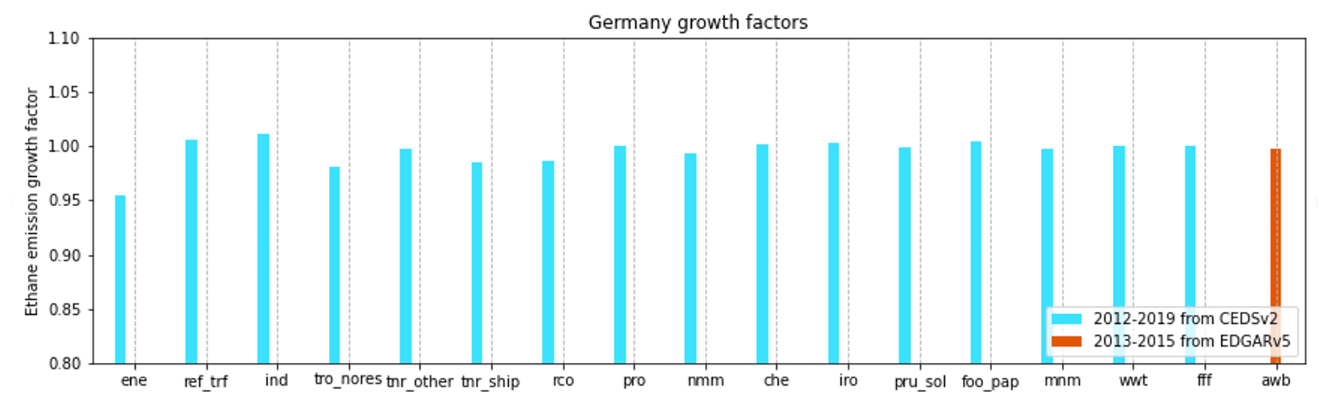
In EDGARv5, as indicated above, the emissions of speciated VOCs are available until 2012 (Huang et al., 2017). The extrapolation of the speciated VOCs is based on the calculation of the growth factor for the NMVOC emissions from CEDS over the 2012–2019 period. An example of the growth factor for Germany is shown in Fig. 5. This growth factor is applied to all the speciated VOCs provided by EDGARv5. As indicated above, the agricultural waste sector is not included in CEDS. For this sector, we have used the growth factor calculated over the 2013–2015 period for the NMVOC species from EDGARv5.

3.3 Aircraft emissions

We have developed the aircraft emissions on the basis of the CEDS aircraft emission data described in Hoesly et al. (2018). For the years up to 2014, the emissions are taken from CEDS, which provides aircraft emissions for CO₂, CH₄, N₂O, CO, NMVOCs, BC, OC, NH₃ and SO₂. After 2014, a linear extrapolation using the trends calculated for the period 2012–2014 is applied to obtain the emissions for the most recent years. The resulting dataset is CAMS-GLOB-AIR version 2.1, providing emissions from aircraft from 2000 to 2023, for 25 levels. The altitude of each of these levels is given in Table S3.

To be consistent with VOC speciation of surface anthropogenic emissions, the emissions of speciated VOC emissions from aircraft in CAMS-GLOB-AIR are based on the speciation described by Huang et al. (2017) for different emission sectors. We calculated the ratios of the emissions of each individual VOC to the total NMVOC species for each of the two altitude levels (landing/taking off and cruise altitudes) in the EDGAR dataset, at a 0.1° × 0.1° horizontal resolution. The ratios for the landing/taking off level were then applied to the first two levels (0.305 and 0.915 km) of the CAMS-GLOB-AIR NMVOC species to get the aircraft emissions of each individual VOC. The ratios for the cruise altitude were applied to all the other levels indicated in Table S3 to obtain the emissions for the rest of the altitudes considered.

4 Results: the CAMS-GLOB-ANT version 5.3 emissions

The CAMS-GLOB-ANT version 5.3 emissions have been obtained using the methodology indicated in the previous sections, i.e., the extrapolation to 2023, the application of the CAMS-GLOB-TEMPO temporal profiles and the use of the CAMS-GLOB-SHIP emissions for ships. The results discussed in this paper will mainly focus on the version 5.3 emissions.

It should be noted that the CAMS-GLOB-ANT version 5.3 emissions do not take into account the impact of the 2020 significant changes in emissions related to the lockdowns implemented by many countries to fight the COVID-19 pandemic. Another dataset, called CONFORM (COVID-19 adjustmeNt Factors fOR eMissions) and described by Doumbia et al. (2021), provides adjustment factors at the same spatial resolution as the CAMS-GLOB-ANT emissions. The CONFORM adjustment factors are available for several sectors compatible with the CAMS-GLOB-ANT emissions. The CONFORM factors have not been implemented in the CAMS-GLOB-ANT dataset in order to allow modelers to perform sensitivity studies, such as studies of the impact of the COVID-19 lockdowns on the global atmospheric composition.

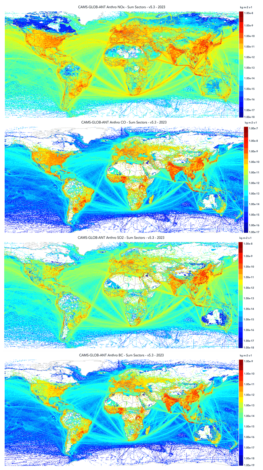
Figure 6 The 2023 annual average of the surface emissions (in kg m⁻² s⁻¹) of NO_x (top left), CO (second from top), SO₂ (third from top) and BC (bottom).

Figure 7 Relative change from 2000 in the global total emissions of several species.

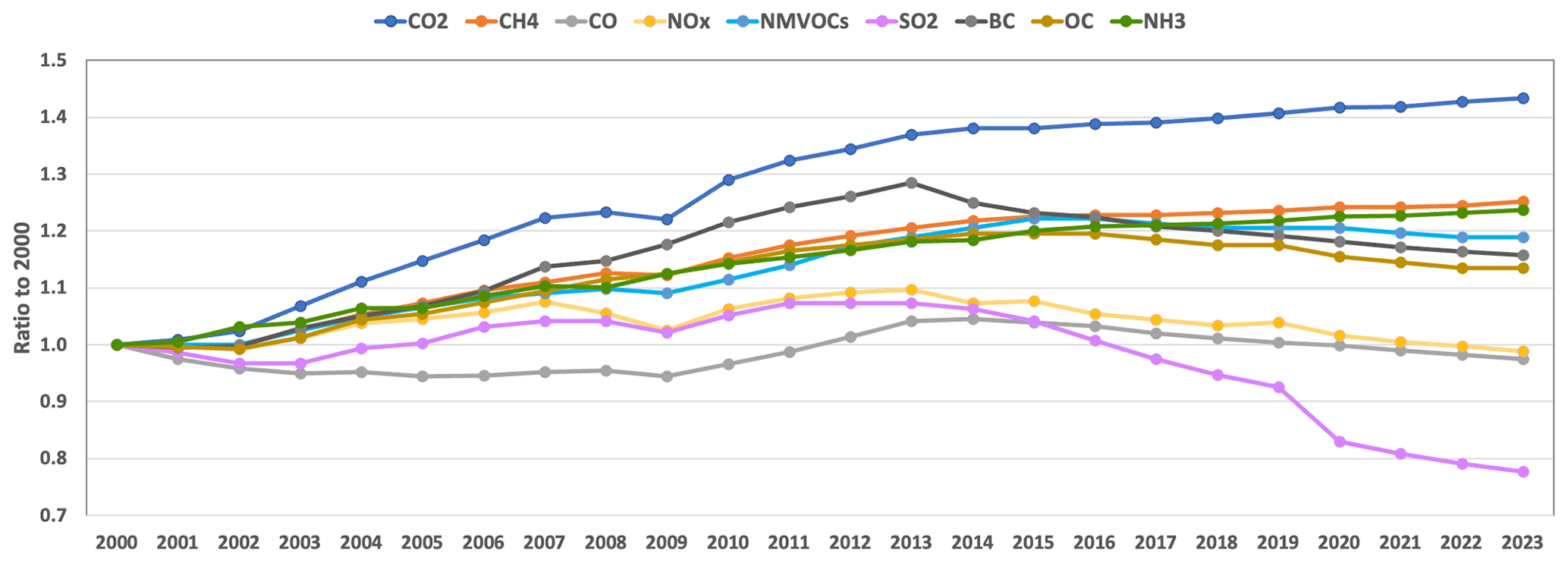
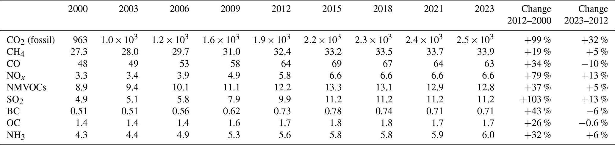
The CAMS-GLOB-ANT_v5.3 inventory provides emissions as monthly averages at a 0.1° × 0.1° spatial resolution in latitude and longitude. The spatial distribution of the yearly averaged emissions for CO, NO_x, NMVOCs, SO₂, BC and OC are shown in Fig. 6. Relative changes in the annual global emissions since 2000 are shown in Fig. 7: the relative change since 2000 is plotted for CO₂ (sum of CO₂_excluding_short_cycle and short_cycle), CH₄, CO, NO_x, NMVOCs, SO₂, BC, OC and NH₃. For species such as CO₂, CH₄ and NH₃, a constant increase is seen for the past two decades. For the other species, a change in the trend (i.e., a decrease in the emissions) is shown around the years 2011–2014.

Table 1 Global totals emitted (in Tg yr⁻¹) for selected species and associated percentage changes. CO₂ (fossil) corresponds to the CO₂ species, excluding short cycle. The NO_x emissions are reported as NO (M=30.01 g mol⁻¹).

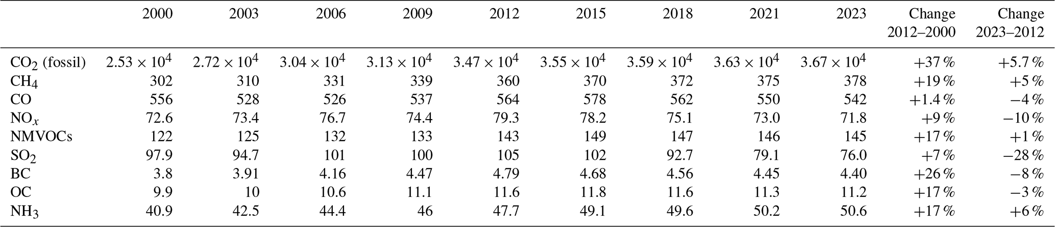
This feature is also shown in Table 1, which indicates the global totals emitted for the same compounds as in Fig. 7 for 2000, 2003, 2009, 2012, 2015, 2018, 2021 and 2023, together with the trends from 2000 to 2012 and from 2012 to 2023. Even for the species for which a constant increase is seen, the trends after 2012 are significantly lower than before 2012. For CO, NO_x, SO₂, BC and OC, the emissions decrease after 2012 as a result of the implementation of several measures to limit the emissions of pollutants. These changes depend strongly on the regions and sectors, as discussed further in the following sections.

In order to better identify the reasons for the changes in the global total emissions from 2000, Tables S4 and S5 indicate the global totals emitted for several species and four groups of sectors for 2000, 2012 and 2023, as well as the 2000–2012 and 2012–2023 changes. Table S4 indicates the values for transportation (sum of road, non-road and ship transportation), and energy + industrial activities (sum of the sectors power generation, refineries, industrial processes, fugitive and solvents), while Table S5 considers the emissions for the residential sector and agriculture/waste (livestock, soils, waste burning and solid waste–waste water). For the global scale, these tables show that the decrease in the emissions or in the trends after 2012 are mostly due to changes in two sectors, transportation and energy + industrial activities. More details on the changes in the emissions for the different sectors will be given in the next section, which will focus on different world regions and countries.

5 Analysis of the CAMS-GLOB-ANT emissions and comparisons with other datasets

This section will analyze the changes in the emissions of CO, NO_x, NMVOCs, SO₂, NH₃, BC and OC for the regions for which regional inventories are available, i.e., western Europe, central Europe, the USA, China and India. The countries in each of the western and central European regions are indicated in Table S6. The changes in the total emissions for each of these regions from 2000 to 2012 and from 2012 to 2023 are shown in Fig. 8. This figure shows significant differences between the trends in all species between the two periods.

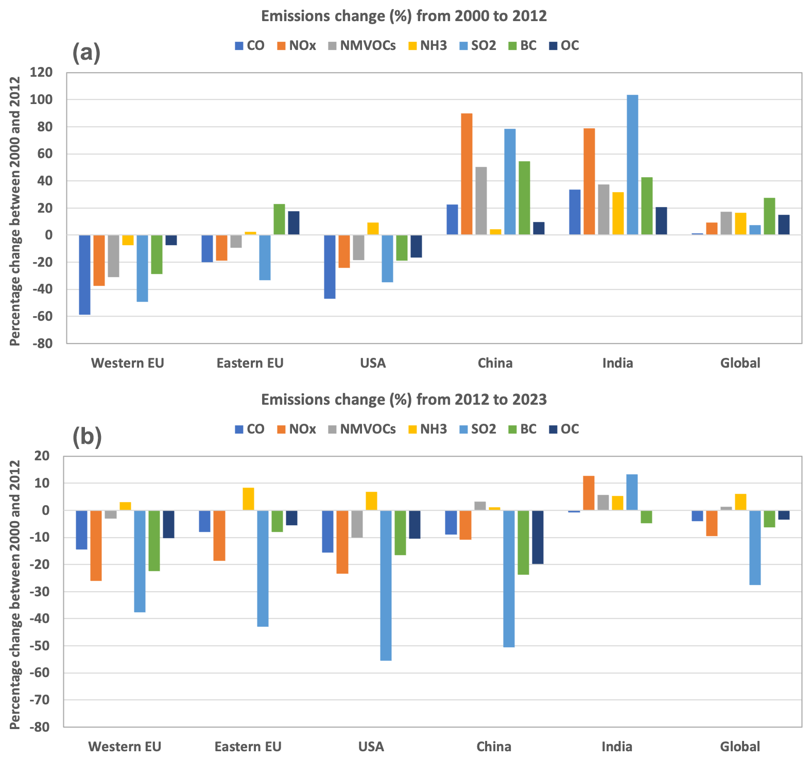
Figure 8 Percentage change in the emissions of CO, NO_x, NMVOCs, NH₃, SO₂, BC and CO from 2000 to 2012 (a) and 2012 to 2023 (b).

These changes will be discussed in more detail in the following sections. Comparisons will be performed using both regional inventories when available and the following global inventories: EDGAR version 5, EDGAR version 6 (published after the development of CAMS-GLOB-ANT version 5.3), CEDS (described in Sect. 2) and HTAP version 3 (Crippa et al., 2023, and https://edgar.jrc.ec.europa.eu/dataset_htap_v3; last access: April 2024). EDGAR and CEDS calculate the emissions on the basis of activity data and emission factors, while the HTAP dataset is based on a mosaic approach, and uses emissions reported by countries and regions when available. ECLIPSE version 6 (https://previous.iiasa.ac.at/web/home/research/researchPrograms/air/ECLIPSEv6b.html; last access: April 2024) is based on future scenarios after 2000. The older dataset called MACCity (Granier et al., 2011), based on a future scenario (RCP8.5; Riahi et al., 2011) after 2005, is also included in these comparisons as these emissions are used in the current CAMS reanalysis (Inness et al., 2019).

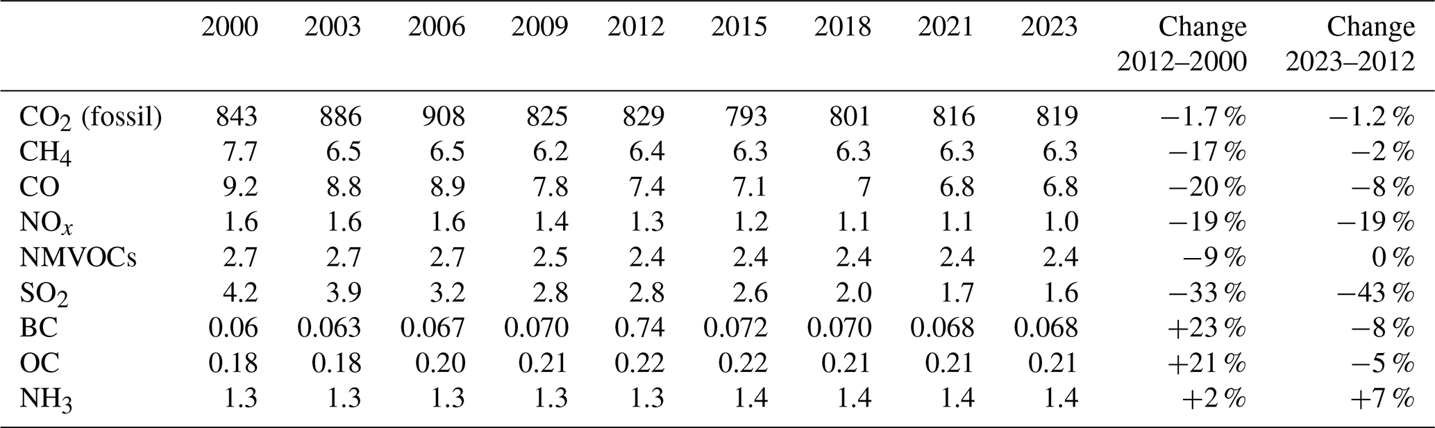
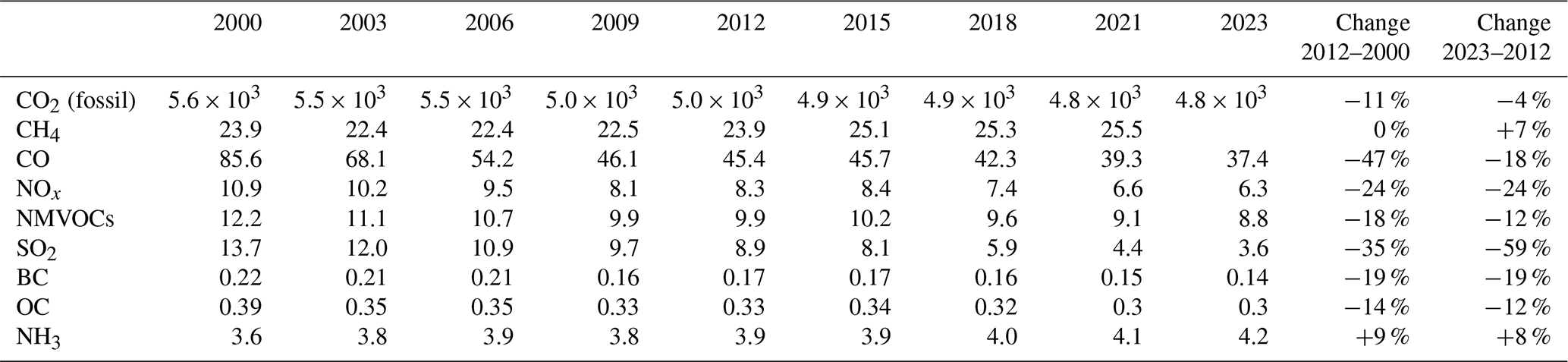
Table 2 Totals emitted in Tg yr⁻¹ and associated percentage changes for western Europe. The values for the NO_x emissions are given in Tg NO_x (as NO) yr⁻¹.

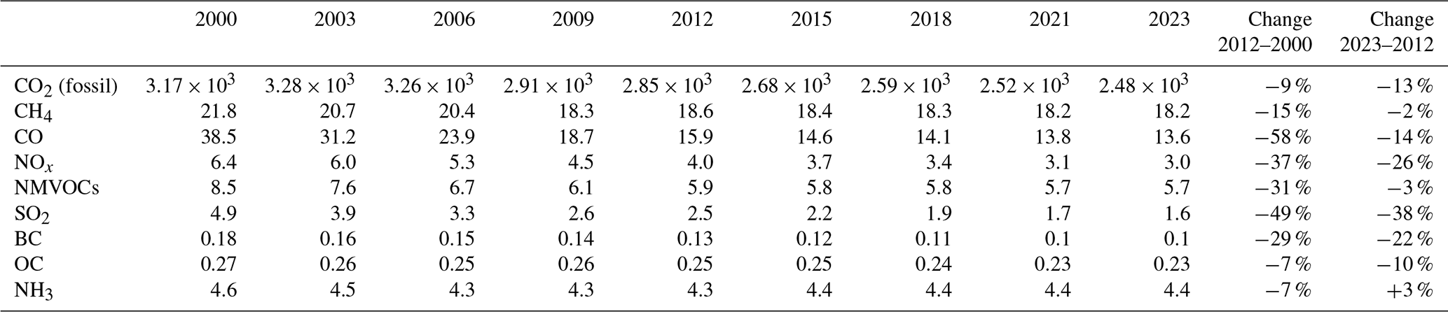
Table 3 Totals emitted in Tg yr⁻¹ and associated percentage changes for central Europe. CO₂ (fossil) corresponds to the CO₂ species, excluding short cycle. The values for the NO_x emissions are given in Tg NO_x (as NO) yr⁻¹.

5.1 Western and central Europe

As shown in Fig. 8, the emissions of CO, NO_x, NMVOCs, SO₂ and BC have decreased significantly in western and central Europe since 2000, while NH₃ and OC do not show a similar pattern. Tables 2 and 3 show the totals emitted for a few species for the same years as in Fig. 8, and the corresponding percentage changes for western and central Europe, respectively.

Large decreases in the emissions are found for the two 2000–2012 and 2012–2021 periods for all species, with the smallest changes for CO₂, OC and NH₃ for both periods, and a slight increase in the NH₃ emissions in the past decade: for NH₃, the rather constant emissions during the full period are related to slight changes in the main contributor of these emissions, i.e., agriculture practices. Figure S1 in the Supplement shows, for western Europe, the changes in the emissions for the different sectors considered for CO, NO_x, NMVOCs and SO₂, i.e., the species which show the largest changes.

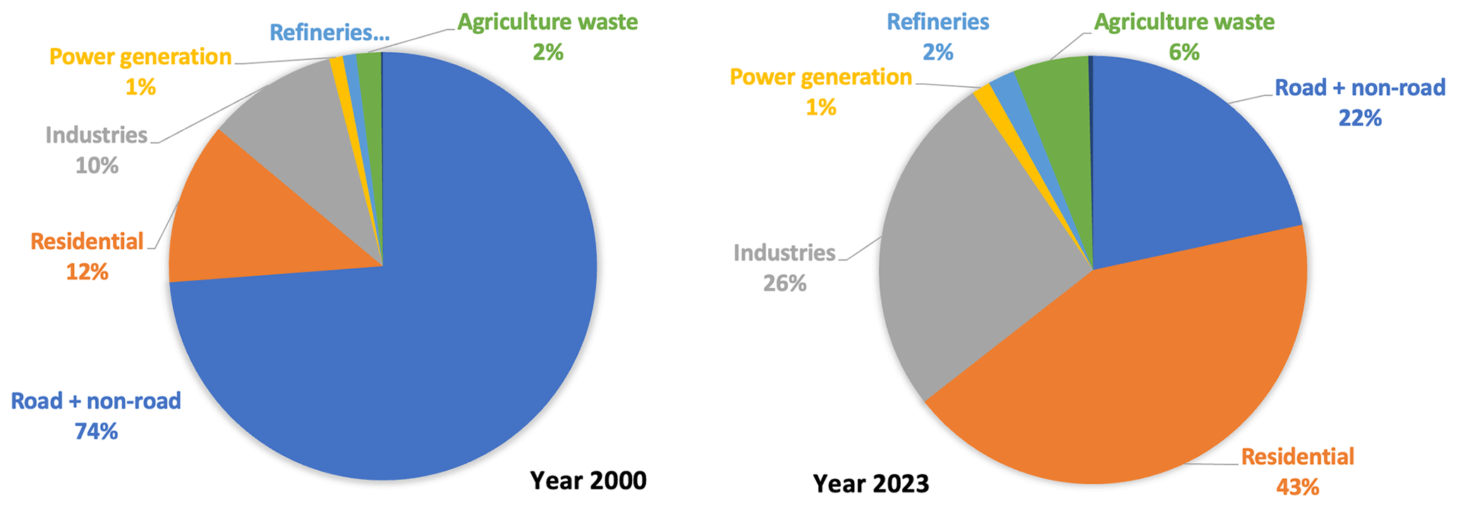
Figure 9 Contribution of several sectors to the CO emissions in western Europe in 2000 and 2023. The totals emitted for this region are 38.5 and 13.5 Tg yr⁻¹ in 2000 and 2023, respectively.

For CO, the decrease in the emissions is mostly due to the implementation of strict rules in all European countries on the emissions from transportation: these emissions from transportation change from 28 Tg CO yr⁻¹ in 2000 to 2.9 Tg CO yr⁻¹ in 2023, with the largest change during the 2000–2012 period. Such changes have significantly modified the contribution of each sector to the total CO emissions in western Europe, as shown in Fig. 9: while the emissions from transportation represented 74 % of the total emissions in 2000, they represent 21 % of the total in 2023. The highest contribution to the emissions in 2023 is from the residential (43 %) and industrial (26 %) sectors.

The decrease in NO_x emissions is also mostly due to a decrease in the emissions from transportation, as shown in Fig. S1, and to a lesser extent to the emissions from power generation: the contribution of the NO_x emissions from transportation decreased from 53 % in 2000 to 41 % in 2023, and the contribution of power generation decreased from 17 % to 11 % for the same period. At the same time, the contribution of industrial activities, which remained rather constant, increased from 12 % to 16 %.

NMVOC emissions also decreased significantly, as shown in Table 2, mostly during the 2000s and early 2010s. This is mostly due to the decrease in the emissions of transportation, but as the emissions from the solvents sector did not decrease, the NMVOC emissions decreased only by 3 % during the past decade.

SO₂ emissions from power plants, which were still rather important in 2000, have been strongly regulated and decreased from 2.5 to 0.8 Tg SO₂ yr⁻¹ in 2023. However, the emissions of SO₂ from industrial activities, the second largest contributor to SO₂ emissions, have decreased by about 30 % of the full period, which explains the decrease in the emissions reported in Table 1.

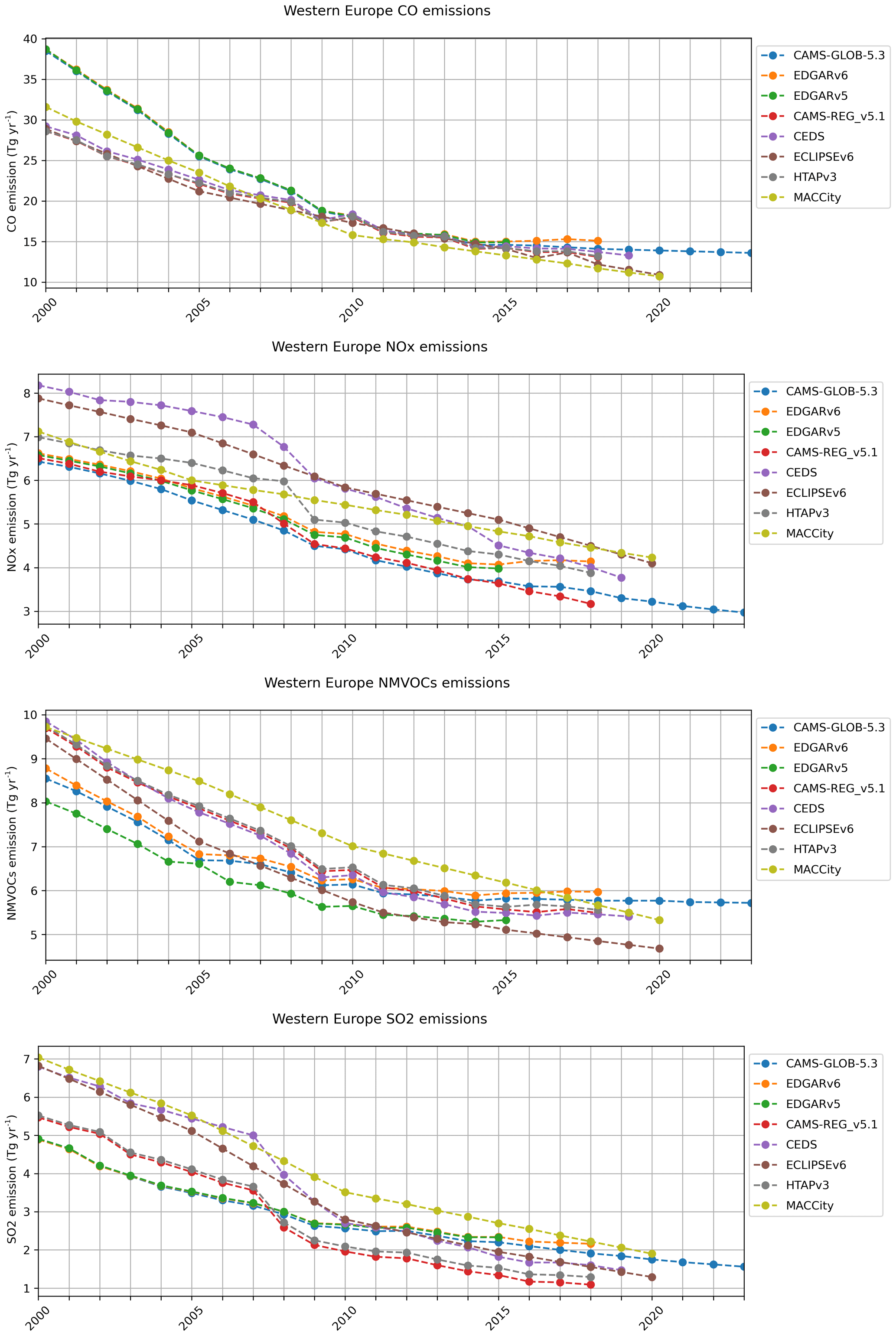
Figure 10 Comparisons of the CAMS-GLOB-ANT_v5.3 emissions for CO, NO_x, NMVOCs and SO₂ with other global datasets and the CAMS-REG_v5.1 inventory for western Europe.

Figure 10 shows a comparison of the CAMS-GLOB-ANT_v5.3 emissions with other inventories, i.e., the global inventories indicated at the beginning of Sect. 5, as well as with version 5.1 of the regional CAMS-REG dataset (Kuenen et al., 2022). For CO, all the inventories show similar values after 2009, except for MACCity and ECLIPSE, which show lower emissions after 2010: these two inventories are based on older scenarios after 2000–2005. For NO_x, the trends are similar among the inventories, with downward trends for the whole period. MACCity and ECLIPSE, based on scenarios, provide higher NO_x emissions in the most recent years. CAMS-GLOB-ANT and CAMS-REG show rather similar values: these two datasets use very different methodologies, CAMS-REG being based on values reported by countries to the European Monitoring and Evaluation Programme (EMEP; Wankmüller, 2019), while CAMS-GLOB-ANT is based on EDGARv5 and CEDS. For SO₂, the CAMS-GLOB-ANT emissions, which follow the EDGARv5 and the trends in the CEDS emissions, are higher than the regional emissions at the end of the period and slightly lower at the beginning of the period.

Rather similar patterns are seen in the change in the emissions of pollutants and greenhouse gases in central Europe (Table 3; Fig. S2), with decreases in somewhat lower magnitudes, related to smaller changes in transportation emissions. The emissions of BC and OC have increased during the first considered period, mostly due to an increase in residential combustion and to road transportation to a lesser extent.

Plots of the comparisons of the emissions for central Europe with global inventories and the regional CAMS-REG_v5.1 inventory are shown in Fig. S3. The results of the comparison are similar to the comparisons for western Europe: a larger spread of the values for the NMVOC emissions can be noticed which could be related to the use of different average emission factors for these compounds, which represents the emissions of a lumping of different species.

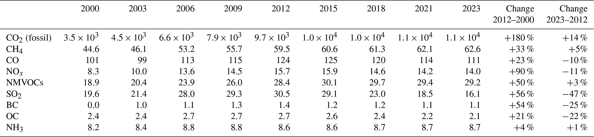
Table 4 Totals emitted in Tg yr⁻¹ and associated percentage changes for the USA. CO₂ (fossil) corresponds to the CO₂ species, excluding short cycle. The values for the NO_x emissions are given in Tg NO_x (as NO) yr⁻¹.

5.2 United States of America

Changes in the US emissions of several species for the same years, as considered in Table 1, are given in Table 4. The emissions of all species have decreased significantly, except for CH₄ and NH₃. The stability in the CH₄ emissions is related to constant oil and gas operations, as well as to livestock agriculture practices (fugitive and manure/enteric fermentation emissions in the EDGAR emissions). For NH₃, the constant increase is due to the use of fertilizers and livestock operations.

The changes in the emissions for the different sectors from 2000 to 2023 are shown in Fig. S4 for CO, NO_x, NMVOCs and SO₂. The large decrease in CO emissions is mostly due to the decrease in the emissions from transportation, with the implementation of national standards for tailpipe emissions, new fuel programs and improvement in vehicle technologies. These standards are described in detail on the website of the US Environmental Protection Agency (EPA; https://www.epa.gov/air-emissions-inventories; last access: April 2024). NO_x emissions decreased significantly until the early 2010s, but a slowdown in the emissions reduction has been seen since 2012, which is consistent with the study of Jiang et al. (2018) based on satellite and ground-based observations. This slowdown can be explained by a growing contribution of off-road and diesel vehicle transportation emissions, as well as industrial activities. The large decrease in SO₂ emissions is mostly due to the strict control in the emissions from power plants.

Comparisons were performed with the global datasets together with the officially reported emissions by the EPA. The air pollution emissions trend data from 1970 to 2021 provided by EPA at https://www.epa.gov/air-emissions-inventories/air-pollutant-emissions-trends-data (last access: April 2024) were used. Rather good agreement is seen for the CO and NO_x emissions in the USA, except for the EDGARv6 emissions of CO, which are significantly lower. This is due to the use of smaller emission factors for road transportation and lower small-scale combustion of biofuels in the EDGARv6 dataset.

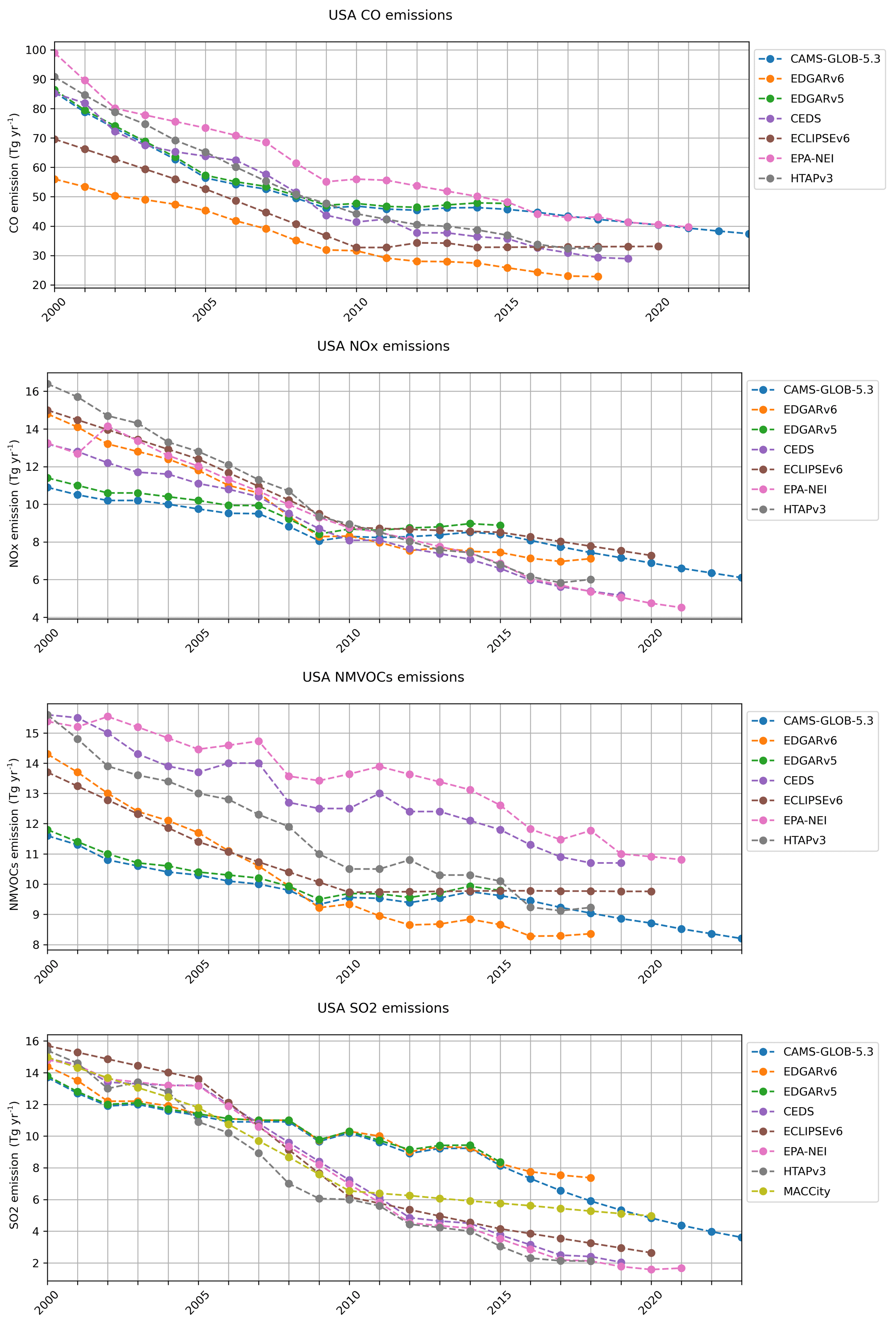
Figure 11 Comparisons of the CAMS-GLOB-ANT_v5.3 emissions for CO, NO_x, NMVOCs and SO₂ with other global datasets and the EPA inventory for the USA.

The differences shown in Fig. 11 between the inventories are larger for the NMVOC species, particularly in the early 2010s, with larger emissions from the EPA dataset and the lowest values in the old MACCity emissions and in EDGARv6. These differences are related to the road transportation sector and to a lesser extent to the solvents sector.

Table 5 Totals emitted in Tg yr⁻¹ and associated percentage changes for China. CO₂ (fossil) corresponds to the CO₂ species, excluding short cycle. The values for the NO_x emissions are given in Tg NO_x (as NO) yr⁻¹.

5.3 China

Table 5, which shows the changes in the emissions of several species for the same years as considered in the previous tables, reflects the measures taken as part of the Chinese Air Pollution Prevention and Control Action Plan established by the Chinese government in the early 2010s. From 2000 to 2012, the emissions of all species (except NH₃) increased by 20 % to 50 % for most pollutants, and even 90 % for NO_x. After 2012, only the emissions of CO₂ continued to increase, as well as the emissions of NMVOCs and NH₃ but with a low percentage.

The changes in the emissions for the different sectors from 2000 to 2023 are shown in Fig. S5 for CO, NO_x, NMVOCs and SO₂. The largest decreases after 2012 are for SO₂, for which the emissions from power generation and industrial processes decreased by 64 % and 47 %, respectively. NO_x emissions decreased as well, due to a 35 % and 9 % reduction in the emissions from power generation and industrial activities, respectively, and a minor reduction in the emissions from transportation. For CO, the main reductions from 2012 to 2023 are seen in the sectors of transportation (−24 %), residential (−20 %) and industrial activities (−11 %). The NMVOC emissions started to decrease slightly in 2015 as a result of a decrease in the emissions from transportation and from industrial processes. However, the emissions from solvents increased by 14 % between 2012 and 2023.

Comparisons were performed with the global datasets, as well as with two regional inventories for China: the Regional Emission inventory in Asia (REAS) version 3 published by Kurokawa and Ohara (2020) was used, downloaded from the REAS website (https://www.nies.go.jp/REAS/; last access: April 2024), as well as the Multi-resolution Emission Inventory model for Climate and air pollution research (MEIC) (http://meicmodel.org.cn; last access: April 2024; Li et al., 2017; Zheng et al., 2018). REAS and MEIC provide emissions for a large number of species (except for CH₄) for 1950–2015 (REASv3) and 2008–2017 (MEICv1.3), respectively.

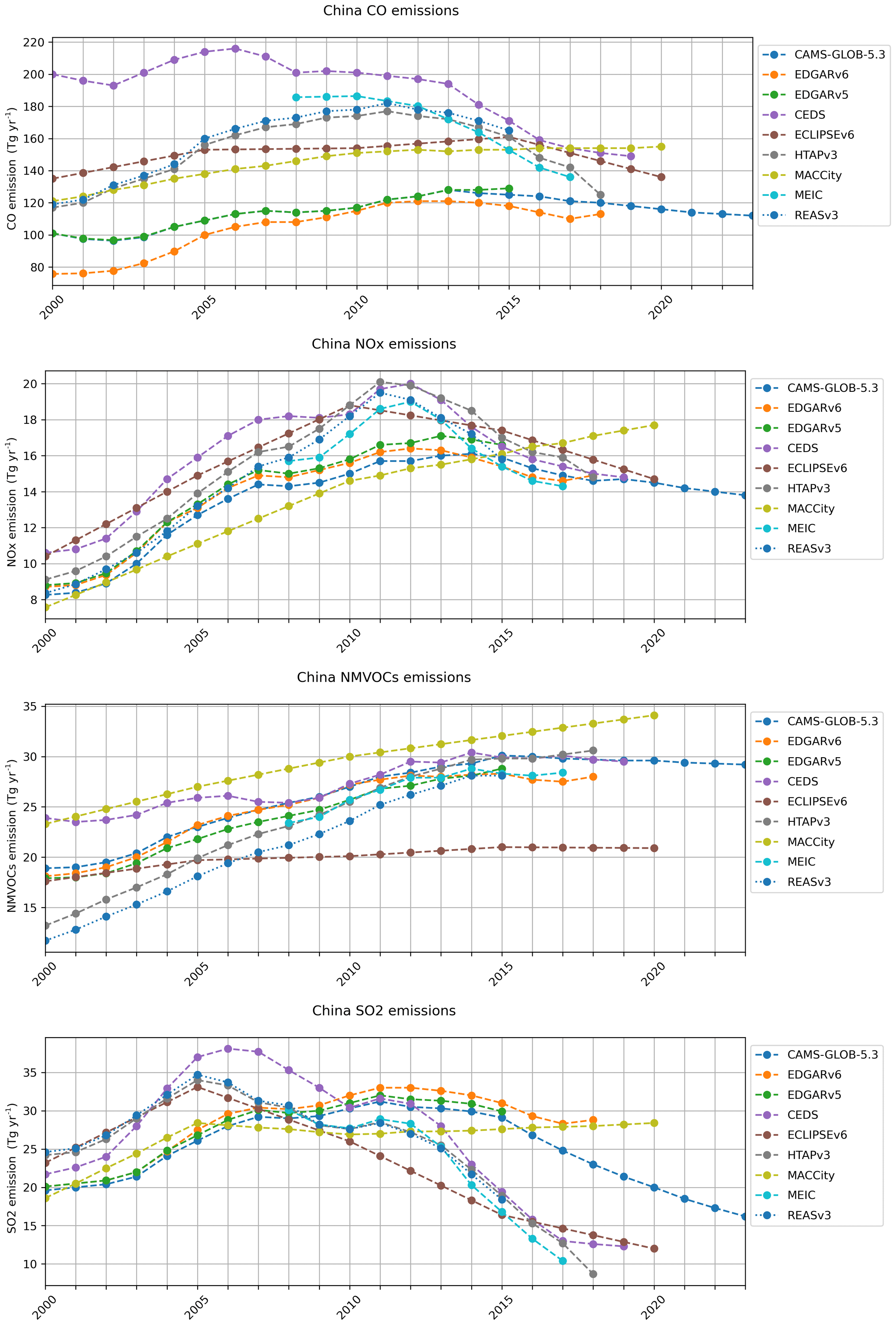
Figure 12 Comparisons of the CAMS-GLOB-ANT_v5.3 emissions for CO, NO_x, NMVOCs and SO₂ with other global datasets and two regional inventories for China.

Figure 12 shows the differences between these inventories for CO, NO_x, NMVOCs and SO₂. For CO, large differences exist at the beginning of the 2000s, but the total emissions for China are closer at the end of the period. The large differences are mostly due to different estimates of the emissions from transportation between the global inventories, more particularly CEDS and EDGAR. It should be noted that the two regional inventories, MEIC and REASv3, show CO emissions closer to the EDGAR emissions in the 2000s and closer to the CEDS emissions in the mid-2010s.

NO_x emissions show similar patterns among the global and regional datasets, except for MACCity, which was developed before the Chinese plans for emissions reductions (Zheng et al., 2018; Kurokawa and Ohara, 2020). In 2018, the NO_x emissions from all the inventories are within 15 % of each other. NMVOC emissions agree rather well in the 2010s, except for the old MACCity dataset and the ECLIPSEv6 inventory, which is also based on future scenarios. For SO₂, the agreement is rather good at the beginning of the 2000s, but the trends in the emission differ after 2013–2014, i.e., the EDGARv5 and EDGARv6 emissions show smaller trends than the other datasets. The emissions provided by CAMS-GLOB-ANT_v5.3 first follow the EDGAR emissions: as the recent trends are based on CEDS, the trend in the CAMS emissions is closer to the trend shown by the regional emissions. As a result, the values of the CAMS-GLOB-ANT SO₂ emission in 2015–2019 are between the EDGAR and the emissions provided by the other datasets.

Table 6 Totals emitted in Tg yr⁻¹ and associated percentage changes for India. CO₂ (fossil) corresponds to the CO₂ species, excluding short cycle. The values for the NO_x emissions are given in Tg NO_x (as NO) yr⁻¹.

5.4 India

Table 6 shows the changes in the emissions of several species for the same years as considered in the previous tables. This table shows the large increases in the emissions of all species in India from 2000 to 2012. After that period, some measures were taken to start reducing intense pollution events as part of the Indian National Clean Air Programme (Ganguly et al., 2020). Most emissions have continued to increase but at a slower rate than before 2012.

Figure S6 shows the changes in the CAMS-GLOB-ANT_v5.3 emissions of CO, NO_x, NMVOCs and SO₂ for the 2000–2023 period in India for the different sectors.

For all species, the emissions from the residential sector were almost constant during the considered period. The CO emissions peaked in 2015 and decreased afterwards as a result of the implementation of measures in the transportation and industrial sectors (Joshi et al., 2023). The NO_x emissions peaked as well in 2015 and stayed rather constant afterwards. This explains the slight increase in the emissions from 2012, driven by an increase in the emissions from transportation. Emissions of NMVOCs have continued to increase, mostly because of a constant increase of about 33 % of the emissions from solvents. The moderate increase after 2012 is related to a decrease in the emissions from traffic of about 16 % from 2015 to 2023.

SO₂ emissions are driven by the emissions related to power generation and industries, which more than doubled between 2000 and 2014, followed by rather constant emissions. For BC, emissions from industrial activities and the residential sector represent 40 % and 36 % of the emissions, respectively. The emissions from the industrial sector decreased by about 20 % from 2014 to 2023, which explains the slight decrease in the BC emissions during the 2012–2023 period.

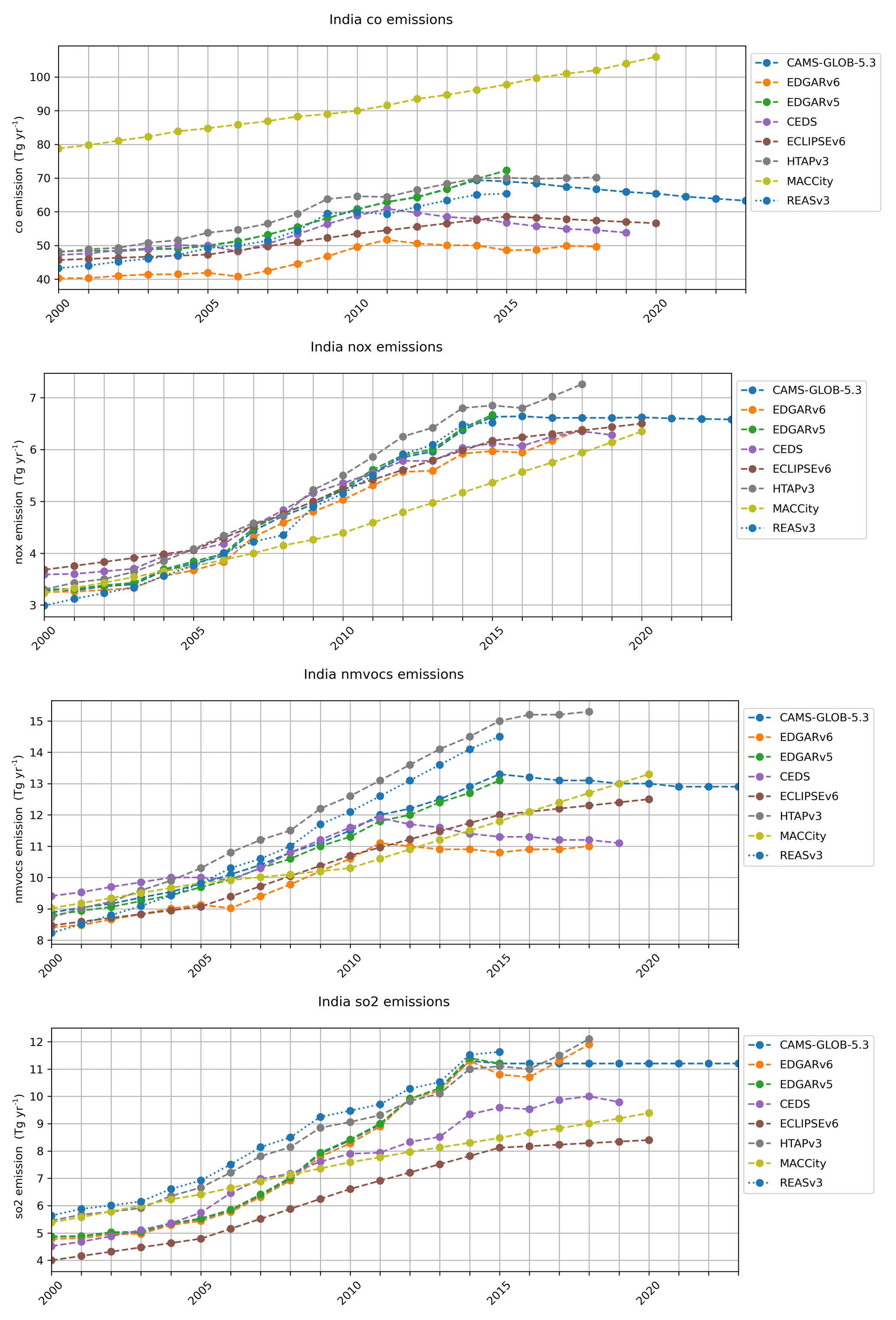
Figure 13 Comparisons of the CAMS-GLOB-ANT_v5.3 emissions for CO, NO_x, NMVOCs and SO₂ with other global datasets and two regional inventories for India.

Figure 13 shows a comparison of the emissions of CO, NO_x, NMVOCs and SO₂ with the global inventories mentioned in the previous sections and with the REASv3 regional inventory for Asia. The MACCity emissions, based on an old dataset (Granier et al., 2011) and the RCP8.5 scenario (Riahi et al., 2011), provides very different emissions than the other datasets. The other inventories are generally in good agreement, though the recent trends in the CAMS-GLOB-ANT emissions can differ significantly. For example, the NO_x emissions are rather constant after 2015, while they increase in the ECLIPSE dataset (based on a future scenario). For NMVOCs, the CAMS-GLOB-ANT emissions are rather stable after 2015, which is consistent with the HTAPv3 and EDGARv6; however, in 2015, CAMS-GLOB-ANT emissions are about 15 % lower than the HTAPv3 emissions and 20 % higher than the EDGARv6 emissions. For SO₂, the CAMS-GLOB-ANT emissions are in good agreement with the HTAPv3, EDGARv5 and EDGARv6 emissions, and significantly higher than the CEDS emissions. For all species, the CAMS-GLOB-ANT emissions are globally in agreement with the REAS regional inventory.

More evaluation of the CAMS-GLOB-ANT emissions are given in modeling studies that have used the CAMS models or other models such as the Multi-Scale Infrastructure for Chemistry Modeling (MUSICA; Tang et al., 2023) or the Community Earth System Model (CESM; Gaubert et al., 2021, 2023; Bouarar et al., 2021; Ortega et al., 2023).

6 Data availability

The gridded maps (CAMS-GLOB-ANT_v5.3) as monthly means data described in this paper can be accessed as Network Common Data Format (NetCDF) files at https://doi.org/10.24380/eets-qd81 (Soulie et al., 2023). They can also be accessed through the Emissions of atmospheric Compounds and Compilation of Ancillary Data (ECCAD) system at https://permalink.aeris-data.fr/CAMS-GLOB-ANT (last access: April 2024) and with a login account (https://eccad.aeris-data.fr/; last access: April 2024). For review purposes, ECCAD has set up an anonymous repository where subsets of CAMS-GLOB-ANT_v5.3 data can be accessed directly (https://doi.org/10.24380/eets-qd81; Soulie et al., 2023).

The CAMS-GLOB-ANT dataset is licensed under the Creative Commons Attribution 4.0 International license (CC BY 4.0). The summary of the license can be found here at https://creativecommons.org/licenses/by/4.0/legalcode (last access: April 2024).

7 Conclusions

This paper describes version 5 of CAMS-GLOB-ANT, a new inventory publicly available for global air quality as well as climate forecasts and reanalyses. The emission dataset is based on different datasets, i.e., the global inventories EDGAR and CEDS, as well as on temporal profiles from the CAMS-GLOB-TEMPO and ship emissions from the CAMS-GLOB-SHIP datasets. A dataset called CAMS-GLOB-AIR provides also three-dimensional emissions from aircraft exhaust. The CAMS-GLOB-ANT inventory was developed under the Copernicus Atmosphere Monitoring Service project (CAMS-81: global and regional emissions) as part of the European Union's Copernicus Earth Observation program.

CAMS-GLOB-ANT includes the emissions of 36 species, including the greenhouse gases CO₂ (excluding short cycle and short organic cycle), CH₄ and N₂O, as well as atmospheric pollutants (CO, NO_x, NMVOCs, SO₂, BC, OC and NH₃, plus 25 speciated volatile organic compounds). The spatial resolution of the gridded emissions is 0.1° × 0.1° in latitude and longitude, and the temporal resolution is monthly.

The paper discusses the changes in the emissions for the main greenhouse gases and air pollutants, with a focus on CO, NO_x, NMVOCs and SO₂. Comparisons are made with the other global inventories publicly available and with regional emission datasets available for Europe, the USA, China and India.

It should be noted that updated versions of the CAMS-GLOB-ANT dataset will be developed during the coming years. The current limitations of the inventory will be considered, such as the constant NMVOC speciation after 2012 (following the EDGAR VOC speciation), the inclusion of more up-to-date data for the extrapolations to the more recent years, the inclusion of the CONFORM adjustment factors for the COVID-19 lockdowns directly into the emission dataset and, when possible, the inclusion of regional information for the different species and sectors.