Deep Convective Microphysics Experiment (DCMEX) coordinated aircraft and ground observations: microphysics, aerosol, and dynamics during cumulonimbus development

Cloud feedbacks associated with deep convective anvils remain highly uncertain. In part, this uncertainty arises from a lack of understanding of how microphysical processes influence the cloud radiative effect. In particular, climate models have a poor representation of microphysics processes, thereby encouraging the collection and study of observation data to enable better representation of these processes in models. As such, the Deep Convective Microphysics Experiment (DCMEX) undertook an in situ aircraft and ground-based measurement campaign of New Mexico deep convective clouds during July–August 2022. The campaign coordinated a broad range of instrumentation measuring aerosol, cloud physics, radar, thermodynamics, dynamics, electric fields, and weather. This paper introduces the potential data user to DCMEX observational campaign characteristics, relevant instrument details, and references to more detailed instrument descriptions. Also included is information on the structure and important files in the dataset in order to aid the accessibility of the dataset to new users. Our overview of the campaign cases illustrates the complementary operational observations available and demonstrates the breadth of the campaign cases observed. During the campaign, a wide selection of environmental conditions occurred, ranging from dry, northerly air masses with low wind shear to moist, southerly air masses with high wind shear. This provided a wide range of different convective growth situations. Of 19 flight days, only 2 d lacked the formation of convective cloud. The dataset presented (https://doi.org/10.5285/B1211AD185E24B488D41DD98F957506C; Facility for Airborne Atmospheric Measurements et al., 2024) will help establish a new understanding of processes on the smallest cloud- and aerosol-particle scales and, once combined with operational satellite observations and modelling, can support efforts to reduce the uncertainty of anvil cloud radiative impacts on climate scales.

1 Introduction

Equilibrium climate sensitivity is a fundamental metric for assessing the risks of CO₂ emissions. Yet the plausible values of climate sensitivity have remained stubbornly uncertain for 40 years, with cloud feedbacks remaining a particularly uncertain component (Sherwood et al., 2020). The UK Natural Environment Research Council (NERC) has commissioned the CloudSense programme to focus on this problem (https://cloudsense.ac.uk/, last access: 2 May 2024). We present the observational campaign for one of the four CloudSense projects, the Deep Convective Microphysics Experiment (DCMEX).

Tropical high cloud, produced by deep convection, is an important cloud type when it comes to radiative effects and feedbacks (Bony et al., 2016; Hartmann et al., 2018; Gasparini et al., 2019). The IPCC Assessment Report 6 recently assessed there to be a negative feedback from tropical high cloud amount (e.g. cloud anvils) (Forster et al., 2021). This, however, came with low confidence, which arises, in part, from the lack of understanding of the microphysical response to warming. Gettelman and Sherwood (2016), for example, pointed out that there is significant spread in cloud feedbacks across different GCMs due to uncertainties in the representation of microphysical processes.

Quantitatively explaining the development of the ice particle types and size distributions in convective clouds remains a fundamental problem. There are many questions surrounding the initial production of cloud ice on ice-nucleating particles (INPs) (primary ice formation) (Kanji et al., 2017) and the development of high concentrations of cloud ice particles that dwarf the concentration of INPs (secondary ice production) (e.g. Cantrell and Heymsfield, 2005; Field et al., 2017). There are several candidate processes that might explain the unexpectedly high concentrations. The Hallett–Mossop (H-M) process of splinter production during riming (Hallett and Mossop, 1974) has been extensively investigated using aircraft measurements in cloud. Other, less-studied processes include droplet shattering (Lauber et al., 2018; Lawson et al., 2022) and collision fragmentation (Yano and Phillips, 2011). Challenges that will be addressed using the DCMEX dataset include determining which process or processes can explain the observed distribution of cloud ice particles. If preliminary analysis of observations in DCMEX supports previous results regarding the importance of the H-M process, another challenge will be to determine an improved parametrisation of the H-M process.

In July–August 2022, the DCMEX observation campaign was undertaken over the Magdalena Mountains, New Mexico. The aim was to carry out coordinated measurement of the aerosol, microphysics, and dynamics of deep convective cloud formation. The Magdalena Mountains near Socorro, New Mexico provide ideal laboratory-like conditions for this study. Isolated convective clouds reliably form and grow over the mountains as a result of orographic convection during the North American summer (Dye et al., 1989). Our campaign built on microphysics-only measurements taken at the very same location in 1987 using the National Center for Atmospheric Research (NCAR) King Air aircraft (Blyth and Latham, 1993; Blyth et al., 1997). Several important observations, which will guide analysis in DCMEX, arose from that early campaign:

• Primary ice particles, in concentrations consistent with the Cooper (1986) nucleation curve, were first observed when the in-cloud temperature reached about −10 °C. Improved instrumentation in DCMEX should allow us to better detect primary ice particles and relate them to concentrations of INPs. This is a key step, since INPs were not measured in the 1987 project.

• Clouds often contained supercooled raindrops that were observed prior to the formation of ice particles, despite the concentration of cloud drops being in excess of 700 cm⁻³.

• Clouds consisted of multiple thermals whose tops gradually ascended with time until eventually there was a transition to a thunderstorm from cumulus congestus with tops at about −15 °C (Raymond and Blyth, 1992). The sudden transition highlights a key feature for modelling electrification processes.

• There was evidence that the H-M process of splinter production during riming was responsible for the large concentration of ice particles. This result is consistent with subsequent research on the process. Improvements in cloud particle instrumentation, such as the ability to measure smaller particles and the reduction of ice-shattering artefacts, offer the opportunity to increase our understanding and confidence in the H-M process.

• Finally, an interesting observation was made regarding the cloud base. On the one occasion when the cloud base was much higher than usual due to lower humidity, the largest cloud droplets were too small to satisfy the criterion (d≥24 µm) for the operation of the H-M process (Mossop, 1978). A good understanding of such thresholds will enable more detailed parametrisations to be applied within models.

The DCMEX 2022 campaign described here has built upon the 1987 campaign not only through the use of state-of-the-art cloud physics instruments but also by coordinating observations of the whole aerosol–microphysics–dynamics–radiation system. This extensive dataset will be used to develop knowledge of microphysical processes and improve microphysical parametrisations in models. Then, using these new tools and foundational understanding, the stage is set to target deep insights into convective-cloud feedbacks that can help reduce uncertainty in equilibrium climate sensitivity.

A vast array of instruments were used for the campaign. The UK's BAe-146-301 atmospheric research aircraft made measurements of cloud microphysics, aerosol and dynamics in and around the clouds whilst dual-Doppler radars and automated digital cameras monitored the cloud growth from nearby. Aerosol measurements, including those of INPs, were collected on the aircraft and at the Langmuir Laboratory for Atmospheric Research on the summit of the Magdalena Mountain Range (33.98° N, 107.18° W). Within the DCMEX project, these data will be analysed in combination with satellite radiation products from the Geostationary Operational Environmental Satellite (GOES) R series and the Clouds and the Earth’s Radiant Energy System (CERES). Meanwhile, support of modelling activities will focus on the recently developed Cloud-AeroSol Interacting Microphysics (CASIM) module that can be used within the Met Office Unified Model (Miltenberger et al., 2018a, b; Hawker et al., 2021; Field et al., 2023). Altogether, the dataset will enable (1) the development and testing of the microphysics schemes applied in global climate models and (2) increased understanding of deep convective processes that impact the cloud radiative effect and feedbacks. These two components will support the overarching goal of DCMEX to reduce climate sensitivity uncertainty.

2 Flight and ground-based operations

In total, there were 19 flights over the course of the 24 d between 16 July and 8 August 2022. Every flight involved taking off from Albuquerque International Sunport between 15:00 and 16:15 UTC (09:00 to 10:15 a.m. local time, i.e. Mountain Daylight Time). Flight durations varied between approximately 3–4.5 h (Table 1). Each flight involved a profile ascent to 8–9 km above sea level (a.s.l., used for all altitudes given in this paper) followed by the deployment of a dropsonde in the vicinity of the Magdalena Mountains. Over the course of the rest of the flight, there was a mixture of cloud passes and aerosol runs, depending on the conditions. Aerosol runs were generally conducted first, partly to characterise the airmass that the clouds formed within and partly to allow for a rapid response to convective initiation once it started. Figure 1 shows the key waypoints used for the majority of runs during flights. In addition, a few runs were made around the San Mateo Mountains to the southwest when clouds were not present over the Magdalena Mountains. Figure 1 illustrates the flight stages described above as well as example cloud passes undertaken during the campaign.

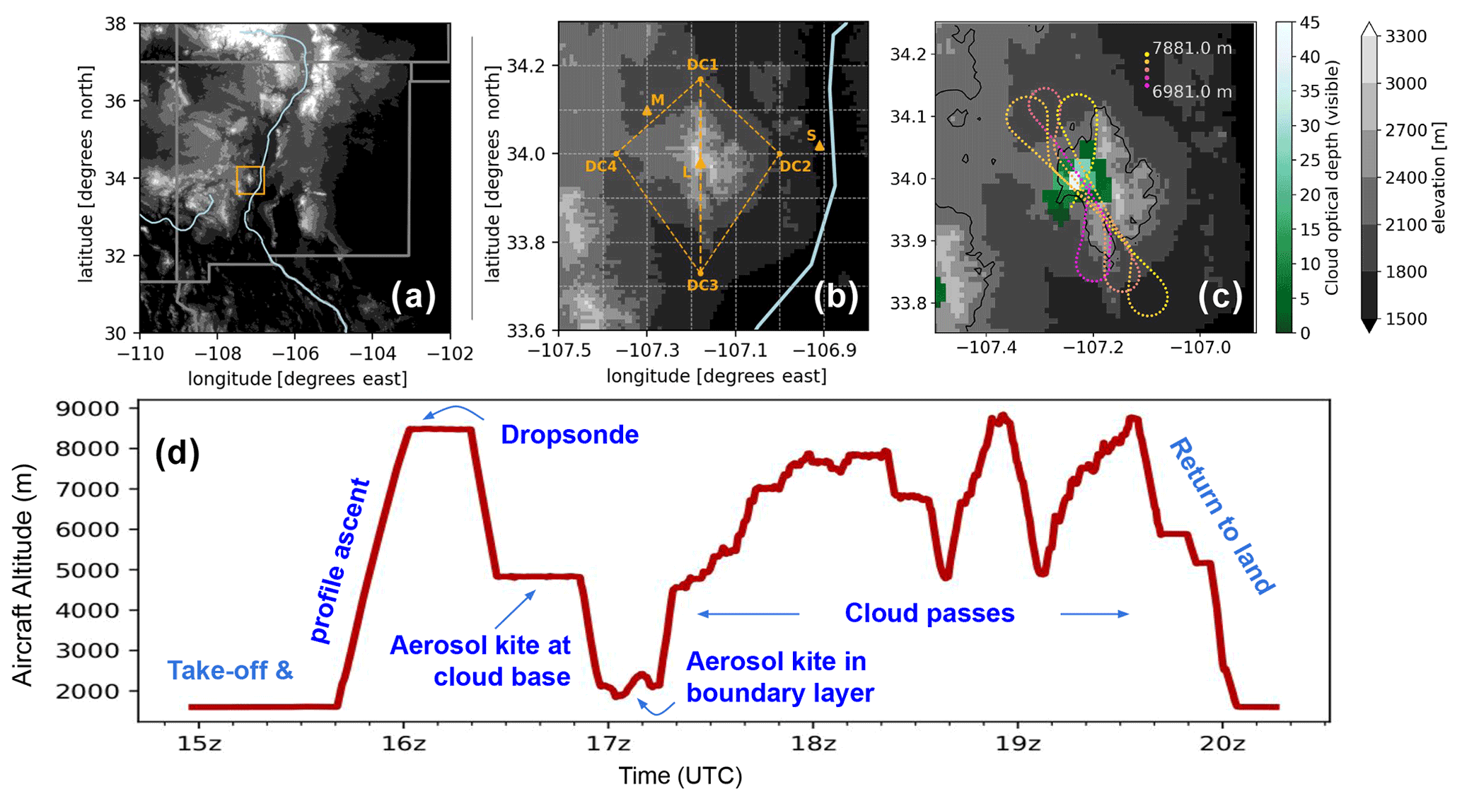
Figure 1 The main study region and representative flight paths. (a) The DCMEX study region (box) in the context of the terrain in New Mexico, USA. State borders are shown in grey. Rivers, including the Rio Grande in New Mexico, are shown in light blue. (b) Core flight coordinates and locations of instruments. Polygon DC1–DC4 shows the kite path that was used for aerosol runs, while line DC1–DC3 shows the nominal path for cloud passes, though there was substantial deviation from this. The letter L marks the Langmuir Laboratory, S marks Socorro Airport, and M marks Magdalena Airport. The airports hosted the radars and cameras and the laboratory hosted weather, aerosol, and electric-field instruments. (c) Flight track locations/altitudes between 17:45z and 18:15z on the 22 July flight. This is plotted over the GOES cloud optical depth observation at 18:02z. GOES data were downloaded using the goes2go Python package (Blaylock, 2023). The cloud optical depth field was corrected for parallax shift on a pixel-by-pixel basis using the GOES cloud top height product (Ayala et al., 2023); the result was then regridded to 0.1° regular grid for plotting (Finney, 2023). The black contour shows 2250 m terrain height. (d) Flight altitude and activities on 22 July. The 22 July flight provides a illustration of the general flight characteristics.

Basic details regarding the cloud and aerosol runs are provided in Table 1. In addition to the flights listed here, a UK test flight with a flight ID of c296 is included in the dataset. Aerosol runs around the base of the mountains took the form of a kite, with runs performed between waypoints designated DC1 (34.17° N, 107.18° W), DC2 (34.00° N, 107.00° W), DC3 (33.73° N, 107.18° W), and DC4 (34.00° N, 107.37° W) (Fig. 1). The kite was flown either clockwise or anti-clockwise, depending on the conditions, and was used to sample aerosols, including the INPs, dynamics, and thermodynamics within the boundary-layer inflow. As well as low-level, terrain-following runs, aerosol kite runs were also carried out close to cloud base height and at higher altitudes in relatively clean free-tropospheric air.

Cloud passes generally aimed to sample developing congestus clouds at various heights from close to cloud base up to about the −20 °C isotherm. Two approaches were used as deemed appropriate by the mission scientist: (1) the sampling of congestus turrets multiple times ∼200 m below cloud top as they grew over the course of the flight or (2) repeated sampling between −3 and −10 °C (the H-M zone). The first approach mainly targeted initial ice formation where it was known there was no influence from falling ice. The second approach focused on forming a time series of ice formation within the mixed-phase region, which is especially known for secondary ice formation. Secondary ice due to the H-M process could also be sampled in the first approach due to multiple thermals and the time taken to ascend to low temperatures. When sensible to do so, cloud passes followed the north–south line between DC1 and DC3 (Fig. 1), as this followed the mountain ridge and was broadly aligned parallel to the prevailing wind flow. As intense cumulonimbus clouds developed, it was not always possible to take this path, and alternatives were developed as required and based on the conditions at the time.

Table 1 Overview of flights and their sampling features. Asterisks mark runs that were terrain following. Many of the cloud runs comprise grouped individual cloud passes that are separated by less than 60 s. Only runs lasting longer than 5 s and with altitudes above 4 km are counted. Near-cloud temperatures for the lowest- and highest-altitude cloud passes were averaged from the 1 Hz measurements in the 15 s before entering cloud. The deiced temperature was used for temperatures $<=\mathrm{273}$ K and the non-deiced temperature for >273 K. If the preceding 15 s contained no data, then the post-cloud 15 s period was used if data were available.

* Excluded due to a highly varying altitude during long stratus cloud passes. n/a: not applicable.

To the east and northwest of the Magdalena Mountains are the Socorro and Magdalena airports, respectively. These were used as the locations for the radars and automated digital cameras. Together, these instruments provided a more comprehensive overall view of the cloud than the aircraft could provide alone, and they monitored the cloud continuously both before and after the aircraft was sampling. In addition to each instrument's unique perspective, the coincident measurements of different instruments will allow a more detailed description of cloud growth, e.g. through better-constrained estimates of turret ascent rates.

Whilst the aircraft measured boundary-layer aerosol in each flight, a static continuous measurement at the surface is a beneficial addition. Therefore, aerosol and INP samples were collected at Langmuir Laboratory for Atmospheric Research on top of the Magdalena Mountains. Automatic weather stations were also installed to provide continuous local surface weather. The Langmuir Laboratory has been extensively used for storm electrification measurements (Edens et al., 2019; Jensen et al., 2021), and it provided live electric-field measurements that were key, in combination with live radar, to avoiding the first lightning stroke as storms developed.

The above measurements complement those from weather stations, satellites, and sonde releases already in operation across New Mexico. In particular, the GOES and CERES satellite imagery will prove invaluable when relating microphysical processes to the radiative properties of the cumulonimbus anvils. Figure 2 illustrates the spatial and temporal relationships between instruments, and Tables S1–S3 in the Supplement list details of instrument operation across the campaign.

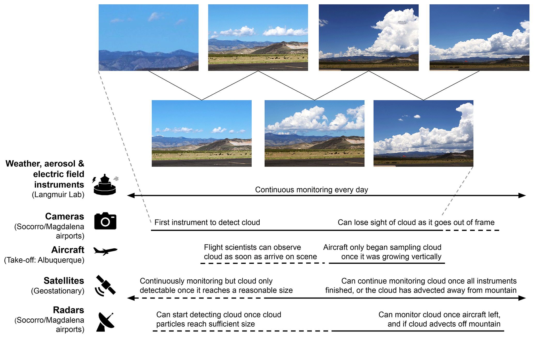
Figure 2 Indicative stages of cloud growth at which different instruments made observations and detected the cloud. Dashed lines indicate when the instruments were operational, and solid lines indicate representative periods when the instruments were able to detect the cloud. Tables S1–S3 provide details of instrument operation for each day of the campaign.

Flight days were mainly decided on the preceding day. Decisions were partly informed by national and local operational forecast tools, including the High Resolution Rapid Refresh forecast model produced by the National Oceanic and Atmospheric Administration of the USA. In addition, three bespoke high-resolution model forecasts were produced daily during the DCMEX campaign. The models used were the UK Met Office Unified Model (configurations: RA2m and RAL3) and the Weather Research and Forecasting model. These models were able to clearly simulate cumulonimbus development and, on the whole, provided robust forecasts in line with the ebb and flow of the convective activity during the campaign.

3 Instrumentation

Many different UK and US research teams came together to provide coordinated operation of instruments for this campaign. Below is a list of the key instruments operated to produce data to address DCMEX objectives. The data from these instruments are published to facilitate wider use of the dataset outside the DCMEX project.

3.1 FAAM BAe-146 aircraft

The Facility for Airborne Atmospheric Measurements (FAAM) BAe-146 aircraft is owned by UK Research and Innovation and NERC. It is managed through the National Centre for Atmospheric Science to provide an aircraft measurement platform for use by the UK atmospheric research community on campaigns throughout the world. A bespoke configuration of instruments, concentrating on measurements of dynamics, thermodynamics, aerosols, and cloud particles, was installed on the aircraft for DCMEX. Most aerosol instruments were installed in the cabin behind various inlets, while cloud spectrometer and imaging probes were installed on pylons under each wing. During sampling runs, the aircraft flies at a constant 200 kn (102.8 m s⁻¹) indicated air speed. Thus, true air speed increases with altitude (with a corresponding decrease in the spatial resolution of measurements).

All instruments in this dataset were time synchronised with the FAAM on-board time server. Two Meinberg LANTIME M600/GPS/PTP Stratum 1 time servers on board provide Precise Time Protocol (PTP) version 2 and Network Time Protocol (NTP) reference time signals to all PTP- and NTP-compatible systems connected to the aircraft network. They are updated to Institute of Electrical and Electronics Engineers (IEEE) standard 1588-2019, with one being configured as the grandmaster clock so that all PTP clients use the same server. The second M600 is there for redundancy and will switch from passive to grandmaster when required. All measurements should thus be synchronised to the same time stamp on a microsecond (for PTP) or millisecond (NTP) scale.

Figure 3 summarises the particle-size detection ranges of the aerosol and cloud instruments aboard the aircraft, along with their sampling rates. They cover the important sizes required for the research, spanning from the submicron to the millimetre and centimetre ranges. An overview of each instrument and its operation is provided in the following sections.

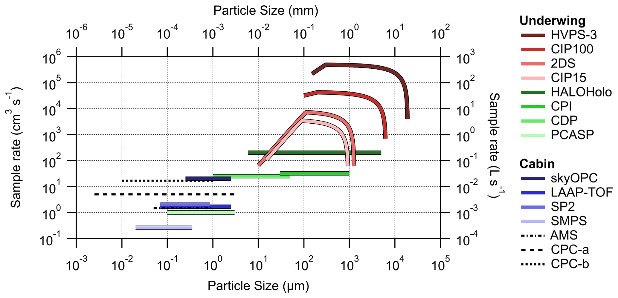
Figure 3 Nominal sampling rates of the various aerosol and cloud particle detectors operated on the FAAM aircraft during the DCMEX campaign, assuming an airspeed of 100 m s⁻¹. Condensation particle counter (CPC)-a is used for measuring aerosol number concentrations, and CPC-b is used for measuring cloud-residue number concentrations. For aerosol instruments, the dashed lines (including the aerosol mass spectrometer (AMS), CPC-a, and CPC-b) represent bulk aerosol measurements, and the solid lines represent size-resolved aerosol measurements. The SMPS (Scanning Mobility Particle Sizer) sample rate is the average sample rate over a full scan. The size dependence of the sampling rate for the optical array probes – HVPS-3 (High-Volume Precipitation Spectrometer 3), CIP100 (Cloud Imaging Probe with a resolution of 100 μm), 2D-S (Two-Dimensional (Stereo) probe), and CIP15 (Cloud Imaging Probe with a resolution of 15 μm) – is a result of (i) the post-processing, which rejects partially imaged particles, and (ii) the size dependence of the depth of field of the imaging systems (Knollenberg, 1970). The sample volumes assume that the particles are spherical and do not include the effects of dead time and coincidence, which vary with ambient concentration. The data shown assume an ambient pressure of 1000 mb.

3.1.1 Aerosol instruments

The aircraft was equipped with a series of instruments for online aerosol characterisation (i.e. for determining aerosol loadings, chemical composition, and size distributions) and the offline characterisation of INPs. The characteristics of aerosols ingested into the base of the cloud are of interest for interpreting the size distribution of cloud droplets at the cloud base and the distribution of primary ice particles (which form later). They also provide a signature of the air masses that influence the clouds, offering a potential link between the microphysical and synoptic scales. It is not only the low-level, boundary-layer aerosol particles that are of interest. There is the possibility of entraining INPs and cloud condensation nuclei (CCN) into the cloud at higher levels. Furthermore, aerosols at these higher levels may have been processed through previous clouds and left in detrained cloud layers or anvils before they re-enter the clouds of interest.

In this study, a Counterflow Virtual Impactor (CVI) inlet was used. The working principles of the CVI inlet are described in detail by Shingler et al. (2012). The CVI inlet with counterflow on is used to sample residue particles of cloud droplets. This only allows cloud droplets larger than the cut size to come into the inlet, and it obtains cloud residue particles by using dry and particle-free carrier air to evaporate the cloud water. During the campaign, the droplet cut size used was approximately 6.5 µm (aerodynamic diameter). The remaining cloud droplet residues can then be characterised by some online aerosol instruments behind the CVI inlet. Concentrations measured behind the CVI inlet have to be divided by an enhancement factor, which can be calculated based on the methods in Shingler et al. (2012). Furthermore, when the counterflow is off, the CVI inlet allows total air into the CVI inlet and can be used to sample ambient aerosols out of the cloud.

The principles and operation of the main aerosol instrumentation are listed below:

• Aerosol mass spectrometer (AMS). A compact time-of-flight aerosol mass spectrometer (C-TOF-AMS), manufactured by Aerodyne Research Inc., was employed to measure the chemical composition of non-refractory submicron aerosols (i.e. organic aerosol (OA), sulfate, nitrate, and ammonium), enabling chemical characterisation across a spectrum of ion mass-to-charge ($m/z$) ratios from 10 to 500 (Drewnick et al., 2005). Previous aircraft work has provided a detailed description of the AMS, including calibration and correction factors (e.g. Morgan et al., 2010). Briefly, the aerodynamic lens inlet system of the AMS focuses the particles into a narrow beam which passes through a particle-sizing chamber that is gradually evacuated to lower pressures. The strong vacuum in the chamber removes the majority of gases. Subsequently, the particles undergo flash vaporisation and ionisation steps. The fragment ions are then examined with a time-of-flight mass spectrometer (TOF-MS). The transmission of the particle beam to the TOF-MS is controlled by a “chopper”. When open, this determines the mass spectrum of the ensemble of particles, and the background mass spectrum is measured. When the chopper is placed in a “chopped” position, the P-TOF (particle time-of-flight) mode is used to record averaged mass size distribution data for the ensemble of particles. In this study, we employed an improved particle size measurement module, the efficient particle time-of-flight (e-PTOF) module, which has a better signal-to-noise ratio and an ∼50 % particle throughput. AMS calibration involved the utilisation of monodisperse particles of ammonium nitrate and ammonium sulfate. The AMS data underwent processing through the SQUIRREL (SeQUential Igor data RetRiEvaL, v. 1.65C) TOF-AMS software package (CIRES, 2024). To achieve better accuracy, we employed an algorithm introduced by Middlebrook et al. (2012) to correct data with a time- and composition-dependent collection efficiency.

• Condensation particle counter (CPC). A primary condensation particle counter (CPC) instrument was operated by FAAM and is referred to as “CPC-a” in Fig. 3. CPC-a is a water-based CPC (TSI model 3786) which is modified for low-pressure operation behind a constant-pressure inlet and measures over the size range 2.5 nm–3 µm. Ambient aerosols are sampled through a modified Rosemount Aerospace Inc. type 102 Total Temperature Housing. Due to losses associated with the in-cabin tubing, the minimum aerosol size (D50) is estimated to be 5.75 nm (Williams and Trembath, 2021). A second CPC instrument was operated to sample cloud residues downstream of a CVI inlet and is referred to as “CPC-b” in Fig. 3. CPC-b is a butanol-based CPC (TSI model 3010) that detects particles in the size range of 10 nm–1 µm. In principle, particles can grow into larger droplets in the CPC through the condensation of a supersaturated vapor (water or butanol) (Mordas et al., 2008). These droplets are then counted by a laser-diode optical detector.

• Passive Cavity Aerosol Spectrometer Probe (PCASP). A PCASP with SPP-200 electronics was operated in a wing-mounted canister. This instrument provides aggregated 5 Hz particle numbers in 30 size bins across a nominal diameter range of 0.1–3 µm. The smallest bin is discarded due to an undefined lower boundary, and bins are merged at the gain-stage crossover points as described by Ryder et al. (2013). Particles are binned according to the strength of the photovoltage generated by the HeNe laser light scattered by each particle. Laboratory calibrations both before and after the campaign are used to convert photovoltages into scattering cross-sections for each bin (Rosenberg et al., 2012). These calibrations are provided in separate files alongside the data files to be applied by the data user. With knowledge of the aerosols being sampled (that is, the particle shape and complex refractive index), the scattering cross-sections can be converted into particle diameters. This information must be determined through other means and applied by the users to obtain calibrated particle sizes and thus size distributions and any required derived parameters. The volumetric flow rate, which is used to calculate particle concentrations, was calibrated in the laboratory using either a Gilibrator 2 (Sensidyne, LP) low-flow wet cell or, more recently, a Gilibrator 3 dry-cell calibrator.

• Scanning Mobility Particle Sizer (SMPS). The SMPS (Grimm and Eatough, 2009) was utilised, along with the PCASP described above, to determine aerosol number size distributions. The SMPS collected samples from the same inlet as the AMS and assessed distributions of dry particle mobility diameter. Diameters were categorised into 40 logarithmically spaced bins within the range of 20 to 350 nm. To achieve this, a low-pressure, water-based condensation particle counter (WCPC model 3786-LP) was linked to a TSI 3081 differential mobility analyser. The SMPS scans through a voltage range and is able to produce the full size distribution of aerosol particles (20–350 nm) approximately once per minute. Given the time resolution, SMPS data are only available in straight and level runs and without rapid aerosol concentration changes. The SMPS data can be inverted using the inversion algorithms developed by Zhou (2001).

• Single Particle Soot Photometer (SP2). The refractory black carbon (hereafter referred to as BC) was characterised using an SP2 (Droplet Measurement Technologies, Boulder, CO, USA). The instrument setup, operation, and data interpretation procedures can be found elsewhere (McMeeking et al., 2010; Liu et al., 2010). The SP2 detects particles with an equivalent spherical diameter in the range of 70–850 nm. It can determine the BC mass within those particles and hence the BC mixing state. Two detectors capture the signal and identify the absorbing particle. The SP2 incandescence signal is proportional to the mass of refractory BC present in the particle, regardless of mixing state. The SP2 incandescence signal was calibrated using Aquadag black-carbon particle standards (Aqueous Deflocculated Acheson Graphite, manufactured by Acheson Inc., USA), including the use of the correction factor (0.75) recommended by Laborde et al. (2012). The mass can be then converted to a spherical-equivalent BC core diameter with an assumed BC density of 1.8 g cm⁻³.

• Teflon and polycarbonate filters. Aerosol for offline INP and compositional analysis was collected in parallel onto a pair of filters – polycarbonate track-etched membranes with a 0.4 µm pore diameter (Whatman Nuclepore 10417112) and polytetrafluoroethylene (PTFE) membranes with a 1.2 µm effective pore diameter (Sartorius type 11806) – from air sampled by the dual aircraft inlet. Sampling runs typically lasted 10–20 min and sampled volumes of air ranged between 87–987 L, depending on altitude, filter pore size, and filter support type, as calculated using air flow rates for each channel determined using an in-line flowmeter and data logger. A full characterisation of this system is given in Sanchez-Marroquin et al. (2019), and examples of its previous use for sampling INPs are given in Price et al. (2018) and Sanchez-Marroquin et al. (2021). Polycarbonate filters were divided and used for offline scanning electron microscopy (SEM) analysis and INP analysis, while PTFE filters were used for INP analysis only. Blank filters were taken on each flight to establish the limit of detection for INP concentrations: a pair of filters (a polycarbonate and a PTFE filter) were prepared and loaded into the sampling system as normal but only exposed to ambient air for around 1 s. INP analysis by droplet freezing assays (DFAs) combined with total air flow were used to determine INP concentrations per litre of air for each sampling run. A temporary laboratory for DFAs and clean handling of filters was established in Albuquerque, which allowed the PTFE filters to be analysed for INPs within 24–48 h of collection. The polycarbonate filters were stored in airtight filter cassettes, transported back to University of Leeds, and stored at −20 °C for DFA and SEM analysis. The hydrophobicity of PTFE filters enables the use of the “drop-on” DFA technique, where droplets of pure water are placed directly on the exposed filter, which is placed on a cooling stage (Price et al., 2018). Polycarbonate filters were analysed for INPs using the “wash-off” method, where the filter is placed in pure water to create a suspension that is subsequently pipetted onto a clean substrate mounted on a cooling stage (Whale et al., 2015). Using the drop-on DFA technique with PTFE filters enabled higher-sensitivity sampling of INPs (0.01–10 L⁻¹) compared to the wash-off method (1–100 L⁻¹), as the particles on the filter are not diluted by placing them in a suspension. Therefore, in combination with the higher air flow rates due to the larger pore size used, the “warmer” end of the INP spectrum for a single sampling run is captured by the analysis of PTFE filters, while the “colder” end is captured via the polycarbonate filters. A polycarbonate and PTFE filter pair was obtained for almost all aerosol run heights listed in Table 1. The only exceptions were that PTFE filters were collected from both inlets at each height on 19 and 20 July (i.e. there were no polycarbonate filters on those days) to ensure that both filter channels were providing equivalent samples. Selected filters were analysed by SEM (Tescan VEGA3 XM fitted with an X-max 150 silicon drift detector (SDD) energy-dispersive X-ray spectroscopy (EDS) detector) at the University of Leeds to determine the morphological and elemental composition of particles above 0.3 µm collected on the polycarbonate filters. This method, outlined in Sanchez-Marroquin et al. (2019), served to characterise the size distribution, surface area, and size-resolved composition of the collected aerosol using automated particle scanning. Classification software (Aztec 3.3, Oxford Instruments) enabled thousands of particles to be individually scanned on each filter and automatically classified into compositional classes such as mineral dust, carbonaceous particles, and sulfate-rich particles.

During campaign flights, it was necessary to determine if the upcoming run was a cloud run in order to set the appropriate operation of the CVI inlet. The cockpit crew would announce cloud runs prior to entering cloud, based on line of sight. For these in-cloud runs, cloud residues were sampled downstream of a CVI inlet with counterflow on. Cloud-residue number concentrations were measured with a butanol-based 3010 CPC operated by the University of Manchester (CPC-b in Fig. 3). Cloud-residue number size distributions were measured by the GRIMM sky optical particle counter (skyOPC). The chemical composition and mixing state of cloud residue can be analysed by the AMS and SP2. When the aircraft was flying out of clouds, the onboard instruments, including the butanol-based CPC, sampled ambient air via the CVI inlet with the counterflow off. Onboard aerosol instruments, including the AMS, SP2, and SMPS, sampled ambient air via stainless steel tubing from a modified Rosemount inlet, which has sampling efficiencies close to unity for submicron particles (Trembath, 2013).

Combined, the instrumentation described above characterises the chemical composition and size distributions of aerosols. In addition, the potential for primary cloud-ice formation can be established through INP measurements.

3.1.2 Cloud physics instruments

The purpose of making aircraft cloud physics measurements in DCMEX was to provide information regarding the temporal and spatial distribution of cloud particles as the clouds developed. The instruments together provide coverage of the full range of cloud particle sizes and properties, including the quantification of concentrations and ice mass as a function of ice crystal habit. In addition, they enable the examination of fine morphological details to probe primary and secondary ice production (SIP) processes. Specifically, the data will be used to determine the properties of the primary and secondary ice particles as well as where precipitation particles first form and how they develop. A thorough review, including the instruments used here, was carried out by Baumgardner et al. (2017). The instruments used were as follows:

• Two-Dimensional (Stereo) probe (2D-S). The 2D-S instrument, manufactured by Stratton Park Engineering Company Inc. (SPEC), is the key cloud instrument for determining ice particle concentrations as a function of size and habit. It consists of two high-speed 128-photodiode linear array channels (orthogonal to each other and the direction of flight) and electronics to produce shadowgraph 2D stereo images of particles covering the nominal size range 10–1280 µm with a resolution of 10 µm (Lawson et al., 2006). Images can be captured at rates of up to 74 frames per second, depending on available data transmission rates. The sample volume of the instrument is approximately 16 L at an airspeed of 100 m s⁻¹. The instrument was also fitted with Korolev anti-shatter tips (Korolev et al., 2011; Lawson, 2011) to minimise particle-shattering artefacts. Analysis of 2D-S particle inter-arrival time histograms is used to identify and remove potential shattered particles (Field et al., 2006). Discrimination between spherical and irregular particles is achieved for particles typically greater than ∼50–100 µm in size using a circularity criterion (Crosier et al., 2011; Lloyd et al., 2020). The particle shape categories generated include low irregular (LI, with a defined shape factor between 1 and 1.2), indicating liquid droplets or newly frozen liquid droplets that maintain a near-spherical shape; medium irregular (MI; shape factor between 1.2 and 1.4) for increasingly irregular particles, likely indicative of ice; and high irregular (HI; shape factor >1.4), indicating ice particles. Particles comprising fewer pixels than a set threshold number (e.g. 20 pixels) are assigned to an “unclassified” shape category. The high sampling rate and resolution of the 2D-S allows the possible identification of regions where ice crystals are at their embryonic stage of formation and SIP mechanisms may be occurring (Lawson et al., 2006). However, in high cloud-particle concentration environments, some particles may not be recorded due to the probe's electronics being busy processing previous particles. These periods of probe “deadtime” are recorded for the correction of total particle concentrations (due to missed particles).

• Cloud Particle Imager (CPI). The CPI (SPEC Inc.) used was version 2.5, which uses a 1024×1024 pixel CMOS camera and data acquisition system capable of recording digital images of cloud particles with 8-bit greyscale (256 levels) at a pixel resolution of 2.3 µm and a maximum frame rate of 400 frames per second. The instrument was fitted with Korolev anti-shatter tips similar to the 2D-S. The CPI measures the size and shape of cloud particles with high resolution and enables an estimate of the relative concentration of water drops and ice particles in cloud. With appropriate depth-of-field corrections (e.g. Connolly et al., 2007), it is able to produce size distributions of particles greater than approximately 8 µm. Whilst the sample volume of the CPI is significantly smaller than for the 2D-S (approximately 0.37 L at 100 m s⁻¹ airspeed), it is particularly suited to providing high-resolution images for determining shapes and habits of ice crystals, which is an aid to understanding the growth history and potential origins of these particles (including the identification of potential SIP mechanisms (Korolev and Leisner, 2020; Korolev et al., 2022)).

• High Volume Precipitation Spectrometer (HVPS-3). The SPEC Inc. HVPS-3 (e.g. Lawson et al., 1998) uses a 128-photodiode array and electronics similar to the 2D-S probe. However, its optics are configured to provide images at 150 µm pixel resolution, giving it a nominal size range of 150–19 200 µm. This enables particles as large as 1.92 cm to be imaged, depending on the analysis technique employed. The presence of even larger particles can often be detected by observing the particle size in the direction of flight. The HVPS-3 has a typical sample volume of 310 L at an airspeed of 100 m s⁻¹ and is used in this study to identify low concentrations of graupel and large precipitation particles. Data processing is similar to that of the 2D-S, and further information can be found in the SPEC Inc. HVPS software manual (2010 and updates) and McFarquhar et al. (2017).

• Cloud Droplet Probe (CDP). The Droplet Measurement Technologies (DMT) CDP-2 (Lance et al., 2010) was flown on the same underwing canister containing the BCP-D (Backscatter Cloud Probe with Depolarisation). The CDP is an open-path instrument that measures the forward-scattered light (over subtended solid angles of 1.7–14°) from the 0.658 µm incident laser beam. Particles are assigned to 1 of 30 size bins over the nominal size range 2–50 µm. Size calibration was carried out pre-flight with 10 different-size glass beads with certified diameters and uncertainty (Rosenberg et al., 2012). Instrument windows were cleaned before each flight, and the optical alignment was found to be stable, resulting in minimal changes to the calibration throughout the campaign. A campaign master calibration was obtained by taking the average of each calibration size weighted by the uncertainty; note that data with a z-score greater than 5 were considered poor and discarded. The campaign calibration was applied to all flight data. The sample area was measured at 0.262 mm² with a droplet gun during manufacturer servicing in 2021. The CDP is sensitive to large dust aerosols as well as cloud droplets. Normally, conversion from the scattering cross-section is done using the refractive index of water, 1.33+0i, but other refractive indices may be applied for out-of-cloud measurements when appropriate. To obtain the highest possible spatial resolution, the CDP was operated at 25 Hz.

• Cloud Imaging Probes (CIPs) with resolutions of 15 μm (CIP15) and 100 μm (CIP100). Two DMT CIPs with differing resolutions were flown. Both probes use the same 64-pixel photodiode array, giving a size range of 15–930 and 100–6200 µm, respectively (the end pixels are used for edge detection, not particle sizing). Both CIPs produce 2-bit greyscale images, which allow for more accurate small-particle reconstruction (O'Shea et al., 2019, 2021). Anti-shatter tips were used on both probes.

• Nevzorov hot-wire probe. This probe, manufactured by Sky Physics Technology Inc., has sensors to measure the bulk liquid-water content (LWC) and the total condensed-water content (liquid plus ice) in cloud (Korolev et al., 1998). The vane used, which self-aligns to the airflow, consists of two coiled wires of 2 and 3 mm diameter for liquid-water content measurement and an 8 mm deep cup total-water sensor (Korolev et al., 2013). All elements were operated at 120 °C, and data were recorded at 64 Hz. Initial processing of the data is performed and archived with FAAM data. Additional processing has been undertaken by the UK Met Office following the technique described in Abel et al. (2014). Both sets of processed data are published in this dataset. In the Met-Office-processed data, cloud LWC and the ice water content are derived from the baseline-corrected measurements using the following assumptions: (i) the collection efficiencies of hydrometeors are assumed to be 1; (ii) the liquid-water sensors have been shown to measure a fraction of the ice water content in pure ice clouds, which is typically <15 % (Korolev et al., 1998) (it is assumed to be 11 % for the DCMEX data); and (iii) the difference between the total-water and liquid-water measurements is due to ice particles, although there could be contributions from drizzle and/or raindrops. Processed data are available at 1 and 64 Hz temporal resolution.

• SEA WCM-2000 hot-wire probe. This probe, described by Steen et al. (2016), has three sensing elements; liquid-water content is measured with two wire elements of diameters 2.11 and 0.53 mm, while the total condensed-water content is measured with a concave half-pipe, also of diameter 2.11 mm. Another element, oriented parallel to the airflow and free of incident water, is used to monitor changes in radiant cooling and so to compensate for variations in the ambient atmospheric conditions. All elements are operated at 120 °C, and the sample rate is set to 10 Hz. The measurements from this instrument were substantially lower than those of other instruments measuring liquid-water content. The reason is unknown, and the data are not used by the DCMEX project team.

3.1.3 Wind, temperature, humidity, and imagery instruments

A number of other instruments provide details of the dynamics and thermodynamics of the environment. Cameras mounted on the aircraft provide an additional perspective.

• Aircraft-Integrated Meteorological Measurement System (AIMMS-20) and other wind measurements. This instrument is manufactured by Aventech Research Inc. and was mounted in a canister under the port wing. As well as meteorological data, the AIMMS-20 measures 3D winds with a five-port probe positioned on a 0.425 m long boom. The probe tip can be heated if required to inhibit ice accumulation, and any water in the pressure lines can be purged with a low-pressure pneumatic system on demand. Wind data are recorded at 20 Hz with an uncertainty of 0.5 m s⁻¹ (Aventech Research Inc., 2024). 3D winds are also derived from the five-hole pressure measurement system in the aircraft radome. When the aircraft penetrates supercooled cloud, ice often forms on the radome, which invalidates the derived wind measurements. A small heater reduces the icing and also allows recovery from icing events. Further details are available in Petersen and Renfrew (2009) and Brown et al. (1983).

• Airborne Vertical Atmospheric Profiling System (AVAPS) and the manual dropsonde tube. The FAAM BAe-146 is outfitted with an AVAPS (UCAR/NCAR, 1993; Hock and Franklin, 1999). Vaisala RD41 dropsondes (Vömel et al., 2021) were used throughout the campaign to obtain vertical meteorological profiles above the ground site prior to in situ aerosol and cloud measurement runs. Before each launch, the thin-film capacitor relative humidity sensors were conditioned using the built-in AVAPS function. This provided a zero reference for the measurement (Jensen et al., 2016), resulting in an uncertainty of 2 % relative humidity.

• Aircraft-mounted video camera systems. The aircraft has four cameras operated as standard pointing in the forward, back, up, and down directions (relative to the airframe). The field of view of the camera lenses is 30° horizontal and 23° vertical.

• Humidity probes. Three types of hygrometers were used (Price, 2022): the General Eastern 1011B and the Buck CR2 (chilled mirror hygrometers) and the Water Vapor Sensing System (WVSS-II) from SpectraSensors. A calibrated volume mixing ratio measurement is determined using the Buck CR2 and WVSS-II in combination. This setup has a response time of around 2 s. The General Eastern hygrometer acts as a backup instrument.

• Temperature probes. Air temperature was measured with deiced and non-deiced internal sensors within two Rosemount model 102 housings (Price, 2022). These housings have similar inlets which draw flow across the sensing elements. They are designed to minimise water and particle ingress as well as to minimise the interaction of the air with the walls of the inlet. As far as possible, the housings bring the air to rest relative to the aircraft. The probes used were the 17005E (fast loom probe, non-deiced) and 20472E (plate probe, deiced).

• Total water probe. The total water probe is described by Nicholls et al. (1990) and Abel et al. (2014). In cloud-free air, the instrument measures the water vapour content with a Lyman-alpha hygrometer. During cloud penetrations, liquid and ice particles are evaporated by heating and mechanical break-up within the inlet upstream of the hygrometer. This provides a direct measurement of the total water content (vapour plus condensate). For DCMEX, the instrument was calibrated against the WVSS-II measurement in the cloud-free sections of each flight. The data were recorded and are available at 256 Hz.

3.2 Langmuir Laboratory

The Langmuir Laboratory for Atmospheric Research is located near to the summit of South Baldy Peak in the Magdalena Mountain Range, the location of the DCMEX study region (Fig. 1). The laboratory comprises a main building complex and separate underground (lightning-protected) laboratory bunkers or “kivas” located at the top of South Baldy Peak. Kiva-2 was instrumented with a set of aerosol, weather, and electric-field instruments which provided data during the field campaign.

Langmuir data from the aerosol spectrometer, a GRIMM OPC model 1.109, have been published. This instrument was installed at the Langmuir Kiva-2 laboratory located on South Baldy Peak at 3287 m a.s.l. It provides continuous aerosol size distribution measurements for particles from 0.25 to 32 µm in 32 size channels. The instrument was connected to a 4 m tall stainless-steel sample pipe mounted to the Kiva-2 rooftop (Fig. 4).

Meteorological station data from the site have also been published. One station, a Vaisala WTX536, was installed at the Kiva-2 laboratory. It was placed on the aerosol sampling mast to provide collocated wind speed, direction, temperature, relative-humidity, pressure, rainfall rate, and hail rate data. A second meteorological station, a Gill MaxiMet GMX600 Met Station (Fig. 4), was installed at the Langmuir Laboratory next to the Digitel aerosol filter sampler (described in Sect. 4) to provide measurements of wind speed, direction, temperature, humidity, pressure, and precipitation rate.

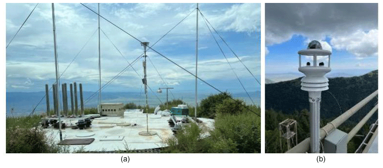
Figure 4 Photographs of aerosol detectors and automatic weather station locations on the Magdalena Mountains during the DCMEX campaign. (a) Kiva-2 Laboratory rooftop (South Baldy Peak), which includes a centrally mounted University of Manchester aerosol inlet with a Sigma-2 inlet and a Vaisala WXT536 meteorology station. (b) Gill MaxiMet GMX600 meteorology station (University of Manchester) mounted on the Langmuir Laboratory rooftop railing.

3.3 Doppler radars

Two dual-polarisation Doppler weather radars were deployed during the field campaign to obtain targeted volumetric observations of the convection over the Magdelanas. One C-band dual-polarimetric Shared Mobile Atmospheric Research and Teaching (SMART) radar (SR1; unit 1; Biggerstaff et al., 2005, 2021) was deployed at Socorro Airport (34.022° N, 106.898° W), and one X-band dual-polarisation solid-state radar (PX1000) (Cheong et al., 2013) was deployed at Magdalena Airport (34.095° N, 107.297° W). Given the differing wavelengths of the radars, they exhibit varying interactions with hydrometeors, particularly those of larger diameters. Both radars operated in simultaneous transmit and receive (STaR) mode (Doviak et al., 2000). Technical descriptions of both radars are shown in Table 2, alongside a description of the WSR-88D radars at Albuquerque and Holloman (radar IDs: KABX, KHDX), which also observe the Magdalenas with their standard operational volume coverage patterns (NOAA, 2021).

Table 2 Technical specifications of radar instruments.

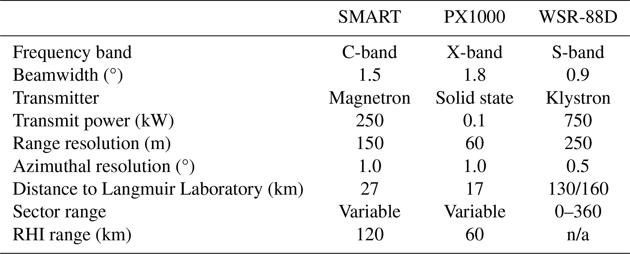
n/a: not applicable.

The SMART radar collected volumes of 20 sector sweeps across a 130° azimuth range at elevation angles between 1.6–22.7°, followed by five range height indicator (RHI) scans (vertical cross-section) spaced 1.5° apart in azimuth and centred over Langmuir Laboratory. The whole volume of sector sweeps and RHI scans was repeated every 5 min. The radar generally came online only after deep convection had initiated.

The PX1000 radar generally came online near the beginning of the flight. Initially, the radar collected volumes consisting of 20 full 360° plan position indicator (PPI) sweeps from 1.6–22.7° in elevation every 5 min. When an echo of interest formed, the PX1000's operating mode was switched to 130° sectors nominally centred over Langmuir Laboratory but rotated in azimuth as needed to adequately follow the storm cell being sampled by the aircraft. The sector scans contained the same elevation tilts as the full 360° volumes, but these were followed by RHI scans up to 35 or 45°, depending on the depth of the echo. If the storm approached the radar, a modified set of elevation tilts of 4.8–28.7° were used to better sample the mid-to-upper portions of the cloud. Each set of tasks was repeated approximately every 5 min to maintain coordination with SR1.

Since the PX1000 uses a low-power solid-state transmitter, pulse compression (Salazar Aquino et al., 2021) is employed when the echoes are more than 11 km from the radar. The pulse compression led to radially oriented artefacts that extended before and after the main precipitation feature and had to be edited manually. If the target storm came closer than 10 km to the radar, a non-compressed waveform was often used. This limited the sensitivity to about 15 dBZ but removed the range artefacts.

Manual editing of the data from both radars is performed to remove ground clutter, noise, and pulse-compression artefacts (PX1000 only) around the features that were sampled by the aircraft.

3.4 Automated cameras

Two automated cameras were developed for the campaign. Each camera instrument comprised a Canon EOS 6D Mark II camera, a UV lens filter, a Raspberry Pi, a Mikrotik wi-fi transmitter and receiver, an 8 Gb secure digital card, and a 2 Tb external hard disk. The camera had an f/1.8 50 mm prime lens giving angles of view of 40, 27, and 46° in the horizontal, vertical, and diagonal respectively, captured within 6240×4160 pixels (Canon, 2023).

The Raspberry Pi computers were running a software stack based on the camera-control software GPhoto2, with a web-based front-end written using the Python Twistd framework for control in the field. Connectivity between the two Raspberry Pis was achieved via Secure Shell over a pair of Mikrotik wi-fi routers (the code repository is available at https://bitbucket.org/ncas_it/camera/src/DCMEX-Deployment/, last access: 2 May 2024).

Time-lapse photographs were stored at intervals of 20 s. Shutter speed, aperture, and ISO were automatically adjusted after every 12 photographs. On all days of camera operation, there was at least one camera located at Socorro Airport. The second camera was sometimes placed at Socorro Airport but was also tested at another location in Socorro and was also placed at Magdalena Airport on a number of days. The location coordinates were automatically logged in the camera's metadata. Instrument scientists additionally recorded the yaw, pitch, and roll of the camera set up on each day.

The time-lapse images provide a useful perspective on the development of the clouds during the aircraft observations and, in addition, can be used to estimate properties such as the heights of the cloud base and cloud top.

4 Complementary data

A number of campaign instruments collected data that require specialised processing before publication. These datasets will be described in future project publications. However, in the meantime, the project team welcomes collaboration with anyone wishing to use the data from the following instruments:

• Laser Ablation Aerosol Particle Time-of-Flight (LAAP-TOF) mass spectrometer. The LAAP-TOF (AeroMegt GmbH) was onboard the aircraft. It identifies the chemical compositions of individual aerosol particles. The system of the LAAP-TOF has been described in detail by Marsden et al. (2016, 2018).

• GRIMM sky Optical Particle Counter (skyOPC) (Grimm and Eatough, 2009). The skyOPC was onboard the aircraft. The instrument measures the size of aerosol particles. Here, the skyOPC was operated in the fast mode for smaller sizes, covering a nominal diameter range of 0.25–3 µm.

• Holographic Cloud Probe (HALOHolo). This instrument was onboard the aircraft. It is an upgraded version of the instrument described by Fugal and Shaw (2009). The instrument can provide a 3D volume image of cloud particles. HALOHolo was the only instrument that was not time synchronised during flight. Instead, it was time synchronised in post processing by correlating its in-canister ambient pressure data with core FAAM pressure data.

• Three-View Cloud Particle Imager (3V-CPI). The 3V-CPI, manufactured by SPEC Inc., is an inlet-based combination cloud particle probe onboard the aircraft. The probe integrates the optics and electronics of a 2D-S probe with the same CPI version described in Sect. 3.1.2. Both the 2D-S and CPI observe particles in the cloudy air that pass down a common sample tube. On occasions, these measurements can be affected by artefacts from the fragmentation of particles on the inlet, so care must be taken to identify and remove these effects by various techniques (Connolly et al., 2007). This is particularly true when the inlet knife edge becomes rimed in highly supercooled liquid water content conditions.

• Backscatter Cloud Probe with Depolarisation (BCP-D). The BCP-D, manufactured by DMT, was onboard the aircraft. It is a miniature backscatter cloud spectrometer based on the original Backscatter Cloud Probe (BCP) described by Beswick et al. (2014). The BCP-D measured cloud droplet size distributions over the size range of approximately 2–50 µm.

• PLAIR Rapid-E+. This instrument was based at Langmuir Kiva-2. It characterises airborne particles between 0.3–100 µm, including bacteria, fungal spores, viruses, pollen, and other aerosols. It used a combination of time-dependent scattered light pattern analysis and fluorescence spectroscopy to provide aerosol shape and surface-morphology signatures (e.g. Lieberherr et al., 2021). Aerosols were sampled via a PLAIR Sigma-2 inlet connected to the sample inlet installed at Kiva-2. The instrument provided basic bio-fluorescent and non-biogenic aerosol concentration size distribution measurements.

• Digitel DPA-14. The Digitel is a programmable filter carousel sampling system to measure INPs. It was based at Langmuir Laboratory.

• Electric field mills. Langmuir Laboratory maintains three E100 electric field mills. There was also a slow antenna of the Langmuir Electric Field Array (LEFA) design located on West Knoll, roughly 1.5 km southwest of Kiva2 (Hager et al., 2012).

5 Dataset archive details

The following subsections provide guidance to those accessing the dataset. Details on the directory structure and the contents of key files are provided based on the different collections of archived data.

5.1 Aircraft data

Individual-flight data collected aboard the FAAM BAe-146 aircraft are archived with the Centre for Environmental Data Analysis (CEDA) (Facility for Airborne Atmospheric Measurements et al., 2024). For a given flight, the top-level files and directories of importance to the vast majority of users are as follows:

• 00README – flight information and active instruments listing

• 00README_catalogue_and_licence.txt – a description of the licence under which the data can be used

• asmm_faam_<flight date>_c<flight number>_fm1.xml – the Airborne Science Mission Metadata file (European Facility for Airborne Research, 2017) that is created for each flight

• flight-report_faam_<flight date>_r<revision number>_c<flight number>.pdf – automatically generated reference document containing the sortie brief, the crew details and flight timings, the flight summary, ground-to-aircraft chat, preliminary quality assurance data plots, pilot weather, in-flight screenshots, and any other ancillary information recorded during the flight

• instrument-report_faam_YYYYmmdd_rN_cNNN.* – automatically generated log of instrument connections to the aircraft network; different file formats are provided

• core_processed – the directory containing FAAM core instrument data

• mo-non-core – the directory containing data post-processed by UK Met Office collaborators

• non-core – the directory containing instrument data from other collaborators.

In the core_processed directory, the files provided are:

• core_faam_<flight date>_v<version number>_r<revision number>_c<flight number>.nc – along with GPS-based position data, aircraft speed, and pressure, this file contains data from the following instruments: CPC-a, the Nevzorov probe, the SEA WCM-2000 probe, and the temperature and humidity probes. Processing for this version number is described by Sproson (2022). We recommend using the processed Nevzorov data in the mo-non-core directory.

• core_faam_<flight date>_v<version number>_r<revision number>_c<flight number>_1hz.nc – this file contains the same instruments as core_faam_<flight date>_v<version number>_r<revision number>_c<flight number>.nc but with data coarsened to 1 Hz frequency.

• core-cloud-phys_faam_<flight date>_v<version number>_r<revision number>_c<flight number>.nc – this file contains data from the following instruments: CIP-15, CIP-100, AIMMS-20, PCASP, and CDP.

• core-cloud-phys_faam_<flight date>_v<version number>_r<revision number>_c<flight number>_<cdp-1 / pcasp-2>_cal.nc – these files contain calibration information for CDP/PCASP particle size bins.

• core-cloud-phys_faam_<flight date>_v<version number>_r<revision number>_c<flight number>_cip<15 / 100>_images.nc – these files contain images from the CIP15/CIP100 instruments.

• faam-dropsonde_faam_<flight date><UTC time of dropsonde>_r<revision number>_c<flight number>_proc.nc – this file contains data from the dropsonde.

• faam-video – this directory contains mp4 files from the on-aircraft cameras. The first part of the filename includes one of “ffc”, “rfc”, “ufc”, or “dfc”, which represent forward-, rearward-, upward-, and downward-facing camera, respectively. The six-digit number in the filename provides the UTC start time of the video.

In the mo-non-core directory, the files provided are:

• metoffice-<twc/nevzorov>_faam_<flight date>_r<revision number>_c<flight number>_<data frequency>.nc – UK Met Office processed data of the total-water probe and Nevzorov. Total-water probe data are available at their measurement frequency and averaged to 1 Hz. We recommend using the processed Nevzorov data in this directory, as it has undergone additional processing compared to that in the core_processed directory.

In the non-core directory, the files provided are:

• man-<2ds / hvps / cpi>_faam_<flight date>_v<version number>_r<revision number>_c<flight number>.nc – these files contain 2D-S, HVPS-3, and CPI particle count data processed by the University of Manchester.

• man-<ams / SP2 / smps>_faam_<flight date>_r<revision number>_c<flight number>.na – these files contain AMS chemical composition concentration, SP2 black-carbon, and SMPS aerosol number size distribution data processed by the University of Manchester. The files use the NASA-Ames (.na) format.

Data from the aircraft INP aerosol filter laboratory analysis, including INP concentrations and the size-resolved particle composition, are available in Daily et al. (2024). This includes csv files containing filter metadata (sampling time, altitude, air volume, flow rate), INP concentrations (both concentrations and freezing temperatures obtained in the droplet freezing experiments), and SEM-EDS data (particle size distribution and EDS data tables in the form of fractional compositions calculated using our classification algorithm).

5.2 Langmuir Laboratory, camera, and radar data

Langmuir Laboratory aerosol data from the GRIMM OPC instrument are archived with CEDA (Williams et al., 2024). There is a netcdf file for each day, which is denoted in the filename with the format YYYYMMDD.

Langmuir Laboratory meteorological data from the two stations described in Sect. 3.2 are archived with CEDA (Flynn and Wu, 2024). There are four csv files in this dataset, two for each station (“gmx600” and “wtx536” in the filenames). The filenames of the two files for a given station indicate the calendar month that the data were collected, using the format YYYYMM.

Ground camera images are archived with CEDA (Finney et al., 2023a, b). The directory structure is of the form 20220621_dcmex/v<version number>/<year>/<month>/<day>/. The filenames contain the date and time (in the format YYYYMMDD-HHmmss) when the image was taken and a location name. The jpg files contain metadata describing the camera location and positioning. A sample of time-lapse videos is archived at Finney et al. (2023c).

Radar data are archived in Carrie et al. (2024). The files from each day of operation are zipped in an archive file. Within those files, each individual radar sweep (sector or range–height indicator (RHI)) is stored with the following naming convention: cfrad.<start day>_<start time>_to_<end day>_<end time>_<radar name>_v<N>_s<n>_<el / az>_<PPI or RHI>.nc. The start day and end day are given in the format YYYYMMDD, and the start time and end time are shown in the format HHmmss.fractionalsecond. “N” is the volume number through the day (consecutive sweeps or RHIs are grouped into a contiguous volume), “n” is the number of the sweep within the volume, “el / az” is the fixed elevation angle of the PPI or the fixed azimuth angle of the RHI respectively, and “PPI or RHI” denotes the orientation of the scan. Each netcdf file contains the radar location along with parameters for that particular scan within the metadata as per the cf-radial file convention (NCAR, 2016).

Figure 5 ERA5 18:00z relative humidity and zonal and meridional winds during the DCMEX campaign. (a) A time–pressure plot created using the mean ERA5 values over 33.5–34.5° N and 106.5–107.5° W (approximately the Magdalena Mountains). Contour lines show 2.5 m s⁻¹ (solid) and −2.5 m s⁻¹ (dashed) winds in the northward (black) and eastward (grey) directions. In the bottom panels, the 700 hPa spatial distributions of relative humidity (filled contours; colour scale is the same as in (a)) and wind (vectors) are shown for two illustrative days, (b) 19 July and (c) 29 July. Grey lines on the map show USA state boundaries and country boundaries. Black lines show coastlines. A purple cross marks the location of the Magdalena Mountains.

6 Case characteristics

The region around the Magdalena Mountains in New Mexico receives the majority of its precipitation in July and August. There is substantial year-to-year variability in the amount and timing of precipitation (Prein et al., 2022). Helpfully, the majority of the days within the campaign were conducive to convective cloud formation over the Magdalenas. In this section, we use the extensive array of operational observation and reanalysis data to explore the general character of the meteorology, aerosol, and clouds across the campaign period.

Using the ECMWF ERA5 reanalysis (Hersbach et al., 2020), Fig. 5 shows that, as the campaign began, there was low-relative-humidity air, with a northerly wind flow moving in on the 19 and 20 July. Between the 19 and 28 July, there was a transition towards a moist southerly flow with a varying easterly component at mid-to-upper levels. From the 28 July to the end of the campaign, mid-levels remained moist. Winds transitioned to a northerly flow around 3 August, with a westerly component at low levels, before returning to the southerly setup again before the end of the campaign.

The 700 hPa maps in Fig. 5 show that the profiles over the Magdalena Mountains were parts of large-scale synoptic systems. The dry northerly winds on the 19 July were associated with anti-cyclonic winds over Arizona to the west of New Mexico. The moist southerly air present through the middle of the campaign was part of a large-scale southeasterly flow across Mexico and Texas. The moist synoptic system described is typical of what is sometimes referred to as the North American Monsoon (Boos and Pascale, 2021).

Table 3 provides a range of statistics for each day of the campaign period. They broadly illustrate the low-level meteorological and aerosol conditions as well as the character of the clouds that formed. The Magdalena Ridge Observatory maintains a weather station near Langmuir Laboratory, and New Mexico Tech have shared the operational data collected during the DCMEX campaign. Table 3 includes the mean temperature and dewpoint temperature between 15:00–16:00z (09:00–10:00 a.m. local time) from that station. This time period was chosen to represent the conditions prior to cloud formation. It is also roughly around the time the aircraft took off. The temperatures were highest when the campaign began; they dropped after the 20 July and then stayed fairly steady until the end of the campaign. Meanwhile, the dewpoint temperature increased after 22 July, consistent with the increased low-level relative humidity seen in Fig. 5 around the same time.

As described in Sect. 3.2, surface aerosol stations were installed for the campaign on top of the mountain (Williams et al., 2024). Table 2 shows the total aerosol concentration and the concentration for particles larger than 2.5 µm, as measured by the ground-based GRIMM OPC. Broadly speaking, the concentration of larger aerosol particles followed the total aerosol concentration and was only a small proportion of the total aerosol (∼0.1 %). Notably high aerosol days include 23 July, which saw the first thunderstorm of the campaign, and 7 August, which saw one of the more intense thunderstorms during the later portion of the campaign. Notably low aerosol days include 31 July, which followed the day with the most intense thunderstorm and saw a later start to lightning flashes than on several of the preceding days.

Table 3 Ground-based aerosol and weather measurements and satellite estimates of cloud top height and lightning. Aerosol was obtained by the GRIMM instrument located at Langmuir Laboratory. Temperature (T) and dewpoint temperature (T_d) were obtained from the operational weather station at the Magdalena Ridge Observatory. Temperature at the lifting condensation level (LCL) was estimated from the temperature and dewpoint. All ground-based measurements and estimates are averaged over the hour 15:00–16:00z to represent the conditions prior to convection. Satellite data are processed for the 15:00–21:00z (6 h) period to roughly represent the flight period. Estimates of cloud top height are taken as the maximum GOES value within a rectangular region with edges passing through the points of the kite in Fig. 1, based on 5 min images when available. Only clouds with an optical depth >23 and cloud-top pressure <440 hPa are considered, consistent with the International Satellite Cloud Climatology Project (ISCCP) definition of deep convective cloud. The GOES cloud fields were corrected for parallax shift as described in Fig. 1. Lightning flashes within a rectangular box whose corners are the mid-points of the kite edges in Fig. 1 were counted by the GOES GLM instrument. The number of flashes within 15:00–21:00z as well as the time of first flash are given.

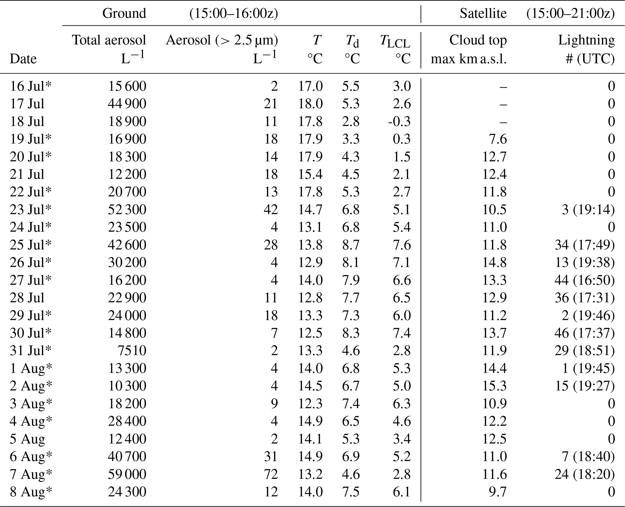
* Flight day.

With a focus on the microphysical behaviour of the clouds, we will explore the role of cloud base temperature in influencing cloud processes. To provide an overview of the cloud base temperature across the campaign, we consider an estimate of the lifting condensation level temperature (T_LCL) relative to the Magdalena Observatory surface observations of temperature, dewpoint temperature, and pressure. T_LCL was calculated using the MetPy Python package (May et al., 2022). For cumulus developing into deep convection, we consider that T_LCL is a reasonable approximation of the cloud base temperature.

LCL temperature remained low, and close to 0 °C, at the beginning of the campaign. It then warmed substantially to around 5–8 °C between 23 July and 3 August, with the exception of a dip to 2.8 °C on 31 July. Between 4 and 8 August, the LCL temperature fluctuated with a range between 2.8 and 6.1 °C.

There is a broad relation between these cloud base temperatures and three measures of the deep convective storm characteristics. Initially, we considered the maximum deep convective cloud top height, the time of first lightning, and number of lightning flashes. We focused on the period 15:00–21:00z, as this was the main period of storm activity on the mountain and when aircraft flights and other observations were carried out.

Maximum cloud top heights of cloud with a high optical depth (i.e. optical depth >23, cloud top pressure <440 hPa) ranged between 7.6 and 15.3 km a.s.l. Based on this definition, the highest clouds occurred on 26 July and on 1 and 2 August. Generally, the middle of the campaign saw higher cloud tops, consistent with these clouds electrifying. The earliest lightning flash measured by the GOES GLM instrument was at 17:31z (11:31 local time) on 28 July. This was a down day for the aircraft. However, early lightning flashes also occurred on 25, 27, and 30 July, and these days also had the highest number of flashes between 15:00–21:00z.

The information in this section demonstrates that in situ observations have been obtained for a wide range of summertime convective conditions. The dataset includes days with relatively dry as well as relatively moist conditions, weakly and strongly electrified clouds, days when convection did not establish, and days when convection was deep. In addition, there are a number of days with high aerosol loading and others with relatively low aerosol. As a result, a variety of case studies can be chosen depending on the scientific question of interest.

7 Data availability

Aircraft data are available for the DCMEX flights c297–c315 at https://doi.org/10.5285/B1211AD185E24B488D41DD98F9 57506C (Facility for Airborne Atmospheric Measurements et al., 2024). The majority of the ground-based instrument data are also included in that collection (Finney et al., 2023a, b; Flynn and Wu, 2024; Williams et al., 2024). Two datasets are not archived with CEDA: radar and aircraft INP filter data. Radar data are available at https://doi.org/10.5281/zenodo.10472266 (Carrie et al., 2024). INP filter data are available at https://doi.org/10.5518/1476 (Daily et al., 2024). ERA5 data were accessed through the CEDA archive (European Centre for Medium-Range Weather Forecasts, 2021).

8 Summary

The DCMEX campaign has collected a wide range of observation data of convective cloud growth in New Mexico over the period July–August 2022. Collected data included measurements of aerosol, cloud physics, radar signals, and thermodynamic and dynamic variables. In addition, a collection of time-lapse imagery of the cloud growth was obtained.

The study was focused over the Magdalena Mountains, where reliable orographic convection occurs during the summer. Convective cloud growth was observed on 17 of the 19 flight days. Day-to-day environmental conditions varied in terms of source air mass, humidity, and wind shear. As a result, the dataset includes convective cloud forming at a range of speeds and intensities. The range of data allows analysis of primary- and secondary-ice formation under different conditions and, when combined with modelling and operational satellite data, the dataset enables analysis of the influence of microphysical processes on the cloud radiative effect.

This paper has introduced the details of the campaign and dataset that will enable researchers external to the project to use the DCMEX observation data. The dataset offers opportunities to understand aerosol–cloud interactions and cloud physics and can be used with modelling and operational data to understand the cloud radiative effect.