Spatial and temporal stable water isotope data from the upper snowpack at the EastGRIP camp site, NE Greenland, sampled in summer 2018

Stable water isotopes stored in snow, firn and ice are used to reconstruct climatic parameters. The imprint of these parameters at the snow surface and their preservation in the upper snowpack are determined by a number of processes influencing the recording of the environmental signal.

Here, we present a dataset of approximately 3800 snow samples analysed for their stable water isotope composition, which were obtained during the summer season next to the deep drilling site of the East Greenland Ice Core Project in northeast Greenland (75.635411° N, 36.000250° W). Sampling was carried out every third day between 14 May and 3 August 2018 along a 39 m long transect. Three depth intervals in the top 10 cm were sampled at 30 positions with a higher resolution closer to the surface (0–1 and 1–4 cm depth vs. 4–10 cm). The sample analysis was carried out at two renowned stable water isotope laboratories that produced isotope data with the overall highest uncertainty of 0.09 ‰ for δ¹⁸O and 0.8 ‰ for δD.

This unique dataset shows the strongest δ¹⁸O variability closest to the surface, damped and delayed variations in the lowest layer, and a trend towards increasing homogeneity towards the end of the season, especially in the deepest layer. Additional information on the snow height and its temporal changes suggests a non-uniform spatial imprint of the seasonal climatic information in this area, potentially following the stratigraphic noise of the surface.

The data can be used to study the relation between snow height (changes) and the imprint and preservation of the isotopic composition at a site with 10–14 cm w.e. yr⁻¹ accumulation. The high-temporal-resolution sampling allows additional analyses on (post-)depositional processes, such as vapour–snow exchange. The data can be accessed at https://doi.org/10.1594/PANGAEA.956626 (Zuhr et al., 2023a).

1 Introduction

Stable water isotopes measured in ice cores are widely used as proxies for past temperatures (e.g. Dansgaard, 1964; Jouzel et al., 2003; Brook and Buizert, 2018). For reliable reconstructions, it is essential to understand the processes occurring during the signal formation and imprint as well as the modifications of the signal during preservation.

Snowfall above ice sheets contains a signature of the atmospheric temperature. Snowfall itself can be intermittent in space and time (e.g. Persson et al., 2011) and might after the initial deposition be affected by wind erosion, leading to mass redistribution to other positions (e.g. Li and Pomeroy, 1997a, b; Filhol and Sturm, 2019). Snow erosion and redeposition are not spatially homogeneous but influenced by surface features, such as dunes and sastrugi (e.g. Fisher et al., 1985; Picard et al., 2019; Zuhr et al., 2021b). Hence, accumulation is characterised by the seasonality of snowfall, the meteorological conditions, e.g. wind speed and direction, and the stratigraphic features at a specific site.

Accumulation intermittency influences the recording of the environmental information and introduces a significant amount of noise to the proxy time series (e.g. Casado et al., 2018, 2020). The isotopic signal is imprinted during the formation of precipitation. After snow is deposited, this signal can be significantly modified by post-depositional processes occurring through exchanges between snow (e.g. Steen-Larsen et al., 2014; Dadic et al., 2015; Ritter et al., 2016; Wahl et al., 2022) and the atmosphere or within the snow column, i.e. isotopic diffusion (Johnsen et al., 2000).

Comparison of isotopic records sampled on snow trenches revealed a large spatial variability of the snowpack and firn column, which causes a low signal-to-noise ratio of the proxy data, i.e. stable water isotopes, and associated stratigraphic noise in regions of low accumulation (e.g. Münch et al., 2016, 2017). Repeatedly sampled snow profiles with additional information on the snow height at each sampling location illustrated the buildup of this stratigraphic noise and the associated noise in the isotope data (Zuhr et al., 2023b). However, questions still exist on the signal contribution from precipitation, vapour–snow exchange and other processes relevant for the isotope ice core signal.

In recent years, (modelling and observational) studies have considered a number of processes, such as precipitation intermittency and diffusion (Casado et al., 2020), vapour–snow exchange (e.g. Touzeau et al., 2018; Hughes et al., 2021; Wahl et al., 2022), and snow redistribution (Libois et al., 2014). These and many other studies have contributed to pinning down the processes which are not fully understood yet and need better quantification. Thus, the motivation for this study is to answer questions regarding (post-)depositional modifications of the isotopic composition in surface snow, the representativeness of individual snow profiles, and ultimately the preserved signal in the upper snowpack, firn and ice in the end. To answer these questions, the following dataset is a case study that provides insights into the spatial and temporal variability of stable water isotopes in the upper snowpack.

2 Description of the dataset

2.1 Study area

Snow sampling was performed in a clean snow area next to the campsite of the East Greenland Ice Core Project (EastGRIP) in the accumulation zone of the Greenland ice sheet (75.635411° N, 36.000250° W; 2708 m a.s.l.; Fig. 1a). An automatic weather station (AWS) was installed in the vicinity of the study site (Fig. 1b) in 2016 by the Programme for Monitoring of the Greenland Ice Sheet (PROMICE) and provides continuous meteorological data (Fausto and van As, 2019). The study area is characterised by an annual temperature of −26.5 °C (daily averages between −61.6 and −1.9 °C) and average wind speed of 5.5 m s⁻¹ (daily averages between 1.6 and 11.2 m s⁻¹) mainly from WSW (240°) for the year 2018 based on data from the PROMICE AWS. The mean accumulation rate ranges around 10–14 cm w.e. yr⁻¹ (Schaller et al., 2016; Karlsson et al., 2020).

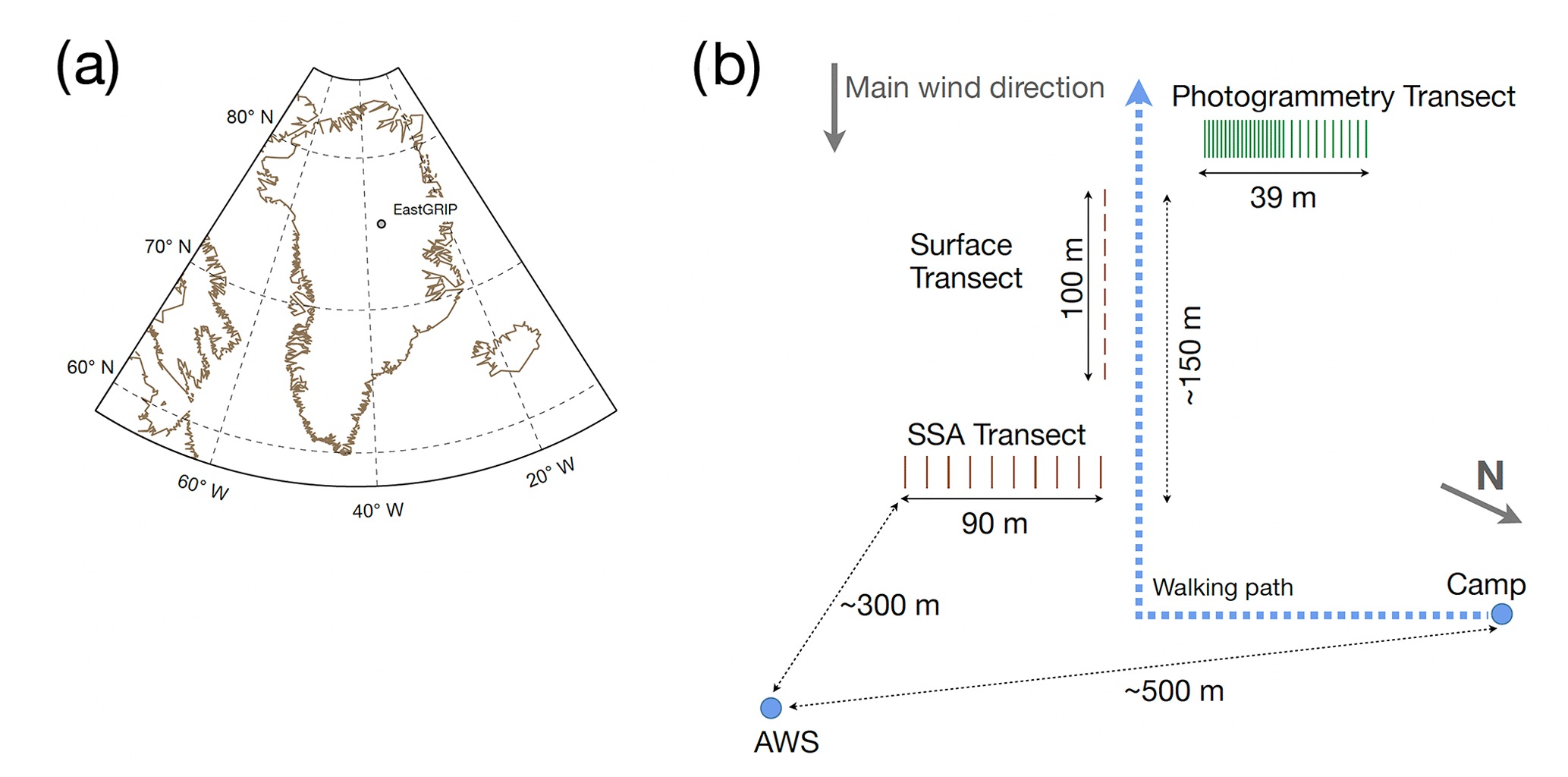
Figure 1 The location of the study site next to the EastGRIP camp site is illustrated in (a). The organisation of the study site in 2018 is shown in (b) including the snow height measurement and the snow sampling. Specific surface area (SSA) and surface transect are used in complementary studies and mentioned in Sect. 4.2.

2.2 Snow sampling

Snow sampling was carried out at 30 positions along a 39 m long transect (Fig. 2) every 3 d between 14 May and 3 August 2018. The sampling positions had a spacing of 1 m for the first 20 positions and 2 m for the remaining 10 positions (Fig. 2a). The individual positions were marked with green glass-fibre sticks which were also used for the additional photogrammetry study performed at the same site during the same observation period (Fig. 2c). Each sampling position was additionally marked with a tiny wooden stick. To avoid resampling of the exact same snow and redistribution caused by the sampling itself, the sampling position moved each time some centimetres towards the wind direction.

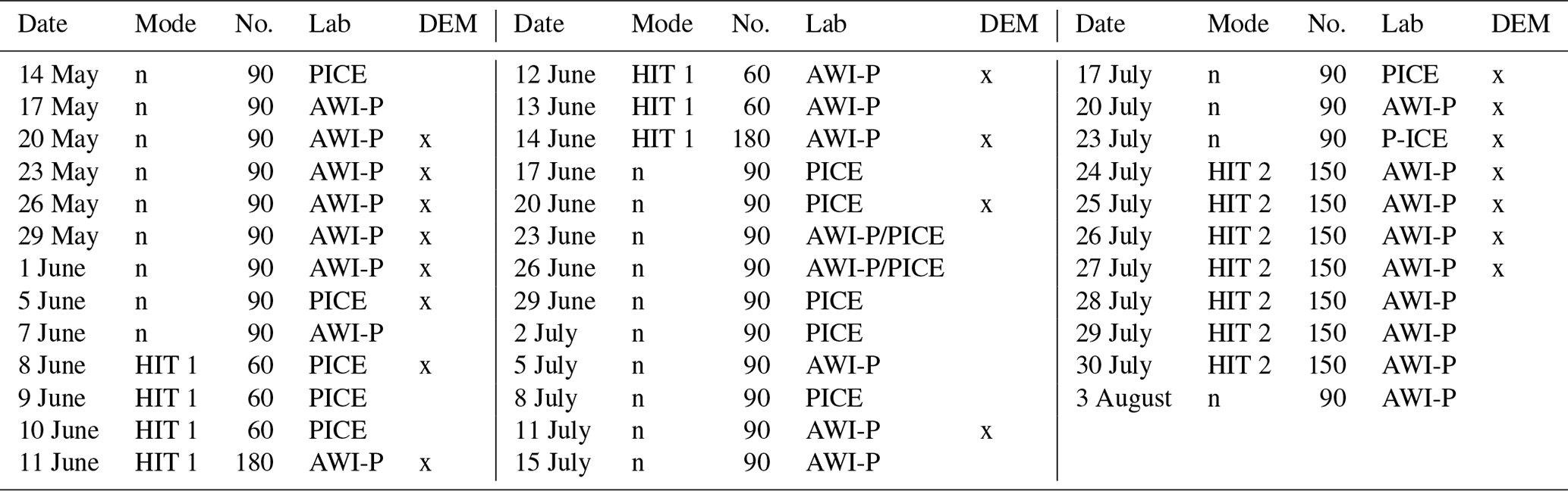
Three samples were taken at each position (0–1, 1–4 and 4–10 cm in the normal mode n, Fig. 2b), stored airtight in high-purity sampling bags (^®Whirl-Paks) and transported to Germany in a frozen state. During two periods, sampling was performed every day for 7 consecutive days with six sampled depth layers and is referred to as high-intensity sampling (HIT). These periods were chosen based on the meteorological conditions during the acquisitions. The HIT 1 period, from 8 to 14 June 2018, followed a major snowfall event to study the signal imprint from the surface penetrating into the upper snowpack. During that period, samples were collected only at 10 sampling positions due to time constraints. The sampled depth intervals were 0–1, 1–2, 2–4, 4–6, 6–8 and 8–10 cm (Fig. 2b) at the positions 1, 6, 11, 16, 20, 22, 24, 26, 28 and 30. The second high-resolution sampling period (HIT 2) was from 24 to 30 July 2018, covering a snowfall-free period to focus on vapour–snow exchange processes. A total of 25 positions were sampled (positions 1–10, 12, 14, 16, 18, 20–30) with the following depth intervals: 0–0.5, 0.5–1, 1–2, 2–4, 4–6 and 6–10 cm. The vertical resolution was changed in order to obtain a higher sampling resolution closer to the surface where most changes are expected due to (post-)depositional processes (Hughes et al., 2021; Wahl et al., 2022). Respective days with the different snow sampling schemes are also listed in Table 1.

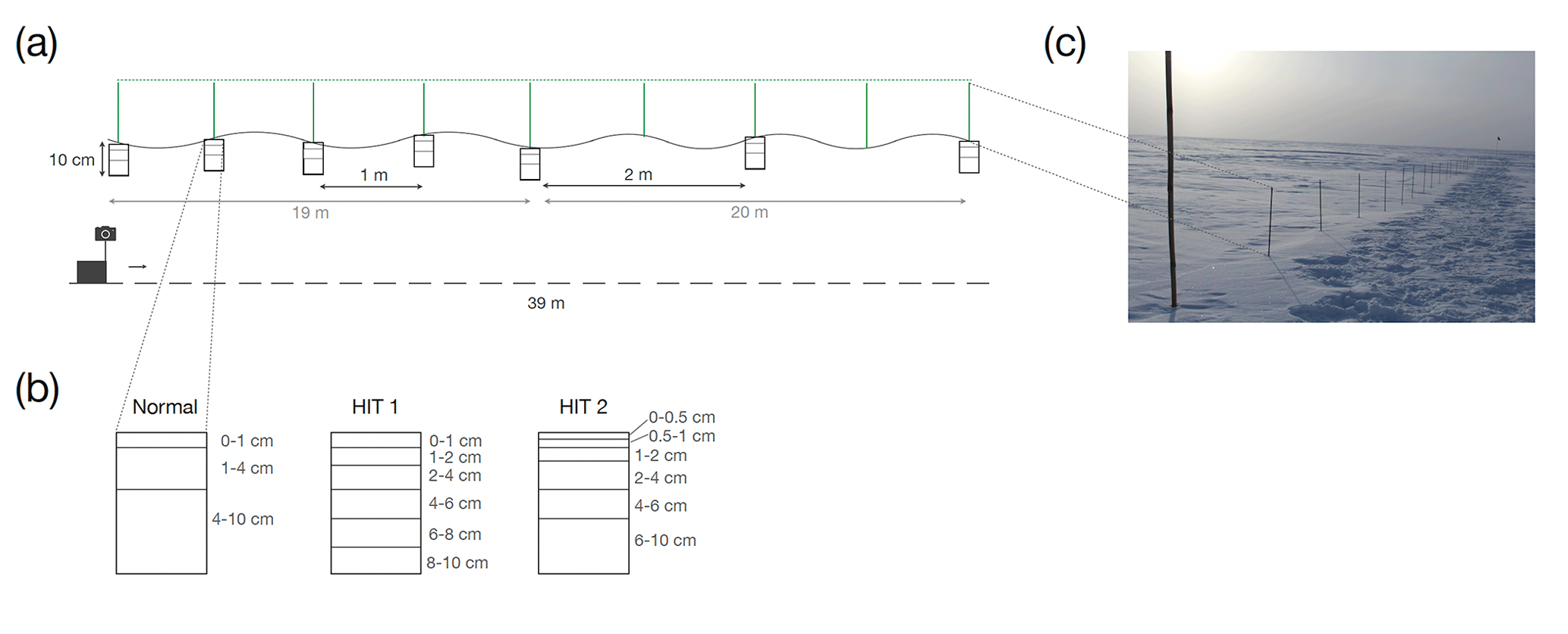
Figure 2 The sampling setup showing the snow sampling and the snow height measurement is illustrated in (a). Snow was sampled for three depth layers (0–1, 1–4 and 4–10 cm) during the normal mode (n) as shown in (b). During the high-intensity sampling modes (HIT 1 and HIT 2) six depth layers were sampled as indicated and detailed in Table 1. Glass-fibre sticks as shown in (a) and (c) were used for indications of the sampling positions as well as for georeferencing of the photogrammetry. The dashed horizontal line indicates that all glass-fibre sticks were levelled to the same height.

Table 1 Detailed information on the sampling days (date in 2018), the respective mode (Mode; n: normal, HIT 1: high-intensity sampling scheme 1, HIT 2: high-intensity sampling scheme 2; explained in the text and Fig. 2b) for each sampling, the number of samples (No.), the laboratory that performed the measurements (Lab; AWI-P: AWI Potsdam, PICE: Physics of Ice, Climate and Earth, University of Copenhagen, Denmark) and the availability of a digital elevation model (DEM) from Zuhr et al. (2021b).

2.3 Stable water isotope measurements

Stable water isotope measurements were performed in two laboratories. For most sampling days, all samples were measured in one laboratory. Only 2 sampling days were split and measured in both laboratories (i.e. 23 and 26 June 2018). Table 1 indicates for each sampling day in which laboratory the measurement was performed.

About 70 % of the stable water isotope measurements were performed in the ISOLAB Stable Isotope Facility at the Alfred Wegener Institute (AWI) in Potsdam, Germany, using a Picarro Inc. cavity ring-down spectrometer (model L2140-i) with a high-precision vaporiser (A0211) and autosampler (A0325). The measurement protocol was adjusted to the expected range of isotope values. Hence, the number of injections for samples and reference waters was three, except for the initialisation block at the beginning of the measurement sequence with standards which were injected six times. All data were calibrated to the VSMOW-SLAP scale. A post-run correction, including memory and drift correction as well as normalisation and calibration, was performed following van Geldern and Barth (2012) using the calibration algorithm described in Münch et al. (2016). The measurement uncertainty of this specific analysis is derived from an independent control reference water which was measured during each run but not used for the calibration. The root mean square deviation of the difference between the expected and the measured values is used as a measure of uncertainty and is 0.09 ‰ for δ¹⁸O and 0.8 ‰ for δD.

The remaining ∼ 30 % of the samples were measured in the Stable Isotope Laboratory of the Institute for Physics of Ice, Climate and Earth (PICE), Niels Bohr Institute, at the University of Copenhagen in Copenhagen, Denmark. A cavity ring-down spectrometer from Picarro Inc. (model L2140-i) was used as well but using a high-throughput low-volume vaporiser (Picarro-A0212 – discontinued model as of 2016). The initialisation block at the beginning of the sequences was injected 20 times per reference water. The number of injections for all successive samples was four. A detailed list of the injection protocol is provided in Table 3 in Gkinis et al. (2021). No memory correction was applied since the high-throughput vaporiser reduced the amount of memory in the cavity to a level that no correction is necessary for a 12 h measurement run (Gkinis et al., 2021). The data were calibrated on the VSMOW-SLAP scale. These measurement runs also contained an independent reference water used to estimate the uncertainty, which is 0.04 ‰ for δ¹⁸O and 0.33 ‰ for δD.

All isotopic ratios are reported in per mill (‰) following the delta notation:

$$\begin{array}{}\text{(1)}& \mathit{\delta }=\left({\displaystyle \frac{R_{\mathrm{sample}}}{R_{\mathrm{reference}}}}\right)-\mathrm{1}\end{array}$$

(Craig, 1961), with R_sample as the isotopic ratio of the sample and R_reference the ratio of an in-house reference water which is calibrated against the international VSMOW-SLAP scale. The second-order parameter deuterium excess was calculated from the data following

$$\begin{array}{}\text{(2)}& \text{d-excess}=\mathit{\delta }D-\mathrm{8}\cdot {\mathit{\delta }}^{\mathrm{18}}O.\end{array}$$

Cross-measurements between the two laboratories were performed by measuring the same samples and reference waters in both laboratories using their respective methods. The samples were kept frozen until the distribution into glass vials at the laboratory at AWI in Potsdam, Germany. The vials were not filled completely but had a small headspace, as is the usual practice in this laboratory. The vials were kept cold during the transport to PICE in Copenhagen, Denmark, to avoid any exchange between the headspace and the water. The raw data were calibrated in each laboratory following their usual procedure as described above. The comparison resulted in a root mean square deviation of 1.45 ‰ for δ¹⁸O and 1 ‰ for δD.

2.4 Meteorological conditions during the 2018 summer season

The observation period between 14 May and 3 August 2018 was characterised by a mean temperature of −14.3 °C (hourly averages between −30.6 and +0.3 °C; Fig. 3). The average wind speed was 4.1 m s⁻¹ (hourly maximum values up to 11.7 m s⁻¹) from a west-southwest direction (236°±42°). The latent heat flux shows a diurnal cycle with a maximum during the day and a minimum during night. Strong fluxes are observed, for instance, between 4 and 9 June and are accompanied by an increase in temperature and specific humidity.

Conditions favourable for snowdrift events, i.e. 100 h average wind speed above 4 m s⁻¹ (Groot Zwaaftink et al., 2013), were present for 49 % of the time. Snowfall was manually documented on 29 d during the 80 d long observation period (Fig. 3). No manual documentation of snowdrift events was performed.

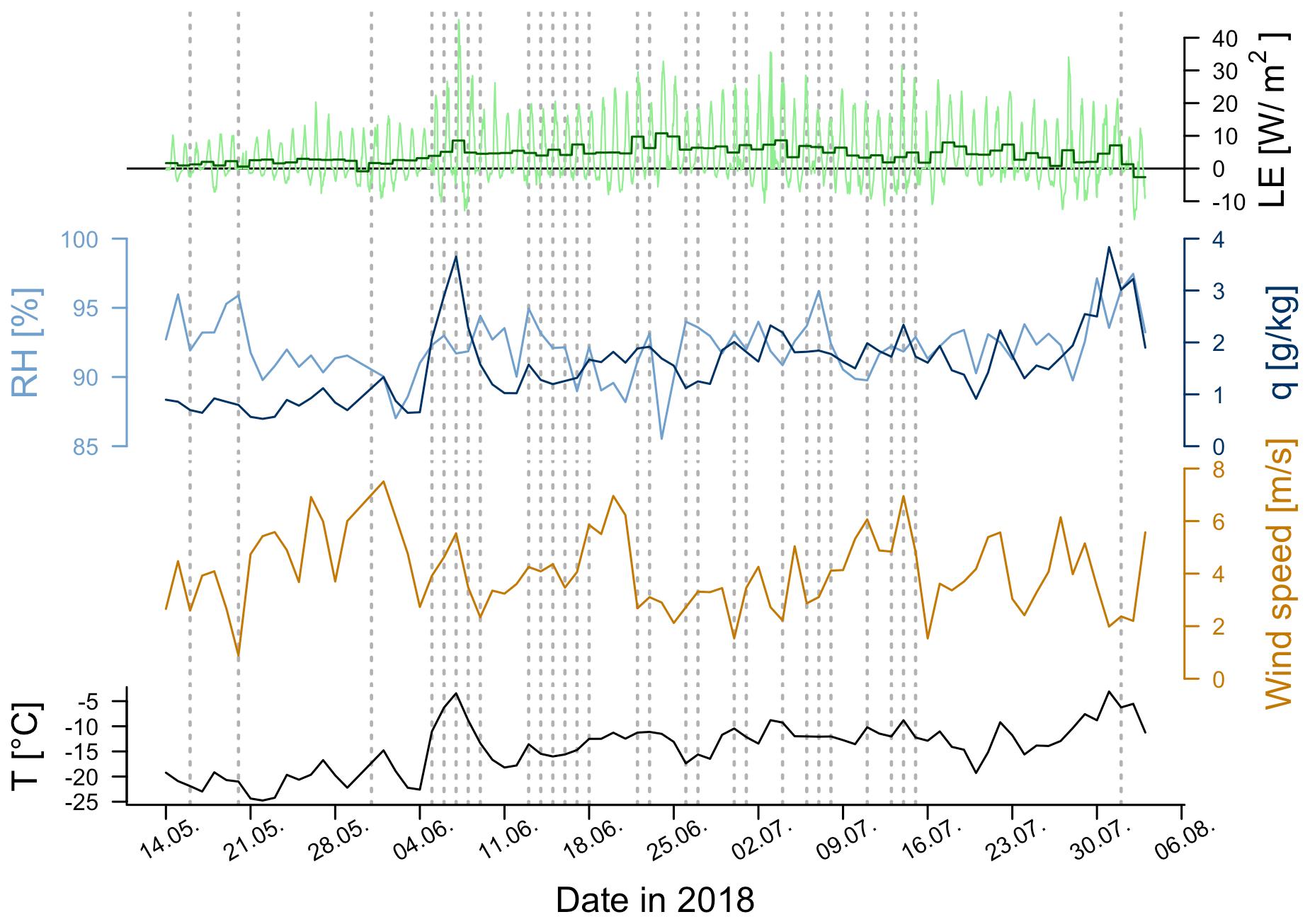
Figure 3 Meteorological conditions during the observation period from 14 May to 3 August 2018 from the PROMICE weather station (Fausto and van As, 2019). The 10 min high-resolution data are averaged to daily values for relative humidity with respect to ice (RH), specific humidity (q), wind speed and temperature (T). The data showing latent heat flux (LE) are averaged to hourly (light green) and daily values (i.e. net LE, dark green). Vertical grey lines show manually documented snowfall events (n=29) throughout the observation period.

3 Results

3.1 Description of the data

The dataset consists of 3777 individual snow samples and hence isotope data points which were sampled on 37 d between 14 May and 3 August 2018 (Table 1). The δ¹⁸O data have a right-skewed distribution and span a range from −44.6 ‰ to −22.7 ‰ with a mean of −32.6 ‰ and a standard deviation of 3.4 ‰ (Fig. 4a). The uppermost sampled layer (0–1 cm) has the highest δ¹⁸O values, while the deepest sampled layer (4–10 cm) contains the lowest values on average with an absolute minimum value of −44.6 ‰ (Fig. 4a). The standard deviation across all samples for one depth layer increases from 2.3 ‰ for the uppermost layer to 3.4 ‰ for the layer from 1–4 cm and to 4.2 ‰ for the lowest layer. The range of individual δ¹⁸O values is largest for the interval 1–4 cm at 21 ‰ compared to 16.8 ‰ for 0–1 cm and 17.3 ‰ for 4–10 cm.

Individual values for the second-order parameter d-excess range from −9 ‰ to 24.6 ‰ (Fig. 4b). Values for the sampled depth layer are highest for the surface layer with an overall mean of 11.4 ‰ (ranges between −2.3 ‰ and 24.6 ‰). The following layers have mean values of 6 ‰ (ranges between −9 ‰ and 18.8 ‰) and 4.6 ‰ (ranges between −5 ‰ and 14.5 ‰) for the lowest layer.

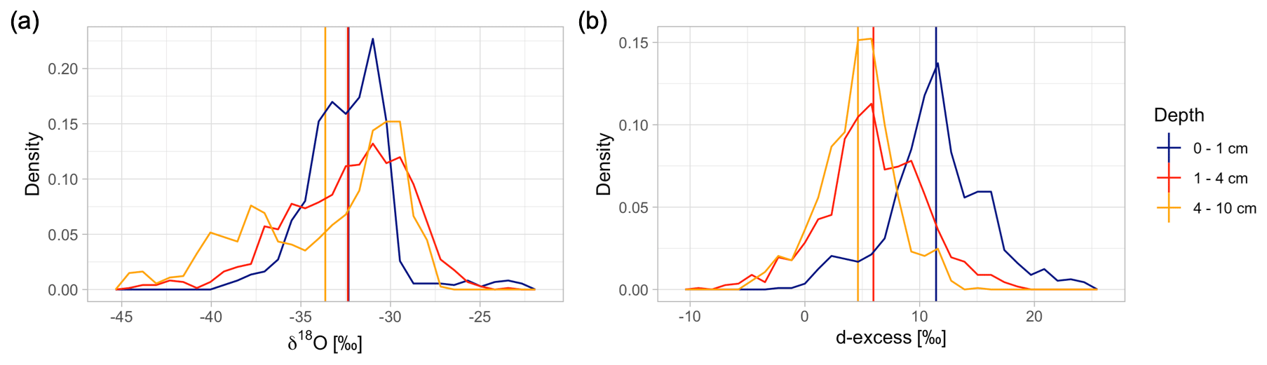
Figure 4 Distribution of individual samples δ¹⁸O and d-excess values from the normal sampling mode as well as averages from the high-resolution samplings per depth layer over the whole season. The vertical lines indicate the respective mean for each sampled depth layer.

The dataset is archived on PANGAEA (Zuhr et al., 2023a) and contains columns indicating the sampled depth interval (“Depth layer ice/snow” with the values 1, 2 and 3 indicating the layers 0–1, 1–4 and 4–10 cm), the average sample depth (“Depth ice/snow [m]” with the values 0.005, 0.025 and 0.07 m for the three respective layers) and the relative depth derived from additional information on the surface height (“Depth rel.” in metres with data from Zuhr et al., 2021a). The sampling position along the transect is indicated (“Position” with numbers from 1 to 30) as is the absolute distance along the transect (“Dist [m]”).

3.2 Spatial and temporal variability of δ¹⁸O

The overall standard deviation for the δ¹⁸O values increases from 2.2 ‰ to 2.7 ‰ to 3.2 ‰ with depth from the surface to the deepest layer (variances of 4.8 ‰², 7.0 ‰² and 10.2 ‰², respectively). The evolution of the isotopic composition (Figs. 5 and 6) is characterised by a large increase in δ¹⁸O in the surface and subsurface layers around 5 June after a snowfall event (Fig. 3), which also affected the lowest sampled layer. The strong increase in δ¹⁸O values for the surface layer between 1 and 7 June is recorded in the deeper layers with a damped magnitude, while the following drop is not represented in the deepest layer at all. This period was also characterised by snowfall and warm temperatures (Fig. 3). The middle layer (1–4 cm) shows the highest δ¹⁸O composition in the period between 10 June and 11 July, while the surface layer (0–1 cm) has on average lower values. The second and the third depth layers, i.e. 1–4 and 4–10 cm, show large spatial variability in May with a decreasing trend towards the end of the observation period (Fig. 5). These low values persist until mid-July at the positions between 10 and 14 m, possibly due to the underlying topography.

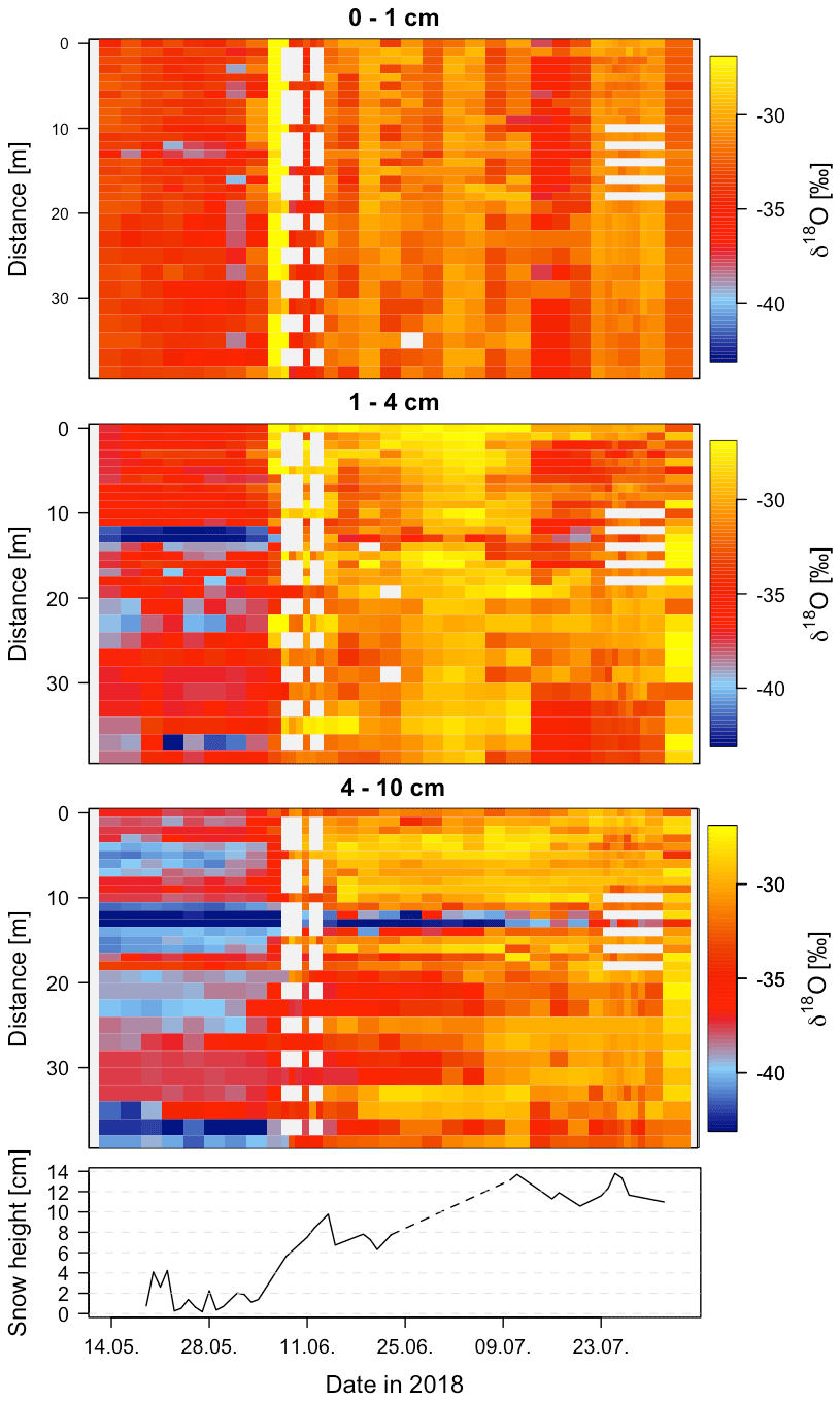
Figure 5 Spatial and temporal representation of the δ¹⁸O data for the three sampled depth layers and all sampling days. The date is given in DD.MM. of the year 2018. The high-resolution sampling periods from 8 to 14 June and 24 to 29 July (Table 1) are visible by variations in the spatial sample coverage (white areas) and are averaged to the depth layers of the normal sampling scheme. The bottom panel shows the evolution of the snow height in the same area during the same time period based on digital elevation models from Zuhr et al. (2021a).

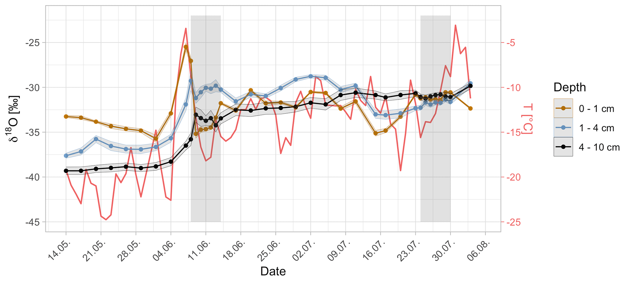
Figure 6 Temporal evolution (date in 2018) of the spatially averaged δ¹⁸O information and the daily temperature (red line, from the nearby AWS). Each data point is an average across 30 samples along the 39 m long transect. The shading shows the standard error. High-resolution sampling periods are averaged to the overall sampling resolution and are indicated with grey bars.

3.3 Spatial and temporal variability of d-excess

The individual depth layers have similar variability in d-excess with standard deviations of 4.4 ‰, 4.3 ‰ and 3.2 ‰ from the top to the bottom layer (Fig. 7, variances of 14.9 ‰², 6.2 ‰² and 1.8 ‰², respectively). The highest d-excess values are observed in the top layer on 26 June 2018, coinciding with snowfall events (Fig. 3), while the layer from 1–4 cm is characterised by lower and partly negative values at the same time. After the snowfall, d-excess in the top layer decreases with time but remains higher than in the layers beneath.

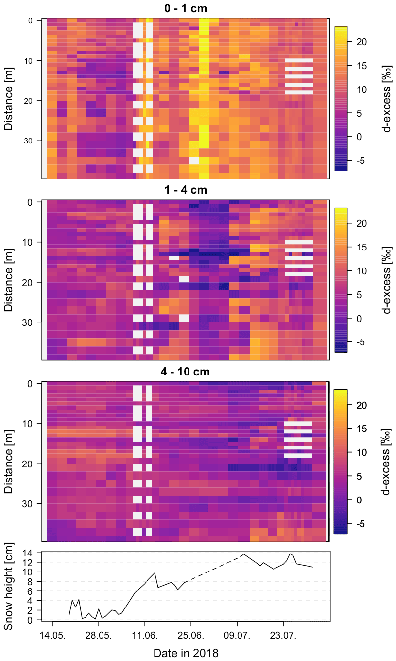
Figure 7 Spatial and temporal representation of the d-excess data for the three sampled depth layers and all sampling days. The date is given in DD.MM. of year 2018. The high-resolution sampling periods from 8 to 14 June and 24 to 29 July (Table 1) are visible by white spots due to a reduced spatial sampling coverage. The bottom panel shows the evolution of the snow height in the same area during the same time period based on digital elevation models from Zuhr et al. (2021a).

The layer from 4–10 cm depth has the lowest variability spatially and also temporally (Fig. 8) with only slight changes between 1.9 ‰ and 7.2 ‰ throughout the observation period. The top layer from 0–1 cm shows the strongest variability with averaged values above 20 ‰. The lowest d-excess values around 0 ‰ are observed in the layer from 1–4 cm during the end of June and beginning of July, which seem to coincide with a large spike in the surface layer d-excess.

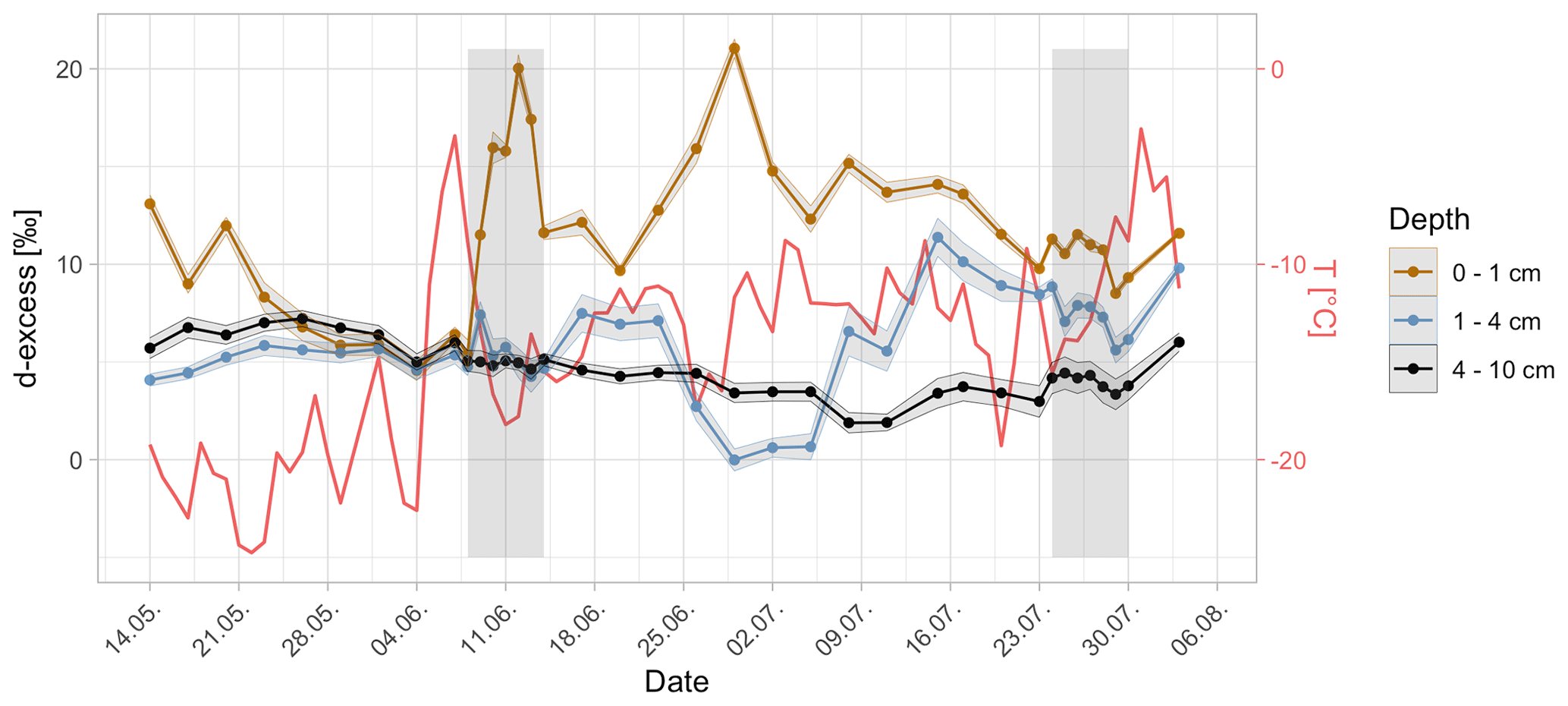
Figure 8 Temporal evolution (date in 2018) of the spatially averaged d-excess and the daily temperature (red line, from the nearby AWS). Each data point is an average across 30 samples along the 39 m long transect. The shading shows the standard error. HIT periods are averaged to the overall sampling resolution of three depth layers and indicated with grey bars.

3.4 High-resolution sampling periods

The first high-resolution sampling period (HIT) started on 8 June after snowfall events during the previous days (Fig. 3) with comparably warm temperatures. Snowfall-free days with low wind speeds (Fig. 3) followed afterwards. δ¹⁸O shows a drop in the surface layer (0–1 cm) and a smaller drop in the layer from 1–2 cm, while the layers beneath show less temporal variability (Fig. 9). Similarly, the surface layer shows the largest changes in d-excess (5.4 ‰ to 20 ‰), while the values in the layers from 1–10 cm remain almost constant (ranging between 2.9 ‰ and 9.2 ‰).

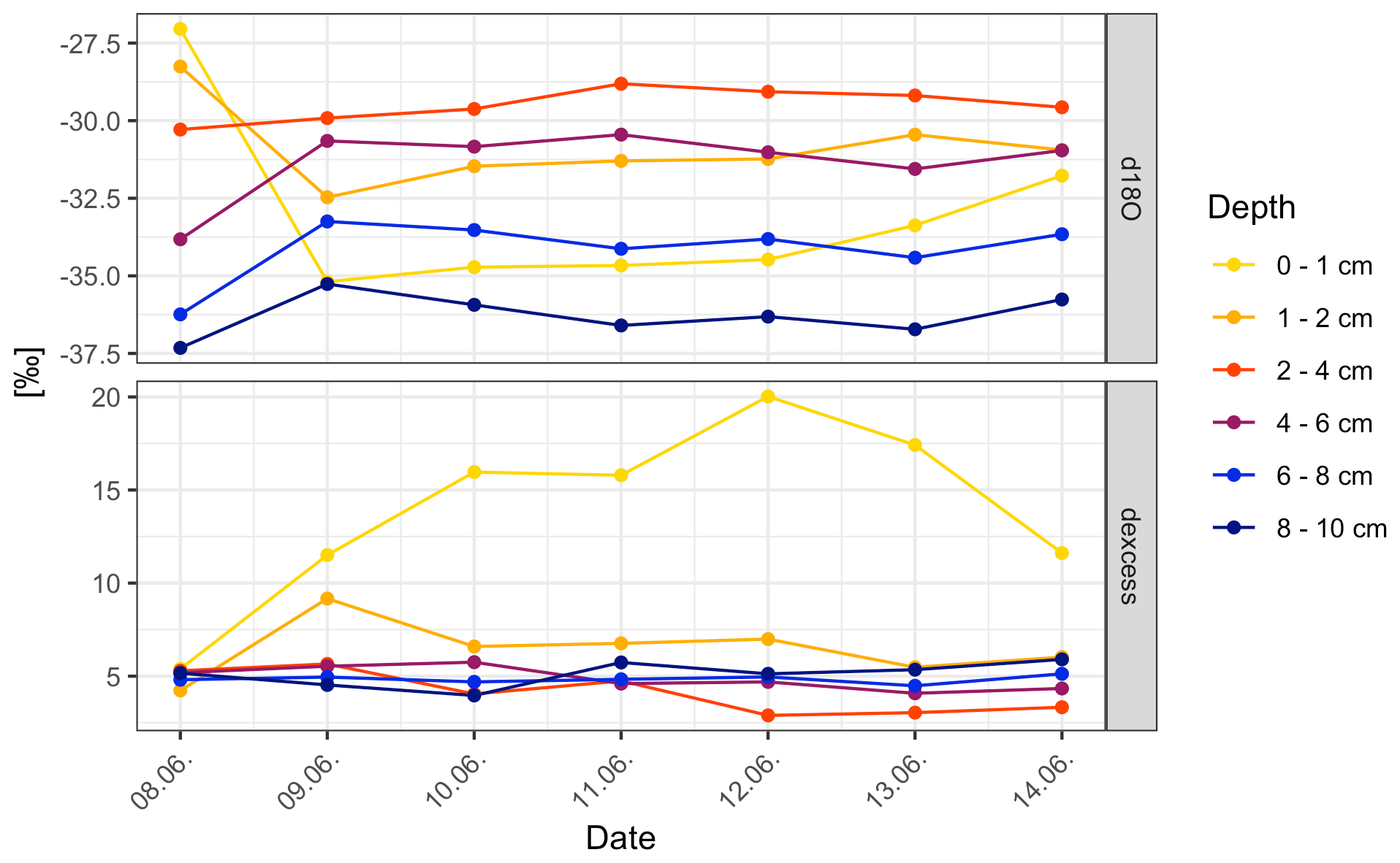
Figure 9 Spatial average δ¹⁸O and d-excess values during the first HIT period from 8 to 14 June 2018. The colour code indicates the sampled depth layer. On 11 and 14 June, samples were taken at all 30 positions, while on the other days they were taken at only 10 positions.

The isotope composition during the second HIT period (Fig. 10) is characterised by small variations in δ¹⁸O with time and slight differences between the individual layers. The overall range of averaged δ¹⁸O per depth layer is small with values between −32.6 ‰ and −30.3 ‰. The d-excess values, however, show a larger spread across the sampled layers (between 2.1 ‰ and 14.2 ‰).

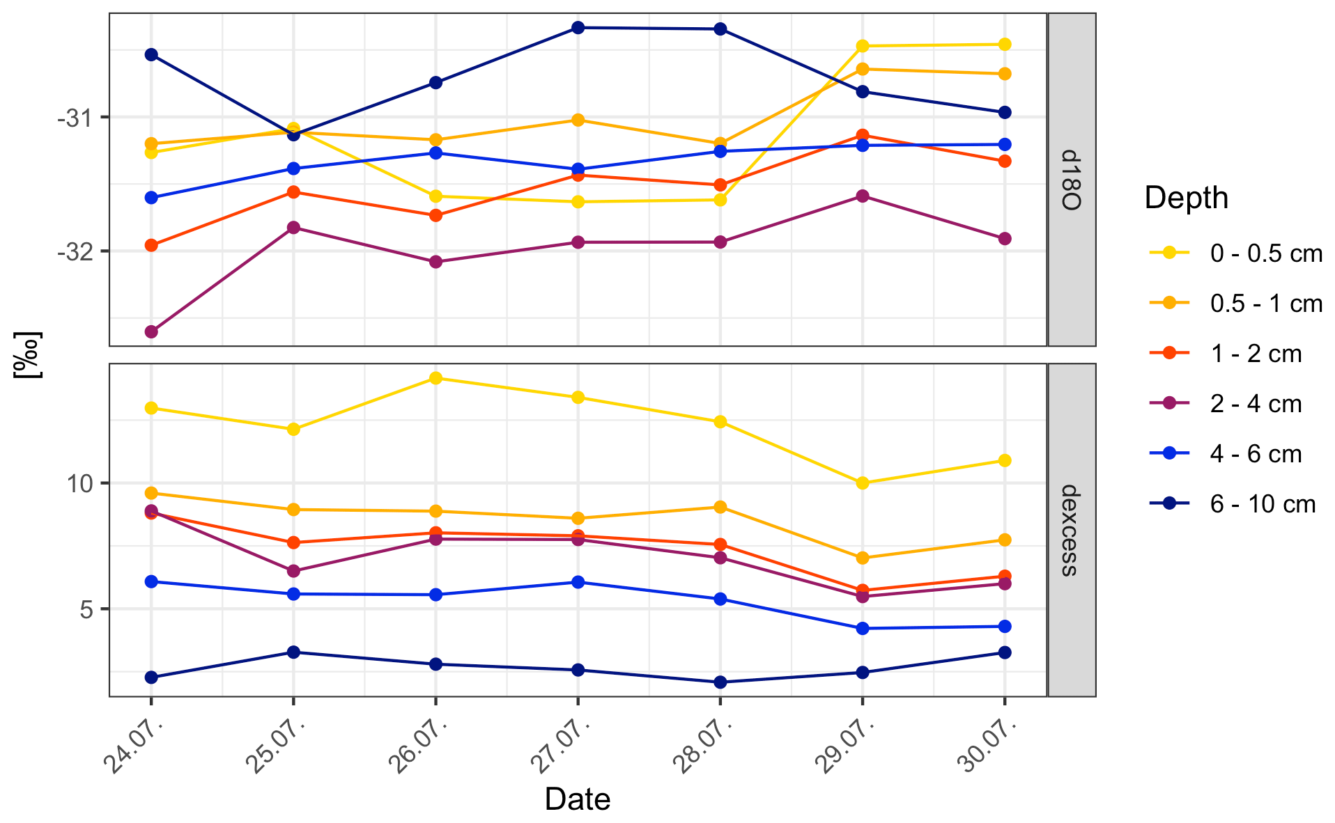
Figure 10 Spatial average δ¹⁸O and d-excess values during the second HIT period from 24 to 30 July 2018. The colour code indicates the sampled depth layer. Samples were taken at 25 positions in total: the first 10 with 1 m spacing, followed by 2 m spacing for the remaining 15 positions.

4 Discussion

This study presents δ¹⁸O and d-excess from the surface down to 10 cm depth at the EastGRIP camp site. These data can be used to study the evolution of the isotopic composition in the surface snow and upper snowpack to improve the understanding of the overall proxy signal formation and preservation stored in the isotopic composition. The data can further be used to investigate fluxes between the snow surface and the atmosphere as well as within the snowpack, e.g. via the implementation of fluxes and isotopes in models, such as MAR (e.g. Dietrich et al., 2024) and ECHAM-wiso (Cauquoin and Werner, 2021), and comparing these to these data. The outstanding characteristics of the presented dataset are the temporal sampling resolution, the spatial coverage (which averages out features from single locations) and the high vertical resolution.

4.1 Limitations of the dataset

The maximum sampled depth of 10 cm restricts the temporal coverage of the stable water isotope dataset to some months, depending on the accumulation conditions at each specific sampling site along the 39 m long transect. Hence, the data do not cover an entire seasonal cycle, impeding interpretations on a seasonal or annual scale. Moreover, with new snow accumulating over time, we cannot trace the temporal evolution of individual snow parcels. Nevertheless, based on the isotopic signature observed in the layers from 1–4 and 4–10 cm, we assume that the winter layer is apparent at some locations during the beginning of the observation period (δ¹⁸O values below −40 ‰, Fig. 5). We unfortunately cannot trace this layer at each location throughout the entire season, and hence this dataset does not allow conclusions on whether the winter layer persists within the snowpack or diffuses with time. Moreover, spatial variability introduced by moving the sampling position each time might cause additional uncertainty which should be considered when the aim is to analyse (near-)daily changes in the isotopic composition from nearby sampling locations.

The ability to combine this dataset with snow depth information from digital elevation models (DEMs) enables a variety of different analyses. However, DEMs are not available for each day of the observation period (14 May to 3 August 2018) and also not for each day of snow sampling (Table 1). This complicates the quantification of the contribution of snow accumulation and erosion to the observed isotopic signal. More information on the snowfall history, especially for the time preceding the sampling, with, for example, observations during the wintertime, and a deeper sampling might be beneficial to analyse year-round conditions of accumulation and (post-)depositional modifications of the isotope signature. Zuhr et al. (2023b) compare the internal structure and the δ¹⁸O composition of observed and simulated surface and subsurface snow over the summer period in 2019 (Fig. 6 in their publication), but they also lack detailed accumulation information prior to the sampling period. The available one-point measurements of snow height evolution at the nearby AWS can provide some information on the timing of large snowfall and erosion events (Zuhr et al., 2021b) but miss the spatial component.

4.2 Combining the stable water isotope data with other datasets

Recent studies performed at the EastGRIP site covered vapour fluxes and vapour–snow exchange processes (Hughes et al., 2021; Wahl et al., 2021, 2022), snow metamorphism (Harris Stuart et al., 2023), and snow height information to study local-scale snow deposition and redistribution (Zuhr et al., 2021b). Additional datasets for stable water isotopes for the summer season in 2018 are available covering two more transects (Fig. 1b; SSA transect: Steen-Larsen et al., 2022a; surface transect: Hörhold et al., 2022) as well as from continuous measurements of the isotopic composition in the water vapour (Steen-Larsen and Wahl, 2022).

4.2.1 Detailed snow height information

A photogrammetry structure-from-motion approach was performed during the same season in 2018 along the same transect as the presented data. The photogrammetry dataset from 2018 provides high-resolution near-daily digital elevation models (DEMs) with a horizontal resolution of 1 cm and sufficient accuracy for the purpose of the data presented here (RMSE of 1.3 cm, Zuhr et al., 2021b). The snow height is published in Zuhr et al. (2020) and Zuhr et al. (2021a). It is used to characterise spatio-temporal patterns of snow accumulation and erosion and offers insights into changes in surface structures (Zuhr et al., 2021b). The surface roughness decreased during the observation period with an overall flattening of the snow surface. Surface features, such as dunes and sastrugi, were more pronounced in May, showing a flattening of the surface and a decrease in surface roughness towards August 2018.

Combining DEM-derived snow height information and stable water isotope data can provide more insights into the buildup of the isotopic signal in the upper snowpack. Studies, such as Zuhr et al. (2023b), highlight the interoperability between the DEM-derived snow height information and isotope datasets. Zuhr et al. (2023b) demonstrate, for instance, that the temporal evolution of deeper layers shows the burying of older (more negative) snow with fresher (more enriched) snow, indicating that different processes influence the different depths within the upper snowpack. Considering the snow height evolution during the season in 2018 (bottom panel in Figs. 5 and 7) indicates that the observed changes in δ¹⁸O values in the layer of 4–10 cm (Fig. 5) are due to successive snow accumulation on the surface. Spatial accumulation variability can be derived from Zuhr et al. (2021b) and suggests that two dune features around 12 and 38 m along the transect at the beginning of the observation period coincide with low δ¹⁸O values, representing snowfall events and processes during previous seasons. Such characteristics are also observed in Zuhr et al. (2023b). However, DEM data are not available for every day of snow sampling in 2018 (Table 1), challenging a reliable assignment of individual snowfall events to specific layers throughout the season as well as individual height estimates of each sampling position. Nevertheless, the temporal sampling interval of 3 d or higher might reveal, together with available DEMs, insights into the near-daily evolution of the imprint and preservation of isotopic signatures as well as the influence of stratigraphic noise on these processes.

4.2.2 Additional stable water isotope data from the same area

A second snow sampling scheme, referred to as surface transect, was performed in the vicinity of the photogrammetry transect during the same time in 2018 (Fig. 1b). Snow was sampled daily in three depth intervals (0–0.5, 0–1 and 0–2 cm) at 11 positions with 10 m spacing along a 100 m transect. The samples were cumulatively stored in one bag per depth interval. Comparing these daily sampled data with the dataset presented in this study shows that the 3 d sampling captures the overall trend of the isotopic composition in the surface and subsurface snow (Fig. 11) but misses short-term fluctuations (e.g. between 30 July and 3 August). Moreover, snow–atmosphere surface exchange signals will be most visible in the thin 0–0.5 cm surface layer and already damped in the 0–1 cm layer. Some of the abrupt changes in δ¹⁸O are associated with large latent heat fluxes (e.g. after 4 June, Fig. 3), which could indicate sublimation-driven changes in isotopes. However, we also observed snowfall events (Fig. 3) that might dominate the surface and subsurface snow layers and their isotopic composition, especially if the amount of snowfall was larger than the sampled layer. Deciphering the individual contributions to the overall isotopic signal requires a more in-depth analysis and would benefit from more information, such as amount of snowfall and strength of snow redistribution.

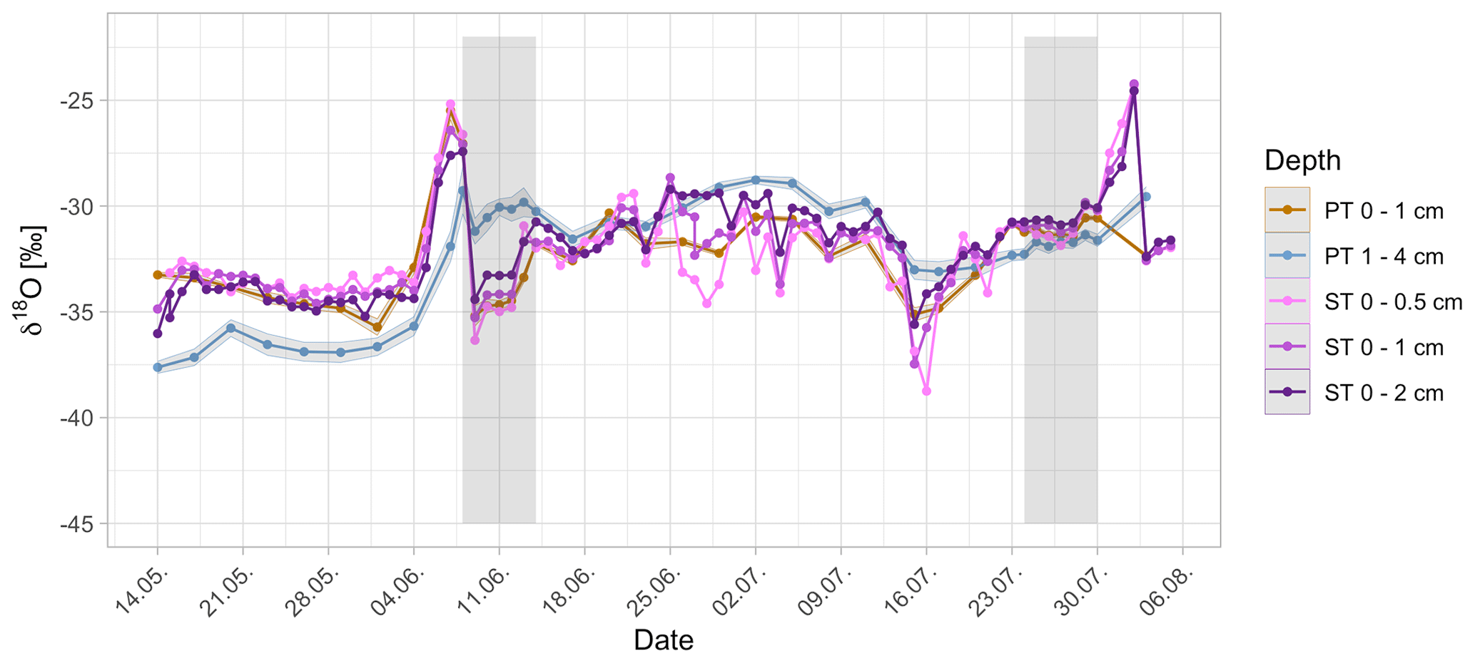
Figure 11 Comparison of δ¹⁸O data from this study (PT; first and second layer, averaged per day and depth interval with respective standard error) and the consolidated samples from the surface transect (ST), all from the year 2018. The location of the surface transect is shown in Fig. 1b.

At the same study site, Zuhr et al. (2023b) sampled the top 30 cm of the snowpack with a vertical resolution of 2 cm along a 40 m long transect (Fig. 1b and c in their study) between 27 May and 27 July 2019. Instead of high temporal resolution as in this study, their study sampled the upper 30 cm with higher vertical resolution, but only six times. Their isotope dataset is accompanied by near-daily DEMs. The deeper sampling provides insights into the internal layering of the isotopic composition as well as the temporal evolution of these layers. During the 2019 season, Zuhr et al. (2023b) recorded only 13 snowfall events (Fig. 2b in their study), while the season in 2018 had 29 documented snowfall events (Fig. 3). This suggests that the isotopic composition in 2018 might be more influenced by a snowfall-driven signal, while their dataset from 2019 could reveal a signal formed by atmosphere–snow exchange processes, as discussed in their study. More in-depth analyses of the DEMs and other data that indicate timing and amount of snowfall might provide a deeper understanding of the observed changes in δ¹⁸O in the upper snowpack during a snowfall-dominated season.

4.2.3 Information on atmosphere–snow exchange processes

Besides physical modifications of the snow surface by snow erosion and redistribution (Zuhr et al., 2021b), vapour–snow exchange processes contribute to the surface snow isotope variability (e.g. Casado et al., 2021; Hughes et al., 2021; Wahl et al., 2022; Harris Stuart et al., 2023). The presented dataset is suitable to study these exchange processes by combining detailed isotope measurements with other information and datasets. Studies with a focus on isotope and humidity fluxes have already shown that if the conditions for isotopic exchange between the atmospheric water vapour and the snow surface are given, especially in snowfall-free periods, a post-depositional atmospheric signal is introduced into the surface layer (Wahl et al., 2022). Isotope and humidity fluxes are, for instance, available from the same study site and season (Steen-Larsen and Wahl, 2022; Steen-Larsen et al., 2022b) as well as from the nearby AWS. The large increase in temperature after 4 June is accompanied by a high latent heat flux (LE) (Figs. 2 and 6). Both could contribute to a sublimation-driven increase in δ¹⁸O. However, we also observed snowfall between 5 and 9 June (Fig. 2), which might dominate the isotopic composition of the surface snow and upper snowpack. Additional evidence for fractionation effects during sublimation (Madsen et al., 2019; Wahl et al., 2021) and vapour diffusion within the snowpack (snow metamorphism) is reported in a study that analysed SSA and isotope data at the EastGRIP campsite for several years between 2016 and 2019 (Harris Stuart et al., 2023). A detailed analysis of isotopic variability from the presented dataset in conjunction with SSA changes (Steen-Larsen et al., 2022a) can help quantify the different contributions of snowfall, redistribution and vapour–snow exchange to the obtained isotope signal in the upper snowpack.

5 Data availability

All isotope data are available on PANGAEA via https://doi.org/10.1594/PANGAEA.956626 (Zuhr et al., 2023a). This dataset includes the variables δ¹⁸O, δD and d-excess as well as their respective standard deviation based on the measurement. The data are labelled with their respective location along the transect and the depth of sampling as well as the date of sampling (date, time and day of year in 2018).

6 Conclusions

We present stable water isotope data with high temporal and spatial resolution from samples taken next to the EastGRIP campsite in northeast Greenland for the summer season in 2018. The spatio-temporal variability suggests that snow erosion and drift contribute considerably to the observed isotopic composition. The consideration of additional processes, such as vapour–snow exchange, might be necessary to capture the influence of (post-)depositional modifications on the proxy signal formation and preservation within the upper snowpack. The location of the EastGRIP campsite in the accumulation zone of the Greenland ice sheet is very suitable for such investigations due to the absence of melt during the summer and a sufficiently high accumulation rate to show seasonal layering. More analyses, for instance, combining these data with complementary datasets, e.g. snow height information and vapour flux measurements, will contribute to an improved understanding of the climatic signal contained in stable water isotopes in firn and ice cores.