A synthesis of Global Streamflow Characteristics, Hydrometeorology, and Catchment Attributes (GSHA) for large sample river-centric studies

Our understanding and predictive capability of streamflow processes largely rely on high-quality datasets that depict a river's upstream basin characteristics. Recent proliferation of large sample hydrology (LSH) datasets has promoted model parameter estimation and data-driven analyses of hydrological processes worldwide, yet existing LSH is still insufficient in terms of sample coverage, uncertainty estimates, and dynamic descriptions of anthropogenic activities. To bridge the gap, we contribute the synthesis of Global Streamflow characteristics, Hydrometeorology, and catchment Attributes (GSHA) to complement existing LSH datasets, which covers 21 568 watersheds from 13 agencies for as long as 43 years based on discharge observations scraped from the internet. In addition to annual and monthly streamflow indices, each basin's daily meteorological variables (i.e., precipitation, 2 m air temperature, longwave/shortwave radiation, wind speed, actual and potential evapotranspiration), daily–weekly water storage terms (i.e., snow water equivalence, soil moisture, groundwater percentage), and yearly dynamic descriptors of the land surface characteristics (i.e., urban/cropland/forest fractions, leaf area index, reservoir storage and degree of regulation) are also provided by combining openly available remote sensing and reanalysis datasets. The uncertainties in all meteorological variables are estimated with independent data sources. Our analyses reveal the following insights: (i) the meteorological data uncertainties vary across variables and geographical regions, and the revealed pattern should be accounted for by LSH users; (ii) ∼6 % watersheds shifted between human-managed and natural states during 2001–2015, e.g., basins with environmental recovery projects in northeast China, which may be useful for hydrologic analysis that takes the changing land surface characteristics into account; and (iii) GSHA watersheds showed a more widespread declining trend in runoff coefficient than an increasing trend, pointing towards critical water availability issues. Overall, GSHA is expected to serve hydrological model parameter estimation and data-driven analyses as it continues to improve. GSHA v1.1 can be accessed at https://doi.org/10.5281/zenodo.8090704 and https://doi.org/10.5281/zenodo.10433905 (Yin et al., 2023a, b).

1 Introduction

Climate change has posed profound challenges to the management of freshwater resources, specifically riverine floods and water shortages (AghaKouchak et al., 2020; Thackeray et al., 2022). The urgent need for flood and drought forecasting and water resources planning and management calls for high-quality streamflow predictions for basins worldwide to analyze global terrestrial water conditions from a systematic view (Burges, 1998). The scarcity of hydrological observations has brought challenges to these predictions (Belvederesi et al., 2022; Hrachowitz et al., 2013); thus, the development of computer models that allow for “modelling everything everywhere” (Beven and Alcock, 2012) constitutes the backbone of hydrological studies. Existing studies have used physically based and data-driven models for streamflow simulation (Lin et al., 2018; Nandi and Reddy, 2022; Zhang et al., 2020), with efforts to improve accuracy of prediction by combining them (Cho and Kim, 2022; Razavi and Coulibaly, 2013). Yet the prediction of the magnitude, timing, and trend of critical streamflow characteristics are still subject to multiple sources of errors and uncertainties (Bourdin et al., 2012; Brunner et al., 2021).

Streamflow (Q) can be represented by the simple water balance equation involving precipitation (P), evapotranspiration (ET), and water storage terms (S) denoted as $Q=P-\text{ET}-\mathrm{\Delta }S$, yet influencing factors of these components could bring uncertainties that cascade downstream. Starting from the model assumptions to the data used to represent climate, soil water, ice cover, topography, and land use, as well as the less well-known processes such as human perturbations and sub-surface flows (Benke et al., 2008; Wilby and Dessai, 2010), these complications impede our understanding of streamflow processes across scales, which also limits the streamflow modeling and predictive capability. Thus, reducing the predictive uncertainties requires high-quality data with numerous samples capable of depicting each of the water balance components and the natural and anthropogenic factors involved (Gupta et al., 2014).

Efforts have been made to address the need for such high-quality datasets on watershed-scale hydro-climate and environmental conditions during the past couple of decades. One of the earliest was the most widely used dataset generated for the Model Parameter Estimation Experiment (MOPEX) project aimed at better hydrological modeling (Duan et al., 2006). Historical hydro-meteorological data and land surface characteristics for over 400 hydrologic basins in the United States were provided and are fundamental to the progress in large sample hydrology (LSH) (Addor et al., 2020; Schaake et al., 2006). Later the dataset was expanded to 671 catchments in the contiguous United States (CONUS) and benchmarked by model results (Newman et al., 2015). Based on these studies, the Catchment Attributes and Meteorology for Large-sample Studies (CAMELS) dataset was developed, providing comprehensive and updated data on topography, climate, streamflow, land cover, soil, and geology attributes for each catchment (Addor et al., 2017). The CONUS CAMELS dataset soon became influential in LSH and has since inspired researchers from Australia (Fowler et al., 2021), Europe (Coxon et al., 2020; Delaigue et al., 2022; Klingler et al., 2021), South America (Alvarez-Garreton et al., 2018; Chagas et al., 2020), and China (Hao et al., 2021) to contribute their regional CAMELS. Another comprehensive regional LSH dataset for North America named the Hydrometeorological Sandbox – École de Technologies Supérieure (HYSETS) dataset was also developed with larger sample size (14 425 watersheds) and richer data sources compared with the CAMELS (Arsenault et al., 2020).

While these datasets are reliable data sources for regional studies, attempts at building global datasets have become the new norm in the era of big data to boost our analytical and modeling capability for the terrestrial hydrological processes. The HydroATLAS dataset integrated indices of hydrology, physiography, climate, land cover, soil, geology, and anthropogenic activity attributes for 8.5 million global river reaches (Lehner et al., 2022; Linke et al., 2019). A recent work combined a series of CAMELS datasets with HydroATLAS attributes into a new global community dataset in the cloud named Caravan, with dynamic hydro-climate variables and comprehensive static catchment attributes extracted on 6830 watersheds (Kratzert et al., 2023), which represents by far the most comprehensive synthesis of existing CAMELS. Another global-scale effort, the Global Streamflow Indices and Metadata archive (GSIM), incorporated dynamic streamflow indices and attribute metadata for topography, climate type, land cover, etc., for over 35 000 gauges (Do et al., 2018; Gudmundsson et al., 2018), and the streamflow indices were updated to allow for trend analysis (Chen et al., 2023). A recent study filled in the discontinuity and latency of gauge records and provided streamflow for over 45 000 gauges with improved data quality (Riggs et al., 2023). These global-scale datasets have been widely used in data-driven machine learning models (Kratzert et al., 2019; Ren et al., 2020), physical hydrological models (Aerts et al., 2022; Clark et al., 2021), and parameter estimation and regionalization studies (Addor et al., 2018; Fang et al., 2022).

Although the flourishing of LSH datasets has promoted comparative hydrological studies (Kovács, 1984) and large-scale hydrological modeling and analysis efforts, several challenges still stand in the way of realizing the full potential of LSH. As briefly outlined in a recent review by Addor et al. (2020), current LSH datasets lack common standards, metadata, and uncertainty estimates and are insufficient at characterizing human interventions. More specifically, the following major critical aspects still need attention from the LSH developers, which we attempt to address with the synthesis of Global Streamflow characteristics, Hydrometeorology, and catchment Attributes (GSHA) (Yin et al., 2023a, b). First, the majority of current datasets (especially those at a global scale) incorporated only one data source for each variable, while Earth observations, reanalysis, and satellite-based estimates are subject to uncertainties (Merchant et al., 2017; Ukhurebor et al., 2020). These uncertainties have rarely been represented and may present difficulties in the regionalization of model parameters (Beck et al., 2016) while also resulting in inconsistent conclusions. Second, anthropogenic activities including land use and land cover (LULC) changes, dam and reservoir building, etc., are critical drivers of shifts in streamflow statistical moments (Niraula et al., 2015). However, historical time series of watershed human modifications have rarely been included in LSH datasets, which is particularly problematic for regions with rapid economic growth. Finally, although the most recent Caravan provided hydroclimate data for global watersheds, the samples are limited to the existing regional CAMELS that Caravan synthesizes. Therefore, plenty of room is left to increase data sample size and spatial coverage by revisiting the streamflow data acquisition process in a more comprehensive way.

To complement existing LSH datasets, we contribute the first version of a synthesis of Global Streamflow characteristics, Hydrometeorology, and catchment Attributes (GSHA v_1.0) for large-sample river-centric studies. GSHA features the following characteristics:

• updated physical and anthropogenic descriptors of global rivers, covering streamflow characteristics, hydrometeorological variables, and land use land cover changes for 21 568 watersheds derived from gauged streamflow records from 13 agencies;

• streamflow indices for data scarce regions, including those derived from 263 gauges in China;

• extended temporal coverage for as long as 43 years (1979–2021), which varies regionally;

• uncertainty estimates for the meteorological variables; and

• dynamic descriptors for the urban, forest, and cropland fractions, as well as reservoir storage capacity to improve the representation of human activities in the basin.

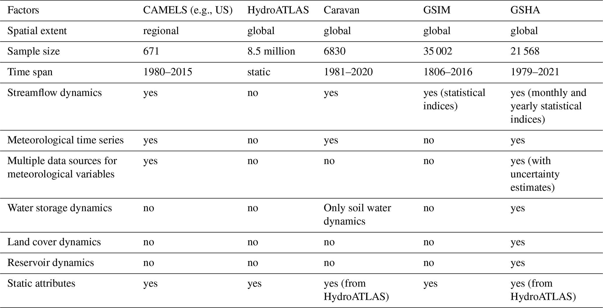
With the above features, we expect GSHA to support hydrological model parameter estimation and data-driven analysis of global streamflow as one of the most comprehensive LSH datasets regarding sample size, variable dynamics, and uncertainty estimates. Table 1 summarizes the differences between GSHA and other prominent LSH datasets. Our paper is organized as follows. Section 2 expands on Table 1 and provides more details of the data included for GSHA. Section 3 introduces the data sources and methodologies involved in creating GSHA. Section 4 highlights the key features of GSHA by conducting some analyses, followed by conclusions reached in Sect. 5.

Table 1 Comparison of GSHA with other LSH datasets. Note that we only include the CONUS CAMELS dataset to represent regional LSH datasets for this comparison, as other regional CAMELS share large similarity with CONUS CAMELS.

2 Dataset content of GSHA v1

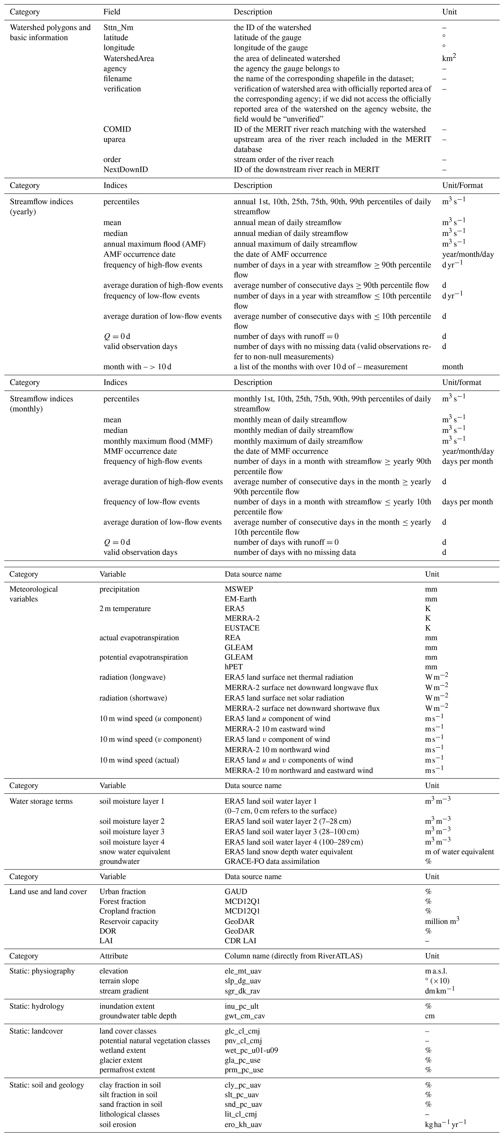
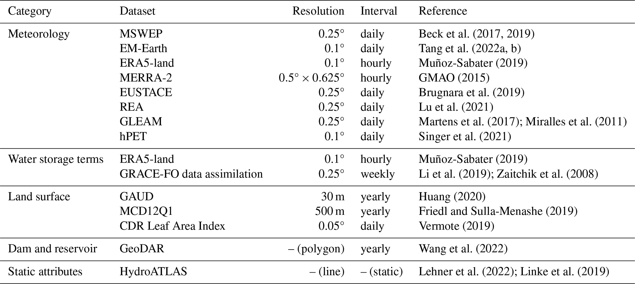
In this section, the data fields, variables, and attributes included in GSHA are described in more details and summarized in Table 2. For the instructions of the data format, we provide a user manual along with the dataset (see Yin et al., 2023b). GSHA includes yearly and monthly streamflow characteristics derived from daily discharge observations, meteorological variables (including precipitation, 2 m air temperature, longwave and shortwave radiation, wind speed, and actual and potential evapotranspiration (AET and PET)), daily or weekly water storage terms (four layers of soil moisture, groundwater, and snow depth water equivalence), daily vegetation index (leaf area index (LAI)), yearly LULC characteristics (urban, cropland, and forest fraction), and yearly reservoir information (degree of regulation (DOR) and reservoir capacity). For each meteorological variable, multiple independent data sources are incorporated to provide uncertainty estimates. Static attributes like land physiography, soils, and geology are not additionally extracted, as similar efforts have been made by other researchers, so we directly matched our gauge locations to the HydroATLAS dataset (Lehner et al., 2022; Linke et al., 2019) by providing the river ID match table. Users can link the two to obtain these attributes.

• Watershed polygons: GSHA includes 21 568 watershed polygons delineated from the global gauges, which are stored in ESRI shapefile format. The ID and agency of each watershed are the same as the corresponding gauge ID, and the gauge latitude/longitude are in decimal degree. The area denotes the upstream drainage area of the gauge. Some of the IDs contain characters (such as “.” or “-”) inconsistent with the majority of IDs. For the convenience of the users, we unified these as underscores and stored the new file names as “filename”. We also provide independent files summarizing basic information of the watersheds, including matched MERIT river reach COMID (the identification field for each river reach), upstream area, order and downstream river reach COMID, and verification with officially reported areas of the agencies.

• Streamflow indices: GSHA publishes annual and monthly streamflow indices derived from daily streamflow data, including different percentiles and mean/median/minimum/maximum. The frequency and durations of extremely high and low streamflow events are also provided. We also include numbers of zero observations and valid samples to allow flexible data screening by the users. The indices are stored as comma-separated values (CSV) files, with each watershed corresponding to one file. A complementary R package can be used to automatically download many of the gauge datasets, available at https://github.com/Ryan-Riggs/RivRetrieve (last access: 26 July 2023) (Riggs et al., 2023).

• Meteorological variables: The meteorological variables selected are the most influential drivers for streamflow and include precipitation, 2 m temperature, ET, radiation, and wind speed. In mainstream land surface models, ET is a diagnostic variable derived from meteorological inputs and is not considered meteorological forcing. However, as many hydrological models also use potential ET as an input variable, and model calibration sometimes involves actual ET (Immerzeel and Droogers, 2008), we include the two variables and place them into the meteorological variable category. For each variable, multiple data sources are used to allow for uncertainty analysis, which is provided on a yearly basis in an independent file.

• Natural water storage terms and land use/land cover change: These include soil moisture, snow water equivalent, and groundwater percentages. We also include yearly land cover dynamics (i.e., urban, forest, and cropland fraction changes) as well as dynamically changing reservoir capacity and degree of regulation (DOR) percentage. Leaf area index (LAI) is also included to reflect the seasonal changes in vegetation canopy that are also key to the streamflow processes.

• Static attributes: GSHA does not extract updated static attributes because HydroATLAS already made substantial efforts in this regard. Instead, the listed categories are those mostly related to streamflow prediction from HydroATLAS selected to be included in GSHA files, and we direct the readers to the ID match table to access the entire 281 static attributes offered by HydroATLAS (Lehner et al., 2022; Linke et al., 2019). Our user manual, available at the dataset download site, also provides more information on it.

Table 2 Fields provided with GSHA.

3 Data sources and methodology

3.1 Technical workflow in creating GSHA

The creation of GSHA starts from revisiting the data compilation process for the stream gauging observations from 13 international agencies. The general workflow of GSHA data production processes is illustrated in Fig. 1, which consists of watershed delineation, variable extraction from both grid and non-grid data sources, and uncertainty analysis.

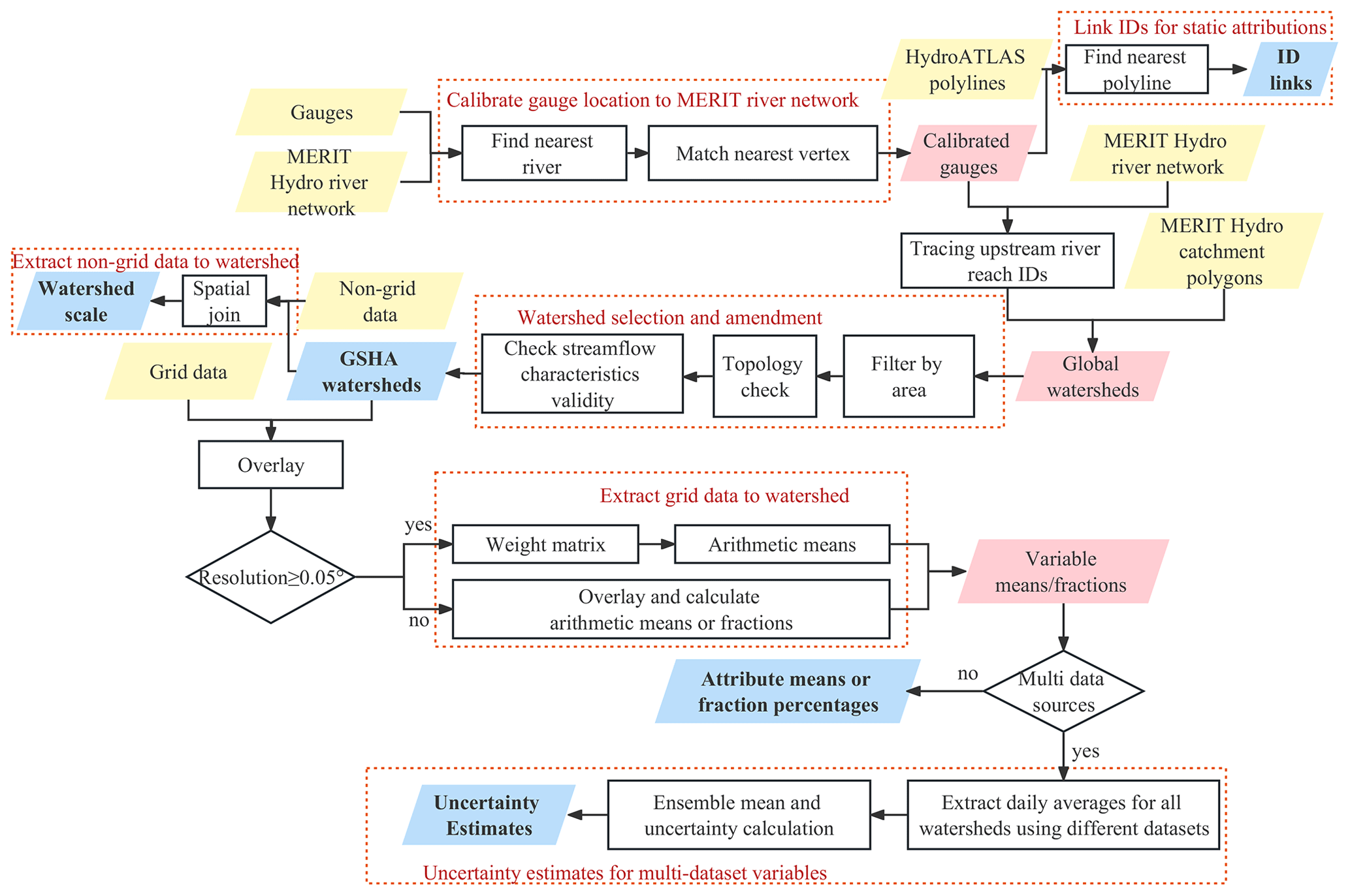
Figure 1 General workflow of GSHA. The yellow parallelograms are the input datasets, the blue ones are the final outputs of GSHA dataset, and the pink ones are the results in the process. The black quadrilaterals represent the extraction and calculation processes, and the dotted red rectangles illustrate different modules of the extraction process.

First, we delineated the upstream watersheds using gauge locations. Calibration of gauge longitudes and latitudes were conducted to match the gauges with the MERIT river network exactly. The delineated watersheds were selected and manually checked using standards of area, topology correctness, and observation data lengths. The selected watersheds went on to be overlaid with grid and non-grid variable data sources to obtain GSHA variables.

3.2 Gauge-based streamflow indices

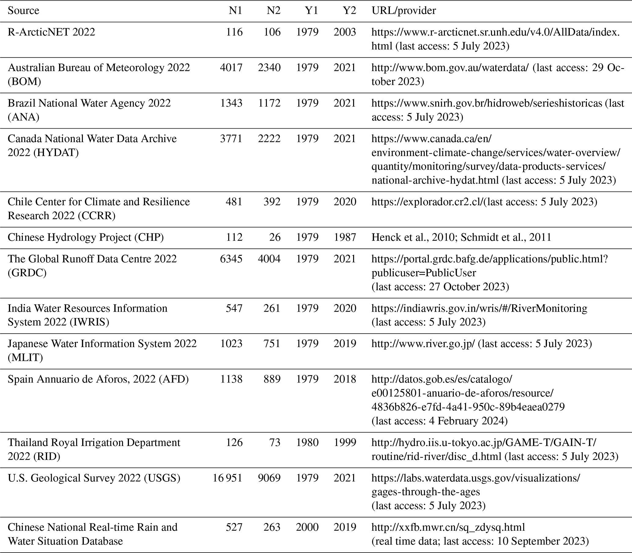
As shown in Table 3, in total streamflow data from 36 497 gauges were initially scraped from the web and from the Chinese National Real-time Rain and Water Situation Database. For gauges located within ∼100 m of each other, those with fewer years of measurements were removed, assuming that they are redundant with one another. The gauge measurements were converted to a consistent unit (m³ s⁻¹) and then manually compared with Global Runoff Data Centre (GRDC) measurements to ensure accurate unit conversion (Riggs et al., 2023). Gauge databases compiled in this study are available through a variety of web interfaces, except for the Chinese Hydrology Project (CHP) data, which are provided by the authors of the dataset (Henck et al., 2010; Schmidt et al., 2011), and processed into annual-scale data that meet the requirements of the synthesis dataset.

Table 3 Gauge data sources used in this analysis. N1 and N2 refer to numbers of gauges with observations after 1979 and used in GSHA. The starting and ending years (Y1 and Y2) of GSHA gauges for each agency are listed.

3.3 Watershed delineation

The watershed delineation process was built upon a vector-based global river network dataset (Lin et al., 2021), which is delineated from the 90 m Multi-Error-Removed Improved Terrain (MERIT) digital elevation model (DEM) (Yamazaki et al., 2017) and the flow direction and flow accumulation rasters (Yamazaki et al., 2019). The locations of the gauges may contain locational errors and direct delineation will result into erroneous watershed boundaries; therefore, gauge location correction was conducted by relocating the gauges to the nearest MERIT-based river reach vertices. The adjusted gauge points were used as the watershed outlets, where the contributing areas were extracted by dissolving all upstream catchments based on the topology provided by MERIT-Basins (Lin et al., 2019). Since the area threshold of MERIT-Basins is 25 km², we did not include watersheds smaller than this threshold. Considering the spatial heterogeneity of very large basins, we excluded watersheds ≥50 000 km² from the dataset. To ensure GSHA supports studies with sufficiently long records, only watersheds with >5 years of observations since 1979 were selected. For gauges sharing the same watershed, the one with better data quality (i.e., longer measurement records and more valid observation days) was used. If the two gauges share the same quality, we only included the furthest downstream gauge. Eventually, the selection processes resulted in 21 568 valid watersheds out of 35 970 gauges initially scraped from the web plus 527 gauges from the Chinese National Real-time Rain and Water Situation Database (Fig. 2).

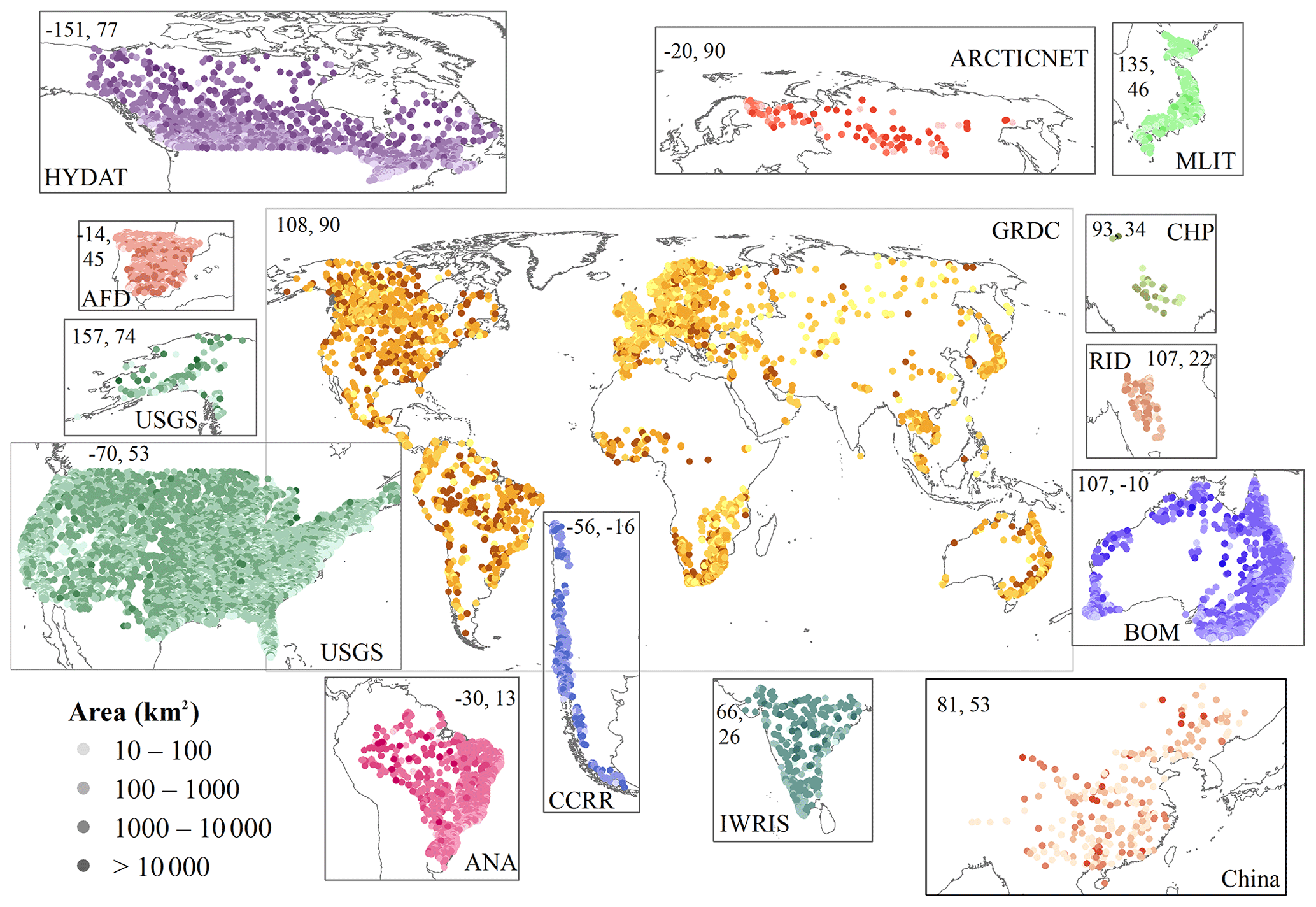
Figure 2 Spatial distribution of the GSHA gauges (n=21 568). Watershed area size is represented by the color shading. Gauges of different agencies are represented with separate colors and are plotted in individual frames (except for USGS gauges in two frames to incorporate Alaska). The agency names and longitude and latitude coordinates (in °) of each frame are also shown in the figure.

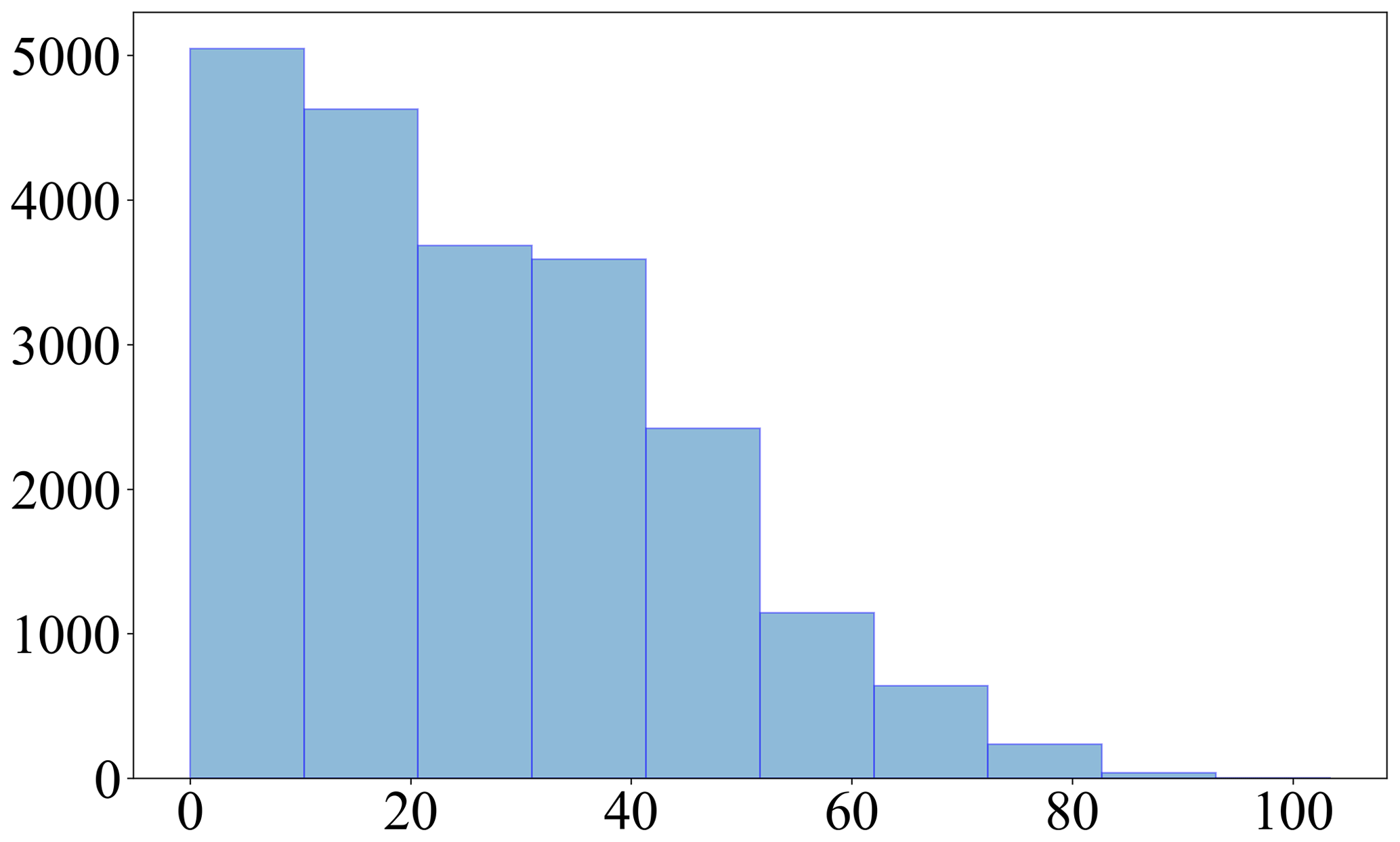
The GSHA watersheds are unevenly distributed across the globe, more than half of which are located in North America (USGS, HYDAT, and a large proportion of GRDC gauges, Fig. 3a). Europe, Australia, and South America also have relatively good coverage, while Asia and Africa show the lowest gauge densities. The majority of the gauged watersheds are of medium sizes ranging from 250 to 2500 km², although for some agencies it does not show the same distribution (Fig. 3d). For instance, ANA (South America), IWRIS (India), and ArcticNet (northern Eurasia) watersheds are generally larger, while the Chinese National Real-time Rain and Water Situation Database provides more gauges with smaller drainage areas. Due to the maintenance difficulties, the number of functioning gauges is declining for agencies like GRDC, but the lack of data in recent years (Fig. 3c) is mainly due to latency issues. USGS, BOM, and ANA provide a stable number of observations for the 1980–2021 period (Fig. 3c) with high proportions of valid observations each year (Fig. 3b), while observational periods from ArcticNet and China contain relatively fewer valid samples (Fig. 3b) and shorter time spans (Fig. 3c).

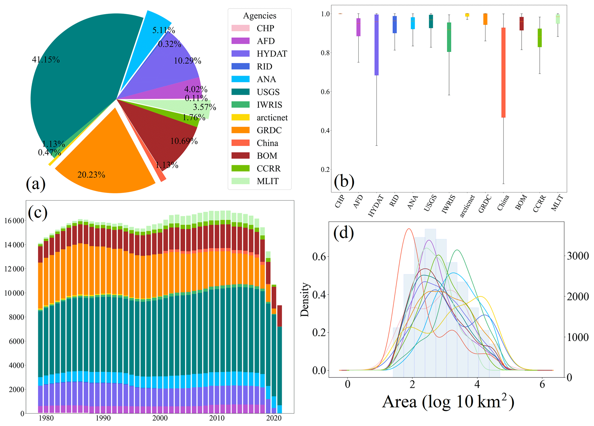
Figure 3 Summary statistics of the GSHA gauges. This includes (a) proportions of gauges from different agencies, (b) box plots of proportions of valid observations for each agency, (c) proportion of valid observation for each year by agency, and (d) distributions of watershed areas for each agency (kernel density estimation lines, left y axis) and all gauges (blue histogram, right y axis). The color legend in panel (a) applies to all four panels. In panel (a) the 0.11 % label corresponds to CHP, and the legend goes counter clockwise in the pie chart. In panel (c), CHP bars are at the bottom of the plot, and the legend goes from bottom to the top of the bars.

3.4 Meteorological variables, water storage terms, and land surface characteristics

After watershed delineation, publicly available grid or non-grid data were obtained and overlaid to derive the meteorological, water storage terms, and land surface characteristics. The data sources used for GSHA are listed in Table 4. We prioritized the use of multi-source fusion datasets with relatively high quality surveyed from literature when creating GSHA.

Table 4 Data sources used for the GSHA variables.

3.4.1 Meteorology datasets

For precipitation, the Multi-Source Weighted-Ensemble Precipitation (MSWEP) that merged gauge measurements (CPC Unified), grid data (GPCC), satellite products (CMORPH, GSMaP-MVK, and TMPA 3B42RT), and reanalysis data (ERA-Interim and JRA-55), with sample density and comparative performance considered (Beck et al., 2017, 2019), are included. Another precipitation dataset is the Ensemble Meteorological Dataset for Planet Earth (EM-Earth) deterministic estimates, which merged the station-based serially complete Earth dataset (SC-Earth) removing the temporal discontinuities in raw station observations and ERA5 estimates (Tang et al., 2022b).

For 2 m air temperature, the EUSTACE global land station daily air temperature dataset, which statistically merged station and satellite observations to obtain global daily near-surface air temperature (Brugnara et al., 2019), is included. Other datasets used for 2 m temperature extraction are the reanalysis datasets Modern-Era Retrospective analysis for Research and Applications Version 2 (MERRA-2) (Gelaro et al., 2017) and the fifth generation of European Reanalysis (ERA5) dataset land component (Muñoz-Sabater et al., 2021). MERRA-2, produced by NASA's Global Modeling and Assimilation Office (GMAO), used the Goddard Earth Observing System (GEOS) model and analysis scheme and assimilated the latest observations. ERA5 reanalysis was developed by the European Centre for Medium-Range Weather Forecasts (ECMWF) using the Carbon Hydrology-Tiled ECMWF Scheme for Surface Exchanges over Land (CHTESSEL) driven by the downscaled meteorological forcing from the ERA5 climate reanalysis (Hersbach et al., 2020). These reanalysis datasets are also used in extracting longwave and shortwave radiation, as well as u and v components of wind.

For AET, the REA dataset, which used the reliability ensemble averaging (REA) method to merge ERA5, Global Land Data Assimilation System Version 2 (GLDAS2), and MERRA-2, is used (Lu et al., 2021). Another AET data source is the product of the Global Land Evaporation Amsterdam Model (GLEAM) based on satellite observations of surface net radiation and near-surface air temperature (Martens et al., 2017). For PET, GLEAM is also incorporated. Another PET dataset for GSHA is an hourly PET at 0.1° resolution for the global land surface (hPET) calculated from ERA5-land wind speed, air and dew point temperature, net radiation components, and surface air pressure (Singer et al., 2021).

3.4.2 Water storage term datasets

ERA5-land data are also applied in extracting soil moisture for four soil layers as well as snow water equivalence. For groundwater, an assimilation dataset from NASA's Gravity Recovery and Climate Experiment (GRACE) and its follow-on mission (GRACE-FO) is used (Li et al., 2019). The dataset merged water storage derived from GRACE satellite products into ECMWF Integrated Forecasting System meteorological data-forced NASA's Catchment land surface model (CLSM). The data are represented as groundwater drought indicator (GWI), which is the percentage of groundwater storage estimates from the GRACE data assimilation relative to the climatology (representing historical conditions), at weekly timescales from 2003 to 2021.

3.4.3 Land surface characteristic datasets

Global urban development for 1985–2015 is represented as the urban fraction in each watershed using the global annual urban dynamics (GAUD) at 30 m resolution. The dataset was derived from Landsat surface reflectance based on the Normalized Urban Areas Composite Index (NUACI) (Liu et al., 2020). For forest and cropland fractions, the Terra and Aqua combined Moderate Resolution Imaging Spectroradiometer (MODIS) Land Cover Type (MCD12Q1) land cover dataset is used (Friedl et al., 2010). It covers 2001–2020 with a resolution of 500 m, and the categories used for GSHA are the International Geosphere–Biosphere Programme classification (IGBP) forests and croplands. Another land cover is vegetation, which is represented by LAI obtained from the National Oceanic and Atmospheric Administration (NOAA) Climate Data Record (CDR) of Advanced Very High-Resolution Radiometer (AVHRR) product, which relied on artificial neural networks and the AVH09C1 surface reflectance product (Claverie et al., 2016).

3.4.4 Dams and reservoirs

The newly published Georeferenced global Dams And Reservoirs (GeoDAR) dataset that documented the dam and reservoir construction years is used for building the temporally varying watershed reservoir capacity and DOR. GeoDAR georeferenced the International Commission on Large Dams (ICOLD) World Register of Dams (WRD) and geo-matched multi-source regional registers and geocoding descriptive attributes through the Google Maps API (Wang et al., 2022). The reservoir capacities are used together with the mean annual streamflow to obtain the DOR based on equation $\text{dor}=\text{SC}/Q_{\text{mean}}$, where SC refers to reservoir storage capacity and Q_mean is the mean annual streamflow in the corresponding year.

3.4.5 Static variables

We matched GSHA river IDs and HydroATLAS river reach IDs to link the static attributes. HydroATLAS includes 56 variables for hydrology, physiography, climate, land cover and use, soils and geology, and anthropogenic influences for over 8.5 million river reaches globally.

3.5 Variable extraction methods

For grid data with relatively coarse spatial resolutions (≥0.05°), we used an area-weighted approach to extract the variable (Addor et al., 2017) based on the proportion of the grid area contained in the basin boundary, while for high-resolution grid data, we extracted the arithmetic mean directly. Figure 4 shows the area-weighted average approach we used for grid data with spatial resolution ≥0.05° to reduce the influence of watershed area on data uncertainty (Tang et al., 2023). The grid data (Fig. 4a) and the quality-controlled watersheds (Fig. 4b) were overlaid and all grids intersecting with the watershed were obtained (Fig. 4c). For each intersected grid, the proportion of the polygon in the grid was calculated as the weight (dark blue, Fig. 4d); the product of the weight and the corresponding grid value was calculated over all intersected grids (Fig. 4e) and was summed up as the weighted average (Fig. 4f). For wind, the u and v wind components were first used to calculate wind speed, then the basin average was calculated with the weighted average approach. For grid data with a spatial resolution of <0.05°, the area-weighted approach was not adopted as it offers limited gains while becoming computationally too expensive. For reservoirs, we used the reservoir polygons in GeoDAR, which were spatially joined to GSHA watershed polygons. All the intersected reservoirs were considered contributory to the management of the corresponding watershed and were used to calculate the total reservoir storage capacity and degree of regulation.

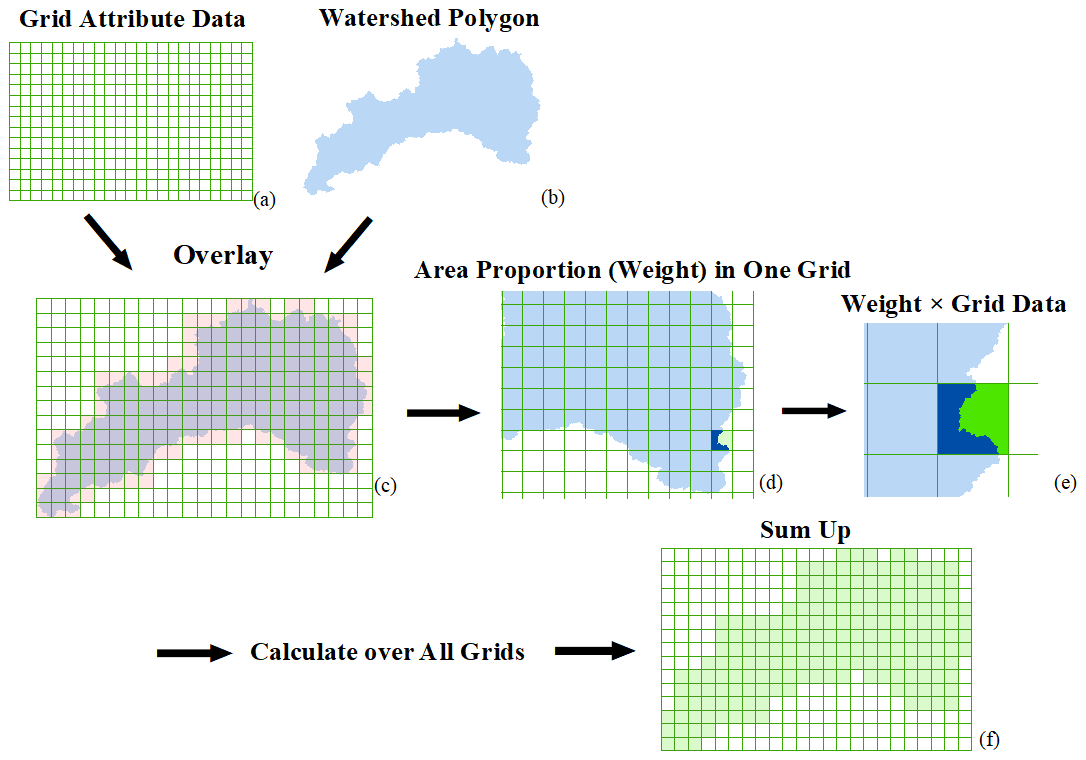
Figure 4 Determination of the area weights in extracting gridded data to GSHA watershed polygons. This weighted approach is applied to data at a resolution of ≥0.05° but not for data at a finer spatial resolution due to computational costs.

3.6 Uncertainty estimates

We also provided uncertainty estimates of the meteorological variables by calculating the long-term mean of each dataset in each watershed, where the discrepancy between the maximum and minimum among the data sources (X_max and X_min) as a percentage of their mean ($\stackrel{\mathrm{‾}}{X}$) was used in the uncertainty estimation:

$$\begin{array}{}\text{(1)}& \text{uncertainty}={\displaystyle \frac{X_{\text{max}}-X_{\text{min}}}{\stackrel{\mathrm{‾}}{X}}}\cdot \mathrm{100}\mathit{\%}.\end{array}$$

3.7 Validation

After delineation, we validated our watershed areas with officially reported watershed areas from BOM, HYDAT, and GRDC by matching GSHA watersheds by their agency IDs. We set the criteria of mismatched watersheds as (1) the area difference being greater than ±20 % of the officially reported area and (2) the area ratio being less than 0.1 or greater than 10 times the reported areas. Since not all agency websites reported watershed areas, thus we added a flag field in the attributes with “unverified”, “verified match”, and “verified mismatch” to allow users to filter the watersheds flexibly and avoid putting the samples in the dataset under an inconsistent standard.

Postprocessing of the extracted variables includes the unification of units and manual quality checks. For streamflow characteristics, we validated three of our indices against GSIM for its global coverage, including the mean annual streamflow and 10th and 90th percentiles. The spatial joint between GSHA and GSIM gauges in a 10 km buffer zone was performed, and only GSIM gauges with a minimum distance and watershed area difference ≤5 % to a GSHA gauge were considered. Pairs with zero measurements were excluded and 9835 pairs were included eventually. We plotted the scatterplot of GSHA-GSIM mean flow, and 10th and 90th percentiles, and compared the fitting line to the 1:1 line, with correlation coefficients calculated (see Sect. 4.1).

We also validated precipitation, potential ET, and 2 m air temperature with the regional CAMELS-US dataset. We compared the Daymet meteorological variables of CAMELS and the mean of GSHA variables for validation. Since we included ERA5 data for most of our variables directly or indirectly as the data source, while Caravan consistently used ERA5, we did not use Caravan for the global validation as it is not considered fully independent from GSHA. The spatial match was the same as we did for GSIM, which resulted in 906 pairs. This number was larger than the total CAMELS gauge numbers as some gauges might be repeatedly paired due to location bias of the USGS gauges and MERIT river networks, as well as the adjacency between gauges of different agencies. Similarly, scatterplots and correlation coefficients are provided for assessment.

3.8 Watershed classification and change detection

We classified the watersheds as natural and human managed to analyze the influence of human water management. A watershed is classified as a natural watershed if it satisfies the following: (1) DOR is smaller than 10 %, (2) the urban extent is less than 5 %, and (3) the sum of urban and cropland fractions is smaller than 10 % (Yang et al., 2021; Zhang et al., 2023). The classification was performed for 2001–2015, and the changing patterns of the watersheds are divided into four categories: (1) natural (N) when the watershed remained natural for all 15 years, (2) human managed (H) when the watershed remained human managed for all 15 years, (3) natural to human managed (NH) when the watershed was first natural in 2001 but changed to and remained human managed later, and (4) human managed to natural (HN) when the watershed was first human managed in 2001 but changed to and remained natural later.

4 Results

As previous studies have already revealed the spatial patterns of the LSH hydrometeorological variables both locally and globally, here we put the spatial patterns of GSHA meteorological variables and streamflow indices in Appendix A, while we focus on using this section to reveal the uniqueness of GSHA. These include a technical validation of GSHA, uncertainty analysis, and an analysis of the temporal change in watershed human management levels.

4.1 Technical validation

The validation result figures of watershed areas are in Appendix B since we focused more on the variables and already added the validity results in the dataset as “unverified”, “verified match”, and “verified mismatch” fields in the dataset. Under our criterion of filtering “mismatch” watersheds, 1.9 % of BOM watersheds, 4.7 % of HYDAT watersheds, and 8.9 % of GRDC watersheds are mismatched. After removing these watersheds, correlation coefficients between GSHA and the agencies reach 0.99, which verified the correctness of our watershed delineation and data extraction approach.

Figure 5 illustrates the validation results of GSHA. Figure 5a–c show streamflow indices as validated against GSIM globally, and Fig. 5d–f show meteorological variables as validated against Daymet from CONUS CAMELS. For streamflow indices, precipitation, and temperature, the correlation coefficients exceed 0.95 (significance p<0.01), and the fitting lines are close to the 1:1 line, indicating high consistency between GSHA and the reference datasets. For PET, however, the coefficient is low, at only 0.573 (significance p<0.05), and the CAMELS PET is generally higher than GSHA ensemble, which possibly can be ascribed to the high uncertainty among PET datasets that is yet to be fully resolved (Singer et al., 2021) (see Appendix C). Note that the gauge pairing might bring a small proportion of wrong pairs for some very close gauges, and differences in temporal ranges of GSHA and GSIM might cause some discrepancies for observed streamflow.

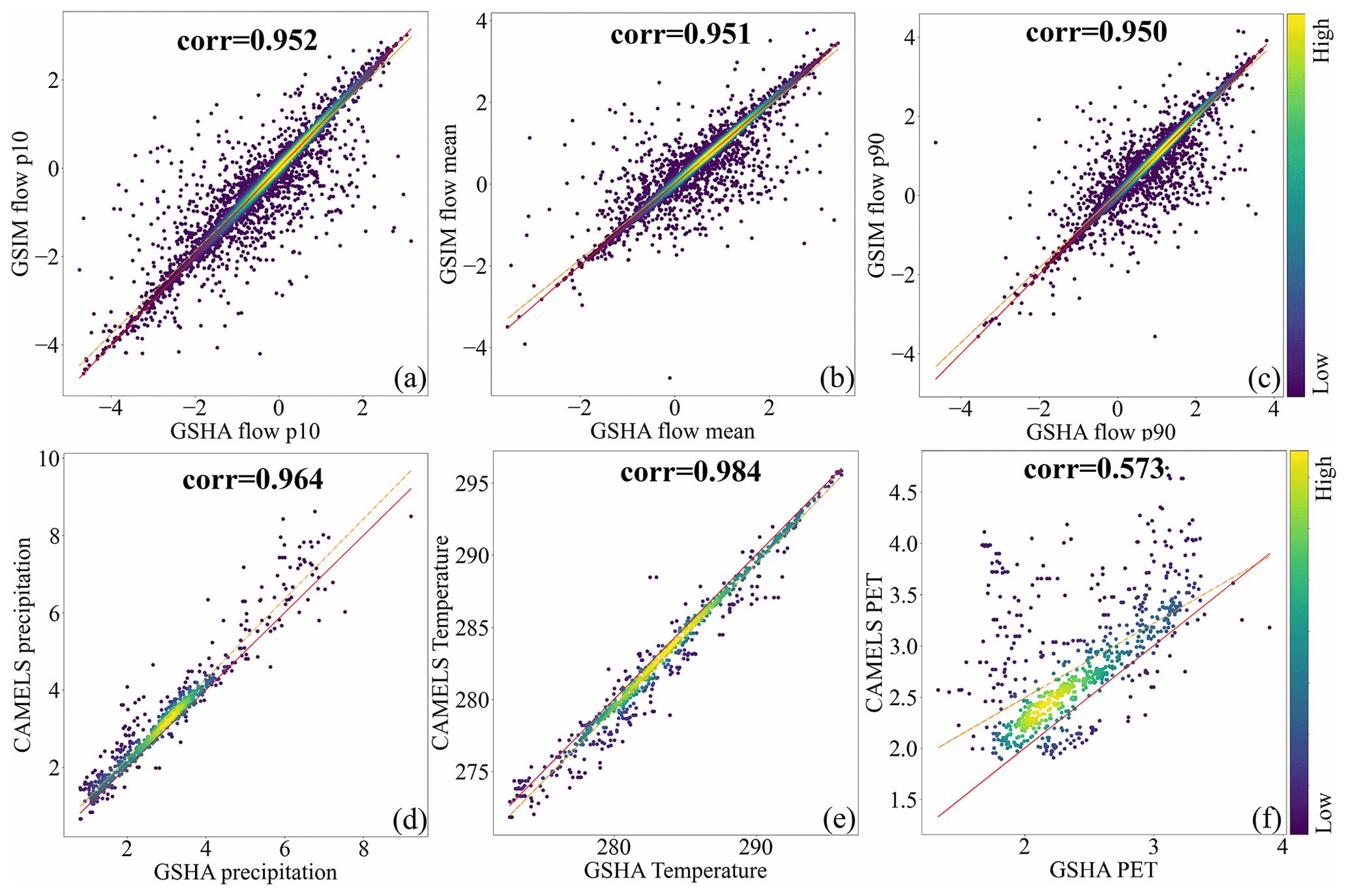
Figure 5 Validation of GSHA with GSIM streamflow characteristics (a, b, c) and CAMELS meteorological variables (d, e, f). “corr” in the panel is the Pearson correlation coefficient. The red line is the 1:1 line, while the dotted orange line is the fitting line of the scatter points. The color bar represents density of the sample points. The units on the x and y axes in (a), (b), and (c) are log10 m³ s⁻¹.

4.2 Uncertainty patterns for the GSHA meteorological variables

Figure 6 shows the distributions of the uncertainties for different variables, and the color bars are unified to allow for comparisons between different variables.

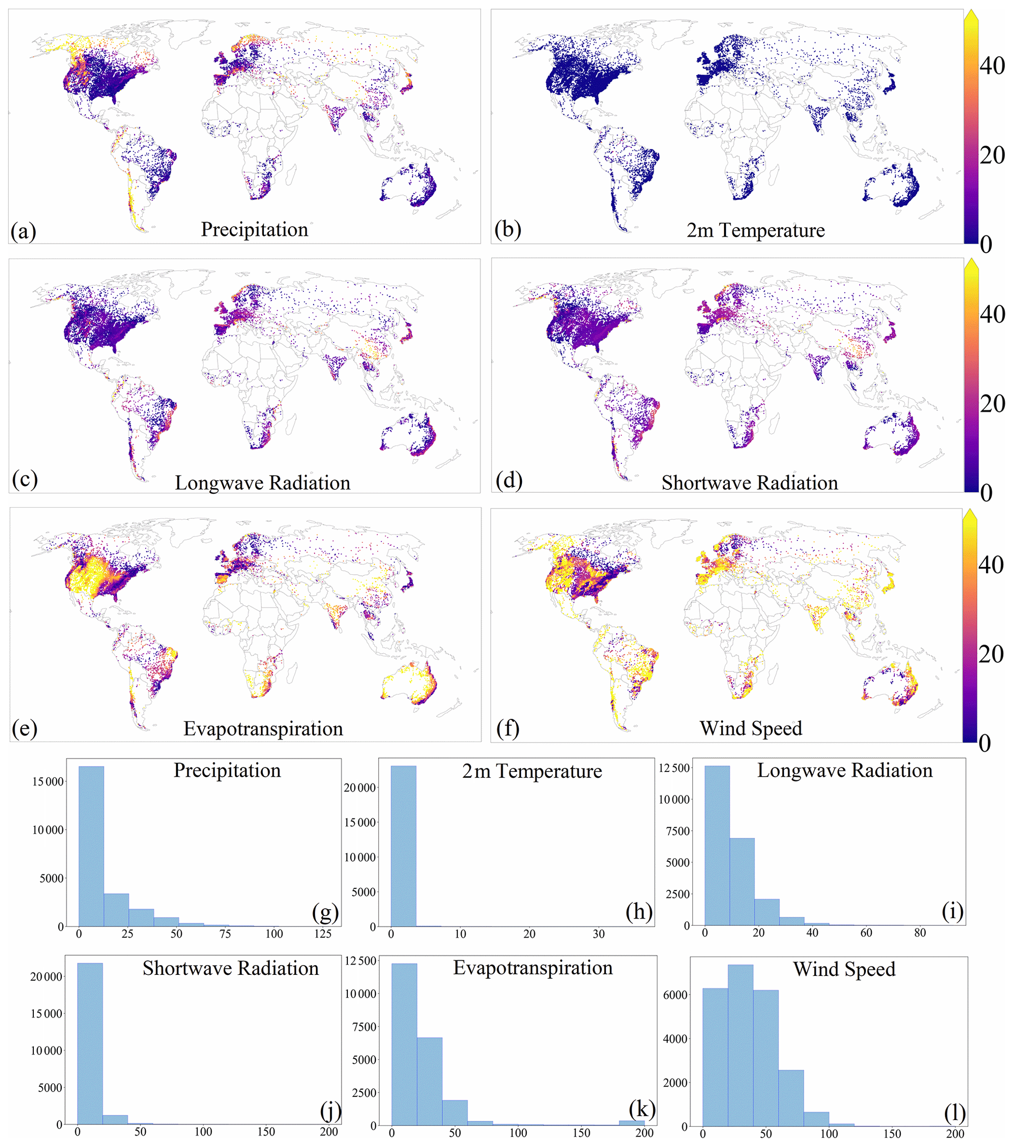
Figure 6 Global patterns of the uncertainty for the GSHA meteorological variables (in percentage). This includes the uncertainty for (a) precipitation (mm d⁻¹), (b) 2 m temperature (K), (c) longwave radiation (W m⁻²), (d) shortwave radiation (W m⁻²), (e) evapotranspiration (mm d⁻¹), and (f) wind speed (m s⁻¹) as well as uncertainty histograms for (g) precipitation, (h) 2 m temperature, (i) longwave radiation, (j) shortwave radiation, (k) evapotranspiration, and (l) wind speed.

Generally, among all variables, air temperature (Fig. 6b and h) shows the minimum uncertainty (<5 %), suggesting high consistency of air temperature estimates from different datasets. The uncertainty for wind speed (Fig. 6f) is the highest among all variables. Uncertainties for other variables show strong spatial variability. For example, uncertainties for precipitation are high in high-latitude or mountainous areas like the Rocky Mountains, northern Europe, the Alps, and the Andes (Fig. 6a). This is reasonable because limited access to in situ observations and the misestimation of snow (Schreiner-McGraw and Ajami, 2020) can contribute to precipitation estimation errors, while the data sources show relatively high consistency (uncertainty≤25 %) in other parts of the world (Fig. 6g). For radiation, as solar/shortwave radiation is largely affected by sky conditions, uncertainties are high in regions with fewer clear skies, including southwest China and its surrounding areas, high-latitude regions of the Northern Hemisphere, and Europe (Brun et al., 2022). These places are also subject to high thermal/longwave radiation uncertainties for similar reasons (Fig. 6c). Land cover, including vegetation and artificial surfaces, is another factor influencing surface net radiation through the albedo effect (Hu et al., 2017); thus, for heavily vegetated and urbanized areas, such as the Amazon region and east coastal Australia, uncertainties for both longwave and shortwave fluxes are also relatively high. Nevertheless, Fig. 6i and j demonstrate that for the majority of watersheds, radiation uncertainties are <25 %, indicating that the radiation data sources are generally consistent with each other. ET uncertainties are generally larger than the above variables (Fig. 6e and k) and are particularly prominent in dry areas of the globe, e.g., central North America, northern Andes, central Asia, and Australia's grasslands and deserts. It is also prominent in agriculture intensive regions like India and the northern part of China (Sörensson and Ruscica, 2018), where agricultural irrigation may be the contributing factor to the ET uncertainty. The spatial distributions of wind speed do not seem to show clear regional patterns (Fig. 6f), and uncertainty values of wind speed are generally larger over the majority of watersheds (Fig. 6l). Nevertheless, the uncertainties are low in Appalachia and northern Europe and are high in most parts of Brazil, the Andes, Africa, eastern and southern parts of Asia, and Australia (Fig. 6f). As we already selected relatively high-quality datasets for the variables, these areas might be calling for more attention by the LSH developers, while providing possible explanations for the inconsistencies in interpreting results or understanding the challenges in estimating model parameters by the LSH users.

Apart from the spatial patterns above, we also investigated the emergent patterns of the uncertainties. Existing studies indicate small basins can show larger uncertainties due to coarse resolution data inputs (Kauffeldt et al., 2013), while sub-grid variabilities might be offset by averaging over large watersheds. We plotted the uncertainty against watershed areas in Fig. 7, which verifies that for most variables, the uncertainty declines as the watershed area increases. Figure 7 also reveals some interesting patterns that have rarely been discussed in existing studies. For example, the most obvious decline in data uncertainty with area came from ET (green). ET is highly dependent on and significantly affected by land surface spatial heterogeneity; thus, it benefits the most from spatial averaging for large river basins. Longwave radiation uncertainty (red) experiences a moderate decline, likely due to its linkage with land surface complexity and cloud conditions. Shortwave radiation and precipitation uncertainty show a similar decline pattern (blue and purple), which is possibly related to their strong ties to cloud cover. Temperature has a low uncertainty, and its relationship to watershed area is also not obvious. Wind speed uncertainty only declines slightly as the area increases, and this may be because wind speed uncertainty can be traced back more to the atmospheric circulation patterns instead of land surface conditions, thus showing a non-prominent relationship with watershed area. Overall, GSHA provides uncertainty estimates that capture these prominent patterns, which can be helpful for hydrologic modelers and users.

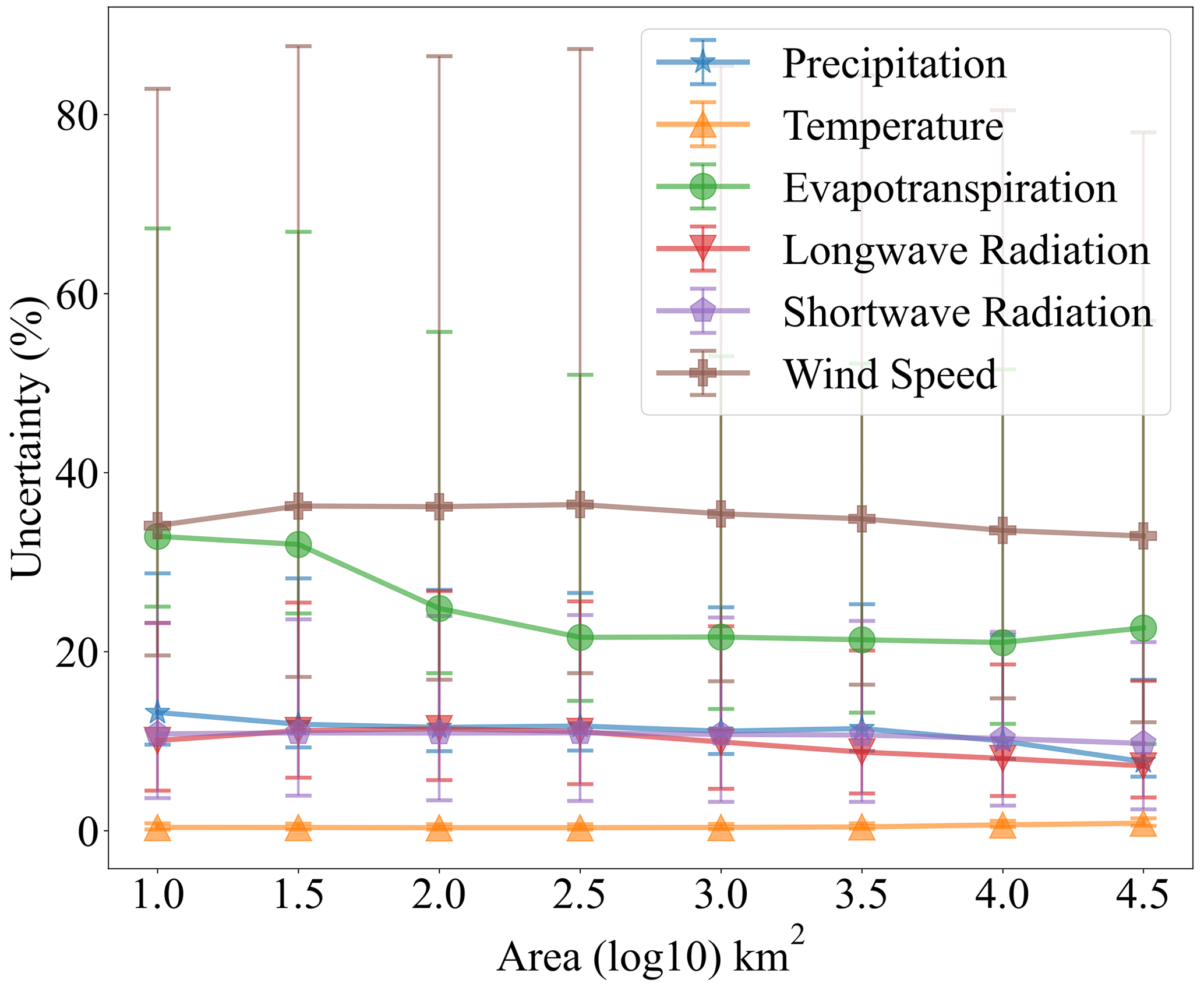
Figure 7 Relationship between variable uncertainties and watershed areas. The markers indicate mean values of the variable uncertainties in watersheds smaller than the corresponding x axis value. The error bars represent the range between 25th and 75th percentiles of the uncertainty values.

4.3 Natural and human-managed watersheds and changing patterns

We also demonstrate the other key features of GSHA by categorizing global watersheds into natural and human managed and by more prominently showing their temporal shifts in Fig. 8. Overall, the majority of human-managed watersheds are located in the US, Europe, and other regions with intensive industrial or agricultural activities such as East and South Asia (Fig. 8a and b). During 2001–2015, 46.89 % of the watersheds remained natural, while another 47.62 % under human management in 2001 remained in the category throughout the study period (Fig. 8d). Generally, the Northern Hemisphere has a larger proportion of human-managed watersheds, while watersheds in the less populated and urbanized Southern Hemisphere largely remain natural.

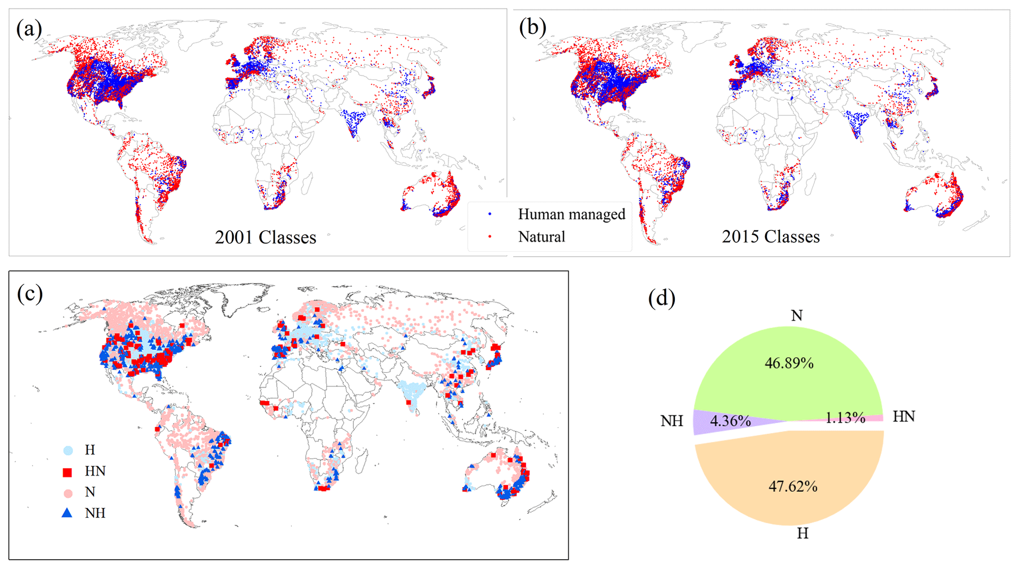
Figure 8 Classification of natural and human-managed watersheds in 2001 (a) and 2015 (b). Changes in watershed categories are illustrated by (c) and (d). H and N in (c) and (d) represent watersheds that remained human managed or natural from 2001 to 2015; NH and HN represent those changing from natural to human managed and from human managed to natural, respectively.

Noticeably, 4.36 % of GSHA watersheds switched from natural to human managed (1011 watersheds), and the remaining 1.13 % changed back to natural states from human managed during 2001–2015. For instance, watersheds in the middle and lower Yangtze River area and northeastern China show a shift from human managed to natural state where ecological restoration projects were in place (Qu et al., 2018; Zhang et al., 2015). Although the time span of GSHA LULC dynamics restricted the change detection for developed countries as their urbanization and infrastructure development have long been completed, and for fast emerging economies after 2015, the time series were also missing; nevertheless, the changing human activities captured by GSHA may be helpful in understanding streamflow changes, including flood characteristics (Yang et al., 2021; Zhang et al., 2022).

We further used several examples to illustrate the changing status of GSHA watersheds (Fig. 9). Figure 9a and b show a watershed located in northeast China, where the rapid increase in cropland shifted the watershed from natural states to human managed in recent years. Figure 9c and d correspond to a mountainous area in Sichuan Province, China, which became human managed due to the construction of a reservoir in 2006. For another case in northeast China (Fig. 9e and f) and a USGS case (Fig. 9g and h), the watersheds shifted from human managed to natural, which is mainly manifested by the reduction in cropland fraction due to environmental policy. For instance, afforestation in response to the application of a sustainable agriculture policy (Du et al., 2023) during 2000–2010 in Changbai Mountains, where the watershed in Fig. 9e and f is located, significantly increased the forest cover and might bring a decline in human disturbance in the form of land use (Zhang and Liang, 2014). These results highlight the shifting watershed status that requires further attention from LSH users, which is encapsulated in GSHA v1.0 and will be continuously improved in the future.

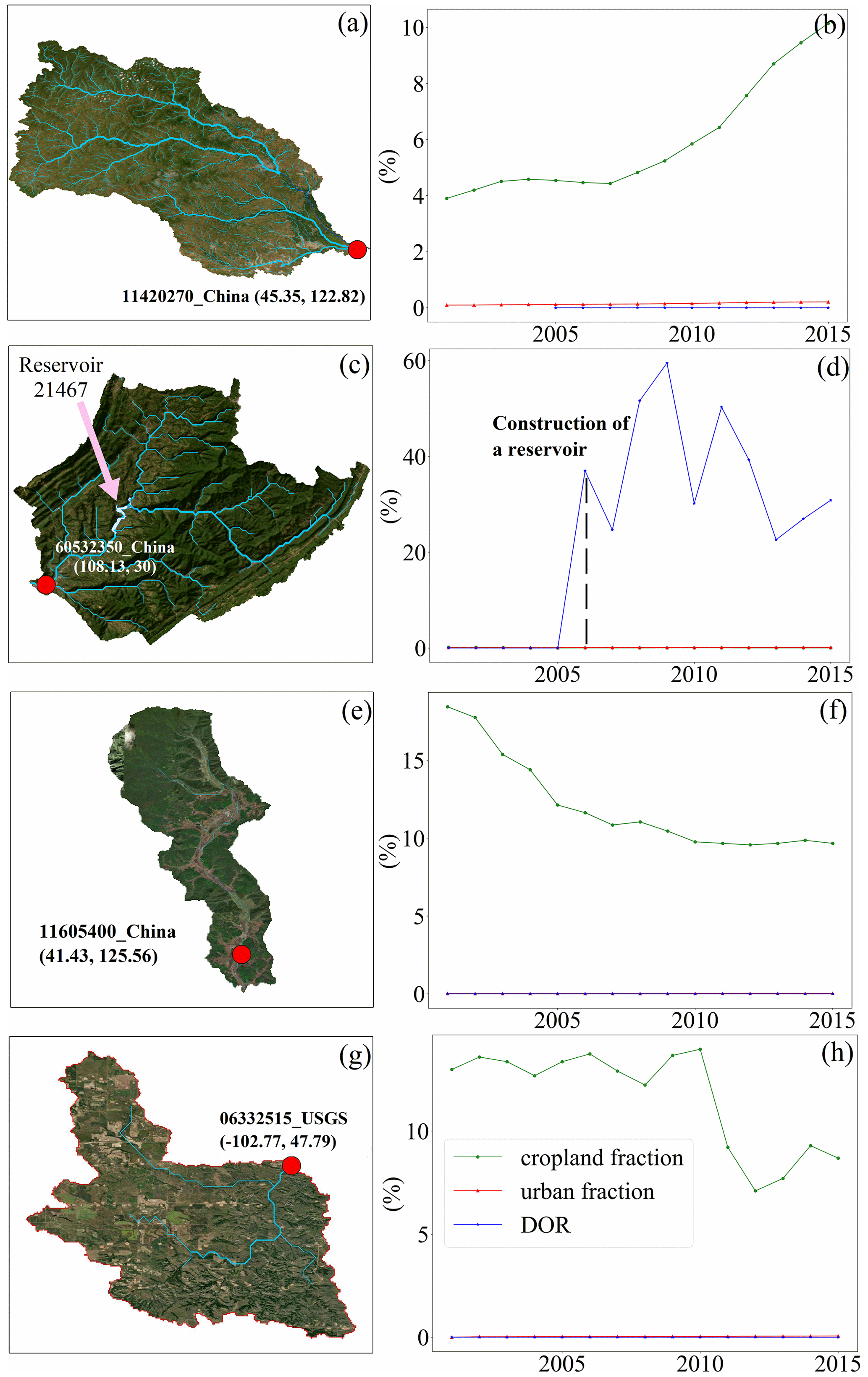
Figure 9 Cases for shifting status of the watershed classification. Panels (a) and (b) correspond to 11420270_China and (c) and (d) correspond to 60532350_China, both of which changed from the natural to human-managed category. Panels (e) and (f) represent11605400_China and (g) and (h) correspond to 06332515_USGS watershed changing from human-managed to natural watershed.

4.4 Changing runoff coefficient patterns derived from GSHA

Finally, we also analyzed the global pattern in the trend of runoff coefficient (RC) as a brief demonstration of what GSHA can offer, out of many potential uses. RC is defined as $R/P$, where R denotes runoff (mm) and P denotes precipitation (mm). Figure 10a shows that regions with high RC (i.e., a large proportion of rainfall goes into rivers instead of being evaporated or consumed) are in east Asia and North America, most parts of Europe, the west coast of North America, and the Amazon, in general agreement with the aridity patterns across the globe. For arid/semiarid areas and places with intense water use (e.g., western US, eastern Brazil, Australia, Africa), RC is low, meaning most of the precipitation does not reach the gauged river.

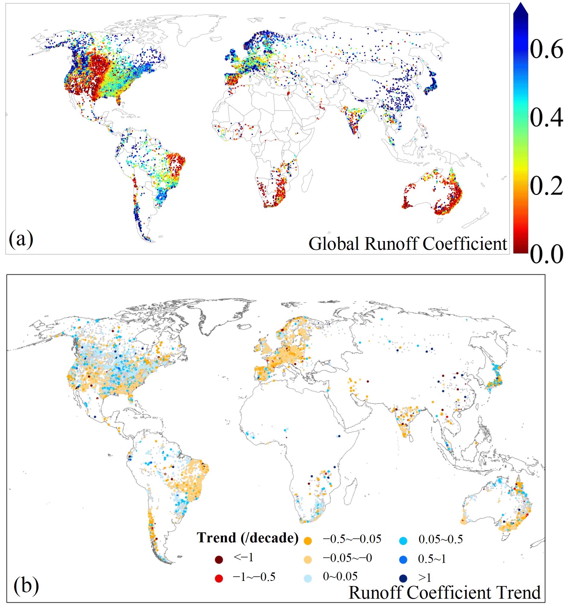
Figure 10 Patterns of runoff coefficient (a) and its trend (b). Only watersheds with a statistically significant trend (p<0.05) are shown with colors in (b); the small and large points represent 95 % (p<0.05) and 90 % significance levels (p<0.1), respectively. Note that the temporal coverage is different for different gauges; we refer readers to the GSHA temporal coverage for interpretation of the patterns. The figure illustrates 18 987 GSHA watersheds. Watersheds with less than 10 years of indices calculated from over 250 valid observations per year, as well as with runoff coefficient trend over 20 decade⁻¹, are not shown in panel (b).

We found that RC generally remained stable over the past decades (i.e., gray dots in Fig. 10b; >80 % of the gauges did not observe a statistically significant trend), while 4252 watersheds observed a statistically significant trend in RC at 95 % level (5690 watersheds at 90 % level). Among them, decreasing RC is more widespread than increasing RC. The most pronounced decreasing trends are observed in Europe, India, eastern Brazil, Chile, eastern Australia, and the Euphrates and Tigris rivers, which largely correspond to regions with known intense agricultural, industrial, and residential water use that may have reduced the river water. We note that the global RC trend patterns were different from a recent study that showed mostly increasing RC in the high latitudes, central North America, eastern Australia, and Europe (Xiong et al., 2022). Given Xiong et al. (2022) used estimated runoff while we used runoff directly from gauge observations, it is likely that the concerning water availability issues in the context of increasing human water use may not be fully captured by existing studies. Regional studies also tend to show inconsistent results. For example, a study based on models incorporating climate change and land use change but ignoring human water consumptions suggested that deforestation and urbanization generally increase RC (Lucas-Borja et al., 2020), while another study identified a significant decreasing trend for RC by focusing on cases with intense irrigational water use (Banasik and Hejduk, 2012). These collectively preclude a clear identification of consistent RC trends (Velpuri and Senay, 2013) and a clear causal factor attribution analysis given the complexity of the anthropogenic factors. As such, GSHA may offer a new path to fill in the gap of disentangling the influences of large-scale water use on decreasing RC.

5 Code and data availability

GSHA v1.0 is openly available at https://doi.org/10.5281/zenodo.8090704 and https://doi.org/10.5281/zenodo.10433905 (Yin et al., 2023a, b). The codes involved in the workflow for generating GSHA will be available upon reasonable request to the corresponding author. The publicly available gauge databases used in this scrapping process include R-ArcticNET (http://www.r-arcticnet.sr.unh.edu/v4.0/AllData/index.html, Water Systems Analysis Group, 2022), Australian Bureau of Meteorology (http://www.bom.gov.au/waterdata/, Australian Bureau of Meteorology, 2022), Brazil National Water Agency (https://www.snirh.gov.br/hidroweb/serieshistoricas, Brazil National Water Agency, 2022), Canada National Water Data Archive (https://www.canada.ca/en/environment-climate-change/services/water-overview/quantity/monitoring/survey/data-products-services/national-archive-hydat.html, Canada National Water Data Archive, 2022), Chile Center for Climate and Resilience Research (https://explorador.cr2.cl/, Chile Center for Climate and Resilience Research, 2022), The Global Runoff Data Centre (https://portal.grdc.bafg.de/applications/public.html?publicuser=PublicUser, The Global Runoff Data Centre, 2022), India Water Resources Information System (https://indiawris.gov.in/wris/#/RiverMonitoring, India Water Resources Information System, 2022), Japanese Water Information System (http://www.river.go.jp/, Ministry of Land, Infrastructure, Transport and Tourism, 2022), Spain Annuario de Aforos (http://datos.gob.es/es/catalogo/e00125801-anuario-de-aforos/resource/4836b826-e7fd-4a41-950c-89b4eaea0279, Anuario de Aforos Digital – datos.gob.esm, 2022), Thailand Royal Irrigation Department (http://hydro.iis.u-tokyo.ac.jp/GAME-T/GAIN-T/routine/rid-river/disc_d.html, Thailand Royal Irrigation Department, 2022), and the U.S. Geological Survey (https://labs.waterdata.usgs.gov/visualizations/gages-through-the-ages, U.S. Geological Survey, 2022). The Chinese Hydrology Project data were provided by the authors of the dataset (Henck et al., 2010; Schmidt et al., 2011).

6 Conclusions

Large sample hydrology (LSH) datasets play a critical role in data-driven analyses and model parameter estimation for hydrological studies. From MOPEX (Duan et al., 2006) to Caravan (Kratzert et al., 2023), significant efforts have been made to improve the comprehensiveness of LSH, yet issues related to data spatial coverage, uncertainty estimates, and human activity dynamics remain to be solved. This study complements existing LSH with a new synthesis dataset named the Global Streamflow characteristics, Hydrometeorology, and catchment Attributes for large sample river-centric studies (GSHA v1.1).

To summarize, GSHA contributes the following aspects to the LSH development.

1. It includes streamflow indices, hydrometeorological data, and surface characteristics data for 21 568 gauges compiled from 13 agencies worldwide, which represents one of the most comprehensive LSH by far.

2. We incorporated multiple data sources to provide uncertainty estimates for each meteorological variable (including precipitation, 2 m air temperature, radiation, wind, and ET). The spatial patterns and the relationship between the uncertainty and the watershed characteristics GSHA reveals may be helpful in identifying inconsistencies among data-driven studies or biases for model parameter estimation studies using existing LSH.

3. Dynamic data are provided for previously static data descriptors for land cover changes including urban, cropland, and forest fractions, as well as reservoir storage change including storage capacity and degree of regulation.

Although GSHA does not cover watersheds of <25 km² or the dynamics of cryosphere variables (e.g., glacier and permafrost) that have become increasingly important in terrestrial hydrological changes and although the time spans for the dynamic descriptors of LULC are unable to cover the critical periods for the advanced and less-advanced economies due to the constraints with existing LULC data, GSHA is expected to be utilized to provide the following insights.

1. The uncertainty patterns vary between variables and geographical regions, indicating that the interpretation of model and analysis results need to consider inconsistencies of raw data apart from looking into the methodologies and patterns themselves.

2. Although most watersheds have remained natural or human managed throughout the GSHA time span, a considerable number of watersheds shifted between the two categories, which can be ascribed to urbanization, cropland increase, reservoir construction, and ecological restoration, such as returning farmland to natural states, and these can be clearly manifested using GSHA.

3. Analysis with runoff coefficient reveals that among gauges with a statistically significant trend, a greater portion experienced a declining RC trend than an increase trend. This pattern revealed by GSHA can be used to further study water availability issues in a changing climate.

As our knowledge on the above processes continues to improve, we expect that future versions of GSHA will be continuously updated. Finally, better hydrological data sharing is crucial to advance global change hydrology studies.

Appendix A: Spatial patterns of GSHA meteorological variables

Figures A1 and A2 show the spatial distributions of GSHA meteorological variables and selected streamflow indices. The spatial pattern derived from each individual data source is plotted separately.

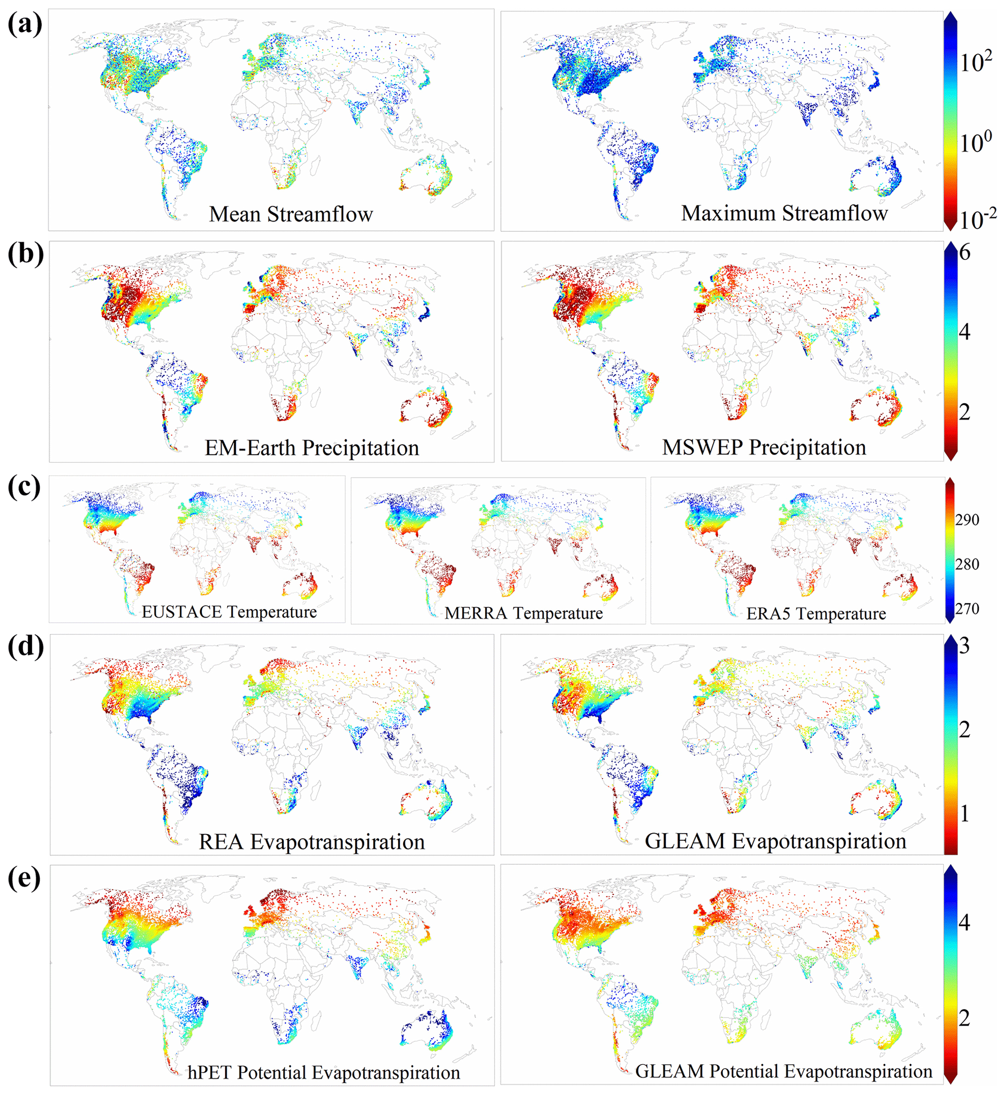
Figure A1 Spatial distribution of streamflow indices (a, m³ s⁻¹), precipitation (b, mm d⁻¹), 2 m air temperature (c, K), actual ET (e, mm d⁻¹), and potential ET (f, mm d⁻¹).

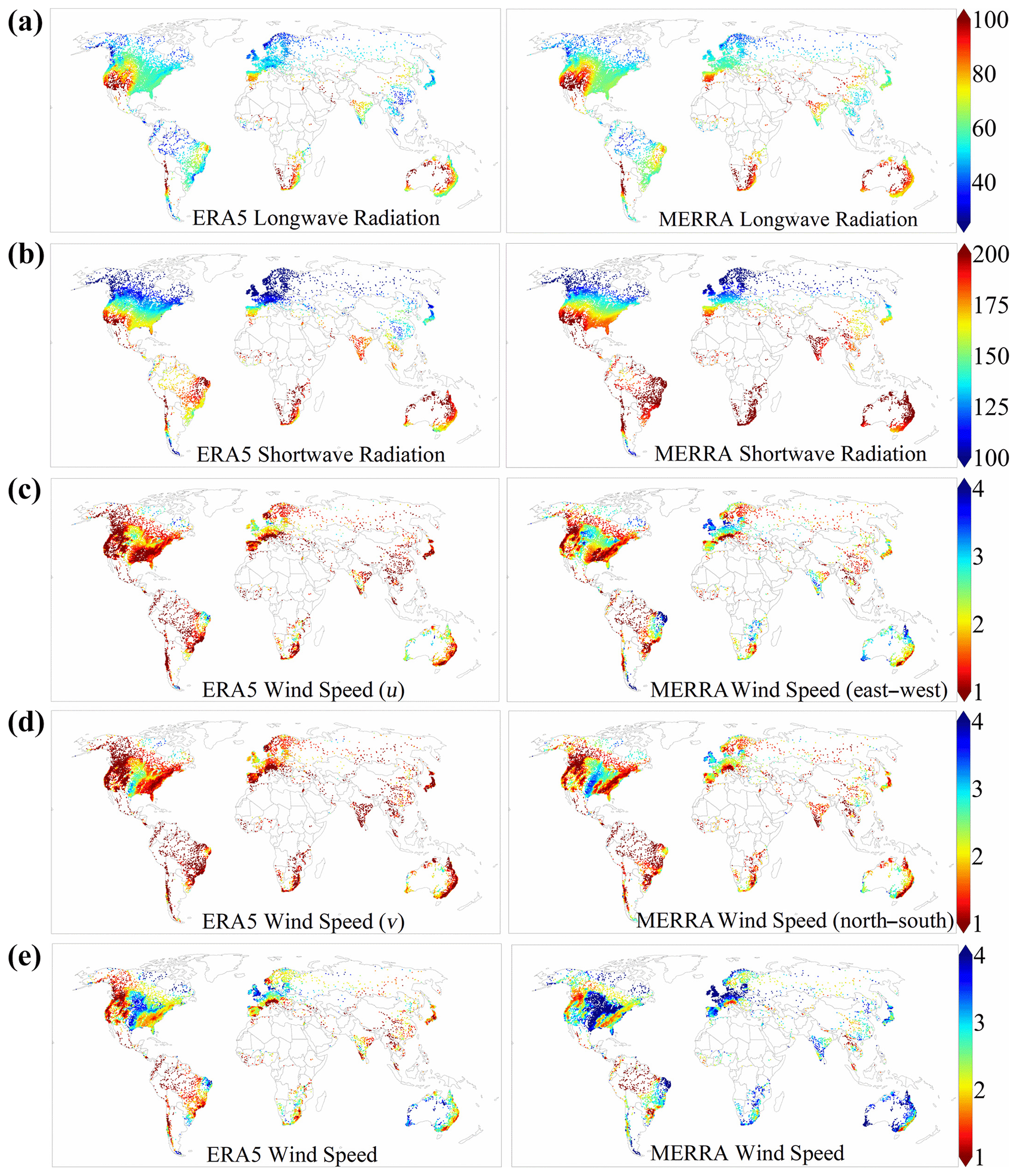
Figure A2 Spatial distribution of longwave radiation (a, W m⁻²), shortwave radiation (b, W m⁻²), wind u (c, m s⁻¹) and v components (d, m s⁻¹), and wind speed (e, m s⁻¹).

Appendix B: Validation results of watershed areas

The validation results with BOM, HYDAT, GRDC, and USGS on watershed areas are plotted in Fig. B1, where the mismatches between GSHA areas and the officially reported areas are shown. Before removing the mismatched watersheds, their correlation coefficients are 0.960, 0.840, 0.709, and 0.905, respectively, as shown in Fig. B1a–d. After removing the mismatched watersheds, correlation coefficients for all three agencies reach 0.999, as shown in Fig. B1e–h. As we traced the MERIT-Basins (Lin et al., 2019) for our watershed delineation, the mismatches are believed to occur when the gauge is located in the vicinity of the intersection point of a river reach and its main stream, which makes it difficult to determine which reach the gauge belongs to while matching the gauge to the MERIT river network. This explains why in Fig. B1 most of the mismatches appear in relatively small areas. As we do not have access to all official watershed areas, and Fig. B1a–d suggest that matching qualities differ among the agencies, to simply remove the mismatched watersheds or to modify them might put the samples in the dataset under an inconsistent standard. Additionally, some agencies such as GRDC experienced some updates of their gauge locations and upstream areas; thus, watershed boundaries in all datasets mentioned might come with uncertainties. Therefore, we gave the watersheds as “unverified”, “verified match”, and “verified mismatch” identifiers to allow users to flexibly filter the watersheds.

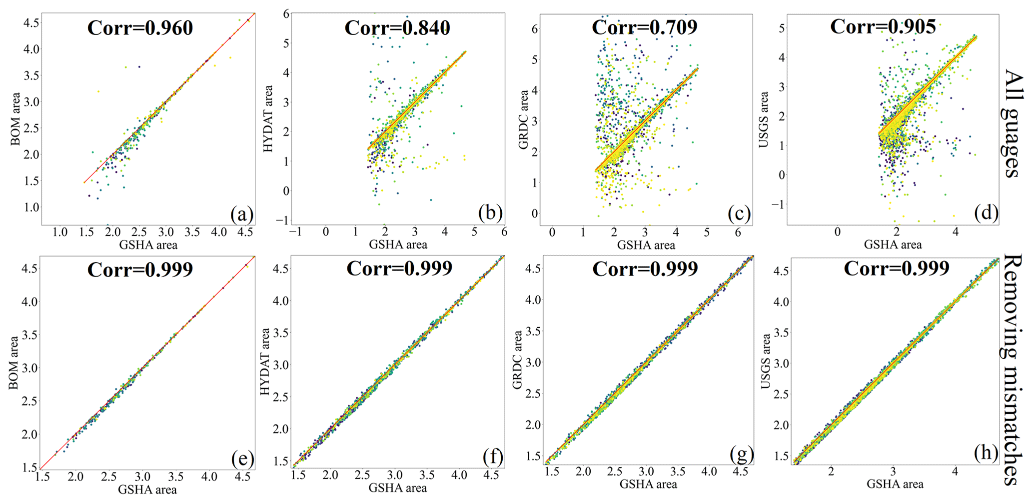
Figure B1 Validation of GSHA with officially reported areas of BOM (a, e), HYDAT (b, f), GRDC (c, g), and USGS (d, h). Panels (a–d) are the results before removing the mismatched watersheds, and panels (e–h) present results after removing the mismatched watersheds. The Pearson correlation coefficient are represented by “Corr” in the figure. The areas are represented by the unit of (log 10 km²).

Appendix C: Potential evapotranspiration uncertainty

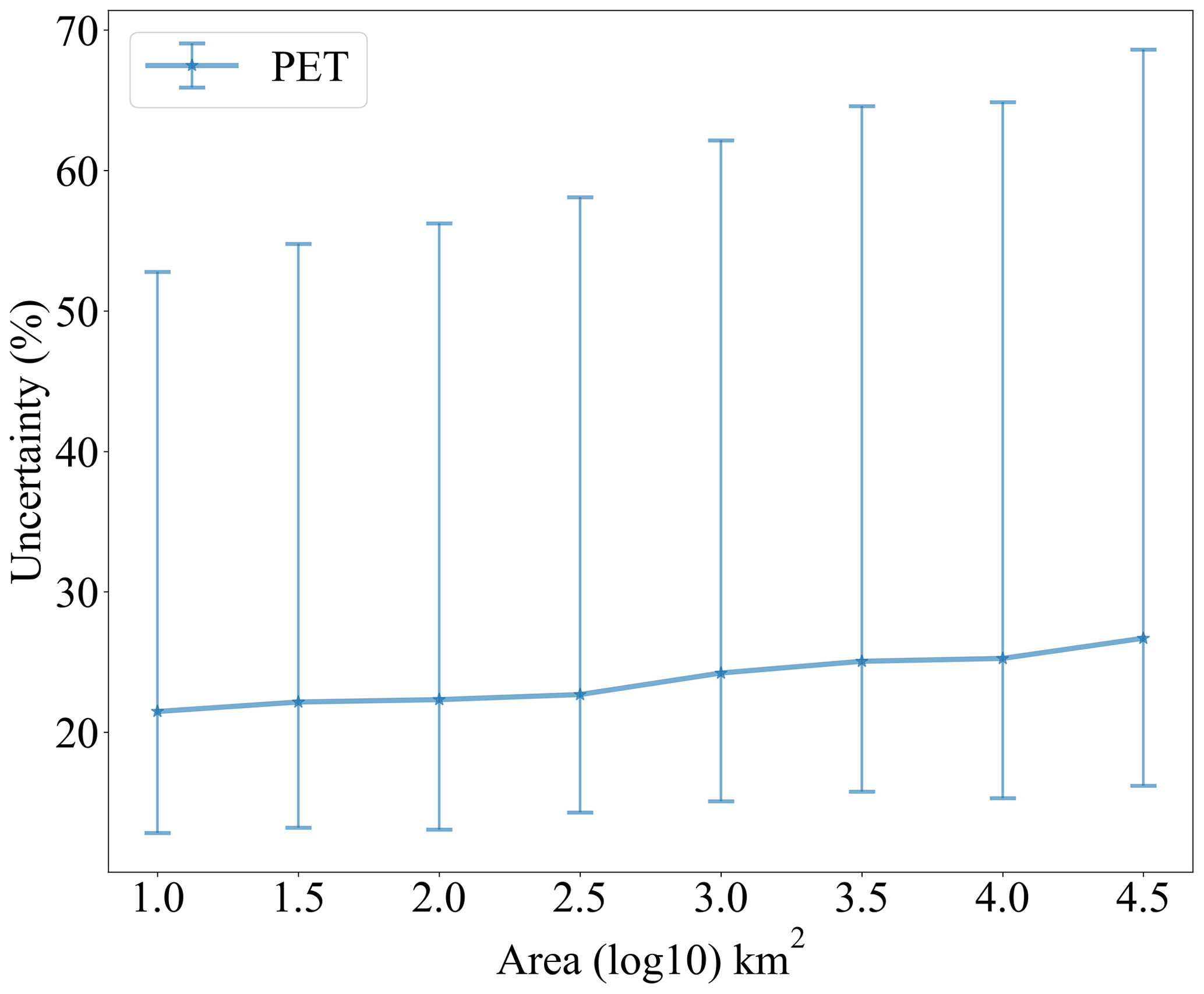
The spatial and numerical distributions of potential evapotranspiration (PET) uncertainties are illustrated in Figs. C1 and C2. PET uncertainty is high compared with other variables (see Sect. 4.3). The majority of high PET uncertainty watersheds are in dry areas, but since it is calculated from meteorological variables, exceptions exist for places including eastern Pacific coast, where the climate is dry but PET uncertainty is low, and India, which is located in a wet climate zone but has high PET uncertainty. As demonstrated by Fig. C3, PET uncertainty does not decrease with the increase in watershed area, probably because PET is calculated from various variables and the calculation over large watersheds involves more uncertainties for individual grids.

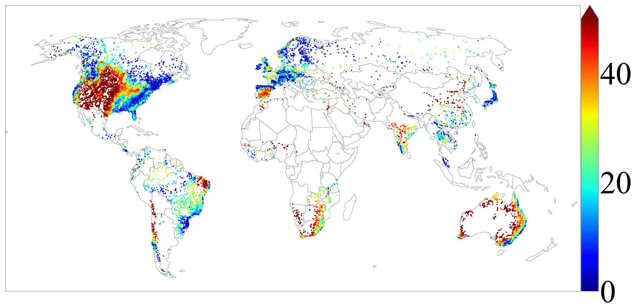
Figure C1 Spatial pattern of potential evapotranspiration (PET) uncertainty.

Figure C2 Numerical distribution of PET uncertainty.

Figure C3 Relationship of PET uncertainty to watershed area.