Metazoan zooplankton in the Bay of Biscay: a 16-year record of individual sizes and abundances obtained using the ZooScan and ZooCAM imaging systems

This paper presents two metazoan zooplankton datasets obtained by imaging samples collected on the Bay of Biscay continental shelf in spring during the PELGAS (PELagique GAScogne) integrated surveys over the 2004–2019 period. The samples were collected at night with a 200 µm mesh-size WP2 net fitted with a Hydrobios (back-run stop) mechanical flowmeter and hauled vertically from the sea floor to the surface, with the maximum depth set at 100 m when the bathymetry was deeper than this. The first dataset originates from samples collected from 2004 to 2016 and imaged on land with the ZooScan and is composed of 1 153 507 imaged and measured objects. The second dataset originates from samples collected from 2016 to 2019 and imaged onboard the R/V Thalassa with the ZooCAM and is composed of 702 111 imaged and measured objects. The imaged objects are composed of zooplankton individuals, zooplankton pieces, non-living particles and imaging artefacts ranging from 300 µm to 3.39 mm in equivalent spherical diameter which were individually imaged, measured and identified. Each imaged object is geolocated and associated with a station, a survey, a year and other metadata. Each object is described by a set of morphological and grey-level-based features (8 bit encoding, 0 = black, 255 = white), including size, that were automatically extracted from each individual image. Each object was taxonomically identified using the web-based application Ecotaxa with built-in random-forest and CNN-based semi-automatic sorting tools, which was followed by expert validation or correction. The objects were sorted into 172 taxonomic and morphological groups. Each dataset features a table combining metadata and data at individual-object granularity from which one can easily derive quantitative population and community descriptors such as abundances, mean sizes, biovolumes, biomasses and size structure. Each object's individual image is provided along with the data. These two datasets can be used in combination for ecological studies, as the two instruments are interoperable, or they can be used as training sets for ZooScan and ZooCAM users. The data presented here are available at the SEANOE dataportal: https://doi.org/10.17882/94052 (ZooScan dataset, Grandremy et al., 2023c) and https://doi.org/10.17882/94040 (ZooCAM dataset, Grandremy et al., 2023d).

1 Introduction

Metazoan planktonic organisms, hereafter referred to as zooplankton, encompass an immense diversity of life forms which have successfully colonized the entire ocean, from eutrophic estuarine shallow areas to the oligotrophic open ocean and from the sunlit ocean to hadal depths. Their body sizes span 5 to 6 orders of magnitude in length: from µm to tens of metres (Sieburth and Smetacek, 1978). Zooplankton plays a pivotal role in marine ecosystems (Banse, 1995). It transfers the organic matter produced in the epipelagic domain by photosynthesis to the deeper layers of the ocean (Siegel et al., 2016) by producing fast-sinking aggregates (Turner, 2015) and by diel vertical migration (Steinberg et al., 2000; Ohman and Romagnan, 2016). Zooplankton therefore participates in mitigating the anthropogenic carbon dioxide buildup in the atmosphere that is responsible for climate change. Moreover, zooplankton is an exclusive trophic resource for commercially important fish during their larval stage, so a shift in zooplankton species or phenology can have dramatic effects on recruitment (e.g. for North Sea cod; Beaugrand et al., 2003). In addition, it is a major trophic resource for adult small planktivorous pelagic fish known as forage fish (van der Lingen, 2006). Recent studies suggest that zooplankton dynamics may have a significant effect on small pelagic fish population dynamics and individual body condition (Brosset et al., 2016; Menu et al., 2023) and therefore impact wasp-waist ecosystem-based fisheries and socio-ecosystems that are dependent on those fisheries worldwide (Cury et al., 2000).

Despite zooplankton being of such global importance in both climate change effects on ecosystems and the management of fisheries (Chiba et al., 2018; Lombard et al., 2019), it is still technically difficult to monitor compared to other marine ecological compartments. Zooplankton biomass, diversity and spatio-temporal distributions cannot be estimated from spaceborne sensors, unlike those of phytoplankton (Uitz et al., 2010), commercial exploitation data of zooplankton do not exist yet, unlike the corresponding data for fish. One noticeable exception is the CPR Survey network, which enables zooplankton data generation at spatio-temporal scales that are fine enough to study climate change and diversity-related zooplanktonic processes (Batten et al., 2019). Yet, generating zooplankton data often requires dedicated surveys at sea, specific sampling instruments and trained taxonomic analysts. Moreover, besides actual observation, modelling zooplankton remains a challenging task due to the diversity of traits, such as life forms, life cycles, body sizes, and physiological processes, exhibited by zooplankton (Mitra and Davis, 2010; Mitra et al., 2014). However, over the past 2 decades, the development of imaging and associated machine-learning semi-automatic identification tools (Irisson et al., 2022) has greatly improved the capability of scientists to analyse long (Feuilloley et al., 2022), high-frequency (Romagnan et al., 2016) or spatially resolved (Grandremy et al., 2023a) zooplankton time series as well as trait-based data (Orenstein et al., 2022). Imaging and machine learning have particularly enabled the increased development of combined size and taxonomy zooplankton ecological studies (e.g. Vandromme et al., 2014; Romagnan et al., 2016; Benedetti et al., 2019). Yet, the use of these machine-learning tools is not trivial because they require abundant, scientifically qualified, sensor-specific training image data (i.e. a learning set and test set; Irisson et al., 2022) and complex hardware and software setups (Panaïotis et al., 2022). One good example of such an image dataset is the ZooScanNet dataset (Elineau et al., 2018), which features an extensive ZooScan (Gorsky et al., 2010) imaging dataset usable as a training set for ecologists as well as for imaging and machine-learning scientists.

The objective of this paper is to present two freely available zooplankton imaging datasets originating from two different instruments, the ZooScan (Gorsky et al., 2010) and the ZooCAM (Colas et al., 2018). These datasets originate from the PELGAS (PELagique GAScogne) integrated survey in the Bay of Biscay (Doray et al., 2018a), a continental shelf ecosystem supporting major European fisheries (ICES, 2021). Combined, these datasets make up a 16-year time series of sized and taxonomically resolved zooplankton, along with context metadata allowing the calculation of quantitative data, covering the whole Bay of Biscay continental shelf from the French coast to the continental slope and from the Basque Country to southern Brittany in spring. These datasets can be used for ecological studies (Grandremy et al., 2023a), machine-learning studies and modelling studies.

2 Methods

2.1 Sampling

Zooplankton samples were collected during successive PELGAS integrated surveys carried out over the Bay of Biscay (BoB) French continental shelf every year in spring from 2004 to 2019 onboard the R/V Thalassa. The aim of this survey is to assess small pelagic fish biomass and monitor the pelagic ecosystem to inform ecosystem-based fisheries management. Fish data, hydrology, phyto- and zooplankton samples, and megafauna sightings (marine mammals and seabirds) are concomitantly collected to build long-term spatially resolved time series of the BoB pelagic ecosystem. The PELGAS sampling protocols combine daytime en-route data collection (small pelagic fish and megafauna) with night-time depth-integrated hydrology and plankton sampling at fixed points. Detailed PELGAS survey protocols can be found in Doray et al. (2018a, 2021). The PELGAS survey datasets providing hydrological, primary producers, fish and megafauna data are available as gridded data in the SEANOE data portal (Doray et al., 2018b) at the following link: https://doi.org/10.17882/53389.

The number of zooplankton samples obtained per year varied between 41 (2005) and 65 (2019) due to adjustments in the sampling strategy and the weather conditions, with 889 zooplankton samples collected in total. From 2004 to 2006, samples were collected in the southern Bay of Biscay up to the Loire estuary only (Fig. 1). Sampling was carried out in vertical tows performed during the night using a 200 µ m mesh-size WP2 net, generally from 100 m depth (or 5 m above the seabed) to the surface. In 2004 and 2005, the targeted maximum sampling depth was 200 m. In 2004, 15 samples were collected deeper than 100 m, among which 11 were deeper than 120 m; in 2005, 20 samples were collected deeper than 100 m, among which 13 were deeper than 120 m. Before 2014, the sampled water volume was estimated by multiplying the cable length by the net opening surface (0.25 m²), whereas the net has been equipped with a Hydrobios back-run stop flowmeter since 2014. The samples originating from the 2004 to 2016 surveys were preserved in 4 % formaldehyde (final concentration) and analysed on land in the laboratory with the ZooScan, while they have been analysed live onboard with the ZooCAM since 2016.

2.2 Sample processing and analyses

2.2.1 Digitization with the ZooScan

Preserved samples were digitized with the ZooScan (Gorsky et al., 2010), a flatbed scanner generating 16 bit grey-level high-resolution images (2400 dpi, pixel size: 10.56 µm, image size: 15 × 24 cm equivalent to 14 200 × 22 700 pixels). It is well suited for the imaging of preserved organisms ranging in size from 300 µm to several centimetres. The ZooScan is run by the custom-made, ImageJ-based, ZooProcess software, which generates a single large image for each scan that contains up to 2000 organisms, depending on the size of the imaged organisms.

Prior to digitization, the seawater and formaldehyde solution was filtered through a 180 µm mesh sieve into a trash tank under a fume hood. The organisms were then gently but thoroughly rinsed with freshwater over the tank in the sieve. They were then size fractionated with a 1 mm sieve into organisms larger and smaller than 1 mm. This size-splitting step is recommended when using the ZooScan as it addresses the possible bias due to the underrepresentation of large objects caused by the necessary subsampling. Each size fraction was subsampled separately with a Motoda splitter to obtain two subsamples containing 500–1000 objects for the large-organism size fraction and 1000–2000 objects for the small-organism size fraction. To mitigate the number of overlapping objects, each subsample was imaged after the manual separation of objects on the scanning tray, as recommended in Vandromme et al. (2012). Overall, 699 samples were digitized following this protocol, corresponding to 1397 scans (one sample was not divided into size fractions as it did not contain organisms larger than 1 mm).

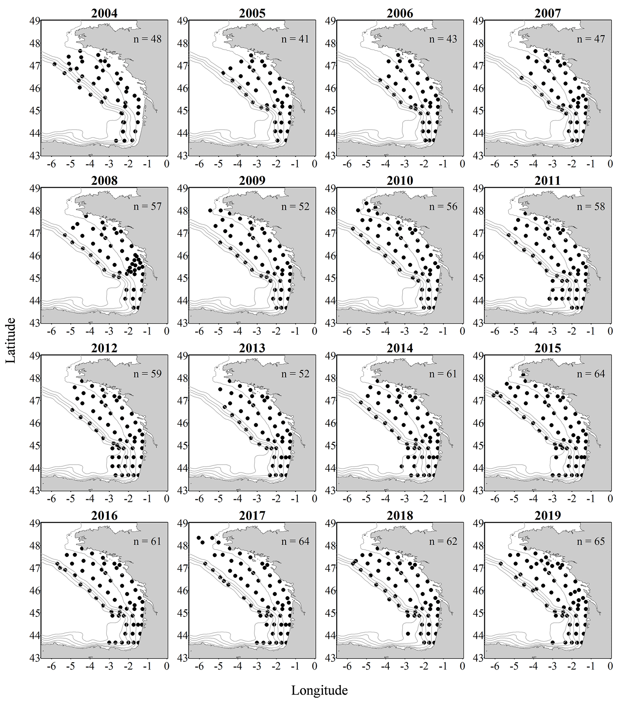
Figure 1 Metazoan zooplankton sampling locations during the PELGAS cruises in the Bay of Biscay from 2004 to 2019. The years with the poorest coverage are 2005 and 2006, with 41 and 43 sampling stations respectively, and the years with the best coverage are 2015, 2017 and 2019, with 64, 64 and 65 sampling stations respectively.

2.2.2 Digitization with the ZooCAM

The ZooCAM is an in-flow imaging instrument designed to digitize preserved as well as live zooplankton samples onboard, immediately after net collection (Colas et al., 2018). The ZooCAM features a cylindrical transparent tank in which the zooplankton sample is mixed with filtered seawater. Depending on the richness of the sample and the subsampling (if necessary), the volume of seawater can be adjusted between 2–7 L. The organisms were pumped at 1 L min⁻¹ from the tank to a flow cell inserted between a CCD camera (pixel size: 10.3 µm) and a red LED flashing device, where they were imaged at 16 fps. Given the flow cell volume, the size of the field of view, the imaging frequency and the flow rate, all the seawater volume containing the organisms was imaged (Colas et al., 2018). Before all the initial volume was imaged, the tank and the tubing were carefully and thoroughly rinsed with filtered seawater to ensure the imaging of all the organisms poured into the tank. For each sample, the ZooCAM generates a stack of small-size (∼ 1 MB) raw images that are subsequently analysed with the ZooCAM software. Depending on the initial water content of the tank and the rinsing, a ZooCAM run can generate up to 10 000 raw images from which the individual organism vignettes will be extracted. A ZooCAM run on a live sample often generates up to 5000–10 000 vignettes of individual organisms. It is very important to subsample the initial samples with a dichotomic splitter (a Motoda splitter was used here) to ensure that the object concentration in subsamples is low enough to reduce the risk of imaging overlapping objects and avoid any dependency on the water volume imaged when reconstructing quantitative estimates of zooplankton, as the initial and rinsing volumes are variable. Overall, 190 samples were digitized live onboard with the ZooCAM.

2.3 Image processing

Both instruments generate grey-level working images (8 bit encoding, 0 = black, 255 = white). In both cases, image processing consisted of (i) a “physical” background homogenization in which an empty background image was subtracted from each sample image (one for ZooScan and as many as there were raw images for ZooCAM), (ii) a thresholding of each raw image (the threshold value was 243 for ZooScan and 240 for ZooCAM), and (iii) the segmentation of each object imaged. The ZooProcess software was set to detect and segment objects with an area equal to or larger than 631 pixels, whereas the ZooCAM software was set to detect objects with an area equal to or larger than 667 pixels, which in both cases equals 300 µm equivalent spherical diameter (ESD), or a biovolume of 0.014 mm³ (using a spherical biovolume model; Vandromme et al., 2012).

Morphological features were then extracted for each detected object. Features generated by the ZooScan are defined in Gorsky et al. (2010) and those generated by the ZooCAM are defined in Colas et al. (2018). ZooScan images were processed with the ZooProcess v7.39 (4 October 2020) open-source software. ZooCAM images were processed with the proprietary ZooCAM custom-made software, which uses the MIL (Matrox Imaging Library, Dorval, Québec, Canada) as the individual-object processing kernel. Each detected object was finally cropped from the working sample images and saved as a unique labelled vignette in a sample-specific folder, along with a sample-specific single text file containing the object features arranged as a table with objects arranged in lines and features in columns.

2.4 Touching objects

ZooProcess features a tool that enables the digital separation of possibly touching objects in the final image dataset for each sample. As touching objects may impair abundance and size-structure estimations (Vandromme et al., 2012), remaining touching objects were searched for in the individual vignettes from the ZooScan and were digitally manually separated with the ZooProcess separation tool to improve the quality of further identifications, counts and the size structure of zooplankton. The ZooCAM software does not offer such a tool.

2.5 Taxonomic identification of individual images

All individual vignettes from both instruments were sorted into two instrument-specific separated sets and identified with the help of the online application Ecotaxa (Picheral et al., 2017). Ecotaxa features a random forest algorithm (Breiman, 2001) and a series of instrument-specific tuned spatially sparse convolutional neural networks (Graham, 2014) that were used in a combined approach to predict identifications of unidentified objects. First, an automatic classification of non-identified individual vignettes into coarse zooplankton and non-zooplankton categories was carried out. In both cases (ZooScan and ZooCAM), Ecotaxa hosted instrument-specific image datasets, previously curated and freely available, that were used as initial learning sets. These initial classifications were then visually inspected, manually validated or corrected when necessary, and taxonomically refined when possible. After a few thousand images had been validated in each project, they were used as dataset-specific learning sets to improve the initial coarse automatic identifications. This process was iterated until all the individual vignettes were classified up to their maximum reachable level of taxonomical detail. A subsequent quality check of automatic taxonomic identifications was realized in a two-step process: first, a complete review (validation and/or correction) of all individual automatic identifications was done by Nina Grandremy and Jean-Baptiste Romagnan; then, trained experts reviewed and curated the ZooScan and the ZooCAM datasets (Laeticia Jalabert handled the ZooScan dataset and Antoine Nowaczyk handled the ZooCAM dataset) at the individual level. Although some identification errors may still remain in the datasets, we consider this double check process to be sufficient to provide taxonomically qualified data.

2.6 Intercalibration of the two instruments

The two datasets are usable separately. However, considered together, they form a 16-year-long spatio-temporal time series. A comparison study was done to ensure these datasets are homogeneous and can thus be combined for ecological studies (Grandremy et al., 2023b). All the zooplankton samples from year 2016 (61 sampling stations over the whole BoB continental shelf) were imaged with both instruments. In brief, all non-zooplankton and touching-object images were removed from the initial datasets. Then, the interoperable size range was determined with an assessment based on a comparison of the normalized biovolume–size spectra (NB-SSs) for the instruments. This size interval ranges between 0.3–3.39 mm ESD. Finally, the zooplankton communities as seen by the ZooScan and the ZooCAM were compared by taxa and by station using 27 taxonomic groups. Poorly represented taxa as well as non-taxonomically identified objects were not taken into account in the computation of zooplankton variables and in community structure analyses. Both instruments showed similar NB-SS slopes for 58 out of 61 stations and depicted equivalent abundances, biovolumes and mean organism sizes as well as similar community compositions for a majority of the sampling stations. They also estimated similar spatial patterns of the zooplankton community at the scale of the Bay of Biscay. However, some taxonomic groups showed discrepancies between instruments, which originate from differences in the sample preparation protocols before image acquisition, the imaging techniques and quality, and whether the samples were imaged live or fixed. For example, the mineralized protists (Rhizaria here) dissolve in formalin and are considered to be underestimated in preserved seawater samples (Biard et al., 2016). Also, the random orientation of objects in the ZooCAM flow cell leads to a loss of taxonomic identification accuracy due to the difficulty in spotting the specific features needed for the identification (Colas et al., 2018; Grandremy et al., 2023b). This is particularly acute for copepods, for which the ZooScan seems to provide better identification capabilities for experts, as the organisms are imaged in a lateral view most of the time, whereas the ZooCAM often images them in a non-lateral, randomly oriented view, preventing the visualization of specific features. A detailed discussion about how to explain the discrepancies between the ZooScan and the ZooCAM can be found in Grandremy et al. (2023b). We assume that the two presented datasets form a single 16-year-long spatio-temporal time series of abundances (Fig. 2) and sizes of zooplanktonic organisms (Fig. 3) from which biovolumes, biomasses, the Shannon index (Fig. 4) and the zooplankton community size structure can be derived (Vandromme et al., 2012).

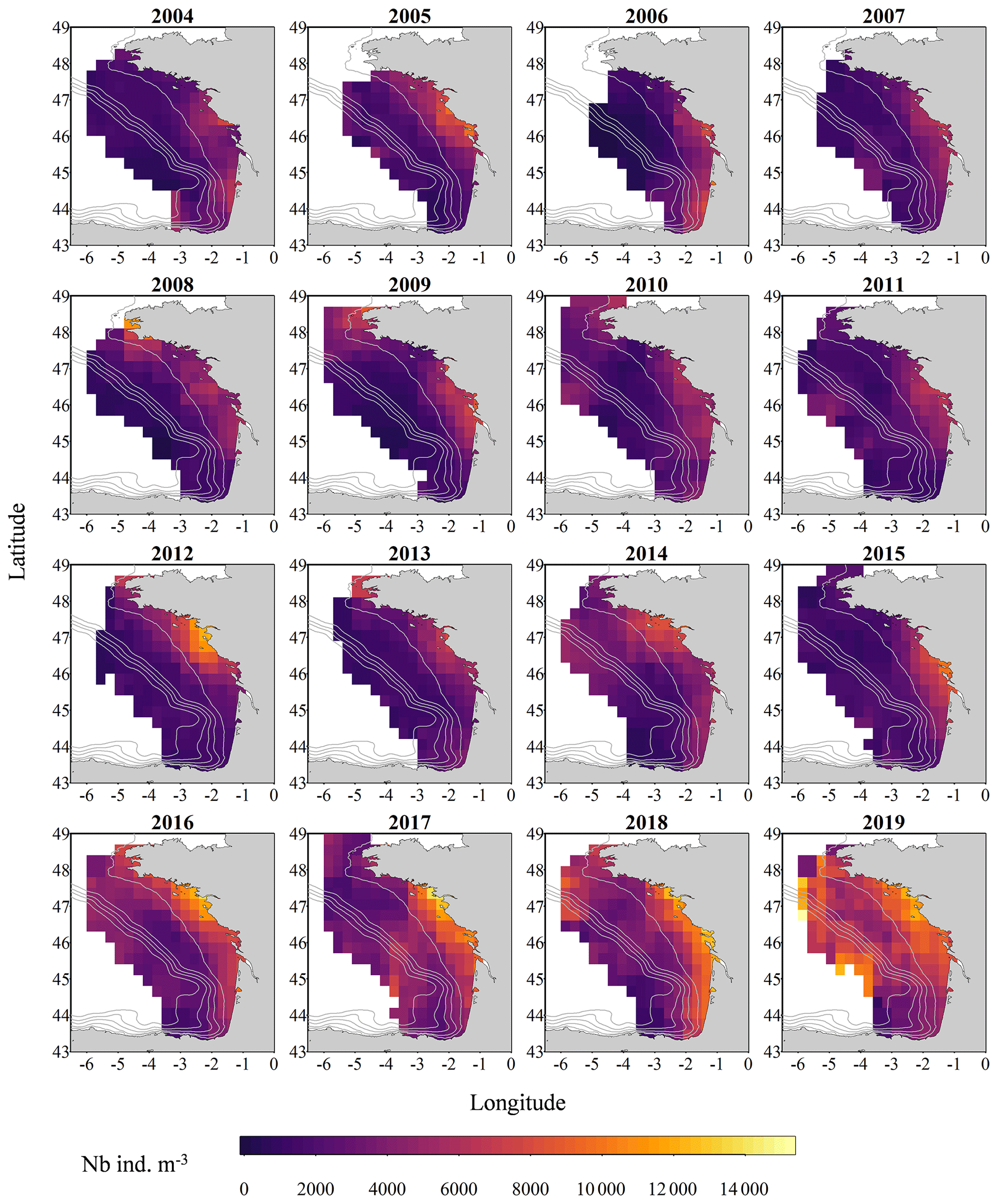
Figure 2 Gridded maps of total zooplankton abundances (expressed in individuals per cubic metre of sampled seawater) during the PELGAS cruises in the Bay of Biscay from 2004 to 2019. The abundances are well within the range of zooplankton abundances seen over other temperate continental shelves. They exhibit a marked coastal to offshore gradient, with abundances being higher at the coast. Abundances also show an overall increase over the years. The gridding procedure is presented in Petitgas et al. (2009, 2014). See also Doray et al. (2018c) and Grandremy et al. (2023a) for application examples.

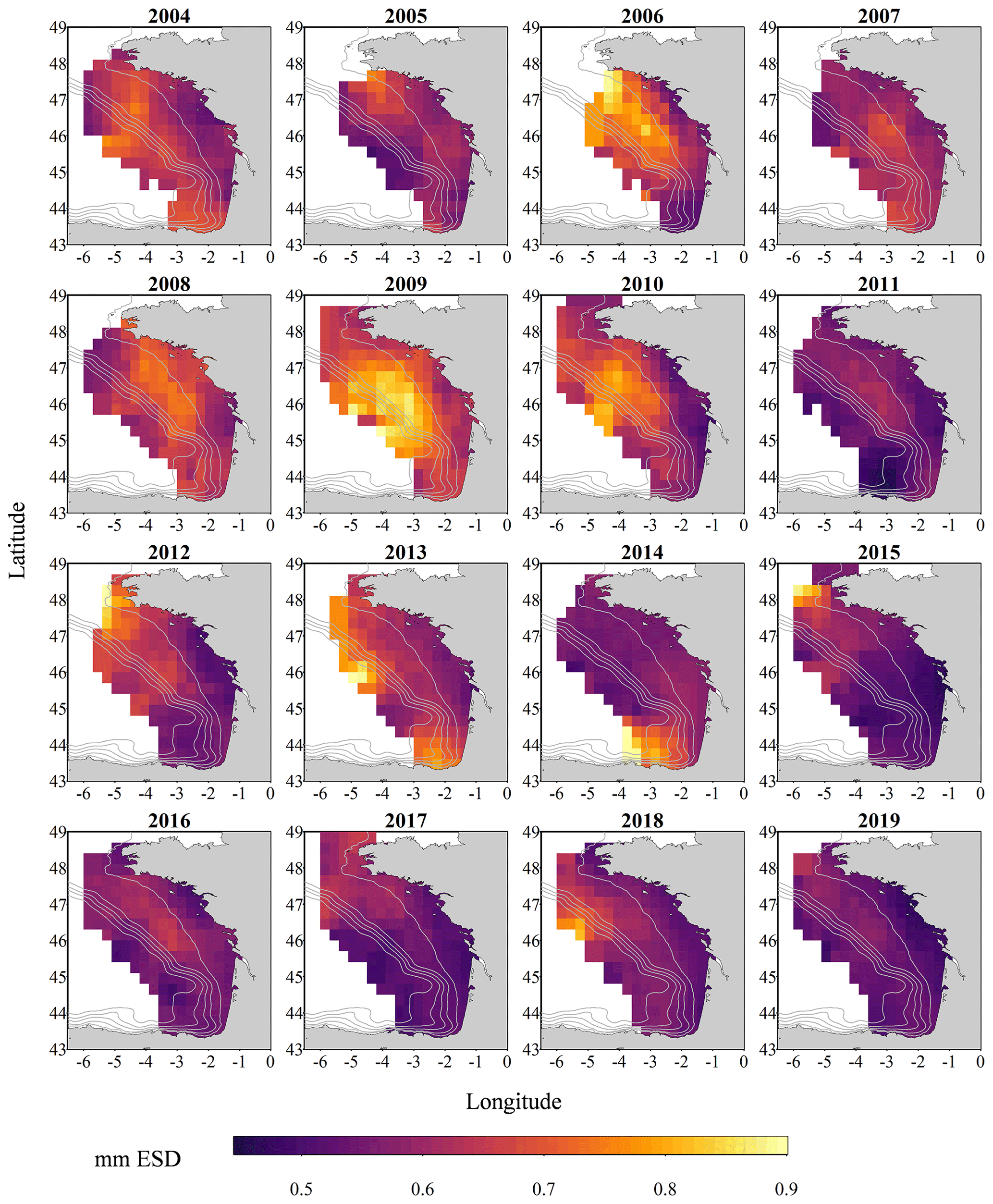
Figure 3 Gridded maps of total zooplankton mean size (expressed in mm equivalent spherical diameter) during the PELGAS cruise in the Bay of Biscay from 2004 to 2019. They exhibit a coastal to offshore gradient as well as a north–south gradient. Mean body sizes are smaller at the coast and usually smaller in the south. In general, mean body sizes show an overall decrease over the years. The gridding procedure is presented in Petitgas et al. (2009, 2014). See also Doray et al. (2018c) and Grandremy et al. (2023a) for application examples.

3 Datasets

3.1 Taxonomic groups and operational morphological groups

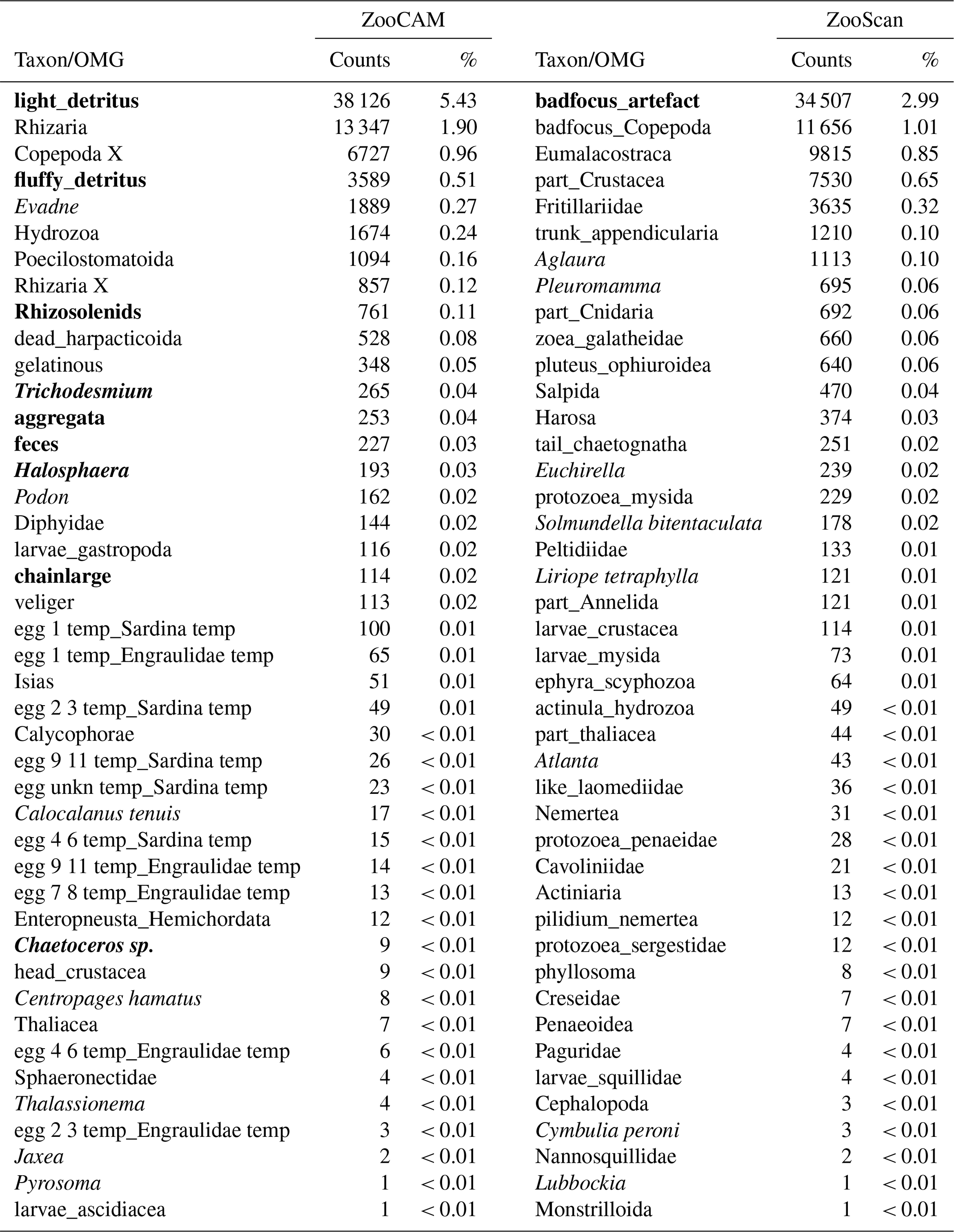
The ZooScan dataset is composed of 1 153 507 zooplankton individuals, zooplankton parts, non-living particles and imaging artefacts individually imaged and measured with the ZooScan and ZooProcess (Gorsky et al., 2010) and sorted into 127 taxonomic and morphological groups. The ZooCAM dataset is composed of 702 111 zooplankton individuals, zooplankton parts, non-living particles and imaging artefacts individually imaged and measured with the ZooCAM (Colas et al., 2018) and sorted into 127 taxonomic and morphological or life-stage groups. The total number of different groups identified with both instruments combined is 170, among which 84 are common to both datasets (Table 1), 43 belong to the ZooScan dataset only and 43 others belong to the ZooCAM dataset only (Table 2). The identified groups were divided into actual taxa and operational morphological groups (OMGs). Typically, OMGs are either non-adult life stages of taxa, aggregated morphological groups, or non-living groups (see Tables 1 and 2). Among the groups common to both instruments, 45 are actual taxa and 39 are OMGs (Table 1). Among the ZooScan-only groups, 22 are taxa and 21 are OMGs, and among the ZooCAM-only groups, 18 are taxa and 25 are OMGs (Table 2).

The differences in identified groups, in the taxa/OMGs ratio and in the associated counts arose from several aspects of the data generation. Firstly, the two imaging methods differ in their technical set-up. The main difference is that, on the one hand, fixed organisms are laid down and arranged manually on the imaging sensor and digitized in a lab (i.e. steady 2-D) set-up when using the ZooScan, whereas organisms are imaged live in a moving fluid in a 3-D environment (the flow cell) onboard when digitized with the ZooCAM. Their position in front of the camera may not enable an identification as precise as that achieved when they are laid on the scanner tray (Grandremy et al., 2023b; Colas et al., 2018). Secondly, the datasets are sequential in time: the ZooCAM dataset follows the ZooScan's. Zooplankton communities in the Bay of Biscay may have changed over time, even if their biomass as aggregated groups shows remarkable space-time stability (Grandremy et al., 2023a). Thirdly, we cannot guaranty that there is no adverse effect on taxonomic identification, as validation involved several experts (Culverhouse, 2007). Although we paid great attention to homogenizing the final detailed datasets, we recommend that taxa and OMGs should be aggregated and the biological resolution should be reduced for ecological studies (Grandremy et al., 2023a, b). Additionally, numerous identified and sorted taxa and OMGs do not belong to the metazoan zooplankton or they are non-adult life stages or parts of organisms. Those were included in the presented datasets because they are always found in natural samples. They need to be separated from entire organisms to ensure that abundance estimations are as accurate as possible, and they must be taken into account to ensure accurate biovolume or biomass estimations. A good example is the siphonophore issue: numerous swimming bells of degraded siphonophore individuals can be found and imaged in a sample. Determining an accurate siphonophore abundance may not be easy, but this could be overcome by considering the biovolume or biomass of siphonophores by adding up the biovolumes or biomasses of the numerous parts of the organisms imaged.

Table 1 Taxa and operational morphological groups (OMGs) common to the ZooCAM and ZooScan datasets. Taxa are listed on the left of the table and OMGs are listed on the right of the table. OMG names are spelled as they appear in the datasets. The numbers next to each taxon and OMG are the count and the percentage (%) for each category for each instrument in the whole dataset. Non-zooplanktonic OMGs are highlighted in bold, and genera and species are formatted in italics.

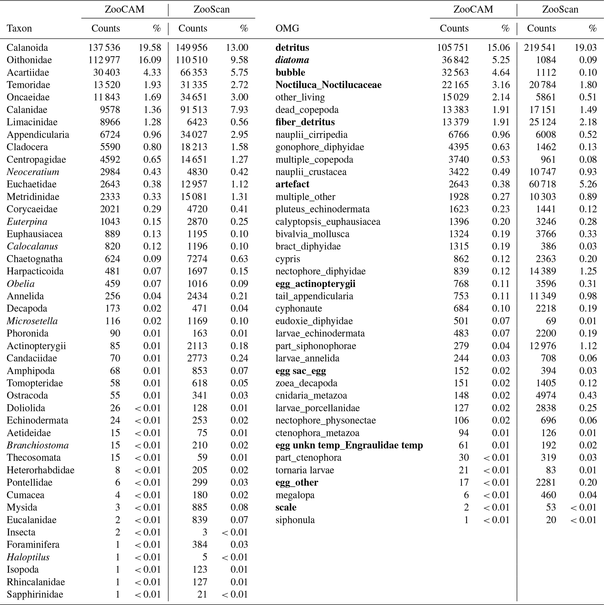
Table 2 Taxa and operational morphological groups (OMGs) present in either the ZooCAM dataset or the ZooScan dataset but not both. Taxa and OMGs appearing exclusively in the ZooCAM dataset are listed on the left; those appearing exclusively in the ZooScan dataset are listed on the right. OMG names are spelled as they appear in the dataset. The numbers next to each taxon and OMG are the count and the percentage (%) for each category for each instrument in the whole dataset. Non-zooplanktonic taxa and OMGs are highlighted in bold, and genera and species are formatted in italics.

OMG names mainly take the form of two words separated by “_” (underscore). Although we tried to name them as explicitly as possible, a few potentially needed clarifications can be found in Table 3.

Table 3 Non-exhaustive list of OMG prefixes, their types (morphological, developmental stage, taxonomic, non-living, or imaging artefact) and their contents.

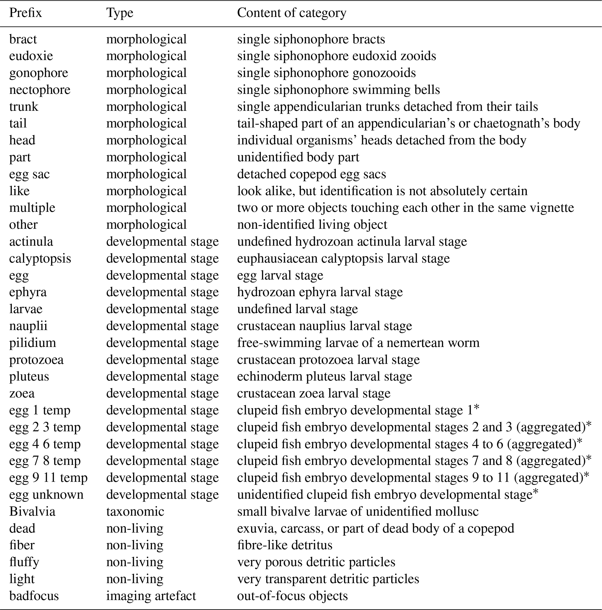
^* Clupeid fish embryo developmental stages according to Ahlstrom (1943) and Moser and Ahlstrom (1985).

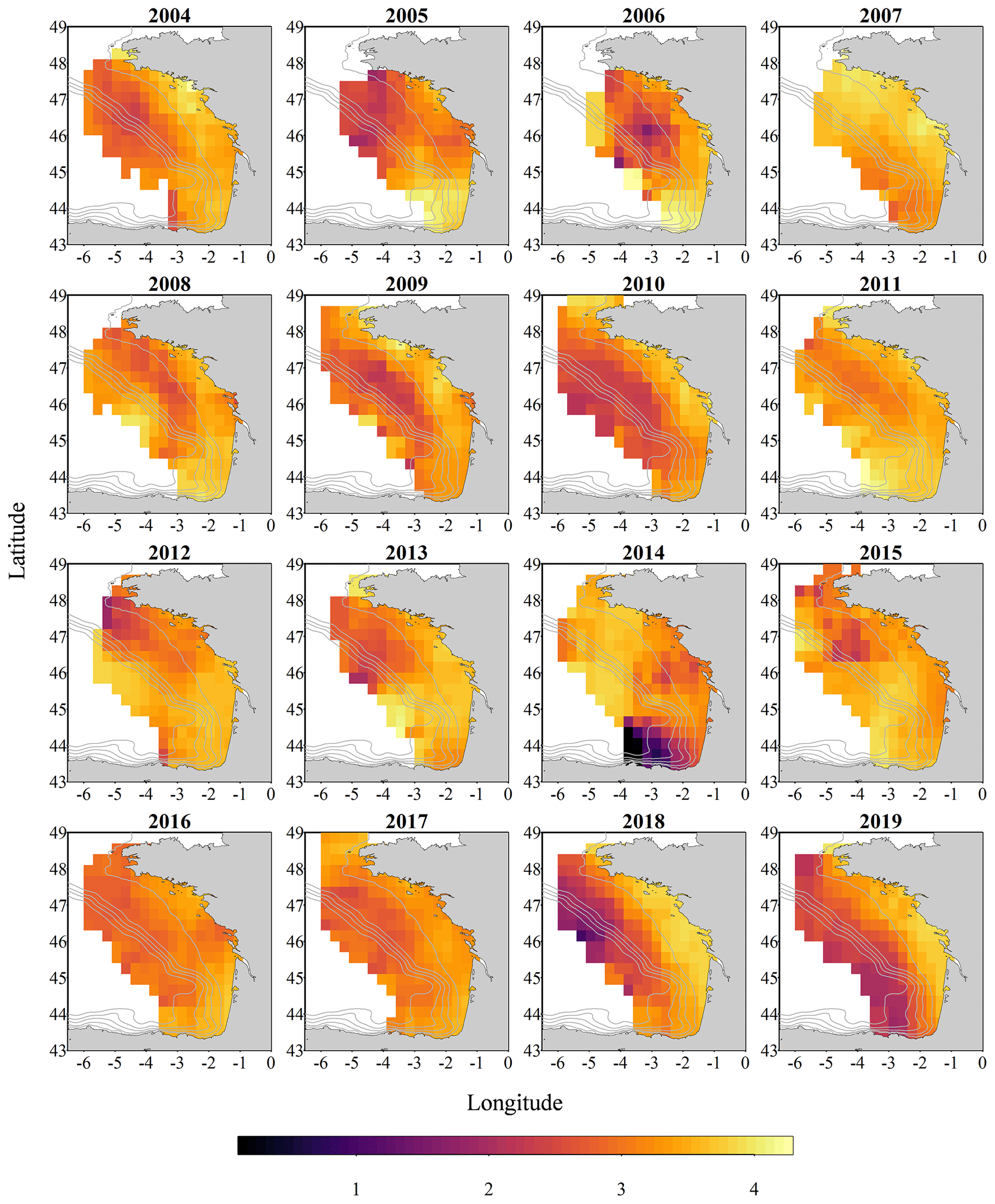
Figure 4 Gridded maps of total zooplankton Shannon index (calculated on spherical biovolumes) during the PELGAS cruise in the Bay of Biscay from 2004 to 2019. The Shannon index exhibits a coastal to offshore gradient as well as a north–south gradient. The Shannon index is larger at the coast and in the south except in 2014, where it is smaller offshore and in the south. The gridding procedure is presented in Petitgas et al. (2009, 2014). See also Doray et al. (2018c) and Grandremy et al. (2023a) for application examples.

3.2 Data and images

3.2.1 Data

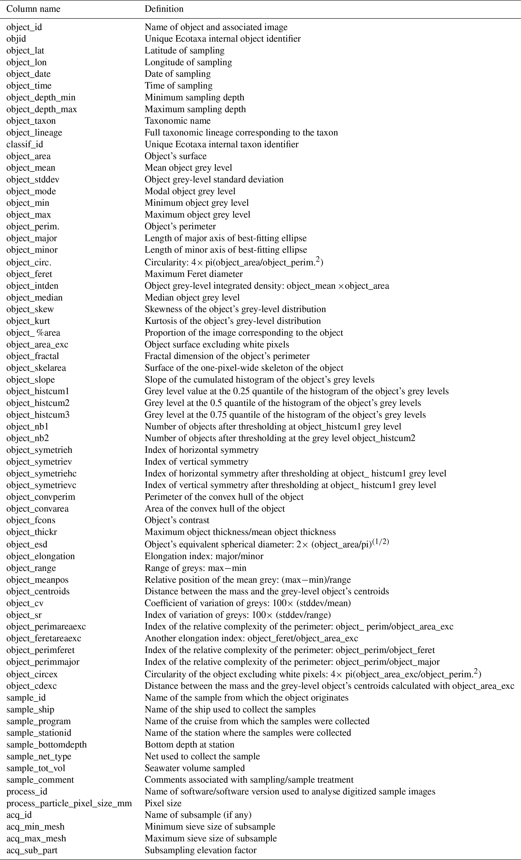
The data are divided into two datasets available as tab-separated files, one for each instrument. Within each dataset, the data is organized as a table containing text data as well as numerical data. Each dataset contains a combination of actual data and metadata at individual-object granularity. For each object, the user can find descriptors originating from the image processing (i.e. features), sampling metadata (i.e. latitude and longitude of the sampling station, date and time of sampling, sampling device, etc.), and sample processing metadata (i.e. subsampling factor, seawater sampled volume, pixel size) in columns and individual objects in lines. The column headers are defined in Tables A1 and A2 for the ZooCAM and ZooScan datasets respectively. The following prefixes enable the segregation of types of data and metadata: (i) “object_”, which identifies variables assigned to each object individually; (ii) “sample_”, which identifies variables assigned to each sample; (iii) “acq_”, which identifies variables assigned to each data acquisition for the same sample (note that this type of variable is only found in the ZooScan dataset, as ZooScan samples were split into two size fractions corresponding to two acquisitions); and (iv) “process_”, which identifies variables describing key image processing features (i.e. pixel size). Those prefixes originate from the use of the Ecotaxa web application to sort and identify the images (Picheral et al., 2017), which promotes this specific formatting. The ZooCAM dataset is arranged as a matrix with 72 columns (variables) × 702 111 rows (individual imaged objects), and the ZooScan dataset is arranged as a matrix with 71 columns (variables) × 1 153 507 rows (individual imaged objects).

Among the 70+ variables, it is worth noting the following ones:

• i.

  objid: this is a unique individual object numerical identifier that enables a single data line to be linked to a corresponding single image in the image dataset.

• ii.

  taxon: this is the taxonomic or OMG identification of the imaged objects, written as they appear in Tables 1 and 2.

• iii.

  lineage: this is the full taxonomic lineage of the taxon. Lineage may be used to aggregate taxa at higher taxonomic levels (respecting taxonomic lineages).

• iv.

  classif_id: This is a unique numerical taxon identifier.

• v.

  sample_sub_part/acq_sub_part: these are the subsampling ratios for ZooCAM and ZooScan respectively, which are needed to reconstruct the quantitative estimates of the sample abundances.

• vi.

  sample_fishingvolume/sample_tot_vol: these are the total sampled seawater volumes for ZooCAM and ZooScan respectively, which are needed to normalize the sample concentrations by the seawater volume.

One can therefore calculate quantitative abundance estimates for a taxon in a sample as follows:

$$\begin{array}{}\text{(1)}& {\displaystyle }\text{ZooCAM:}{\mathrm{Ab}}_{\mathrm{taxon}}={\displaystyle \frac{n_{\mathrm{taxon}}\times \text{sample\_sub\_part}}{\text{sample\_ fishingvolume}}}\text{(2)}& {\displaystyle }\begin{array}{rl}& \text{ZooScan:}{\text{Ab}}_{\text{taxon}}=\\ & {\displaystyle \frac{\left(n_{{\text{taxon}}_{\text{acq1}}}\times {\text{acq\_sub\_part}}_{\text{acq1}}\right)+\left(n_{{\text{taxon}}_{\text{acq2}}}\times {\text{acq\_sub\_part}}_{\text{acq2}}\right)}{\text{sample\_tot\_vol}}},\end{array}\end{array}$$

where Ab is the abundance in ind m⁻³ and n is the number of individuals for “taxon”.

3.2.2 Images

There are two sets of individual images sorted into folders by category (Tables 1 and 2) in each dataset. For the ZooCAM only, the images from years 2016 and 2017 contain printed region of interest (ROI) bounding-box limits and text at the bottom of each image and a non-homogenized background within and around the ROI bounding box; images from year 2018 contain a non-homogenized background within the ROI bounding box only; and images from 2019 have a completely homogeneous and thresholded background around the object. These differences arose from successive ZooCAM software updates that did not modify the calculation of an object's features. The ZooScan images all have a completely homogeneous and thresholded background around the object, with no bounding-box limits nor text printed in the images. All images for the two instruments' datasets have a 1 mm scale bar printed at the bottom left corner.

4 Data availability

The ZooScan dataset can be found as the PELGAS Bay of Biscay ZooScan zooplankton Dataset (2004–2016) at the SEANOE data portal at https://doi.org/10.17882/94052; Grandremy et al., 2023c). Individual object images can be freely viewed and explored by anyone using the Ecotaxa web application (https://ecotaxa.obs-vlfr.fr/, Picheral et al., 2017; no registration): search for the project name “PELGAS Bay of Biscay ZooScan zooplankton Dataset (2004–2016)” under the tab “explore images”.

The ZooCAM dataset can be found as the PELGAS Bay of Biscay ZooCAM zooplankton Dataset (2016–2019) at the SEANOE data portal (https://doi.org/10.17882/94040; Grandremy et al., 2023d). Individual object images can be freely viewed and explored by anyone using the Ecotaxa web application (https://ecotaxa.obs-vlfr.fr/; no registration): search for the project name “PELGAS Bay of Biscay ZooCAM zooplankton Dataset (2016–2019)” under the tab “explore images”.

Each dataset comes as a .zip archive that contains

• one tab-separated file containing all data and metadata associated with each imaged and identified object

• one comma-separated file containing the name, type, definition and unit of each field (column)

• one comma-separated file containing the taxonomic list of the dataset with counts and the nature of the content of the category

• a directory named individual_images containing images of individual objects that are named according to the object id objid and sorted into subdirectories according to taxonomic identification, year and sampling station.

5 Concluding remarks

Recent studies showed that small pelagic fish (SPF) communities have suffered from a drastic loss of condition in the Mediterranean Sea and in the Bay of Biscay (Van Beveren et al., 2014; Doray et al., 2018d; Saraux et al., 2019) over the last 20 years. This loss of condition is expressed in particular as a constant decrease in SPF size- and weight-at-age (Doray et al., 2018d; Véron et al., 2020) and is possibly explained by a change in SPF trophic resource composition, size and quality (Brosset et al., 2016; Queiros et al., 2019; Menu et al., 2023). Identifying and measuring zooplankton at appropriate temporal and spatial scales is not an easy task, but it can be addressed with imaging. These datasets were assembled in an effort to make possible the exploration of the relationship between the observed dynamics of SPF in the Bay of Biscay and the dynamics of their main food resource, metazoan zooplankton. This zooplankton imaging data series is a significant output of Nina Grandremy's PhD (2019–2023), and is currently being exploited (Grandremy et al., 2023a), and the intention is to continue this series and update it on a yearly basis in the framework of the PELGAS program to better understand the underlying processes presiding over the long-term SPF dynamics. Moreover, those two zooplankton datasets can be associated with the PELGAS survey datasets published in 2018 (which can also be found at the SEANOE data portal), which feature hydrological, primary producers, fish and megafauna data arranged as gridded data (Doray et al., 2018b). Together, all these datasets allow all of the pelagic ecosystem compartments to be studied simultaneously with a coherent spatial domain (the Bay of Biscay continental shelf), resolution and time series. Nevertheless, spatial gridding of the data is highly recommended (as presented in Figs. 2, 3 and 4), since the spatial coverage of the sampling protocols can vary between years (Fig. 1) within and between each pelagic ecosystem compartment. A procedure for such batch data spatial smoothing is presented in, for example, Petitgas et al. (2009, 2014). See also Doray et al. (2018c) and Grandremy et al. (2023a) for application examples. As several descriptors of the spring zooplankton community (abundances, sizes, biovolumes, biomass) can be derived from this 16-year-long spatially resolved time series at several taxonomic levels, these datasets are intended to be used in various ecological studies that include the zooplankton compartment, especially in modelling studies, where zooplankton is usually underrepresented (Mitra, 2010; Mitra et al., 2014). Finally, these datasets could also be applied as learning datasets when machine learning is used in plankton studies.

Appendix A

Table A1 ZooCAM dataset column headers – definitions of data and metadata fields.

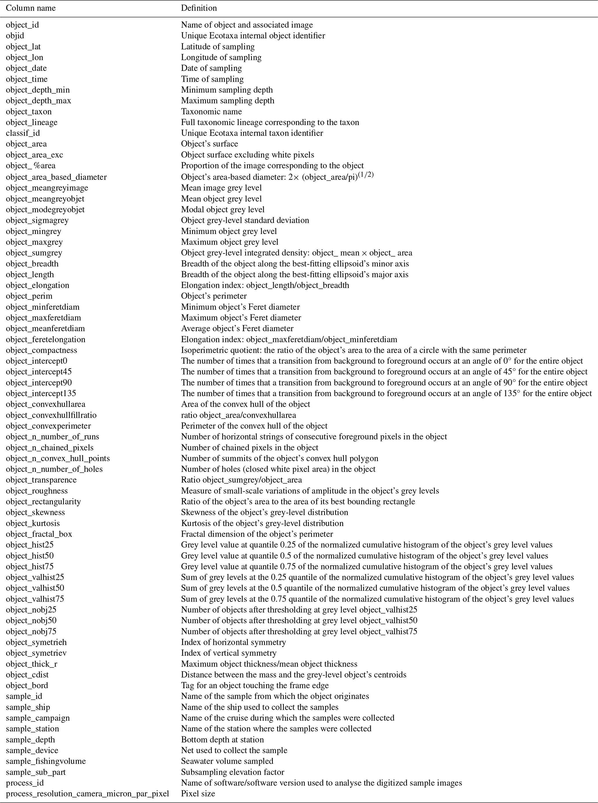
Table A2 ZooScan dataset column headers – definitions of data and metadata fields.