the Creative Commons Attribution 4.0 License.
the Creative Commons Attribution 4.0 License.
 | 12 Mar 2024
Mapping of sea ice concentration using the NASA NIMBUS 5 Electrically Scanning Microwave Radiometer data from 1972–1977
Rasmus T. Tonboe
Julienne Stroeve
The Electrically Scanning Microwave Radiometer (ESMR) instrument onboard the NIMBUS 5 satellite was a one-channel microwave radiometer that measured the 19.35 GHz horizontally polarized brightness temperature (TB) from 11 December 1972 to 16 May 1977. The original tape archive data in swath projection have recently been made available online by the NASA Goddard Earth Sciences Data and Information Services Center (GES DISC). Even though the ESMR was a predecessor of modern multi-frequency radiometers, there are still parts of modern processing methodologies which can be applied to the data to derive the sea ice extent globally.
Here, we have reprocessed the entire dataset using a modern processing methodology that includes the implementation of pre-processing filtering, dynamical tie points, and a radiative transfer model (RTM) together with numerical weather prediction (NWP) for atmospheric correction. We present the one-channel sea ice concentration (SIC) algorithm and the model for computing temporally and spatially varying SIC uncertainty estimates. Post-processing steps include resampling to daily grids, land-spillover correction, the application of climatological masks, the setting of processing flags, and the estimation of sea ice extent, monthly means, and trends. This sea ice dataset derived from the NIMBUS 5 ESMR extends the sea ice record with an important reference from the mid-1970s. To make it easier to perform a consistent analysis of sea ice development over time, the same grid and land mask as used for EUMETSAT's OSI-SAF SMMR-based sea-ice climate data record (CDR) were used for our ESMR dataset. SIC uncertainties were included to further ease comparison to other datasets and time periods.
We find that our sea ice extent in the Arctic and Antarctic in the 1970s is generally higher than those available from the National Snow and Ice Data Center (NSIDC) Distributed Active Archive Center (DAAC), which were derived from the same ESMR dataset, with mean differences of 240 000 and 590 000 km2, respectively. When comparing monthly sea ice extents, the largest differences reach up to 2 million km2. Such large differences cannot be explained by the different grids and land masks of the datasets alone and must therefore also result from the differences in data filtering and algorithms, such as the dynamical tie points and atmospheric correction.
The new ESMR SIC dataset has been released as part of the ESA Climate Change Initiative (ESA CCI) program and is publicly available at https://doi.org/10.5285/34a15b96f1134d9e95b9e486d74e49cf (Tonboe et al., 2023).
- Article
(7208 KB) - Full-text XML
- BibTeX
- EndNote


Several sea ice concentration (SIC) algorithms have been developed for passive microwave data (PMW). They differ in the usage of, e.g., frequencies and polarizations of the PMW data (Comiso et al., 1997) or the usage of static or dynamic tie points (Parkinson et al., 2004; Tonboe et al., 2016; Lavergne et al., 2019). From the resulting datasets, it is apparent that the Arctic sea ice extent (SIE) in September has been decreasing at a rate of about 12 % per decade since the launch of modern satellite multi-frequency microwave radiometers in 1978 (Onarheim et al., 2018; Stroeve and Notz, 2018). This negative sea ice trend in the Northern Hemisphere started in the 1970s (Rayner et al., 2003; Walsh et al., 2017), though regional trends can differ, as seen for example within the Barents Sea (Chapman and Walsh, 1991). In the Antarctic there are large regional differences in SIE trends, but, until recently, the overall trend was positive due to sea ice dynamics (Turner et al., 2009; Sun and Eisenman, 2021). This has changed, however, in the last decade as a result of several record lows, and, as such, overall trends have shifted to a more homogeneous pattern (Schroeter et al., 2023) and are now slightly negative in summer, November to February (NDJF). Until recently, the slightly positive trend was believed to be part of the long-term natural variability that overshadowed the effects of global warming starting in the 1960s (Wang et al., 2019; Stammerjohn et al., 2008; Thompson and Solomon, 2002; Ferreira et al., 2015; Singh et al., 2019; Fogt et al., 2022). In order to fully understand the drivers of sea ice variability, extending the sea ice data record backwards in time is essential.
Globally, SIE information prior to the satellite data record came largely from ice charts and ship observations. While there have been efforts to include these data in long-term assessments of sea ice change, the data are typically provided at relatively coarse spatial and temporal resolutions (1° grid) (Walsh et al., 2019), interpolating in both time and space (Titchner and Rayner, 2014). Only satellite-based datasets offer the ability to cover both hemispheres at improved spatial and temporal resolutions and generally show consistency in processing methods (Lavergne et al., 2019). The SIC derived from NIMBUS 5 Electrically Scanning Microwave Radiometer (ESMR) data was previously processed by Parkinson et al., 2004. Here, we apply a new processing method that is comparable to the EUMETSAT/ESA CCI SIC record from 1978 and onwards (see Andersen et al., 2006; Tonboe et al., 2016). Compared to Parkinson et al. (2004), this method reduces atmospheric noise regionally over both ice and water surfaces and uses the pre-processed data to develop a SIC algorithm calibration that is effective in removing both instrument drift and offsets. Seasonal sea ice signature variations are removed by using dynamical tie points. Lastly, the algorithm calculates temporally and spatially varying uncertainty estimates. The ESMR SIC data are presented on the same grid and with the same masking as the EUMETSAT/ESA CCI record, which makes these two records directly comparable. This and the modern processing chain mentioned above warrant the reprocessing presented in this article.
In Sect. 2, the satellite and reanalysis data are described, including the formatting and initial filtering of the data. Section 3 introduces the radiative transfer model (RTM) used for the atmospheric correction, while Sect. 4 describes the dynamical tie points, the SIC algorithm with uncertainty estimations, the land-spillover method, and data flags assigned during post-processing. In Sect. 5, the resulting SIC dataset is presented and compared to other datasets. Finally, Sect. 6 consists of a discussion, and Sect. 7 provides the conclusions of this work.
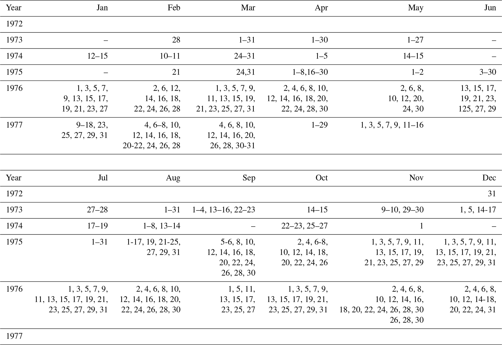
The NIMBUS 5 ESMR instrument was a cross-track scanner that measured at 78 scan positions perpendicular to the flight track with a maximum incidence angle of about 64° on both sides (NASA GSFC, 2016). No direct observations at nadir were made; the closest positions were at ±0.7°. Its near-circular orbit had a height of about 1112 km and an inclination of 81°. The phased-array antenna dimensions were 85.5×83.3 cm, and the spatial resolution was about 25 km near nadir, increasing to about 160×45 km at the edges of the swath (NASA GSFC, 2016). The full swath was about 3100 km, with the varying incidence angle and the spatial resolution giving very good (unprecedented) daily coverage in polar regions with no gaps, i.e., no pole holes. The ESMR onboard the NIMBUS 5 satellite was a one-channel 19.35 GHz horizontally polarized microwave radiometer operating from 11 December 1972 until 16 May 1977 (1617 d) with some interruptions (see the list of days with missing files in Appendix A2). Due to a hot-load anomaly, there are major data gaps between March to May and again in August 1973. Another major data gap occurs from 3 June until 14 September 1975 because the ground segment was used for receiving NIMBUS 6 data instead (Parkinson et al., 1999). When operation was resumed in September 1975, the instrument was only operated approximately every other day. From late 1976 to the end of the mission, operation was highly irregular. The last file in the dataset is from 16 May 1977. The data have recently been made available online by NASA in the original tape archive format (TAP files).
2.1 Formatting and co-location of brightness temperatures and ECMWF ERA5 data
The ESMR data were retrieved from the online data archive of the NASA Goddard Earth Sciences Data and Information Services Center (GES DISC) (NASA GSFC, 2016). This dataset contains, along with a number of instrument and geographical parameters, calibrated 19.35 GHz brightness temperatures expressed in units of kelvin. The raw data were recovered by NASA from the magnetic tapes, called calibrated brightness temperature tapes (CBTTs), where they were stored in the original binary TAP file format, each file corresponding to a particular orbit (NASA GSFC, 2016).
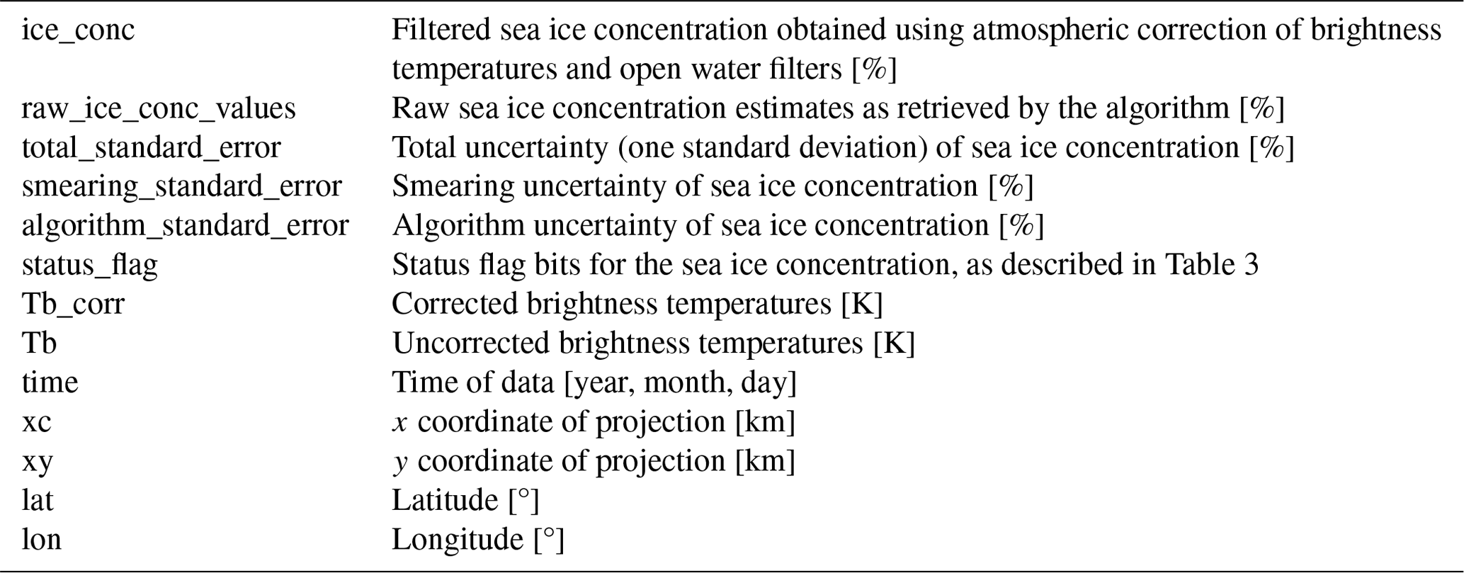
All variables in the TAP files were read using online NASA software and converted to NetCDF format without changing the original data structure, creating raw ESMR NetCDF files. Each data point in the TAP file was matched with the European Centre for Medium-Range Weather Forecasts (ECMWF) ERA5 re-analysis data (Bell et al., 2020; Hersbach et al., 2020) that were nearest in time and space and appended to the raw ESMR NetCDF file serving as input to the processing chain. The resulting data are structured in arrays line by line (across track). Appendix A1 summarizes the variables included in the NetCDF files.
2.2 Initial filtering and correction of brightness temperatures
NASA provides a correction of the brightness temperature data to account for the lobe structure, antenna loss, and angular brightness temperature (TB) variation (NASA CR, 1974). According to NASA, the correction was needed because “The cause of the gross variations in antenna properties which were observed soon after launch has been determined to be a cross-polarized grating lobe […] The problem does not exist for the near-nadir beam positions so these positions are unaffected. […] An empirical calibration has been developed which removes the effect of the lobe structure and antenna loss, which vary with position, and roughly corrects for angular variations in viewing geometry.” (NASA CR, 1974, p. 400).
Originally, it was planned to use only lobe-corrected TB values with their natural angular dependency, but we did not find a way to extract this from the NASA-provided dataset. Essentially, only the combined lobe and angular correction, which is a function of brightness temperature, can be removed altogether from the data NASA provides. Thus, the TB values do not vary as a function of incidence angle, as would be expected for TB values from the sea surface and sea ice.
Despite the corrections done by NASA, the ESMR data still contain erroneous TB values, scan lines, sudden jumps in the calibration, and other obvious artifacts.
Since the ESMR data contain corrupted data and erroneous scan lines, filtering is needed before the data can be used for sea ice mapping. The filters that we apply are described in Eqs. (1)–(4). They are applied in the same order as described here. If only a single data point or a couple of scan lines are affected, only those data points and scan lines are removed from the file. If the whole file is corrupted then it is deleted.
An initial analog filter is used for filtering erroneous TB values and scan lines. The filter is based on the 16 analog voltage entries in the data. The NIMBUS 5 ESMR user's guide (Sabatini, 1972) does not explain very well what the 16 entries really are, or what unit the voltages are stored in, but jumps in these analog signals correspond to anomalous TB values. Our analog filter computes the absolute gradient in the analog signals, and anything over a value of 10 is removed. This threshold was estimated experimentally.
Next, several other filters are employed using the processed TB (in K) from the previous step. The filters are applied in the following order.
Data that are non-physical and outside the expected range for sea and ice surfaces are removed. Only data points that lie inside the range specified in Eq. (1) are kept:
The next filter removes erroneous scan lines (across track rows). Consecutive scan lines should not differ by more than 50 K, as shown in Eq. (2). The threshold of 50 K was estimated experimentally.
where in Eq. (2) is an across-track row of TB values and i is an index along the track, while j is an index across the track. n is the maximum across-track index of a row, i.e., for a complete row with valid data points for all 78 incidence angles, n=78.
Afterwards, single TB outliers are removed if they do not satisfy Eq. (3):
where p is a single-pixel TB and i is an along-track index. The threshold of 150 K was selected manually after identifying erroneous single-pixel outliers in the data. The last filter in Eq. (4) removes neighboring TB values which are locked to the same value, i.e., TB values for which the following equation equals zero:
where p is again a single-pixel TB with an along-track index i. The decision to compare seven consecutive TB values was made based on qualitative experiments. Since the filter is used universally for all incidence angles, the search window varies but covers a minimum distance of 175 km.
The outer data points of the swath edges show significantly higher noise levels and a coarser resolution than the near-nadir data points (Veng, 2021). Therefore, after the filtering, we additionally remove the four outermost data points of the swath, corresponding to incidence angles between 57° and 64° on both sides. The new outer edge of the swath data is then at ∼56°, similar to that of modern microwave radiometers used for sea ice retrieval: 50–55° (AMSR, Meisner and Wentz, 2000; SMMR, Wentz, 1983; SSM/I, Wentz, 1997).
Before the filtering, the dataset contained 13 496 orbital data files; after filtering, there are 10 649 (∼79 %) good files left. A complete list of days where data are missing after filtering and no SIC could be retrieved is given in Appendix A3.
The radiative transfer model (RTM) was developed specifically for atmospheric noise reduction and is comparable to the RTMs used in Andersen et al. (2006) and Tonboe et al. (2016) but with the addition that this ESMR RTM (Eq. 5) can be applied for different incidence angles over both ocean and ice. The RTM takes as input the atmospheric columnar water vapor V [mm or kg m−2], the 10 m wind speed W [m s−1], the atmospheric columnar cloud liquid water L [mm or kg m−2], the sea surface temperature Ts [K], the ice emitting layer temperature Ti [K], the sea ice concentration cice [0–1], and the incidence angle [°]. In return, it simulates the top-of-the-atmosphere 19.35 GHz TB at horizontal polarization:
The RTM uses the atmospheric part of the model described in Wentz (1997) to compute the atmospheric emission, transmissivity, and reflectivity at the sea surface (open water) together with added modules for simulating the sea ice emissivity (Fig. 1) and open water reflectivity as a function of incidence angle.
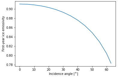
For the sea ice emissivity, a look-up table is produced from a simulation using a combined sea ice thermodynamic and emission model during the Arctic winter on first-year ice. The thermodynamical and emission model setup and the simulations are described in Tonboe (2010). The emissivities as a function of incidence angle are shown in Fig. 1, and the look-up table is given in Table 1.
Table 1Sea ice emissivity look-up table (θ is the incidence angle and Eice is the first-year ice emissivity).

Sea water permittivity, which is used to estimate the calm sea reflectivity (Eq. 6) as a function of temperature, is computed using equation E64 (p. 2046) in Ulaby et al. (1986). The permittivity is almost invariant with respect to the water salinity at 19 GHz, and a constant value of 34 ppt is used here.
The calm sea (Fresnel) power reflection coefficient, rh, as a function of the relative permittivity, ϵ, and the incidence angle, θ, for a lossy medium is computed using Eq. (1.52) in Schanda (1986), i.e.,
where p and q are abbreviations for:
and
The relative permittivity of the water surface is a complex number. The calm sea emissivity, E0, is then
The rough water surface emissivity component, EW, is added to the calm sea emissivity, E0, to produce the total sea water emissivity, Ewater. Between ESMR incidence angles of 0 and 63°, the sensitivity of the 19.35 GHz horizontal polarization, EW, to wind speed is an almost linear function of the incidence angle θ (Meisner and Wentz, 2012), i.e.,
and
where θ is the incidence angle in degrees, W is the wind speed, and Ts is the sea surface temperature [K].
This combination of E0 and EW follows the procedure described in Wentz (1997).
The resulting brightness temperature is a linear combination of the sea water and sea ice emission weighted by the SIC following Andersen et al. (2006):
where TBU is the upwelling brightness temperature from the atmosphere, τ is the atmospheric transmissivity, Ewater is the water surface emissivity, Eice is the sea ice emissivity, Ω is the reflection reduction factor due to water surface roughness, TBD is the downwelling brightness temperature, and TBC is the cosmic background brightness temperature (2.7 K).
EMSR-simulated TB values and emissivities have been compared with other TB values simulated using other RTMs for AMSR (Meisner and Wentz, 2000), SMMR (Wentz, 1983), and SSM/I (Wentz, 1997) for a constant incidence angle of 55°, which is close to the incidence angles of other instruments and RTMs (53–55°). The comparison showed that the TB values of the ESMR RTM are within the range (within approx. 2 K) of values obtained with the other models and therefore seem to be reasonable given the differences in instrument center frequencies and measurement geometries. Note that in the correction procedure, the difference between two simulated TB values is used to minimize model biases. Even if the absolute values of the RTM-simulated TB values were biased, this bias would be removed by taking the difference between two simulated TB values, which is the only part used in the correction.
The RTM is an essential part of the SIC derivation for applying an atmospheric noise reduction. The following section presents the calculations of dynamical tie points and the SIC algorithm along with uncertainty estimations. Lastly, the post-processing, including the land-spillover method and data flag assignment, is described. A flow chart illustrating this processing chain can be found in the ESA CCI ESMR product user guide (PUG) (ESA CCI, 2022).
4.1 Tie points and geophysical noise reduction
Tie points are typical signatures of 100 % ice and open water (0 % ice) and are used in SIC algorithms as a reference for estimating the total ice fraction per satellite pixel cice. The aim of using dynamical tie points is to reduce SIC biases that may result from seasonal and interannual variations in TB (Kongoli et al., 2011), instrument drift, and RTM and ERA5 biases. For example, Comiso and Zwally (1980) argue that the variations in the average open-water TB values near the ice edge are affected primarily by variations in instrument calibration, and they describe the drop followed by a sharp increase seen in 1975 (see Fig. 2) as an instrument drift issue.
Our ESMR tie points are derived on a daily basis from the swath files. Regions of open water and high SICs are selected for each hemisphere, resulting in two regions of sea ice and two of open water for both hemispheres. The ERA5 SIC prior to 1979 is based on the HadISST2.0.0.0 dataset (Bell et al., 2021), which mainly utilizes digitized sea ice charts for this period (Rayner et al., 2003). The two main data sources are the Walsh dataset (Walsh, 1978; Walsh and Johnson, 1979; Walsh and Chapman, 2001) and National Ice Center (NIC) charts (Knight, 1984). The datasets also consist of several data types besides ice charts, e.g., ship observations and satellite data (both infrared and microwave observations, including data from ESMR). The selection of the four tie points is based on a criteria set for SIC from ERA5 – the distance from the ice edge, the observed brightness temperature, the latitude, and the sea surface temperature – as shown in Table 2. The distance from the ice edge criterion is imposed by putting a threshold on the mean SIC of a 5×5 grid point box; this should be larger than 80 % for ice tie points or less than 1 % for open water points. While computed daily, these are subsequently combined into 15 d running-mean tie points that are 7 d ahead and 7 d behind the processed date shown in Fig. 2. The 15 d averaging period is maintained even at the beginning and end of the dataset and when there are data gaps; i.e., if there are gaps, the averaging is done over the days available in the 15 d period (this is also the case in the beginning, where the first 7 d are missing). Figure 2 depicts the 15 d averaged tie points through time. It shows that the ice tie points follow a seasonal pattern, while the water tie points are relatively constant. The tie-point criteria from Table 2 ensure that each daily tie point is based on many observations, which results in stable tie points. The 15 d interval was chosen experimentally, so the TB variations seem reasonable and one is still able to identify calibration issues such as jumps (e.g., that seen in 1976).
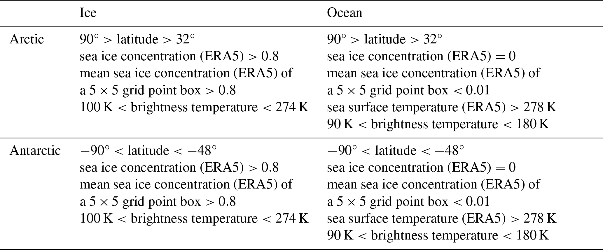
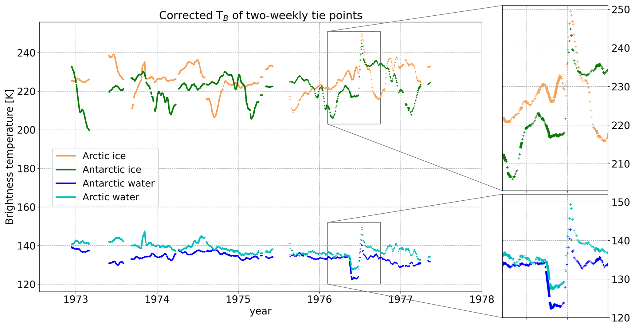
Figure 2The 2-weekly tie points for Arctic and Antarctic ice and water after TB correction. The boxes show the period May–July 1976, when there were obvious instrument calibration issues.
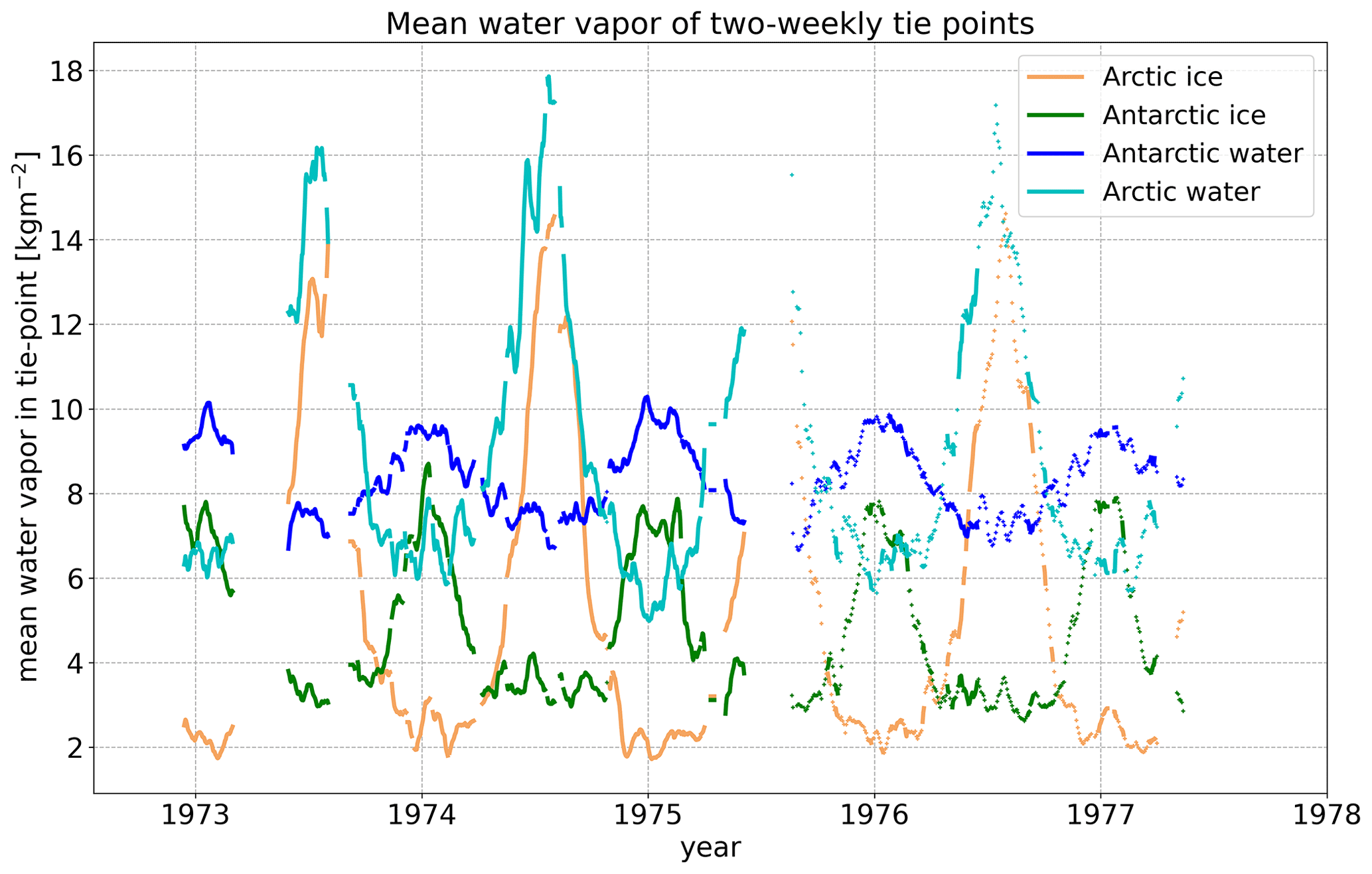
Figure 3Mean atmospheric water vapor for all grid points included in the four tie points. Water vapor data are from ERA5 (Hersbach et al., 2020).
The per-grid-point TB correction term ΔTB,simulated is the difference between a simulated reference TB obtained using mean values of the total column water vapor [kg m−2] in the atmosphere (), 10 m wind speed [m s−1] (), total column cloud liquid water [kg m−2] in the atmosphere (), sea surface temperature (), and ice emitting layer temperature () as input to the RTM and a simulated TB obtained using the actual ERA5 values (V, W, , Ts, and Ti) for the grid point. TB is not corrected for the cloud liquid water, L, so the mean L is input to both the reference and the actual simulation. ΔTB,simulated can both be negative and positive, and the TB values have a reduced sensitivity to the geophysical noise sources (V, W, Ts, Ti) after correction. The fact that the correction term is the difference between two RTM simulations minimizes the impact of biases in the model and the ERA5 data.
The correction term is added to the measured TB, i.e.,
Here,
where cice=0 is the open water tie point and cice=1 the ice tie point. Following Svendsen et al. (1983), Ti is computed as
where T2 m is the 2 m air temperature, which is taken from the ERA5 data. Horizontal bars above the variables indicate that they are daily mean values for the cluster of points selected for the tie point. The mean water vapor, , at the tie point is shown in Fig. 3.
Figure 4 shows the correction term, ΔTB,simulated, for 1 January 1974 over open water in the Northern and Southern hemispheres, respectively. The path length through the atmosphere is longest at high incidence angles and shortest near nadir, and thus the absolute value of the correction is largest at high incidence angles. For example, when the atmosphere is driest in the reference compared to the actual simulation, the ends of the corrected TB turn negative, while they turn strongly positive when the reverse is true.
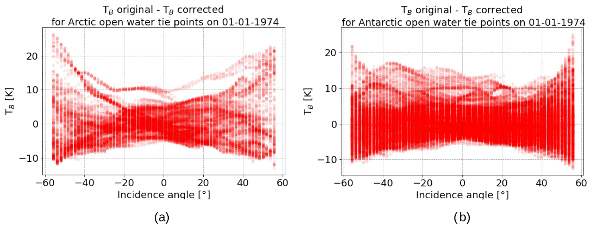
Figure 4Difference between the TB values before and after correction with a mean reference for open water tie points in the (a) Northern Hemisphere and (b) Southern Hemisphere.
The correction works best over open water areas, where it acts as only an atmospheric correction. The RTM appears to better simulate the relevant emission processes in the atmosphere, and the ERA5 data more accurately quantify the atmospheric noise sources. Over sea ice, geophysical noise sources are related to processes in the snow and ice profile (Tonboe et al., 2021) which are not characterized by the RTM, except for the emitting layer temperature Ti. Ti, which is used as input to the RTM, is estimated from the 2 m air temperature in the ERA5 data using Eq. (15). This is important because the ESMR is a single-channel instrument and thus the TB and also the derived cice are sensitive to the emitting layer temperature.
The standard deviations of the brightness temperature for water points in both hemispheres before and after the correction are shown in Fig. 5.
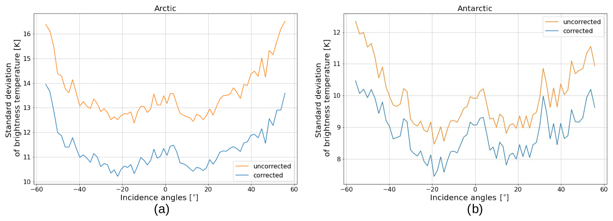
Figure 5Standard deviations of TB values before and after correction in January 1974 for the (a) Northern Hemisphere and (b) Southern Hemisphere. The plots only show ocean points which fulfill the ERA5 SIC and sea surface temperature (SST) criteria described in Table 2.
4.2 The sea ice concentration (SIC) and its uncertainty
SIC (cice) is estimated using the measured brightness temperature (TB,measured) and the open water (Tp,water) and ice (Tp,ice) tie points, i.e.,
Because the RTM requires cice as input, cice is processed iteratively in two steps:
-
The cice is first estimated using uncorrected TB values and tie points derived from uncorrected data. The cice estimate is truncated to the interval between 0 and 1 and an open water filter is applied, forcing all cice values of less than 0.15 to 0.
-
The cice estimate from step (1) is used in the RTM calculation (Eq. 5) together with ERA5 data for the geophysical noise reduction of the TB values, and cice is then estimated again in a second iteration, this time using the corrected TB values and corrected tie points. The mean values of used in the reference simulation are averages weighted by the cice obtained using the mean water and ice tie-point values respectively, i.e., cice is used as a ratio to mix the two tie-point values to create mean values of the numerical weather prediction (NWP) data for any sea ice concentration.
Iterations to update cice could continue in principle. However, tests show that updates are small after one iteration, and so we only iterate once (e.g., Lavergne et al., 2019).
The total SIC uncertainty is the combination of two components: (1) the algorithm uncertainty, which includes instrument noise and tie-point variability (geophysical noise), and (2) the resampling uncertainty, which is the uncertainty due to data resampling.
The algorithm uncertainty is the squared sum of three independent components following Parkinson et al. (1987):
where the first term in Eq. (17) represents variations due to instrument noise, estimated to a brightness temperature error δTB of 3 K (Parkinson et al., 1987).
Without the instrument noise term, which is already included in the two tie-point uncertainties, the second and third terms in Eq. (17) are used to compute the algorithm uncertainty, δcice,algorithm:
where δTp,water is the water tie-point error (1 standard deviation of the daily tie point here) and δTp,ice is the ice tie-point error (e.g., 1 standard deviation of the daily tie point). The water and ice tie-point errors are weighted by the SIC, and all three errors are normalized with the ice–water brightness temperature contrast and the 2-weekly tie points. The algorithm uncertainty is computed based on swath data.
The resampling uncertainty δcice,re-sampling is the maximum difference cice- minimum cice in a 3×3 pixel window. The resampling uncertainty is computed based on resampled data (e.g., Lavergne et al., 2019).
The total uncertainty is the squared sum of the algorithm and resampling uncertainties, i.e.,
The two uncertainty components and the total uncertainty are included in the data file.
4.3 Land-spillover correction and post-processing
The land-spillover correction follows the procedure described in Markus and Cavalieri (2009). A 5 by 5 pixel neighborhood of the land mask (EASE2 version 2, by OSI-SAF) is analyzed to determine which coastal points should be corrected. The land mask is divided into two classes: land points, which are given a value of 90 % SIC, and open ocean points. If the difference between the original land mask and the mean mask calculated for the 5 by 5 window is larger than the previously estimated SIC (the RTM-corrected and resampled SIC), i.e., the SIC is smaller than the theoretical value of the land spillover, the SIC value is set to 0 % and the status flag variable of the dataset is raised to 8.
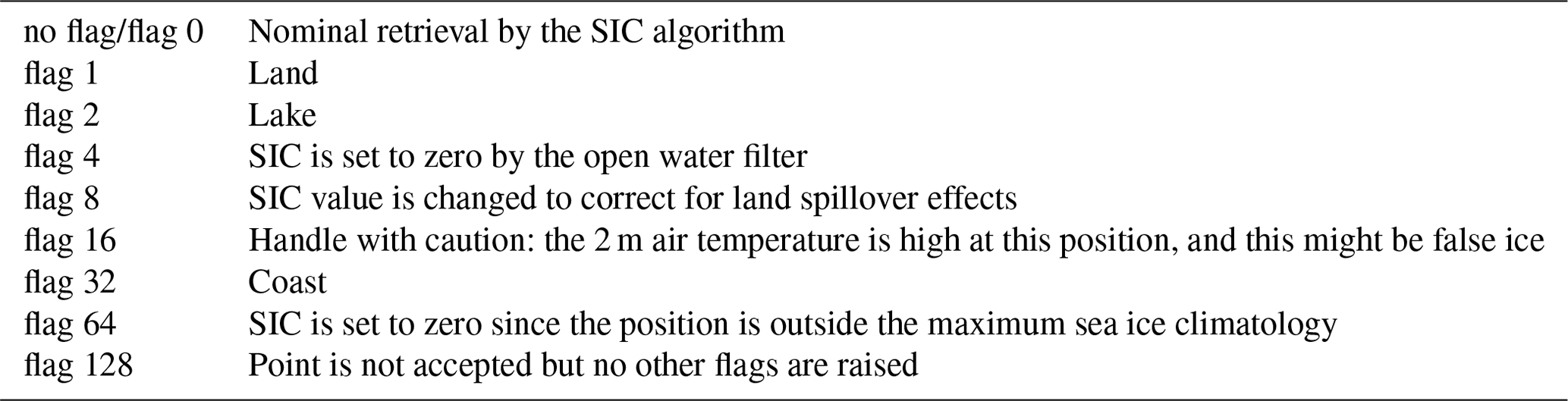
Additionally, a monthly climatology (also from OSI-SAF; the same version as for the land mask) is used to set SIC to 0 % and to mark open water points by a climatology boundary, which is indicated by a status flag value of 64. Afterwards, the land mask is also used to mark lakes and coastal areas with status flags 2 and 32, respectively. An overview of all status flag values is shown in Table 3.
Table 3Description of values of the status flag variable of the dataset.
The results of the post-processing are included in the daily NetCDF files for the Northern and Southern hemispheres, respectively.
A list of all output variables in the daily SIC files and a short description of them can be seen in Appendix A2. Examples of monthly means of the SIC and the mean uncertainty can be seen in Figs. 6 and 7.
It is worth noting that the coverage in Fig. 6 is complete and, because of the ESMR's wide swath width of 3100 km and its inclination, the North Pole is covered, in contrast to the satellite microwave radiometers that have followed the NIMBUS 5 ESMR, which have a “pole hole”. The area covered by multi-year ice in the central Arctic has a lower SIC than the first-year ice regions. This is a consequence of the one-channel SIC algorithm, which has inherent ambiguity in SIC, ice type, and emitting layer temperature variations. In Figs. 6b and 7b, it can be seen that the uncertainties are largest near the ice edges, as expected. This is due to the resampling uncertainty, which dominates near the ice edge, where the spatial variability of TB is high. Coastal regions also show higher uncertainties for this reason, since the land-spillover correction is first applied to the SIC after the uncertainty estimations.
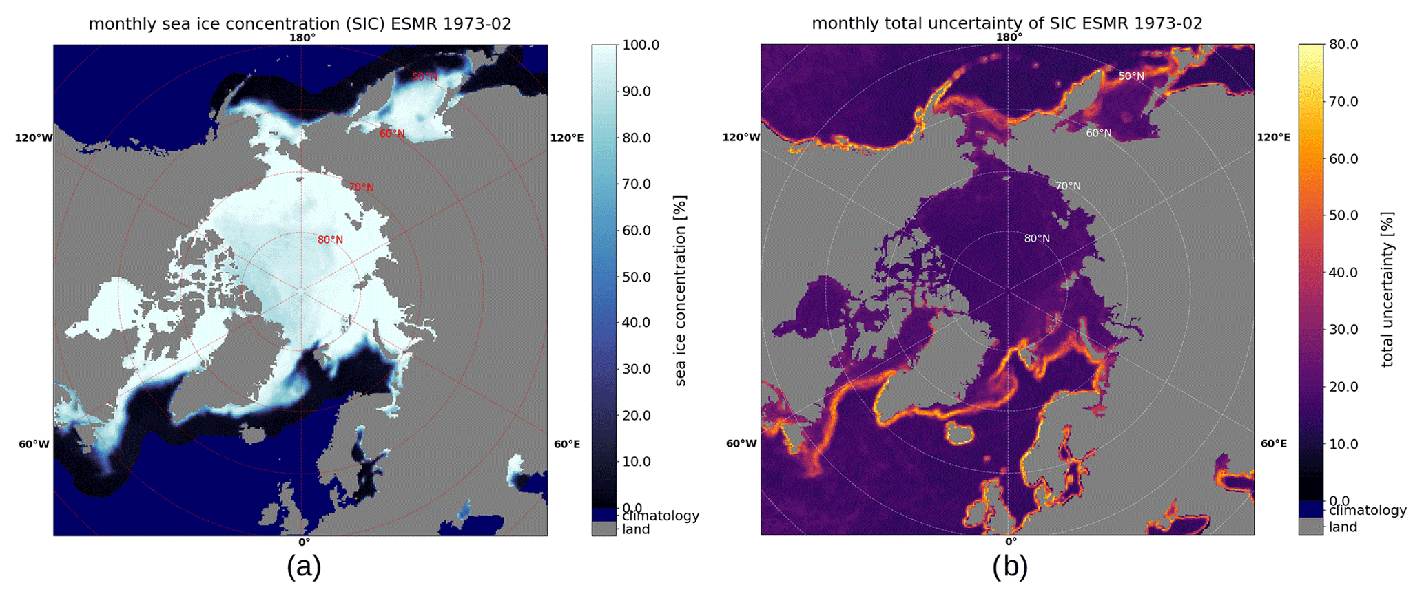
Figure 6Monthly mean (a) SIC and (b) uncertainty for February 1973 in the Northern Hemisphere. Water areas with no ice and uncertainty due to the ocean climatology are displayed in dark blue.
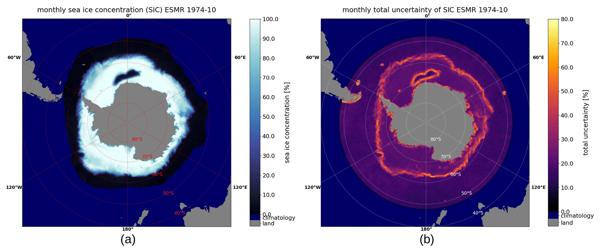
Figure 7Monthly mean (a) SIC and (b) uncertainty for October 1974 in the Southern Hemisphere. Water areas with no ice and uncertainty due to the ocean climatology are displayed in dark blue.
The SIC shows interesting sea ice features in the years 1972–1977. One such feature is the Odden ice tongue (Comiso et al., 2001) extending eastward from the East Greenland Current, which is visible in Fig. 6 (around 73° N, 0° E), while another feature is the Maud Rise Polynya (Jena et al., 2019), an open water area encircled by sea ice in the Southern Hemisphere, which can be seen in Fig. 7 (around 65° S, 0° E). Both examples were much larger in extent in the 1970s and occurred more frequently then than they do today (Comiso et al., 2001; Cheon and Gordon, 2019; Jena et al., 2019).
The daily coverage of valid data points that passed all filtering varied a lot through the ESMR's operating period. While there was nearly full coverage for the first few months, it got much worse after the summer of 1975, when the instrument only recorded data every second day. An example of the poor coverage is shown for May 1976 in Fig. 8.
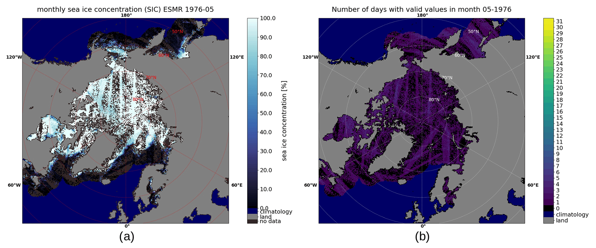
Figure 8Example of poor monthly coverage in May 1976 in the Northern Hemisphere for (a) the mean SIC and (b) the number of days with valid values. Water areas that showed full daily coverage due to the ocean climatology are displayed in dark blue to avoid misleading comparisons. The number of days with valid data is indicated by the colorbar.
Monthly averaged SICs are derived to compare our results against other datasets. Only months with 99 % coverage were used in the comparison, i.e., 99 % of all grid points are covered at least once per month. Monthly mean SIEs are calculated from the monthly SICs using the threshold cice>30 %. In Fig. 9, the ESMR dataset (orange line) is shown together with the OSI-SAF climate data record (CDR; blue line) for 1979–2022 (EUMETSAT, 2017a, b) and the sea ice extent derived from the NSIDC's NIMBUS 5 ESMR ice concentration product (green line) (Parkinson et al., 2004), using the same threshold for all products (cice>30 %).
The comparison shows comparable SIE levels around 1980. In general, our ESMR dataset has slightly higher monthly SIE values than the NSIDC's ESMR product, even though the seasonal pattern is the same.
The mean difference between our sea ice extent and that from NSIDC is 0.24 million km2 in the Arctic and 0.59 million km2 in the Antarctic for the whole dataset.
For the Northern Hemisphere, the SIE during the operational period of NIMBUS 5 ESMR (1972 to 1977) seems to have been similar in magnitude to the SIE during the operational period of NIMBUS 7 SMMR (from 1978 to 1987), with the ESMR's minimum extents being slightly higher than the SMMR's ones. In the Southern Hemisphere, the values for the second half of the 1970s seem to have been around the same magnitude as the largest SIE during the 2014/2015 season.
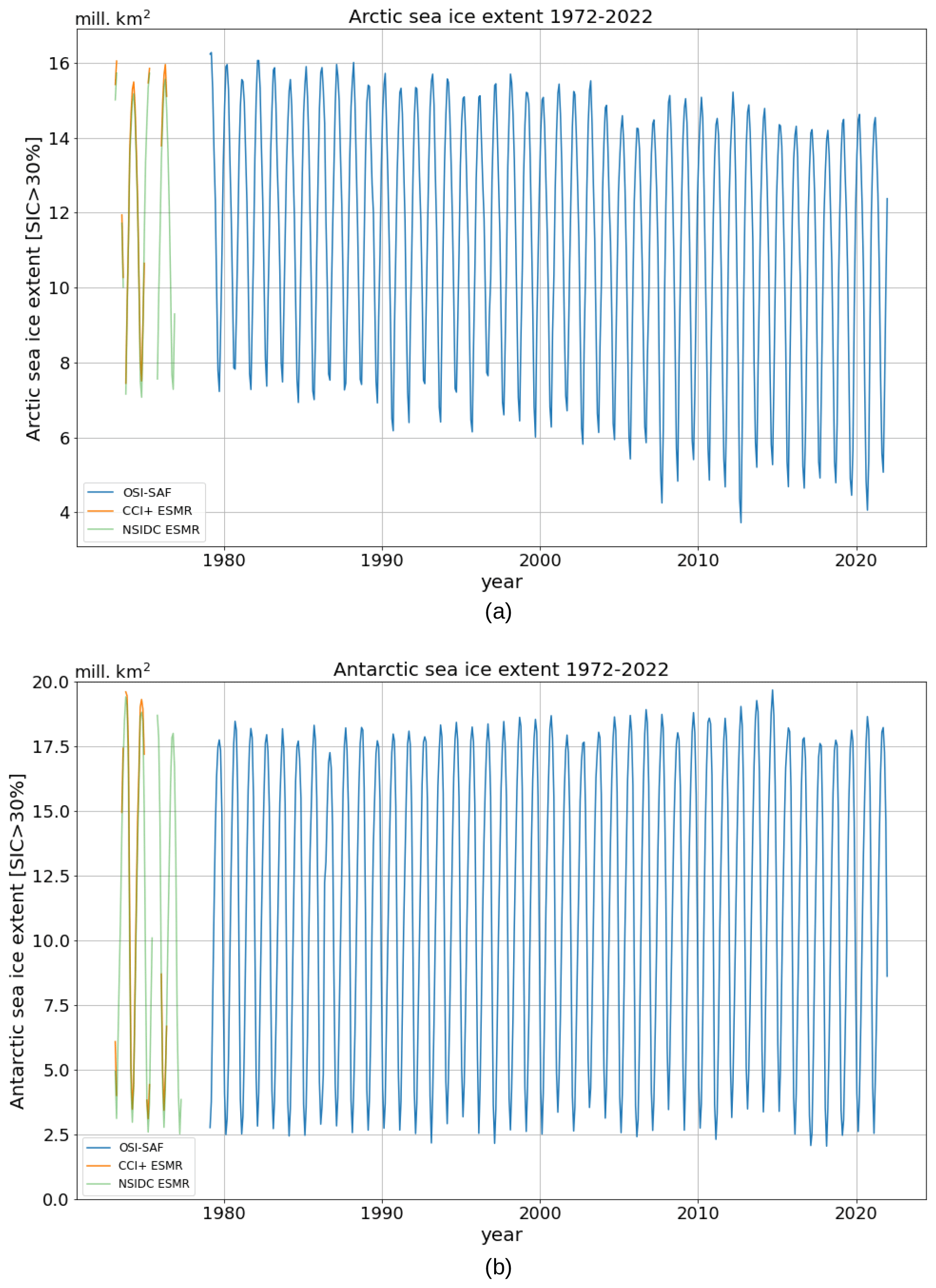
Figure 9Monthly sea ice extent time series for the (a) Arctic and (b) Antarctic based on the cice>30 % threshold. The orange curve shows values in the ESMR dataset which have 99 % coverage of the hemisphere monthly, while the blue curve is based on the SIC products from the OSI-SAF (EUMETSAT, 2017a, b), where the cice>30 % threshold was applied as in EUMETSAT (2017c). The green line represents the NSIDC's ESMR SIC product (Parkinson et al., 2004).
Comparisons between different sea ice products and the new ESMR dataset proved to be more difficult than initially expected, since not only the processing algorithms but also the land masks, map projections, and dataset grids differ. We were not able to find two independent SIC datasets for 1978 onwards and 1972–1977 which share exactly the same land mask.
Thus, it was decided at the beginning of the processing to use the same land mask as the OSI-420 product (1978 onwards) (EUMETSAT, 2020) for our ESMR dataset, i.e., a 25 km equal-area grid (EASE-2 version 2) land mask, to at least ensure a fair comparison between these two datasets. The NSIDC ESMR dataset (green line in Fig. 9) used a different land mask with a polar stereographic projection (Parkinson et al., 2004), but it was still compared to our ESMR dataset.
The difference in SIE is therefore also influenced by the different projections of the data; however, the area difference between the projections is relatively small (only a few thousand km2), so even a re-projection is expected to yield minimal differences compared to the differences caused by the use of different land masks. The comparison of different land masks is complicated by the varying sea ice extent, which exposes more or less land throughout its annual cycle and thus changes the number of grid points affected by the land mask.
The land mask land area differs between the OSI-SAF and NSIDC ESMR land masks. A comparison of land and ocean points between the NSIDC land mask and the OSI-SAF land mask showed a difference for the Northern Hemisphere of 460 000 km2 (north of 60° N), where the NSIDC land mask has more land, while the difference is the opposite and much smaller in the Southern Hemisphere – only 79 000 km2 (south of 60° S) – with the OSI-SAF's land mask having slightly more land. More land points in the land mask result in fewer available grid points for potential sea ice. The difference in Southern Hemisphere sea ice extent is significantly larger and opposite to the expected contrast from the land mask difference. In the Northern Hemisphere, it is not very clear how much of the SIE difference can be accounted for by the land mask or by algorithm differences. However, since the SIE differences vary a lot, and the differences in the Southern Hemisphere clearly cannot be explained by the land mask difference alone, it is likely that most of the SIE differences come from the algorithms and processing methods, such as the atmospheric correction and tie point calculation.
The blue curve in Fig. 9 is based on OSI-SAF's SIC products OSI-450 and OSI-430-b (EUMETSAT, 2017b, a). The shown extend corresponds to the SIE of the OSI-420 product (EUMETSAT, 2020) but with a 30 % instead of a 15 % sea ice threshold applied, matching the OSI-402-d sea ice extent product (EUMETSAT, 2017c).
Compared to the more common 15 %, the 30 % threshold was better suited to a comparison between different ESMR SIE datasets due to the relatively high noise level, which can be seen from the total uncertainty in Fig. 5. The uncertainty algorithm has been applied for easier data assessment and comparison to other datasets.
A large number of ESMR data are currently filtered out, and the 99 % threshold for inclusion in the monthly timeline in particular filters out the second half of the ESMR data, where large data gaps occurred, as seen in Fig. 8.
The filters worked as expected and removed erroneous TB values from the raw data. A reprocessing of the data to rescue more of the currently filtered out data points from the 20 % of ESMR data files is planned. Two approaches will be used to improve the data selection during the next processing. One approach consists of making changes to the set of filters, i.e., performing an adjustment of the filter thresholds, testing different filters, and the possible incorporation of an incidence angle dependency into the data selection. The other approach is to recalibrate some of the erroneous data files that have shown some systematic offsets to rescue whole swaths.
To reduce the uncertainty caused by atmospheric noise, the brightness temperatures were corrected with an RTM that used several atmospheric parameters from NWP (ERA5) data, such as water vapor and wind, as input. This correction showed a consistent reduction of the standard deviation of the brightness temperatures for water points in both hemispheres, as can be seen from Fig. 5. The correction was less steady over ice surfaces, since the RTM did not describe all relevant processes related to the snow and ice, which are the main noise source over sea ice. Such processes include sea ice deformation, the creation of leads or ridges, and changes in the snow layer, e.g., changes in snow depth, snow density, and grain size but also melting and refreezing, which influences scattering and emission processes inside the layer. Atmospheric noise caused by, e.g., water vapor and cloud liquid water influences the TB over sea ice, but its influence is smaller: only around one-third of the total noise (Tonboe et al., 2021). By correcting for atmospheric effects with ERA5 data, we might have introduced some noise into the angular dependency of the SIC due to the use of an incident-angle-dependent emissivity in the RTM (Fig. 1 and Table 1).
To avoid biases from the RTM and the NWP data, dynamical tie points have been used, which also calibrate the algorithm for seasonal variations and instrument drift. However, we currently use mean tie points that are independent of the incident angle. Therefore, a possible improvement to a future version of the dataset might be accomplished by using angle-dependent tie points instead.
Even after filtering the data for obvious errors, it is clear that there are still issues with the absolute calibration of the instrument (Comiso and Zwally, 1980). For example, after the hot-load anomaly in 1973, the ocean TB in the Southern Hemisphere is several kelvin below the TB level before the anomaly, and in 1976 there is a dip in May and June followed by a sharp increase in TB (Zwally et al., 1983). Low-frequency (with timescales ≥ days) TB variations and regional variations at hemispherical scales are compensated for by the dynamical SIC algorithm tie points (Tonboe et al., 2016).
In spite of data gaps and calibration issues, the experimental NIMBUS satellite program was very successful. Applying modern processing methodologies, including dynamical tie points and atmospheric noise reduction of the TB values, reduces the noise over both ice and open water consistently. This newly processed ESMR sea ice dataset extends the existing sea ice climate data record (CDR) with an important period from the 1970s. This extension of the SIE record contributes to the United Nations Sustainable Development Goals (SDGs) related to climate change by providing more observations for longer-term assessments of Arctic and Antarctic sea ice changes.
The newly processed ESMR data have been released through the ESA CCI Open Data Portal: https://climate.esa.int/en/odp/#/project/sea-ice (last access: 8 March 2024) and at DOI: https://doi.org/10.5285/34a15b96f1134d9e95b9e486d74e49cf (Tonboe et al., 2023).
In this paper, we have presented a new SIC dataset covering the period 1972–1977, obtained using the ESMR data from the NIMBUS 5 satellite. The dataset consists of resampled daily NetCDF files for the Northern and Southern hemispheres. The SIC, associated uncertainties, and processing flags are included in the dataset. The uncertainties follow the same principles as those of the EUMETSAT SIC CDR, including both algorithm and resampling uncertainties. The choice to use the same land mask, spatial grid, and projection as for EUMETSAT's SIC CDR make comparisons between the time periods easier.
A comparison to NSIDC's ESMR SIC product and the OSI-SAF CDR showed that the seasonal pattern is very similar to NSIDC's ESMR SIC product, but our product shows systematically larger SIE values which can not be explained by differences between land masks alone. For the Northern Hemisphere, our SIE values match the levels in the 1980s from the OSI-SAF CDR with the same land mask, while values in the Southern Hemisphere in the 1970s are larger than those in the 1980s.
Compatibility with the EUMETSAT's SIC CDR was achieved by using a similar processing chain. The processing included atmospheric noise reduction with the use of an RTM and the ERA5 atmospheric data, which lowered the standard deviation of the TBs consistently. Additionally, dynamical tie points were used to avoid biases from the RTM and NWP data as well as to adjust for seasonal variability and instrument biases. To ensure better data assessment in analysis and models and easier comparison to other datasets, temporally and regionally varying uncertainty estimates have been included in our ESMR dataset.
Table A1The data variables in the NetCDF processing input file and a description of each variable.
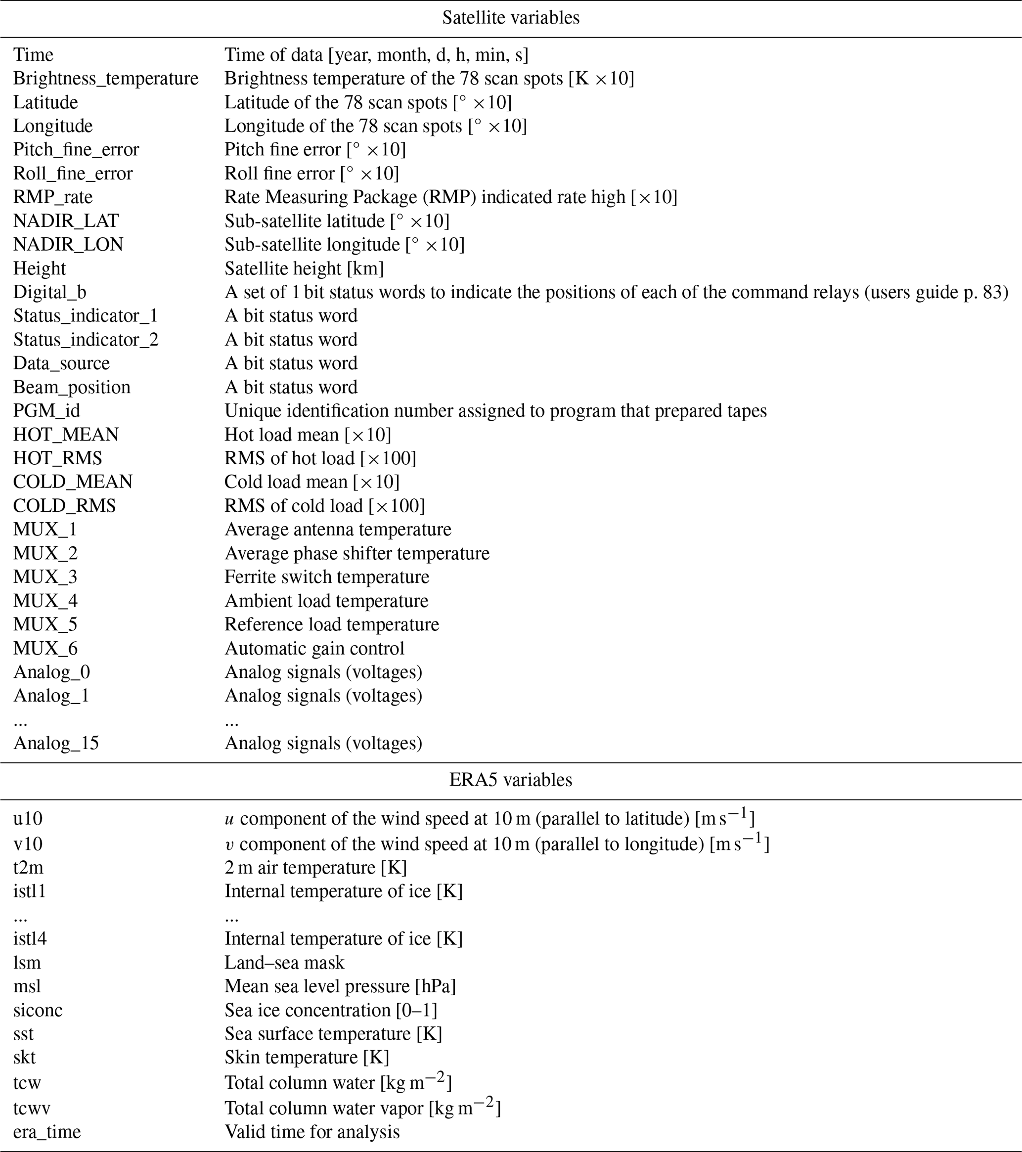
Table A2The output variables stored in the daily NetCDF files and a description of each variable.
WK performed the experiments, investigated the data, developed software, and wrote the manuscript, with contributions from all authors. RT contributed to the conceptualization, methodology, software, investigation, original draft, review, and editing of the manuscript and provided supervision throughout the work. JS contributed with critical feedback that shaped the interpretation and presentation of the data and improved the manuscript through reviewing and editing.
The contact author has declared that none of the authors has any competing interests.
Publisher’s note: Copernicus Publications remains neutral with regard to jurisdictional claims made in the text, published maps, institutional affiliations, or any other geographical representation in this paper. While Copernicus Publications makes every effort to include appropriate place names, the final responsibility lies with the authors.
This work is part of the ESA Climate Change Initiative (ESA CCI) program's Sea Ice CCI (Sea_Ice_cci) project and the Danish National Centre for Climate Research (NCKF) at the Danish Meteorological Institute (DMI). The authors would like to thank Tadea Veng, Roberto Saldo, Thomas Lavergne, Atle Sørensen, and Leif Toudal Pedersen for their inputs and valuable feedback. We would also like to thank Imke Sievers, John Andrew Dawson, and Andreas Svejgaard Jensen for developing and testing the data filters described in Sect. 2.
This paper was edited by Alexander Fraser and reviewed by two anonymous referees.
Andersen, S., Tonboe, R., Kern, S., and Schyberg, H.: Improved retrieval of sea ice total concentration from spaceborne passive microwave observations using Numerical Weather Prediction model fields: An intercomparison of nine algorithms, Remote Sens. Environ., 104, 374–392, https://doi.org/10.1016/j.rse.2006.05.013, 2006. a, b, c
Bell, B., Hersbach, H., Berrisford, P., Dahlgren, P., Horányi, A., Muñoz Sabater, J., Nicolas, J., Radu, R., Schepers, D., Simmons, A., Soci, C., and Thépaut, J-N.: ERA5 hourly data on single levels from 1950 to 1978 (preliminary version), Copernicus Climate Change Service (C3S) Climate Data Store (CDS) [data set], https://cds.climate.copernicus.eu/cdsapp#!/dataset/reanalysis-era5-single-levels-preliminary-back-extension?tab=overview (last access: 6 August 2021), 2020. a
Bell, B., Hersbach, H., Simmons, A., Berrisford, P., Dahlgren, P., Horányi, A., Muñoz-Sabater, J., Nicolas, J., Radu, R., Schepers, D., Soci, C., Villaume, S., Bidlot, J.-R., Haimberger, L., Woollen, J., Buontempo, C., and Thépaut, J.-N.: The ERA5 global reanalysis: Preliminary extension to 1950, Q. J. Roy. Meteor. Soc., 147, 4186–4227, https://doi.org/10.1002/qj.4174, 2021. a
Chapman, W. L. and Walsh, J. E.: Long-range prediction of regional sea ice anomalies in the Arctic, Weather Forecast., 6, 271–288, https://doi.org/10.1175/1520-0434(1991)006<0271:LRPORS>2.0.CO;2, 1991. a
Cheon, W. G. and Gordon, A. L.: Open-ocean polynyas and deep convection in the Southern Ocean, Sci. Rep., 9, 6935, https://doi.org/10.1038/s41598-019-43466-2, 2019. a
Comiso, J. C. and Zwally, H. J.: Correction for anomalous time dependent shifts in the brightness temperature from Nimbus 5 ESMR, NASA TM-82055, Greenbelt, Maryland, 18 pp., https://ntrs.nasa.gov/citations/19810006910 (last access: 8 March 2024), 1980. a, b
Comiso, J. C., Cavalieri, D. J., Parksinson, C. L., and Gloersen, P.: Passive microwave algorithms for sea ice concentration: A comparison of two techniques, Remote Sens. Environ., 60, 357–384, 1997. a
Comiso, J. C., Wadhams, P., Pedersen, L. T., and Gersten, R. A.: Seasonal and interannual variability of the Odden ice tongue and a study of environmental effects, J. Geophys. Res., 106, 9093–9116, https://doi.org/10.1029/2000JC000204, 2001. a, b
ESA Climate Office, CCI+: Sea Ice ECV ESMR Sea Ice Concentration Product User Guide for ESMR (PUG-ESMR), Reference: D4.2-ESMR, Issue 1.1, https://climate.esa.int/en/projects/sea-ice/Sea-Ice-Key-Documents/ (last access: 20 December 2023), 2022. a
EUMETSAT: Ocean and Sea Ice Satellite Application Facility Global sea ice concentration interim climate data record 2016-onwards (v2.0, 2017), OSI-430-b, EUMETSAT Data Center [2016–2022] [data set], https://doi.org/10.15770/EUM_SAF_OSI_NRT_2008 (last access: 19 October 2022), 2017a. a, b, c
EUMETSAT: Ocean and Sea Ice Satellite Application Facility, Global sea ice concentration climate data record 1979–2015 (v2.0, 2017), OSI-450, EUMETSAT Data Center [1979–2015] [data set], https://doi.org/10.15770/EUM_SAF_OSI_0008, 2017b. a, b, c
EUMETSAT: Ocean and Sea Ice Satellite Application Facility, Global Sea Ice Edge product, OSI-402-d, EUMETSAT Data Center [data set], https://www.osi-saf.eumetsat.int (last access: 19 October 2022), 2017c. a, b
EUMETSAT: Ocean and Sea Ice Satellite Application Facility, Sea ice index 1979–onwards (v2.1, 2020), OSI-420, OSI SAF FTP server: 1979–2019, Northen & Southern Hemisphere, OSI SAF Sea Ice Index v2.1, EUMETSAT Data Center [data set], https://osisaf-hl.met.no/v2p1-sea-ice-index (last access: 19 October 2022), 2020. a, b
Ferreira, D., Marshall, J., Bitz, C. M., Solomon, S., and Plumb, A.: Antarctic Ocean and Sea Ice Response to Ozone Depletion: A Two-Time-Scale Problem, J. Climate, 28, 1206–1226, https://doi.org/10.1175/JCLI-D-14-00313.1, 2015. a
Fogt, R. L., Sleinkofer, A. M., Raphael, M. N., and Handcock, M. S.: A regime shift in seasonal total Antarctic sea ice in the twentieth century, Nat. Clim. Change 12, 54–62, https://doi.org/10.1038/s41558-021-01254-9, 2022. a
Hersbach, H., Bell, B., Berrisford, P., Hirahara, S., Horányi, A., Muñoz-Sabater, J., Nicolas, J., Peubey, C., Radu, R., Schepers, D., Simmons, A., Soci, C., Abdalla, S., Abellan, X., Balsamo, G., Bechtold, P., Biavati, G., Bidlot, J., Bonavita, M., and Thépaut, J.-N.: The ERA5 global reanalysis, Q. J. Roy. Meteor. Soc., 146, 1999–2049, https://doi.org/10.1002/qj.3803, 2020. a, b
Jena, B., Ravichandran, M., and Turner, J.: Recent reoccurrence of large open-ocean polynya on the Maud Rise seamount, Geophys. Res. Lett., 46, 4320–4329, https://doi.org/10.1029/2018GL081482, 2019. a, b
Knight, R. W.: Introduction to a New Sea-Ice Database, Ann. Glaciol., 5, 81–84, https://doi.org/10.3189/1984AoG5-1-81-84, 1984. a
Kongoli, C., Boukabara, S.-A., Yan, B., Weng, F., and Ferraro, R.: A New Sea-Ice Concentration Algorithm Based on Microwave Surface Emissivities–Application to AMSU Measurements, IEEE T. Geosci. Remote, 49, 175–189, https://doi.org/10.1109/TGRS.2010.2052812, 2011. a
Lavergne, T., Sørensen, A. M., Kern, S., Tonboe, R., Notz, D., Aaboe, S., Bell, L., Dybkjær, G., Eastwood, S., Gabarro, C., Heygster, G., Killie, M. A., Brandt Kreiner, M., Lavelle, J., Saldo, R., Sandven, S., and Pedersen, L. T.: Version 2 of the EUMETSAT OSI SAF and ESA CCI sea-ice concentration climate data records, The Cryosphere, 13, 49–78, https://doi.org/10.5194/tc-13-49-2019, 2019. a, b, c, d
Markus, T. and Cavalieri, D. J.: The AMSR-E NT2 sea ice concentration algorithms: its basis and implementation, Journal of the Remote Sensing Society of Japan, 29, 216–225, 2009. a
Meissner, T. and Wentz, F.: AMSR Ocean Algorithm, Algorithm Theoretical Basis Document (ATBD) Version 2, https://eospso.gsfc.nasa.gov/sites/default/files/atbd/atbd-amsr-ocean.pdf (last access: 8 March 2024), 2000. a, b
Meissner, T. and Wentz, F.: The emissivity of the ocean surface between6 and 90 ghz over a large range of windspeeds and earth incidence angles, IEEE T. Geosci. Remote, 50, 3004–3026, 2012. a
NASA: The NIMBUS 5 data catalog, data orbits 8843 – 9660, volume 12, final report, 1 October–30 November 1974, NASA CR 157882, https://ntrs.nasa.gov/citations/19790074718 (last access: 8 March 2024), 1974. a, b
NASA Goddard Space Flight Center (GSFC): ESMR/Nimbus-5 Level 1 Calibrated Brightness Temperature V001, Greenbelt, MD, USA, Goddard Earth Sciences Data and Information Services Center (GES DISC), https://disc.gsfc.nasa.gov/datacollection/ESMRN5L1_001.html (last access: 26 June 2019), 2016. a, b, c, d
Onarheim, I., Eldevik, T., Smedsrud, L., and Stroeve, J.C.: Seasonal and Regional Manifestation of Arctic Sea Ice Loss, J. Climate, 31, 4917–4932, https://doi.org/10.1175/JCLI-D-17-0427.1, 2018. a
Parkinson, C. L., Comiso, J. C., Zwally, H. J., Cavalieri, D. J., Gloersen, P., and Campbell, W. J.: Arctic sea ice, 1973-1976: satellite passive-microwave observations, NASA special publications, NASA SP-489, https://ntrs.nasa.gov/citations/19870015437 (last access: 8 March 2024), 1987. a, b
Parkinson, C. L., Comiso, J. C., and Zwally, H. J.: Nimbus-5 ESMR Polar Gridded Brightness Temperatures, Version 2 (User Guide), Boulder, Colorado USA, NASA National Snow and Ice Data Center Distributed Active Archive Center [data set], https://doi.org/10.5067/CIRAYZROIYF9, 1999. a
Parkinson, C. L., Comiso, J. C., and Zwally, H. J.: Nimbus-5 ESMR Polar Gridded Sea Ice Concentrations, Version 1, edited by: Meier, W. and Stroeve, J., Boulder, Colorado USA, NASA National Snow and Ice Data Center Distributed Active Archive Center [data set], https://doi.org/10.5067/W2PKTWMTY0TP, 2004. a, b, c, d, e, f
Rayner, N. A., Parker, D. E., Horton, E. B., Folland, C. K., Alexander, L. V., Rowell, D. P., Kent, E. C., and Kaplan, A.: Global analyses of sea surface temperature, sea ice, and night marine air temperature since the late nineteenth century, J. Geophys. Res., 108, 4407, https://doi.org/10.1029/2002JD002670, 2003. a, b
Sabatini, R. R. (Ed.): The Nimbus 5 user's guide: NASA Goddard Space Flight Center, U.S. Govt. Printing Office, https://ntrs.nasa.gov/citations/19740020209 (last access: 8 March 2024), 1972. a
Schanda, E.: Physical Fundamentals of Remote Sensing, Springer-Verlag, Berlin Heidelberg, ISBN 978-3-540-16236-0, https://doi.org/10.1007/978-3-642-48733-0, 1986. a
Schroeter, S., O'Kane, T. J., and Sandery, P. A.: Antarctic sea ice regime shift associated with decreasing zonal symmetry in the Southern Annular Mode, The Cryosphere, 17, 701–717, https://doi.org/10.5194/tc-17-701-2023, 2023. a
Singh, H. A., Polvani, L. M., and Rasch, P. J.: Antarctic sea ice expansion, driven by internal variability, in the presence of increasing atmospheric CO2, Geophys. Res. Lett., 46, 14762–14771, https://doi.org/10.1029/2019GL083758, 2019. a
Stammerjohn, S. E., Martinson, D. G., Smith, R. C., Yuan, X., and Rind, D.: Trends in Antarctic annual sea ice retreat and advance and their relation to El Niño–Southern Oscillation and Southern Annular Mode variability, J. Geophys. Res., 113, C03S90, https://doi.org/10.1029/2007JC004269, 2008. a
Stroeve, J. C. and Notz, D.: Changing state of Arctic sea ice across all seasons, Environ. Res. Lett., 13, 103001, https://doi.org/10.1088/1748-9326/aade56, 2018. a
Sun, S. and Eisenman, I.: Observed Antarctic sea ice expansion reproduced in a climate model after correcting biases in sea ice drift velocity, Nat. Commun., 12, 1060, https://doi.org/10.1038/s41467-021-21412-z, 2021. a
Svendsen, E., Kloster, K., Farrelly, B., Johannessen, O. M., Johannessen, J. A., Campbell, W. J., Gloersen, P., Cavalieri, D., and Mätzler, C.: Norwegian Remote Sensing Experiment: Evaluation of the Nimbus 7 scanning multichannel microwave radiometer for sea ice research, J. Geophys. Res., 88, 2781–2791, https://doi.org/10.1029/JC088iC05p02781, 1983. a
Thompson, D. W. J. and Solomon, S.: Interpretation of Recent Southern Hemisphere Climate Change, Science, 296, 5569, 895–899, https://doi.org/10.1126/science.1069270, 2002. a
Titchner, H. A. and Rayner, N. A.: The Met Office Hadley Centre sea ice and sea surface temperature data set, version 2: 1. Sea ice concentrations, J. Geophys. Res.-Atmos., 119, 2864–2889, https://doi.org/10.1002/2013JD020316, 2014. a
Tonboe, R. T.: The simulated sea ice thermal microwave emission at window and sounding frequencies, Tellus A, 62, 333–344, 2010. a
Tonboe, R. T., Eastwood, S., Lavergne, T., Sørensen, A. M., Rathmann, N., Dybkjær, G., Pedersen, L. T., Høyer, J. L., and Kern, S.: The EUMETSAT sea ice concentration climate data record, The Cryosphere, 10, 2275–2290, https://doi.org/10.5194/tc-10-2275-2016, 2016. a, b, c, d
Tonboe, R., Nandan, V., Mäkynen, M., Pedersen, L., Kern, S., Lavergne, T., Øelund, J., Dybkjær, G., Saldo, R., and Huntemann, M.: Simulated Geophysical Noise in Sea Ice Concentration Estimates of Open Water and Snow-Covered Sea Ice, IEEE J. Sel. Top. Appl., 15, 1309–1326, https://doi.org/10.1109/JSTARS.2021.3134021, 2021. a, b
Tonboe, R. T., Kolbe, W. M., Toudal Pedersen, L., Lavergne, T., Sørensen, A., and Saldo, R.: ESA Sea Ice Climate Change Initiative (Sea_Ice_cci): Nimbus-5 ESMR Sea Ice Concentration, version 1.0., NERC EDS Centre for Environmental Data Analysis [data set], https://doi.org/10.5285/34a15b96f1134d9e95b9e486d74e49cf, 2023. a, b
Turner, J., Comiso, J. C., Marshall, G. J., Lachlan-Cope, T. A., Bracegirdle, T., Maksym, T., Meredith, M. P., Wang, Z., and Orr, A.: Non-annular atmospheric circulation change induced by stratospheric ozone depletion and its role in the recent increase of Antarctic sea ice extent, Geophys. Res. Lett., 36, L08502, https://doi.org/10.1029/2009GL037524, 2009. a
Ulaby, F. T., Moore, M. K., and Fung, A. K.: Microwave Remote Sensing, Active and Passive, Vol. 3, Artech House, Norwood, MA, ISBN 0890061920, 9780890061923, 1986. a
Veng, T.: Mapping of sea ice using NIMBUS 5 ESMR satellite data, Master thesis, DTU Space, https://findit.dtu.dk/en/catalog/6059da9cd9001d016554ff7a (last access: 8 March 2024), 2021. a
Walsh, J. E.: A data set on Northern Hemisphere sea ice extent, 1953–76, World Data Center-A for Glaciology, Boulder, Colorado, Glaciological Data Report GD-2, 49–51, https://nsidc.org/sites/default/files/documents/other/gd-2_web.pdf (last access: 8 March 2024), 1978. a
Walsh, J. E. and Johnson, C. M.: An analysis of Arctic sea ice fluctuations, 1953-−1977, J. Phys. Oceanogr., 9, 580-−591, https://doi.org/10.1175/1520-0485(1979)009<0580:AAOASI>2.0.CO;2, 1979. a
Walsh, J. E. and Chapman, W. L.: 20th-century sea-ice variations from observational data, Ann. Glaciol., 33, 444–448, https://doi.org/10.3189/172756401781818671, 2001. a
Walsh, J. E., Fetterer, F., Stewart, J. S., and Chapman, W. L.: A database for depicting Arctic sea ice variations back to 1850, Geogr. Rev., 107, 89–107, https://doi.org/10.1111/j.1931-0846.2016.12195.x, 2017. a
Walsh, J. E., Chapman, W. L., Fetterer, F., and Stewart, J. S.: Gridded Monthly Sea Ice Extent and Concentration, 1850 Onward, Version 2, Boulder, Colorado USA, National Snow and Ice Data Center [data set], https://doi.org/10.7265/jj4s-tq79, 2019. a
Wang, G., Hendon, H. H., Arblaster, J. M., Lim, E.-P., Abhik, S., and Rensch, P. V.: Compounding tropical and stratospheric forcing of the record low Antarctic sea-ice in 2016, Nat. Commun., 10, 13, https://doi.org/10.1038/s41467-018-07689-7, 2019. a
Wentz, F. J.: A model function for ocean microwave brightness temperatures, J. Geophys. Res., 88, 1892–1908, https://doi.org/10.1029/JC088iC03p01892, 1983. a, b
Wentz, F. J.: A well-calibrated ocean algorithm for special sensor microwave/imager, J. Geophys. Res., 102, 8703–8718, https://doi.org/10.1029/96JC01751, 1997. a, b, c, d
Zwally, H. J., Comiso, J. C., Parkinson, C. L., Campbell,W. J., Carsey, F. D., and Gloersen, P.: Antarctic sea ice 1973–1976: Satellite passive microwave observations, NASA SP-459, Washington DC, pp. 206, https://ntrs.nasa.gov/citations/19840002650 (last access: 8 March 2024), 1983. a