the Creative Commons Attribution 4.0 License.
the Creative Commons Attribution 4.0 License.
 | 10 Jan 2024
CMEMS-LSCE: a global, 0.25°, monthly reconstruction of the surface ocean carbonate system
Thi-Tuyet-Trang Chau
Marion Gehlen
Nicolas Metzl
Frédéric Chevallier
Observation-based data reconstructions of global surface ocean carbonate system variables play an essential role in monitoring the recent status of ocean carbon uptake and ocean acidification, as well as their impacts on marine organisms and ecosystems. So far, ongoing efforts are directed towards exploring new approaches to describe the complete marine carbonate system and to better recover its fine-scale features. In this respect, our research activities within the Copernicus Marine Environment Monitoring Service (CMEMS) aim to develop a sustainable production chain of observation-derived global ocean carbonate system datasets at high space–time resolutions. As the start of the long-term objective, this study introduces a new global 0.25∘ monthly reconstruction, namely CMEMS-LSCE (Laboratoire des Sciences du Climat et de l'Environnement) for the period 1985–2021. The CMEMS-LSCE reconstruction derives datasets of six carbonate system variables, including surface ocean partial pressure of CO2 (pCO2), total alkalinity (AT), total dissolved inorganic carbon (CT), surface ocean pH, and saturation states with respect to aragonite (Ωar) and calcite (Ωca). Reconstructing pCO2 relies on an ensemble of neural network models mapping gridded observation-based data provided by the Surface Ocean CO2 ATlas (SOCAT). Surface ocean AT is estimated with a multiple-linear-regression approach, and the remaining carbonate variables are resolved by CO2 system speciation given the reconstructed pCO2 and AT; 1σ uncertainty associated with these estimates is also provided. Here, σ stands for either the ensemble standard deviation of pCO2 estimates or the total uncertainty for each of the five other variables propagated through the processing chain with input data uncertainty. We demonstrate that the 0.25∘ resolution pCO2 product outperforms a coarser spatial resolution (1∘) thanks to higher data coverage nearshore and a better description of horizontal and temporal variations in pCO2 across diverse ocean basins, particularly in the coastal–open-ocean continuum. Product qualification with observation-based data confirms reliable reconstructions with root-mean-square deviation from observations of less than 8 %, 4 %, and 1 % relative to the global mean of pCO2, AT (CT), and pH. The global average 1σ uncertainty is below 5 % and 8 % for pCO2 and Ωar (Ωca), 2 % for AT and CT, and 0.4 % for pH relative to their global mean values. Both model–observation misfit and model uncertainty indicate that coastal data reproduction still needs further improvement, wherein high temporal and horizontal gradients of carbonate variables and representative uncertainty from data sampling would be taken into account as a priority. This study also presents a potential use case of the CMEMS-LSCE carbonate data product in tracking the recent state of ocean acidification. The data associated with this study are available at https://doi.org/10.14768/a2f0891b-763a-49e9-af1b-78ed78b16982 (Chau et al., 2023).
- Article
(15997 KB) - Full-text XML
- BibTeX
- EndNote


Between 1750 and 2019, the ocean took up an estimated 25 % (or 170 ± 20 Pg C) of total cumulated anthropogenic CO2 (685 ± 75 Pg C) emitted to the atmosphere (IPCC AR6 – the Sixth Assessment Report of the United Nations Intergovernmental Panel on Climate Change, Canadell et al., 2021). While the uptake of anthropogenic CO2 mitigates global warming, it also profoundly modifies seawater chemistry in a suite of well-understood reactions (Orr et al., 2005), leading to an increase in hydrogen ion concentration ([H+]), as well as a decrease in carbonate ion concentration ([]) and in the saturation state of seawater (Ω) with respect to calcium carbonate minerals (CaCO3). The increase in hydrogen ion concentration ([H+]) is commonly reported as a decrease in pH (pH = −log [H+]) and referred to as ocean acidification.
Changes in carbonate chemistry impact calcifying plankton and benthos as a direct result of decreasing seawater saturation state with respect to CaCO3 (Fabry et al., 2008; Thomsen et al., 2015). Ocean acidification also modifies the production of marine trace gases exchanged at the air–sea interface (Hopkins et al., 2020), the availability of nutrients fuelling primary production (Doney et al., 2009), and the speciation of pollutants (Millero et al., 2009; Hoffmann et al., 2012). These chemical changes interact with warming and ocean deoxygenation to drive major changes in marine ecosystems (Doney et al., 2020) and to alter global biogeochemical cycles with the potential for feeding back to radiative forcing (Gehlen et al., 2011; Hopkins et al., 2020). The likelihood of major disruptive impacts of ocean acidification on marine ecosystems, if future CO2 emissions were to go unabated, is reflected by the Sustainable Development Goal 14.3 (SDG 14.3) – namely to “Reduce Ocean Acidification: minimize and address impacts of ocean acidification” (https://www.globalgoals.org/14-life-below-water, last access: 20 March 2023). While not specifically mentioned, moving towards SDG 14.3 implies the understanding of historical and contemporary carbonate chemistry and its mean state, trends, and variability.
In situ time series have played an important role in monitoring ocean acidification over the last decades (Bates et al., 2014; Lauvset et al., 2015; Sutton et al., 2019; Pérez et al., 2021; Leseurre et al., 2022; Skjelvan et al., 2022). At these sites, seawater pH (Ω) has been either directly measured or calculated from measurements of other carbonate system variables. These variables include surface ocean partial pressure of CO2 (pCO2), total alkalinity (AT), and dissolved inorganic carbon (CT). While changes in the time series of carbonate system variables reflect well the impacts of enhanced anthropogenic CO2 uptake on ocean chemistry at a local scale (Steinberg et al., 2001; González-Dávila and Santana-Casiano, 2009; Dore et al., 2009; Bates et al., 2014; Pérez et al., 2021), the reliable upscaling to large ocean regions or entire basins requires a significant extension of the existing observing network (Lauvset et al., 2015; Bakker et al., 2016; Sutton et al., 2019; Lauvset et al., 2022a).
Time series data are completed by bottle data from international cruises. These data are synthesized by the Global Ocean Data Analysis Project v2.2022 (GLODAPv2.2022) and include about 1.4 million measurements of surface-to-interior ocean pH, AT, CT, and other parameters (Lauvset et al., 2022b, https://www.glodap.info/, last access: 30 September 2022). Likewise, underway measurements of near-surface CO2 fugacity, i.e. pCO2 corrected for non-ideal gas behaviour, have been compiled in the Surface Ocean CO2 ATlas (SOCAT) since its first release in 2011 (Pfeil et al., 2013). The latest version, SOCATv2022, yields approximately 33.7 million high-quality controlled data (Bakker et al., 2022, http://www.socat.info/, last access: 17 June 2022). Despite millions of observations being available, data coverage is still modest; e.g. CO2 fugacity samples over the global ocean cover less than 2 % of its surface for each month in the last 3 decades (Bakker et al., 2016; Hauck et al., 2020). Mapping methods have thus become an essential tool in ocean carbon cycle research, allowing us to interpolate or extrapolate these sparse measurements into space–time-varying fields of carbonate system variables.
Recent years have seen the rapid development of machine learning approaches to map global surface ocean pCO2 (see Rödenbeck et al., 2013; Landschützer et al., 2016; Denvil-Sommer et al., 2019; Gregor et al., 2019; Chau et al., 2022b, for instance). Thanks to these efforts, the carbon cycle community can now draw on an ensemble of reconstructions for the observation-based assessment of the ocean carbon sink (Friedlingstein et al., 2022). However, only a few global observation-based reconstructions are available for pH, AT, CT, and Ω with respect to calcite and aragonite (see Gregor and Gruber, 2021, for a review). The reconstruction of global distributions of these variables is hampered by an insufficient amount of direct measurements (Bakker et al., 2016; Lauvset et al., 2022a). Alternatively, the complete carbonate system can be obtained by speciation given the information of any coupling of pCO2, pH, AT or CT together with chemical (e.g. phosphate, silicate, nitrate) and physical variables (e.g. temperature, salinity), as well as corresponding dissociation constants (Park, 1969; Lewis and Wallace, 1998; Dickson et al., 2007).
Regardless of the developments in different observation-based estimation methods, Takahashi et al. (2014), Iida et al. (2021), and Gregor and Gruber (2021) propose global climatologies or monthly varying fields of all variables of the carbonate system, i.e. pCO2, pH, AT, CT, and Ω. These data products have a spatial resolution of 1∘ (∼ 100 km × 100 km) or even coarser. Nevertheless, the variations in carbonate system variables over the coastal regions where their instantaneous gradients are driven by smaller-scale features like ocean upwelling, wind turbulence, eddies, water runoff, and sharp biological productivity (Jones et al., 2012; Bakker et al., 2016; Laruelle et al., 2017) are poorly described at such spatial resolutions. Here, we improve on existing studies by providing a global, 0.25∘, monthly observation-based product consisting of datasets of six core surface ocean carbonate system variables of the marine carbonate system and their associated 1σ uncertainty. This high-resolution data product covers the years from 1985 to 2021. Laboratoire des Sciences du Climat et de l'Environnement (LSCE) is in charge of the product within the European Copernicus Marine Environment Monitoring Service (CMEMS). Our product is referred to as CMEMS-LSCE hereafter.
The reconstruction of surface ocean carbonate system variables starts with the reconstruction of surface ocean pCO2 and AT in each regular grid of 1 month × 0.25∘ × 0.25∘ in the period 1985–2021 (444 months in total). Next, the variables of pH (reported on total scale), CT, and Ω are derived by speciation. The advantages of the combination of pCO2 and AT over others for the speciation of the carbonate system are as follows: (1) pCO2 is the most extensively measured parameter; (2) AT can be accurately predicted from salinity, temperature, and nutrient concentrations; and (3) the combination of these two prior variables results in the slightest uncertainty in pH estimates (Zeebe and Wolf-Gladrow, 2001; Lauvset and Gruber, 2014; Takahashi et al., 2014; Orr et al., 2018). The three main successive modules used in the CMEMS-LSCE production chain are summarized as follows:
- i.
Reconstruction of pCO2 (Sect. 3.1). The CMEMS-LSCE-FFNN ensemble-based approach (Chau et al., 2022b) is modified to map gridded datasets of SOCATv2022 CO2 fugacity and predictors in order to reconstruct pCO2 at a finer-spatial-scale resolution of 0.25∘ for every month in the period 1985–2021 (444 months in total). The spatial resolution of new feed-forward neural networks (FFNNs) is 16-fold higher than the original. By design, the ensemble of model outputs allows us to yield the best model estimate (i.e. ensemble mean) and model uncertainty (i.e. ensemble standard deviation) at each 0.25∘ grid cell and for each month. Global monthly reconstructions of pCO2 proposed by this study complement the previous climatological product by Landschützer et al. (2020), i.e. a combination of the two existing datasets covering, respectively the open ocean at 1∘ (Landschützer et al., 2016) and the coastal sector at 0.25∘ (Laruelle et al., 2017).
- ii.
Reconstruction of AT (Sect. 3.2). Locally interpolated alkalinity regression (LIAR; Carter et al., 2016, 2018) is chosen to estimate monthly total alkalinity over the global surface ocean. Various reconstruction methods for AT exist (see Carter et al., 2016; Broullón et al., 2019; Gregor and Gruber, 2021, for a review), but we choose LIAR due to its global applicability, simplicity in setting, and accuracy compared to other published approaches (Carter et al., 2018; Gregor and Gruber, 2021). Importantly, LIAR allows us to determine reconstruction uncertainty propagated from multiple sources of input uncertainties at desired model resolutions.
- iii.
Reconstruction of pH, CT, and saturation states with respect to aragonite (Ωar) and calcite (Ωca) (Sect. 3.3). CO2SYS (Lewis and Wallace, 1998; Van Heuven et al., 2011) is a standard software used for the speciation of carbonate parameters in the marine CO2 system (see Olsen et al., 2016; Bresnahan et al., 2021; Gregor and Gruber, 2021; Woosley, 2021, for a few of said parameters). A complement to the CO2SYS software (CO2SYS.v2) developed by Orr et al. (2018) is used to quantify the uncertainty associated with these carbonate system variables. All the input data uncertainties are propagated through the CO2SYS.v2 processing chain.
The global, monthly, 0.25∘ resolution datasets of surface carbonate variables are intensively evaluated against different observation-based products independent from our model fitting at a global scale to in situ locations. In Sect. 4, multiple metrics are proposed for product analyses and assessments. Results are presented in Sect. 5 with an emphasis on the evaluation of the best reconstruction and associated model uncertainty for each variable (Sect. 5). This section also highlights the advantages obtained with an increase in spatial resolution and presents an application of the CMEMS-LSCE product in tracking ocean acidification over the last 3 decades. Section 7 summarizes key results, discusses the potential for future model upgrades, and introduces possible product use cases. The high-resolution data product described in this paper (netCDF format) can be accessed via repository under the following data DOI: https://doi.org/10.14768/a2f0891b-763a-49e9-af1b-78ed78b16982 (Chau et al., 2023).
Bakker et al. (2022)Good (2022); Good and Worsfold (2022)Nardelli et al. (2016); Droghei et al. (2018)Menemenlis et al. (2008)Maritorena et al. (2010)Chevallier et al. (2005, 2010); Chevallier (2013)Takahashi et al. (2009)Garcia et al. (2019)Table 1Input data used in the reconstructions of CMEMS-LSCE carbonate system variables over the global ocean in 1985–2021.
Note: Last access was on 15 April 2022 for all input databases, except for SOCATv2022 data (17 June 2022) and WOA18 data (30 July 2022). Data products 1–8 are used in the pCO2 reconstruction. Products 2–3 and 9–11 are used to compute AT, CT, pH, Ωar, and Ωca. Global values of product uncertainty (data† or analysis errors expressed as σ) have been reported for (< 5 µatm), SST (0.15 ∘C), SSS (0.2 PSU), SSH (0.02 m), MLD (–), Chl a (0.03 mg m−3), xCO2 (–), (10 µatm), NO3 (1.8 µmol kg−1), SiO2 (3.6 µmol kg−1), and PO4 (0.12 µmol kg−1).
2.1 Input data products for surface ocean carbonate system reconstructions
Many observation-based products are used as predictors of our target carbonate system variables (Table 1). Global ocean maps of sea surface temperature (SST), sea surface salinity (SSS), sea surface height above geoid (SSH), and chlorophyll a (Chl a) come from the Copernicus Marine Environment Monitoring Service (CMEMS; Good et al., 2020; Nardelli et al., 2016; Droghei et al., 2018; Maritorena et al., 2010). Mixed-layer depth (MLD) fields belong to Estimating the Circulation and Climate of the Ocean project Phase II (ECCO2; Menemenlis et al., 2008). CO2 mole fractions (xCO2) are derived from the CO2 atmospheric inversion of the Copernicus Atmosphere Monitoring Service (CAMS; Chevallier et al., 2005, 2010; Chevallier, 2013). Surface ocean concentrations of nitrate (NO3), silicate (SiO2), and phosphate (PO4) are extracted from the World Ocean Atlas 2018 (WOA18; Garcia et al., 2019). The climatological pCO2 () product is provided by Lamont Doherty Earth Observatory (LDEO; Takahashi et al., 2009). Details of these products, including resource access, data coverage, and resolutions, are presented in Table 1.
With the exception of xCO2, nutrient concentrations, and , these input data products have original resolutions equivalent to or even finer than a spatial resolution of 0.25∘ and a temporal resolution of monthly. When mismatches in data resolutions appear, input data products are interpolated to fit the pre-defined model resolutions. The monthly average is applied for daily (hourly) data products, and the Climate Data Operators (CDO) remap operator is used to regrid the input data fields with spatial resolutions different from 0.25∘. The datasets of SST and xCO2 – the two key variables driving global pCO2 changes (Bates et al., 2014; Gruber et al., 2019; Landschützer et al., 2019; Chau et al., 2022b; Friedlingstein et al., 2022) – cover the full learning period and the whole globe, as expected. The other predictor data are not available before the 1990s, when new types of satellite measurements started, and one of them (i.e. Chl a) does not cover the high latitudes of the winter hemisphere. We therefore gap-fill the time series in an ad hoc manner, as in previous studies (Landschützer et al., 2016; Gregor et al., 2019; Chau et al., 2022b). Monthly climatologies of SSS, Chl a, and MLD computed based on the available data are used for each missing year. Likewise, climatologies plus linear trends of SSH following global warming effects serve for the pre-1993 period. Missing Chl a data in the high latitudes of the winter hemisphere are replaced by the minimum concentration of Chl a over the available data for the same grid cell (∼ 0.01 mg m−3). WOA18 nutrients and LDEO are already climatologies per se, and we apply them for all the analysis years (1985–2021). The sine function is applied to convert latitude, while both the sine and cosine are used to transform longitude to conserve their periodical behaviours.
CO2 fugacity from SOCATv2022 (Bakker et al., 2022) is used as the target data in our monthly pCO2 reconstructions. The SOCAT project collects and qualifies underway observations via international vessels, moorings, or autonomous platforms. It grids the observations at spatial resolutions of 1∘ or 0.25∘, resulting in the two major SOCAT gridded data products. The temporal resolution of these two products is monthly. While the 1∘ data product (SOCATv2022r100) covers the global ocean, the 0.25∘ product covers solely the coastal regions. The SOCAT coastal areas are within 400 km from the shoreline (Sabine et al., 2013; Bakker et al., 2016); see Fig. A1a in the Appendix for an illustration. To merge the two resolutions, we first duplicate the 1∘ open-ocean SOCATv2022 data (∼ 2 × 10⁵ data points) over its 16 0.25∘ sub-cells. These 0.25∘ open-ocean data are then combined with the 0.25∘ coastal–ocean SOCATv2022 data (∼ 4 × 10⁵ data points) to generate a global monthly 0.25∘ ocean data product fed to our reconstruction model of pCO2 (Sect. 3.1). The merged SOCATv2022 product at monthly and 0.25∘ resolutions is referred to as SOCATv2022r025 hereafter. The assumption of open-ocean data homogeneity of pCO2 within 1∘ grid boxes (∼ 100 km × 100 km) does not degrade the reconstruction skill over the global open ocean (see Sect. 5 for results), where pCO2 observations are spatially auto-correlated within a global median distance of 400 ± 250 km (Jones et al., 2012). The data distribution of SOCATv2022 CO2 fugacity before and after combining is shown in Fig. A2 and Table 3.
2.2 Product qualification and comparison
The monthly, 0.25∘ resolution reconstructions of carbonate system variables are qualified with gridded observation-based datasets and in situ time series which are not used in our model fitting (Table 2).
-
The SOCAT data in each reconstruction month are excluded from the model fitting, which avoids overfitting and ensures fairness in the model evaluation (Chau et al., 2022b). The global monthly, 0.25∘ resolution CMEMS-LSCE-FFNN pCO2 fields can therefore be evaluated against the pCO2 data converted from SOCATv2022 CO2 fugacity (Körtzinger, 1999) at the same resolution. Doing this, CMEMS-LSCE-FFNN pCO2 is assessed with more than 32 × 105 open-ocean data and 4 × 10⁵ coastal–ocean data (Table 3). The SOCATv2022 data have low random uncertainty (2–5 µatm), but the spatio-temporal sampling bias from the month and grid centres is significant (Bakker et al., 2016). The 0.25∘ data reconstruction is also compared to its previous version with a spatial resolution of 1∘ (Chau et al., 2022a, b).
-
The monthly, 0.25∘ reconstructions of AT, CT, and pH are qualified based on GLODAPv2.2022 data (Lauvset et al., 2022b). GLODAP provides non-gridded datasets of ocean carbon variables which have been compiled and bias-corrected from water samples taken at various depths. The measurement uncertainty is 4 µmol kg−1 in AT and CT and between 0.01–0.02 in pH (Lauvset et al., 2022a). Only direct measurements at depths shallower than 10 m and with a flag of 2 (best quality control) are selected for this evaluation. Measurements in each box of 1 month × 10 m × 0.25∘ × 0.25∘ are averaged to obtain representative data of surface AT, CT, and pH at 0.25∘ grid cells for months in the period 1985–2021. This results in roughly 16 × 103 data points for AT and CT over the global ocean (Table 4). Only half of that amount stems from direct pH measurements. Another half, referred to as indirect measurements (i.e. pH calculated with AT and CT), is excluded from this data evaluation. Over 30 % of GLODAP data are distributed along the coasts.
-
In situ time series of direct measurements of carbonate system variables (pCO2, AT, CT, and pH) are used to qualify our product at the local scale (Table 2).
- a.
Sutton et al. (2019) present data over multiple sites equipped with autonomous moorings that have been measuring surface ocean pCO2 and pH since 2004. These stations cover a wide range of oceanic conditions from the tropics to high latitudes (Fig. A1b). More than half of 42 stations are distributed over the continental shelves, and many of them observe pCO2 and pH in the regime of coral reefs (Tables A2 and A3). Measurement uncertainty is up to 2 µatm for pCO2 and 0.02 for pH.
- b.
For AT and CT, we consider eight accessible time series to provide insights into changes in the surface ocean carbonate system over the recent decades (Bates et al., 2014; Coppola et al., 2020; Gregor and Gruber, 2021; Pérez et al., 2021; Leseurre et al., 2022). Two of them belong to the biogeochemical observing systems located in the subtropical Atlantic: the Bermuda Atlantic Time Series (BATS, Michaels and Knap, 1996; Steinberg et al., 2001) and the European Station for Time Series in the Ocean Canary islands (ESTOC, González-Dávila and Santana-Casiano, 2009). The other two provide direct measurements in the same ocean basin but in the subpolar region: the Irminger Sea and Iceland Sea (IRMINGER and ICELAND; Olafsson et al., 2010). Further mentions are made of time series distributed in specific conditions, including a high-Arctic fjord in Svalbard Fischer et al. (AWIPEV, 2017); Gattuso et al. (AWIPEV, 2023a) and the Mediterranean basin (DYFAMED, Coppola et al., 2021). Hawaii Ocean Time series in the subtropical North Pacific (HOT, Dore et al., 2009) and OISO time series in the subpolar Southern Ocean (KERFIX, Metzl and Lo Monaco, 1998) allow us to complete the reconstruction qualification in different ocean basins. Measurement uncertainty (for instance, from replication experiments) reported at these sites is below 3 µmol kg−1. Except for HOT and ESTOC (surface ocean measurements), data over all the stations are extracted from seawater depths shallower than 10 m. A monthly average is applied for all the mentioned time series in order to be compatible with output from the CMEMS-LSCE chain of models.
- a.
Table 2Data sources used in product evaluation and comparison. Values in brackets for each variable present measurement-based data uncertainty or analysis‡ uncertainty.
3.1 Ensemble pCO2 mapping feed-forward neural networks
The CMEMS-LSCE-FFNN (Chau et al., 2022b) is based on an ensemble of 100 feed-forward neural network (FFNN) models mapping SOCAT CO2 fugacity (fCO2) and predictor variables (Eq. 1).
The predictors of fCO2 include sea surface temperature (SST), salinity (SSS), surface height (SSH), chlorophyll a (Chl a), mixed-layer depth (MLD), CO2 mole fraction (xCO2), fCO2 climatologies (f), and the geographical coordinates (latitude and longitude). The datasets of SOCAT fCO2 and predictors are first reprocessed to match model-fitting requirements (Sect. 2.1). After excluding the data in the reconstruction month, the data within the 3-month window are randomly separated into FFNN training and validation subsets with a ratio of 2:1. The subsampling process is repeated for every 100 FFNN runs, which results in 100 different datasets for model fitting. The excluded SOCATv2022 datasets are used in model evaluation. The CMEMS-LSCE-FFNN approach was originally developed for pCO2 reconstructions at monthly, 1∘ resolutions where pCO2 is converted from fCO2 following the formulation by Körtzinger (1999). The model best estimate and its uncertainty are defined as the ensemble mean (μ) and ensemble spread (σ) of 100 model outputs of pCO2.
This study slightly modifies the CMEMS-LSCE-FFNN ensemble approach by Chau et al. (2022b) to achieve pCO2 reconstructions at monthly, 0.25∘ resolutions. Some of the input datasets presented here (Table 1) are different from those presented in Chau et al. (2022b) (Table S1 in the Supplement). The up-to-date input datasets have higher resolutions and a better coverage over the coastal ocean, as well as in the high latitudes. Furthermore, the new CMEMS data resources offer space–time-varying uncertainty fields which are important in quantifying carbonate system variable uncertainties.
For comparable evaluations in this study, we execute 100-member ensembles of FFNN models at spatial resolutions of both 1∘ (FFNNr100) and 0.25∘ (FFNNr025) using the same lot of input data resources (Table 1). Be reminded that the training data of fCO2 are extracted from the SOCATv2022r100 product for FFNNr100, while they come from the SOCATv2022r025 product (i.e. the merged product of the 1∘ open-ocean dataset and the 0.25∘ coastal–ocean dataset) for FFNNr025. All input datasets are reprocessed with respect to each model resolution (Sect. 2.1). Section 3.1 compares these two CMEMS-LSCE-FFNN versions and highlights the skill of the finer-resolution data product.
3.2 Locally interpolated alkalinity regression
Locally interpolated alkalinity regression (LIAR; Carter et al., 2016, 2018) is an ensemble-based regression method developed for the global reconstruction of total alkalinity (AT). Regression coefficients were learnt based on GLODAPv2 data (Olsen et al., 2016) binned within regular windows of 5∘ × 5∘. For prediction, the LIAR software interpolates between the regression coefficients to arbitrary resolutions specified by the users. This study employs eight LIAR models (Carter et al., 2018, Table 2) for calculating AT at monthly, 0.25∘ resolutions. Each model represents a combination of predictor variables (see the full presentation in Eq. 2):
The eight regression models include salinity (SSS) – the predominant predictor of AT – and some combinations of temperature (SST), nitrate (NO3), and silicate (SiO2). The model which has the smallest propagation uncertainty is chosen to provide the best estimate of AT.
Global monthly total alkalinity and 1σ uncertainty are estimated with given input data from the monthly CMEMS SSS and SST fields and from the WOA18 datasets of nutrient concentrations (Table 1). Uncertainty in terms of the AT field is estimated systematically through input uncertainty propagation along the processing chain (Carter et al., 2018). Here we define the input uncertainty of predictors in terms of standard deviations (1σ). Input uncertainty fields associated with the monthly CMEMS SSS and SST are products' analysis errors (see e.g. Fig. A7), while uncertainties in terms of the WOA18 NO3 and SiO2 climatologies are set to 15 % of data values per cell. The 15 % quantity refers to the median percentage of standard analysis errors against climatological means of nutrient concentrations (see product standard errors in Table 6, Garcia et al., 2019). The WOA18 standard analysis errors are defined as misfits between their interpolated data and GLODAPv2 bottle data (Olsen et al., 2016). The spatial distribution of the error percentage of the WOA18 nutrient concentrations at the ocean surface is illustrated in Fig. A8.
3.3 Carbonate system speciation
The CO2SYS speciation software was first developed by Lewis and Wallace (1998) to determine carbonate system parameters in the marine CO2 system based on a set of equilibrium equations (Dickson et al., 2007). Here we use the speciation program written by Van Heuven et al. (2011) and its extension (CO2SYS.v2) with uncertainty propagation proposed by Orr et al. (2018). To obtain a complete description of the ocean carbonate system, the CO2SYS.v2 initialization requires the following input conditions:
- i.
values of any coupling of the parameters pCO2, AT, CT, and pH
- ii.
temperature and pressure
- iii.
total concentrations of all the non-CO2 acid-base systems
- iv.
equilibrium constants used to describe seawater acid-base chemistry.
The third condition involves total concentrations of both conservative and non-conservative constituents in the non-CO2 acid-base systems. The amount of conservative constituents such as borate, fluoride, and sulfate in surface seawater is estimated with salinity. The total concentration of non-conservative constituents (nutrients) is computed approximately with silicate (SiO2) and phosphate (PO4). Further information on the carbonate system speciation can be found in Dickson et al. (2007) and Dickson (2010).
With the reconstructions of pCO2 and AT (Sects. 3.1 and 3.2), the CO2SYS.v2 speciation software is used to derive pH (on total scale), CT, Ωar, and Ωca and to determine their uncertainty over the ocean surface at a resolution of 0.25∘. Equation (3) expresses all input–output variables of CO2SYS.v2 for this study. Note that the estimates for other carbonate system variables such as hydrogen ion (H+) concentration and Revelle factor (RF) – a measure of the carbonate buffer capacity – are also available (Figs. A4 and A6) but are beyond the scope of our data evaluation.
The FFNN best estimate (ensemble mean) of pCO2 reconstructions (Sect. 3.1) and the LIAR outputs of AT (Sect. 3.2) are used as the prior inputs of the CO2SYS.v2 at each grid cell for every month in the period 1985–2021. We take the same data products of SST, SSS, and nutrient concentrations as for the previous reconstructions (Table 1). Pressure (P) is assumed to be 0 dbar at the ocean surface. For equilibrium constants, we choose the best empirical values recommended by Dickson et al. (2007) and Dickson (2010). These settings include the dissociation constants K1 and K2 from Lueker et al. (2000) and from Dickson (1990) in combination with the total boron ratio salinity formulation by Uppstrom (1974).
The uncertainty of the CO2SYS.v2 variables is estimated by error propagation (Orr et al., 2018). Inputs for the CO2SYS.v2 error propagation include the reconstruction uncertainty of pCO2 (FFNN ensemble standard deviation) and of AT (LIAR error propagation). The uncertainties of SST, SSS, and nutrient concentrations are set to the same values as in the previous section (Sect. 3.2). Equilibrium constants' standard errors are default values (see Table 1, Orr et al., 2018). As for FFNN and LIAR, uncertainty values of each carbonate system variable are computed for each month in 1985–2021 and at each 0.25∘ grid box over the global surface ocean.
4.1 Model best estimate and uncertainty quantification
The 100 FFNN models result in an ensemble of 100 estimates of global monthly, 0.25∘ surface ocean pCO2 fields (Sect. 3.1). Specifying any (month), (latitude), and (longitude), the best estimate (μtij) and uncertainty (σtij) at time t and grid cell ij are deduced from 100 FFNN pCO2 estimates as follows:
For pH, AT, CT, Ωar, and Ωca, the best estimates and associated uncertainties (μtij and σtij) are obtained directly from the LIAR and CO2SYS.v2 speciation tools and their error propagation (Sects. 3.2 and 3.3).
To assign representatives of μ and σ estimates for carbonate system variables at a specific space–time window, we define statistics with respect to each of the three following cases:
- i.
a representative over a period of time (T months)
- ii.
a representative over a region (e.g. ocean basins and sub-basins, the global ocean)
- iii.
a representative over a period of time and a region.
In the above, t is in a time period with length T, and Aij is the area of each grid cell in a desired region. It is noteworthy that the statistics in Eqs. (5b)–(7b) are not the standard deviation associated with the mean quantities in Eqs. (5a)–(7a), but they stand for the best representative of uncertainty estimates over an ocean basin and/or time period. These statistics also offer support for the comparison with model–observation deviations (e.g. Eq. 10), which has typically been used in the calculation of standard uncertainty, as proposed in the previous studies (Jiang et al., 2019; Iida et al., 2021; Gregor and Gruber, 2021). Subscripts in the notations of the best model estimates (μ) and model uncertainties (σ) in Eqs. (4)–(7) are dropped for general situations.
The best model estimate (μ) is assessed against model uncertainty (σ) through the σ-to-μ ratio (%):
The σ-to-μ ratio allows an evaluation of the significance of the model estimate. Model estimates of carbonate variables are reliable with R(σ,μ) values of less than 20 % (Rose, 2013).
4.2 Model performance in comparison with evaluation data
Assume that μtij and Otij are the best model estimate and an observation (or its gridded data) available at time t, and grid cells ij, μ, and O are their means over the total number of evaluation data (N). Model skills are assessed against observation data (Table 2) with the following metrics:
-
mean model–observation differences (bias)
-
root-mean-square deviation (RMSD)
-
coefficient of determination (r2).
5.1 Surface ocean pCO2
This section presents the reconstruction of surface ocean pCO2 at monthly and 0.25∘ resolutions. The reconstruction skill is evaluated against SOCATv2022 data from global to ocean basin scales and at the level of grid cells (Sect. 2.2). We compare the novel reconstruction at a higher spatial resolution to the one at a coarser spatial resolution (Chau et al., 2022b). Emphasis is put on the skill to reproduce spatial and temporal variations of pCO2 across a variety of coastal regions and time series stations.
Figure 1 presents global maps at a 0.25∘ resolution of long-term averages of pCO2 and corresponding uncertainty estimates. Reconstructed pCO2 distributions reveal well-documented large-scale structures. Values are high over upwelling regions (e.g. Equatorial Pacific, California Boundary Current, western Arabian Sea). Low pCO2 is associated with increased CO2 solubility in cold high-latitude seawater (e.g. Arctic), strong biological production (e.g. China Sea), or the combination of both (e.g. subpolar North Atlantic, Southern Ocean between 35–50∘ S). Spatial structures appear to be coherent from small to large spatial scales, both along the coast and moving towards the open ocean (see also Figs. 2–4). The combination of a down-scaled version of open-ocean and higher-resolution coastal SOCATv2022 data (Sect. 2.1) yields pCO2 distributions without discontinuities. The uncertainty map (Fig 1b) represents the confidence level in surface ocean pCO2 estimates (Fig 1a). Predominantly low uncertainty estimates (σ<5 µatm) indicate the global stability of the ensemble reconstruction. Exceptions are found in many coastal regions, open-ocean areas with sparse data coverage (e.g. Southern Pacific, Indian Ocean), or regions with substantially high or low surface ocean pCO2 (e.g. Arctic, eastern equatorial Pacific). However, pCO2 is reconstructed with a high degree of confidence over most of the global ocean with a σ-to-μ ratio (Eq. 8) below 10 % (Fig. A9a).
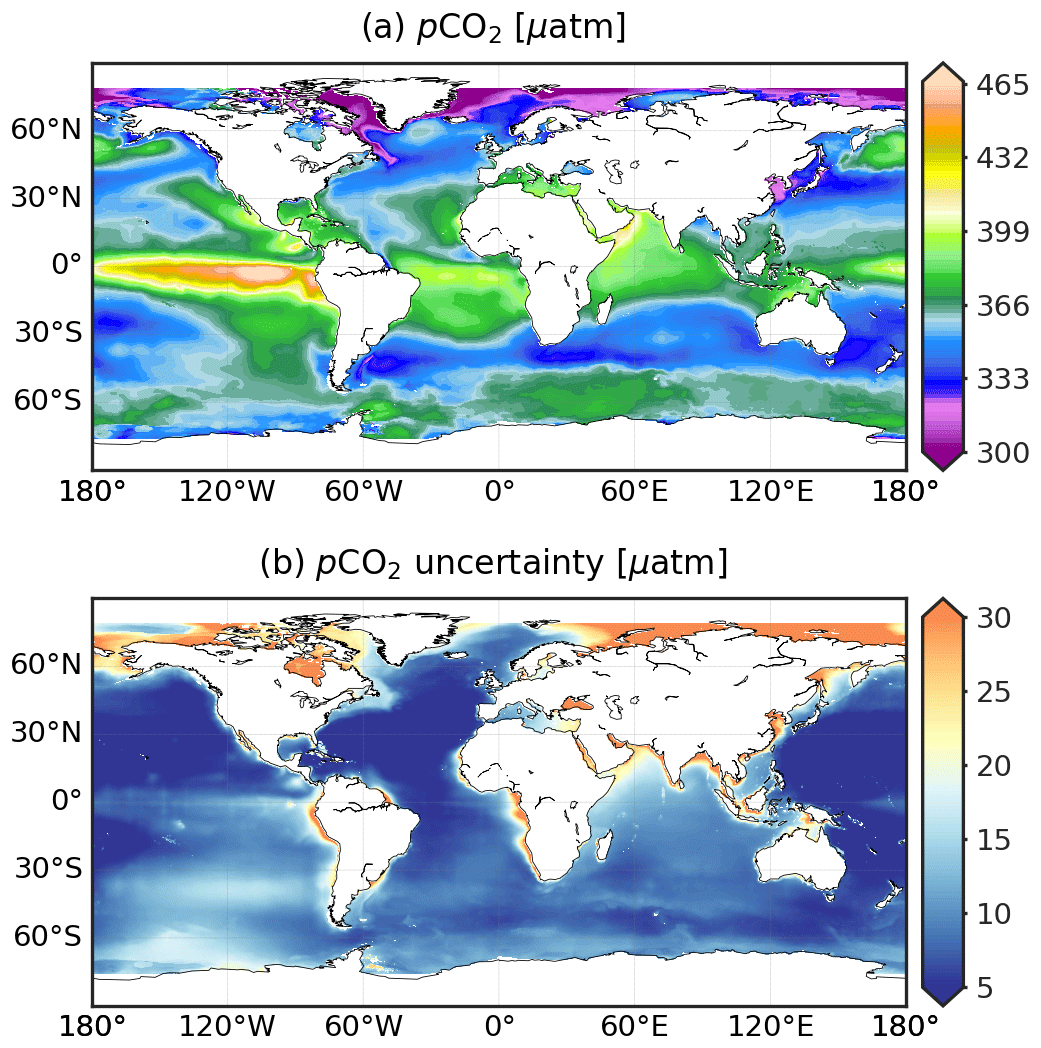
Figure 1CMEMS-LSCE-FFNN pCO2 over the global ocean at a spatial resolution of 0.25∘. Temporal means of the model best estimate and 1σ uncertainty per grid cell over 1985–2021 are calculated by using Eq. (5).
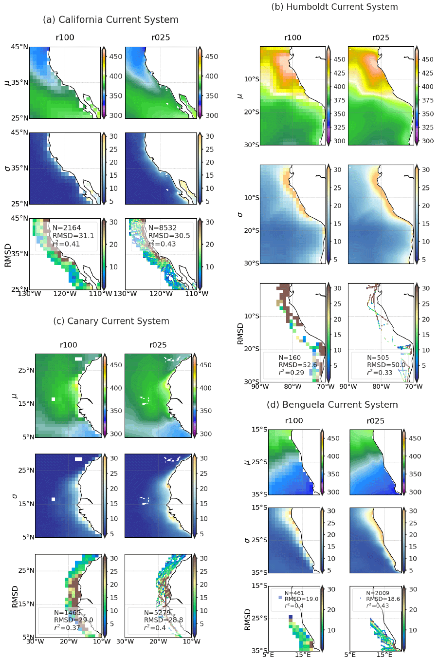
Figure 2Comparison of CMEMS-LSCE-FFNN mapping pCO2 at 1∘ (r100) and 0.25∘ (r025) resolutions over four permanent upwelling regions associated with the eastern boundary currents (California, Humboldt, Canary, and Benguela; see Fig. A1 (A, B, G, and H) for geographical locations). For each region, spatial distributions of pCO2 (μ) and uncertainty (σ) estimates and the coastal–ocean RMSD of pCO2 averaged over 1985–2021 (Eqs. 5 and 10) are shown. Metrics presented in the legend for each of the third rows include the number of coastal–ocean SOCATv2022 data (N), regional RMSD (Eq. 10), and r2 (Eq. 11).
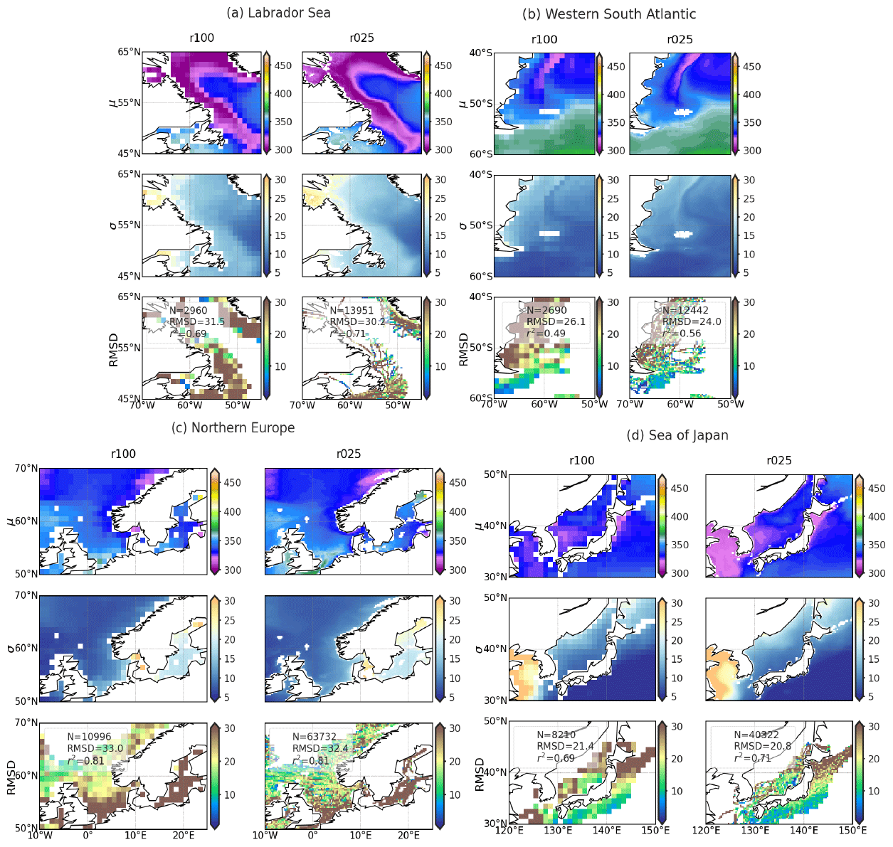
Figure 3Comparison of CMEMS-LSCE-FFNN mapping pCO2 at 1∘ (r100) and 0.25∘ (r025) resolutions over four regions characterized by low pCO2 values (Labrador, western South Atlantic, northern Europe, and Japan; see Fig. A1 (C, E, F, and J) for geographical locations). For each region, spatial distributions of pCO2 (μ) and uncertainty (σ) estimates and the coastal–ocean RMSD of pCO2 averaged over 1985–2021 (Eqs. 5 and 10) are shown. Metrics present in the legend for each of the third rows include the number of coastal–ocean SOCATv2022 data (N), regional RMSD (Eq. 10), and r2 (Eq. 11).
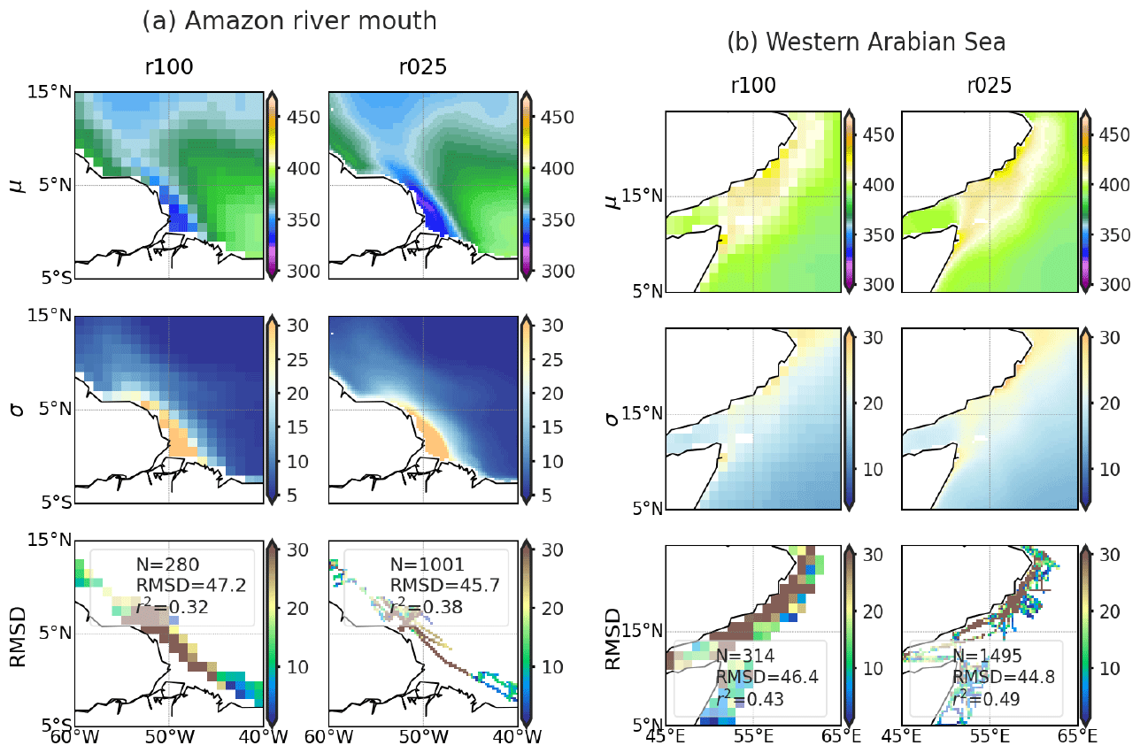
Figure 4Comparison of CMEMS-LSCE-FFNN mapping pCO2 at 1∘ (r100) and 0.25∘ (r025) resolutions over the mouth of the river Amazon and the Western Arabian Sea (see Fig. A1 (D and I) for geographical locations). For each region, spatial distributions of pCO2 (μ) and uncertainty (σ) estimates, and coastal–ocean RMSD of pCO2 averaged over 1985–2021 (Eqs. 5 and 10) are showed. Metrics present in the legend for each of the 3rd row include the number of coastal–ocean SOCATv2022 data (N), regional RMSD (Eq. 10) and r2 (Eq. 11).
Table 3Evaluation statistics for monthly CMEMS-LSCE-FFNN reconstructions of pCO2 at 1∘ (r100) and 0.25∘ (r025) spatial resolutions computed over the period 1985–2021. r100 → 025 and r025 → 100 refer to the versions downscaled or upscaled from the original CMEMS-LSCE-FFNN pCO2 at 1∘ and 0.25∘ resolutions. SOCATv2022 gridded data independent from CMEMS-LSCE-FFNN training are used as benchmarks for model evaluation (see text for details). Statistics including total numbers of data, RMSD (Eq. 10), and r2 (Eq. 11) are reported for both the open ocean (O) and coastal region (C). ∗ Marks results with respect to the primary product proposed in this study.
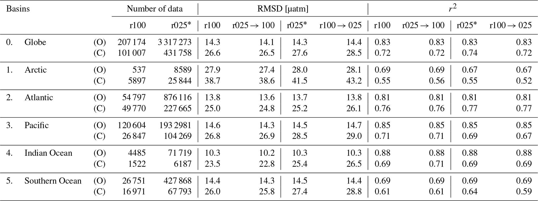
Skill scores of the monthly, 0.25∘ resolution reconstruction are presented in Table 3 (columns marked by an asterisk). The global RMSD (Eq. 10) between the best reconstruction and SOCATv2022r025 pCO2 over the entire period is 14.3 µatm for the open ocean and 27.6 µatm for the coastal ocean. These two model errors are lower than 4 % and 8 % of the global mean pCO2 (Table 6). Moreover, variability present in observation-based data is reproduced by the CMEMS-LSCE-FFNN with high values of r2 (open ocean: 0.83, coast: 0.74). The reconstruction quality is similar among major ocean basins. Spatial distributions of SOCATv2022 data, bias, and RMSD are shown in Figs. A2b and d and A3b, d, f, and h. Estimation skills are low in the ocean basins, with sparse data coverage and significant space–time variability of pCO2 (e.g. Arctic, eastern equatorial Pacific, land–ocean continuum).
Table 3 also presents statistics for the monthly FFNN products of surface ocean pCO2 at spatial resolutions of 0.25∘ (r025) and 1∘ (r100) together with their variants (r100 → 025 and r025 → 100). The latter are, respectively extrapolation and interpolation versions of the original r100 and r025 datasets. We used the Climate Data Operators (CDO) remap operator to regrid FFNN model outputs to a finer or coarser spatial resolution. For compatibility, we compare statistics between
- i.
FFNN(r025) and FFNN(r100 → 025) by using SOCATv2022r025 as evaluation data
- ii.
FFNN(r025 → 100) and FFNN(r100) by using SOCATv2022r100 as evaluation data.
The FFNN(r025) central to this study yields a lower RMSD and a higher correlation to the SOCAT data than the FFNN(r100 → 025). As expected, the improvement in reconstruction skill with higher model resolution is larger over coastal regions than in the open ocean. The FFNN(r025) product after interpolating to a coarser resolution, i.e. FFNN(r025 → 100), agrees with the original 1∘ resolution data product over the whole of the ocean.
The motivation to increase the spatial resolution of the reconstruction is to improve the representation of horizontal gradients of pCO2 at fine scales. Figures 2–4 exemplify spatial distributions for the two reconstructions (r025 and r100) over the coastal–open-ocean continuum. A total of 10 distinct oceanic regions are considered (see Fig. A1a and Table A1 for the 10 locations), and these can be classified into three groups:
-
permanent eastern-boundary-current upwelling systems with relatively high pCO2 (California Current System – CCS, Humboldt Current System – HCS, Canary Current System – CnCS, and Benguela Current System – BCS)
-
regions characterized by low pCO2 values driven by cold water temperatures and strong biological production (Labrador Sea, western South Atlantic, northern Europe, and Sea of Japan)
-
other regions either under the influence of strong river runoff (Amazon mouth) or monsoon-driven upwelling (western Arabian Sea).
The legend of Figs. 2–4 includes regional RMSD and r2 computed between the best estimates of two models and coastal–ocean SOCATv2022r025 data. The coarser spatial resolution product is co-located at the same 0.25∘ grid cells for this analysis. These figures illustrate important discrepancies in pCO2 data density between coastal regions with poorly monitored regions (e.g. HCS, BCS, Amazon mouth) in contrast with areas with higher data coverage (e.g. northern Europe, Sea of Japan).
Over 7 out of the 10 analysed regions with reconstruction at monthly, 0.25∘ resolutions yield RMSDs below 10 % of the global mean of coastal–ocean pCO2 estimates (Table 6) and r2 values higher than 0.3 – e.g. northern Europe (RMSD = 32.4 µatm, r2=0.81), Sea of Japan (RMSD = 20.8 µatm, r2=0.71), and CnCS (RMSD = 28.8 µatm, r2=0.4). The CMEMS-LSCE-FFNN model projections of pCO2 lack skill over the HCS (RMSD = 50.0 µatm, r2=0.33), the region under influence of the Amazon River (RMSD=45.7 µatm, r2=0.38) and the western Arabian Sea (RMSD = 44.8 µatm, r2=0.49). In nearshore sectors of these coastal areas, pCO2 estimates are also subject to a substantial amount of uncertainty (σ > 20 µatm). The lack of model skill reflects the combination of low data density and strong pCO2 gradients driven by multiple underlying physical and biogeochemical processes. The HCS, for instance, is characterized by the highest pCO2 levels (Fig. 2) among the four eastern boundary current systems, with interannual variability being amplified with the El Niño–Southern Oscillation (ENSO) events (Feely et al., 1999; Landschützer et al., 2016). Similarly, high pCO2 levels with substantial seasonal variability are observed over the western Arabian Sea (Fig. 4b), the key driver being monsoonal upwelling (Sabine et al., 2002; Sarma et al., 2013, 2023). In contrast to the two aforementioned coastal regions, high CO2 undersaturation and strong pCO2 gradients (Fig. 4a) are found in the area under the influence of Amazon River discharge (Olivier et al., 2022). Extreme values and large variability of pCO2 challenge any approach to estimating pCO2 data over these regions (Ibánhez et al., 2015; Bakker et al., 2016; Landschützer et al., 2020).
The two FFNN reconstructions (r025 and r100) share similarities in terms of their overall structures of pCO2 over the coastal–open-ocean continuum (Figs. 2–4). However, the higher spatial resolution outperforms its lower-resolution counterpart in reproducing fine-scale features of pCO2 in the transition from nearshore regions to the adjacent open ocean. The increase in model spatial resolution translates into a greater spatial coverage of the continental shelves such as the Labrador Sea, northern Europe, and the Sea of Japan (Fig. 3) and thus an increase in the number of data over the coastal domain. The increase in spatial resolution allows a gain in the prediction probability of pCO2 variations on the order of roughly 2 % over the eastern boundary currents to 7 % over the western South Atlantic (Figs. 2 and 3b).
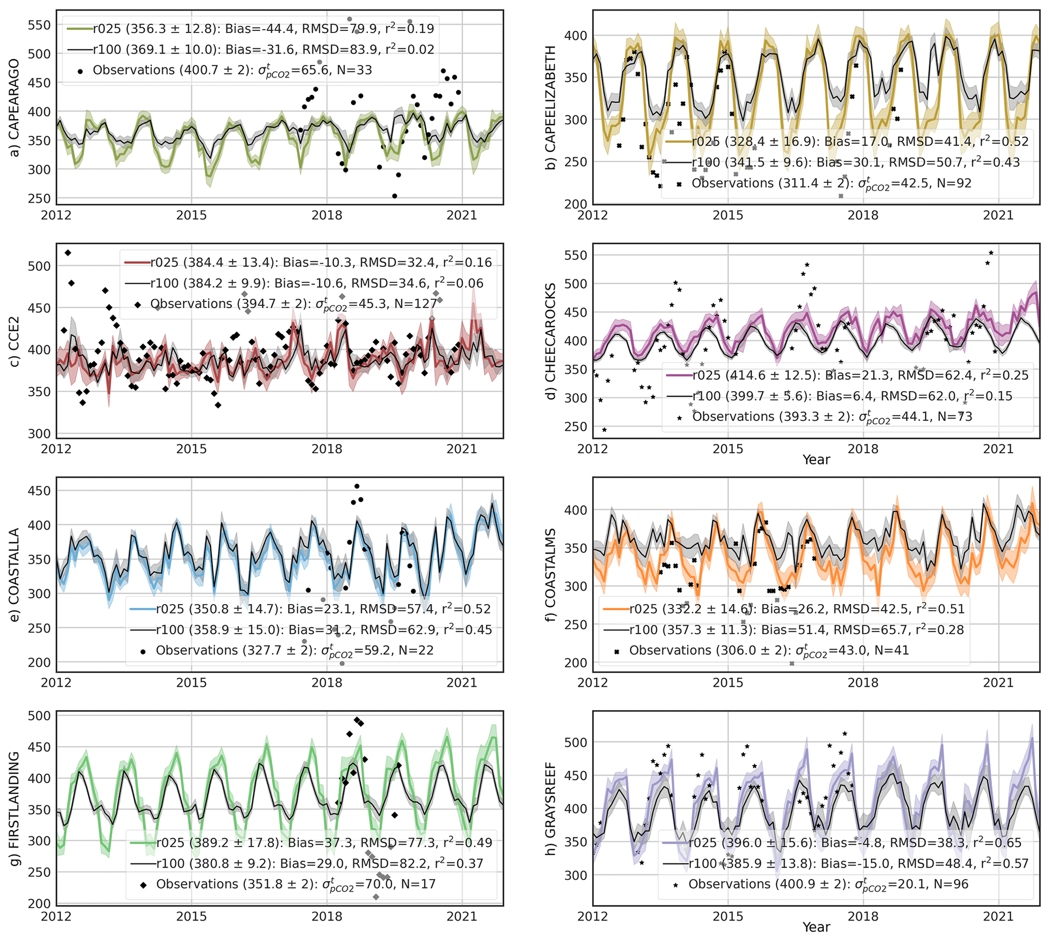
Figure 5Time series of surface ocean pCO2 (µatm) at coastal observing stations (Table A2 and Fig. A1b): model best estimate (curve), 1σ uncertainty (envelope), and monthly average of in situ observations (point). The reconstructed data at 1∘ (r100) and 0.25∘ (r025) resolutions are co-located to in situ observations provided by Sutton et al. (2019). Means of the best estimate and 1σ uncertainty (μ±σ) calculated over the observing time span are shown in brackets. Statistics include number of months with observations (N), bias, RMSD, and r2 computed for the two reconstructions. stands for temporal standard deviation from monthly averages of pCO2 observations.
At the local scale, the reconstruction of in situ pCO2 (Sutton et al., 2019) over the open ocean is on the high order of confidence (Table A3). Low RMSD (between 7.8 and 23.5 µatm) and sustainably high r2 (from 0.45 to 0.98) dominate evaluation statistics over the 18 open-ocean stations. Obviously, CMEMS-LSCE-FFNN has less skill in the coastal sector, and model–observation deviation varies depending on a wide range of pCO2 conditions. However, coastal–ocean RMSD can be smaller than 10 % of the station climatology (e.g. KILONALU, KANEOHE, ALAWAI), and the reproduction availability of temporal variations of pCO2 possibly exceeds 70 % (e.g. SEAK, KODIAK, DABOB). Through Fig. 5, we further assess seasonal to inter-annual variability reproduced at the eight coastal sites (see Fig. A1b and Table A2 for station location) where measurements are available for both pCO2 and pH (analysed in Sect. 5.3) and where they are poorly constrained by the 1∘ reconstruction (Chau et al., 2022b). The temporal variability of pCO2 reported for these time series sites reflects a combination of processes (Sutton et al., 2019), e.g. the California Current System (CAPEARAGO and CCE2), the western coastal upwelling (CAPEELIZABETH), eutrophication enhancing respiration of CO2 (FIRSTLANDING), and multiple stressors on coral reef environments (CHEECAROCKS, GREYREEF). As shown in Fig. 5 (scattered points for observations), time series of coastal pCO2 are still short. The longest time series covers 127 months of pCO2 monitoring since 2010 (CCE2), while the shortest one contributes 17 months with observations (FIRSTLANDING).
Analysing the station time series, we have found that data have been sampled within a few days, with an average offset of about 1 week from the month centre. At these coastal sites, the temporal standard deviation from monthly averages of pCO2 () exceeds analytical errors (2 µatm, Sutton et al., 2019). ranges from 20.1 µatm at GREYREFF to values as large as 65.6 µatm at CAPEARAGO or 70 µatm at FIRSTLANDING. The monthly average of pCO2 might not be adequately represented by discreet samples at sites with a large temporal standard deviation of pCO2. The misfit between the monthly reconstruction and discreet observations is exacerbated in dynamical coastal environments and might explain, in part, the large RMSD of reconstructions of monthly coastal pCO2 (e.g. GREYREEF: 38.3 µatm, CAPEARAGO: 79.9 µatm, FIRSTLANDING: 77.3 µatm) for the r025 reconstruction. The RMSD is mostly lower for the FFNN reconstruction at 0.25∘ resolution compared to the FFNN at 1∘ resolution by 2.2 µatm (CCE2) to 23.2 µatm (COASTALMS). Similarly, r2 increases between 7 %–23 % at higher resolutions. Overall, seasonal to interannual variations of coastal–ocean pCO2 are better reproduced in the reconstruction at 0.25∘ resolution (Fig. 5).
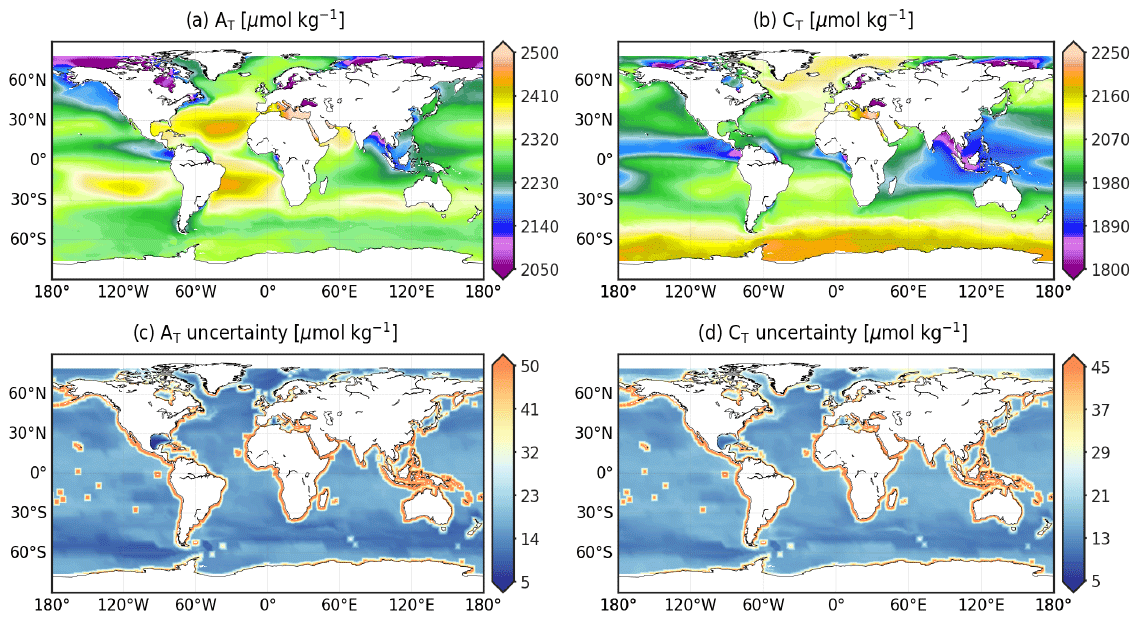
Figure 6CMEMS-LSCE AT and CT over the global ocean at a spatial resolution of 0.25∘. Temporal means of the model best estimate and 1σ uncertainty per grid cell over 1985–2021 are calculated by using (Eq. 5).
5.2 Total alkalinity and dissolved inorganic carbon
This section presents and analyses global ocean surface reconstructions of total alkalinity (AT) and dissolved inorganic carbon (CT) at monthly, 0.25∘ resolutions over 1985–2021. GLODAPv2.2022 bottle data (Sect. 2.2) serve as reference data for model evaluation. Model reconstruction skill is further assessed at the eight Eulerian time series sites: AWIPEV, BATS, DYFAMED, ESTOC, HOT, ICELAND, IRMINGER, and KERFIX (Table 2).
Figure 6 shows spatial distributions of the climatological mean and uncertainty (Eq. 5) for AT and CT. Despite being, in part, influenced by common biological and physical processes, both properties have contrasting distributions due to the strong correlation between surface ocean AT and salinity (Lee et al., 2006; Broullón et al., 2019), as well as the contribution of air–sea gas exchange and biological productivity on surface ocean CT levels (Feely et al., 2001; Takahashi et al., 2014). Over subtropical Atlantic gyres and the Mediterranean Sea, oceanic areas with net evaporation, AT exceeds 2400 µmol kg−1. Total alkalinity falls below 2150 µmol kg−1 in regions where precipitation, river freshwater runoff, or seasonal sea ice melting dilute surface water salinity (e.g. subpolar North Pacific, Arctic, and equatorial river outflows). The distribution of CT is relatively uniform between the Atlantic, Pacific, and Indian Ocean basins but shows pronounced latitudinal gradients. High concentrations of CT are found throughout the Southern Ocean (CT >2100 µmol kg−1) where strong upwelling brings up subsurface water enriched in CO2 and nutrients. The inefficient utilization of nutrients in this high-nutrient, low-chlorophyll region limits the biological drawdown of CT, allowing the massive CT input to be spread horizontally by westerlies (Key et al., 2004; Menviel et al., 2018). Levels of CT below 1900 µmol kg−1 are reconstructed over the equatorial Pacific, the equatorial eastern Atlantic, the eastern Indian Ocean, and coastal areas on the Arctic Ocean. While low CT levels associated with equatorial upwelling reflect gas exchanges across the air–sea interface and enhanced biological production, the interaction between physical and biogeochemical processes at work in the Indian Ocean are less well understood (Takahashi et al., 2014). Low CT levels found close to river mouths reflect outgassing of CO2 across the salinity gradient, as well as enhanced biological uptake fuelled by river nutrient inputs. Representation uncertainty (Fig. 6c and d) associated with monthly alkalinity and CT reconstructions is lower than 20 µmol kg−1 throughout the open ocean. The open-ocean σ-to-μ ratio (Eq. 8) ranges between 0.5–1.5 %, which is relatively small (Fig. A9c and d). CT uncertainty is computed through CO2SYS.v2 error propagation with reconstruction uncertainties of pCO2 and AT set as inputs. The largest values (σ > 30 µmol kg−1) appear nearshore and at surrounding oceanic islands (Fig. 6d). A similar feature is found on the field of AT (Fig. 6c), inherited from input uncertainty associated with the CMEMS salinity product (Fig. A7a).
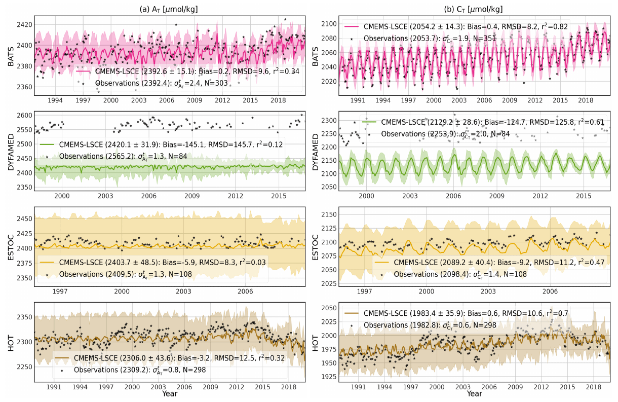
Figure 7Monthly time series of AT and CT at BATS, DYFAMED, ESTOC, and HOT stations (Table 2 and Fig. A1b): model best estimate (curve), 1σ uncertainty (envelope), and monthly average of surface (0–10 m) observations (point). Means of the best estimate and 1σ uncertainty (μ±σ) calculated over the observing time span are shown in brackets if accessible. Statistics include the number of months with observations (N), bias, RMSD, and r2. () stands for the temporal standard deviation from monthly averages of AT (CT) observations.
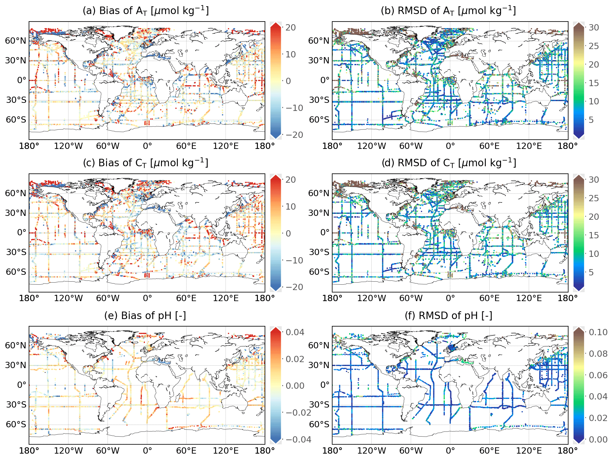
Figure 8Spatial distribution of reconstruction skills for AT, CT, and pH over 1985–2021. Mean model–data difference (bias) and root-mean-square deviation (RMSD) between the reconstruction and GLODAPv2.2022 surface data (0–10 m) at a spatial resolution of 0.25∘. The size of grid cells is scaled upon a better visualization.
Table 4Skill scores computed between CMEMS-LSCE and GLODAPv2.v2022 in AT, CT, and pH over the period 1985–2021. Total numbers of data, RMSD (Eq. 10), and r2 (Eq. 11) are reported for both the open ocean (O) and coastal region (C). Basin identification is shown in Fig. A1.
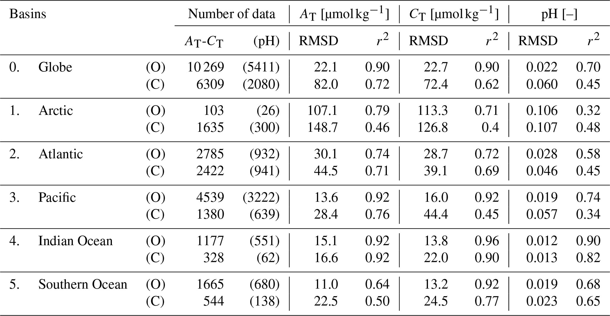
We qualify monthly, 0.25∘ reconstructions of AT and CT with GLODAPv2.2022 data (Lauvset et al., 2022a) for the 37-year period (Table 4 and Fig. 8). The global open-ocean reconstruction scores an RMSD of 22.1 µmol kg−1 and a r2 of 0.9 in AT. Similar numbers are found for CT (RMSD = 22.7 µmol kg−1 and r2=0.9). The model scores the good fit in the open Indian Ocean with RMSD smaller than 15.5 µmol kg−1 and r2 above 0.92 for both variables. The reconstruction deviates from GLODAP data in the western North Atlantic, subpolar North Pacific, tropics, and nearby major rivers (Fig. 8a, b, c, and d).
AT and CT are underestimated in the continental shelves of north Alaska and the northeastern Atlantic, the Mediterranean Sea, the South China Sea, and nearby river plumes (Fig. 8a and c). The Arctic yields the poorest estimations among all the ocean basins with a global RMSD over 100 µmol kg−1 (Table 4). The prediction probability of variability in AT (CT)] is relatively large for the open ocean at 79 % (71 %) but is rather unsatisfying over the coastal ocean (46 % [40 %]). Extrapolating these carbonate variables towards the shore remains challenging, with much higher errors and uncertainty estimates obtained over the continental shelf compared to the open-ocean reconstruction (Table 4, Figs. 6c, d and 8a–d). The coastal–ocean errors are on the order of 10 % of the global mean values of AT and CT (Table 6).
The reconstruction of AT distributions relies on LIAR coefficients fit with GLODAPv2 data (Olsen et al., 2016) covering the years before 2015. These data are also part of the latest version, GLODAPv2.2022 (Lauvset et al., 2022a). They therefore do not correspond to an independent dataset for the evaluation data of the CMEMS-LSCE reconstruction. To accomplish a cross-validation, reconstructions of AT and CT are compared to observations for eight time series stations: AWIPEV, BATS, DYFAMED, ESTOC, HOT, ICELAND, IRMINGER, and KERFIX (see Table 2 and Fig. A1b for data sources and station locations). Table A4 presents the evaluation statistics for all the stations, and Fig. 7 illustrates the comparison between monthly time series of AT and CT extracted from the CMEMS-LSCE datasets and measurements at the four sustained long-term monitoring sites. More than 270 (80) months in the years 1988–2021 (1995–2009 and 1998–2017) include measurements of AT and CT at BATS and HOT (ESTOC and DYFAMED)]. As shown in Table A4, the Arctic site (AWIPEV) provides 52-month data in 2015–2020, while the three other stations sparsely observed AT and CT at the surface layer, resulting in fewer than 30 monthly mean data in 2014–2021 (IRMINGER and ICELAND) and 1992–2018 (KERFIX). The reconstructed time series fit monthly averages of in situ measurements well. Mean estimates of AT (CT) over the observing period are about 2283 (1983) µmol kg−1 at KERFIX (HOT) to 2420 (2219) µmol kg−1 at DYFAMED (AWIPEV). At all the stations (DYFAMED and AWIPEV excepted) and for the two variables, the model–observation misfit is small (Bias <11 µmol kg−1, RMSD < 14 µmol kg−1) relative to the aforementioned mean estimates (Table A4). The highest offset between the CMEMS-LSCE estimation and observations for all the stations is found at DYFAMED (AT: −145.1 µmol kg−1, CT: −124.7 µmol kg−1). DYFAMED provides long-term time series of AT and CT measurements in the northwestern Mediterranean Sea (Fig. A1b). Salinity and alkalinity have substantial values due to the net evaporation (Coppola et al., 2020). The average of AT in the Mediterranean Sea exceeds that for the global ocean by 10 % (Palmiéri et al., 2015). These characteristics set the Mediterranean Sea aside from the ocean basins. Although the bias between reanalysed SSS and observations (Fig. A10) is relatively small, LIAR (Carter et al., 2018) was trained on GLODAPv2 (Olsen et al., 2016), including only a few observations in this area. The distinct relationship between alkalinity and salinity prevailing in the Mediterranean Sea is likely not reproduced by LIAR, leading to an underestimation of AT and a systematic bias in relation to CT at DYFAMED (Fig. 7). ESTOC is located close to the North Atlantic east coast and is under the influence of the Canary Current System (CCS, Fig. A1). Spatial gradients and temporal variability are higher in the CCS (Fig. 2c) compared to BATS and HOT, which are both located in the centre of subtropical gyres. Despite showing good estimates of AT and CT in terms of RMSD at ESTOC, temporal variability of observations is reconstructed with the lowest r2 (Table A4). Particularly, seasonality to multi-year variations in CT are predicted at r2=0.47 for ESTOC compared to r2 > 0.7 for AWIPEV, ICELAND, IRMINGER, BATS, and HOT. Over all the stations, the model underestimates temporal changes in AT (Fig. 7a; BATS: r2=0.33, DYFAMED: r2=0.12, ESTOC: r2=0.03, HOT: r2=0.32), which can be attributed to the large discrepancy in variability between in situ measurements and the CMEMS time series of salinity (Fig. A10a; BATS: r2=0.33, DYFAMED: r2=0.19, ESTOC: r2=0.03, HOT: r2=0.35). Model uncertainty (1σ envelop) of monthly AT and CT estimates (Fig. 7a) is also inflated somewhat proportionally to the CMEMS salinity product uncertainty (Fig. A10a).
5.3 Surface ocean pH and saturation state with respect to carbonate minerals
Surface ocean pH and saturation states with respect to aragonite (Ωar) and calcite (Ωca) are critical indicators used to measure ocean acidification. This section first presents an overall evaluation of these variables. We then introduce estimates involved in the monitoring of ocean acidification in 1985–2021 as an essential application of the CMEMS-LSCE surface ocean carbon product.
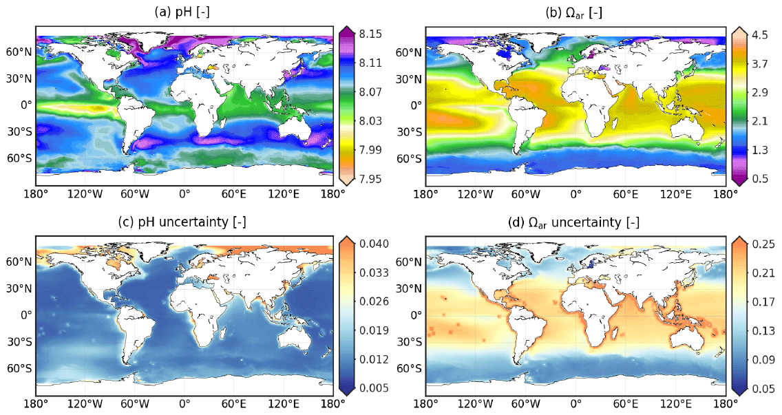
Figure 9CMEMS-LSCE pH and Ωar over the global ocean at a spatial resolution of 0.25∘. Temporal means of the model best estimate and 1σ uncertainty per grid cell over 1985–2021 are calculated by using Eq. 5.
5.3.1 General analysis and evaluation
The spatial distribution of surface ocean pH reported on the scale of total hydrogen ion (H+) is shown in Fig. 9 (the corresponding figure for H+, Fig. A4, is included in the Supplement). Both temporal means of the best model estimate and 1σ uncertainty of pH share spatial patterns with pCO2 (Fig. 1). The variables of pH and pCO2 correlate closely through equilibrium relationships of dissolved CO2 in seawater: an increase in pCO2 generally corresponds to a decrease in pH. The distribution of the climatological mean of pH displays a gradient with latitudes between 8.03 and 8.11 pH units across most of the basins (Fig. 9a). Values of pH below 8 are associated with the upwelling of CO2-rich waters (e.g. eastern equatorial Pacific, western Arabian Sea). pH exceeds 8.15 in sub- and polar cold surface water and in the regions with high biological productivity (e.g. Labrador Sea, Nordic seas, Southern Ocean between 35–50∘ S).
The saturation state of surface ocean waters with respect to calcium carbonate minerals of aragonite and calcite is defined as the ratio of the product of the concentrations of calcium ions (Ca2+) and carbonate ions () to the solubility of the respective calcium carbonate mineral (CaCO3) in surface seawater. With aragonite being the more soluble polymorph, its degree of saturation (Ωar) is smaller than that of calcite (Ωca) (Mucci, 1983). With the exception of this offset, the spatial distributions of their climatological means share common spatial patterns over the global ocean (Figs. 9b and A5a). Surface seawater is generally supersaturated, i.e. Ωar and Ωca greater than 1. The magnitude of surface ocean calcium carbonate saturation state varies with latitude. Values as large as 3.7–4.5 (5–7) for aragonite (calcite) are reconstructed in subtropical and tropical regions. Ωar and Ωca decrease toward the poles. In the Southern Ocean, surface seawater enriched in CO2 from vertical mixing has Ωar (Ωca) values in the range of 1.5–2.1 (2–3.4). Low saturation states are also computed in the Arctic and for waters of upwelling regimes (Fig. 9b). Locally, Ωar drops below 1.3 and even falls under the CaCO3 dissolution threshold of 1 (Gattuso and Hansson, 2011) in the Arctic water runoff and Baltic Sea.
The uncertainty (1σ) of pH, Ωar, and Ωca that propagated the speciation of the CO2 system takes into account the ensemble spread of pCO2 estimates and analysis errors of other variables (Sect. 3.3). Monthly pH uncertainty estimates fall in the 95 % confidence interval of [0.008,0.036], with a global mean value of 0.011. These estimates are in close agreement with the global uncertainty between 0.01–0.022 pH units calculated by Jiang et al. (2019), Iida et al. (2021), and Gregor and Gruber (2021). pH uncertainty is typically larger than 0.03 in the Arctic and in coastal regions (Fig. 9c). In contrast, the reconstructions of Ωar and Ωca are subject to high uncertainty (σ>0.175) between 30∘ S–30∘ N (Fig. 9d and A5b). Regarding the σ-to-μ ratio, mean uncertainty estimates per cell for the saturation states in the (sub-) tropical band are relatively small compared to the mean of the best monthly estimates (Fig. A9e and f). The Arctic and the coastal oceans remain the regions with the largest reconstruction uncertainties for Ωar and Ωca, as well as for pCO2 and pH (Fig. A9a and b). Excluding these regions, R(σ,μ) (Eq. 8) is less than 0.3 % for pH and 8 % for Ωar and Ωca.
The monthly CMEMS-LSCE reconstruction at 0.25∘ resolution is assessed against pH measurements from GLODAPv2.2022 bottle data (Table 2). For the period 1985–2021, the global RMSD amounts to 0.022 (0.060) pH units and r2 scores at 0.70 (0.45) over the open (coastal) ocean (Table 4). Model bias lies within ] pH units, and RMSD is below 0.02 pH units over the open ocean, except for high latitudes over 60∘ (Fig. 8e and f). At the local scale, the time series from Sutton et al. (2019) are used for further evaluation (Tables A2 and A3). There exist many fewer evaluation data for pH than for pCO2, e.g. only 2 months of monitoring pH at COASTALLA and FIRSTLANDING or devoid of pH measurements at equatorial observing systems. CMEMS-LSCE reconstructs pH over the open ocean with rather high scores, e.g. at BOBOA (RMSD = 0.011 and r2=0.71) and KEO (RMSD = 0.014 and r2=0.86). Referring to the eight coastal sites evaluated for pCO2 in Sect. 5.1, RMSD can be as small as 0.035 and 0.04 pH units at CCE2 and GRAYSREEF, while it is over 0.05 pH units at the other stations (e.g. COASTALLA: 0.068, CAPEARAGO: 0.069). Similarly to the pCO2 time series (Fig. 5, Sect. 5.1), pH has been monitored with low sampling frequency (roughly a few days in the tracking month), and the temporal sampling deviation of instantaneous observations from monthly averages () is significant. This temporal sampling uncertainty of pH contributes to the mismatch between model estimates and observations. For example, amounts to 0.048 pH units at CCE2 and 0.020 pH units at GRAYSREEF and reaches the highest values of 0.078 pH units at COASTALLA and 0.086 pH units at CAPEARAGO. Although model–observation misfit and model uncertainty remain high over the coastal sector (see also Figs. 8e and f and 9c), their estimates do not surpass 1 % of the global mean pH (8.082). The reconstructed pH time series reproduce measurement variability with relatively high correlation, r2 in [0.21,0.94], which reinforces the reliability of CMEMS-LSCE pH data.
5.3.2 Ocean acidification: key features from global to local scales
The monthly, 0.25∘ CMEMS-LSCE datasets of pH, Ωar, and Ωca are at the basis of two CMEMS ocean indicators monitoring surface ocean acidification from 1985 to 2021: (1) annual global means and (2) global trend maps.
In Fig. 10, we present annual global means of surface ocean pH and saturation states for aragonite (Ωar). An illustration of calcite (Ωca) is provided in the Appendix (Fig. A13a). For each variable, the calculation of annual global area-weighted means of best estimates (line) and 1σ uncertainties (envelope) follows Eq. 7. The trends reported in the legend result from linear least-squares regression on annual global means of 100 ensembles of the carbonate system variables. These ensembles are generated with a Gaussian distribution having the mean and variance as the best model estimate μ and squared uncertainty (σ2) at monthly time steps and 0.25∘ grid cells, respectively. pH decreases from 8.110 ± 0.017 in 1985 to 8.049 ± 0.014 in 2021 with a descent rate of −0.017 ± 0.004 per decade. Similar trends are found for the surface ocean saturation states with respect to calcium carbonate minerals. The global mean estimates of Ωar (Ωca) amount to 3.141 ± 0.198 (4.807 ± 0.302) and 2.862 ± 0.174 (4.372 ± 0.266) for the open and coastal oceans. The saturation state declines at a rate of −0.080 ± 0.029 per decade with respect to aragonite, while the reduction is steeper for calcite (−0.114 ± 0.045 per decade).
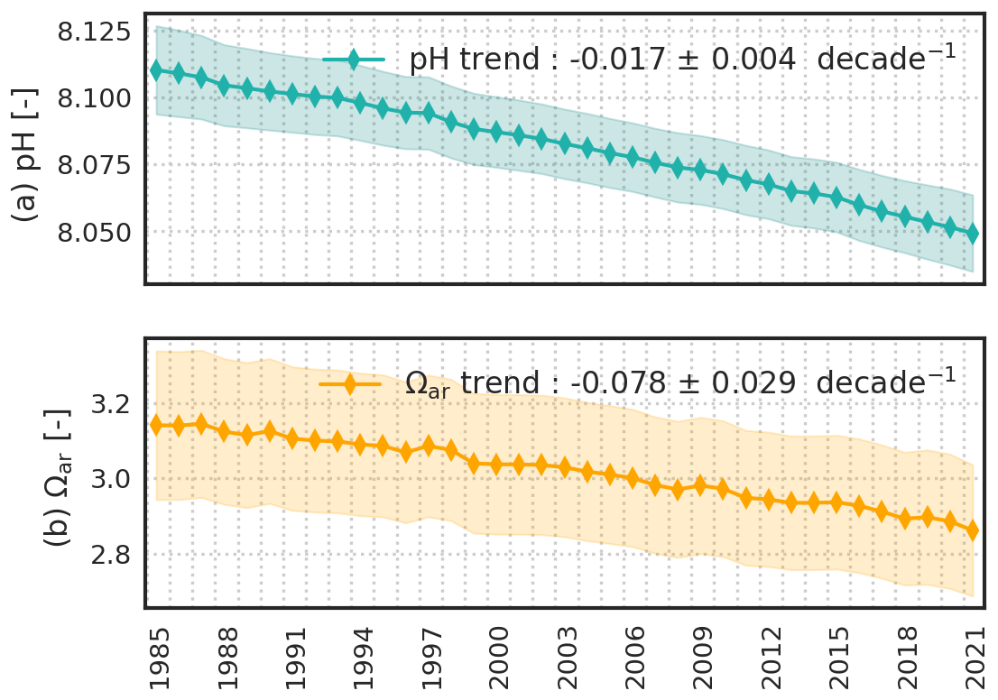
Figure 10Yearly global area-weighted mean of surface seawater pH reported on total scale (a) and surface ocean saturation states with respect to aragonite (b). Global means of the best estimate (μ, plain line) and of uncertainty (σ, envelop) are computed with Eq. (7a). Trend and uncertainty in the legend are computed with linear regressions on the 100-member ensemble of yearly global means for each variable.
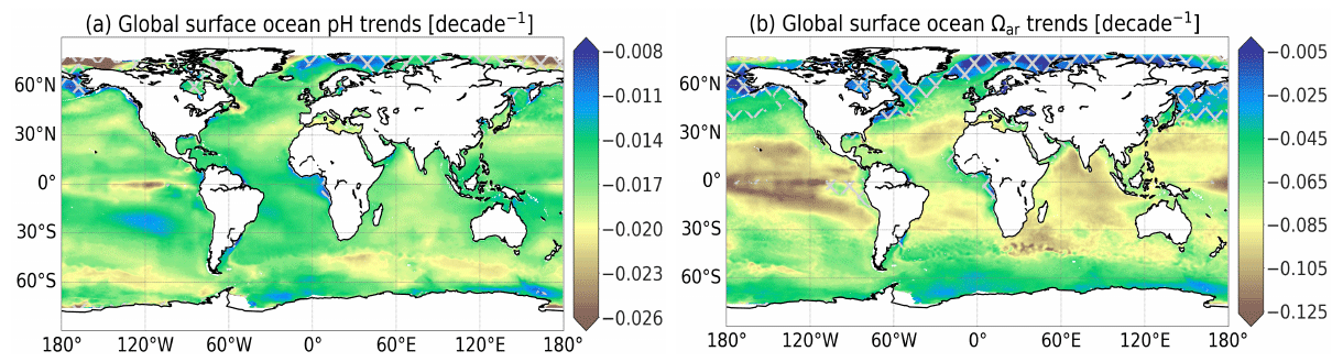
Figure 11Global trend maps of surface seawater pH reported on total scale (a) and surface ocean saturation states with respect to aragonite (b). Linear trend of CMEMS-LSCE pH and Ωar is estimated per 0.25∘ grid cell over 1985–2021. Cross-hatching covers the regions with uncertainty over 10 % (20 %) of pH (Ωar) trend estimates.
Global trend maps of surface ocean pH, Ωar, and Ωca over the entire period are illustrated in Figs. 11 and A13b. Linear least-squares regression is used to estimate secular trends at every 0.25∘ grid cell. The linear fits of each variable against time rely on the 100-member ensemble generated with the best estimates and propagated uncertainties of pH, Ωar, and Ωca (see Fig. A14 for examples). Regression slope and residual standard deviation estimates are defined as linear trend and uncertainty of pH, Ωar, and Ωca. Hatched area represents pH (Ωar and Ωca) trend estimates (μ) with the highest uncertainties (σ), i.e. σ-to-μ ratio (Eq. 8) above 10 % (20 %). These regions include a portion of the Arctic, Antarctic, equatorial Pacific, and coastal ocean (Figs. 11, A11, and A12); 95 % of pH trend estimates over the global ocean are in the range of [] per decade (Fig. 11a). In the broad open ocean of the tropics and subtropics, pH has been declining around −0.018 per decade to −0.012 per decade. Faster decrease rates are found in the Indian Ocean and Southern Ocean, with values between −0.022 and −0.018 per decade. The fastest reductions are computed for the eastern equatorial Pacific and the Arctic with rates exceeding −0.025 per decade. A similar magnitude of pH trends over these regions is also found in (Lauvset et al., 2015; Leseurre et al., 2022; Ma et al., 2023). The spatial distribution of saturation states with respect to calcium carbonate minerals generally shows the opposite latitudinal pattern (Figs. 11b and A13b). The magnitude of Ωar (Ωca) trends over the 30∘ S–30∘ N band can be as large as −0.086 per decade (−0.134 per decade) to the greatest extent of −0.186 per decade (−0.275 per decade) (e.g. eastern equatorial Pacific). Trends of Ωar and Ωca computed in polar and subpolar Northern Hemisphere regions are not significant.
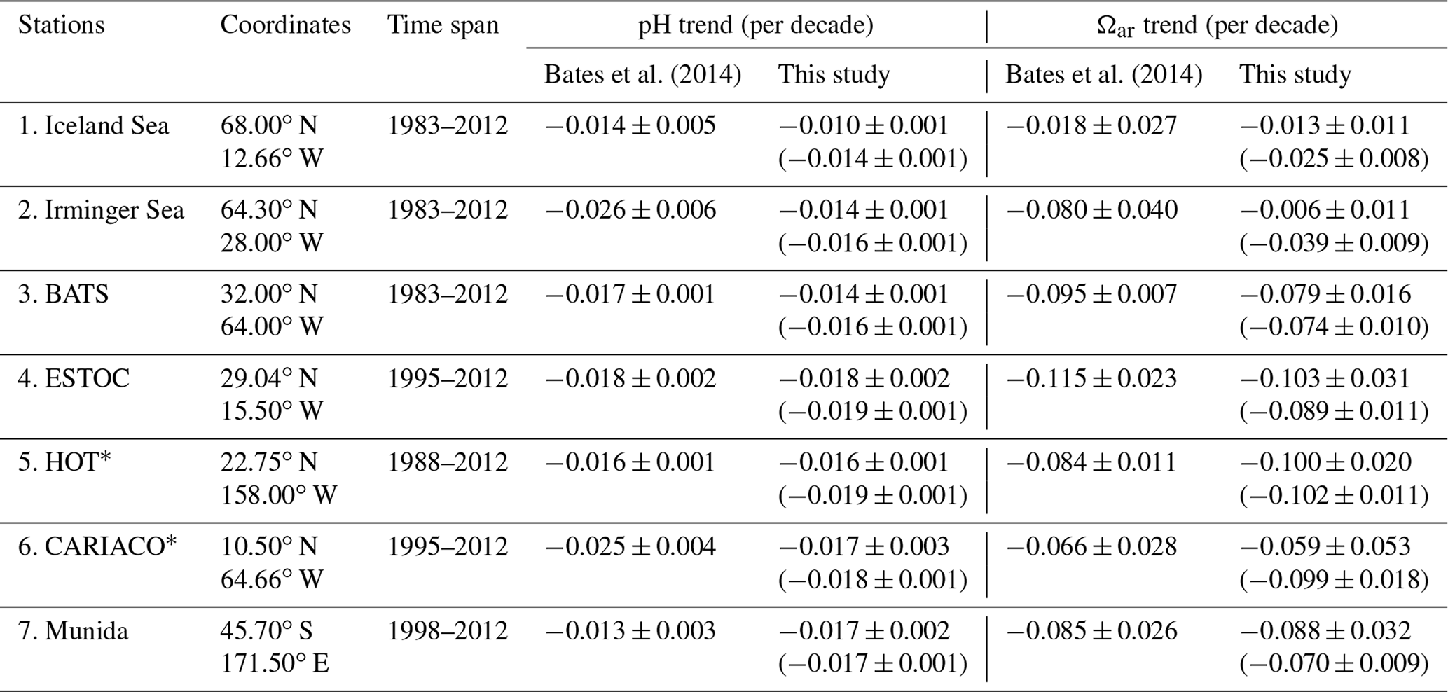
Bates et al. (2014)Bates et al. (2014)Table 5Secular trend estimates of pH and Ωar at seven time series stations (Bates et al., 2014). Trend and uncertainty estimates are reported as μ±σ. Monthly time series in the CMEMS-LSCE datasets are extracted at the grid box nearest to each station location (Fig. A1b). For the first three stations, this study calculates linear trends starting in the year 1985. Brackets show values computed over the full period 1985–2021.
∗ Stations with direct observations of pH.
Trend estimates derived from reconstructions of pH and Ωar are evaluated at seven time series stations (Bates et al., 2014) in Table 5. Time series locations are shown in Fig. A1b. With the exception of CARIACO and HOT, for which pH measurements are available, long-term trend estimates by Bates et al. (2014) rely on time series of pH and Ωar calculated via speciation from measurements of AT and CT. The 100-member ensembles of monthly time series of pH and Ωar are extracted from the 0.25∘ grid box nearest to each monitoring station. Linear least-squares regression is then used to infer estimates of their secular trends and associated uncertainties (see Fig. A14 for illustration). Trend estimates derived from CMEMS-LSCE reconstructions at HOT, BATS, ESTOC, and Munida are in line with previous studies for both pH and Ωar (Dore et al., 2009; González-Dávila and Santana-Casiano, 2009; Bates et al., 2014). The magnitude of the trend estimate at the Irminger Sea for 1985–2012 (pH: −0.014 ± 0.001 per decade, Ωar: −0.006 ± 0.011 per decade) is smaller than that determined by Bates et al. (2014). However, the CMEMS-LSCE pH trend is consistent with the estimate by Pérez et al. (2021) (−0.017 ± 0.002 per decade). Moreover, 1σ uncertainty reported for both pH and Ωar trend estimates by Bates et al. (2014) is large at this station (pH: −0.025 ± 0.006 per decade, Ωar: −0.080 ± 0.040 per decade), highlighting the associated uncertainty. Long-term trends of pH and Ωar are also underestimated at the Iceland Sea monitoring site, but the bias is not as large as at the Irminger Sea (Table 5). Low data-sampling frequency at these two stations (Table 1, Bates et al., 2014) could be on account of trend estimate deviation. At CARIACO, the CMEMS-LSCE time series yields a decrease in Ωar of −0.059 ± 0.053 per decade, relatively close to Bates et al. (2014) (−0.066 ± 0.028 per decade). The decrease in pH derived from CMEMS-LSCE is, however, larger than in Bates et al. (2014).
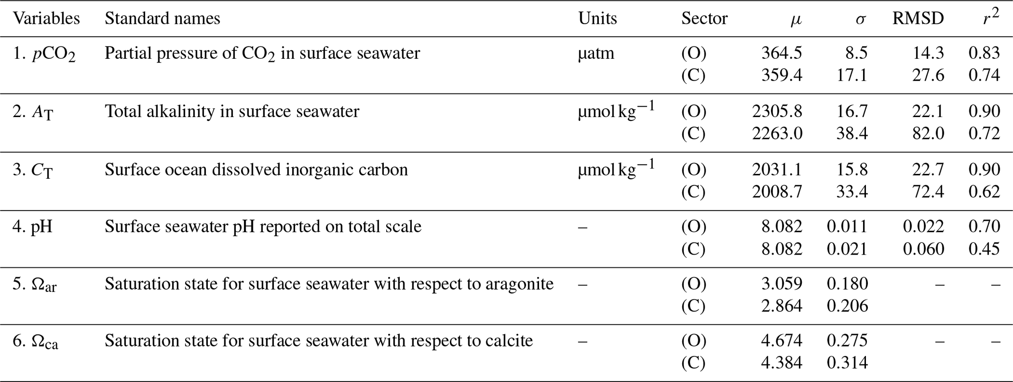
Table 6Summary of global evaluation statistics for CMEMS-LSCE surface ocean carbonate system datasets at monthly, 0.25∘ resolutions over the period 1985–2021. μ and σ stand for the global area-weighted means of monthly best estimates and 1σ uncertainties for each variable (Eq. 7). RMSD (Eq. 10) and r2 (Eq. 11) are computed with SOCATv2022 for pCO2 and GLODAPv2.2022 for pH, AT, and CT. The division between the coastal (C) and open (O) oceans is at 400 km distance from the shore line (Fig. A1a).
The CMEMS-LSCE datasets (netCDF format) of six carbonate system variables have been delivered to the European Copernicus Marine Environment Monitoring Service (CMEMS; product ID: MULTIOBS_GLO_BIO_CARBON_SURFACE_REP_015_008, DOI: https://doi.org/10.48670/moi-00047). The high-resolution data product described in this paper can be accessed via the repository under the following data DOI: https://doi.org/10.14768/a2f0891b-763a-49e9-af1b-78ed78b16982 (Chau et al., 2023).
This study presents the CMEMS-LSCE product, a dataset of six carbonate system variables (Table 6) covering the global surface ocean at a spatial resolution of 0.25∘ for every month in the period 1985–2021 (444 months). Datasets of individual carbonate system variables are built on the combination of the three methods. First, we adapt an ensemble of 100 feed-forward neural network models (CMEMS-LSCE-FFNN; Chau et al., 2022b) to estimate surface ocean partial pressure of CO2 (pCO2) at the pre-defined data resolution. Second, the high-resolution total alkalinity (AT) reconstruction is obtained by using locally interpolated alkalinity regression (LIAR; Carter et al., 2016, 2018). Finally, surface ocean pH, total dissolved inorganic carbon (CT), and saturation states with respect to aragonite (Ωar) and calcite (Ωca) are calculated with the carbonate system speciation software (CO2SYS.v2; Lewis and Wallace, 1998; Van Heuven et al., 2011; Orr et al., 2018), given the global monthly reconstructions of pCO2 and AT and other environmental input data (Sect. 3). Results are 2D fields of the best estimate and associated uncertainty (1σ) of carbonate system variables available at each grid box of 1 month × 0.25∘ × 0.25∘; 1σ uncertainty is referred to as the ensemble standard deviation of 100 FFNN outputs for pCO2 while it is propagated through the processing chain of LIAR and CO2SYS.v2, taking into account different uncertainty sources of input parameters for other variables.
Multiple observation-based datasets, which are not used for the CMEMS-LSCE reconstructions at monthly and 0.25∘ resolutions, serve as benchmarks in the assessments of product quality from global to local scales (e.g. Tables 3, 4, and A3; Figs. 2–5, 7, and 8). A summary of the primary statistics for all the six carbonate variables is presented in Table 6. Over the full period of 1985–2021, CMEMS-LSCE yields global RMSDs of 14.3 µatm and 27.6 µatm in comparison with SOCATv2022 pCO2 for the open and coastal oceans, respectively. Temporal variability of observation-based data is well reproduced, with r2 of 0.83 for the open ocean and 0.74 for the coastal domain. In comparison to CMEMS-LSCE at monthly and 1∘ resolutions (Chau et al., 2022b), the reconstructions over coastal areas are improved at higher resolution. The monthly, 0.25∘ reconstruction outperforms its 1∘ counterpart in reproducing horizontal and temporal gradients of pCO2 over a variety of oceanic regions, as well as at nearshore time series stations (Figs. 2–5). Evaluations with GLODAPv2022 bottle data and time series stations results in good reconstruction skills for AT, CT, and pH at monthly and 0.25∘ resolutions (Tables 4 and A3, Figs. 7 and 8). At the global scale, the open-ocean reconstruction scores an RMSD smaller than 23 µmol kg−1 and a r2 of 0.9 in AT and CT. The model–observation deviation is higher in the coastal zone. However, it does not exceed 5 % of the global mean values, and r2 is above 0.6 for both coastal AT and CT. Regarding pH, the CMEMS-LSCE reconstruction provides estimates with RMSD = 0.022 (0.060) and r2=0.7 (0.45) over the open (coastal) ocean. From the statistics in Tables 3 and 4, the Indian Ocean and the Southern Ocean have poor data density (Fig. A2) but generally show the best global reconstruction among the ocean basins. Thus, model evaluation with different numbers of observation data might not reflect a fair comparison of skill scores (e.g. RMSD and r2) between regions. Data density is much higher in the Arctic, Atlantic, and Pacific than in the Indian and Southern oceans. The increased data density reveals stronger spatio-temporal variability, for instance, related to coastal dynamics or upwelling than what is resolved in the two latter basins. RMSD and r2 computed on the lower data variability result in better model scores.
The spatial distribution of long-term mean 1σ uncertainty estimates (Figs. 1b, 6c, and d and 9c and d) indicates higher confidence levels for open-ocean estimates than over the coastal sector. The evaluation of temporal mean 1σ uncertainty estimates relative to climatological mean values μ (Figs. 1a, 6a and b, and 9a and b) results in σ-to-μ ratios (Eq. 8) below 5 % and 8 % for pCO2 and Ωar, 2 % for AT and CT, and 0.4 % for pH over the open ocean (Fig. A9). The σ-to-μ ratio reaches values as high as 10 % to 20 % for pCO2 and Ωar in the coastal domain. The global means of open-ocean 1σ uncertainty estimates (Eq. 7a) for CMEMS-LSCE pCO2 (8.5 µatm), AT (16.7 µmol kg−1), CT (15.8 µmol kg−1), pH (0.011), and Ωar (0.180) are in line with those reported by previous studies despite being derived from different statistics. For instance, Iida et al. (2021) calculated 1σ uncertainty based on the median absolute deviation of regression model fits from open-ocean observations. Their approach yielded global σ averages of 17.8 µatm, 11.5 µmol kg−1, 0.018, and 0.110 for pCO2, normalized CT, pH, and Ωar, respectively. In Gregor and Gruber (2021), the authors propagated the sum squared errors (global RMSD and measurement uncertainties) of pCO2 (15 µatm) and AT (22 µmol kg−1), obtaining global uncertainty estimates of 19 µmol kg−1 in CT and 0.022 in pH. Mean uncertainty estimates over the coastal region are on the order of 2-fold, computed for the open ocean for these four variables (Table 6), corroborating results by Gregor and Gruber (2021) (Fig. 7).
Our high-resolution carbon data product opens the door to various analyses of the marine carbonate system from the global to local scale. This study exemplifies an application of the data for monitoring ocean acidification over recent years. The monitoring indicators derived from the monthly, 0.25∘ surface ocean CMEMS-LSCE product consist of (1) yearly global means of surface ocean pH and saturation states with respect to aragonite Ωar and calcite Ωca and (2) global maps of multi-annual trends of surface ocean pH, Ωar, and Ωca (Figs. 10, 11, and A13). In 1985, the global mean surface ocean pH was 8.110 ± 0.017. It was 8.049 ± 0.014 in 2021 (Fig. 10a). Over the same 37-year time period, Ωar decreased from 3.141 ± 0.198 to 2.862 ± 0.174 (Fig. 10b). The rate of decline of surface ocean pH and Ωar was, respectively, −0.017 ± 0.004 per decade and −0.080 ± 0.029 per decade from 1985 (see also results for Ωca in Sect. 5.3.2). Estimates of pH trend lie between [] per decade across most of the open ocean (Fig. 11a). In general, surface ocean pH decreased more rapidly in the Indian Ocean and Southern Ocean than in the tropics and subtropics. These findings are in close agreement with the suggestions by Lauvset et al. (2015) and Ma et al. (2023), but future studies would need to include analyses of underlying drivers to provide insight into regional differences in pH changes. By contrast, the greatest reduction in surface ocean saturation states (Fig. 11b) was computed for the two latter regions. The global trend maps of pH and Ωar highlight the eastern equatorial Pacific as one of the vulnerable regions with respect to ocean acidification. In this area, the decline rate of pH exceeds −0.025 per decade and −0.186 per decade for Ωar. The comparison of multi-annual trends of pH and Ωar at time series stations (Table 5 and Fig. A14) highlighted the consistency between CMEMS-LSCE estimates and previous studies (Dore et al., 2009; González-Dávila and Santana-Casiano, 2009; Bates et al., 2014; Pérez et al., 2021). For most of these sites, the trends evaluated for 1985–2021 are greater than those relative to the sub-period before the year 2012. The faster rate of ocean acidification over the full period compared to pre-2012 probably reflects a steeper acceleration in ocean uptake of anthropogenic CO2 in the last decade. The global maps of CMEMS-LSCE pH, Ω, and their trend estimates would be potential indicators for ocean acidification along with the SDG 14.3.1 – namely “average marine acidity (pH) measured at an agreed suite of representative sampling stations” (https://sdgs.un.org/goals/goal14, last access: 31 July 2023).
The production chain of CMEMS-LSCE carbonate system variables will be maintained, and further improvements with the aim of reducing model–observation misfit and improving the quantification of model uncertainty are on the way forward. Being at the core of the chain, model upgrades of CMEMS-LSCE-FFNN will be tackled first. At this time, SOCAT does not provide open-ocean data of CO2 fugacity gridded at monthly, 0.25∘ resolutions. Our ensemble-based approach thus draws on two SOCATv2022 data sources: a downscaled version of the 1∘ open-ocean data and the 0.25∘ coastal–ocean data (see Sect. 2.1). Open-ocean SOCAT datasets gridded at finer regular resolutions (if accessible) will be updated to gain more accuracy in our model fitting. Selections of data products for predictors needed for model input are equally important. For instance, the CMEMS SSS product used here results in a globally good reconstruction of total alkalinity (Table 4). However, the temporal variability in CMEMS SSS data does not match that in observations (Fig. A10), and this feature is retained in time series of total alkalinity (Fig. 7). Despite our best efforts in determining the overall product uncertainty in estimates of carbonate system variables, part of the input uncertainty is still not taken into account or only partially quantified due to a lack of time–space-varying uncertainty fields associated with predictor variables (e.g. SSH, Chl a, MLD, nutrient concentrations). Moreover, temporal sampling bias in pCO2 and pH is likely to contribute to deviations between observations and model output (Fig. 5 and Table A3). The total analytical error uncertainty should be considered with great care during reconstruction and model output evaluation.
The CMEMS-LSCE approach leads as the first series of long-term reconstructions of pCO2, pH, AT, CT, Ωca, and Ωar extending seamlessly from the global open ocean to coastal regions at monthly, 0.25∘ resolutions. Future-use cases recommended for this high-resolution product include (1) estimation of monthly to interannual variations, long-term trends of carbonate system variables, and air–sea CO2 exchanges at the surface layer from the local scale to large ocean basins; (2) analyses of interactions between these variables and the effects of other physical and biogeochemical factors on ocean acidification and changes in the marine carbonate system; (3) assessments of horizontal and temporal gradients of carbonate system variables in the coastal–open-ocean continuum; (4) evaluation or combination with other model- or observation-based products (e.g. Biogeochemistry Argo, Southern Ocean Carbon and Climate Observations and Modeling); and (5) improvements in coastal reconstructions based on observation system simulation experiments (e.g. with finer spatio-temporal model resolutions). The CMEMS-FFNN surface ocean carbon product at monthly, 0.25∘ resolutions will be accessible through the CMEMS data portal (see Sect. 6).
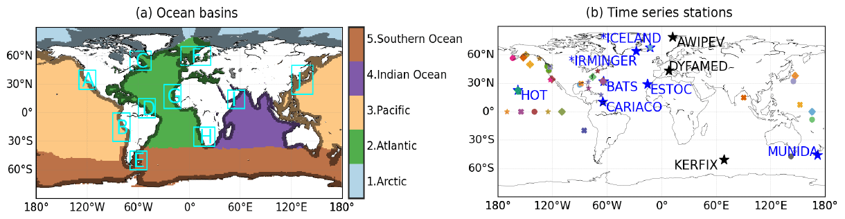
Figure A1(a) Ocean basins (https://github.com/RECCAP2-ocean/RECCAP2-shared-resources/tree/master/data/regions, last access: 11 July 2022): coastal mask (grey, approximately 400 km from the shoreline) and feature regions analysed in this study (cyan box, Table A1). (b) Location of time series stations recording in situ observations used in data evaluation (Table 2): blue stars for ocean acidification (Bates et al., 2014), black stars for AT and CT (Metzl and Lo Monaco, 1998; Coppola et al., 2021; Gattuso et al., 2023a), and other coloured scattered objects for pCO2 and pH (Sutton et al., 2019). Asterisk (∗) marks the two stations with additional AT and CT observations (Olafsson et al., 2010) available for assessments.
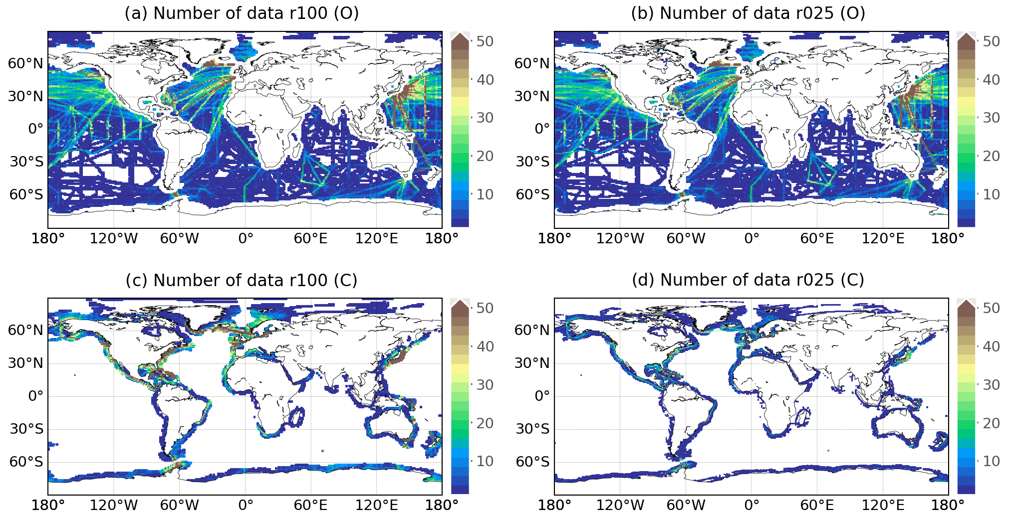
Figure A2Spatial distribution of total months in 1985–2021 containing SOCATv2022 gridded data: (a, c) 1∘ data product (r100), (b, d) 0.25∘ data product (r025). Open-ocean data (O) in each 0.25∘ grid box are created by setting conservatively the open-ocean SOCATv2022 data at the 1∘ grid box containing it. The coastal–ocean SOCATv2022 data (C) are assigned within 400 km from the shoreline (Fig. A1a).
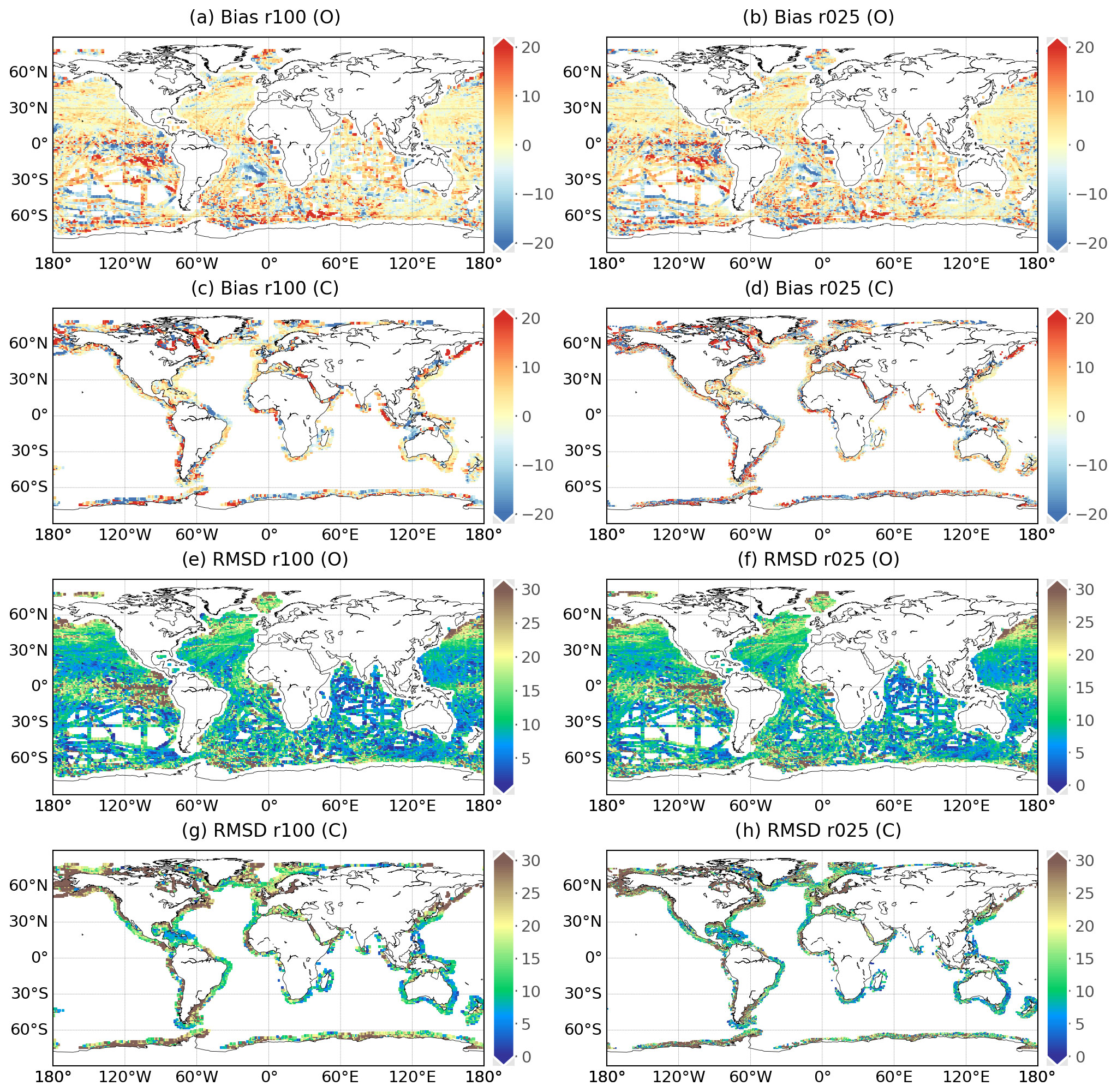
Figure A3Global maps of mean model–data difference (bias, a–d) and root-mean-square deviation (RMSD; e–h) between the reconstruction and SOCATv2022 pCO2 (µ atm) over 1985–2021. (a, c, e, g) CMEM-LSCE-FFNN with a resolution of 1∘ (r100); (b, d, f, h) CMEM-LSCE-FFNN with a resolution of 0.25∘ (r025). Open-ocean data (O) in each 0.25∘ grid box used for evaluation are created by setting conservatively the open-ocean SOCATv2022 data value at the 1∘ grid box containing it. Coastal–ocean data (C) are extracted from each of the two SOCATv2022 gridded data products.
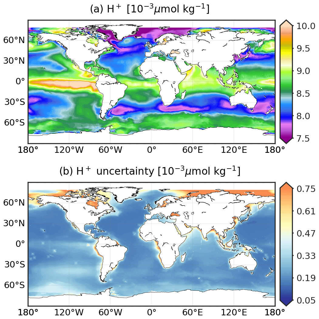
Figure A4CMEMS-LSCE H+ over the global ocean at a spatial resolution of 0.25∘. Temporal means of the model best estimate and 1σ uncertainty per grid cell over 1985–2021 are calculated by using Eq. (5).
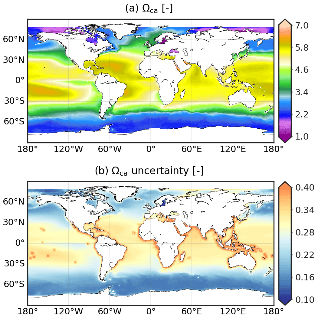
Figure A5CMEMS-LSCE Ωca over the global ocean at a spatial resolution of 0.25∘. Temporal means of the model best estimate and 1σ uncertainty per grid cell over 1985–2021 are calculated by using Eq. (5).
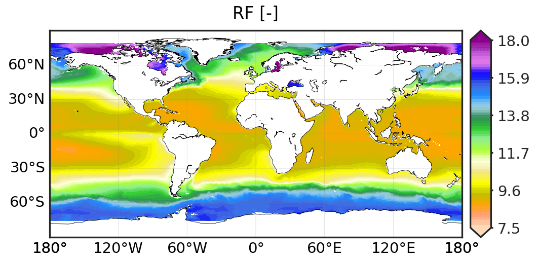
Figure A6CMEMS-LSCE Revelle factor (RF) over the global ocean at a spatial resolution of 0.25∘. Temporal means of the model best estimate per grid cell over 1985–2021 are calculated by using Eq. (5).
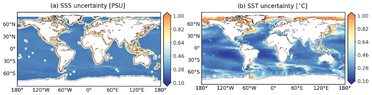
Figure A7Spatial distribution of CMEMS SSS and SST product uncertainty over the global ocean at a spatial resolution of 0.25∘; 1σ uncertainty is computed per grid cell by using Eq. (5) over 1985–2021.
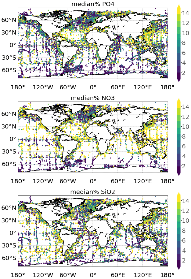
Figure A8Median percentage of analysis error uncertainty against climatological mean of surface WOA18 nutrient data: phosphate (PO4), nitrate (NO3), and silicate (SiO2).
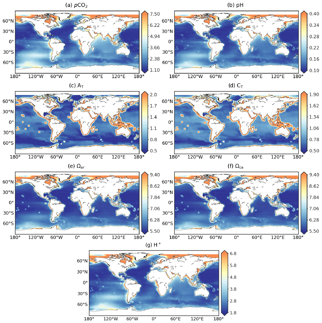
Figure A9Spatial distribution of R(σ,μ) [%] (Eq 8), i.e. the ratio of model uncertainty (σ) against model best estimate (μ).
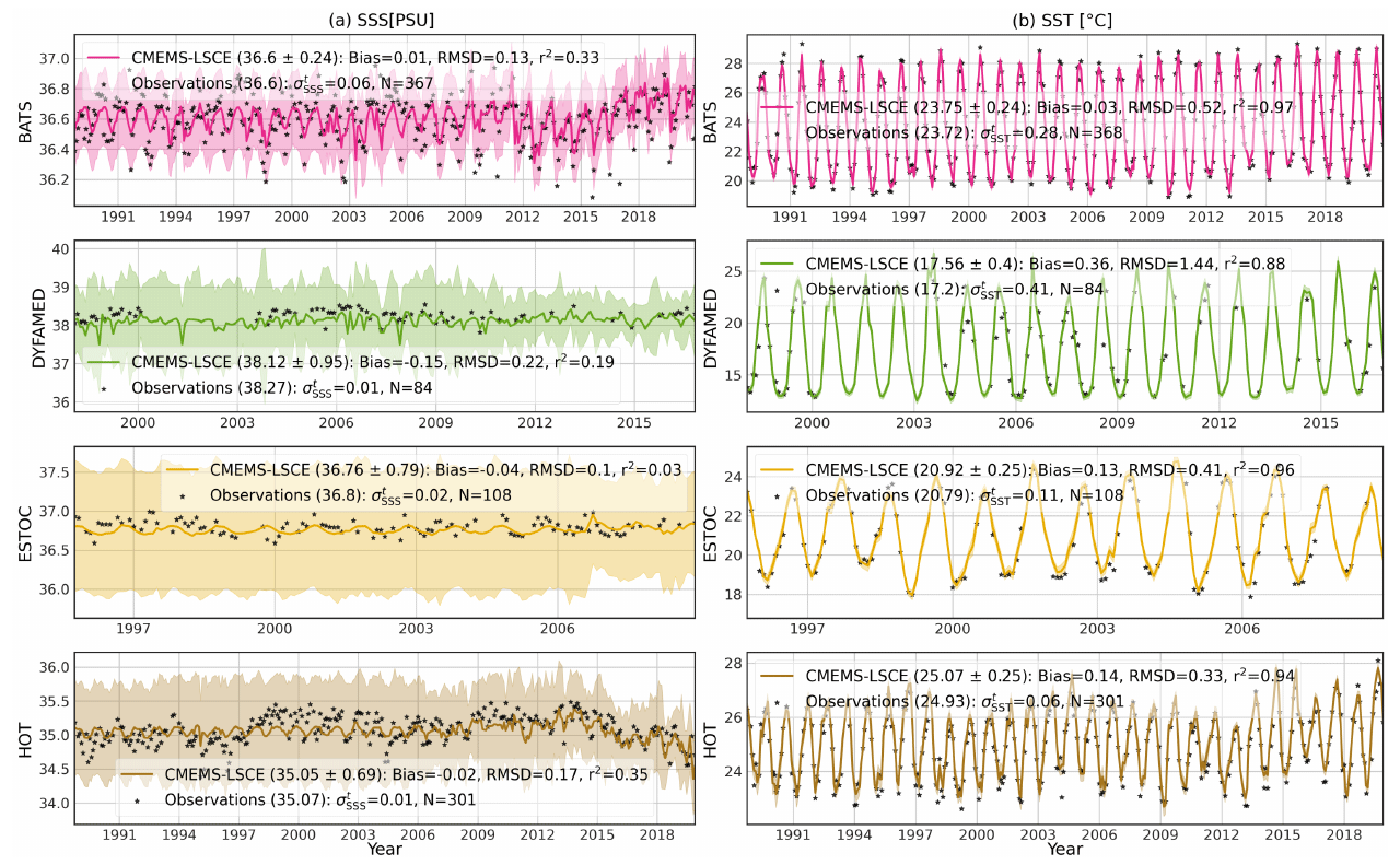
Figure A10Monthly time series of SSS and SST at BATS, DYFAMED, ESTOC, and HOT stations (Table 2 and Fig. A1b): CMEMS data (curve), 1σ uncertainty (envelope), and monthly average of observations (point). Means of CMEMS data and 1σ uncertainty (μ±σ) calculated over the observation time span are shown in brackets if accessible. Statistics include the number of months with observations (N), bias, RMSD, and r2; () stands for temporal standard deviation from monthly averages of SSS and SST observations. Temporal variations in SSS observations are poorly described in the CMEMS SSS time series (Table 1) used in CMEMS-LSCE reconstructions.
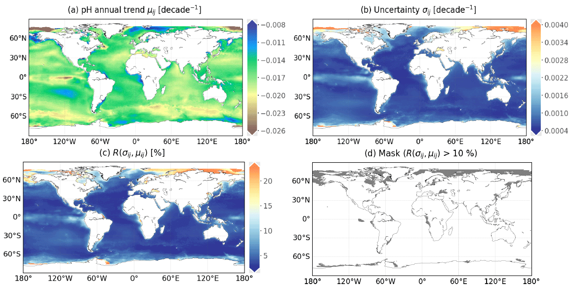
Figure A11(a) Global surface seawater pH trend over the period 1985–2021, (b) 1σ uncertainties associated with trend estimates, (c) σ-to-μ ratio R(σ,μ) [%] (Eq. 8) between uncertainty estimates (b) and the best trend estimates (a), and (d) mask applied over the regions where .
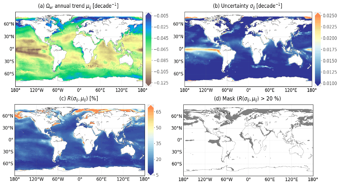
Figure A12(a) Global surface seawater Ωar trend over the period 1985–2021, (b) 1σ uncertainties associated with trend estimates, (c) σ-to-μ ratio R(σ,μ) [%] (Eq. 8) between uncertainty estimates (b) and the best trend estimates (a), and (d) mask applied over the regions where .
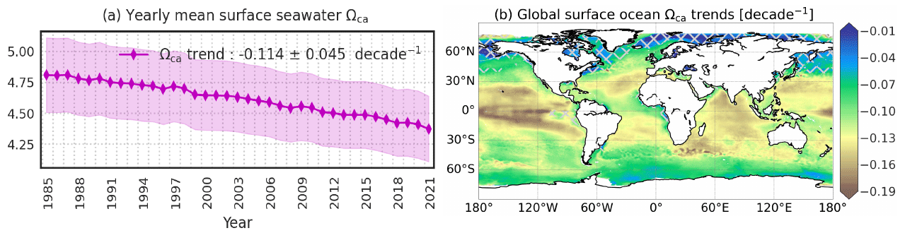
Figure A13(a) Yearly global area-weighted mean of surface ocean saturation states with respect to calcite (Ωca): global means of the best estimate (μ, plain line) and uncertainty (σ, envelop) are computed with Eq. (7a). (b) Global trend maps of Ωca over 1985–2021: cross-hatching covers the regions with uncertainty of a trend estimate over 20 % of the trend value.
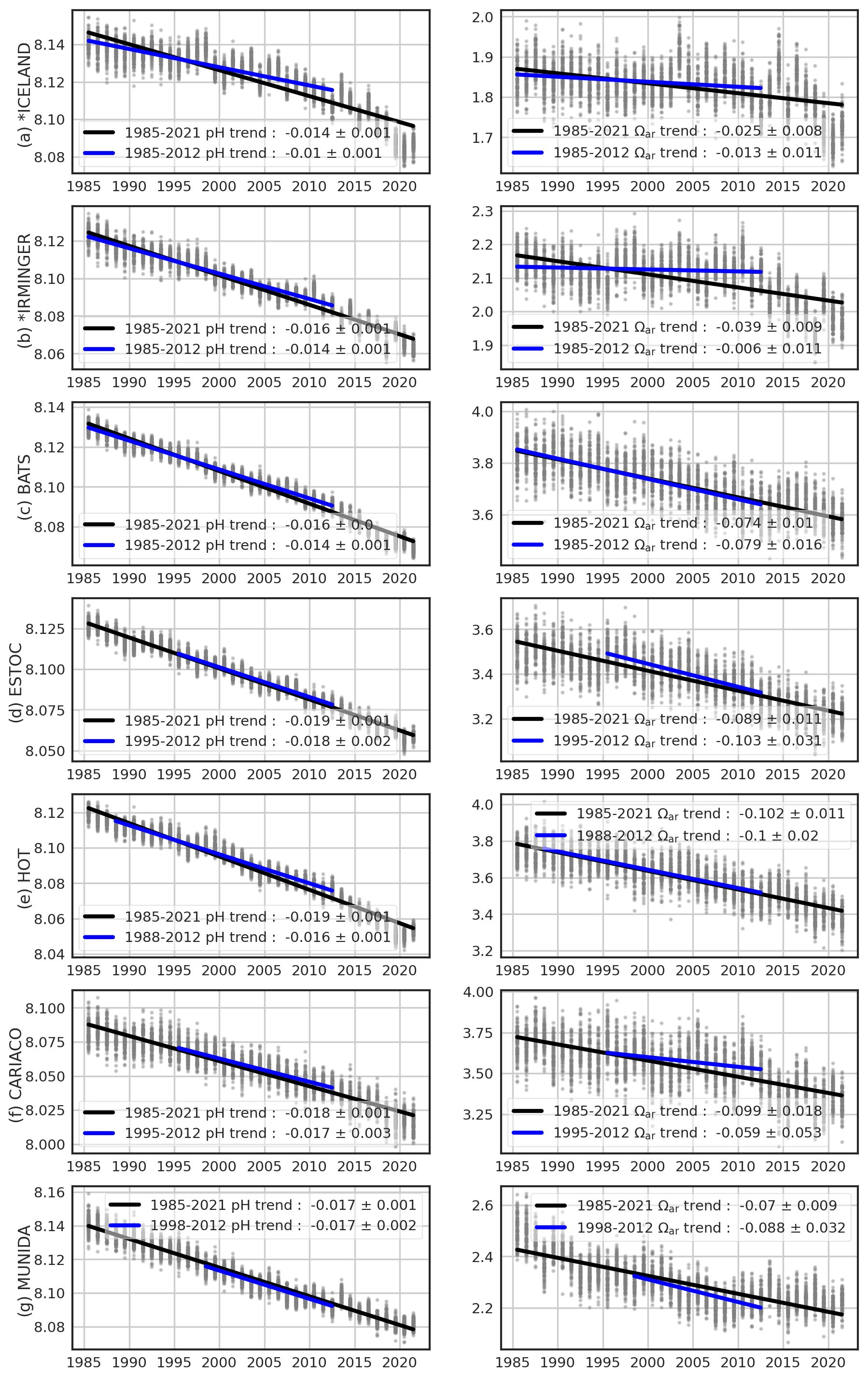
Figure A14Linear trend estimates (per decade) learnt on 100-member ensembles (grey points) of yearly mean time series of pH and Ωar at different stations (Bates et al., 2014). μ±σ present linear slope and residual standard deviation. Black or blue lines stand for linear fits over the full or sub-period in 1985–2021 (see Table 5 for comparison).
Table A1Information of feature regions analysed in this study (Fig. A1a – cyan boxes).
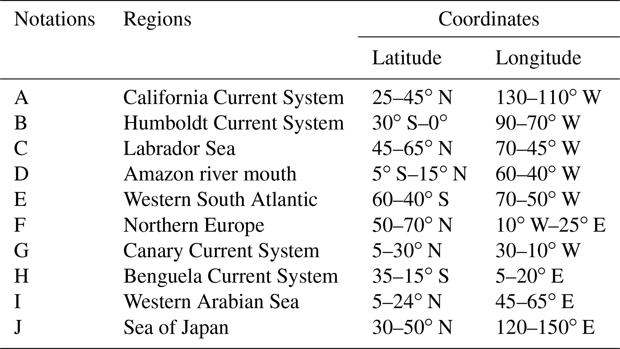
Table A2Information of moored time series of surface–ocean pCO2 and pH observations (Sutton et al., 2019).
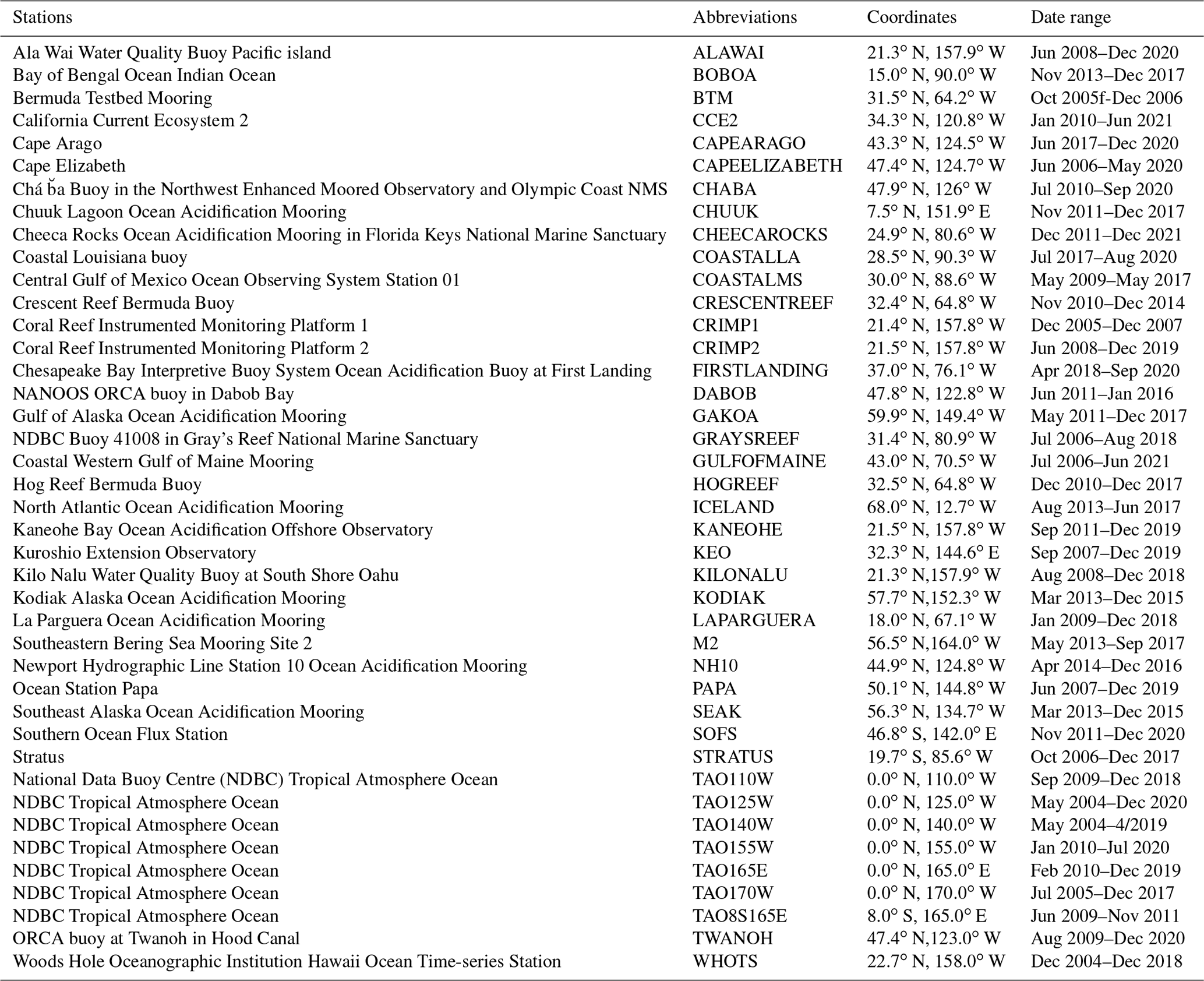
Table A3Statistics computed between CMEMS-LSCE datasets (0.25∘) and time series of pCO2 and pH measurements (Sutton et al., 2019) at open-ocean (O) and coastal stations (C): total numbers of monthly mean observations (N), temporal standard deviation of observations from their monthly averages (σt), RMSD (Eq. 10), and r2 (Eq. 11). See Table A2 and Fig. A1b for stations' information and locations.
Table A4Statistics computed between CMEMS-LSCE datasets (0.25∘) and time series of AT and CT measurements (0–10 m depth): total numbers of monthly mean observations (N), temporal standard deviation of observations from their monthly averages (σt), RMSD (Eq. 10), and r2 (Eq. 11). See Table 2 and Fig. A1b for stations' information and locations.
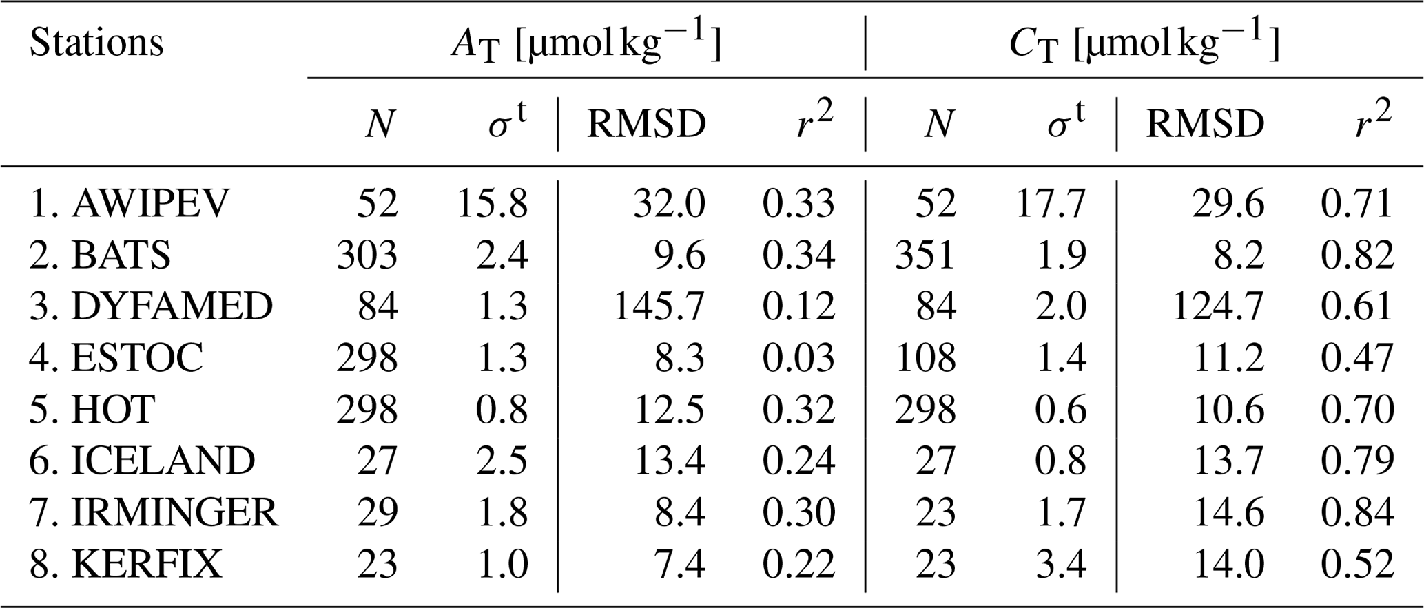
TTTC, FC, and MG developed the CMEMS-LSCE-FFNN model at a quarter-degree resolution. TTTC has prepared script codes and executed the experiments with support from FC in setting and running the model with the HPC resources of TGCC. TTTC, MG, NM, and FC shaped the first paper version. All the authors contributed to the paper revision.
The contact author has declared that none of the authors has any competing interests.
Publisher's note: Copernicus Publications remains neutral with regard to jurisdictional claims made in the text, published maps, institutional affiliations, or any other geographical representation in this paper. While Copernicus Publications makes every effort to include appropriate place names, the final responsibility lies with the authors.
This research was granted access to the HPC resources of TGCC under the allocation no. A0110102201 made by GENCI. The Surface Ocean CO2 Atlas (SOCAT, http://www.socat.info, last access: 20 March 2023) is an international effort endorsed by the International Ocean Carbon Coordination Project (IOCCP), the Surface Ocean Lower Atmosphere Study (SOLAS), and the Integrated Marine Biogeochemistry and Ecosystem Research programme (IMBER) to deliver a uniformly quality-controlled surface ocean CO2 database. The Global Ocean Data Analysis Project (GLODAP, http://www.glodap.info, last access: 21 August 2023) provides access to ocean surface-to-bottom quality-controlled data of carbonate system variables collected through international cruises. We thank Anna Conchon for her help in testing and wrapping LIAR and CO2SYS MATLAB toolboxes. We are grateful for the constructive comments from the editor and two anonymous reviewers, which helped refine the paper.
This research has been supported by the European Copernicus Marine Environment Monitoring Service (CMEMS) (https://marine.copernicus.eu/about/producers/mob-tac, last access: 14 March 2023) (grant no. 83-CMEMSTAC-MOB).
This paper was edited by Anton Velo and reviewed by two anonymous referees.
Bakker, D., Alin, S., Becker, M., Bittig, H., Castaño-Primo, R., Feely, R. A., Gritzalis, T., Kadono, K., Kozyr, A., Lauvset, S. K., Metzl, N., Munro, D., Nakaoka, S.-i., Nojiri, Y., O'Brien, K., Olsen, A., Pfeil, B., Pierrot, D., Steinhoff, T., Sullivan, K., Sutton, A., Sweeney, C., Tilbrook, B., Wada13, C., Wanninkhof, R., Wranne, A. W., et al.: SOCAT version 2022 for quantification of ocean CO2 uptake, https://www.socat.info/wp-content/uploads/2022/06/2022_Poster_SOCATv2022_release.pdf (last access: 17 June 2022), 2022. a, b, c, d
Bakker, D. C. E., Pfeil, B., Landa, C. S., Metzl, N., O'Brien, K. M., Olsen, A., Smith, K., Cosca, C., Harasawa, S., Jones, S. D., Nakaoka, S., Nojiri, Y., Schuster, U., Steinhoff, T., Sweeney, C., Takahashi, T., Tilbrook, B., Wada, C., Wanninkhof, R., Alin, S. R., Balestrini, C. F., Barbero, L., Bates, N. R., Bianchi, A. A., Bonou, F., Boutin, J., Bozec, Y., Burger, E. F., Cai, W.-J., Castle, R. D., Chen, L., Chierici, M., Currie, K., Evans, W., Featherstone, C., Feely, R. A., Fransson, A., Goyet, C., Greenwood, N., Gregor, L., Hankin, S., Hardman-Mountford, N. J., Harlay, J., Hauck, J., Hoppema, M., Humphreys, M. P., Hunt, C. W., Huss, B., Ibánhez, J. S. P., Johannessen, T., Keeling, R., Kitidis, V., Körtzinger, A., Kozyr, A., Krasakopoulou, E., Kuwata, A., Landschützer, P., Lauvset, S. K., Lefèvre, N., Lo Monaco, C., Manke, A., Mathis, J. T., Merlivat, L., Millero, F. J., Monteiro, P. M. S., Munro, D. R., Murata, A., Newberger, T., Omar, A. M., Ono, T., Paterson, K., Pearce, D., Pierrot, D., Robbins, L. L., Saito, S., Salisbury, J., Schlitzer, R., Schneider, B., Schweitzer, R., Sieger, R., Skjelvan, I., Sullivan, K. F., Sutherland, S. C., Sutton, A. J., Tadokoro, K., Telszewski, M., Tuma, M., van Heuven, S. M. A. C., Vandemark, D., Ward, B., Watson, A. J., and Xu, S.: A multi-decade record of high-quality fCO2 data in version 3 of the Surface Ocean CO2 Atlas (SOCAT), Earth Syst. Sci. Data, 8, 383–413, https://doi.org/10.5194/essd-8-383-2016, 2016. a, b, c, d, e, f, g
Bates, N. R., Astor, Y. M., Church, M. J., Currie, K., Dore, J. E., González-Dávila, M., Lorenzoni, L., Muller-Karger, F., Olafsson, J., and Santana-Casiano, J. M.: A time-series view of changing surface ocean chemistry due to ocean uptake of anthropogenic CO2 and ocean acidification, Oceanography, 27, 126–141, 2014. a, b, c, d, e, f, g, h, i, j, k, l, m, n, o, p, q, r
Bresnahan, P. J., Takeshita, Y., Wirth, T., Martz, T. R., Cyronak, T., Albright, R., Wolfe, K., Warren, J. K., and Mertz, K.: Autonomous in situ calibration of ion-sensitive field effect transistor pH sensors, Limnol. Oceanogr.-Meth., 19, 132–144, 2021. a
Broullón, D., Pérez, F. F., Velo, A., Hoppema, M., Olsen, A., Takahashi, T., Key, R. M., Tanhua, T., González-Dávila, M., Jeansson, E., Kozyr, A., and van Heuven, S. M. A. C.: A global monthly climatology of total alkalinity: a neural network approach, Earth Syst. Sci. Data, 11, 1109–1127, https://doi.org/10.5194/essd-11-1109-2019, 2019. a, b
Canadell, J. G., Monteiro, P. M. S., Costa, M. H., Cotrim da Cunha, L., Cox, P. M., Eliseev, A. V., Henson, S., Ishii, M., Jaccard, S., Koven, C., Lohila, A., Patra, P. K., Piao, S., Rogelj, J., Syampungani, S., Zaehle, S., and Zickfeld, K.: Global carbon and other biogeochemical cycles and feedbacks, in: Climate Change 2021: The Physical Science Basis. Contribution of Working Group I to the Sixth Assessment Report of the Intergovernmental Panel on Climate Change, Cambridge University Press, https://doi.org/10.1017/9781009157896.007, 2021. a
Carter, B. R., Williams, N. L., Gray, A. R., and Feely, R. A.: Locally interpolated alkalinity regression for global alkalinity estimation, Limnol. Oceanogr.-Meth., 14, 268–277, https://doi.org/10.1002/lom3.10087, 2016. a, b, c, d
Carter, B. R., Feely, R. A., Williams, N. L., Dickson, A. G., Fong, M. B., and Takeshita, Y.: Updated methods for global locally interpolated estimation of alkalinity, pH, and nitrate, Limnol. Oceanogr.-Meth., 16, 119–131, https://doi.org/10.1002/lom3.10232, 2018. a, b, c, d, e, f, g
Chau, T. T. T., Gehlen, M., and Chevallier, F.: Global ocean surface carbon product, Research Report CMEMS-MOB-QUID-015-008, Le Laboratoire des Sciences du Climat et de l'Environnement, https://doi.org/10.48670/moi-00047, quality Information Document, 2022a. a, b
Chau, T. T. T., Gehlen, M., and Chevallier, F.: A seamless ensemble-based reconstruction of surface ocean pCO2 and air–sea CO2 fluxes over the global coastal and open oceans, Biogeosciences, 19, 1087–1109, https://doi.org/10.5194/bg-19-1087-2022, 2022b. a, b, c, d, e, f, g, h, i, j, k, l, m, n
Chau, T. T. T., Gehlen, M., Metzl, N., and Chevallier, F.: CMEMS-LSCE: A global 0.25-degree, monthly reconstruction of the surface ocean carbonate system, ESPRI/IPSL [dataset], https://doi.org/10.14768/a2f0891b-763a-49e9-af1b-78ed78b16982, 2023. a
Chevallier, F.: On the parallelization of atmospheric inversions of CO2 surface fluxes within a variational framework, Geosci. Model Dev., 6, 783–790, https://doi.org/10.5194/gmd-6-783-2013, 2013. a, b
Chevallier, F., Fisher, M., Peylin, P., Serrar, S., Bousquet, P., Bréon, F.-M., Chédin, A., and Ciais, P.: Inferring CO2 sources and sinks from satellite observations: Method and application to TOVS data, J. Geophys. Res.-Atmos., 110, D24309, https://doi.org/10.1029/2005JD006390, 2005. a, b
Chevallier, F., Ciais, P., Conway, T. J., Aalto, T., Anderson, B. E., Bousquet, P., Brunke, E. G., Ciattaglia, L., Esaki, Y., Fröhlich, M., Gomez, A., Gomez-Pelaez, A. J., Haszpra, L., Krummel, P. B., Langenfelds, R. L., Leuenberger, M., Machida, T., Maignan, F., Matsueda, H., Morguí, J. A., Mukai, H., Nakazawa, T., Peylin, P., Ramonet, M., Rivier, L., Sawa, Y., Schmidt, M., Steele, L. P., Vay, S. A., Vermeulen, A. T., Wofsy, S., and Worthy, D.: CO2 surface fluxes at grid point scale estimated from a global 21 year reanalysis of atmospheric measurements, J. Geophys. Res.-Atmos., 115, D21307, https://doi.org/10.1029/2010JD013887, 2010. a, b
Coppola, L., Boutin, J., Gattuso, J.-P., Lefevre, D., and Metzl, N.: The Carbonate System in the Ligurian Sea, chap. 4, pp. 79–103, John Wiley & Sons, Ltd, https://doi.org/10.1002/9781119706960.ch4, 2020. a, b, c
Coppola, L., Diamond, R. E., and Carval, T.: Dyfamed observatory data, SEANOE [dataset], https://doi.org/10.17882/43749, 2021. a, b, c
Denvil-Sommer, A., Gehlen, M., Vrac, M., and Mejia, C.: LSCE-FFNN-v1: a two-step neural network model for the reconstruction of surface ocean pCO2 over the global ocean, Geosci. Model Dev., 12, 2091–2105, https://doi.org/10.5194/gmd-12-2091-2019, 2019. a
Dickson, A. G.: Standard potential of the reaction: AgCl(s) + 12 H2(g) = Ag(s) + HCl(aq) and the standard acidity constant of the ion in synthetic sea-water from 273.15 K to 318.15 K, J. Chem. Thermodyn., 22, 113–127, https://doi.org/10.1016/0021-9614(90)90074-z, 1990. a
Dickson, A. G.: The carbon dioxide system in seawater: equilibrium chemistry and measurements in Guide to best practices for ocean acidification research and data reporting, https://www.pmel.noaa.gov/co2/files/dickson_thecarbondioxidesysteminseawater_equilibriumchemistryandmeasurementspp17-40.pdf (last access: 12 August 2023), 2010. a, b
Dickson, A. G., Sabine, C. L., and Christian, J. R.: Guide to best practices for ocean CO2 measurement, Sidney, British Columbia, North Pacific Marine Science Organization, 191 pp., PICES Special Publication 3, IOCCP Report 8, https://doi.org/10.25607/OBP-1342, 2007. a, b, c, d
Doney, S. C., Fabry, V. J., Feely, R. A., and Kleypas, J. A.: Ocean acidification: the other CO2 problem, Annu. Rev. Mar. Sci., 1, 169–192, 2009. a
Doney, S. C., Busch, D. S., Cooley, S. R., and Kroeker, K. J.: The impacts of ocean acidification on marine ecosystems and reliant human communities, Annu. Rev. Env. Resour., 45, 83–112, https://doi.org/10.1146/annurev-environ-012320-083019, 2020. a
Dore, J. E., Lukas, R., Sadler, D. W., Church, M. J., and Karl, D. M.: Physical and biogeochemical modulation of ocean acidification in the central North Pacific, P. Natl. Acad. Sci. USA, 106, 12235–12240, 2009. a, b, c, d, e
Droghei, R., Buongiorno Nardelli, B., and Santoleri, R.: A new global sea surface salinity and density dataset from multivariate observations (1993–2016), Frontiers in Marine Science, 5, https://doi.org/10.3389/fmars.2018.00084, 2018. a, b
Fabry, V. J., Seibel, B. A., Feely, R. A., and Orr, J. C.: Impacts of ocean acidification on marine fauna and ecosystem processes, ICES J. Mar. Sci., 65, 414–432, 2008. a
Feely, R. A., Wanninkhof, R., Takahashi, T., and Tans, P.: Influence of El Niño on the equatorial Pacific contribution to atmospheric CO2 accumulation, Nature, 398, 597–601, 1999. a
Feely, R. A., Sabine, C. L., Takahashi, T., and Wanninkhof, R.: Uptake And Storage Of Carbon Dioxide In The Ocean: The Global CO2 Survey, The Oceanography Society, Washington, DC, Oceanography, 14, 18–32, 2001. a
Fischer, P., Schwanitz, M., Loth, R., Posner, U., Brand, M., and Schröder, F.: First year of practical experiences of the new Arctic AWIPEV-COSYNA cabled Underwater Observatory in Kongsfjorden, Spitsbergen, Ocean Sci., 13, 259–272, https://doi.org/10.5194/os-13-259-2017, 2017. a, b
Friedlingstein, P., O'Sullivan, M., Jones, M. W., Andrew, R. M., Gregor, L., Hauck, J., Le Quéré, C., Luijkx, I. T., Olsen, A., Peters, G. P., Peters, W., Pongratz, J., Schwingshackl, C., Sitch, S., Canadell, J. G., Ciais, P., Jackson, R. B., Alin, S. R., Alkama, R., Arneth, A., Arora, V. K., Bates, N. R., Becker, M., Bellouin, N., Bittig, H. C., Bopp, L., Chevallier, F., Chini, L. P., Cronin, M., Evans, W., Falk, S., Feely, R. A., Gasser, T., Gehlen, M., Gkritzalis, T., Gloege, L., Grassi, G., Gruber, N., Gürses, Ö., Harris, I., Hefner, M., Houghton, R. A., Hurtt, G. C., Iida, Y., Ilyina, T., Jain, A. K., Jersild, A., Kadono, K., Kato, E., Kennedy, D., Klein Goldewijk, K., Knauer, J., Korsbakken, J. I., Landschützer, P., Lefèvre, N., Lindsay, K., Liu, J., Liu, Z., Marland, G., Mayot, N., McGrath, M. J., Metzl, N., Monacci, N. M., Munro, D. R., Nakaoka, S.-I., Niwa, Y., O'Brien, K., Ono, T., Palmer, P. I., Pan, N., Pierrot, D., Pocock, K., Poulter, B., Resplandy, L., Robertson, E., Rödenbeck, C., Rodriguez, C., Rosan, T. M., Schwinger, J., Séférian, R., Shutler, J. D., Skjelvan, I., Steinhoff, T., Sun, Q., Sutton, A. J., Sweeney, C., Takao, S., Tanhua, T., Tans, P. P., Tian, X., Tian, H., Tilbrook, B., Tsujino, H., Tubiello, F., van der Werf, G. R., Walker, A. P., Wanninkhof, R., Whitehead, C., Willstrand Wranne, A., Wright, R., Yuan, W., Yue, C., Yue, X., Zaehle, S., Zeng, J., and Zheng, B.: Global Carbon Budget 2022, Earth Syst. Sci. Data, 14, 4811–4900, https://doi.org/10.5194/essd-14-4811-2022, 2022. a, b
Garcia, H. E., Weathers, K. W., Paver, C. R., Smolyar, I., Boyer, T. P., Locarnini, R. A., Zweng, M. M., Mishonov, A. V., Baranova, O. K., Seidov, D., and Reagan, J. R.: World Ocean Atlas 2018. Vol. 4: Dissolved Inorganic Nutrients (phosphate, nitrate and nitrate+nitrite, silicate). A. Mishonov Technical Editor, NOAA Atlas NESDIS 84, 35 pp., https://archimer.ifremer.fr/doc/00651/76336/ (last access: 30 July 2022), 2019. a, b, c
Gattuso, J.-P. and Hansson, L.: Ocean acidification, Oxford University Press, ISBN 978-0-19-959108, 2011. a
Gattuso, J.-P., Alliouane, S., and Fischer, P.: High-frequency, year-round time series of the carbonate chemistry in a high-Arctic fjord (Svalbard), Earth Syst. Sci. Data, 15, 2809–2825, https://doi.org/10.5194/essd-15-2809-2023, 2023a. a, b
Gattuso, J.-P., Alliouane, S., and Fischer, P.: High-frequency, year-round time series of the carbonate chemistry in a high-Arctic fjord (Svalbard) v2, PANGAEA [data set], https://doi.org/10.1594/PANGAEA.960131, 2023b. a
Gehlen, M., Gruber, N., Gangstø, R., Bopp, L., and Oschlies, A.: Biogeochemical consequences of ocean acidification and feedbacks to the earth system, in: Ocean acidification, edited by: Gattuso J.-P. and Hansson L., 1, 230–248, https://doi.org/10.1093/oso/9780199591091.003.0017, 2011. a
González-Dávila, M. and Santana-Casiano, J.: Sea surface and atmospheric fCO2 data measured during the estoc time series cruises from 1995–2009, CDIAC, Oak Ridge National Laboratory, US Department of Energy, Oak Ridge, Tennessee, 10, 2009. a, b, c, d, e
Good, S.: Global Ocean OSTIA Sea Surface Temperature and Sea Ice Analysis, E.U Copernicus Marine Service Information (CMEMS), Marine Data Store (MDS) [data set], https://doi.org/10.48670/moi-00165, 2022. a
Good, S. and Worsfold, M.: Global Ocean OSTIA Sea Surface Temperature and Sea Ice Reprocessed, E.U Copernicus Marine Service Information (CMEMS), Marine Data Store (MDS) [data set], https://doi.org/10.48670/moi-00168, 2022. a
Good, S., Fiedler, E., Mao, C., Martin, M. J., Maycock, A., Reid, R., Roberts-Jones, J., Searle, T., Waters, J., While, J., and Worsfold, M.: The Current Configuration of the OSTIA System for Operational Production of Foundation Sea Surface Temperature and Ice Concentration Analyses, Remote Sens.-Basel, 12, 720, https://doi.org/10.3390/rs12040720, 2020. a
Gregor, L. and Gruber, N.: OceanSODA-ETHZ: a global gridded data set of the surface ocean carbonate system for seasonal to decadal studies of ocean acidification, Earth Syst. Sci. Data, 13, 777–808, https://doi.org/10.5194/essd-13-777-2021, 2021. a, b, c, d, e, f, g, h, i, j
Gregor, L., Lebehot, A. D., Kok, S., and Scheel Monteiro, P. M.: A comparative assessment of the uncertainties of global surface ocean CO2 estimates using a machine-learning ensemble (CSIR-ML6 version 2019a) – have we hit the wall?, Geosci. Model Dev., 12, 5113–5136, https://doi.org/10.5194/gmd-12-5113-2019, 2019. a, b
Gruber, N., Clement, D., Carter, B. R., Feely, R. A., Van Heuven, S., Hoppema, M., Ishii, M., Key, R. M., Kozyr, A., Lauvset, S. K., and Lo Monaco, C.: The oceanic sink for anthropogenic CO2 from 1994 to 2007, Science, 363, 1193–1199, 2019. a
Hauck, J., Zeising, M., Le Quéré, C., Gruber, N., Bakker, D. C., Bopp, L., Chau, T. T. T., Gürses, Ö., Ilyina, T., Landschützer, P., Lenton, A., Resplandy, L., Rödenbeck, C., Schwinger, J., and Séférian, R.: Consistency and Challenges in the Ocean Carbon Sink Estimate for the Global Carbon Budget, Frontiers in Marine Science, 7, 852, https://doi.org/10.3389/fmars.2020.571720, 2020. a
Hoffmann, L. J., Breitbarth, E., Boyd, P. W., and Hunter, K. A.: Influence of ocean warming and acidification on trace metal biogeochemistry, Mar. Ecol. Prog. Ser., 470, 191–205, 2012. a
Hopkins, F. E., Suntharalingam, P., Gehlen, M., Andrews, O., Archer, S. D., Bopp, L., Buitenhuis, E., Dadou, I., Duce, R., Goris, N., Jickells, T., , Johnson M., Keng F., Law C. S., Lee K., Liss P. S., Lizotte M., Malin G., Murrell J. C., Naik H., Rees A. P., Schwinger J., and Williamson P.: The impacts of ocean acidification on marine trace gases and the implications for atmospheric chemistry and climate, P. Roy. Soc. A, 476, 20190769, https://doi.org/10.1098/rspa.2019.0769, 2020. a, b
Ibánhez, J. S. P., Diverrès, D., Araujo, M., and Lefèvre, N.: Seasonal and interannual variability of sea-air CO2 fluxes in the tropical Atlantic affected by the Amazon River plume, Global Biogeochem. Cy., 29, 1640–1655, 2015. a
Iida, Y., Takatani, Y., Kojima, A., and Ishii, M.: Global trends of ocean CO2 sink and ocean acidification: an observation-based reconstruction of surface ocean inorganic carbon variables, J. Oceanogr., 77, 323–358, 2021. a, b, c, d
Jiang, L.-Q., Carter, B. R., Feely, R. A., Lauvset, S. K., and Olsen, A.: Surface ocean pH and buffer capacity: past, present and future, Sci. Rep.-UK, 9, 1–11, 2019. a, b
Jones, S., Le Quéré, C., and Rödenbeck, C.: Autocorrelation characteristics of surface ocean pCO2 and air–sea CO2 fluxes, Global Biogeochem. Cy., 26, GB2042, https://doi.org/10.1029/2010GB004017, 2012. a, b
Key, R. M., Kozyr, A., Sabine, C. L., Lee, K., Wanninkhof, R., Bullister, J. L., Feely, R. A., Millero, F. J., Mordy, C., and Peng, T.-H.: A global ocean carbon climatology: Results from Global Data Analysis Project (GLODAP), Global Biogeochem. Cy., 18, GB4031, https://doi.org/10.1029/2004GB002247, 2004. a
Körtzinger, A.: Determination of carbon dioxide partial pressure (pCO2), chap. 9, John Wiley & Sons, Ltd, 149–158, https://doi.org/10.1002/9783527613984.ch9, 1999. a, b
Landschützer, P., Gruber, N., and Bakker, D. C.: Decadal variations and trends of the global ocean carbon sink, Global Biogeochem. Cy., 30, 1396–1417, 2016. a, b, c, d
Landschützer, P., Ilyina, T., and Lovenduski, N. S.: Detecting Regional Modes of Variability in Observation-Based Surface Ocean pCO2, Geophys. Res. Lett., 46, 2670–2679, 2019. a
Landschützer, P., Laruelle, G. G., Roobaert, A., and Regnier, P.: A uniform pCO2 climatology combining open and coastal oceans, Earth Syst. Sci. Data, 12, 2537–2553, https://doi.org/10.5194/essd-12-2537-2020, 2020. a, b
Laruelle, G. G., Landschützer, P., Gruber, N., Tison, J.-L., Delille, B., and Regnier, P.: Global high-resolution monthly pCO2 climatology for the coastal ocean derived from neural network interpolation, Biogeosciences, 14, 4545–4561, https://doi.org/10.5194/bg-14-4545-2017, 2017. a, b
Lauvset, S. K. and Gruber, N.: Long-term trends in surface ocean pH in the North Atlantic, Mar. Chem., 162, 71–76, 2014. a
Lauvset, S. K., Gruber, N., Landschützer, P., Olsen, A., and Tjiputra, J.: Trends and drivers in global surface ocean pH over the past 3 decades, Biogeosciences, 12, 1285–1298, https://doi.org/10.5194/bg-12-1285-2015, 2015. a, b, c, d
Lauvset, S. K., Lange, N., Tanhua, T., Bittig, H. C., Olsen, A., Kozyr, A., Alin, S., Álvarez, M., Azetsu-Scott, K., Barbero, L., Becker, S., Brown, P. J., Carter, B. R., da Cunha, L. C., Feely, R. A., Hoppema, M., Humphreys, M. P., Ishii, M., Jeansson, E., Jiang, L.-Q., Jones, S. D., Lo Monaco, C., Murata, A., Müller, J. D., Pérez, F. F., Pfeil, B., Schirnick, C., Steinfeldt, R., Suzuki, T., Tilbrook, B., Ulfsbo, A., Velo, A., Woosley, R. J., and Key, R. M.: GLODAPv2.2022: the latest version of the global interior ocean biogeochemical data product, Earth Syst. Sci. Data, 14, 5543–5572, https://doi.org/10.5194/essd-14-5543-2022, 2022a. a, b, c, d, e, f
Lauvset, S. K., Lange, N., Tanhua, T., Bittig, H. C., Olsen, A., Kozyr, A., Alin, S., Álvarez, M., Azetsu-Scott, K., Barbero, L., Becker, S., Brown, P. J., Carter, B. R., da Cunha, L. C., Feely, R. A., Hoppema, M., Humphreys, M. P., Ishii, M., Jeansson, E., Jiang, L.-Q., Jones, S. D., Lo Monaco, C., Murata, A., Müller, J. D., Pérez, F. F., Pfeil, B., Schirnick, C., Steinfeldt, R., Suzuki, T., Tilbrook, B., Ulfsbo, A., Velo, A., Woosley, R. J., and Key, R. M.: Global Ocean Data Analysis Project version 2.2022 (GLODAPv2.2022) (NCEI Accession 0257247), NOAA National Centers for Environmental Information [dataset], https://doi.org/10.25921/1f4w-0t92, 2022b. a, b, c
Lee, K., Tong, L. T., Millero, F. J., Sabine, C. L., Dickson, A. G., Goyet, C., Park, G.-H., Wanninkhof, R., Feely, R. A., and Key, R. M.: Global relationships of total alkalinity with salinity and temperature in surface waters of the world's oceans, Geophys. Res. Lett. 33, L19605, https://doi.org/10.1029/2006GL027207, 2006. a
Leseurre, C., Lo Monaco, C., Reverdin, G., Metzl, N., Fin, J., Mignon, C., and Benito, L.: Summer trends and drivers of sea surface fCO2 and pH changes observed in the southern Indian Ocean over the last two decades (1998–2019), Biogeosciences, 19, 2599–2625, https://doi.org/10.5194/bg-19-2599-2022, 2022. a, b, c
Lewis, E. and Wallace, D.: CO2SYS-Program developed for the CO2 system calculations, Carbon Dioxide Inf Anal Center Report ORNL/CDIAC-105, Oak Ridge National Laboratory, US Department of Energy, Oak Ridge, TN, USA, https://doi.org/10.15485/1464255, 1998. a, b, c, d
Lueker, T. J., Dickson, A. G., and Keeling, C. D.: Ocean pCO2 calculated from dissolved inorganic carbon, alkalinity, and equations for K1 and K2: validation based on laboratory measurements of CO2 in gas and seawater at equilibrium, Mar. Chem., 70, 105–119, 2000. a
Ma, D., Gregor, L., and Gruber, N.: Four Decades of Trends and Drivers of Global Surface Ocean Acidification, Global Biogeochem. Cy., 37, e2023GB007765, https://doi.org/10.1029/2023GB007765, 2023. a, b
Maritorena, S., d'Andon, O. H. F., Mangin, A., and Siegel, D. A.: Merged satellite ocean color data products using a bio-optical model: Characteristics, benefits and issues, Remote Sens. Environ., 114, 1791–1804, https://doi.org/10.1016/j.rse.2010.04.002, 2010. a, b
Menemenlis, D., Campin, J., Heimbach, P., Hill, C., Lee, T., Nguyen, A., Schodlok, M., and Zhang, H.: ECCO2: High Resolution Global Ocean and Sea Ice Data Synthesis, 2008, OS31C-1292, 2008. a, b
Menviel, L., Spence, P., Yu, J., Chamberlain, M., Matear, R., Meissner, K., and England, M. H.: Southern Hemisphere westerlies as a driver of the early deglacial atmospheric CO2 rise, Nat. Commun., 9, 1–12, 2018. a
Metzl, N. and Lo Monaco, C.: OISO – Ocean Indien Service d'Observation, Campagnes Océanographiques Françaises [data set], https://doi.org/10.18142/228, 1998. a, b, c
Michaels, A. F. and Knap, A. H.: Overview of the US JGOFS Bermuda Atlantic Time-series Study and the Hydrostation S program, Deep-Sea Res. Pt. II, 43, 157–198, 1996. a, b
Millero, F. J., Woosley, R., Ditrolio, B., and Waters, J.: Effect of ocean acidification on the speciation of metals in seawater, Oceanography, 22, 72–85, 2009. a
Mucci, A.: The solubility of calcite and aragonite in seawater at various salinities, temperatures, and one atmosphere total pressure, Am. J Sci., 283, 780–799, 1983. a
Nardelli, B. B., Droghei, R., and Santoleri, R.: Multi-dimensional interpolation of SMOS sea surface salinity with surface temperature and in situ salinity data, Remote Sens. Environ., 180, 392–402, 2016. a, b
Olafsson, J., Olafsdottir, S. R., Benoit-Cattin, A., and Takahashi, T.: The Irminger Sea and the Iceland Sea time series measurements of sea water carbon and nutrient chemistry 1983–2008, Earth Syst. Sci. Data, 2, 99–104, https://doi.org/10.5194/essd-2-99-2010, 2010. a, b, c
Olivier, L., Boutin, J., Reverdin, G., Lefèvre, N., Landschützer, P., Speich, S., Karstensen, J., Labaste, M., Noisel, C., Ritschel, M., Steinhoff, T., and Wanninkhof, R.: Wintertime process study of the North Brazil Current rings reveals the region as a larger sink for CO2 than expected, Biogeosciences, 19, 2969–2988, https://doi.org/10.5194/bg-19-2969-2022, 2022. a
Olsen, A., Key, R. M., van Heuven, S., Lauvset, S. K., Velo, A., Lin, X., Schirnick, C., Kozyr, A., Tanhua, T., Hoppema, M., Jutterström, S., Steinfeldt, R., Jeansson, E., Ishii, M., Pérez, F. F., and Suzuki, T.: The Global Ocean Data Analysis Project version 2 (GLODAPv2) – an internally consistent data product for the world ocean, Earth Syst. Sci. Data, 8, 297–323, https://doi.org/10.5194/essd-8-297-2016, 2016. a, b, c, d, e
Orr, J. C., Fabry, V. J., Aumont, O., Bopp, L., Doney, S. C., Feely, R. A., Gnanadesikan, A., Gruber, N., Ishida, A., Joos, F., and Key, R. M.: Anthropogenic ocean acidification over the twenty-first century and its impact on calcifying organisms, Nature, 437, 681–686, 2005. a
Orr, J. C., Epitalon, J.-M., Dickson, A. G., and Gattuso, J.-P.: Routine uncertainty propagation for the marine carbon dioxide system, Mar. Chem., 207, 84–107, https://doi.org/10.1016/j.marchem.2018.10.006, 2018. a, b, c, d, e, f
Palmiéri, J., Orr, J. C., Dutay, J.-C., Béranger, K., Schneider, A., Beuvier, J., and Somot, S.: Simulated anthropogenic CO2 storage and acidification of the Mediterranean Sea, Biogeosciences, 12, 781–802, https://doi.org/10.5194/bg-12-781-2015, 2015. a
Park, P. K.: OCEANIC CO2 SYSTEM: AN EVALUATION OF TEN METHODS OF INVESTIGATION1, Limnol. Oceanogr., 14, 179–186, https://doi.org/10.4319/lo.1969.14.2.0179, 1969. a
Pérez, F. F., Olafsson, J., Ólafsdóttir, S. R., Fontela, M., and Takahashi, T.: Contrasting drivers and trends of ocean acidification in the subarctic Atlantic, Sci. Rep.-UK, 11, 1–16, 2021. a, b, c, d, e
Pfeil, B., Olsen, A., Bakker, D. C., Hankin, S., Koyuk, H., Kozyr, A., Malczyk, J., Manke, A., Metzl, N., Sabine, C. L., et al.: A uniform, quality–controlled Surface Ocean CO2 Atlas (SOCAT), Earth System Science Data, 5, 125–143, https://doi.org/10.5194/essd-5-125-2013, 2013. a
Rödenbeck, C., Keeling, R. F., Bakker, D. C. E., Metzl, N., Olsen, A., Sabine, C., and Heimann, M.: Global surface-ocean pCO2 and sea–air CO2 flux variability from an observation-driven ocean mixed-layer scheme, Ocean Sci., 9, 193–216, https://doi.org/10.5194/os-9-193-2013, 2013. a
Rose, A.: Vision: human and electronic, Springer Science & Business Media, https://doi.org/10.1007/978-1-4684-2037-1, 2013. a
Sabine, C. L., Key, R. M., Feely, R. A., and Greeley, D.: Inorganic carbon in the Indian Ocean: Distribution and dissolution processes, Global Biogeochem. Cy., 16, 15–1, 2002. a
Sabine, C. L., Hankin, S., Koyuk, H., Bakker, D. C. E., Pfeil, B., Olsen, A., Metzl, N., Kozyr, A., Fassbender, A., Manke, A., Malczyk, J., Akl, J., Alin, S. R., Bellerby, R. G. J., Borges, A., Boutin, J., Brown, P. J., Cai, W.-J., Chavez, F. P., Chen, A., Cosca, C., Feely, R. A., González-Dávila, M., Goyet, C., Hardman-Mountford, N., Heinze, C., Hoppema, M., Hunt, C. W., Hydes, D., Ishii, M., Johannessen, T., Key, R. M., Körtzinger, A., Landschützer, P., Lauvset, S. K., Lefèvre, N., Lenton, A., Lourantou, A., Merlivat, L., Midorikawa, T., Mintrop, L., Miyazaki, C., Murata, A., Nakadate, A., Nakano, Y., Nakaoka, S., Nojiri, Y., Omar, A. M., Padin, X. A., Park, G.-H., Paterson, K., Perez, F. F., Pierrot, D., Poisson, A., Ríos, A. F., Salisbury, J., Santana-Casiano, J. M., Sarma, V. V. S. S., Schlitzer, R., Schneider, B., Schuster, U., Sieger, R., Skjelvan, I., Steinhoff, T., Suzuki, T., Takahashi, T., Tedesco, K., Telszewski, M., Thomas, H., Tilbrook, B., Vandemark, D., Veness, T., Watson, A. J., Weiss, R., Wong, C. S., and Yoshikawa-Inoue, H.: Surface Ocean CO2 Atlas (SOCAT) gridded data products, Earth Syst. Sci. Data, 5, 145–153, https://doi.org/10.5194/essd-5-145-2013, 2013. a
Sarma, V. V. S. S., Lenton, A., Law, R. M., Metzl, N., Patra, P. K., Doney, S., Lima, I. D., Dlugokencky, E., Ramonet, M., and Valsala, V.: Sea–air CO2 fluxes in the Indian Ocean between 1990 and 2009, Biogeosciences, 10, 7035–7052, https://doi.org/10.5194/bg-10-7035-2013, 2013. a
Sarma, V. V. S. S., Sridevi, B., Metzl, N., Patra, P. K., Lachkar, Z., Chakraborty, K., Goyet, C., Levy, M., Mehari, M., and Chandra, N.: Air-Sea Fluxes of CO2 in the Indian Ocean Between 1985 and 2018: A Synthesis Based on Observation-Based Surface CO2, Hindcast and Atmospheric Inversion Models, Global Biogeochem. Cy., 37, e2023GB007694, https://doi.org/10.1029/2023GB007694, 2023. a
Skjelvan, I., Lauvset, S. K., Johannessen, T., Gundersen, K., and Skagseth, Ø.: Decadal trends in ocean acidification from the Ocean Weather Station M in the Norwegian Sea, J. Marine Syst., 234, 103775, https://doi.org/10.1016/j.jmarsys.2022.103775, 2022. a
Steinberg, D. K., Carlson, C. A., Bates, N. R., Johnson, R. J., Michaels, A. F., and Knap, A. H.: Overview of the US JGOFS Bermuda Atlantic Time-series Study (BATS): a decade-scale look at ocean biology and biogeochemistry, Deep-Sea Res. Pt. II, 48, 1405–1447, 2001. a, b, c
Sutton, A. J., Feely, R. A., Maenner-Jones, S., Musielwicz, S., Osborne, J., Dietrich, C., Monacci, N., Cross, J., Bott, R., Kozyr, A., Andersson, A. J., Bates, N. R., Cai, W.-J., Cronin, M. F., De Carlo, E. H., Hales, B., Howden, S. D., Lee, C. M., Manzello, D. P., McPhaden, M. J., Meléndez, M., Mickett, J. B., Newton, J. A., Noakes, S. E., Noh, J. H., Olafsdottir, S. R., Salisbury, J. E., Send, U., Trull, T. W., Vandemark, D. C., and Weller, R. A.: Autonomous seawater pCO2 and pH time series from 40 surface buoys and the emergence of anthropogenic trends, Earth Syst. Sci. Data, 11, 421–439, https://doi.org/10.5194/essd-11-421-2019, 2019. a, b, c, d, e, f, g, h, i, j, k, l
Takahashi, T., Sutherland, S. C., Wanninkhof, R., Sweeney, C., Feely, R. A., Chipman, D. W., Hales, B., Friederich, G., Chavez, F., Sabine, C., Watson, A., Bakker, D. C., Schuster, U., Metzl, N., Yoshikawa-Inoue, H., Ishii, M., Midorikawa, T., Nojiri, Y., Körtzinger, A., Steinhoff, T., Hoppema, M., Olafsson, J., Arnarson, T. S., Tilbrook, B., Johannessen, T., Olsen, A., Bellerby, R., Wong, C., Delille, B., Bates, N., and de Baar, H. J.: Climatological mean and decadal change in surface ocean pCO2, and net sea–air CO2 flux over the global oceans, Deep-Sea Res. Pt. II, 56, 554–577, https://doi.org/10.1016/j.dsr2.2008.12.009, 2009. a, b
Takahashi, T., Sutherland, S. C., Chipman, D. W., Goddard, J. G., Ho, C., Newberger, T., Sweeney, C., and Munro, D.: Climatological distributions of pH, pCO2, total CO2, alkalinity, and CaCO3 saturation in the global surface ocean, and temporal changes at selected locations, Mar. Chem., 164, 95–125, 2014. a, b, c, d
Thomsen, J., Haynert, K., Wegner, K. M., and Melzner, F.: Impact of seawater carbonate chemistry on the calcification of marine bivalves, Biogeosciences, 12, 4209–4220, https://doi.org/10.5194/bg-12-4209-2015, 2015. a
Uppstrom, L.: The boron/chlorinity ratio of deep-sea water from the Pacific Ocean, Deep-Sea Res., 21, 161–162, 1974. a
Van Heuven, S., Pierrot, D., Rae, J., Lewis, E., and Wallace, D.: CO2SYS v 1.1, MATLAB program developed for CO2 system calculations, ORNL/CDIAC-105b, Oak Ridge National Laboratory, Oak Ridge, TN, https://cdiac.ess-dive.lbl.gov/ftp/co2sys/CO2SYS_calc_MATLAB_v1.1/ (last access: 17 June 2022), 2011. a, b, c
Woosley, R. J.: Evaluation of the temperature dependence of dissociation constants for the marine carbon system using pH and certified reference materials, Mar. Chem., 229, 103914, 2021. a
Zeebe, R. E. and Wolf-Gladrow, D.: CO2 in seawater: equilibrium, kinetics, isotopes, 65, Gulf Professional Publishing, ISBN 978-0-444-50579-8, 2001. a