the Creative Commons Attribution 4.0 License.
the Creative Commons Attribution 4.0 License.
 | 27 Feb 2024
Reconstruction of hourly coastal water levels and counterfactuals without sea level rise for impact attribution
Sanne Muis
Sönke Dangendorf
Thomas Wahl
Julius Oelsmann
Stefanie Heinicke
Katja Frieler
Matthias Mengel
Rising seas are a threat to human and natural systems along coastlines. The relation between global warming and sea level rise is established, but the quantification of impacts of historical sea level rise on a global scale is largely absent. To foster such quantification, here we present a reconstruction of historical hourly (1979–2015) and monthly (1900–2015) coastal water levels and a corresponding counterfactual without long-term trends in sea level. The dataset pair allows for impact attribution studies that quantify the contribution of sea level rise to observed changes in coastal systems following the definition of the Intergovernmental Panel on Climate Change (IPCC). Impacts are ultimately caused by water levels that are relative to the local land height, which makes the inclusion of vertical land motion a necessary step. Also, many impacts are driven by sub-daily extreme water levels. To capture these aspects, the factual data combine reconstructed geocentric sea level on a monthly timescale since 1900, vertical land motion since 1900 and hourly storm-tide variations since 1979. The inclusion of observation-based vertical land motion brings the trends of the combined dataset closer to tide gauge records in most cases, but outliers remain. Daily maximum water levels get in closer agreement with tide gauges through the inclusion of intra-annual ocean density variations. The counterfactual data are derived from the factual data through subtraction of the quadratic trend. The dataset is made available openly through the Inter-Sectoral Impact Model Intercomparison Project (ISIMIP) at https://doi.org/10.48364/ISIMIP.749905 (Treu et al., 2023a).
- Article
(3064 KB) - Full-text XML
-
Supplement
(1320 KB) - BibTeX
- EndNote


Sea level rise is a threat to a significant proportion of the world's population, which is concentrated near the sea. Global sea levels rose by 15 to 25 cm from 1901 to 2018 and are expected to rise by a further 28 (lower bound of the SSP-1.9 scenario) to 101 cm (upper bound of the SSP-8.5 scenario) relative to the period 1995–2014 by 2100 (Fox-Kemper et al., 2021). There are still gaps in the understanding of fast Antarctic ice loss, which may lead to sea level rise above the upper bound of the SSP-8.5 scenario. The trend in relative sea level (RSL) rise is stated as a climate impact driver (Ranasinghe et al., 2021) for seven of the eight Representative Key Risks identified in the Working Group II contribution to the sixth assessment report of the Intergovernmental Panel on Climate Change (IPCC, AR6, WGII, Chapter 16; O'Neill et al., 2022a). It contributes in particular as a driver of risks to low-lying coastal socio-ecological systems through irreversible long-term loss of land, critical ecosystem services, livelihoods, wellbeing or culture in combination with other drivers of risk.
Several studies assessed the future coastal risks from sea level rise and incorporated important drivers such as socio-economic development and population change (Hallegatte et al., 2013; Hinkel et al., 2014; Neumann et al., 2015; Hunter et al., 2017; Brown et al., 2018; Tiggeloven et al., 2020; Vousdoukas et al., 2020; Kirezci et al., 2023). There is, however, an absence of works on observed impacts attributed to sea level rise, though similar modeling approaches could be used. In particular, there is a lack of studies to attribute historical coastal change or disturbances to sea level rise in a global setting (O'Neill et al., 2022a).
Studies on a regional scale exist. They attributed changes in the physical quantities of historic flood events, e.g., for Hurricane Katrina (Irish et al., 2014) and Hurricane Sandy (Lin et al., 2016), coastal retreat to sea level rise in Senegal (Enríquez-de-Salamanca, 2020) and Pakistan (Kanwal et al., 2020), abrupt beach retreat in Tasmania to sea level rise and wind changes (Sharples et al., 2020). Strauss et al. (2021) quantified the role of historical sea level rise in economic damages for the individual event of Hurricane Sandy. Observed damages in Solomon Islands and Fiji have been assessed to be driven by relative sea level rise (Albert et al., 2016; McNamara and Des Combes, 2015). These examples are taken from the literature review on impact attribution for the IPCC AR6 WGII Chapter 16 (O'Neill et al., 2022a); see O'Neill et al. (2022b) for a comprehensive overview of studies1.
Challenges for studies on impact attribution to sea level rise include the sparse observational data on flood extent required to validate historical impact simulations on the global scale, with improvements becoming available only recently, e.g., through the Global Flood Database (Tellman et al., 2021) and the Flood Inundation Archive (Yang et al., 2021) for flooded coastal areas. Few datasets exist for longer-term change of coastlines (Mentaschi et al., 2018; Luijendijk et al., 2018). Global digital elevation datasets are another important source of uncertainty as their vertical precision is largely below that of historical sea level change (e.g., Van de Sande et al., 2012; Gesch, 2018), but there are promising recent advances (Hooijer and Vernimmen, 2021; Vernimmen and Hooijer, 2023). There is, however, also a lack of forcing data to facilitate impact attribution to sea level rise.
With this study we aim to address the lack of forcing data and facilitate works that quantify the role of sea level rise in historically observed phenomena at the coast. Such phenomena can be slowly evolving changes like the retreat of sandy beaches or extreme-event-driven effects like economic damages from coastal flooding. Here we build on the impact attribution framework outlined in the IPCC AR6 WG2, ch16 (O'Neill et al., 2022a). The IPCC defines an “observed impact as the difference between the observed state of a natural, human or managed system and a counterfactual baseline that characterizes the system's state in the absence of changes in the climate-related systems” and further that the “difference between the observed and the counterfactual baseline state is considered the change in the natural, human or managed system that is attributed to the changes in the climate-related systems (impact attribution)” (O'Neill et al., 2022a).
As the counterfactual impact baseline cannot be observed, it needs to be modeled by an impact model. A precondition for impact attribution is that the impact model explains the observed phenomenon under consideration reasonably well given its drivers. This necessitates a model evaluation step, which is followed by the attribution step itself. The presented work aims to make forcing data available for both steps: (i) factual forcing data to evaluate impact models and produce factual historical impact simulations and (ii) counterfactual forcing data to produce counterfactual impact simulations.
While the factual data should stay as close as possible to reality and are thus in principle set, the counterfactual data depend on the specific attribution question. As coastal systems changed fast over the past century, with climate and sea level presumably two drivers but often not the dominant ones, here we ask the following attribution question: “how did historical sea level rise affect observed phenomena in dynamic coastal systems with a multitude of drivers, irrespective of the origin of the sea level rise?” We thus aim to delineate sea level rise from other drivers of change like population change, construction activity at the coast or ecosystem degradation through direct human intervention. We do not focus on the causes of sea level rise itself but treat it as one driver of coastal change or disturbance in line with the IPCC definition (O'Neill et al., 2022a). Quantifying the fraction of impacts from anthropogenic influence on sea level rise would need investigation of the causal chain from emissions to sea level rise to impacts through a more complex attribution setup based on climate model ensembles (Hope et al., 2022).
Coastal systems ultimately experience the change of the water level at the coast relative to the height of the land, which we term relative water levels. As relative water levels are the most direct input for impact models, we provide factual and counterfactual relative water levels. This necessitates the inclusion of vertical land motion (VLM), which – though an important driver of coastal impacts – has been less rigorously observed and researched on a global level than sea level, and global datasets have only recently become available (Oelsmann et al., 2024; Hammond et al., 2021; Frederikse et al., 2020; Hawkins et al., 2019b; Pfeffer et al., 2017). Consistent with the impact attribution definition of the IPCC, we do not investigate the drivers of VLM itself but treat it as a driver of impacts as a part of the relative sea level. There is no predecessor for a global relative water level dataset.
We construct relative hourly and extended monthly coastal water levels globally for the historical period and a respective counterfactual – the hourly coastal water levels with counterfactual (HCC) dataset. We describe the approach in the “Materials and methods” section, present the main features of the dataset in the subsequent “Results” section, and provide a discussion in the final section.
Many impacts manifest through extreme sea level conditions that occur on the timescale of hours, which necessitates a product that resolves these timescales. The construction of factual relative hourly coastal water levels in our HCC dataset can be broken down into the sum of four components:
where h is the water level relative to the coast, hLF is a low-frequency component that includes the long-term evolution of water levels and VLM, hHF is a high-frequency component that describes hourly changes in water levels, hT is the tidal component, and hSC is the regular seasonal cycle. We derive them as follows:
-
hLF (low frequency). This was derived from a geocentric, deseasonalized version of the hybrid reconstruction (HR) dataset from Dangendorf et al. (2019) and a probabilistic VLM reconstruction from Oelsmann et al. (2024). This combined dataset is low-pass-filtered by taking its 90 d running mean value to retain only contributions with frequency longer than 3 months. To yield hourly resolution, the result is interpolated with cubic spline interpolation.
-
hHF (high frequency). This was sourced from deseasonalized non-tidal residuals of the Coastal Dataset for the Evaluation of Climate impact (CoDEC; Muis et al., 2020) to cover the high-frequency variation of storm tides. This is then high-pass-filtered by removing the 90 d running mean value, to represent water level frequencies higher than 3 months.
-
hT (tidal levels). This was derived from the tidal component of CoDEC.
-
hSC (seasonal cycle). This denotes the multiyear seasonality computed over the years 1993 to 2015 from the satellite altimetry dataset used in Dangendorf et al. (2019). To yield hourly resolution, the seasonal cycle is interpolated with cubic spline interpolation.
To ensure no overlap, the regular seasonal cycle is excluded from both hLF and hHF components. Barotropic water level changes due to wind and atmospheric pressure on timescales longer than or equal to 1 month are covered in both the HR and the CoDEC dataset. We use frequency filtering to prevent double counting. CoDEC models these water level changes explicitly, whereas HR is based on a statistical reconstruction method based on sparse observations. However, HR is not restricted to barotropic variations alone and covers the full spectrum of intra-annual and longer sea level variations (including sterodynamic and barystatic processes). The dominating process at different timescales depends on local conditions (Zhu et al., 2021; Dangendorf et al., 2014). We thus expect that it depends on the location which product performs better. Our method's cutoff frequency determines which scale of variations is captured by each product. CoDEC captures variations with higher frequencies than the cutoff, while HR captures variations with lower frequencies. We have tested for different cutoff frequencies and how it affects the performance of the combined product when compared to tide gauges. We varied the cutoff frequency for values of 1, 2, 3, 4, 5, 6, and 12 months and found an optimal cutoff frequency of 3 months (90 d).
We apply the same process but exclude the VLM reconstruction to yield a geocentric version of the combined dataset. To yield a common vertical reference, we shift the geocentric version of our dataset vertically to yield instantaneous height above the WGS 84 geoid, which is also called absolute dynamic topography. To that end, we remove the mean value for the time period 1993–2012 from our geocentric dataset and add the mean dynamic topography from Copernicus Marine Environment Monitoring Service (CMEMS) SEALEVEL_GLO_PHY_MDT_008_063 https://doi.org/10.48670/moi-00150 (E.U. Copernicus Marine Service Information (CMEMS), 2024) that is derived from satellite altimetry over the same time period. We align our relative version of the dataset with the geocentric version such that the water levels in both datasets are equal on the last date of the record.
We describe in Sect. 2.1, 2.2 and 2.3 the different source datasets and how we adjusted them for this application. We describe how we derived the counterfactual dataset in Sect. 2.5, “Counterfactual water levels”.
2.1 Coastal Dataset for the Evaluation of Climate impact (CoDEC)
CoDEC is an update of the Global Tide and Surge Reanalysis (GTSR; Muis et al., 2016) dataset and uses a newer modeling framework, with higher-resolution and newer climate forcing data. It is based on the hydrodynamic Global Tide and Surge Model (GTSMv3.0), which uses the unstructured Delft3D Flexible Mesh software (Kernkamp et al., 2011) as the shallow-water flow solver and resolves coastal areas at high detail while being efficiently coarse in the open ocean. GTSM uses the depth-averaged, barotropic mode of Delft3D, assuming a constant density of ocean waters. It explicitly models tides and storm surges at a high temporal resolution. The model has global coverage and thus no open boundaries. The coastal resolution is 1.25 km at European coasts and 2.5 km at other global coasts. To produce CoDEC, GTSM is forced with the 10 m wind speed and atmospheric pressure from the ERA5 reanalysis (Hersbach et al., 2020). ERA5 determines the time coverage of CoDEC from 1979 to 2017. The spatial resolution of ERA5 is 0.25°×0.25° (∼31 km). Time series are saved at approximately 18 000 output locations that are located at 10–50 km distance along a smoothed global coastline. Validation by Muis et al. (2020) has demonstrated that CoDEC has an average root mean squared error (RMSE) of 0.26 m (SD 0.73 m) for the comparison between modeled and observed annual maxima at 485 tide gauge stations in the Global Extreme Sea Level Analysis database (GESLA-2; Woodworth et al., 2016). For tropical cyclones with wind fields of relatively small spatial extent, extreme water levels are expected to be underestimated due to poor representation of the meteorological forcing in ERA5 (Dullaart et al., 2020). Polar regions are not well resolved due to low-quality atmospheric forcing, poor bathymetry and the poor representation of ice dynamics.
For the HCC dataset we separate the total CoDEC water levels into components of tidal elevation and non-tidal storm surge residuals. We deseasonalize the storm surge residuals by removing the monthly average climatology over the years 1993–2015, which is interpolated to hourly resolution with cubic spline interpolation.
2.2 The hybrid reconstruction (HR) dataset
The HR dataset (Dangendorf et al., 2019) combines two methodologies to reconstruct historical sea level rise from tide gauge and satellite observations. Both methodologies are prominent sea level reconstruction approaches on their own (Church et al., 2011; Hay et al., 2015) and have their distinct advantages and shortcomings. HR applies each methodology at timescales where they have well-proven performance. The HR dataset covers the period 1900–2015 and has monthly time resolution. Thus it cannot provide sea level variability on timescales shorter than months, which needs to be introduced by CoDEC. Since HR is based on observations, the data include all sea level processes that are not explicitly removed. Most importantly, it includes the effects of gravitation, rotation and deformation of the Earth accompanying the sea level change from mass addition through melting glaciers and ice sheets, changes due to density variations of the ocean water and dynamic ocean currents, and variations induced by the inverse barometer effect. By construction, HR includes the sea level variability from wind and atmospheric pressure changes, which are also represented in the CoDEC dataset. Note that modulations due to the nodal cycle driven by the varying declination of the moon in time are not explicitly modeled within the HR framework.
We remove VLM contributions from HR to represent the evolution of water levels relative to the geoid (geocentric). HR contains VLM from long-term glacial isostatic adjustment (GIA) since the glacial maximum 21 000 years ago and from short-term crustal responses to present-day ice melt since 1900 (Pfeffer et al., 2017; Spada, 2017; Riva et al., 2017). GIA is explicitly modeled in HR and can thus be readily taken out. The crustal responses to present-day ice melt are implicitly contained in HR through cryostatic fingerprints that are fitted to tide gauges. We use the annual reconstructions of the crustal responses to present-day ice melt from glaciers and the Antarctic ice sheet and the Greenland ice sheet from Frederikse et al. (2020) to remove this contribution. For the HCC dataset we deseasonalize the geocentric version of HR by removing the monthly average climatology over the years 1993–2015.
2.3 Vertical land motion dataset
We use VLM data from Oelsmann et al. (2024) that provide a probabilistic annual VLM reconstruction from 1995–2020 based on more than 10 000 time series from global navigation satellite system (GNSS) stations and differences of altimetry and tide gauge observations. Their approach incorporates long-term secular VLM based on present-day observations of the combined effects of GIA and various other VLM processes. In regions that are dominated by GIA, such as the Baltic Sea and the NE-US coast, the trends of the VLM reconstruction align well with a GIA model by Caron et al. (2018) (as can be seen in Fig. 3c in Oelsmann et al., 2024). They explicitly account for a linear trend component and non-linear variations with time. Oelsmann et al. (2024) adapt methods so far used for the reconstruction of absolute sea level changes (e.g., Church and White, 2011) using empirical orthogonal functions. The spatiotemporal variations are interpolated along the world's coastlines using adaptive Bayesian transdimensional processes (Hawkins et al., 2019a). By accounting for the non-linear components of the temporal evolution, the estimated linear trends over the last century (1900–2000) are expected to be more robust. The non-linear components capture, for example, the present-day effects (since 1995) of earthquakes, which can introduce extreme variations in observed VLM trends up to centimeters per year or instantaneous displacements with a magnitude of several centimeters to meters. For this study, we derive VLM from 1900–2015 by interpolating the annual VLM reconstructions linearly to a monthly scale and extrapolate it back to the year 1900 with the reconstruction of the linear component of VLM.
We incorporated this VLM dataset, which is directly derived from observations, as the most independent source for such data. Alternatives to this approach exist and have already been used in earlier datasets. One possibility is to only account for VLM that is caused by GIA which can directly be modeled or implicitly through cryostatic fingerprints in the case of responses to present-day ice melt (Dangendorf et al., 2019). Another possibility is to approximate non-linear effects from the residual between tide gauge observations and reconstructions (Hay et al., 2015; Kopp et al., 2014; Dangendorf et al., 2021), which can be valuable to extend observations in time when no GNSS data are available. This residual approach depends on long tide gauge records which have an uneven and sparse global coverage and is thus not fully suitable to generate a densely interpolated coastal estimate.
2.4 Tide gauge datasets
We use two different tide gauge datasets to evaluate the HCC dataset. To evaluate long-term sea level change, we use the tide gauge measurements of monthly mean sea level from the Permanent Service for Mean Sea Level (PSMSL, 2022; Holgate et al., 2013). We restrict our analysis to 663 PSMSL records of at least 20 years' length and with at least 30 % data coverage in the 1993–2012 period. To align PSMSL with HCC or HR we remove the 1993–2012 average from each of those datasets respectively. We specifically calculate the average only over all time steps where the associated observational record has valid data. This reduces the alignment error between the observations and modeled data.
To evaluate the higher frequencies shorter than a month we use the tide gauge data provided by the GESLA-3 database (Woodworth et al., 2016; Haigh et al., 2022a, b, 2023; Caldwell et al., 2015), which is provided on an hourly or sub-hourly sampling frequency. We aggregated all records with higher sampling frequency to hourly resolution by taking the average over all time samples that fall within plus or minus 30 min of a specific hour. We use GESLA-3 records to evaluate the HCC dataset at daily maximum water levels and to assess the 99th percentile of the storm surge residual. Both analyses have slightly different requirements for the data availability. For the first analysis we use daily maximum water levels, which are detrended by removing their respective annual mean value. Here we only include years in the calculation that have at least 11 months of valid data. For comparability between stations, we require at least 30 % of valid years between 1979 and 2015. Observations and modeled data are aligned by the annual detrending, and thus no further vertical alignment is necessary. With these restrictions we use 1040 tide gauge records from GESLA-3 for this analysis.
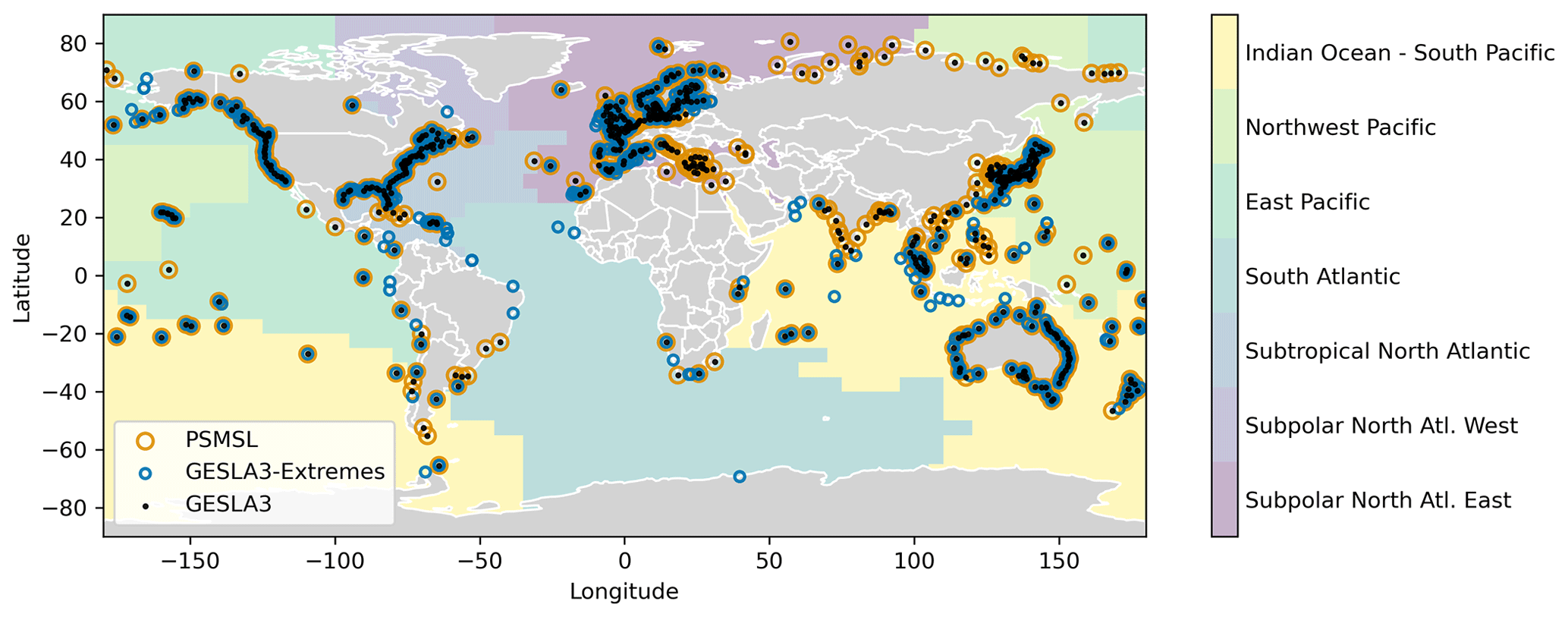
Figure 1Tide gauge stations used for the evaluation of the presented dataset. Orange circles show 663 tide gauge stations from PSMSL, black dots show 1040 tide gauge stations from the GESLA-3 database with 30 % data coverage in the period 1979 to 2015 and blue circles show 999 GESLA-3 stations that have at least 90 % data coverage in the period 2011–2015. The respective ocean basins are shown as colored areas. Map adapted from Thompson and Merrifield (2014) with an additional division of the North Atlantic into West and East and are extended by nearest-neighbor interpolation.
The second analysis is based on storm surge time series from GESLA-3. To remove the tidal contribution we estimate tides for the observations by fitting harmonic functions with 69 harmonic components as described by Annunziato and Probst (2016). To preserve variability with frequencies that are larger than or equal to 1 month, we predict harmonic tides based on fitted parameters for 65 sub-monthly harmonic components only, leaving out 4 components with frequencies larger than or equal to 1 month. We then remove the predicted harmonic tides from the observations.
We evaluate the performance of HCC on the 99th percentile of daily maxima storm surge in the 2011–2015 period. To that end, we vertically align the observational and factual datasets by removing their respective mean value for time steps with valid observations in this period. We require at least 90 % data coverage in this period. With these restrictions we use 999 tide gauge records from GESLA-3 for this analysis. In Text S1 and Fig. S1 in the Supplement, we perform a statistical test on how sensitive the vertical alignment is on different percentages of data coverage in the alignment period.
The tide gauge stations used in this study are illustrated in Fig. 1, with colors referring to ocean basins following the definition of Thompson and Merrifield (2014).
2.5 Counterfactual water levels
We generate counterfactual water levels that exclude the trends since the beginning of the 20th century but preserve the short-term sea level variability of the factual dataset. There is increased evidence for an acceleration in global sea level rise (Church and White, 2011; Hay et al., 2015; Frederikse et al., 2020; Dangendorf et al., 2017, 2019). To account for the accelerated trend in sea level rise, we employ a quadratic trend model. For each location, we estimate this trend using linear regression on the annual mean time series, setting the intercept to the average sea level from 1900–1905. After removing this long-term trend, we obtain the counterfactual time series. We evaluate the robustness of this trend estimate using the moving block bootstrapping algorithm, as described by Mudelsee (2019). We find that the total sea level rise derived from the trend estimate varies depending on the location, with standard deviations ranging from 3.4 to 16.7 mm and an average standard deviation of 8.1 mm (See supplement Text S2 and Fig. S2). While uncertainties exist, this demonstrates that the quadratic model provides a robust representation of the long-term trend in sea level rise. Importantly, the uncertainty associated with our model is relatively small when compared to the uncertainties in the factual dataset itself.
As the water height relative to the coast is needed as input for impact models, the factual/counterfactual pair can be used as forcing in such models directly. We additionally provide a counterfactual of the geocentric version of the factual dataset excluding the effects of VLM. The geocentric factual/counterfactual pair can be used if it is known from other sources that VLM is negligible or if better VLM estimates are available regionally. To yield a counterfactual consistent with our approach, the VLM quadratic trend since 1900–1905 would need to be estimated from the regional VLM data and then subtracted from the geocentric counterfactual dataset.
We provide the factual and counterfactual datasets with hourly resolution for the time period 1979–2015 and monthly resolution for the time period 1900–2015.
Table 1RMSE in centimeters between tide gauge observations and different reconstructions of coastal water levels. For the comparison on daily maximum values, time series are detrended by removing annual means (marked with an * in the table header). Rows contain median and standard deviation (in brackets) of RMSE in centimeters, aggregated for different basins and globally. The rightmost column shows median bias of the top 1 % daily maximum surge levels between HCC and tide gauge observations. Negative values indicate that HCC underestimates the observed surge level.
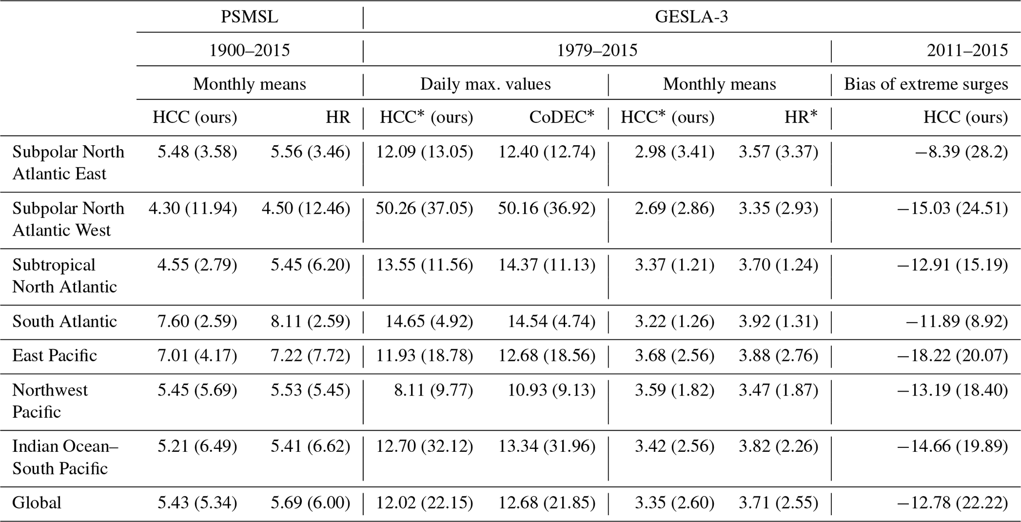
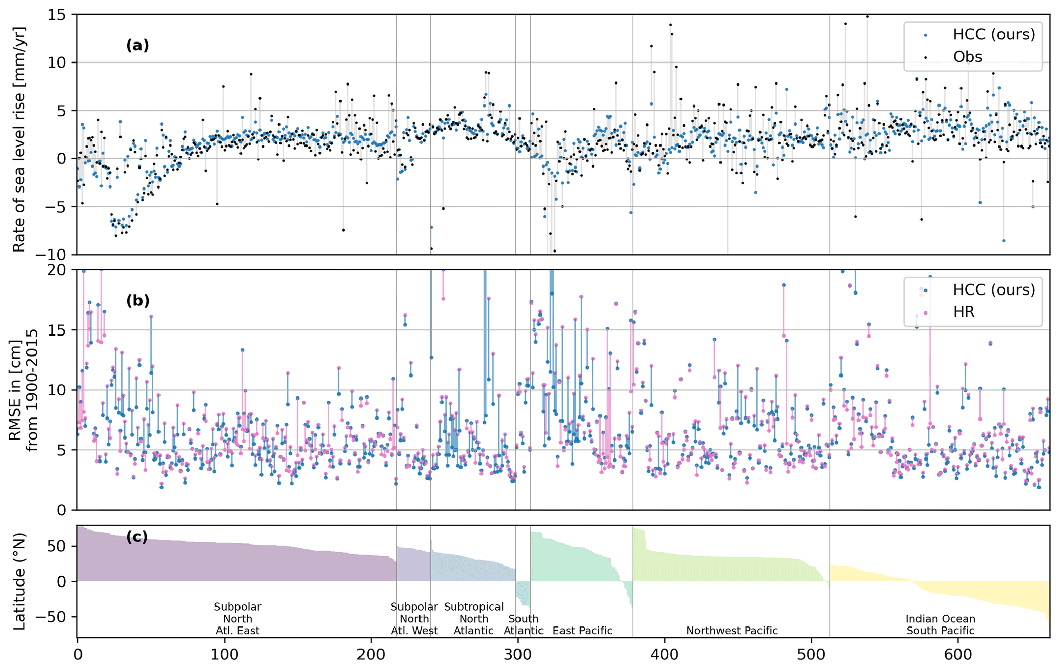
Figure 2Performance of our HCC dataset and the HR dataset compared to tide gauges from the PSMSL record. (a) Linear sea level trend for years with valid observations for tide gauge records (black) and HCC (blue) connected by a gray bar. (b) RMSE between observed and modeled RSL as blue and pink dots for HCC and HR respectively. RMSE values for the same tide gauge station are connected with a blue bar if HCC has a lower RMSE than HR and with a pink bar if it is higher. (c) Latitude of tide gauge locations sorted by ocean basin. A progressive integer of the considered tide gauge is plotted on the x axis. Outliers are not plotted.
3.1 Long-term sea level trends
We evaluate the performance of our dataset by comparing it to tide gauge measurements from the PSMSL database. In the “Materials and methods” section we describe in more detail how we select tide gauge measurements from PSMSL and how we align it with the HCC and HR datasets. To visualize long-term sea level change we plot the linear trend from the tide gauge records and the modeled coastal water levels respectively for years with valid observations. Our dataset reflects the different trends in different world regions well (Fig. 2a) and shows a comparable RMSE against observations. Figure 2b shows the RMSE of the monthly HCC dataset and the HR dataset against observations. Figure 2c depicts latitudes for all tide gauge stations from the PSMSL record that were used to analyze monthly water levels, aligned by ocean basins.
We evaluate the performance of the HCC dataset through its RMSE against observations and compare it to the performance of the HR dataset (Table 1). The HCC dataset shows a median RMSE of 5.43 cm (SD 5.34 cm) over all tide gauge stations, which is an improvement compared to the HR, with a median RMSE of 5.69 cm (SD 6.00 cm). We performed a Wilcoxon signed-rank test to compare the RMSE samples and found that the improvement is statistically significant, with a p value of . However, the improvement of 0.26 cm is only modest when compared to the total error magnitudes. The improvement occurs in all seven basins and is pronounced in the Subtropical North Atlantic, with a median RMSE of 4.55 cm (SD 2.79 cm) as compared to 5.45 cm (SD 6.2 cm) in HR. Figure 2b provides more detail, showing RMSE per tide gauge. In the higher latitudes of the East Pacific, our dataset has a lower RMSE than HR for most stations (Fig. 2b). The performance also decreases at tide gauges in the lower northern latitudes of the East Pacific. As these regions are all located at plate boundaries and are thus highly prone to tectonically induced VLM, this may hint at problems in the extrapolation back in time to 1900 from recent VLM data for such regions. However, in summary, for all locations we see the inclusion of observational VLM and its backward extrapolation superior to approaches that only include the GIA component of VLM and neglect other contributing processes, as can be seen in the overall improvement of median RMSE.
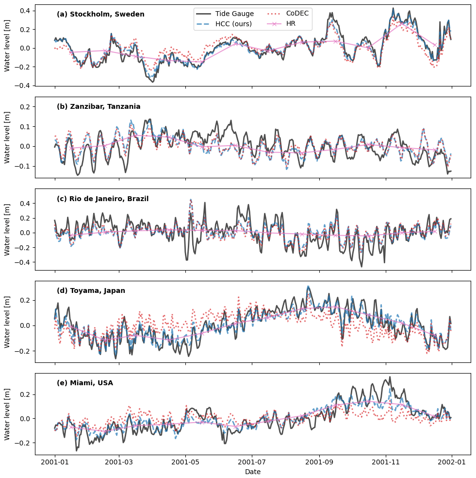
Figure 3Illustrative comparison of our HCC (blue line), the HR (pink line) and CoDEC (red line) datasets with observations (black line) at five example tide gauge stations. We show daily mean values for the year 2001 that are vertically aligned by removing the respective annual mean sea level.
3.2 Intra-annual variability
To evaluate our dataset on timescales shorter than a year, we compare it with observations from the GESLA-3 database. For illustration, in Fig. 3 we first show daily mean values for CoDEC, HR and our dataset as anomalies to their respective yearly mean in the year 2001 for five selected tide gauge stations. For the example of Stockholm, Sweden, the density variations modulating sea level during the annual cycle as present in HR bring the atmospheric wind- and pressure-driven variability from CoDEC significantly closer to observations and thus improve the performance in our combined dataset. A similar effect is evident for Toyama, Japan, and Miami, USA. Notably, also after including HR, the HCC water levels do not perfectly match the observations. Discrepancies remain, e.g., in Miami, USA, between October and November 2001. However this falls well within the uncertainty margins of the HR dataset, given that it represents a global statistical reconstruction of water levels. For the stations of Zanzibar, Tanzania, and Rio de Janeiro, Brazil, sea level variation of HR is low as compared to the total sea level amplitude; thus the factual dataset and CoDEC evolve similarly, and an improvement is not evident. Both stations are located in areas that are barely covered by tide gauges used in HR.
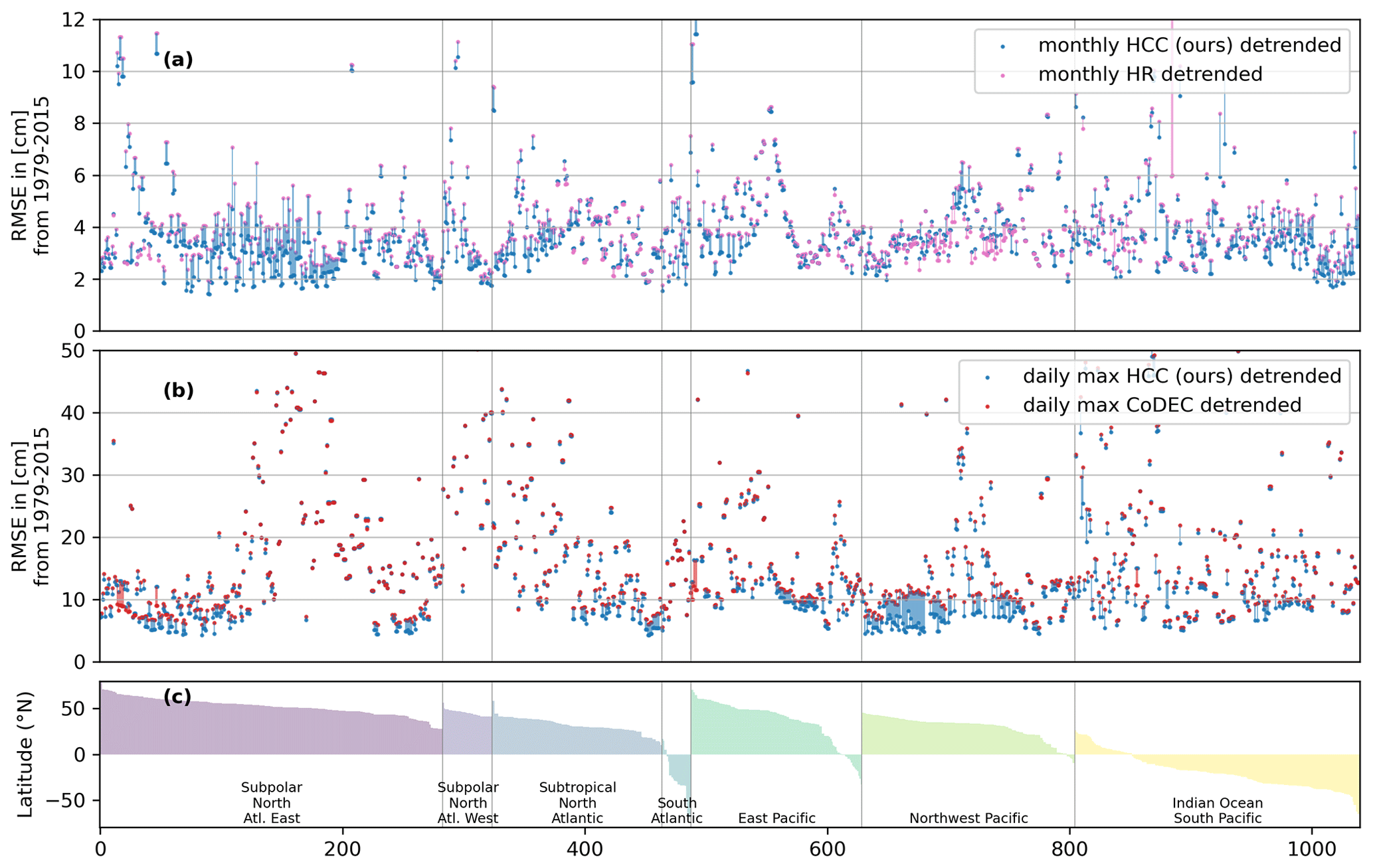
Figure 4Comparison between our HCC dataset, HR, CoDEC and tide gauge records from GESLA-3. (a) RMSE of monthly mean sea level between HCC and GESLA-3 (blue dots) and HR and GESLA-3 (pink dots). Dots are connected with a blue bar if monthly HCC has a lower RMSE than HR and with a pink bar if it has a higher RMSE. (b) RMSE between annually detrended HCC and GESLA-3 (blue dots) and annually detrended CoDEC and GESLA-3 (red dots). Dots connected analogously to (a). (c) Latitude of tide gauge locations sorted by ocean basin. A progressive integer of the considered tide gauge is plotted on the x axis. Outliers are not plotted.
We assess if improvements are visible over all tide gauges in Fig. 4. We compare coastal water levels from our dataset, CoDEC and HR through their respective RMSE against tide gauge observations. Following Muis et al. (2020), each dataset is detrended by subtracting the annual mean from each time series and each year respectively. This means that a performance improvement is due to better alignment of intra-annual variability with tide gauges as inter-annual mean sea level change is explicitly excluded. For most locations the RMSE against tide gauge observations from GESLA-3 is lower for our detrended monthly dataset than for HR, visualized by blue bars in Fig. 4a. The global median RMSE of our dataset is 3.35 cm (SD 2.60 cm) compared to 3.71 cm (SD 2.55 cm) for the HR dataset. The improvement is consistent over all basins except for the Northwest Pacific, where the median RMSE for our dataset of 3.59 cm (SD 1.82 cm) is slightly higher than for HR with 3.47 cm (SD 1.87 cm) (Table 1). The improved performance of our dataset is stronger in midlatitudes to higher latitudes of the North Atlantic and some stations in the East Pacific. In the East Pacific and Indian Ocean–South Pacific, there is a mixed picture, with some stations showing a lower performance than HR (green bars Fig. 4a). Wind-driven and air-pressure-driven barotropic sea level variability is more pronounced in midlatitudes to higher latitudes (Merrifield et al., 2013), which might explain the improved performance of our dataset in these regions since it uses sea level variability from CoDEC on a timescale up to 3 months. This is plausible as wind-driven variability and air-pressure-driven sea level variability are explicitly modeled in CoDEC and only interpolated from sparse observations in HR. Daily maximum water levels in our dataset have a global median RMSE of 12.02 cm (SD 22.15 cm), which is lower compared to CoDEC, with a median RMSE of 12.68 cm (SD 21.85 cm). This improvement is evident for almost all stations, as illustrated by the blue bars in Fig. 4b. The largest performance increases are in the Northwest Pacific where our dataset has a median RMSE of 8.11 cm (SD 9.77 cm) compared to 10.93 cm (SD 9.13 cm) for CoDEC and is almost halved to values as low as 50 mm for some stations (Fig. 4b). The more important role of ocean density variations as compared to wind-driven and air-pressure-driven variability is a plausible explanation for the stronger increase in performance in the lower latitudes. Density variations are captured in our dataset through the inclusion of HR and the seasonal cycle from AVISO.
3.3 Extreme water levels
To illustrate the role of the long-term trend in sea level extremes, we investigate extreme water levels in our factual and counterfactual dataset and compare them to tide gauge observations from GESLA-3. We only consider extreme events from 2011–2015 because this period is covered well in the observations, and sea level rise is close to its maximum. We restrict our analysis of extreme water levels to tide gauge stations with at least 90 % of data in the considered period which leaves a total of 999 stations. As astronomical tides introduce a strong offset in extreme water levels and thus make the comparison between different locations difficult, here we remove astronomical tides from the modeled and observed water levels and focus on the surge component. As coasts are historically adapted to their tides, extreme surges are an important cause for extreme impact events and their damages. We therefore analyze the 99th percentile of daily maximum surge levels. To that end, we pick the 1 % highest daily maximum surge levels from the observational data in the years 2011–2015 and compare those to our factual and counterfactual dataset. We focus solely on sea level anomalies, to level out differences in surge height between different stations, caused by permanent differences to the geoid. We calculate sea level anomalies for tide gauge records by removing the mean sea level over time steps with valid observations in the period 2011–2015. To reduce the alignment error, we calculate the mean sea level for the factual dataset only for time steps with valid observations in the tide gauge record. From that we derive sea level anomalies for the factual and counterfactual by removing the factual mean sea level from both datasets. This maintains the difference between the factual and counterfactual datasets resulting from long-term sea level rise.
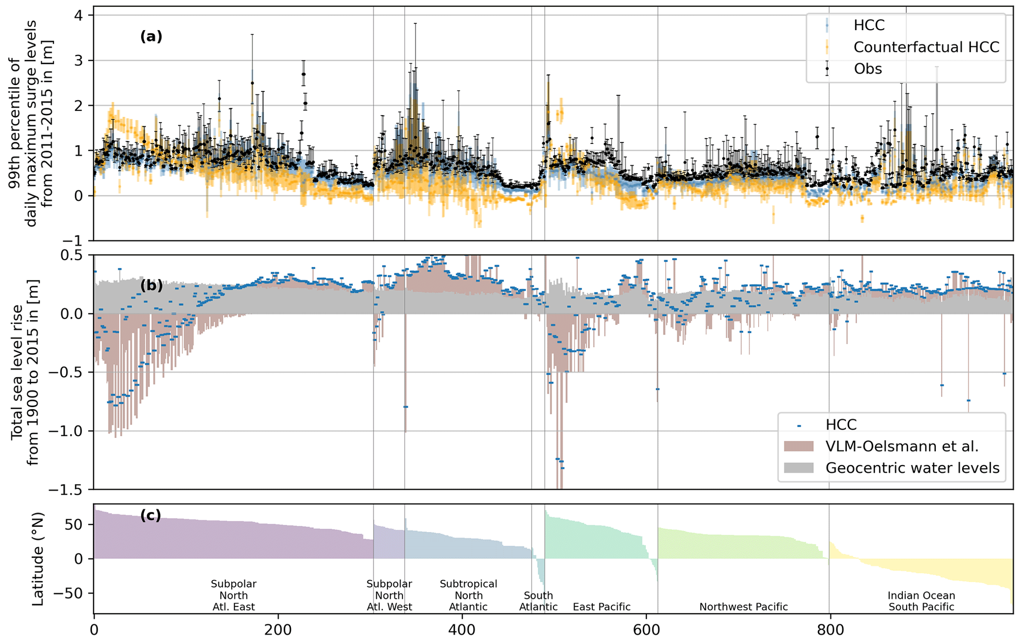
Figure 5Range and mean of the top 1 % of extreme coastal water levels without astronomical tides for tide gauge observations (black) and our factual (blue) and our counterfactual (orange) HCC data (a). The mean value of the factual HCC data from 2011–2015 is subtracted from all three datasets. Panel (b) shows mean coastal water level change from 1900 to 2015, computed by subtracting the mean value over 2010–2015 from the mean value over 1900 to 1905. Blue markers show coastal water level change for the presented dataset and is decomposed into the geocentric component (gray bars) and the contribution of VLM (brown bars). Latitude of tide gauge locations sorted by ocean basin (c). A progressive integer of the considered tide gauge is plotted on the x axis. Outliers are not plotted.
We show these top 1 % highest water levels for our factual and counterfactual dataset and the tide gauge observations in Fig. 5a. In general, there is a good agreement between modeled extreme water levels (blue bars) and observations (black markers). However, our dataset underestimates the extreme water levels at most locations, with a median bias of −12.78 cm (SD 22.22 cm). This underestimation is pronounced for the East Pacific with −18.22 cm (SD 20.07 cm) and Subpolar North Atlantic West with −15.03 cm (SD 24.51 cm) (Table 1). There is a known low bias in the model, in particular for the highest water levels originating from the CoDEC dataset. It is largely attributed to the spatial resolution of the atmospheric inputs (Muis et al., 2020).
By design, the counterfactual dataset preserves the daily, monthly and inter-annual variability of the factual dataset. Extreme sea level events have the same timing in the counterfactual and the factual. We can thus pick the timings of the 1 % highest water levels from the factual dataset and assess the events in the counterfactual dataset in Fig. 5a. The trend in relative coastal water levels increased extreme water levels for almost all world regions with the counterfactual lying below the factual for most tide gauge locations. In particular, for regions with low surge magnitudes, it often contributes a significant fraction to the extreme event. The situation is different for the high northern latitudes where counterfactual sea level rise is above the factual. In these regions the extreme event magnitude is reduced, primarily due to the influence of GIA (Emery and Aubrey, 1985). In some regions the counterfactual is below zero. These are regions where the highest surge levels are close to the mean sea level from 2011–2015. With the factual not much higher than zero, the counterfactual without the sea level trend since 1900 easily falls below zero.
We illustrate the contribution from geocentric water levels and VLM to the relative coastal water levels in Fig. 5b. The contribution of geocentric water levels is relatively stable across locations. This is in contrast to the contribution from VLM, which is more variable across locations. In many places both processes have a similar order of magnitude, and there are some regions where VLM exceeds changes in geocentric water levels. This has been recognized in earlier works (Oelsmann et al., 2024; Nicholls et al., 2021; Pfeffer et al., 2017; Hawkins et al., 2019b; Hammond et al., 2021; Wöppelmann and Marcos, 2016).
The HCC dataset is made available openly through the Inter-Sectoral Impact Model Intercomparison Project (ISIMIP) at https://doi.org/10.48364/ISIMIP.749905 (Treu et al., 2023a). The source code (v1.1) underlying the analysis and producing the figures presented in the paper is archived at https://doi.org/10.5281/zenodo.10359838 (Treu, 2023). All code is open to use under the Creative Commons Attribution 4.0 International license.
We provide direct links to all datasets used in this study:
-
CoDEC and HR – https://doi.org/10.5281/zenodo.8322750 (Muis et al., 2023);
-
VLM – https://doi.org/10.5281/zenodo.8308347 (Oelsmann et al., 2023);
-
PSMSL tide gauge data (PSMSL, 2022; Holgate et al., 2013), retrieved on 26 September 2022 from https://psmsl.org/data/optaining/year_end/2022 (last access: 21 February 2024);
-
GESLA-3 tide gauge data (Haigh et al, 2022a, b), retrieved on 23 August 2023 from https://gesla787883612.wordpress.com/downloads/ (last access: 21 February 2024).
We use two different sources of satellite altimetry:
-
To separate the seasonal cycle from HR, we use the same satellite altimetry dataset that was employed in the production of HR. The dataset is a merged product of TOPEX/Poseidon and Jason altimeter missions and was at that time distributed by AVISO. This dataset, including the corrections described in Dangendorf et al. (2019), is archived together with the HR dataset at https://doi.org/10.5281/zenodo.8322750 (Muis et al., 2023).
-
To reference our dataset to the WGS 84 geoid, we use the CMEMS mean dynamic topography dataset SEALEVEL_GLO_PHY_MDT_008_063, available at https://doi.org/10.48670/moi-00150 (E.U. Copernicus Marine Service Information (CMEMS), 2024).
Data and code used to produce the table and figures presented in this study, based on v1.2 of the source code, are archived at https://doi.org/10.5281/zenodo.10354898 (Treu et al., 2023b).
In this work, we combine datasets of long-term sea level change, short-term coastal water level variability and VLM to yield a forcing dataset for historical simulations with coastal impact models. To facilitate the attribution of historical impacts to sea level rise, we complement the dataset with a counterfactual.
The task poses several challenges. A major one is the inclusion of VLM to yield relative coastal water levels. Given the sparsity of direct observational data, particularly prior to the 1990s, extrapolating VLM back to the early 20th century makes our estimates error prone, and anthropogenic influence post-WWII adds additional difficulties. It is difficult to exclude anthropogenic influences like fluid extraction from the trend estimation. Further advances in this field should be incorporated in future sea level assessments. By providing a geocentric version of the HCC dataset, it is possible to combine our water levels with other reconstructions of VLM.
Another challenge originates from the different nature of the source datasets that we combine. HR and the VLM data are built from observations; thus they include all contributing processes, but there are limits for the disentanglement of components in these datasets. CoDEC is a simulation-based dataset in which the individual components are available, but CoDEC does not capture all processes. We avoid double counting atmospherically driven barotropic sea level changes by frequency filtering, which affects all processes. The choice of a specific cutoff frequency is a trade-off as it means that processes with higher frequencies come from the CoDEC dataset without coverage of density-driven sea level variability. Partly, we can account for that by frequency filtering only deseasonalized data and adding the seasonal cycle from AVISO satellite altimetry. For processes with lower frequencies than the cutoff, sea level variability comes from HR which covers density-driven variability but is for many regions not as good at covering atmospherically driven variability as CoDEC. Future work could explore using region-specific cutoff frequencies to better harness the individual strengths of HR and CoDEC. This approach, however, would necessitate a comprehensive analysis of the dominant timescales of variability within each dataset for different regions.
HR does not cover regions with sea ice because there is no continuous coverage of altimetry for those regions. Our coastal water levels in those regions are based on extrapolation of HR and need to be used with extreme care. We provide a mask along with the dataset so users can exclude sea ice areas. For some of these regions, namely for Greenland, Siberia and Antarctica, VLM data are also absent (Oelsmann et al., 2024).
To derive a counterfactual dataset in line with the concept of impact attribution of the IPCC, we use a quadratic model to first estimate and then remove the sea level trend since 1900 from the factual dataset. The quadratic model assumes a constant acceleration of sea level rise over time. Analysis of sea level rise shows variation throughout the last century, with an acceleration phase early in the century, followed by a deceleration and then again an acceleration until today (Frederikse et al., 2020; Dangendorf et al., 2019; Slangen et al., 2016). By design, this variation is not included in our quadratic trend estimate. In general, we expect our trend estimation to largely exclude natural variability due to its low dimension and the long data period. This is a desired outcome and preserves the natural variability in the counterfactual. The quadratic model provides robust trend estimates, given the fact that we do not extrapolate the trend into the future, which would increase uncertainties. To further increase the robustness of the trend estimate, future studies should include predictors for the main modes of climate variability as, for example, in Menéndez and Woodworth (2010), Marcos and Woodworth (2017), and Wang et al. (2021).
In contrast to atmospheric climate change, there is no pre-industrial period in which sea level was stable over time. There is therefore not a clear indication for the time period that we can reference as the baseline for the counterfactual. Here we took the practical choice of making the years 1900–1905 the reference time because this is when the HR dataset starts. In a strict sense, with the counterfactual forcing data, we thus mimic a sea level world of the beginning of the 20th century and not a world in which sea level rise has not occurred. The approach produces counterfactuals that are largely stationary but incorporates the same shorter-term variability as the factual dataset. The data thus also allow for impact attribution of individual coastal extreme events. For an extended discussion of the concept, see Mengel et al. (2021).
Without additional analysis, the presented work does not allow for the attribution of coastal impacts to anthropogenic greenhouse gas emissions, mediated through sea level rise. Such additional steps would need the differentiation between climate variability and forced climate response. This is usually done via large model ensembles and dedicated experimental setups like DAMIP (Gillett et al., 2016). While attribution of global mean sea level change to anthropogenic emissions is possible (e.g., Slangen et al., 2016), the task of separating variability from the forced signal is more challenging on the regional level that is necessary for impact assessments and not yet possible over the 20th century (Fox-Kemper et al., 2021). Here we deliberately exclude the separation of anthropogenic and non-anthropogenic forcing of sea level rise as it often becomes the focus of impact attribution studies and sidelines the more difficult and less researched but, in our view, very relevant issue of separation of climate change from direct human interventions as drivers of observed changes in natural, human and managed systems. Additionally, large Earth system model ensembles that would allow for the attribution to emissions but also reliably capture all major sea level components are not available so far.
We provide the factual and counterfactual dataset as part of the ISIMIP3a simulation round. This simulation round is dedicated to the evaluation of impact models and to impact attribution. ISIMIP already provides datasets on some additional drivers of coastal impacts, such as change in population, land use, economy or urban area2. With the presented data, we aim to facilitate the development of a new generation of coastal impact models that explicitly resolve the observed spatial and temporal coastal changes and disturbances.
The supplement related to this article is available online at: https://doi.org/10.5194/essd-16-1121-2024-supplement.
ST and MM developed the concept. ST implemented the methods, wrote the code and produced the data. SD, SM, TW and JO provided the input data. All authors contributed to the writing of the manuscript.
The contact author has declared that none of the authors has any competing interests.
Publisher’s note: Copernicus Publications remains neutral with regard to jurisdictional claims made in the text, published maps, institutional affiliations, or any other geographical representation in this paper. While Copernicus Publications makes every effort to include appropriate place names, the final responsibility lies with the authors.
This study has been conducted using EU Copernicus Marine Service Information; https://doi.org/10.48670/moi-00150.
This research has been supported by the Bundesministerium für Bildung, Wissenschaft, Forschung und Technologie (grant nos. 01LP1907A and 16QK05), the European Commission, Horizon 2020 (grant no. 820712), and the European Cooperation in Science and Technology (grant no. CA19139).
Thomas Wahl has been supported by NASA’s Sea Level Change Team (award number 80NSSC20K1241) and the National Science Foundation (award numbers 1854896 and 2141461). Sönke Dangendorf has been supported by NASA’s Sea Level Change Team (award number 80NSSC20K1241) and David and Jane Flowerree.
The publication of this article was funded by the Open Access Fund of the Leibniz Association.
This paper was edited by Simona Simoncelli and reviewed by Matteo Meli and one anonymous referee.
Albert, S., Leon, J. X., Grinham, A. R., Church, J. A., Gibbes, B. R., and Woodroffe, C. D.: Interactions between sea-level rise and wave exposure on reef island dynamics in the Solomon Islands, Environ. Res. Lett., 11, 054011, https://doi.org/10.1088/1748-9326/11/5/054011, 2016.
Annunziato, A. and Probst, P.: Continuous Harmonics Analysis of Sea Level Measurements: Description of a new method to determine sea level measurement tidal component, EUR 28308 EN, Ispra (Italy), Publications Office of the European Union, JRC104684, 2016.
Brown, S., Nicholls, R. J., Goodwin, P., Haigh, I. D., Lincke, D., Vafeidis, A. T., and Hinkel, J.: Quantifying land and people exposed to sea-level rise with no mitigation and 1.5° C and 2.0° C rise in global temperatures to year 2300, Earths Future, 6, 583–600, 2018.
Caldwell, P. C., Merrifield, M. A., and Thompson, P. R.: Sea level measured by tide gauges from global oceans – the Joint Archive for Sea Level holdings (NCEI Accession 0019568), Version 5.5, NOAA National Centers for Environmental Information [data set], https://doi.org/10.7289/V5V40S7W, 2015.
Caron, L., Ivins, E. R., Larour, E., Adhikari, S., Nilsson, J., and Blewitt, G.: GIA Model Statistics for GRACE Hydrology, Cryosphere, and Ocean Science, Geophys. Res. Lett., 45, 2203–2212, https://doi.org/10.1002/2017GL076644, 2018.
Church, J. A. and White, N. J.: Sea-Level Rise from the Late 19th to the Early 21st Century, Surv. Geophys., 32, 585–602, 2011.
Church, J. A., White, N. J., Konikow, L. F., Domingues, C. M., Cogley, J. G., Rignot, E., Gregory, J. M., van den Broeke, M. R., Monaghan, A. J., and Velicogna, I.: Revisiting the Earth's sea-level and energy budgets from 1961 to 2008, Geophys. Res. Lett., 38, L18601, https://doi.org/10.1029/2011gl048794, 2011.
Dangendorf, S., Calafat, F. M., Arns, A., Wahl, T., Haigh, I. D., and Jensen, J.: Mean sea level variability in the North Sea: Processes and implications, J. Geophys. Res.-Oceans, 119, 6820–6841, https://doi.org/10.1002/2014JC009901, 2014.
Dangendorf, S., Marcos, M., Wöppelmann, G., Conrad, C. P., Frederikse, T., and Riva, R.: Reassessment of 20th century global mean sea level rise, P. Natl. Acad. Sci. USA, 114, 5946–5951, 2017.
Dangendorf, S., Hay, C., Calafat, F. M., Marcos, M., Piecuch, C. G., Berk, K., and Jensen, J.: Persistent acceleration in global sea-level rise since the 1960s, Nat. Clim. Change, 9, 705–710, 2019.
Dangendorf, S., Frederikse, T., Chafik, L., Klinck, J. M., Ezer, T., and Hamlington, B. D.: Data-driven reconstruction reveals large-scale ocean circulation control on coastal sea level, Nat. Clim. Change, 11, 514–520, 2021.
Dullaart, J. C. M., Muis, S., Bloemendaal, N., and Aerts, J. C. J. H.: Advancing global storm surge modelling using the new ERA5 climate reanalysis, Clim. Dynam., 54, 1007–1021, 2020.
Emery, K. O. and Aubrey, D. G.: Glacial rebound and relative sea levels in Europe from tide-gauge records, Tectonophysics, 120, 239–255, 1985.
Enríquez-de-Salamanca, Á.: Evolution of coastal erosion in Palmarin (Senegal), J. Coast. Conserv., 24, 25, 1874–7841, https://doi.org/10.1007/s11852-020-00742-y, 2020.
E.U. Copernicus Marine Service Information (CMEMS): Global Ocean Mean Dynamic Topography SEALEVEL_GLO_PHY_MDT_008_063, Marine Data Store (MDS) [data set], https://doi.org/10.48670/moi-00150, 2024.
Fox-Kemper, B., Hewitt, H. T., Xiao, C., Aðalgeirsdóttir, G., Drijfhout, S. S., Edwards, T. L., Golledge, N. R., Hemer, M., Kopp, R. E., Krinner, G., Mix, A., Notz, D., Nowicki, S., Nurhati, I. S., Ruiz, L., Sallée, J.-B., Slangen, A. B. A., and Yu, A. Y.: Ocean, Cryosphere and Sea Level Change, in: Climate Change 2021: The Physical Science Basis. Contribution of Working Group I to the Sixth Assessment Report of the Intergovernmental Panel on Climate Change, edited by: MassonDelmotte, V., Zhai, P., Pirani, A., Connors, S. L., Péan, C., Berger, S., Caud, N., Chen, Y., Goldfarb, L., Gomis, M. I., Huang, M., Leitzell, K., Lonnoy, E., Matthews, J. B. R., Maycock, T. K., Waterfield, T., Yelekçi, O., Yu, R., and Zhou, B., Cambridge University Press, 1211–1362, https://doi.org/10.1017/9781009157896.011, 2021.
Frederikse, T., Landerer, F., Caron, L., Adhikari, S., Parkes, D., Humphrey, V. W., Dangendorf, S., Hogarth, P., Zanna, L., Cheng, L., and Wu, Y.-H.: The causes of sea-level rise since 1900, Nature, 584, 393–397, 2020.
Gesch, D. B.: Best Practices for Elevation-Based Assessments of Sea-Level Rise and Coastal Flooding Exposure, Front Earth Sci. Chin., 6, 230, https://doi.org/10.3389/feart.2018.00230, 2018.
Gillett, N. P., Shiogama, H., Funke, B., Hegerl, G., Knutti, R., Matthes, K., Santer, B. D., Stone, D., and Tebaldi, C.: The Detection and Attribution Model Intercomparison Project (DAMIP v1.0) contribution to CMIP6, Geosci. Model Dev., 9, 3685–3697, https://doi.org/10.5194/gmd-9-3685-2016, 2016.
Haigh, I., Marcos Moreno, M., Talke, S., Woodworth, P., Hunter, J., Hague, B., Arns, A., Bradshaw, E., and Thompson, P.: The Global Extreme Sea Level Analysis (GESLA) Version 3 dataset: Part 1, NERC EDS British Oceanographic Data Centre NOC [data set], https://doi.org/10.5285/d21a496a-a48e-1f21-e053-6c86abc08512, 2022a.
Haigh, I., Marcos Moreno, M., Talke, S., Woodworth, P., Hunter, J., Hague, B., Arns, A., Bradshaw, E., and Thompson, P.: The Global Extreme Sea Level Analysis (GESLA) Version 3 dataset: Part 2, NERC EDS British Oceanographic Data Centre NOC [data set], https://doi.org/10.5285/d21a496a-a48f-1f21-e053-6c86abc08512, 2022b.
Haigh, I. D., Marcos, M., Talke, S. A., Woodworth, P. L., Hunter, J. R., Hague, B. S., Arns, A., Bradshaw, E., and Thompson, P.: GESLA Version 3: A major update to the global higher-frequency sea-level dataset, Geosci. Data J., 10, 293–314, 2023.
Hallegatte, S., Green, C., Nicholls, R. J., and Corfee-Morlot, J.: Future flood losses in major coastal cities, Nat. Clim. Change, 3, 802–806, https://doi.org/10.1038/nclimate1979, 2013.
Hammond, W. C., Blewitt, G., Kreemer, C., and Nerem, R. S.: GPS Imaging of Global Vertical Land Motion for Studies of Sea Level Rise, J. Geophys. Res.-Sol. Ea., 126, e2021JB022355, https://doi.org/10.1029/2021JB022355, 2021.
Hawkins, R., Bodin, T., Sambridge, M., Choblet, G., and Husson, L.: Trans-dimensional surface reconstruction with different classes of parameterization, Geochem. Geophy. Geosy., 20, 505–529, 2019a.
Hawkins, R., Husson, L., Choblet, G., Bodin, T., and Pfeffer, J.: Virtual tide gauges for predicting relative sea level rise, J. Geophys. Res.-Sol. Ea., 124, 13367–13391, 2019b.
Hay, C. C., Morrow, E., Kopp, R. E., and Mitrovica, J. X.: Probabilistic reanalysis of twentieth-century sea-level rise, Nature, 517, 481–484, https://doi.org/10.1038/nature14093, 2015.
Hersbach, H., Bell, B., Berrisford, P., Hirahara, S., Horányi, A., Muñoz-Sabater, J., Nicolas, J., Peubey, C., Radu, R., Schepers, D., Simmons, A., Soci, C., Abdalla, S., Abellan, X., Balsamo, G., Bechtold, P., Biavati, G., Bidlot, J., Bonavita, M., Chiara, G., Dahlgren, P., Dee, D., Diamantakis, M., Dragani, R., Flemming, J., Forbes, R., Fuentes, M., Geer, A., Haimberger, L., Healy, S., Hogan, R. J., Hólm, E., Janisková, M., Keeley, S., Laloyaux, P., Lopez, P., Lupu, C., Radnoti, G., Rosnay, P., Rozum, I., Vamborg, F., Villaume, S., and Thépaut, J.: The ERA5 global reanalysis, Q. J. Roy. Meteor. Soc., 146, 1999–2049, 2020.
Hinkel, J., Lincke, D., Vafeidis, A. T., Perrette, M., Nicholls, R. J., Tol, R. S. J., Marzeion, B., Fettweis, X., Ionescu, C., and Levermann, A.: Coastal flood damage and adaptation costs under 21st century sea-level rise, P. Natl. Acad. Sci. USA, 111, 3292–3297, 2014.
Holgate, S. J., Matthews, A., Woodworth, P. L., Rickards, L. J., Tamisiea, M. E., Bradshaw, E., Foden, P. R., Gordon, K. M., Jevrejeva, S., and Pugh, J.: New Data Systems and Products at the Permanent Service for Mean Sea Level, coas, 29, 493–504, https://doi.org/10.2112/JCOASTRES-D-12-00175.1, 2013.
Hooijer, A. and Vernimmen, R.: Global LiDAR land elevation data reveal greatest sea-level rise vulnerability in the tropics, Nat. Commun., 12, 3592, https://doi.org/10.1038/s41467-021-23810-9, 2021.
Hope, P., Cramer, W., van Aalst, M., Flato, G., Frieler, K., Gillett, N., Huggel, C., Minx, J., Otto, F., Parmesan, C., Rogelj, J., Rojas, M., Seneviratne, S. I., Slangen, A., Stone, D., Terray, L., Vautard, R., and Zhang, X.: Cross-Working Group Box ATTRIBUTION, in: Climate Change 2022: Impacts, Adaptation and Vulnerability. Contribution of Working Group II to the Sixth Assessment Report of the Intergovernmental Panel on Climate Change, edited by: Pörtner, H. O., Roberts, D. C., Tignor, M., Poloczanska, E. S., Mintenbeck, K., Alegría, A., Craig, M., Langsdorf, S., Löschke, S., Möller, V., Okem, A., and Rama, B., Cambridge University Press, Cambridge, UK and New York, USA, 121–196, https://doi.org/10.1017/9781009325844, 2022.
Hunter, J. R., Woodworth, P. L., Wahl, T., and Nicholls, R. J.: Using global tide gauge data to validate and improve the representation of extreme sea levels in flood impact studies, Global Planet. Change, 156, 34–45, 2017.
Irish, J. L., Sleath, A., Cialone, M. A., Knutson, T. R., and Jensen, R. E.: Simulations of Hurricane Katrina (2005) under sea level and climate conditions for 1900, Clim. Change, 122, 635–649, 2014.
Kanwal, S., Ding, X., Sajjad, M., and Abbas, S.: Three Decades of Coastal Changes in Sindh, Pakistan (1989–2018): A Geospatial Assessment, Remote Sensing, 12, 8, https://doi.org/10.3390/rs12010008, 2020.
Kernkamp, H. W. J., Van Dam, A., Stelling, G. S., and de Goede, E. D.: Efficient scheme for the shallow water equations on unstructured grids with application to the Continental Shelf, Ocean Dynam., 61, 1175–1188, 2011.
Kirezci, E., Young, I. R., Ranasinghe, R., Lincke, D., and Hinkel, J.: Global-scale analysis of socioeconomic impacts of coastal flooding over the 21st century, Front. Mar. Sci., 9, 1024111, https://doi.org/10.3389/fmars.2022.1024111, 2023.
Kopp, R. E., Horton, R. M., Little, C. M., Mitrovica, J. X., Oppenheimer, M., Rasmussen, D. J., Strauss, B. H., and Tebaldi, C.: Probabilistic 21st and 22nd century sea-level projections at a global network of tide-gauge sites, Earth's Future, 2, 383–406, https://doi.org/10.1002/2014ef000239, 2014.
Lin, N., Kopp, R. E., Horton, B. P., and Donnelly, J. P.: Hurricane Sandy's flood frequency increasing from year 1800 to 2100, P. Natl. Acad. Sci. USA, 113, 12071–12075, 2016.
Luijendijk, A., Hagenaars, G., Ranasinghe, R., Baart, F., Donchyts, G., and Aarninkhof, S.: The State of the World's Beaches, Sci. Rep., 8, 6641, https://doi.org/10.1038/s41598-018-24630-6, 2018.
Marcos, M. and Woodworth, P. L.: Spatiotemporal changes in extreme sea levels along the coasts of the North Atlantic and the Gulf of Mexico, J. Geophys. Res.-Oceans, 122, 7031–7048, 2017.
McNamara, K. E. and Des Combes, H. J.: Planning for Community Relocations Due to Climate Change in Fiji, Int. J. Disast. Risk Sc., 6, 315–319, 2015.
Mengel, M., Treu, S., Lange, S., and Frieler, K.: ATTRICI v1.1 – counterfactual climate for impact attribution, Geosci. Model Dev., 14, 5269–5284, https://doi.org/10.5194/gmd-14-5269-2021, 2021.
Menéndez, M. and Woodworth, P. L.: Changes in extreme high water levels based on a quasi-global tide-gauge data set, J. Geophys. Res., 115, C10011, https://doi.org/10.1029/2009jc005997, 2010.
Mentaschi, L., Vousdoukas, M. I., Pekel, J.-F., Voukouvalas, E., and Feyen, L.: Global long-term observations of coastal erosion and accretion, Sci. Rep., 8, 12876, https://doi.org/10.1038/s41598-018-30904-w, 2018.
Merrifield, M. A., Genz, A. S., Kontoes, C. P., and Marra, J. J.: Annual maximum water levels from tide gauges: Contributing factors and geographic patterns, J. Geophys. Res.-Oceans, 118, 2535–2546, 2013.
Mudelsee, M.: Trend analysis of climate time series: A review of methods, Earth-Sci. Rev., 190, 310–322, 2019.
Muis, S., Verlaan, M., Winsemius, H. C., Aerts, J. C. J. H., and Ward, P. J.: A global reanalysis of storm surges and extreme sea levels, Nat. Commun., 7, 11969, https://doi.org/10.1038/ncomms11969, 2016.
Muis, S., Apecechea, M. I., Dullaart, J., de Lima Rego, J., Madsen, K. S., Su, J., Yan, K., and Verlaan, M.: A High-Resolution Global Dataset of Extreme Sea Levels, Tides, and Storm Surges, Including Future Projections, Front. Mar. Sci., 7, 263, https://doi.org/10.3389/fmars.2020.00263, 2020.
Muis, S., Dangendorf, S., Irazoqui Apecechea, M., Dullaart, J., de Lima Rego, J., Madsen, K. S., Su, J., Yan, K., Verlaan, M., Hay, C., Calafat, F. M., Marcos, M., Piecuch, C., Berk, K., Jensen, J., and Treu, S.: Input data for: Reconstruction of hourly coastal water levels and counterfactuals without sea level rise for impact attribution (1.0), Zenodo [data set], https://doi.org/10.5281/zenodo.8322750, 2023.
Neumann, B., Vafeidis, A. T., Zimmermann, J., and Nicholls, R. J.: Future Coastal Population Growth and Exposure to Sea-Level Rise and Coastal Flooding – A Global Assessment, PLoS One, 10, e0118571, https://doi.org/10.1371/journal.pone.0118571, 2015.
Nicholls, R. J., Lincke, D., Hinkel, J., Brown, S., Vafeidis, A. T., Meyssignac, B., Hanson, S. E., Merkens, J.-L., and Fang, J.: A global analysis of subsidence, relative sea-level change and coastal flood exposure, Nat. Clim. Change, 11, 338–342, 2021.
Oelsmann, J., Marcos, M., Passaro, M., Sanchez, L., Dettmering, D., Dangendorf, S., and Seitz, F.: Regional variations in relative sea-level changes influenced by nonlinear vertical land motion, Nat. Geosci., 17, 137–144, https://doi.org/10.1038/s41561-023-01357-2, 2024.
Oelsmann, J., Marcos, M., Passaro, M., Sanchez, L., Dettmering, D., Dangendorf, S., and Seitz, F.: Data supplement to 'Vertical land motion reconstruction unveils non-linear effects on relative sea level changes from 1900–2150' (Version 1), Zenodo [data set], https://doi.org/10.5281/zenodo.8308347, 2023.
O'Neill, B., van Aalst, M., Zaiton Ibrahim, Z., Berrang Ford, L., Bhadwal, S., Buhaug, H., Diaz, D., Frieler, K., Garschagen, M., Magnan, A., Midgley, G., Mirzabaev, A., Thomas, A., and Warren, R.: Key Risks Across Sectors and Regions, in: Climate Change 2022: Impacts, Adaptation and Vulnerability. Contribution of Working Group II to the Sixth Assessment Report of the Intergovernmental Panel on Climate Change, edited by: Pörtner, H. O., Roberts, D. C., Tignor, M., Poloczanska, E. S., Mintenbeck, K., Alegría, A., Craig, M., Langsdorf, S., Löschke, S., Möller, V., Okem, A., and Rama, B., Cambridge University Press, Cambridge, UK and New York, USA, 2411–2538, https://doi.org/10.1017/9781009325844.025, 2022a.
O'Neill, B., van Aalst, M., Zaiton Ibrahim, Z., Berrang Ford, L., Bhadwal, S., Buhaug, H., Diaz, D., Frieler, K., Garschagen, M., Magnan, A., Midgley, G., Mirzabaev, A., Thomas, A., and Warren, R.: Key Risks Across Sectors and Regions Supplementary Material, in: Climate Change 2022: Impacts, Adaptation and Vulnerability. Contribution of Working Group II to the Sixth Assessment Report of the Intergovernmental Panel on Climate Change, edited by: Pörtner, H. O., Roberts, D. C., Tignor, M., Poloczanska, E. S., Mintenbeck, K., Alegría, A., Craig, M., Langsdorf, S., Löschke, S., Möller, V., Okem, A., and Rama, B., Cambridge University Press, Cambridge, UK and New York, USA, https://www.ipcc.ch/report/ar6/wg2/ (last access: 22 February 2024), 2022b.
Permanent Service for Mean Sea Level (PSMSL): Tide Gauge Data, [data set], https://psmsl.org/data/optaining/year_end/2022 (last access: 21 February 2024), 2022.
Pfeffer, J., Spada, G., Mémin, A., Boy, J.-P., and Allemand, P.: Decoding the origins of vertical land motions observed today at coasts, Geophys. J. Int., 210, 148–165, 2017.
Ranasinghe, R., Ruane, A. C., Vautard, R., Arnell, N., Coppola, E., Cruz, F. A., Dessai, S., Islam, A. S., Rahimi, M., Ruiz Carrascal, D., Sillmann, J., Sylla, M. B., Tebaldi, C., Wang, W., and Zaaboul, R.: Climate Change Information for Regional Impact and for Risk Assessment, in: Climate Change 2021: The Physical Science Basis. Contribution of Working Group I to the Sixth Assessment Report of the Intergovernmental Panel on Climate Change, edited by: Masson-Delmotte, V., Zhai, P., Pirani, A., Connors, S. L., Péan, C., Berger, S., Caud, N., Chen, Y., Goldfarb, L., Gomis, M. I., Huang, M., Leitzell, K., Lonnoy, E., Matthews, J. B. R., Maycock, T. K., Waterfield, T., Yelekçi, O., Yu, R., and Zhou, B., Cambridge University Press, Cambridge, United Kingdom and New York, NY, USA, 1767–1926, https://doi.org/10.1017/9781009157896.014, 2021.
Riva, R. E. M., Frederikse, T., King, M. A., Marzeion, B., and van den Broeke, M. R.: Brief communication: The global signature of post-1900 land ice wastage on vertical land motion, The Cryosphere, 11, 1327–1332, https://doi.org/10.5194/tc-11-1327-2017, 2017.
Sharples, C., Walford, H., Watson, C., Ellison, J. C., Hua, Q., Bowden, N., and Bowman, D.: Ocean Beach, Tasmania: A swell-dominated shoreline reaches climate-induced recessional tipping point?, Mar. Geol., 419, 106081, https://doi.org/10.1016/j.margeo.2019.106081, 2020.
Slangen, A. B. A., Church, J. A., Agosta, C., Fettweis, X., Marzeion, B., and Richter, K.: Anthropogenic forcing dominates global mean sea-level rise since 1970, Nat. Clim. Change, 6, 701–705, 2016.
Spada, G.: Glacial Isostatic Adjustment and Contemporary Sea Level Rise: An Overview, Surv. Geophys., 38, 153–185, 2017.
Strauss, B. H., Orton, P. M., Bittermann, K., Buchanan, M. K., Gilford, D. M., Kopp, R. E., Kulp, S., Massey, C., de Moel, H., and Vinogradov, S.: Economic damages from Hurricane Sandy attributable to sea level rise caused by anthropogenic climate change, Nat. Commun., 12, 2720, https://doi.org/10.1038/s41467-021-22838-1, 2021.
Tellman, B., Sullivan, J. A., Kuhn, C., Kettner, A. J., Doyle, C. S., Brakenridge, G. R., Erickson, T. A., and Slayback, D. A.: Satellite imaging reveals increased proportion of population exposed to floods, Nature, 596, 80–86, 2021.
Thompson, P. R. and Merrifield, M. A.: A unique asymmetry in the pattern of recent sea level change, Geophys. Res. Lett., 41, 7675–7683, 2014.
Tiggeloven, T., de Moel, H., Winsemius, H. C., Eilander, D., Erkens, G., Gebremedhin, E., Diaz Loaiza, A., Kuzma, S., Luo, T., Iceland, C., Bouwman, A., van Huijstee, J., Ligtvoet, W., and Ward, P. J.: Global-scale benefit–cost analysis of coastal flood adaptation to different flood risk drivers using structural measures, Nat. Hazards Earth Syst. Sci., 20, 1025–1044, https://doi.org/10.5194/nhess-20-1025-2020, 2020.
Treu, S.: Source code of: Reconstruction of hourly coastal water levels and counterfactuals without sea level rise for impact attribution, Zenodo [data set], https://doi.org/10.5281/zenodo.10359838, 2023.
Treu, S., Muis, S., Dangendorf, S., Wahl, T., Oelsmann, J., Heinicke, S., Frieler, K., and Mengel, M.: Hourly Coastal water levels with Counterfactual (HCC), ISIMIP Repository [data set], https://doi.org/10.48364/ISIMIP.749905, 2023a.
Treu, S., Muis, S., Dangendorf, S., Wahl, T., Oelsmann, J., Heinicke, S., Frieler, K., and Mengel, M.: Water levels at tide gauges from: Reconstruction of hourly coastal water levels and counterfactuals without sea level rise for impact attribution, Zenodo [code, data set], https://doi.org/10.5281/zenodo.10354898, 2023b.
Van de Sande, B., Lansen, J., and Hoyng, C.: Sensitivity of Coastal Flood Risk Assessments to Digital Elevation Models, Water, 4, 568–579, 2012.
Vernimmen, R. and Hooijer, A.: New LiDAR-based elevation model shows greatest increase in global coastal exposure to flooding to be caused by early-stage sea-level rise, Earths Future, 11, e2022EF002880, https://doi.org/10.1029/2022ef002880, 2023.
Vousdoukas, M. I., Mentaschi, L., Hinkel, J., Ward, P. J., Mongelli, I., Ciscar, J.-C., and Feyen, L.: Economic motivation for raising coastal flood defenses in Europe, Nat. Commun., 11, 1–11, 2020.
Wang, J., Church, J. A., Zhang, X., and Chen, X.: Reconciling global mean and regional sea level change in projections and observations, Nat. Commun., 12, 990, https://doi.org/10.1038/s41467-021-21265-6, 2021.
Woodworth, P. L., Hunter, J. R., Marcos, M., Caldwell, P., Menéndez, M., and Haigh, I.: Towards a global higher-frequency sea level dataset, Geosci. Data J., 3, 50–59, 2016.
Wöppelmann, G. and Marcos, M.: Vertical land motion as a key to understanding sea level change and variability, Rev. Geophys., 54, 64–92, 2016.
Yang, Q., Shen, X., Anagnostou, E. N., Mo, C., Eggleston, J. R., and Kettner, A. J.: A High-Resolution Flood Inundation Archive (2016–the Present) from Sentinel-1 SAR Imagery over CONUS, B. Am. Meteor. Soc., 102, E1064–E1079, 2021.
Zhu, Y., Mitchum, G. T., Thompson, P. R., and Lagerloef, G. S. E.: Diagnosis of large-scale, low-frequency sea level variability in the northeast pacific ocean, J. Geophys. Res.-Oceans, 126, e2020JC016682, https://doi.org/10.1029/2020jc016682, 2021.
https://www.isipedia.org/report/observed-impacts-of-climate-change/ (last access: 22 February 2022)
https://protocol.isimip.org/#ISIMIP3a (last access: 21 February 2024)