Global Navigation Satellite System (GNSS) time series and velocities about a slowly convergent margin processed on high-performance computing (HPC) clusters: products and robustness evaluation

The Global Navigation Satellite System (GNSS) is a well-known and fundamental tool for crustal monitoring projects and tectonic studies, thanks to its high coverage and the high quality of the data they provide. In particular, at slowly convergent margins, where deformation rates are of the order of a few millimetres per year, GNSS monitoring proves to be beneficial in detecting the diffuse deformation responsible for tectonic stress accrual. Its strength lies in the high precision achieved by GNSS permanent stations, especially when long-term data and stable structures are available at the stations. North-eastern Italy is a tectonically active region located in the northernmost sector of the Adria microplate, slowly converging with the Eurasia plate, characterized by low deformation rates and moderate seismicity. It greatly benefits from continuous and high-precision geodetic monitoring, since it has been equipped with a permanent GNSS network providing real-time data and daily observations over 2 decades. The Friuli Venezia Giulia Deformation Network (FReDNet) was established in the area in 2002 to monitor crustal deformation and contribute to the regional seismic hazard assessment. This paper describes GNSS time series spanning 2 decades of stations located in north-eastern Italy and surroundings as well as the outgoing velocity field. The documented dataset has been retrieved by processing the GNSS observations with the GAMIT/GLOBK software ver10.71, which allows calculation of high-precision coordinate time series, position and velocity for each GNSS station by taking advantage of the high-performance computing resources of the Italian High-Performance Computing Centre (CINECA) clusters.

The GNSS observations (raw and standard RINEX – Receiver INdependent EXchange – formats) and the time series estimated with the same procedure are currently daily continued, collected and stored in the framework of a long-term monitoring project. Instead, velocity solutions are intended for annual updates. The time series and velocity field dataset documented here are available on Zenodo (https://doi.org/10.5281/zenodo.8055800, Tunini et al., 2024).

1 Introduction

The Global Navigation Satellite System (GNSS) allows a globally extended positioning dataset to be obtained, which is essential not only for crustal deformation and tectonic studies, but also for plenty of applications from surveying to metrology and hazard monitoring projects in the environmental sciences. In recent years, the GNSS system has been continuously and rapidly growing, with multi-constellation and multi-frequency signals supported by cutting-edge processing algorithms devoted to the integration of different sensors (sensor fusion techniques) and improvements in error mitigation procedures. The well-known GPS, combined with the GLObal NAvigation Satellite System (GLONASS) and the more recent Galileo and Beidou constellations, can provide velocity estimates of the GNSS stations with precisions less than 1 mm yr⁻¹ when long time series, precise satellite orbits and stable structures are available at the stations.

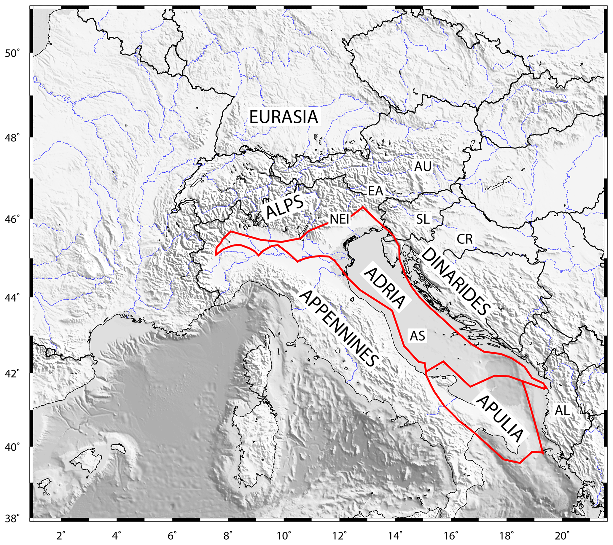
Figure 1 Map of the study area, with topography from ETOPO1 (Amante and Eakins, 2009). Red lines indicate the boundary of the Adria microplate; we refer to the “Adria microplate” as the Adriatic Sea plate domain, also including the Apulia block in the southern Adriatic Sea. Continental lithosphere polygons from the GPlates 2.1 dataset (https://www.earthbyte.org/gplates-2-1-software-and-data-sets/, last access: 12 January 2024) are in agreement with Matthews et al. (2016). AL: Albania; AS: Adriatic Sea; AU: Austria; CR: Croatia; EA: Eastern Alps; NEI: north-eastern Italy; SL: Slovenia.

Notwithstanding the availability of reliable and consistent GNSS solutions at the global scale, such as those provided by the Nevada Geodetic Laboratory (NGL) (http://geodesy.unr.edu/, last access: 12 January 2024; Blewitt et al., 2018), at the regional scale, it may be useful to consider an ad hoc reference framework and to customize the processing scheme in order to obtain high-quality time series and high-quality velocity fields in regions of particular interest. North-eastern Italy (Fig. 1) is a particularly suitable region because of the large number of GNSS stations deployed there by different agencies since the early 2000s to monitor the deformations. North-eastern Italy lies at the northern edge of the Adria microplate, a continental lithosphere block that is part of the distributed deformation zone between the African and Eurasian plates, encompassing the eastern Italian Peninsula from Sicily to the border with Austria and Slovenia as well as the eastern Adriatic coast from Slovenia to Croatia and Albania (Battaglia et al., 2003). The Adria microplate is recognized as having a anti-clockwise motion, implying its collision with Eurasia along its northern tip (Battaglia et al., 2003; D'Agostino et al., 2005, 2008; Serpelloni et al., 2005). The convergence between the Adria and Eurasia plates leads to significant consequences for the deformation of north-eastern Italy, as revealed by the moderate seismicity primarily concentrated in the southern sector of the Eastern Alps and diffused tectonic deformation (Castellarin and Cantelli, 2000; Bressan et al., 2021). Although the deformation rates (2–3 mm yr⁻¹ of N–S shortening; D'Agostino et al., 2005; Weber et al., 2010; Devoti et al., 2011) remain quite low when compared to fast-converging margins like India–Eurasia or Arabia–Eurasia, this is the most seismically active area of the entire Alps chain. Hence, north-eastern Italy is a key region for the understanding of the Adria microplate geodynamics (Brancolini et al., 2019; Magrin and Rossi, 2020). The deformation in the area is currently monitored through GNSS instruments by the National Institute of Oceanography and Applied Geophysics – OGS, the Friuli Venezia Giulia regional council and other entities, providing new and denser data to the information available since the 1960s from the north-eastern Italian subsurface tilt and strainmeter network (Braitenberg and Zadro, 1999; Rossi et al., 2021). The Friuli Venezia Giulia Deformation Network (FReDNet) is the GNSS network established by the OGS to monitor the distribution of the crustal deformation and provide supplementary information for regional earthquake hazard assessment (Zuliani et al., 2018). It currently includes 22 permanent GNSS stations located at distances of 15–20 km from each other in most parts of the region, most of which have been in operation for more than 15 years (more details in Appendix A). FReDNet is part of the OGS seismic and geodetic monitoring system for north-eastern Italy (Sistema di Monitoraggio terrestre dell'Italia Nord Orientale – SMINO), which also includes seismic broadband and short- and mean-period stations as well as strong-motion stations (Bragato et al., 2021, and references therein).

In this paper, we document a dataset of position time series and velocities for 350 stations in north-eastern Italy and surroundings, whose data have been continuously collected over the past 2 decades. The dataset has the potential to provide high-quality and updated information relative to an active but slowly converging margin. Data have been processed, taking advantage of the high-performance computing resources offered by CINECA (https://www.hpc.cineca.it/, last access: 12 January 2024) clusters through the Italian SuperComputing Resource Allocation (ISCRA) initiative and through the resources available inside the HPC Training and Research for Earth Sciences (HPC-TRES) programme co-sponsored by the Minister of Education, University and Research (MIUR). The HPC-TRES training programme, drawn up by OGS and CINECA, is targeted to promote advanced training in the fields of Earth system sciences and to enhance human resources and capacity building through the use of national and European HPC infrastructures and services in the framework of the international infrastructure PRACE – the Partnership for Advanced Computing in Europe (https://prace-ri.eu/, last access: 12 January 2024). In Sects. 2 and 3, we describe the collected input data and the elaboration procedures, respectively. The dataset of time series and velocities is presented in Sect. 4, whereas Sect. 5 illustrates some experiments to evaluate the dataset's quality and robustness. Section 6 provides information on the data availability, and Sect. 7 outlines some final considerations.

2 Input data

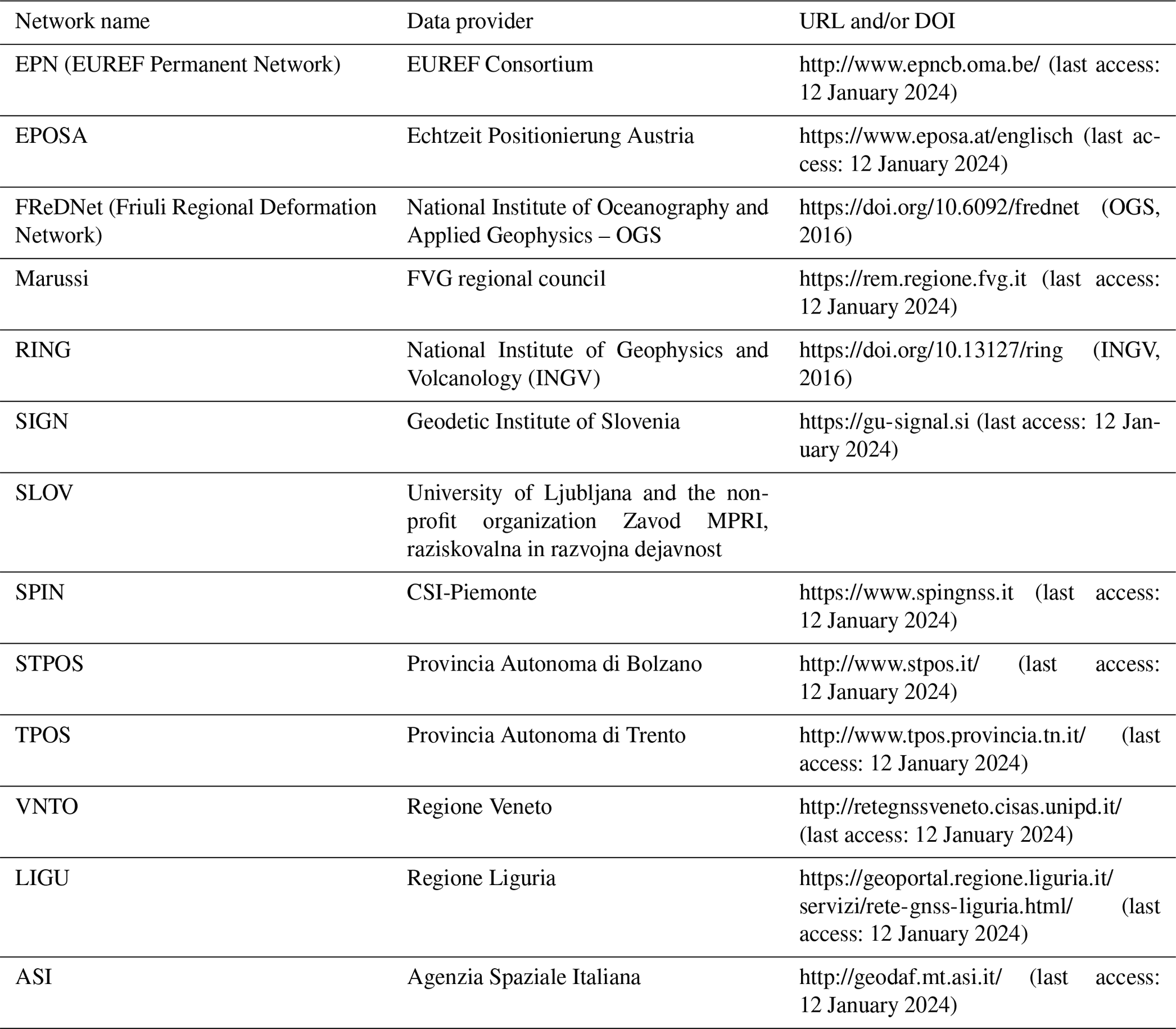
We considered the data recorded by all the available permanent GNSS stations located in north-eastern Italy and surrounding regions (Fig. 2). These stations belong to different networks: the OGS geodetic network FReDNet (http://frednet.crs.ogs.it/, last access: 12 January 2024); the GNSS Antonio Marussi network of the Friuli Venezia Giulia (FVG) regional council (Marussi), with stations located throughout the FVG region that enhance the coverage offered by FReDNet; the Veneto region GPS network (VNTO); the Servizio di Posizionamento SPIN3 GNSS (SPIN), which is a network covering the regions of Lombardy, Piedmont and Valle D'Aosta; the South Tyrolean Positioning Service (STPOS) and the Trentino POsitioning Service (TPOS), which are the geodetic networks of the Autonomous Provinces of Trento and Bolzano, respectively; the Liguria region GNSS network (LIGU); the Rete Nazionale Integrata GNSS (RING) belonging to the National Institute of Geophysics and Volcanology (INGV); the Nuova Rete Fiduciale Nazionale GNSS of the Italian Space Agency (ASI); the European EUREF Permanent Network (EPN), which includes stations managed by different institutions; the Echtzeit Positionierung Austria (EPOSA) network; and the SIGNAL network of the Geodetic Institute of Slovenia (SIGN) as well as other Slovenian GNSS stations acquired by OGS in agreement with the University of Ljubljana and the non-profit organization Zavod MPRI, raziskovalna in razvojna dejavnost (previously with the Slovenian company Harphasea) (SLO_GPS in the following). More details can be found in Appendix B. Although some of these networks were designed for cadastral and civil purposes, the validity of such data for velocity estimates has been demonstrated in several works since the benefit of redundancy and increased spatial density overcomes the noise that is possibly present (Serpelloni et al., 2022, and references therein).

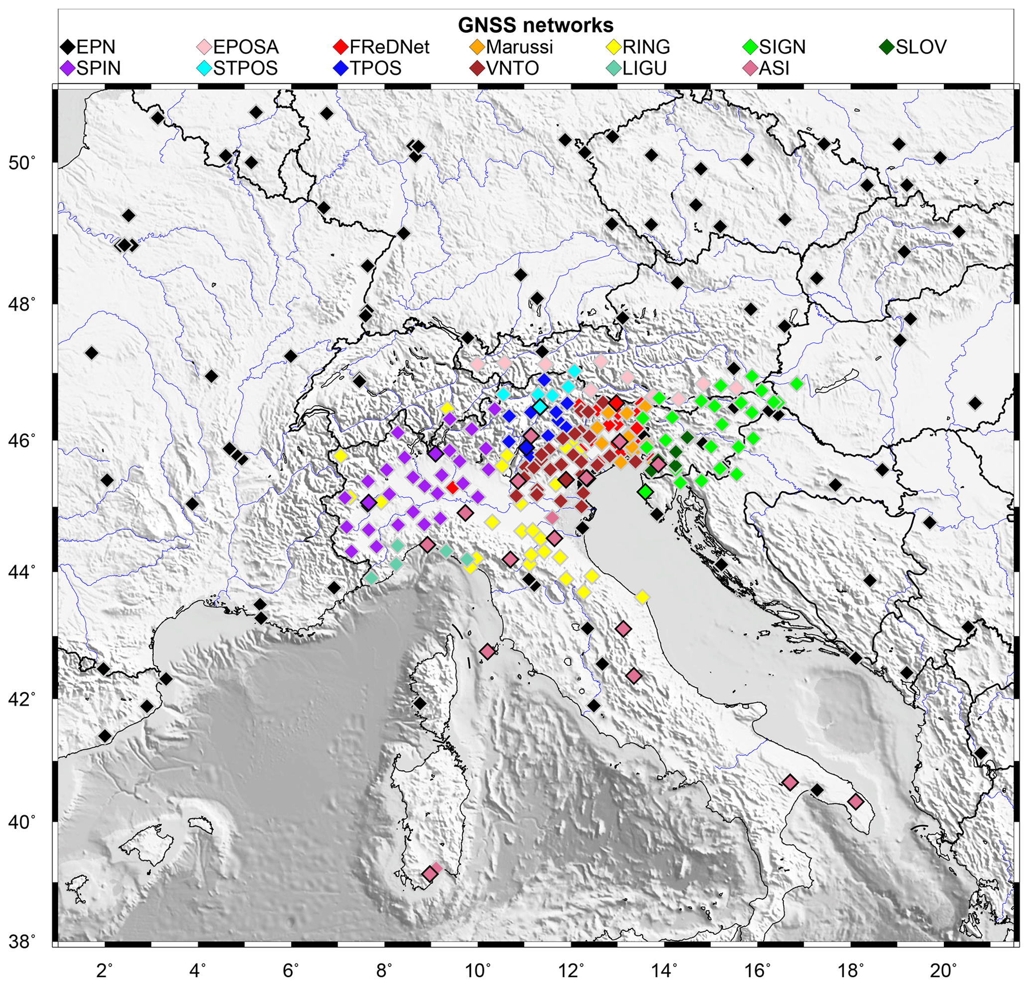
Figure 2 GNSS station locations and associated networks. Different colours stand for different networks, as indicated in the legend (see the main text for the abbreviations). Symbols contoured by black lines indicate those stations belonging to both a regional network and to the European network EPN.

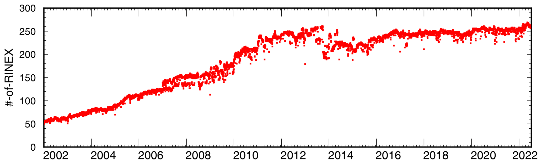
In order to link our solutions to the International Terrestrial Reference Frame ITRF14 (Altamimi et al., 2016), we also consider the data coming from reference sites belonging to the EPN and International GNSS Service (IGS, https://igs.org/data/, last access: 12 January 2024) networks. In a rectangular area extending from 39.75 to 50.70° N latitude and from 1.5 to 21° E longitude and centred in north-eastern Italy, whose size has been empirically selected to obtain a stable position–velocity solution for each of the target stations, we consider as reference sites all the EPN and IGS sites located inside it, with four additional EPN sites located in Sardinia (CAGL, CAG1, CAGZ and UCAG) added to improve the coverage in the southern sector. While our study encompasses more than 350 stations within the designated area (5 stations – GUMM, LECC, LEIB, RUDI and SILL – were moved more than 1 m from the original position; therefore, we renamed them), the actual volume of data is considerably lower. It has shown a progressive increase, starting from just a few tens of data per day in 2002 to reaching approximately 250 data points per day in 2011 (Fig. 3). The drop in the number of stations since 2013 is due to a sudden restriction of the access to several stations located in Slovenia. The data availability depends greatly on station operability, remote connection functioning and decommissioning or installation of stations.

The total number of the daily observation files processed in this study is about 0.57 million.

Figure 3 Number of data available with time.

We have collected GNSS observation data since 1 January 2002. Raw data from the FReDNet network are collected, quality-checked, transformed into Receiver INdependent EXchange (RINEX) format and then released through a public ftp repository as hourly and daily files at both 1 and 30 s sampling. Data from the EPOSA network and SLO_GPS stations are collected in real time through the GNSMART software (Gerhard et al., 2001) and are then converted to RINEX format for post-processing. Finally, RINEX-formatted data deriving from the other networks are collected using different services of data distribution: a public data repository of the networks, EPN data distribution services and the European Plate Observation System (EPOS) service (Fig. 4).

Like the SMINO monitoring system to which it belongs, the FReDNet network aims to provide a monitoring service on a long-term basis. Hence, raw observations and RINEX-formatted data from FReDNet stations are currently continuously retrieved, collected and stored in the OGS internal repository on an hourly and daily basis (https://doi.org/10.6092/frednet, OGS, 2016), where real-time observations are also available. FReDNet data are distributed under a Creative Common License (CC BY 4.0) and are accessible at the link https://doi.org/10.6092/frednet. They are allocated to folders according to the sampling interval and to the date of the acquisition. From the same web page, metadata of FReDNet stations are also retrievable by clicking on the “sitelogs” link.

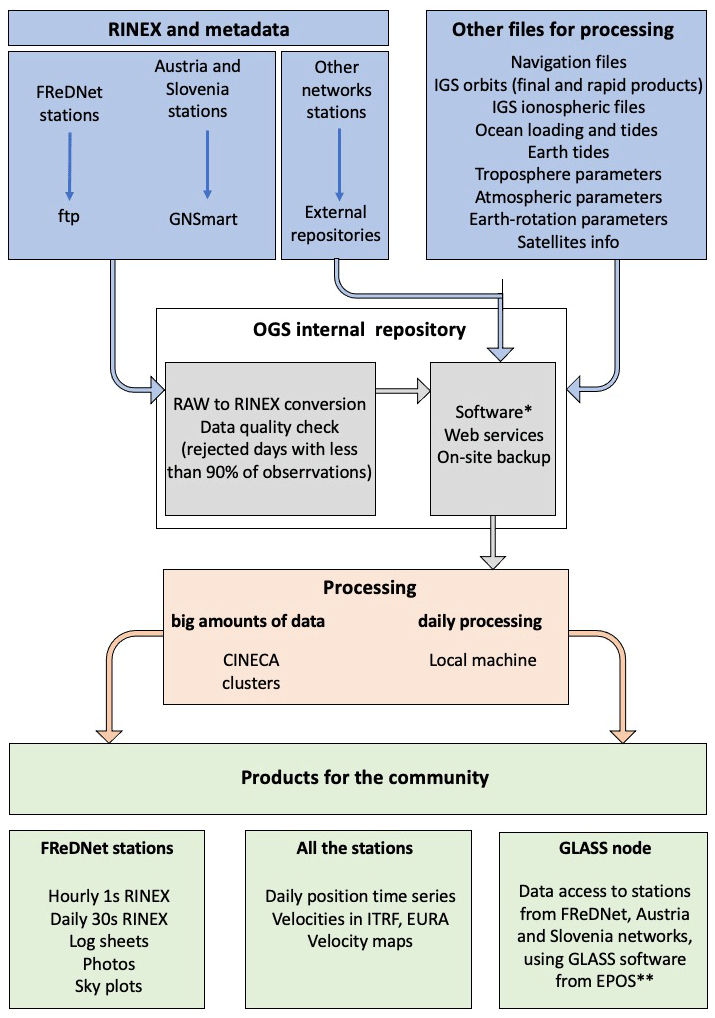
Figure 4 GNSS data flow at the OGS (Italy). * Software used: GAMIT/GLOBK ver10.71 (Herring et al., 2018) for GNSS data processing, GMT ver6.4.0 for plots and maps, GNSMART for downloading raw stream data from Austrian and Slovenian networks and transforming them into RINEX format data, TEQC (Estey and Meertens, 1999) for data quality check (it is end of life, but for GPS data it is still functional), Git ver2.27, a free and open-source system (https://git-scm.com/, last access: 12 January 2024) for script updates and management between different machines, and Anubis ver2.3 (https://gnutsoftware.com/software/anubis, last access: 12 January 2024) for sky plots and RINEX3 generation. ** https://glass.gnss-epos.eu/#/site (last access: 12 January 2024).

Along with the data, site logs containing station metadata (e.g. station location, structure type, terrain description, photos) are collected for each GNSS station. The primary information sources of metadata are the log sheets in IGS format (https://www.igs.org/formats-and-standards/, last access: 12 January 2024) recovered through the public repository of each network and from the Metadata Management and distribution system for Multiple GNSS Networks (M3G) (https://gnss-metadata.eu/site/index, last access: 12 January 2024). If the network does not provide IGS site logs, we extract the information from the RINEX file header. Finally, we verify the compatibility among different sources of metadata, when available.

The metadata describe the history of the equipment, which is useful for classifying discontinuities in the time series. We use this information to populate the list of offsets in the time series for the stations' a priori coordinates. In particular, we define the offsets present in the time series by considering (i) the site-log information on station equipment; (ii) the offsets reported by EUREF and IGS, except those related to changes in the processing procedure; and (iii) the occurrence of earthquakes with magnitudes greater than 5.0 as reported by the ANSS catalogue (U.S.G.S., 2017), with an offset assigned to each station within an empirical radius of influence as a function of the magnitude (using the sh_makeeqdef program inside the GAMIT/GLOBK software, Herring et al., 2018).

Other important information reported in the site log of a GNSS station concerns the structure type and its location (on a building roof, on a building wall or on the ground). The structure for a GPS/GNSS site should be designed to provide stable and secure support to mount the antenna. Therefore, the structure should comply with a certain number of characteristics. The IGS and the University NAVSTAR Consortium (UNAVCO) provide some recommendations for the construction and the installation site (https://files.igs.org/pub/station/general/IGS Site Guidelines July 2015.pdf, last access: 12 January 2024, https://kb.unavco.org/article/unavco-resources-permanent-gps-gnss-stations-634.html, last access: 12 January 2024). It is not always easy to meet all these requirements, because it is difficult to cover all the conditions and because the same environment changes over time, especially near urban areas, due to urban developments. The consequences of non-optimal site conditions are likely to be reflected in data quality, noisy time series and increased uncertainties.

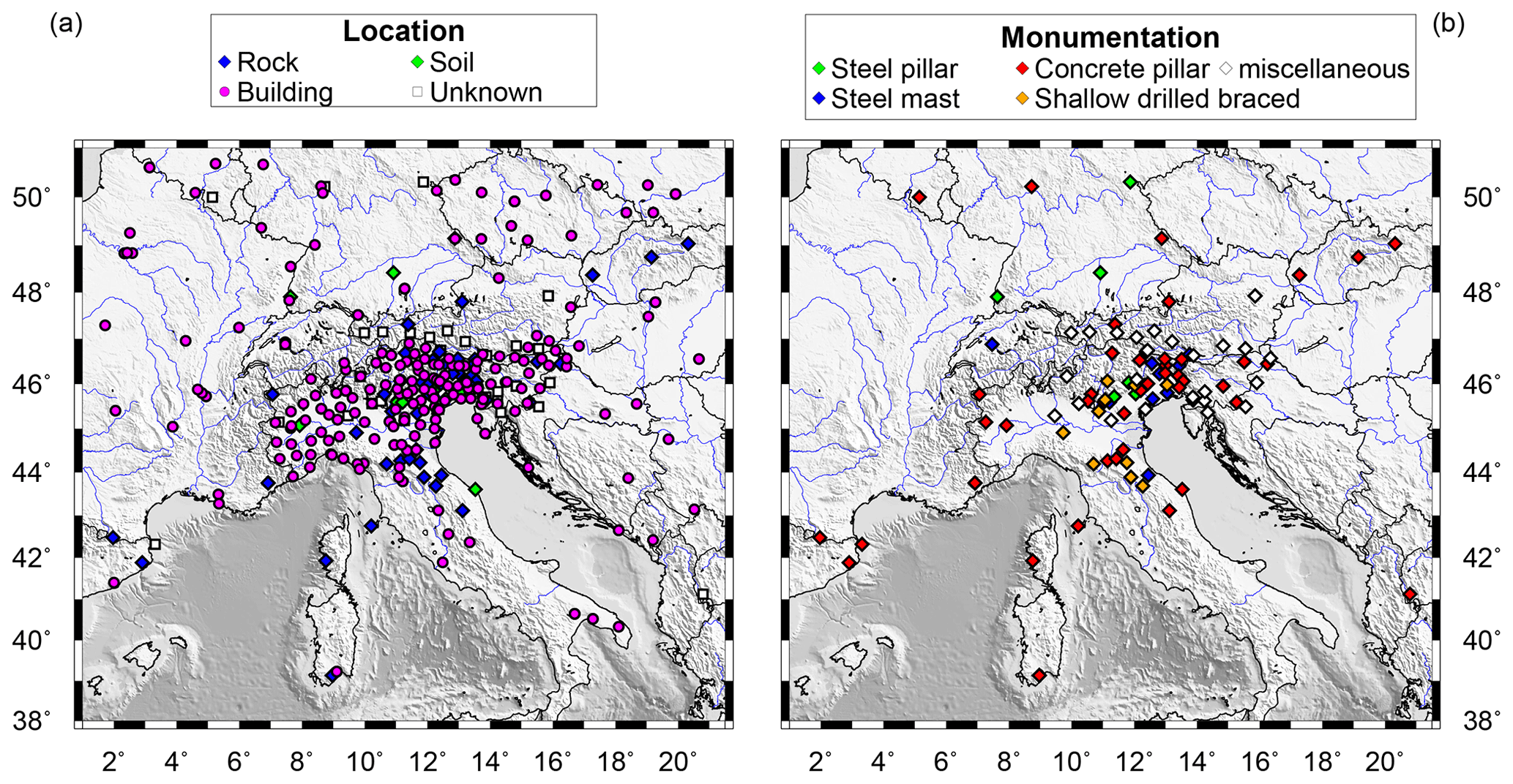
Figure 5 Information on the location and structure type of the GNSS stations considered in this study. (a) Stations classified according to their location. Rock: station installed on hard terrain (not soil) or outcropping rocks. Building: station installed on a building or similar structure, like a wall, both on a roof or fixed to a side wall. Soil: station installed on soft terrain. Unknown: station whose location description is incomplete or ambiguous. (b) Stations not on buildings classified according to structure type. Steel pillar: structure made of a steel column. Steel mast: structure made of a steel bar. Concrete pillar: structure made by a concrete column with or without steel bars inside. Shallow drilled braced: structure consisting of a tripod drilled in the terrain. “Miscellaneous” includes mixed or unspecified material.

The site log of a GNSS site should provide a detailed description of the structure (material type, structure foundation, height and depth of the foundation, geological characteristics of the bedrock, spacing of possible fractures in the bedrock, presence of faults nearby) accompanied by a photograph of the same. However, site logs are often incomplete and lack images. Figure 5 shows the structure information retrieved from the site logs of our stations. Hence, we classify as anonymous those structure locations whose description in the site log is incomplete or ambiguous, and no photos or other sources of information are available to verify the data (Fig. 5a).

For the stations installed on the roof or wall of a building, we can reasonably assume that the stability is more affected by the edifice than by the structure's composition (a steel mast or a concrete pillar). Therefore, we classify only those stations located away from buildings according to the structure material (Fig. 5b).

As can be noticed from the figure, the majority of the stations are located on buildings or walls (251), and just one-third (107) of the stations are located in the free field (10 on soft soil, 57 on exposed rocks and 40 in unknown free-field locations). Approximately 50 % of the latter have concrete pillars as structures (54), ∼10 % have a structure composed of steel rods or a steel tripod (shallow drilled braced, http://ring.gm.ingv.it/?page_id=43, last access: 12 January 2024) (11), while the rest of the stations have steel mast structures (9), steel-pillar-equipped stations (6) or undefined structure types (27).

3 Data processing

We process the GPS data using the GAMIT/GLOBK software package (ver 10.71) (Herring et al., 2018). GAMIT can estimate station positions, atmospheric delays, satellite orbits and Earth orientation parameters (EOPs) from ionosphere-free linear combination of GNSS-phase observables by using the double-differencing technique to eliminate phase biases caused by drifts in the satellite and receiver clock oscillators. It outputs loosely constrained solutions (h files) of the parameter estimates and their covariance matrix. GLOBK is a module which implements the Kalman filtering, and it is used to combine the loosely constrained solutions (between networks and through time) and to constrain the results in a consistent reference framework.

We process the data following these steps:

• definition of the sub-networks (subsets of stations);

• computation of the loosely constrained solutions for each sub-network;

• combination of the sub-network solutions and computation of the daily position for each station;

• computation of the GNSS station velocities.

The RINEX files available each day are processed after being divided into sub-networks to pursue computational efficiency. To do that, we use the netsel program of the GAMIT/GLOBK software package, which considers the geographic distribution of the stations in order to build the sub-networks (see Serpelloni et al., 2022, for a detailed description of the algorithm). Each sub-network is linked to the next one by one station. An additional sub-network that contains two tie sites from each sub-network links all the sub-networks together. We perform some tests to identify the best nominal number of stations for each sub-network, which depends on the number of data available: we select 30 stations and sub-networks until 2008 and 40 stations and sub-networks for the following years. Stations from the SLO_GPS network are equipped with receivers, whose data need to be elaborated using the LC_HELP algorithm of the GAMIT/GLOBK software, which uses ionospheric constraints. To include these stations in the solution, we process them in a separate sub-network along with some tie sites (TRIE, GSR1 and KDA2). The tie sites of this sub-network will be excluded from the netsel site list and will be added to the tie site sub-network afterwards.

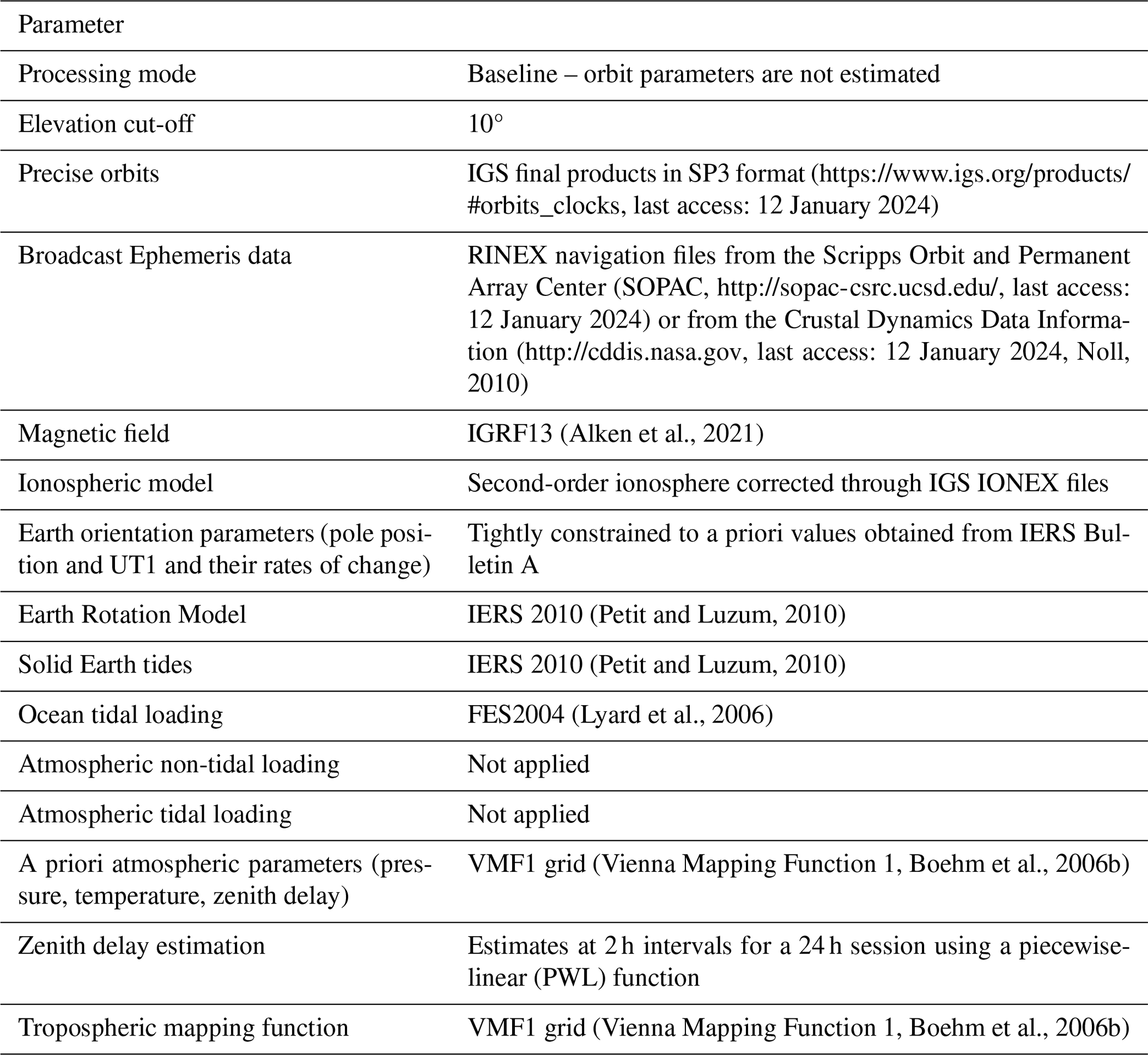
We compute the loosely constrained solutions using the GAMIT module. GPS phase data are weighted according to an elevation-angle-dependent error model (Herring et al., 2018) using an iterative analysis procedure whereby the elevation dependence is determined by the observed scatter of phase residuals. Satellite precise orbits are retrieved from the IGS repository (http://www.igs.org/products/, last access: 12 January 2024, Johnston et al., 2017). The first-order ionospheric delay is eliminated by using the ionosphere-free linear combination for all the stations except the SLO_GPS ones. Further details about the models and parameters are reported in Table 1.

Table 1 GAMIT solution parameters.

To obtain the position time series, we use the GLOBK module to combine the daily loosely constrained solutions of the sub-networks in a single daily solution, leaving the constraints free. Since we want to express the solutions in the International Terrestrial Reference Frame (ITRF14/IGS14 by Altamimi et al., 2016; in particular, we use the newer GNSS geodetic reference framework IGb14), we then apply generalized constraints (Dong et al., 1998) using the glorg program. For this purpose, we use a six-parameter Helmert transformation (translation and rotation) estimated by minimizing the difference in the positions of a set of stations with well-defined coordinates and velocities (reference sites) as a priori coordinates. We do not explicitly use a scale to avoid potential absorption of height signals, following Herring et al. (2016). The results are daily position estimates for each station, consistent with the IGb14 reference framework.

The time series are visually inspected to identify offsets that are not due to equipment changes or earthquakes. We automatically remove outliers using two criteria similar to those used by Floyd et al. (2010). First, we remove the daily positions that have formal uncertainties greater than 20 mm. Then we fit the time series to a model consisting of a linear trend and offsets through a weighted linear regression by using the tsfit program. The positions with residuals greater than 3 times the weighted root-mean-square (rms) value of the fit are also removed. Finally, by applying the real_sigma algorithm (Floyd and Herring, 2019), which allows us to account for temporal correlations in the data, we estimate random walk values for each station from the analysis of the outlier-adjusted time series and identify specific sites exhibiting a random walk noise level exceeding the 2.0 mm² yr⁻¹ level, which are also removed.

To compute the velocity field, we use the forward-running Kalman filter implemented in the GLOBK module, in which the state vector includes the positions and velocities for each station (Herring et al., 2016). The input data are the daily loosely constrained solutions, as they may be freely rotated and translated, thus eliminating the need to include EOP in the state vector and their full variance–covariance matrices. Following Herring et al. (2016), from the analysis of the previously generated time series, we retrieve the list of outliers to be excluded from the computation and the site-specific parameters to model the stochastic noise in the station positions. In each epoch, the Kalman filter updates positions and velocities. With the aim of reducing the computation time, we divide the stations into sub-networks using netsel. We use a nominal number of 90 stations for each sub-network and the noise model obtained from the time series analysis. First, we estimated the velocities and positions of the stations included in each sub-network. Then, we combine the solutions obtained for each sub-network in a single solution. At the end of the forward Kalman filter run, we align positions and velocities to the IGb14 reference framework using a 12-parameter Helmert transformation (rotation, translation and their rates). Velocities of stations within 1 km distance (including differently named stations at the same location) are equated in this reference framework realization. Finally, we recalculate the time series and velocities using the values obtained in the previous iteration as a priori coordinates and expand the list of reference stations to include all the stations with random walk values lower than 0.5 mm² yr⁻¹. As reported by Herring et al. (2018), the time series that best represent the final velocity solution are those computed considering all stations in the solution to be reference sites. We also express our solutions relative to the Eurasia plate as defined by the Altamimi et al. (2017) plate motion model (ETRF14 reference framework) using the same procedure adopted for IGb14.

Computing infrastructure

Modern computational infrastructures allow the analysis of huge amounts of data with extraordinary advantages in terms of operational cost for data storage, processing and time saving, leading to the timely provision of homogeneous products. We exploited the CINECA (https://www.hpc.cineca.it/, last access: 12 January 2024) high-performance computing (HPC) resources to process and analyse in a very short time all the GNSS data available in the study area between 1 January 2002 and 30 June 2022. We used the GALILEO100 cluster, which is equipped with 554 compute nodes with a 2× CPU Intel CascadeLake 8260 with 24 cores, 2.4 GHz and 384 GB RAM DDR4. The job scheduling and workload management system is SLURM 21.08 (https://wiki.fysik.dtu.dk/niflheim/SLURM, last access: 12 January 2024). SLURM is designed to accomplish three key functions: (i) allocation of exclusive or non-exclusive access to computing nodes to users for a specific duration of time; (ii) provision of a framework for managing the work (starting, execution and monitoring) on the set of allocated nodes; and (iii) resource distribution handling by managing a queue of pending jobs.

Figure 6 is intended to give an indication of the performance of CINECA clusters for GNSS data elaborations showing the computation time on GALILEO100 computing nodes to obtain the GAMIT solutions as a function of the number of stations considered on each job sent to the compute nodes. The figure shows that the computation time varies on average with the square of the number of stations. Although the calculations of the GAMIT solutions are the most time-consuming jobs of the processing procedure, the total computation time on GALILEO100 depends not only on the number of available daily data, but also on the adopted parallelization strategy (i.e. the number of jobs sent to resources on compute nodes) and the occupancy of the machine (i.e. queue waiting time). In our study, we managed to process 2 decades of GNSS data in 1 week. We implemented the same procedure described in the previous section on a local machine to process the data daily following 30 June 2022, with the aim of keeping the products updated. The daily processing is automated by using the crontab utility. More details on the implementation on the local machine can be found in Appendix C.

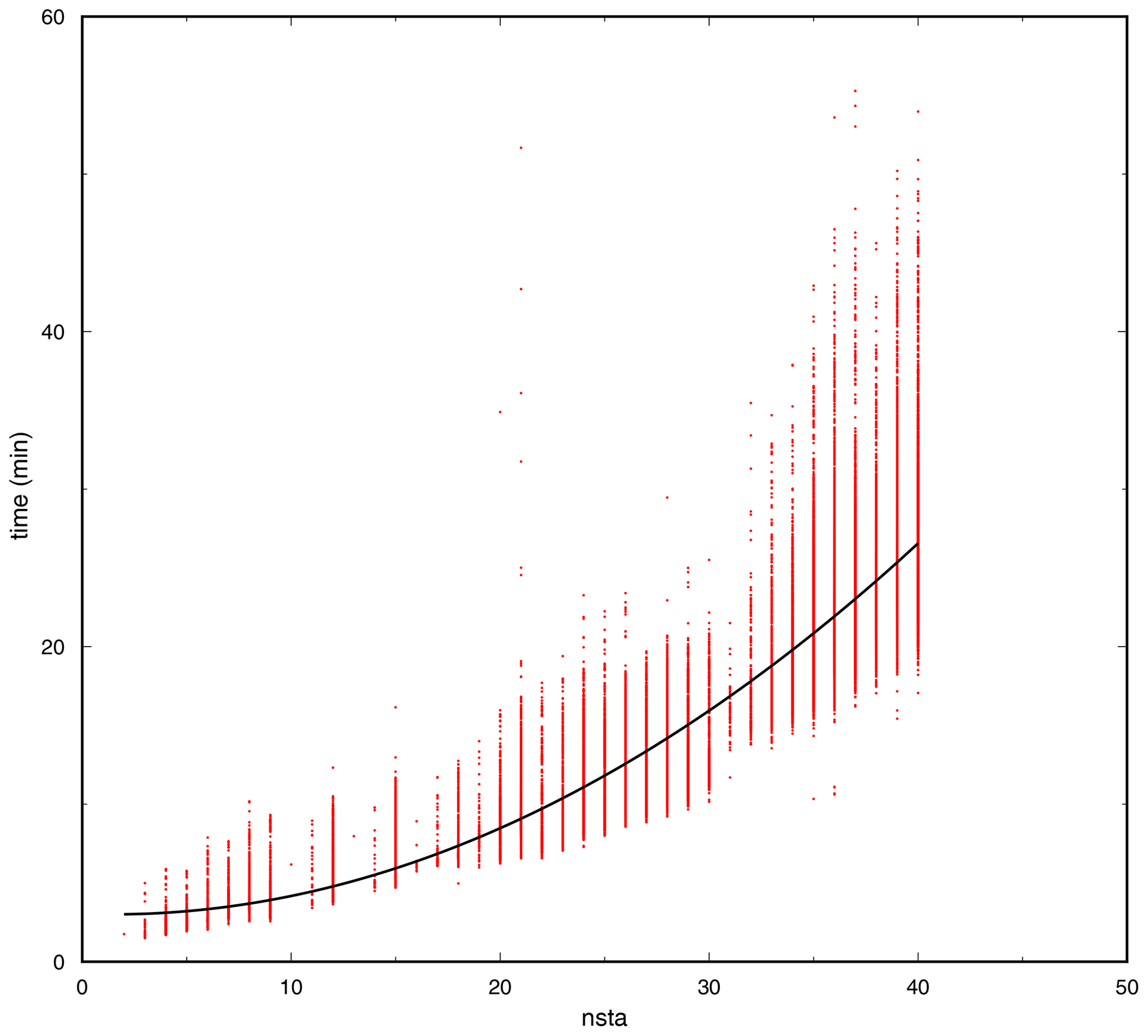
Figure 6 Calculation time for GAMIT solutions using the GALILEO100 cluster as a function of the number of sites (nsta).

4 Geodetic time series and velocity dataset

This section considers the geodetic time series and velocity products provided. In support of the dataset, we illustrate several tests performed to check the reliability of the documented results. For the sake of simplicity, we define the results of this study as “final time series” and “final velocities” and those estimations retrieved from the tests as “test time series” or “test velocities”.

4.1 Time series quality

We illustrate here the GNSS time series resulting from the data processing as a whole, whereas time series for single stations are provided in the dataset, as explained above.

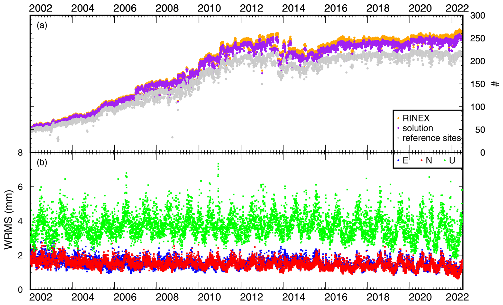
Figure 7 (a) Evolution of RINEX data available with time (orange dots), stations included in the solutions (purple dots) and stations used in the reference framework realization (grey dots). (b) Weighted root-mean-square (WRMS) scatter of the fits to the coordinates of the reference framework stations in the northern (red), eastern (blue) and upward (green) components.

The time series length and quality depend on the number of good observations recorded at the sites, which is reflected in the number of solutions obtained for each station. Figure 7 shows the evolution of RINEX available with time, the sites included in the solution and those being used in the reference framework realization, along with the weighted root-mean square (WRMS) of the fits to reference framework stations. Through data processing, the recorded RINEX allowed almost 97.1 % of the solutions (purple dots in Fig. 7a) to be obtained, a percentage which is indicative of the goodness of the dataset and of the adoption of an appropriate processing strategy. The percentages of missing solutions (∼3 %) are likely due to incomplete data records (RINEX with fewer than 864 daily observations, i.e. with less than 30 % of registrable daily observations) or bad data. As illustrated in Sect. 3, in order to stabilize the solution, we consider all stations with a random walk value lower than 0.5 mm² yr⁻¹, which led us to consider as reference stations ∼80 % of the available stations after 2011 and even ∼90 % or more in the first decade (grey dots in Fig. 7a). The average WRMS fit to the reference framework stations (Fig. 7b) is 1.7, 1.8 and 4.2 mm in the northern, eastern and upward components, improving up to 20 % in the latter since 2011, possibly thanks to the equipment improvements.

Figure 8 shows the stations' noise level through the representation of the WRMS of the time series and the rms of the phase residuals. Notably, 90 % of the stations show low noise levels, with values below 2 mm in the horizontal components and below 4.1 mm in the vertical one.

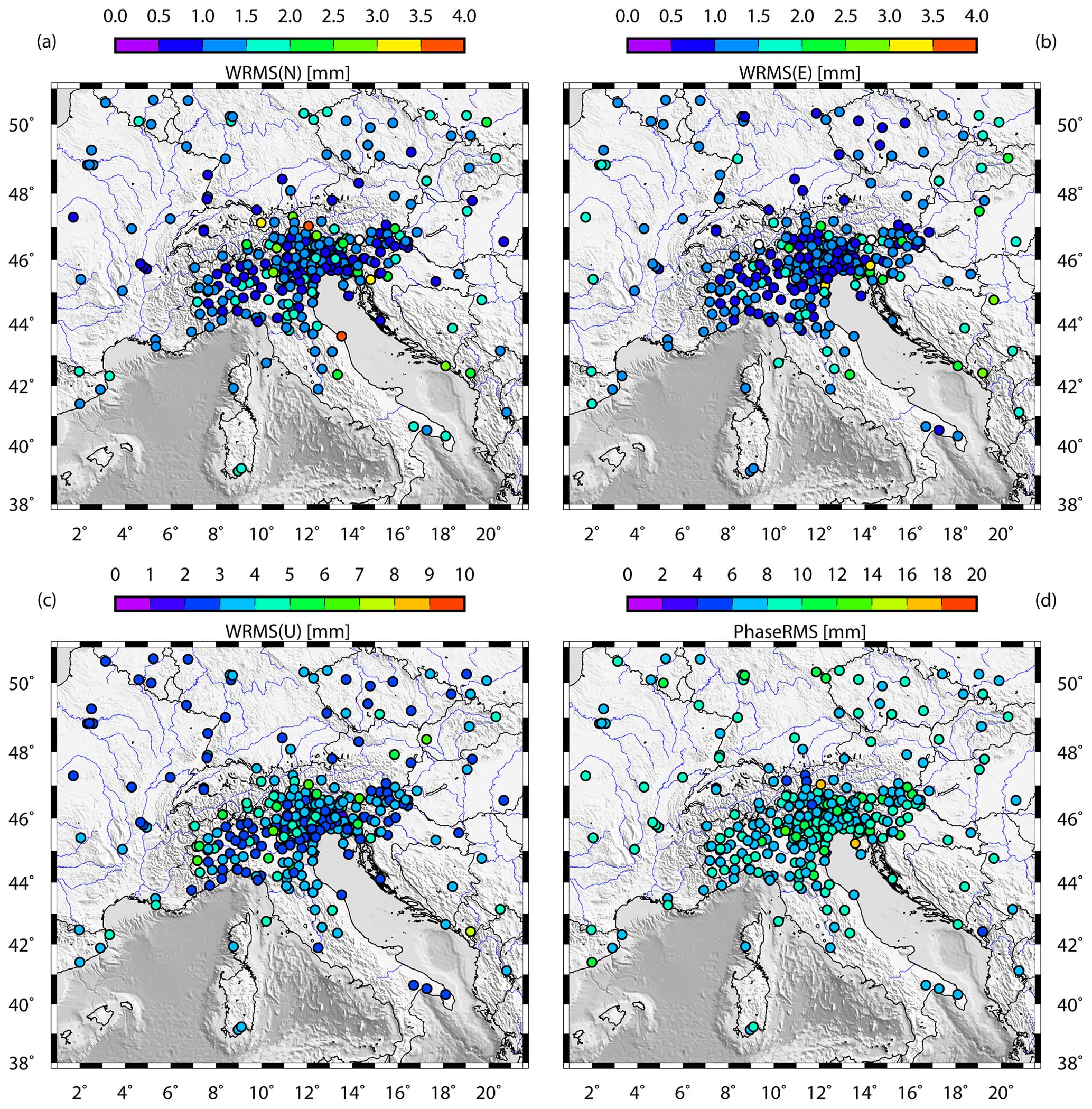
Figure 8 Time series WRMS in the horizontal (a, b) and vertical components (c) and time series rms of the phase residuals (d).

4.2 Geodetic velocities

The length of the time series is generally considered fundamental in determining the accuracy and precision of the estimated linear velocities. Blewitt and Lavallee (2002) show that a coordinate time series of 2.5 years is the minimum range to reduce velocity errors due to annual time series signals, caused primarily by surface loading due to hydrology and atmospheric pressure. However, the authors recommend using time series longer than 4.5 years to almost completely eliminate velocity biases. Data over a period less than 4.5 years are not suitable for studies requiring an accuracy of less than 1 mm yr⁻¹, and the best results are obtained by using long time series (>8 years in length), which allow velocities to be estimated with accuracies of 0.2 mm yr⁻¹ in the horizontal component and 0.5 mm yr⁻¹ in the vertical component (Masson et al., 2019).

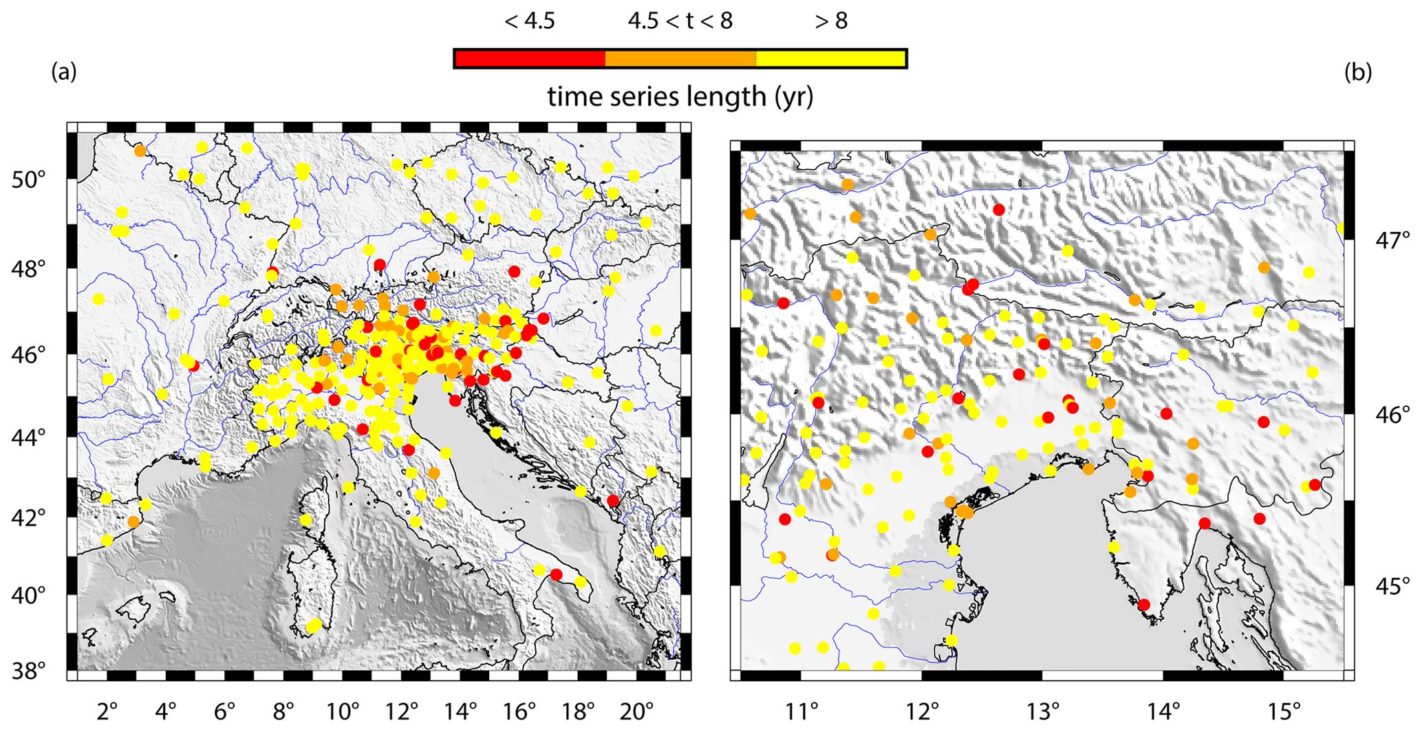
Figure 9 Time series length of the stations considered in this study (a) with a zoom on north-eastern Italy (b).

The stations considered in our study provide time series spanning from 0.27 (HELM) years to 20.49 years (among others, we cite AQUI, GENO, GRAZ, GSR1 and TORI), as shown in Fig. 9. Most of the sites provide time series longer than 4.5 years (84.4 %) and even longer than 8 years (69.4 %), whereas just a small percentage are new stations providing coordinate time series shorter than 1 year (8.9 %). However, newer stations are often located in the vicinity of older stations, thus also allowing the retrieval of reliable and stable results for that particular area (see Fig. 9b).

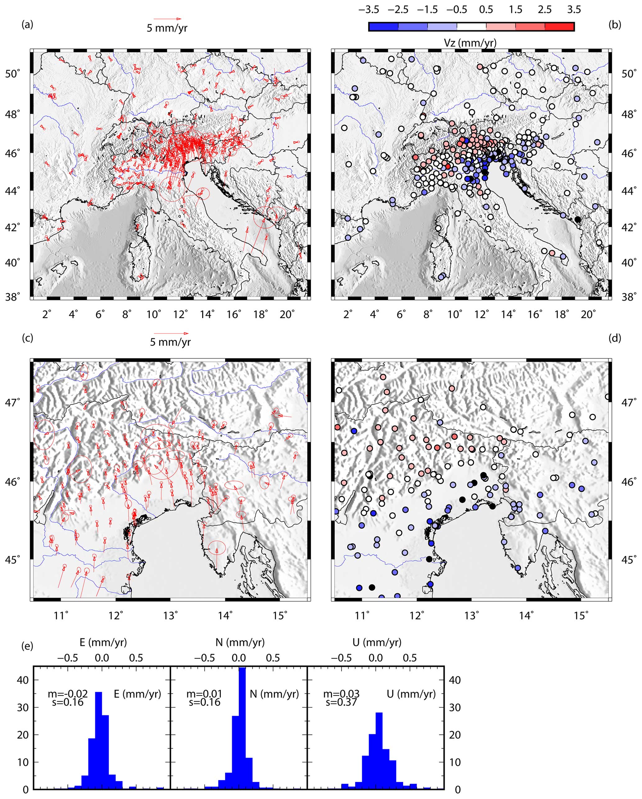
Figure 10 Estimated velocities with 95 % confidence error ellipses in the horizontal (a, c) and vertical components (v_z) (b, d). (e) Histograms indicating the differences, along the three components, between velocity estimates calculated with GLOBK using the procedure described in the data processing section and those calculated using tsfit considering the stations with minimum 4.5-year long time series. Overall, the differences have a Gaussian shape, with mean and standard deviation values firmly below 1 mm yr⁻¹.

We estimated the velocities and uncertainties of all the stations for the horizontal (Fig. 10a, c) and vertical components (Fig. 10b, d) using the GLOBK software. For completeness, we have also calculated the velocities using tsfit, a program that provides a linear fit of the time series, and we have compared the results (Fig. 10e), finding sub-millimetre differences. The estimated velocities in ETRF14 show the active deformation on the Adriatic side of the central Apennines at the few stations located in south-eastern Italy (Apulia region) and in north-eastern Italy, with horizontal displacement directed to the north-east with values of 2–3 mm yr⁻¹ in the Apennines and also on the Friulian plain and coast. The north-eastern Italian Alps, instead, move at slower rates around 1 mm yr⁻¹. Significant horizontal motion is estimated in south-eastern Italy, especially in the northern velocity component, with 3.8 and 4.2 mm yr⁻¹ at the USAL and MATE stations, respectively. The fastest motion (∼7 mm yr⁻¹) is estimated at the TARS and FATA stations (located close to each other and indistinguishable at the scale of Fig. 10). However, this value is not reliable because these stations provide less than 1 year of observations, as can be inferred from the high uncertainty. The estimated vertical displacement highlights the subsidence in the Po Basin (up to 3.5 mm yr⁻¹) and the uplift in the mountains, which is more accentuated in the Eastern Alps than in the Apennines. In addition to the European reference sites located beyond the Italian territory, the stations in north-western Italy also show no significant displacement. The single exception is the LODI station, whose anomalous behaviour (∼2 mm yr⁻¹ velocity in the horizontal components and ∼2.8 mm yr⁻¹ uplift) is due to its location on the top of a depleted methane reservoir recently converted to an underground gas storage facility (Guidarelli et al., 2022). Zooming into the north-east of the study area (Fig. 10c), a pattern of south–north decreasing velocities is distinguishable from the Friulian coastline and plain to the southern sector of the Eastern Alps with an NNW orientation, whereas the stations located in Slovenia and Croatia show NNE-oriented velocities. An anomalous south-directed motion is estimated in the OCHS station in the Eastern Alps, likely due to a landslide motion occurring along the slope where the GNSS station is located.

5 Evaluation of the quality and robustness of the dataset

To evaluate the quality and robustness of the dataset, we perform some experiments with the processing procedure, analysed the quality of the stations and compared our findings with previous studies.

5.1 Data processing tests

After determining the time series, velocities and positions for each station, we test their stability and the reliability of the adopted processing procedure. For that, we perform a number of experiments on the available dataset to check for potential effects of selected options of the data processing with GAMIT/GLOBK (i.e. considering or avoiding tidal or non-tidal loadings or changing the reference stations) on the results. In this way, if these tests do not highlight significant differences with the study results illustrated in the above sections, we can reasonably conclude that our results are reliable and are not biased by processing errors.

In one test, we change the model used to estimate the atmospheric delay. Instead of using the default Vienna Mapping Function numerical weather model (VMF1) calculated by TU Vienna by interpolating hydrostatic and wet mapping function coefficients as a function of time and location (Boehm et al., 2006b), we adopt the Global Mapping Function (GMF) model developed by Boehm et al. (2006a) which fits the European Centre for Medium-Range Weather Forecasts (ECMWF) data over 20 years. Then, since tides and non-tidal loadings are primary sources of time-variable displacements in station coordinates, we perform a test in which we consider the non-tidal atmospheric loading in the processing using a global gridded dataset provided by MIT. For both tests, we recalculate the time series and compare them to the original solution, finding no significant dissimilarity with differences below 1 mm, in agreement with previous studies (Steigenberger et al., 2009; Labib et al., 2019).

Regarding the position time series and velocity estimations, we recall here that one delicate step in the procedure is knowing how to perform editing and weighting of the data as well as the realization of the reference framework. To test these issues, we need to consider which stations to include explicitly, how to treat the orbits and the EOP, as well as practical constraints on computation speed and data storage. Although the GPS satellites provide a natural dynamic framework for ground-based geodesy, the doubly-differenced phase observations do not tie a ground station to the orbital constellation at the millimetre level. We define and realize a precise terrestrial reference framework by applying constraints to one or more sites in our network. To do that, we use the generalized constraint method of glorg, in which up to 14 Helmert parameters (three translations, three rotations, one scale and their rates) are estimated such that adjustments to a priori values of the coordinates of a group of stations are minimized. For continental-scale networks like the one considered in this study, we estimate translation and rotation and include as reference sites a set of distributed stations for which we have good a priori values and sound data.

Hence, we perform some tests to check the goodness of the stabilization framework considered. We recalculate the time series by applying the translation-only transformation as in the EUREF standards (https://www.epncb.oma.be/_productsservices/analysiscentres/combsolframe.php, last access: 12 January 2024) and find negligible differences in the time series. We then perform some tests for the first step of velocity estimation. First, we use as reference sites two different subsets of the reference site set used in the final processing (see Test-1 and Test-2 in Fig. D1 in Appendix D). Second, in the second step of velocity estimation, we consider a regular grid of reference sites generated considering a site every 2° (∼222 km) (see Test-3 in Fig. D1 in Appendix D). Finally, we calculate the velocity field in our study area for each test. Overall, the mean difference values with respect to final velocities are very small, i.e. up to 0.02 mm yr⁻¹ in the north, up to 0.06 mm yr⁻¹ in the east and up to 0.14 mm yr⁻¹ in the vertical component.

Finally, we perform two final experiments to evaluate the effects on the velocity results of introducing the periodic term (annual signal) in the coordinate time series fitting and applying a less restrictive criterion for outliers, i.e. 5 sigmas instead of 3 sigmas. The mean differences, with respect to the final velocities, are of the order of 0.02–0.03 mm yr⁻¹ in both cases for stations with at least 4.5 years of time series length.

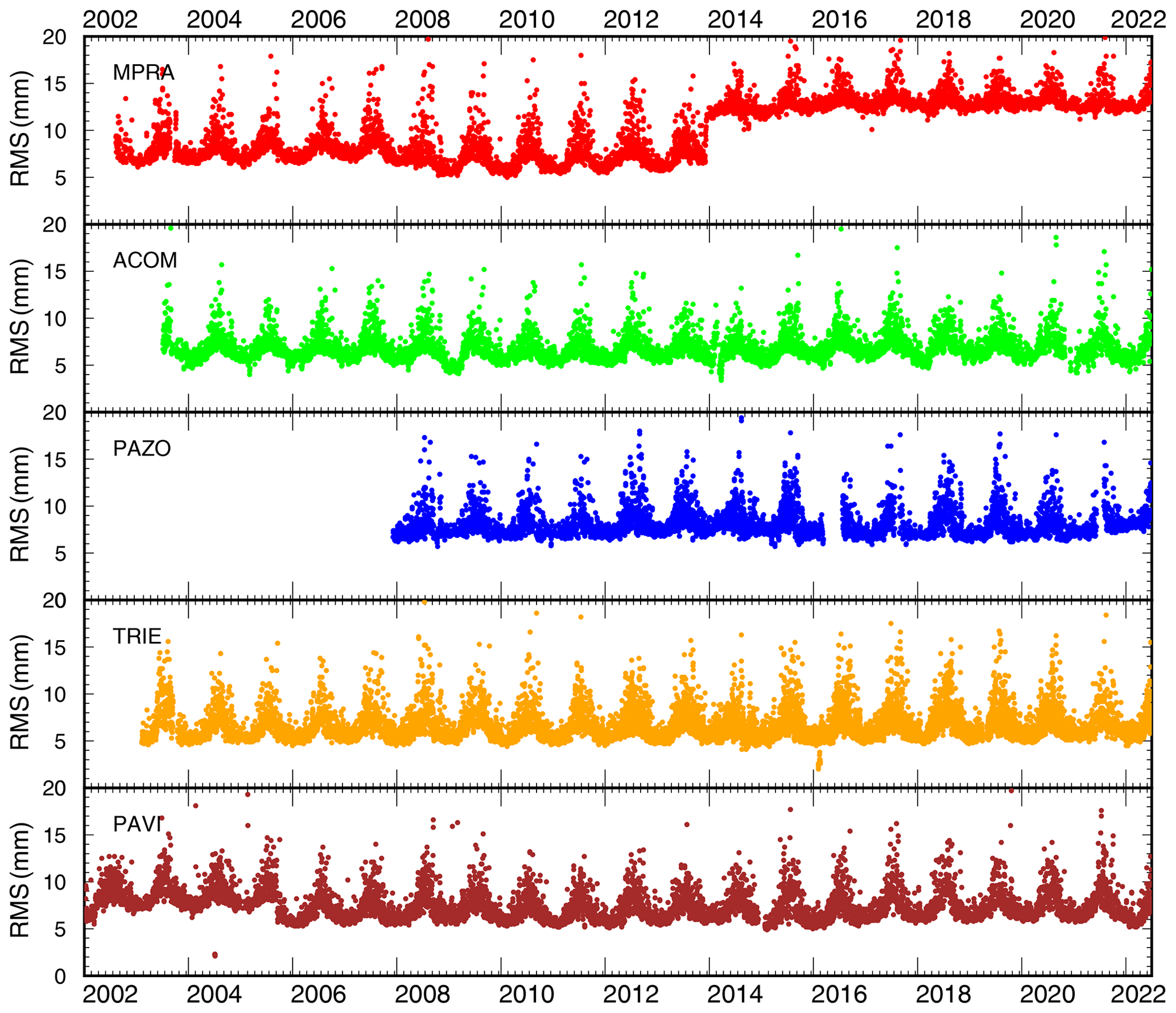
Figure 11 Variation of the rms of the phase residuals with the times of the different GNSS stations.

5.2 Considerations of the station quality

The alteration of the environmental conditions surrounding a GNSS station affects the rms of the phase residuals. The environmental changes can be related not only to climatic conditions, e.g. an increase in the number of weather perturbations due to the climate change, but also to urban developments in the proximity of the stations, building, vegetation growth, radio-electronic source perturbations or traffic increase. In Fig. 11 we plot the rms variation with time for some stations. A seasonal increase in the rms is visible everywhere throughout the considered time interval.

The phase rms, typically 4–7 mm, increases to 15–20 mm in July–August. This characteristic holds true for any station, whether it is located near the coast (i.e. TRIE), in the middle of the plain (e.g. PAZO or PAVI) or in a mountain context (i.e. ACOM, located at 1774 m altitude; MPRA, located at 808 m altitude; ZOUF, located at 1946 m altitude). The same also occurs at the stations in northern Europe; thus, it is a characteristic independent of the geographic setting. A cross-check on the sky plots shows that the phase rms increases particularly during the daytime. We suspect that this is due to incorrect modelling of the atmospheric delay. We certainly know that data coming from sites in the tropics are characterized by higher-phase noise due to the higher water vapour content of the atmosphere. Orographic features such as mountain ranges are prone to producing a highly turbulent and asymmetric atmosphere, which is particularly challenging to model. In other words, tropospheric asymmetries associated with topography, such as being on a mountain range's windward or leeward side, can produce asymmetrical time series scatter due to local-scale weather conditions (Materna, 2014).

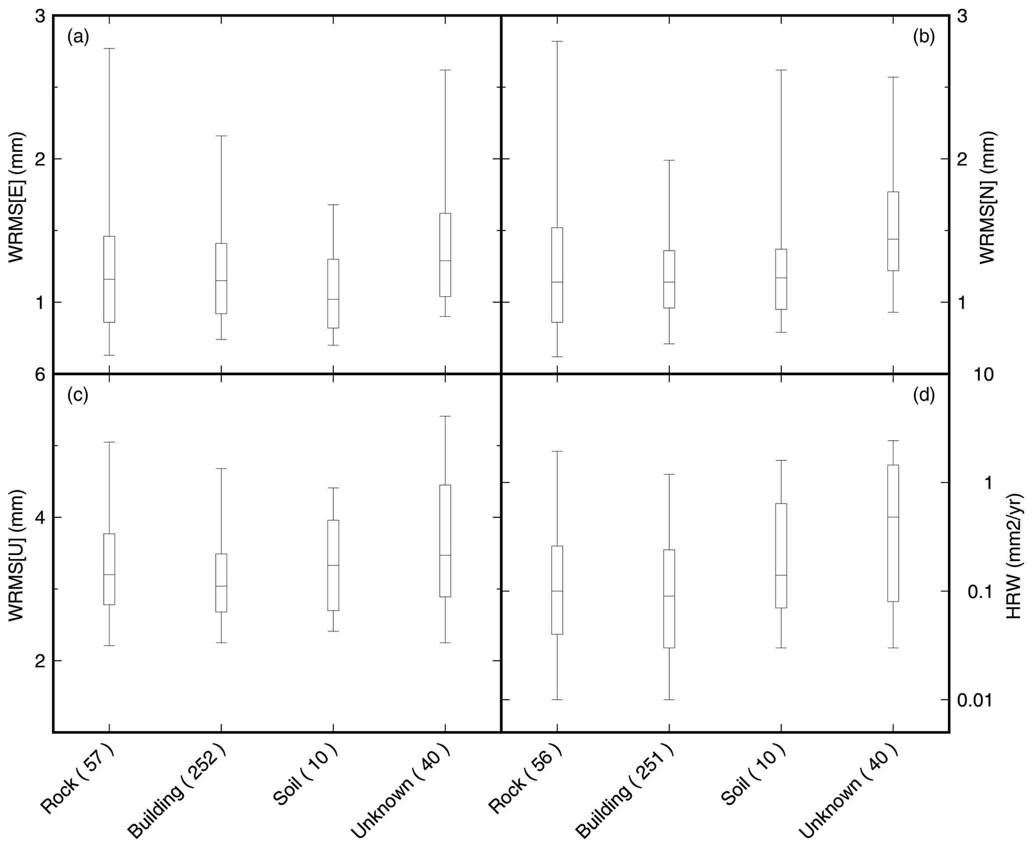
Figure 12 Box-and-whisker plots showing the distribution of the WRMS values estimated from the scatter of the station time series residuals along the eastern (a), northern (b) and upward (c) components, and the equivalent horizontal random walk (HRW) represents the time-correlated noise. The line in the centre of the box is the median value, the boxes encompass 50 % of the stations (25th to 75th percentiles) and the whiskers encompass 90 % of the stations (5th to 95th percentiles).

Further considerations should be made for the MPRA station, which shows a systematic increase in the phase rms since 2014. This condition is due to the construction of an electric tower in the vicinity of the station, which has perturbed the site's noise level, leading to increased uncertainties evident in the station time series (see Appendix A). Also, the PAVI station exhibits a systematically different rms of the phase residuals since the second half of 2005, showing a decrease of ∼2 mm. This decrease is likely due to a change in the equipment. The Trimble Zephyr Geodetic antenna (TRM41249.00) on 14 September 2005 was substituted by a Leica choke ring antenna (LEIAT504) which features superior multipath rejection with uncompromised phase centre stability (<1 mm) and is resistant to RF jamming (http://uec-sigmat.com/Leica AT504 (GG) Choke Ring Antenna - gps_gnss.html#productCollateralTabs1, last access: 12 January 2024). However, the phase rms decrease is not of such a magnitude so as to be noticeable at the uncertainty level or evident in the position time series of the site (see the PAVI time series in the dataset).

Many authors have investigated the contribution of geodetic structure to GNSS time series noise properties (e.g. Herring et al., 2016; Langbein and Svarc, 2019, and references therein). However, our dataset mainly comprises stations installed on buildings, and each class of free-field installation (as defined in Fig. 5) consists of a limited number of stations. Therefore, inferring reliable conclusions about the different free-field installation types is impossible. In Fig. 12, we compared the noise properties of the time series (WRMS of the three components and horizontal random walk – HRW) of stations installed on buildings with those of free-field installations. We conclude that the stations on buildings are not significantly different from the stations installed on outcropping rocks.

5.3 Comparison with previous works

Different research groups published estimations of the velocity field in the area of interest of this study. Since the processing software or user-selected options can vary between different authors, through the comparison of our estimated velocities with those calculated by other researchers, we can evaluate the reliability of our solutions. If the misfits are not significant, we can infer that our results are independent of data treatment and that our solutions are robust. By contrast, if resulting velocities are inconsistent between different studies, this can likely be ascribable to the differences in the data treatment performed. It would be complicated to discriminate which research group has provided the best estimate of the velocity field.

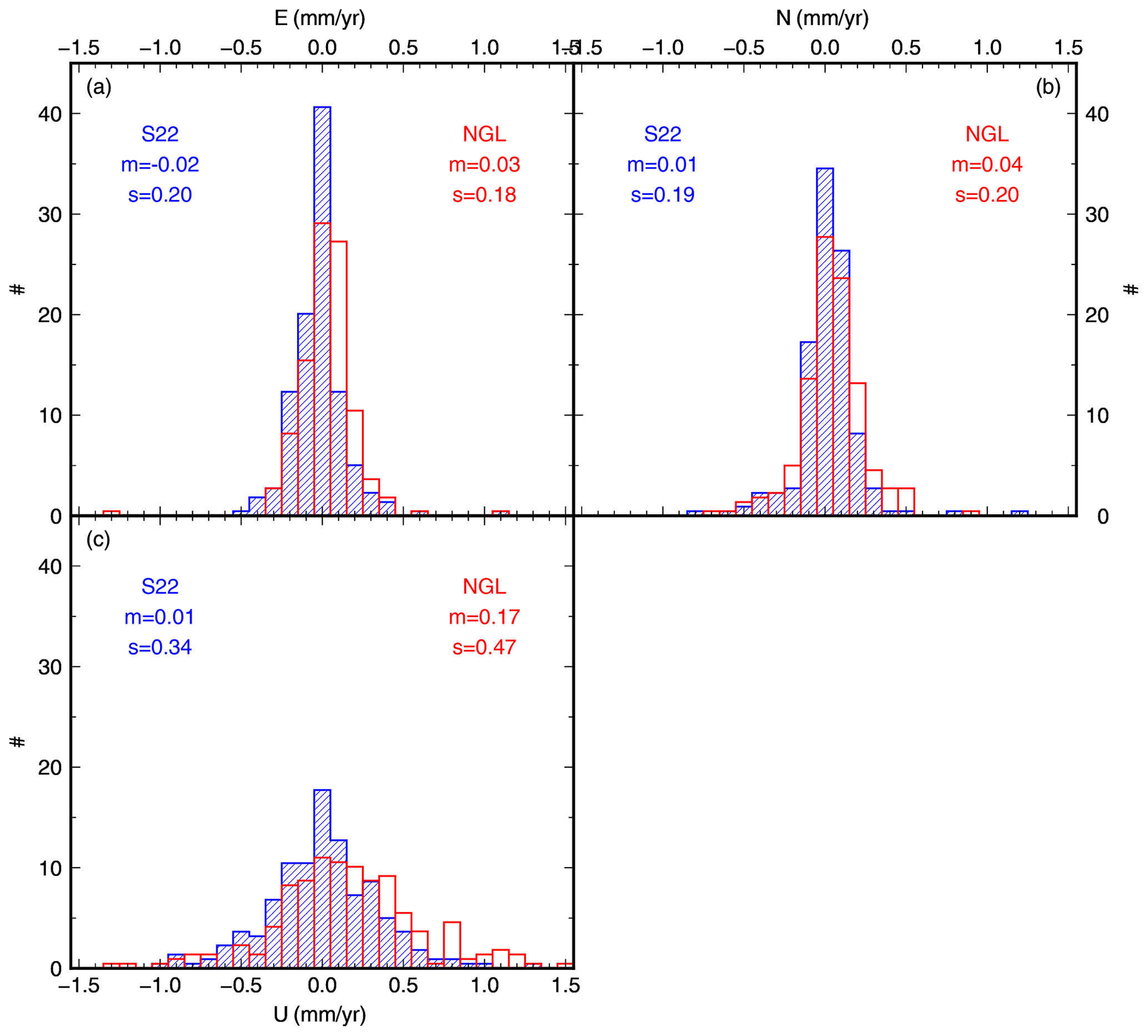
Figure 13 Histograms of the differences between the velocity values estimated in this study, along the three components, and those estimated by Serpelloni et al. (2022) (S22, solution in blue colour) and by the Nevada Geodetic Laboratory (NGL, solution in red colour). Only the stations with a minimum of 4.5 years have been taken into consideration for the histograms.

We compared our results with those calculated by the NGL, downloaded in the IGS14 reference framework from http://geodesy.unr.edu/ on 3 March 2023, and by Serpelloni and co-workers, who recently published the surface velocity of the Euro-Mediterranean region (Serpelloni et al., 2022). The NGL uses the MIDAS software (Blewitt et al., 2016) to estimate the velocity field and automatically estimate the time series trend, identifying step discontinuities, outliers, seasonality and skewness in the data. Serpelloni and co-workers use the code of the Quasi Observation Combination Analysis (QOCA) software developed by the JPL (https://qoca.jpl.nasa.gov, last access: 12 January 2024) to analyse the time series and estimate the linear velocities. The comparison results are shown in Fig. 13 as histograms of solution differences. Overall, the mean differences are negligible, ranging from 0.01 to 0.04 mm yr⁻¹ in the horizontal components and from 0.01 to 0.17 mm yr⁻¹ in the vertical one, with the standard deviation ranging from 0.18 to 0.47 mm yr⁻¹. Slightly greater values are found in the comparison with the NGL solution, especially in the upward component. These low discrepancies make us confident that our estimated velocities are robust and that the adopted data elaboration procedure is effective.

6 Data availability

The geodetic time series and velocity dataset described in this article is accessible on Zenodo (https://doi.org/10.5281/zenodo.8055800, Tunini et al., 2024). The products are distributed under the Creative Common License CC BY 4.0. The time series for each GNSS station, covering the 2002–2022 time interval (the last day processed is 30 June 2022), are supplied in both international and Eurasia reference frameworks (ITRF14 and ETRF14). In addition to the GNSS time series plots, GAMIT/GLOBK pos-formatted files and ASCII-formatted (Solution INdependent Exchange – SINEX) daily files are provided. Velocity values are also provided in the ITRF14 and ETRF reference frameworks and are made available through tables and ASCII-formatted SINEX files. An annual update of the estimated velocities is planned, while daily updated time series will be available via https://doi.org/10.6092/frednet (OGS, 2016) by clicking on the “solutions” link. Further related information regarding the present article (i.e. command files, information on jumps and discontinuities affecting the time series due to earthquakes or equipment changes, station information) is provided at the same link of the dataset (OGS, 2016).

7 Conclusions

This paper reports the processing of 2 decades of continuous GNSS observations focused on the slowly convergent margin between the Eurasia plate and the Adria microplate.

The dataset, available on Zenodo (https://doi.org/10.5281/zenodo.8055800, Tunini et al., 2024), contains the coordinate time series in both international and European reference frameworks as well as velocity estimates for 350 permanent GNSS stations belonging to different regional and international networks, covering a time interval from 1 January 2002 to 30 June 2022. The time series are provided purged of undesirable values according to the following criteria: (i) formal uncertainties; (ii) residuals concerning the rms of the fit value; and (iii) noise level. The estimated velocity values are retrieved from combining all the cleaned daily solutions.

Other research groups have also estimated consistent geodetic velocity values, but the corresponding time series are rarely retrievable. Therefore, the time series dataset presented here constitutes an important and complete source of information on the deformation of an active but slowly converging margin during the last 2 decades. In addition, the resulting time series are currently calculated and stored daily as part of a long-term monitoring project and can be accessed at any time via https://doi.org/10.6092/frednet (OGS, 2016), while the velocity solutions will be updated annually. An overview of the input data used, GNSS station information and data processing strategy is documented.

The original input data are RINEX-formatted daily GNSS observations, sampled every 30 s and processed using the GAMIT/GLOBK software package version 10.71. Data processing was performed on the HPC cluster GALILEO100 from CINECA, which uses the SLURM system for job scheduling and workload management. Different experiments have been carried out on the same HPC cluster to evaluate the “goodness” of the applied processing procedure and the solidity of the solutions. The good results of the tests allow us to be confident that the dataset provided is accurate and robust, and it can be used for high-precision deformation studies. In future studies, data from other GNSS systems, such as Galileo or GLONASS observations, could also be included in the input data to provide further results and insights into the study region.

Appendix A: The OGS geodetic network: Friuli Regional Deformation Network (FReDNet)

FReDNet (https://frednet.crs.ogs.it, last access: 12 January 2024) is the OGS geodetic network established in the early 2000s in north-eastern Italy. Its primary objective is to monitor the distribution of crustal deformation and provide supplementary information for regional earthquake hazard assessment (Zuliani et al., 2018). The first stations of FReDNet were installed in 2002. Since then, FReDNet has grown and, nowadays, 22 permanent GNSS stations cover homogeneously the Eastern Alps, the alluvial plain and the coastal areas of north-eastern Italy (Fig. 1). Most of the time series are longer than 15 years (Table A1).

As mentioned in the main text, data from FReDNet are collected, quality-checked, transformed into the RINEX-formatted data and then released under a Creative Common License (CC BY) through a public ftp repository, with hourly and daily files at both 1 s and 30 s sampling. The repository is the FReDNet Data Centre (OGS, 2016) accessible at the link https://doi.org/10.6092/frednet, where metadata of FReDNet sites (site logs in IGS format) are also available. Pictures of FReDNet stations are, instead, available on the FReDNet website at https://frednet.crs.ogs.it (last access: 12 January 2024). FReDNet provides real-time data as well through real-time kinematics (RTK) services, which allow a centimetre-level accuracy in the positioning to be reached. The real-time data are available, free of charge, through the NTRIP (Networked Transport of RTCM via Internet Protocol) distribution server.

Most of the FReDNet stations are installed on solid rock or are firmly installed in the thick pebbly layer of the alluvial plain, whereas five of them (CODR, TRIE, UDIN, UDI1 and UDI2) are located on the roofs of small buildings. All the stations are equipped with multi-frequency and multi-constellation devices (Table A1). If the Topcon TPS GB-1000 and TPS NET-G3 receivers can track GPS and GLONASS satellite systems and just L1 and L2 frequency signals, the newest receivers TPS NET-G5 are capable of tracking GPS, GLONASS, Galileo and Beidou satellites and the signals L1, L2 and L5.

During the installation phase of the FReDNet sites, particular attention was paid to the site structure, which is crucial for providing stable and secure support for the antenna and hence for ensuring good quality of the data retrieved. The construction material should guarantee, at a reasonably low cost for building and maintenance, stability with time, corrosion resistance, long-term survivability, minimal interaction with signals, resistance to frost action and temperature variations, as well as low or negligible amounts of metal in the close proximity of the antenna. The site selected for placing the structure should be easily accessible and clear of reflecting surfaces that can lead to multipath issues, have a clear horizon and controlled vegetation, and be based on a shallow high-quality bedrock with no local crust instabilities (cracks, cavities, etc.). FReDNet sites were selected following the IGS recommendations, and periodically station maintenance is carried out to cut grown vegetation in the vicinity of the station or to restore the data connection. However, sometimes the environment changes with no possibility of restoring the initial conditions. One example is the MPRA station. Though the initial location accomplished all the IGS requirements (https://files.igs.org/pub/station/general/IGS Site Guidelines July 2015.pdf, last access: 12 January 2024), in 2014 an electricity pylon was built in the proximity of the station, with consequences for the background noise level, as evidenced by increased error bars in the coordinate time series and in the phase rms time series (Fig. A1). Nonetheless, our data processing strategy (illustrated in Sect. 3 of the main text) allows us to retrieve a stable solution, even with the presence of noise time series such as the one provided by the MPRA station.

Table A1 FReDNet station specifics. The MGBU station was installed on 30 June 2022, and therefore it is not included in the solution presented in the main text of the paper. UDIN is not operative anymore. H: hourly data sampled at 1 s; D: daily data sampled at 30 s; G: GLONASS satellites; R: RTK service; E: station belonging to the EUREF Permanent Network (EPN) and data available from the official EPN website at https://www.epncb.oma.be/_networkdata/siteinfo4onestation.php?station=ZOUF00ITA (last access: 12 January 2024). Rock: site installed on hard terrain (not soil) or outcropping rocks. Building: site installed on a building or similar structures, like a wall, both on a roof or fixed to the side wall. Soil: site installed on soft terrain.

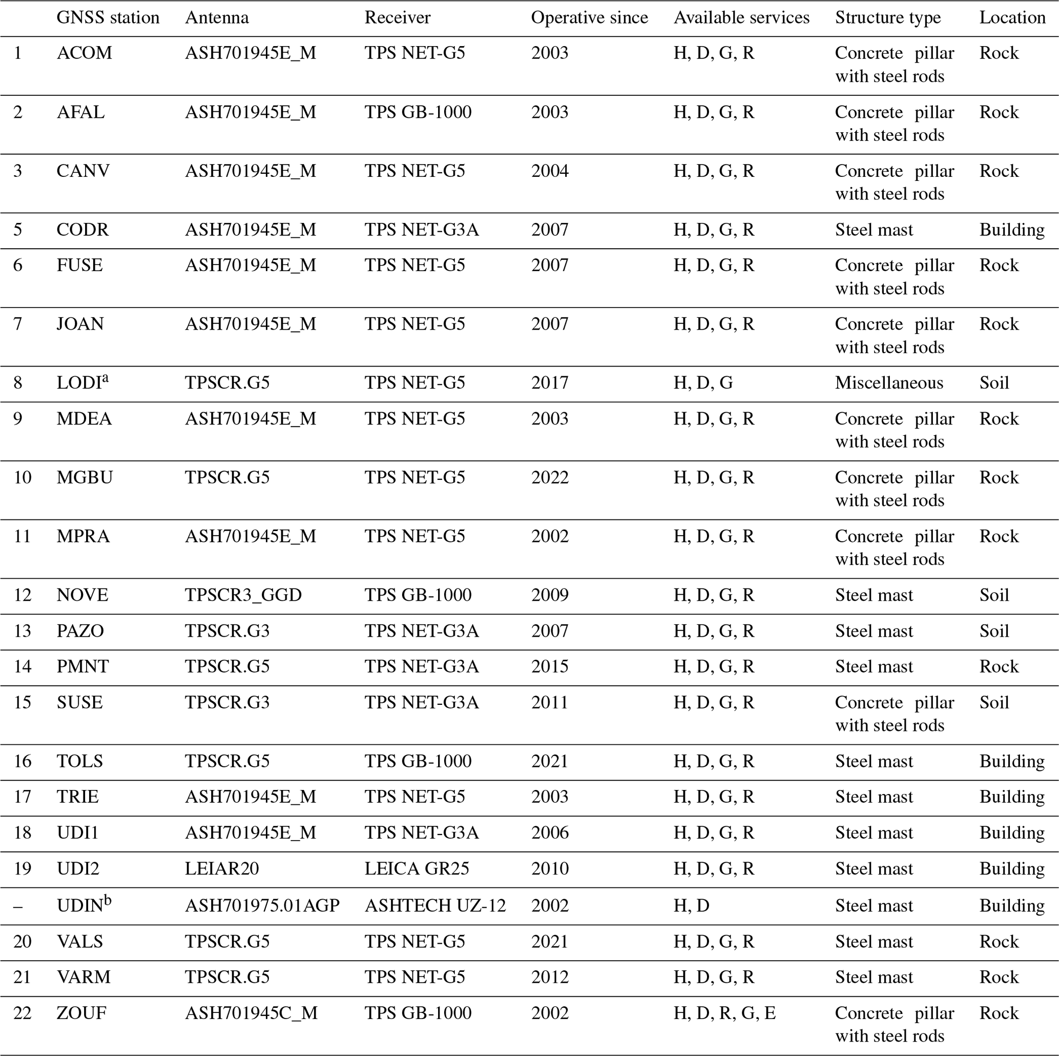
^a Station name under definition. ^b Discontinued in 2006.

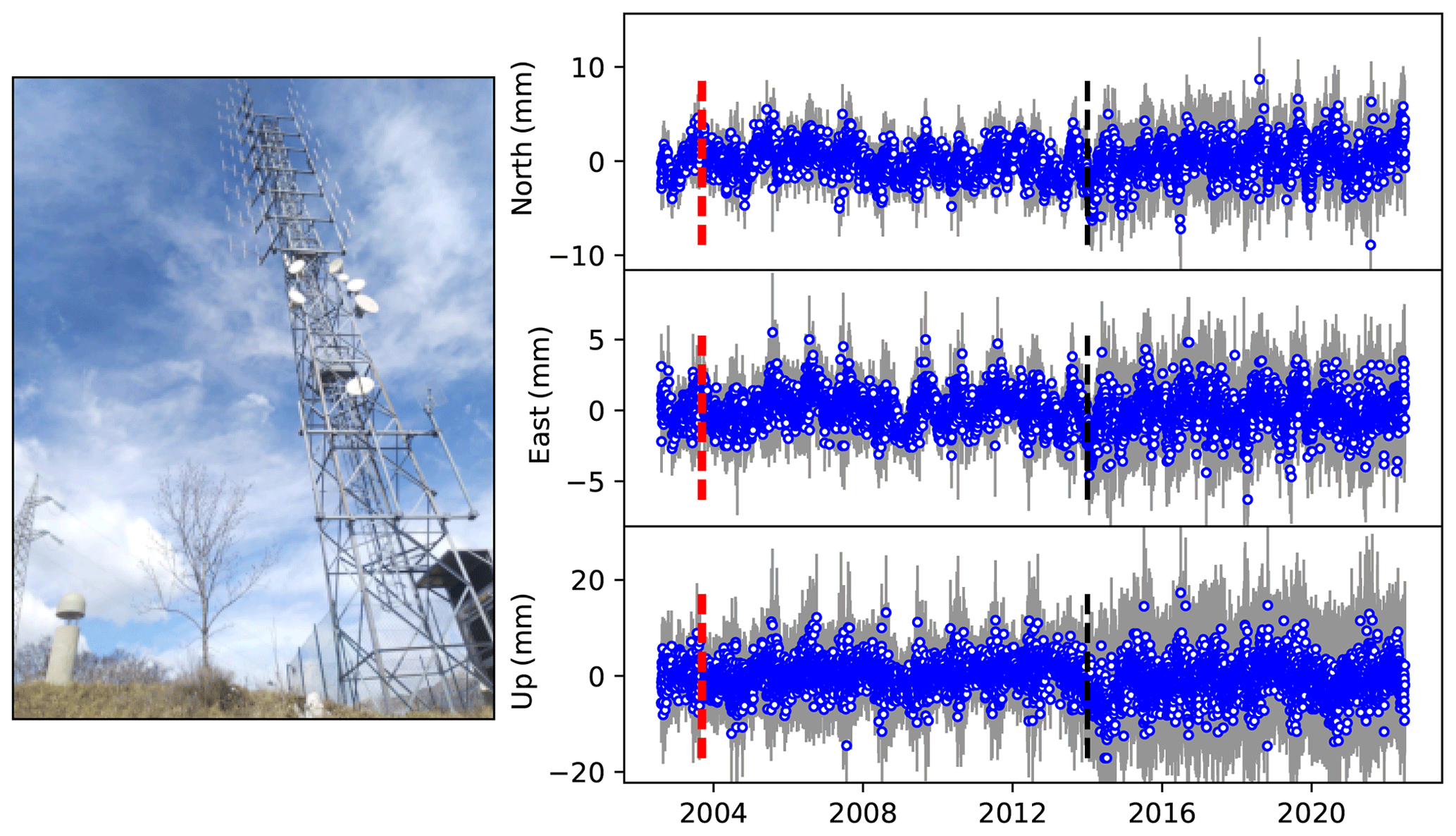
Figure A1 MPRA station photo and time series of the residuals. The red dashed line indicates a change in the antenna, while the black dashed line indicates the approximate date of the installation of the electricity pylon shown in the photo.

Appendix B: List of the GNSS networks

Table B1 List of the GNSS networks that we use to collect, archive and process the daily RINEX data.

Appendix C: Daily local data processing

We implemented on a local machine the processing procedure described in Sect. 3 of the main text with the aim of processing the data following 30 June 2022. We have made the procedure automatic for daily processing. The local machine is a Mac mini equipped with a Mac OS X (10.13) operating system. We use the crontab utility to manage the download of required input files, the update of metadata and the computation of daily solutions. From the MIT, SOPAC, CDDIS and IGS repositories, we retrieve daily updates and files about orbits, atmospheric and tropospheric parameters, satellite aircraft and ground station parameters, Earth orientation parameters, oceanic loading and tides, and ionospheric and navigation files. RINEX files from the FReDNet stations, EPOSA network and SLO_GPS stations are collected from OGS internal repositories. Observations from other networks are collected from the public data repositories of the networks, EPN data distribution services and the EPOS service. Observations are downloaded on a daily basis, with a check for possible missing observations in the 21 d before the processing date in order to fix possible data interruption or connectivity problems. Station metadata are also downloaded periodically in the form of site logs from the public data repositories of the networks or from the M3G service and are used to update the station information file and the file with the discontinuity.

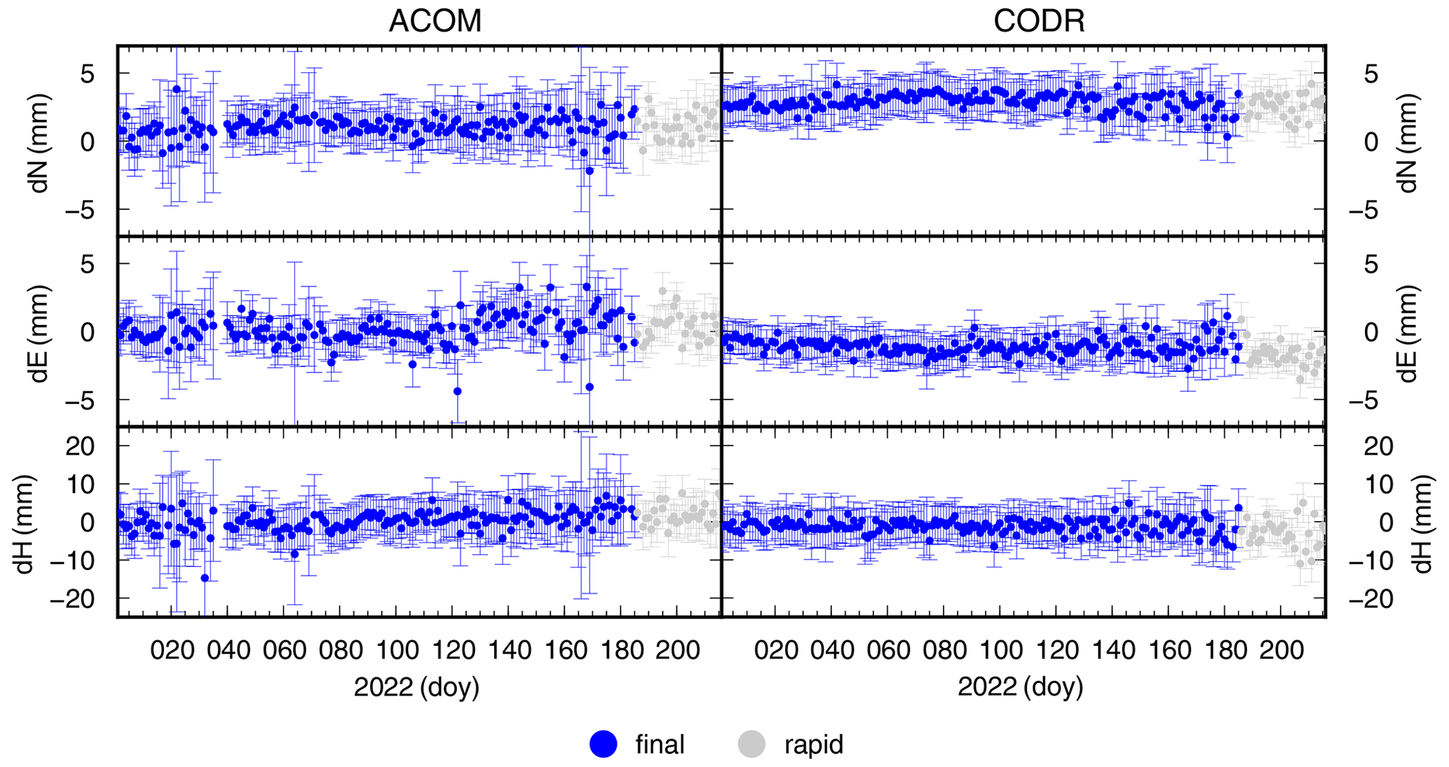
Figure C1 Coordinate time series in the ETRF14 reference framework, calculated using final orbits (blue symbols) and rapid orbits (grey symbols). Examples of ACOM and CODR stations covering the time interval 1 January 2022–4 August 2022.

The automated procedure provides two types of time series for each GNSS station: (i) coordinate time series obtained using IGS final orbit files (more precise) and (ii) coordinate time series obtained using IGS rapid orbit files, which are less precise but are available with just 3 d latency (https://cddis.nasa.gov/Data_and_Derived_Products/GNSS/orbit_products.html, last access: 12 January 2024). In particular, coordinate time series are calculated using final orbit files until 30 d before the processing date and using rapid orbit files until 3 d before the processing date. An example of the resulting time series is given in Fig. C1.

Once the daily processing is finalized, an automatic e-mail message is sent to the data analysts with the summary of the processing results.

Finally, a periodic download of the latest tar file containing incremental updates for GAMIT/GLOBK software is planned in order to keep the software updated. We also plan to update the velocity solution each year.

Appendix D: Reference sites

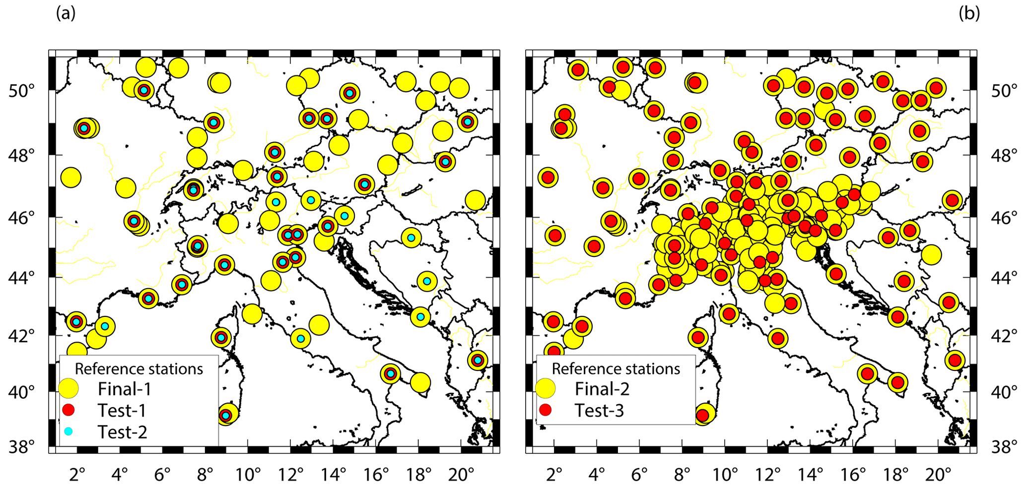
Figure D1 Reference sites used in the tests (Test-1, Test-2 and Test-3) illustrated in Sect. 5.1, plotted as red and cyan circles, compared to the reference sites used in the final processing (Final-1 and Final-2 indicate the first and second iterations, respectively, of the velocity calculation explained in Sect. 3), plotted as yellow circles.