the Creative Commons Attribution 4.0 License.
the Creative Commons Attribution 4.0 License.
 | 26 Feb 2024
Laboratory data linking the reconfiguration of and drag on individual plants to the velocity structure and wave dissipation over a meadow of salt marsh plants under waves with and without current
Heidi Nepf
Salt marshes provide valuable ecosystem services, which are influenced by their interaction with currents and waves. On the one hand, currents and waves exert hydrodynamic forces on salt marsh plants, which shapes the distribution of species within the marsh. On the other hand, the resistance produced by the plants can shape the flow structure, turbulence intensity, and wave dissipation over the canopy. Because marsh plants are flexible structures, their reconfiguration modifies the drag felt by the plants and the flow. While several previous studies have considered the flexibility of the stem, few studies have considered the leaf component, which has been shown to contribute the majority of plant resistance. This paper reports a unique dataset that includes laboratory measurements of both the force on an individual plant and the flow structure and wave energy dissipation over a meadow of plants. In the individual plant experiment, the motion of the plant and plant drag, free-surface displacement, and velocity profile were measured. The individual plant experiments considered both a live marsh plant (Spartina alterniflora) and a mimic consisting of 10 leaves attached to a central stem. For the meadow experiment, velocity profiles were measured both upstream and within the meadow, and free-surface displacement was measured along the model marsh plant meadow with high spatial and temporal resolution. These experiments used five water depths (covering both submerged and emergent conditions), three wave periods (from long wave to short waves), seven wave heights (from linear to nonlinear waves), and six current conditions (including pure current, pure wave, and combined current and wave). In summary, there are 102 individual plant tests and 58 meadow tests. The drag, free-surface displacement, and velocity are reported in the SMCW.mat and SMCW.nc files including the raw data, the phase averages, and the statistical values. A link to the plant motion videos is also provided. This dataset provides high-quality measurements that can be used to develop and validate models of plant motion, hydrodynamic drag on individual plants, vegetation-generated turbulence, the evolution of flow structure through a meadow, and the transformation and dissipation of waves over natural salt marshes. The dataset is available from Figshare with detailed instructions for reuse (https://doi.org/10.6084/m9.figshare.24117144; Zhang and Nepf, 2023a).
- Article
(2608 KB) - Full-text XML
- BibTeX
- EndNote


Salt marshes are a common feature of coastal and estuary regions, serving as important habitats and food sources for intertidal invertebrates and small fish (Boesch and Turner, 1984; Barbier et al., 2011). These marshes also play a crucial role in carbon sequestration, accumulating carbon stocks at a rate of 210 g cm−2 yr−1, the highest among all ecosystems on Earth (Pidgeon, 2009). Additionally, salt marshes provide shoreline protection by dissipating waves (Zhang et al., 2020; Garzon et al., 2019b), reducing erosion, and enhancing sedimentation (Schoutens et al., 2019; Elschot et al., 2013; Huai et al., 2021). The health and function of salt marsh ecosystems depend on the interaction between the marsh and surrounding currents and waves. Currents and waves exert hydrodynamic forces on marsh plants, influencing the distribution of species within the marsh (Schoutens et al., 2022, 2020). In addition, because marsh plants are flexible, they reconfigure under hydrodynamic forces, modifying the forces experienced by the plants (Zhang and Nepf, 2021b) and the impact of plant resistance on flow structure (Chen et al., 2013; Lowe et al., 2005; Zeller et al., 2015; Lei and Nepf, 2021), turbulence intensity (Xu and Nepf, 2020), and wave energy transformation (Hu et al., 2014; van Veelen et al., 2020; Vuik et al., 2016).
Theories that quantify the hydrodynamic force on rigid cylinders and flat plates were developed in the 1950s (Morison et al., 1950; Keulegan and Carpenter, 1958). However, real plants are flexible and reconfigure under the influence of currents and waves, reducing the hydrodynamic forces they experience (Luhar and Nepf, 2011; Gosselin et al., 2010; Mullarney and Henderson, 2010; Zhu et al., 2020). Models have been developed to predict the forces on flexible structures by considering the reconfiguration and relative motion between the fluid and the plant (Luhar and Nepf, 2011; Mullarney and Henderson, 2010; Gosselin et al., 2010; Lei and Nepf, 2019b). Laboratory measurements have shown that real plants with different morphologies follow different scaling laws (Harder et al., 2004; Schutten and Davy, 2000; Jalonen and Järvelä, 2013; Whittaker et al., 2013; Zhang and Nepf, 2020). Many salt marsh plants consist of multiple flexible leaves attached to a single, less flexible central stem, e.g., Phragmites australis, Scirpus maritimus, Spartina alterniflora, and Spartina anglica. For these plants, the rigidity and geometric properties as well as the density of the leaves and stem affect the drag and hence the wave dissipation by the plants (Zhu et al., 2023). Zhang and Nepf (2021b) demonstrated that the force acting on a full plant can be estimated by summing the forces on all the leaves and the stem, while applying a sheltering coefficient to account for the plant drag reduction due to the interaction and sheltering among the leaves and the stem. The sheltering coefficient depends on the geometric properties of the plant (mainly the distribution of leaves on the stem) and does not vary with flow conditions. Based on this, predictive models were proposed to estimate the forces acting on salt marsh plants with both leaves and stem (Zhang and Nepf, 2021b, 2022).The plant rigidity, morphology, and spatial distribution vary significantly in the field, which makes the estimation of plant drag and wave dissipation difficult in practice. Fortunately, average values of plant properties have been shown to produce a reasonable estimation for field measurements of wave dissipation (Zhang and Nepf, 2021b; Zhang et al., 2022, 2021; Zhu et al., 2023).
Within a canopy, the presence of plants can significantly alter the flow structure (Chen et al., 2013; Lowe et al., 2005; Zeller et al., 2015; Lei and Nepf, 2021) and turbulence intensity (Xu and Nepf, 2020) and reduce wave energy (Garzon et al., 2019a; Zhang et al., 2020; Maza et al., 2015). The fully developed flow structure within a canopy has been extensively studied under both current (Chen et al., 2013; Lei and Nepf, 2021) and wave conditions (Lowe et al., 2005) for both emergent and submerged canopies. Specifically, the mean flow is determined by the distribution of the plant frontal area for emergent canopies and by the canopy drag and the ratio of water depth to plant height for submerged canopies (Nepf, 2012). The wave orbital velocity experiences less modification by a canopy due to the greater inertial force under waves compared to currents (Lowe et al., 2005), which allows flow motion to penetrate deeper into the lower canopy region. The presence of plants affects turbulence intensity directly through form drag and wakes generated by plant elements and indirectly by adjusting the flow structure to create a greater shear and thus shear production (Nepf, 2012). The resistance of plants can reduce wave height by 30 % to 90 % over the first 30 m of a salt marsh (Ysebaert et al., 2011; Knutson et al., 1982; Zhang et al., 2020; Garzon et al., 2019a), depending on the plant properties (density, geometry, and mechanical characteristics) and flow conditions (water depth, wave period, wave amplitude, presence of currents). Recent studies proposed simple predictions for wave decay over salt marshes under pure waves (Zhang et al., 2021, 2022), which has been extended to combined current and wave conditions using the in-canopy total velocity (Zhang and Nepf, 2021a). Using the data provided in the present paper, a theoretical model for the time-varying total velocity has been developed for salt marshes under combined currents and waves (Zhang et al., 2024).
This paper presents both force measurements on individual salt marsh plants (Zhang and Nepf, 2021b, 2022) and measurements of flow structure and wave decay along a meadow of salt marsh plants (Zhang et al., 2021, 2022; Zhang and Nepf, 2021a). The experiments utilized model plants that consisted of multiple flexible leaves attached to a central stem, which were designed to be geometrically and dynamically similar to Spartina alterniflora. The Spartina spp. family is distributed widely along the coasts of the eastern United States, Europe, South America, and China (see the global distribution in Fig. 1B in Borges et al., 2021). The test conditions varied from submerged to emergent, from long to short waves, and from linear to nonlinear waves with and without following currents. In total, 102 individual plant tests and 58 meadow tests were conducted.
The experiments were conducted in the Nepf Fluid Mechanics lab at MIT in a 24 m long, 38 cm wide, 60 cm tall water channel (Fig. 1). The individual plant experiments (denoted by IE, Fig. 1a) provided synchronized measurements of plant drag and free-surface displacement, as well as three-dimensional velocity profiles provided as raw data, phase-averaged data, and statistical data. Additionally, a link to videos capturing the motion of the plants is provided. The meadow experiments (denoted by ME, Fig. 1b) provide time-varying measurements of free-surface displacement along the meadow at 10 and 15 cm intervals, as well as velocity profiles upstream of and within the meadow with 1 to 2 cm vertical resolution. This dataset can facilitate the development and validation of dynamic marsh plant models, enhance predictions of marsh plant drag, and deepen our understanding of vegetation-induced turbulence, the evolution of flow structure within a canopy, and the transformation and dissipation of waves in natural salt marshes.
Monochromatic waves were used in all cases, with waves generated with a piston-type wave maker. A beach with 1:5 slope covered with a layer of 10 cm thick coconut fiber was located at the downstream end of the channel, which limited the wave reflection to 7 %±3 % for the tested conditions. Following currents (propagating in the same direction as the waves) were generated by a variable-speed pump. Two bricks elevated the beach by 9 cm above the bed to allow the current to pass.
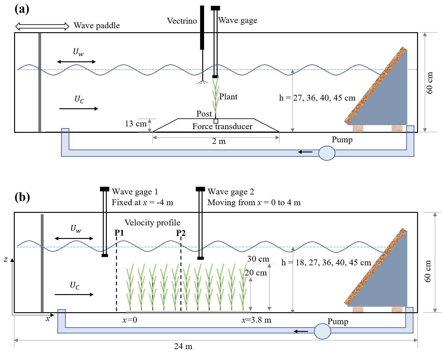
Figure 1Schematic of (a) the individual plant experiment (IE) and (b) the meadow experiment (ME), not to scale. The wave paddle and current inlet are at the left, and the wave-absorbing beach is at the right. In panel (a), the model plant was attached to a submersible force sensor housed in a 13 cm high acrylic ramp. A wave gauge recorded the free-surface displacement at the same longitudinal position as the plant, but 9 cm to the side. A Nortek Vectrino+ measured velocity 10 cm upstream of the plant position, but with the plant removed. In panel (b), the model meadow was 3.8 m long and located at mid-length along the flume. Two wave gauges measured the wave height at a stationary reference position (wave gauge 1) and at multiple positions along the meadow (wave gauge 2). Velocity in front (P1) and inside the meadow (P2) was measured by Vectrino+.
2.1 Individual plant experiment setup
The individual plant experiments (IE) tested a live Spartina alterniflora, a single flat plastic leaf, a single cylindrical stem, and a full model marsh plant consisting of 10 leaves attached to a central stem. These tests are labeled as live, leaf, stem, and model, respectively. Figure 2 shows the live and model plants with the corresponding plant properties (see also Fig. 2 and Table 1 in Zhang and Nepf, 2021). The live plant consisted of five leaves, and the dimensions shown in Fig. 2a are the mean ± SD of these leaves. The plant was attached to a stainless-steel post with 2 mm diameter. The length of the post above the ramp was lp=3, 4.5, 2, and 2 cm for the live, leaf, stem, and model plant, respectively. The lower part of the post was attached to a submersible force sensor (Futek LSB210 100g), which was mounted beneath an acrylic ramp (1 m top length, 2 m bottom length, 13 cm height, and spanning the flume width, see Fig. 1a) to avoid interaction between fluid motion and the sensor. IE measured the hydrodynamic force exerted on the plant, the motion of the plant, and the associated hydrodynamic conditions (velocity profile and wave height). The wave gauge was mounted at the same longitudinal position as the plant, but 9 cm to the lateral side. Note that for each plant and each water depth, the zero position of the wave gauge and force sensor was determined for still water, i.e., before the wave generator and current pump were turned on.
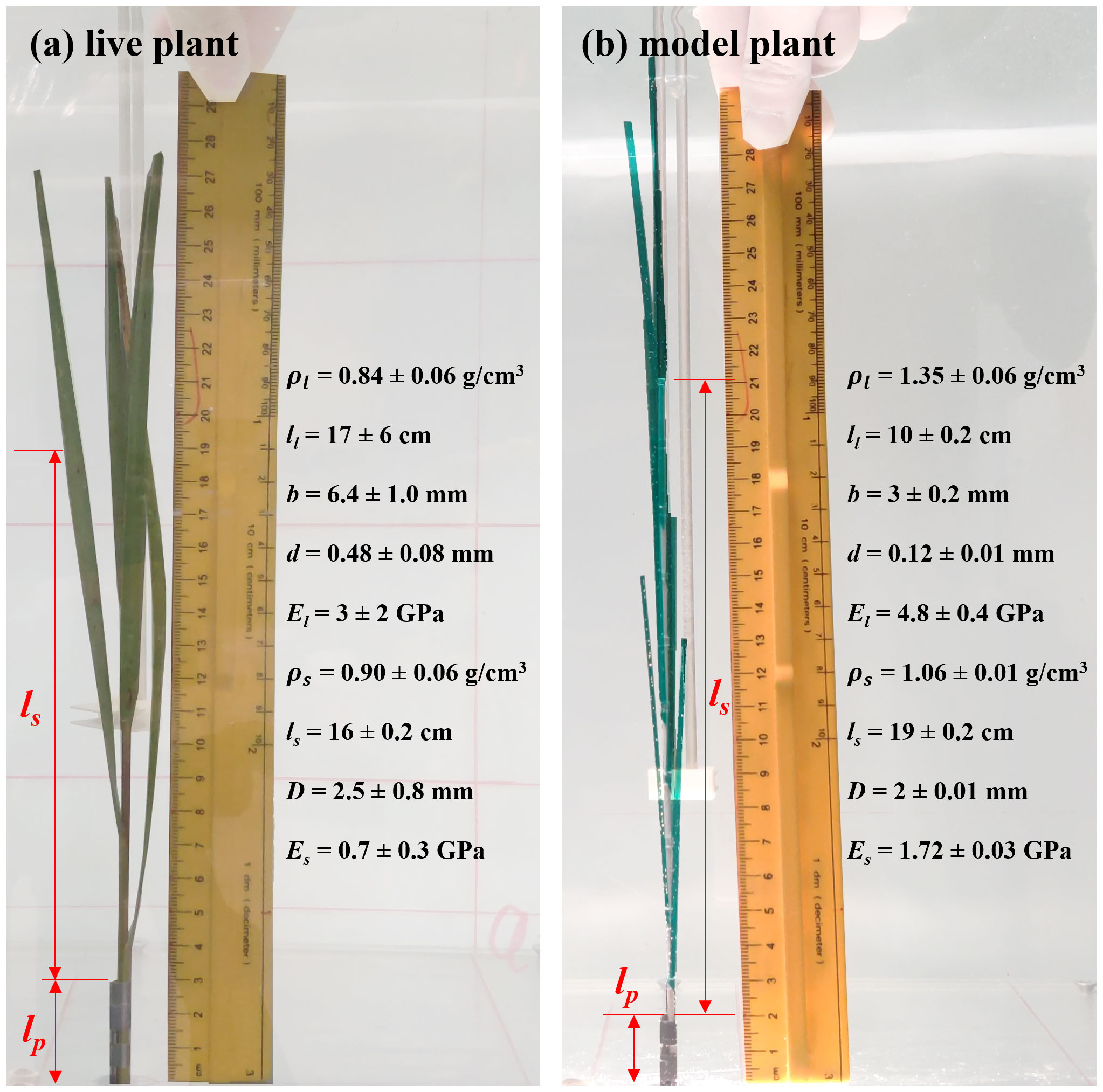
Figure 2Photos showing (a) the live plant and (b) model plant in the individual plant experiment (IE), including a list of plant properties. ρ is the plant material density, and the subscripts p, l, and s denote parameters for the post, leaves, and stem, respectively. E is the elastic modulus, l is the element length, and b and d are the width and thickness of the leaf. D is the stem diameter.
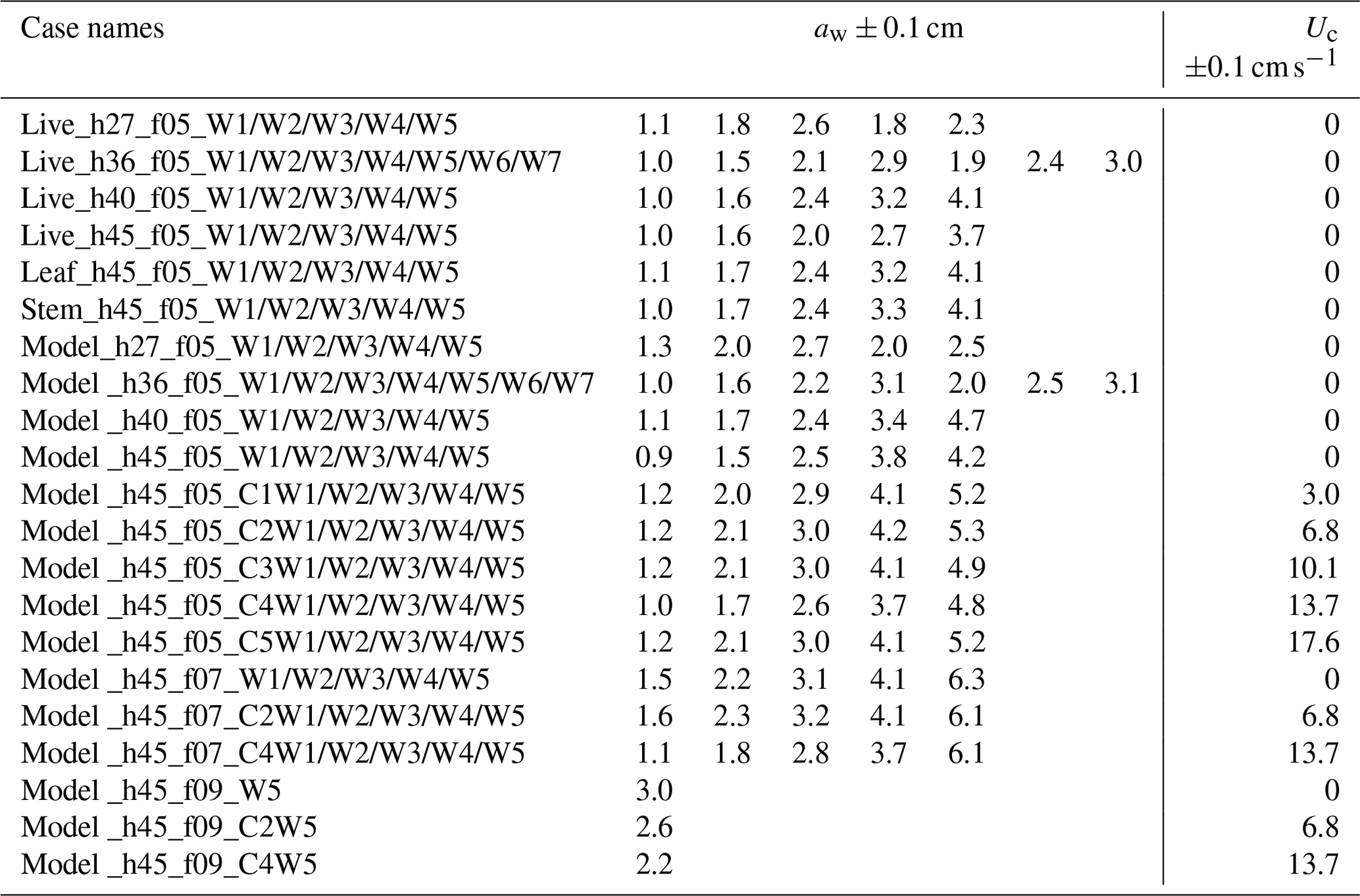
IE tested four water depths at h=27, 36, 40, and 45 cm for the live and full model plant. The leaf- and stem-only tests were done under h=45 cm. Note that the leaf data reported here correspond to an initial vertical leaf posture, and the leaf width was oriented perpendicular to the wave propagation direction (i.e., leaf posture 1 in Fig. 4a in Zhang and Nepf, 2021b). Three wave periods, Tw=2.01, 1.44, and 1.12 s, and six wave amplitudes were tested. All the tested conditions are summarized in Table 1, with the case names formed from the type of plant (live, leaf, stem, model), the water depth (h27, h36, h40, h45), the wave frequency (f05, f07, and f09), and the wave height setting (W1, W2, W3, W4, W5, W6, W7, aw ranging from 0.9 to 4.9 cm). The current conditions were labeled by pump frequency (10 to 50 Hz) as C1, C2, C3, C4, and C5. For example, Leaf_h45_f05_C1W1 corresponds to the test for an individual model leaf with water depth h=45 cm, wave period Tw=2.01 s (wave frequency is 0.5 Hz), current pump frequency set to 10 Hz, and the smallest wave height (wave amplitude aw≈1 cm). The tests include the pure wave experiment reported in Zhang and Nepf (2021) and the combined current and wave experiments reported in Zhang and Nepf (2022). In addition, there are 23 unreported cases labeled with bold font in Table 1 (6 model plant cases and 17 live plant tests). The new live plant tests included emergent conditions, which can be used to explore the plant drag dependence on the degree of submergence. The new model plant cases included a stronger wave condition (aw=4.7 cm) and five conditions within the published range of wave height. These new cases expanded the range of published flow conditions. Across the IE tests, the wave orbital velocity spanned Uw=4 to 24 cm s−1 and the channel-average current spanned Uc=3 to 18 cm s−1. The current to wave velocity ratio spanned to 4.7, covering a range of conditions present in the field (Garzon et al., 2019b).
Table 1IE case names with the measured wave amplitudes and the setting current velocity.
The force sensor and wave gauge were controlled by a Labview program, which enabled high-quality synchronous measurement. Both the drag force and wave height were measured at a sampling rate of 2000 Hz and for a duration of 3 min. During the force and wave gauge measurements, a smart cell phone (MIX 2S) camera recorded a 10 s UHD 4k video at 30 fps, which covered 5 to 10 wave periods, depending on the wave period. The camera was fixed to a tripod such that the videos for each plant have the same window. The videos for all tests are available at https://doi.org/10.6084/m9.figshare.24117324 (Zhang and Nepf, 2023b). After the force measurements, the plant and force sensor were removed, and a Nortek Vectrino+ was used to measure the velocity profile 10 cm upstream of the position where the plant had been to avoid the hole through which the plant was attached. The vertical resolution of the velocity profile was 1 cm. At each measurement point, the Vectrino recorded a 3 min record at 200 Hz.
2.2 Meadow experiment setup
In the meadow experiment (ME), the same model plants used in IE (Fig. 2b) were arranged in a staggered array with a meadow density of 280 plants m−2 (Fig. 3). Once inserted, the erect plants were 30 cm tall. The plants were distributed across the channel width and over a streamwise distance of 3.8 m.
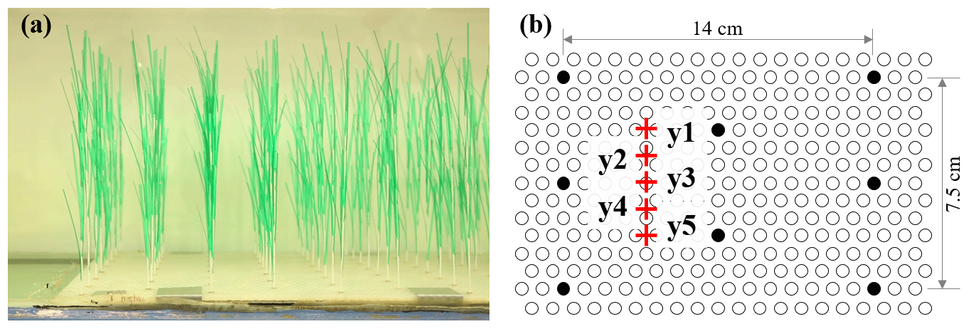
Figure 3(a) Photo of the model plants and (b) section of the baseboard with staggered holes (circles) and the plant positions within the hole array (filled circles).
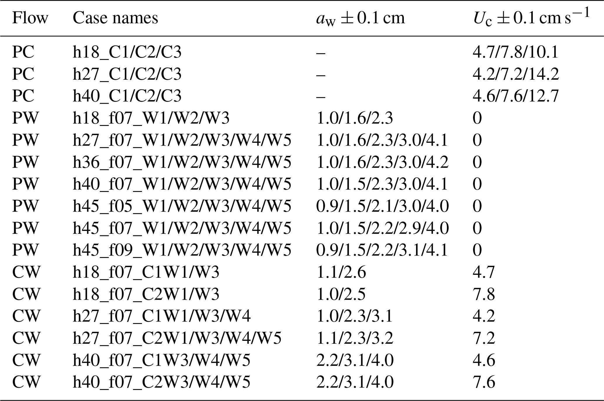
ME tested five water depths of h=18, 27, 36, 40, and 45 cm, three wave periods of Tw=2, 1.4, and 1.1 s, five wave amplitude levels, and three current magnitudes. All the ME cases are summarized in Table 2 with the case names formed based on the flow conditions in the same way as IE cases. The flow types include pure current, pure wave, and combined current and wave, which are labeled PC, PW, and CW, respectively. In each case, two wave gauges were synchronized to measure the free-surface displacement at a reference position (wave gauge 1 at m) and at positions along a transect through the canopy (wave gauge 2). During each experimental run (about 90 min), the wave amplitude at wave gauge 1 varied by less than 3 %, confirming stationary wave conditions. Wave gauge 2 collected data between and 4 m at 10 and 15 cm intervals. The leading edge of the meadow was located at x=0 such that x<0 was over bare bed. At each position, the free-surface displacement, η(t), was recorded at 2000 Hz for 1 min. Additional measurements of wave amplitude were made without plants to assess the wave decay associated with the channel wall and baseboards alone.
Table 2ME case names with the measured wave amplitudes and the setting current velocity.
Two Nortek Vectrino+ devices were used to measure the vertical profiles of velocity with 1 to 2 cm vertical resolution at P1 (upstream of the meadow) and P2 (within the meadow) (Fig. 1b). At each measurement point, the Vectrino+ recorded a 1 min record with a sampling frequency of 200 Hz. Upstream of the meadow, velocity was measured at the channel centerline. Inside the meadow, velocity measurements were made at one lateral location (y2 or y4 in Fig. 3b, as in Zhang et al., 2022, 2021) or five lateral locations near the flume centerline (red pluses in Fig. 3b, as in Zhang and Nepf, 2021a).
2.3 Data analysis
The free-surface displacement, force, and velocity data were processed in a similar fashion. First, the analysis of wave data will be described in detail. The wave gauge has an accuracy of 0.2 (0.7) mm on average (maximum) based on the standard deviation of the raw data under still-water conditions. For each record, the mean surface position was removed from the time series to obtain the free-surface displacement data η. The surface displacement time series was separated into phase bins (Lei and Nepf, 2019b; Zhang and Nepf, 2021a). Specifically, for sampling duration T, a wave measurement record contains wave periods, with “floor” denoting a downward rounding function. Each wave period contains γ=Twfs samples and thus γ phase bins. fs is the sampling frequency. The phase-averaged free-surface displacement in the nth phase bin (n=1 to floor(γ)), corresponding to phase , was defined as
denotes the phase-averaged value. Within each phase bin, the standard deviation of was 0.7 (3.6) mm on average (maximum) based on the IE tests. Increasing current intensity led to higher uncertainty in . The wave amplitude aw was calculated from the root-mean-square surface displacement,
For ME, the spatial evolution of wave amplitude can be used to estimate the wave damping by vegetation. However, note that the wave amplitude reflected the sum of the incoming wave and the beach-reflected wave, the superposition of which resulted in an amplitude modulation at an interval of (with wavelength λ, e.g., Fig. 4). Accounting for the wave modulation, the wave decay coefficient KDf was estimated by fitting the measured amplitudes (Lei and Nepf, 2019b),
in which is the wavenumber, and ϵ, C1, and C2 are fitting parameters. Examples are shown in Fig. 4. Wave decay attributed to the plants (KD, m−2) was obtained by subtracting the decay coefficient obtained in the flume without plants.
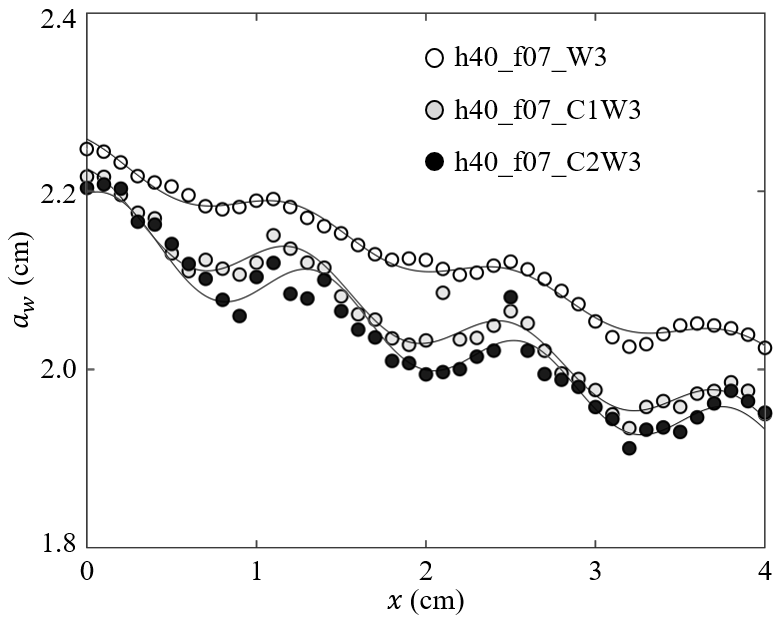
Figure 4Measured wave amplitude (symbols) and the fitted Eq. (3) (curves) for h40_f07_W3, h40_f07_C1W3, and h40_f07_C2W3 with a similar wave amplitude but increasing current (adapted from Fig. 4 in Zhang and Nepf, 2021a).
For the individual plant experiments, a time lag of d ms (SD) was determined between the force sensor and wave gauge due to the difference between the instruments' reaction times. This time lag was accounted for by removing the free-surface displacement records (about 148 data points) before the first force sensor record. The FFT (fast Fourier transform) function in MATLAB was used to filter out high-frequency noise (frequency components greater than 2 Hz), which was negligible based on the frequency spectrum and was subtracted from the raw data. The plant force time series, F, was obtained by removing the offset measured with still-water conditions. The phase-averaged plant drag, , was obtained in similar way as Eq. (1). The maximum, minimum, and mean values of are reported as Fmax, Fmin, and Fm, respectively. For pure current conditions, Fm was defined by the average over the 3 min record.
Based on the standard deviation among 10 still-water measurements, considering different water depths and different plants installed on the force sensor, the accuracy of the force measurements was determined to be 0.001 N (0.002 N) average (maximum). The force exerted on the post alone (without plant) was less than 3 % of the force on the model plant (Zhang and Nepf, 2021b, 2022). Consequently, in this dataset, the force due to the post was neglected and not subtracted from the measurements. However, note that the force on the post can contribute up to 30 % of the total force measured for an individual leaf. Hence, when using the leaf force data, it may be necessary to exclude the force due to the post.
For all velocity data, two despiking methods were applied to identify abnormal data points, which were replaced by a NAN (not a number) value. First, data points were identified if the associated acceleration exceeded the gravitational acceleration. Second, a threshold, ±3σ, with σ the standard deviation, was applied to identify abnormal data within each phase bin for conditions with waves and in the whole time series for the pure current cases (Zhang and Nepf, 2022). The despiked velocity data are denoted u, v, and w for the longitudinal, lateral, and vertical directions, respectively. For the horizontal velocity component, the velocity data were separated into a phase-averaged value and a turbulent velocity fluctuation u′,
was calculated in the same manner as Eq. (1) and then further separated into a time-mean velocity , and the wave orbital velocity was defined as . The magnitude of wave orbital velocity was defined as
The root mean square of the fluctuating velocity component within each phase bin was used to estimate the turbulent kinetic energy in that phase bin, . The time-average turbulent kinetic energy, TKE, was defined as the average of tke(ϕ) over all phases. The depth- and phase-averaged horizontal velocity was defined as . The depth-average velocity statistics reported for each velocity profile include the maximum Umax, minimum Umin, and mean Um value of . The depth-average wave orbital velocity was defined as . For pure current cases, Um=Uc was defined by the depth- and time-averaged velocity over all measurements. The phase-averaged and depth-averaged values for the lateral (v) and vertical (w) velocity components were calculated in the same way as the horizontal component.
3.1 Data for the individual plant experiments (IEs)
In experiments with individual plants, the plant force and free-surface displacement at the same streamwise (x) location as the plant were measured simultaneously. The motion of the plant was captured in videos during the force measurement. The flow velocity was measured separately but assumed to be in phase with the free-surface displacement. These data contained all relevant parameters necessary for understanding the hydrodynamic performance of an individual marsh plant. For example, Fig. 5 shows the maximum plant motion, phase-averaged plant drag and free-surface displacement, and the phase- and depth-averaged velocity for the model plant under the same wave with and without a following current. These data demonstrate a strong dependence of plant force on the instantaneous flow velocity, which can be utilized to validate predictions of plant drag, as in Zhang and Nepf (2022, 2021b). It is worth noting that the phase-averaged data allow for detailed validation of phase-resolving models. Only a few studies, e.g., Jacobsen et al. (2019) and Luhar and Nepf (2016), have reported time-varying velocity and force on flexible plants. However, for modeling and validating plant motion and time-varying plant force, high-resolution time-varying horizontal and vertical velocity is required. For example, Zhu et al. (2020) demonstrated that the vertical velocity results in asymmetric plant motion, even when subjected to symmetric waves. For high-resolution model validation, the present dataset includes both the time-varying horizontal and vertical velocity, as well as the synchronized force and free-surface displacement for both live and model plants.
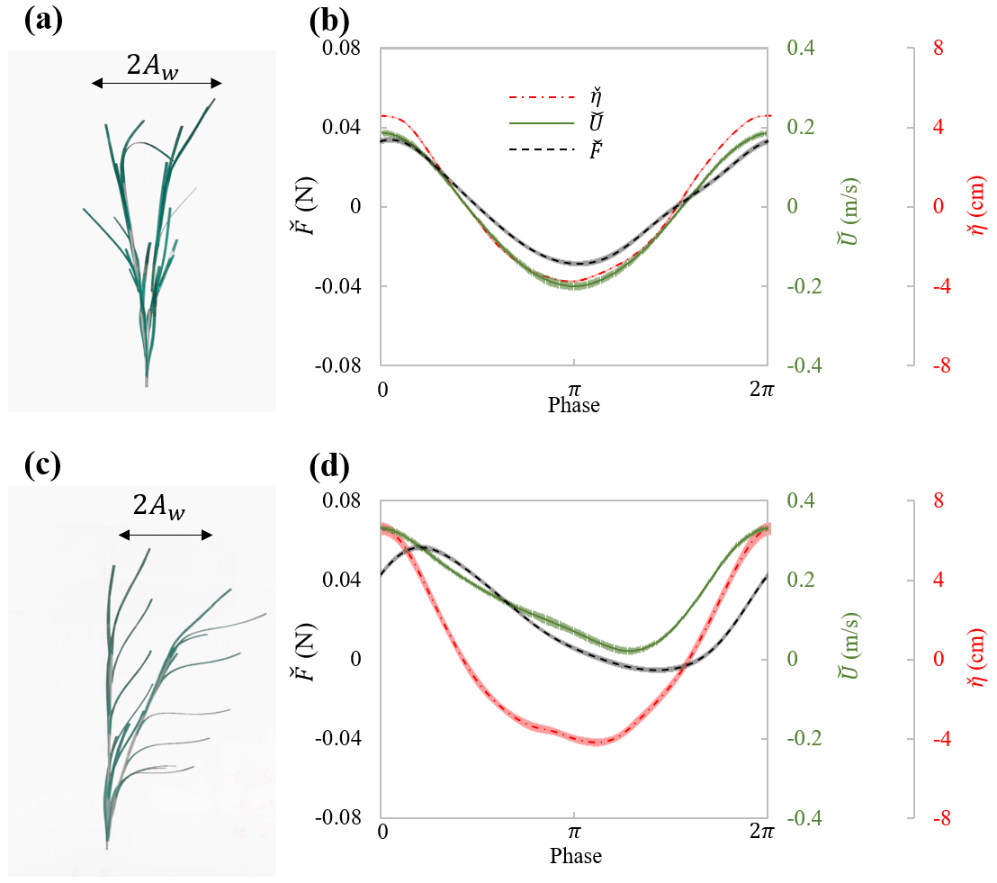
Figure 5Plant motion and phase-averaged measurements of force (black curve), surface displacement (red curve), and velocity (green curve) for (a, b) model_h45_f05_W5 ( and Uw=19.1 cm s−1) and (c, d) model_h45_f05_C5W5 ( and Uw=14.3 cm s−1). Panels (a) and (c) show the digital image of the model plant at the maximum downstream and upstream posture within the wave cycle. The thin shading in each curve in panels (b) and (d) indicates the uncertainty in each phase (modified based on Fig. 5 in Zhang and Nepf, 2022.)
The force measurements suggested that the force on the full plant was smaller than the sum of forces on all the leaves and stem acting alone, suggesting that sheltering and interaction among the leaves and stem decreased the force exerted on the full plant compared to the leaves and stem in isolation (Fig. 6a). The decrease in plant drag can be represented by a constant sheltering coefficient Cs for a given plant morphology. Specifically, for a plant with Nl leaves attached to a central stem, the force on the full plant is F (plant) (one leaf) (stem), with Cs=0.6 for the model plant reported here (Zhang and Nepf, 2021b). The leaves were estimated to contribute 72 %±1 % of the plant-scale drag (Zhang and Nepf, 2021b). With this finding, the hydrodynamic force on a plant with complex leaf and stem morphology can be easily estimated using the force prediction for an individual simple structure (a flat leaf or a cylindrical stem, e.g., the models described in Zhu et al., 2020; Mullarney and Henderson, 2010; Luhar and Nepf, 2011, 2016).
The maximum force on the plant is plotted against the maximum depth- and phase-averaged velocity in Fig. 6. Note that for h=40 and 45 cm, both the live and model plants were submerged at the wave crest (see videos at https://doi.org/10.6084/m9.figshare.24117324, Zhang and Nepf, 2023b). The maximum force for these two water depths followed the same trend with velocity (Fig. 6b and c). For smaller water depth, only part of the plant was submerged such that the plant felt a smaller force under similar horizontal velocity (Fig. 6b and c). The relationship between Fmax and Umax was similar for different current velocities, but curves were shifted to the right as the current increased (darker symbols in Fig. 6d); i.e., as current magnitude increased, a greater Umax was needed to reach the same Fmax (Fig. 6d).
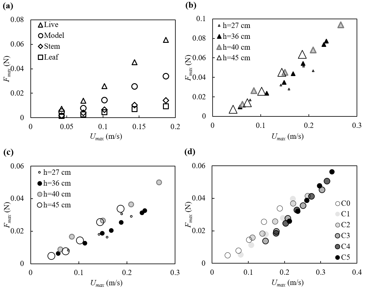
Figure 6Maximum force on the plant plotted against the maximum horizontal velocity for (a) all plants at h=45 cm, (b) the live plant and (c) the model plant under pure waves, and (d) the model plant at h=45 cm under combined current and waves with increasing current intensity labeled C0 to C5. All the cases shown are associated with wave frequency f=0.5 Hz. The uncertainty in the force measurements, not shown in the figures, ranged from 0.001 to 0.002 N based on the standard deviations of force in each wave phase.
3.2 Canopy velocity structure and turbulence
The canopy velocity structure and turbulence were altered by the plant drag, which in turn affected the dissipation of wave energy. Figure 7 shows a few examples of the turbulence and velocity structure of the ME test. First, for pure current, the presence of the canopy significantly modified both the flow structure and turbulent intensity (Fig. 7a). The time-mean velocity um at P1 (2 m upstream of the meadow) exhibited a boundary-layer velocity profile (circles in Fig. 7a2), and the TKE was essentially uniform, with a slight increase near the bed (circles in Fig. 7a1). The canopy resistance reduced um within the canopy height by a factor of 0.29 and redirected the time-mean flow above the canopy, forming a shear layer extending from the top of the stems toward the free surface (Fig. 7a2). Within the canopy, the magnitude of the horizontal velocity was negatively correlated with the distribution of plant frontal area (Nepf, 2012). Specifically, a greater time-mean velocity was observed near the bed (Fig. 7a2) where the plant frontal area was smaller (Fig. 2b). Considering that the velocity is zero at the bed, the velocity profile um exhibited an “S” shape at P2 (2.46 m inside the meadow). The time-mean velocity um at five lateral locations within the canopy (y1 to y5, red pluses in Fig. 3b) was the same within uncertainty, but the TKE was maximum directly upstream of a plant (P2_y1 and P2_y5) and minimum directly downstream of a plant (P2_y3). The maximum TKE was observed near the top of the canopy due to shear production associated with the strong vertical gradient in velocity (Fig. 7a2).
For pure waves, the turbulence intensity was maximum near the free surface and decreased with distance from the surface at P1 (circles in Fig. 7b1). Note that the time-mean velocity can be slightly negative in a closed flume, reflecting the return current that develops to balance the mass transport associated with the Stokes drift (Monismith, 2020), and its magnitude increases with distance from the bottom (Fig. 7b2). The presence of the canopy reduced the wave orbital velocity uw slightly due to the wave energy dissipation by the plants (Fig. 7b3) and adjusted the time-mean velocity to a more uniform profile (Fig. 7b2). Compared to TKE measured at P1, the turbulent intensity at P2 was larger within the canopy but similar near the top of the canopy (Fig. 7b1). Specifically, above the canopy height, TKE was primarily generated by the mean shear production, and the similar TKE at P1 and P2 can be explained by the comparable time-mean velocity profiles, i.e., comparable shear. Within the canopy, TKE was mainly generated by the plant form drag such that TKE was obviously larger compared to P1.
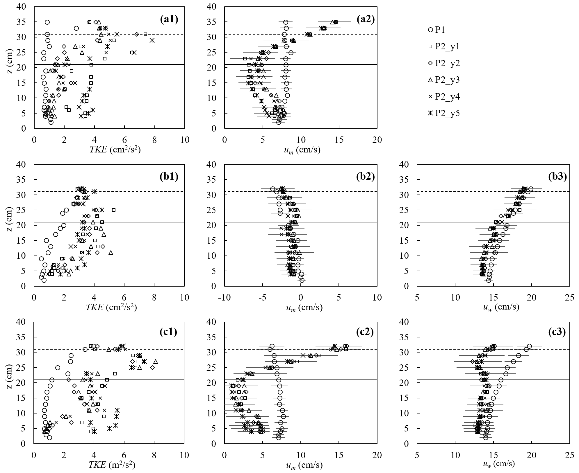
Figure 7The turbulent kinetic energy (left), horizontal time-mean velocity (middle), and wave orbital velocity (right column) for (a) pure current (h40_C2, Um=7.7 cm s−1), (b) pure waves (h40_f07_W5, , Uw=16.7 cm s−1), and (c) combined current and waves (h40_f07_C2W5, Um=7.0, Uw=15.6 cm s−1). For the cases shown, water depth h=40 cm. The measurements were made at P1 (2 m in front of the meadow at the flume center) and P2 (2.46 m in the meadow) at five lateral positions y1 to y5 shown as red plus signs in Fig. 3b. The horizontal bars indicate the average standard deviation within each phase bin. The solid and dashed horizontal lines indicate the stem height and erect canopy height, respectively.
Finally, consider the conditions with combined current and waves (Fig. 7c). Upstream of the canopy (position P1, open circles in Fig. 7), the time-mean velocity um (Fig. 7c2) and wave orbital velocity uw (Fig. 7c3) exhibited the same vertical profile shape as that observed for the pure current (Fig. 7a2) and pure wave conditions (Fig. 7b3), respectively, and TKE (Fig. 7c1) was similar in magnitude to the pure wave condition (Fig. 7b1). This might be explained by time-mean velocity gradients (Fig. 7c2 and b2), which feed shear production of turbulence and are similar in pure wave and combined wave–current conditions. Within the meadow (P2), adding a current resulted in greater decrease in uw and a more uniform profile (Fig. 7c3) compared to that under pure waves (Fig. 7b3). Smaller in-canopy wave orbital velocity was explained by greater plant drag (positively related to um+uw as in Fig. 6) and hence greater wave energy dissipation under combined conditions than the same pure wave (Zhang and Nepf, 2021a). Similarly, stronger plant resistance under combined current and waves resulted in a greater reduction in time-mean velocity within the canopy, relative to upstream compared to pure current conditions (Fig. 7c2). Specifically, for the combined wave–current conditions, um within the canopy (roughly z<30 cm) at P2 was reduced by a factor of 0.42, compared to um at P1, whereas for the pure current condition the reduction was only a factor of 0.29. Finally, in combined wave–current conditions, the TKE within the meadow (P2) was greater than TKE for either the pure current or pure wave conditions (comparing the left column in Fig. 7). This was consistent with the greater reduction in in-canopy current and greater dissipation of wave energy because energy lost from time-mean and wave energy is converted into turbulent kinetic energy. In addition, in the combined wave–current conditions two regions of high TKE were observed: one near the top of the canopy, associated with shear-generated turbulence and consistent with the pure current condition, and a second within the lower canopy, associated with plant-element-generated turbulence (Fig. 7c1).
In addition to the time-mean velocity, wave orbital velocity, and turbulent kinetic energy, the time series for each velocity component (u, v, w) as both raw data and phase-averaged velocity for all ME are contained in the dataset. This dataset can be used to describe the physical mechanisms associated with current–wave–vegetation interaction.
3.3 Wave decay over salt marsh meadow
ME measured the free-surface displacement at 2000 Hz, with a spatial interval of 10 or 15 cm along the meadow length. These data can be used to examine the wave amplitude dissipation (as in Zhang et al., 2021, 2022; Zhang and Nepf, 2021a) and wave shape transformation over a salt marsh meadow. The wave decay coefficient, KD, increased with decreasing water depth and decreasing wave amplitude (Fig. 8). For a constant water depth (circles in Fig. 8), as wave period increased from Tw=1.12 s to 1.44, KD increased, but then remained the same within uncertainty between Tw=1.44 and 2.01 s. The dependence of KD on water depth, wave amplitude, and wave period can be explained by how these parameters affect the fluid velocity and drag on the plant. First, for the same aw and Tw, Uw increases with decreasing h, generating greater plant drag and thus greater wave energy dissipation as water depth decreases. Second, for a constant depth (h=45 cm) and wave amplitude, an increase in wave period (here, Tw=1.11, 1.44, and 2.01 s) produces a decrease in dimensionless wave number kh =1.55, 1.08, and 0.77, respectively. This decrease in kh is associated with a wave velocity profile that is increasingly more uniform, producing larger depth-averaged velocity magnitude (see Fig. B.1 in Zhang et al., 2022). Finally, with constant depth and wave period, an increase in wave amplitude results in greater plant motion within the wave cycle, which leads to a greater reduction in the plant drag (due to greater plant reconfiguration) and wave dissipation. Detailed mechanisms and a scaling analysis are provided in Zhang et al. (2022).
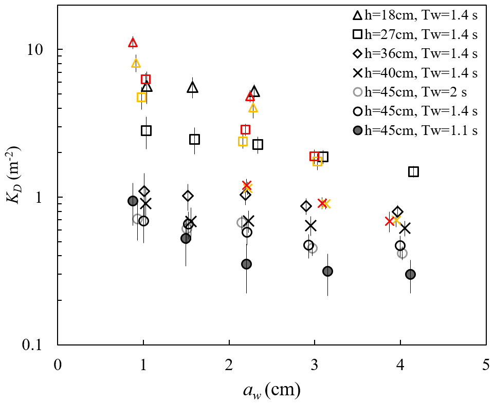
Figure 8Wave decay coefficients KD for all cases reported (Zhang and Nepf, 2021a; Zhang et al., 2021, 2022). The yellow and red symbols indicate waves with small (Uc=4.7 cm s−1) and larger (Uc=7.8 cm s−1) following currents, respectively. The vertical bars indicate uncertainty in KD (adapted from Fig. 4a in Zhang et al., 2021).
Adding a following current tended to increase wave dissipation. For the same water depth and wave period, KD increased with increasing current magnitude (red and yellow symbols in Fig. 8) compared to pure wave conditions (black symbols in Fig. 8) with similar wave amplitude. The effect of a following current increasing wave dissipation is shown more clearly in Fig. 9, which shows the ratio of wave decay coefficient in combined current and wave conditions (KD,cw) normalized by the value in pure waves (KD,pw). Generally, as current increased, increased above 1. There were a few exceptions for , for which adding a weak current slightly reduced the wave decay coefficient, i.e., . This opposite effect of current on wave decay has been reported in a few previous studies (Hu et al., 2014; Li and Yan, 2007; Yin et al., 2020; Paul et al., 2012; Losada et al., 2016; Zhao et al., 2020). Paul et al. (2012) attributed the reduction in wave dissipation with current mainly to an observed reduction in plant motion. However, for rigid canopies, a following current was also observed to reduce wave dissipation when was smaller than a transition value of 0.65 to 1.25 (Hu et al., 2014) and 0.37 to 1.54 (Yin et al., 2020), but larger currents increased wave dissipation above pure wave values (, Hu et al., 2014; Li and Yan, 2007; Yin et al., 2020). With an opposing current, wave dissipation was enhanced and to a higher degree compared to that of the following current of similar magnitude (Hu et al., 2021).
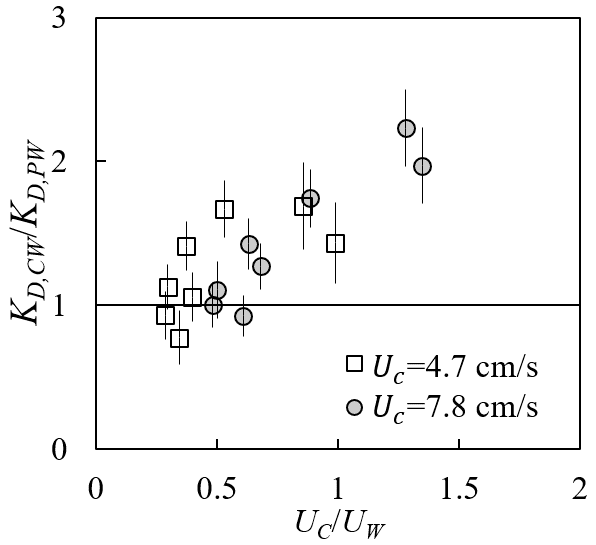
Figure 9Ratio of wave decay coefficients under combined conditions to pure wave conditions plotted against the ratio of current to wave velocity (adapted from Fig. 6a in Zhang and Nepf, 2021a).
Based on our laboratory measurements and theoretical analysis, we explain the different observed effects of current on wave dissipation as the result of the following competing mechanisms. First, consider the fact that the wave energy was only dissipated by plants; the time rate of energy dissipation scales with plant drag and canopy total velocity ED∼FDU. Adding current increases the total fluid velocity (Fig. 7) and thus the total plant force (Fig. 6), resulting in a greater wave energy dissipation compared to the same pure wave. Second, the influence of a current on wave dissipation is further modulated by the effect of plant resistance on the time-mean canopy flow structure (Fig. 7). In particular, the time-mean velocity within the canopy is significantly reduced compared to velocity upstream of the canopy at the same distance from the bed (P1 in Fig. 7). A reduction in time-mean velocity in the canopy, relative to the depth-averaged time-mean velocity, decreases the impact of currents on wave decay. Because the in-canopy current has a greater reduction for a denser canopy, the influence of a current on wave decay is diminished for a denser canopy relative to a sparser canopy. Third, a current changes the speed of wave energy propagation, i.e., the wave group velocity , which connects the time rate of wave energy dissipation to the spatial rate of wave energy dissipation (represented by KD). For the same |Uc| and plant drag (associated with the same ED), an opposing (following) current decreases (increases) Cg and generates larger (smaller) KD (spatial rate of amplitude decay).
For the experiments describe here, conducted in a finite length channel, the time-mean velocity was slightly negative for pure waves (Fig. 7b2) such that adding a small following current could lead to a decrease in the magnitude of time-mean velocity. A further increase in the current magnitude would increase the magnitude of time-mean and total velocity, which is why the present and previous studies (Hu et al., 2014; Yin et al., 2020) observed a reduction in KD only under a small following current, with a larger following current increasing KD compared to the same pure wave. The greater increase in KD under an opposing current than under a following current with the same magnitude, as observed in Hu et al. (2014) and Yin et al. (2020), can be explained by the effect of current direction on wave group velocity (the third mechanism above). The fact that the decrease in KD observed in highly flexible seagrass mimics (Paul et al., 2012) under a following current might be explained by the weaker increase in plant drag and canopy flow velocity (associated with a limited increase in the time rate of energy dissipation) and the decrease in KD due to an increase in wave group velocity Cg (the third mechanism above) compared to pure wave conditions. Specifically, increasing current led to a more pronated plant posture and decreased force on the flexible leaves compared to a leaf under the same pure wave (see Fig. 6 and Table 1 in Lei and Nepf, 2019a). Further, the time-mean velocity within the canopy height was smaller under combined currents and waves than for a pure current of the same magnitude (see Fig. 7a2 and c2), and the canopy time-mean velocity was further reduced by the decrease in canopy height due to plant reconfiguration because the deflection increased the plant solid volume fraction within the canopy and because in-canopy velocity decreases with an increasing degree of canopy submergence (Chen et al., 2013).
All instrument-measured data presented in this paper are available from Figshare (https://doi.org/10.6084/m9.figshare.24117144; Zhang and Nepf, 2023a). The repository includes the raw time series as well as phase-averaged and various statistical metrics (time mean, maximum, minimum) of force, surface displacement, and velocity. A “readme.pdf” file included in the repository provides additional data instructions. To enhance the accessibility of the data, we prepared the data in two formats, i.e., the SMCW.mat file and the SMCW.nc file, both of which are included in the Figshare link. The SMCW.mat can be directly imported into MATLAB and Python. The SMCW.nc file is a NetCDF file with metadata that can be accessed by C, C, Fortran, Python, and MATLAB. The plant motion recorded in the individual plant experiments can be found at https://doi.org/10.6084/m9.figshare.24117324 (Zhang and Nepf, 2023b). For each plant, a video with the same frame but including a ruler was included to give a scale of the plant motion.
5.1 Plant dynamic model validation
The plant motion videos, phase-resolving plant drag, free-surface displacement, and 3D velocity data can be used to validate phase-resolving plant dynamic models. The time-averaged force and velocity statistics can be used to validate phase-averaged plant drag models (as in Zhang and Nepf, 2021b, 2022). This dataset includes data not included in Zhang and Nepf (2021 and 2022) associated with strongly nonlinear waves, which reveal the nonlinear effects on plant motion and drag.
The measurements captured a phase lag between the plant force and wave motion (reflected by the free-surface displacement). The presence of a following current tended to increase the magnitude of this phase lag (Fig. 5). The dataset in Hu et al. (2021) also contained time lags between the wave (velocity) and force data (Fig. 5 in their paper). However, their wave and force data were not measured simultaneously, so the source of phase lag was unclear. Using a high-resolution synchronization method, Jacobsen et al. (2019) were able to capture the phase lag between the motion of a single flexible leaf and the fluid velocity, which filled an important knowledge gap in describing the physical cause of the observed phase lag. The present dataset can be used to deepen our understanding of the plant motion and force in response to waves with and without a current at high temporal resolution.
5.2 Flow structure within salt marsh meadow
The drag associated with a canopy has long been known to modify the vertical structure of current and wave velocity (Chen et al., 2013; Lowe et al., 2005; Zeller et al., 2015; Lei and Nepf, 2021), but few data have been reported under combined currents and waves. The present dataset directly compares the flow structure within a marsh canopy under a pure current, a pure wave, and their combination. Lowe et al. (2005) showed that a submerged canopy is more effective in reducing the time-mean velocity than the wave orbital velocity. They developed a two-layer model to predict the canopy wave orbital velocity without considering the influence of a current. Zeller et al. (2015) developed a prediction for the canopy total velocity under combined currents and waves. However, their model was only validated using five flow conditions in a rigid canopy. Further, previous studies of canopy velocity structure seldom compare the reduction of time-mean and wave orbital velocity using laboratory data measured under currents and waves acting alone and in combination. The present ME dataset provides high-resolution velocity profiles upstream of (single profile) and within (five lateral locations) a meadow under combined current and wave conditions (e.g., Fig. 7). The dataset covers water depth to plant height ratios from emergent to submerged and velocity ratios to 4.7. Measurements were also made using the same current and wave acting alone. This dataset can be utilized to study the interaction between currents and waves. In particular, the canopy time-mean velocity was reduced when waves were present (Fig. 7b2 and c2), suggesting that the waves enhanced the time-mean plant drag. The dataset can be used to validate theoretical and numerical models that predict canopy current and wave velocity.
5.3 Turbulent kinetic energy due to salt marsh
As shown in Fig. 7 and described in Sect. 3.2, the presence of marsh plants significantly enhanced turbulence intensity. For current over bare beds, turbulence is generated by spatial gradients in time-mean velocity (shear production), and the TKE is essentially uniform, except very close to the bed (circles in Fig. 7a1). However, when waves were presented, TKE was maximum near the free surface and decreased away from the surface (circles in Fig. 7b1 and c1), possibly due to time-mean shear introduced by the return current associated with wave conditions (circles in Fig. 7b3 and c3). Within the meadow, the TKE varied with position relative to individual plants. TKE was largest under combined current and wave conditions (compare the left column in Fig. 7), with turbulence peaks observed near the top of the canopy, associated with shear production by the time-mean current, and also within the canopy, associated with turbulence production in the wakes of individual plants (Fig. 7c1). This dataset can be used to develop and validate models to predict canopy turbulence (e.g., Xu and Nepf, 2020) and can be used in numerical models (e.g., Tang et al., 2021).
5.4 Wave decay over salt marsh meadow
The meadow experiments (MEs) measured the free-surface displacement along the length of the meadow with a horizontal interval of 10 and 15 cm, which included 18 to 26 points within one wave length (see Fig. C.1 in Zhang et al., 2022). The raw time series data can be utilized to analyze the transformation of wave shape, including wave skewness and wave asymmetry, over salt marshes. The wave shape is a crucial parameter when describing wave-driven sediment motion and is hence important for the study of coast stability within salt marsh regions.
The wave dissipation dataset presented here adds to the dataset reported in Hu et al. (2021), expanding the range of conditions. Specifically, Hu et al. (2021) reported wave decay data over rigid cylinders, while the present dataset provides wave decay over model plants with more realistic morphology and flexibility. The dataset can be applied to validate phase-averaged (e.g., Garzon et al., 2019a; Smith et al., 2016) and phase-resolving coastal models (e.g., Chen and Zou, 2019; Mattis et al., 2019) in predicting the wave energy reduction by salt marshes.
XZ designed the experiments, conducted the experiments, and collected the raw data. XZ prepared the paper, and HN reviewed and edited the paper.
The contact author has declared that none of the authors has any competing interests.
Publisher's note: Copernicus Publications remains neutral with regard to jurisdictional claims made in the text, published maps, institutional affiliations, or any other geographical representation in this paper. While Copernicus Publications makes every effort to include appropriate place names, the final responsibility lies with the authors.
We thank Jiarui Lei for his guidance with the experimental equipment.
This research has been supported by the National Key Research and Development Program of China (grant no. 2022YFE0136700), the China Scholarship Council, and the National Science Foundation (grant no. EAR 1659923).
This paper was edited by Alberto Ribotti and reviewed by Francesco Paladini de Mendoza and one anonymous referee.
Barbier, E. B., Hacker, S. D., Kennedy, C., Koch, E. W., Stier, A. C., and Silliman, B. R.: The value of estuarine and coastal ecosystem services, Ecol. Monogr., 81, 169–193, https://doi.org/10.1890/10-1510.1, 2011.
Boesch, D. F. and Turner, R. E.: Dependence of fishery species on salt marshes: The role of food and refuge, Estuaries, 7, 460–468, https://doi.org/10.2307/1351627, 1984.
Borges, F. O., Santos, C. P., Paula, J. R., Mateos-Naranjo, E., Redondo-Gomez, S., Adams, J. B., Caçador, I., Fonseca, V. F., Reis-Santos, P., Duarte, B., and Rosa, R.: Invasion and Extirpation Potential of Native and Invasive Spartina Species Under Climate Change, Front. Mar. Sci., 8, 696333, https://doi.org/10.3389/fmars.2021.696333, 2021.
Chen, H. and Zou, Q.: Eulerian–Lagrangian flow-vegetation interaction model using immersed boundary method and OpenFOAM, Adv. Water Resour., 126, 176–192, https://doi.org/10.1016/j.advwatres.2019.02.006, 2019.
Chen, Z., Jiang, C., and Nepf, H.: Flow adjustment at the leading edge of a submerged aquatic canopy, Water Resour. Res., 49, 5537–5551, https://doi.org/10.1002/wrcr.20403, 2013.
Elschot, K., Bouma, T. J., Temmerman, S., and Bakker, J. P.: Effects of long-term grazing on sediment deposition and salt-marsh accretion rates, Estuarine, Coast. Shelf Sci., 133, 109–115, https://doi.org/10.1016/j.ecss.2013.08.021, 2013.
Garzon, J. L., Miesse, T., and Ferreira, C. M.: Field-based numerical model investigation of wave propagation across marshes in the Chesapeake Bay under storm conditions, Coast. Eng., 146, 32–46, https://doi.org/10.1016/j.coastaleng.2018.11.001, 2019a.
Garzon, J. L., Maza, M., Ferreira, C. M., Lara, J. L., and Losada, I. J.: Wave attenuation by Spartina saltmarshes in the Chesapeake Bay under storm surge conditions, J. Geophys. Res.-Oceans, 124, 5220–5243, https://doi.org/10.1029/2018JC014865, 2019b.
Gosselin, F., De Langre, E., and Machado-Almeida, B. A.: Drag reduction of flexible plates by reconfiguration, J. Fluid Mech., 650, 319–341, https://doi.org/10.1017/S0022112009993673, 2010.
Harder, D. L., Speck, O., Hurd, C. L., and Speck, T.: Reconfiguration as a prerequisite for survival in highly unstable flow-dominated habitats, J. Plant Growth Regul., 23, 98–107, https://doi.org/10.1007/s00344-004-0043-1, 2004.
Hu, Z., Suzuki, T., Zitman, T., Uittewaal, W., and Stive, M.: Laboratory study on wave dissipation by vegetation in combined current–wave flow, Coast. Eng., 88, 131–142, https://doi.org/10.1016/j.coastaleng.2014.02.009, 2014.
Hu, Z., Lian, S., Wei, H., Li, Y., Stive, M., and Suzuki, T.: Laboratory data on wave propagation through vegetation with following and opposing currents, Earth Syst. Sci. Data, 13, 4987–4999, https://doi.org/10.5194/essd-13-4987-2021, 2021.
Huai, W., Li, S., Katul, G. G., Liu, M., and Yang, Z.: Flow dynamics and sediment transport in vegetated rivers: A review, J. Hydrodyn., 33, 400–420, https://doi.org/10.1007/s42241-021-0043-7, 2021.
Jacobsen, N. G., Bakker, W., Uijttewaal, W. S. J., and Uittenbogaard, R.: Experimental investigation of the wave-induced motion of and force distribution along a flexible stem, J. Fluid Mech., 880, 1036–1069, https://doi.org/10.1017/jfm.2019.739, 2019.
Jalonen, J. and Järvelä, J.: Impact of tree scale on drag: Experiments in a towing tank, in: Proceedings of 2013 IAHE world Congress, vol. 1, London, UK, Chengdu: Taylor & Francis, p. 12, 2013.
Keulegan, G. H. and Carpenter, L. H.: Forces on cylinders and plates in an oscillating fluid, J. Res. Nat. Bur. Stan., 60, 423–440, https://doi.org/10.6028/jres.060.043, 1958.
Knutson, P. L., Brochu, R. A., Seeling, W. N., and Margaret, I.: Wave damping in Spartina alterniflora marsh, Wetlands, 2, 87–104, 1982.
Lei, J. and Nepf, H.: Blade dynamics in combined waves and current, J. Fluid. Struct., 87, 137–149, https://doi.org/10.1016/j.jfluidstructs.2019.03.020, 2019a.
Lei, J. and Nepf, H.: Wave damping by flexible vegetation: Connecting individual blade dynamics to the meadow scale, Coast. Eng., 147, 138–148, https://doi.org/10.1016/j.coastaleng.2019.01.008, 2019b.
Lei, J. and Nepf, H.: Evolution of flow velocity from the leading edge of 2-D and 3-D submerged canopies, J. Fluid Mech., 916, A36, https://doi.org/10.1017/jfm.2021.197, 2021.
Li, C. W. and Yan, K.: Numerical investigation of wave–current–vegetation interaction, J. Hydraul. Eng., 133, 794–803, https://doi.org/10.1061/(ASCE)0733-9429(2007)133:7(794), 2007.
Losada, I. J., Maza, M., and Lara, J. L.: A new formulation for vegetation-induced damping under combined waves and currents, Coast. Eng., 107, 1–13, https://doi.org/10.1016/j.coastaleng.2015.09.011, 2016.
Lowe, R. J., Koseff, J. R., and Monismith, S. G.: Oscillatory flow through submerged canopies: 1. Velocity structure, J. Geophys. Res.-Oceans, 110, C10016, https://doi.org/10.1029/2004JC002788, 2005.
Luhar, M. and Nepf, H. M.: Flow-induced reconfiguration of buoyant and flexible aquatic vegetation, Limnol. Oceanogr., 56, 2003–2017, https://doi.org/10.4319/lo.2011.56.6.2003, 2011.
Luhar, M. and Nepf, H. M.: Wave induced dynamics of flexible blades, J. Fluid. Struct., 61, 20–41, https://doi.org/10.1016/j.jfluidstructs.2015.11.007, 2016.
Mattis, S. A., Kees, C. E., Wei, M. V., Dimakopoulos, A., and Dawson, C. N.: Computational model for wave attenuation by flexible vegetation, J. Waterway, Port, Coastal, Ocean Eng., 145, 04018033, https://doi.org/10.1061/(ASCE)WW.1943-5460.0000487, 2019.
Maza, M., Lara, J. L., Losada, I. J., Ondiviela, B., Trinogga, J., and Bouma, T. J.: Large-scale 3-D experiments of wave and current interaction with real vegetation. Part 2: Experimental analysis, Coast. Eng., 106, 73–86, https://doi.org/10.1016/j.coastaleng.2015.09.010, 2015.
Monismith, S. G.: Stokes drift: theory and experiments, J. Fluid Mech., 884, F1, https://doi.org/10.1017/jfm.2019.891, 2020.
Morison, J. R., Johnson, J. W., and Schaaf, S. A.: The force exerted by surface waves on piles, J. Petrol. Technol., 2, 149–154, https://doi.org/10.2118/950149-G, 1950.
Mullarney, J. C. and Henderson, S. M.: Wave-forced motion of submerged single-stem vegetation, J. Geophys. Res., 115, C12061, https://doi.org/10.1029/2010JC006448, 2010.
Nepf, H. M.: Flow and transport in regions with aquatic vegetation, Annu. Rev. Fluid Mech., 44, 123–142, https://doi.org/10.1146/annurev-fluid-120710-101048, 2012.
Paul, M., Bouma, T., and Amos, C.: Wave attenuation by submerged vegetation: combining the effect of organism traits and tidal current, Mar. Ecol. Prog. Ser., 444, 31–41, https://doi.org/10.3354/meps09489, 2012.
Pidgeon, E.: Carbon sequestration by coastal marine habitats: Important missing sinks, in: The Management of Natural Coastal Carbon Sinks, IUCN, 2009.
Schoutens, K., Heuner, M., Minden, V., Schulte Ostermann, T., Silinski, A., Belliard, J.-P., and Temmerman, S.: How effective are tidal marshes as nature-based shoreline protection throughout seasons, Limnol. Oceanogr., 64, 1750–1762, https://doi.org/10.1002/lno.11149, 2019.
Schoutens, K., Heuner, M., Fuchs, E., Minden, V., Schulte-Ostermann, T., Belliard, J.-P., Bouma, T. J., and Temmerman, S.: Nature-based shoreline protection by tidal marsh plants depends on trade-offs between avoidance and attenuation of hydrodynamic forces, Estuar. Coast. Shelf Sci., 236, 106645, https://doi.org/10.1016/j.ecss.2020.106645, 2020.
Schoutens, K., Luys, P., Heuner, M., Fuchs, E., Minden, V., Schulte Ostermann, T., Bouma, T., Van Belzen, J., and Temmerman, S.: Traits of tidal marsh plants determine survival and growth response to hydrodynamic forcing: implications for nature-based shoreline protection, Mar. Ecol. Prog. Ser., 693, 107–124, https://doi.org/10.3354/meps14091, 2022.
Schutten, J. and Davy, A. J.: Predicting the hydraulic forces on submerged macrophytes from current velocity, biomass and morphology, Oecologia, 123, 445–452, https://doi.org/10.1007/s004420000348, 2000.
Smith, J. M., Bryant, M. A., and Wamsley, T. V.: Wetland buffers: numerical modeling of wave dissipation by vegetation, Earth Surf. Proc. Land., 41, 847–854, https://doi.org/10.1002/esp.3904, 2016.
Tang, X., Lin, P., Liu, P. L. -F., and Liu, X.: Numerical and experimental studies of turbulence in vegetated open-channel flows, Environ. Fluid Mech., 21, 1137–1163, https://doi.org/10.1007/s10652-021-09812-7, 2021.
van Veelen, T. J., Fairchild, T. P., Reeve, D. E., and Karunarathna, H.: Experimental study on vegetation flexibility as control parameter for wave damping and velocity structure, Coast. Eng., 157, 103648, https://doi.org/10.1016/j.coastaleng.2020.103648, 2020.
Vuik, V., Jonkman, S. N., Borsje, B. W., and Suzuki, T.: Nature-based flood protection: The efficiency of vegetated foreshores for reducing wave loads on coastal dikes, Coast. Eng., 116, 42–56, https://doi.org/10.1016/j.coastaleng.2016.06.001, 2016.
Whittaker, P., Wilson, C., Aberle, J., Rauch, H. P., and Xavier, P.: A drag force model to incorporate the reconfiguration of full-scale riparian trees under hydrodynamic loading, J. Hydraul. Res., 51, 569–580, https://doi.org/10.1080/00221686.2013.822936, 2013.
Xu, Y. and Nepf, H.: Measured and predicted turbulent kinetic energy in flow through emergent vegetation with real plant morphology, Water Resour. Res., 56, e2020WR027892, https://doi.org/10.1029/2020WR027892, 2020.
Yin, Z., Wang, Y., Liu, Y., and Zou, W.: Wave attenuation by rigid emergent vegetation under combined wave and current flows, Ocean Eng., 213, 107632, https://doi.org/10.1016/j.oceaneng.2020.107632, 2020.
Ysebaert, T., Yang, S., Zhang, L., He, Q., Bouma, T. J., and Herman, P. M. J.: Wave attenuation by two contrasting ecosystem engineering salt marsh macrophytes in the intertidal pioneer zone, Wetlands, 31, 1043–1054, https://doi.org/10.1007/s13157-011-0240-1, 2011.
Zeller, R. B., Zarama, F. J., Weitzman, J. S., and Koseff, J. R.: A simple and practical model for combined wave-current canopy flows, J. Fluid Mech., 767, 842–880, https://doi.org/10.1017/jfm.2015.59, 2015.
Zhang, X. and Nepf, H.: Flow-induced reconfiguration of aquatic plants, including the impact of leaf sheltering, Limnol. Oceanogr., 65, 2697–2712, https://doi.org/10.1002/lno.11542, 2020.
Zhang, X. and Nepf, H.: Wave damping by flexible marsh plants influenced by current, Phys. Rev. Fluids, 6, 100502, https://doi.org/10.1103/PhysRevFluids.6.100502, 2021a.
Zhang, X. and Nepf, H.: Wave-induced reconfiguration of and drag on marsh plants, J. Fluid. Struct., 100, 103192, https://doi.org/10.1016/j.jfluidstructs.2020.103192, 2021b.
Zhang, X. and Nepf, H.: Reconfiguration of and drag on marsh plants in combined waves and current, J. Fluid. Struct., 110, 103539, https://doi.org/10.1016/j.jfluidstructs.2022.103539, 2022.
Zhang, X. and Nepf, H.: A dataset on the hydrodynamic force on individual salt marsh plants and the flow structure and wave dissipation over a meadow of plants under waves with and without current, figshare [data set], https://doi.org/10.6084/m9.figshare.24117144, 2023a.
Zhang, X. and Nepf, H.: Salt marsh dynamic motion videos under waves with and without current, figshare [video], https://doi.org/10.6084/m9.figshare.24117324, 2023b.
Zhang, X., Lin, P., Gong, Z., Li, B., and Chen, X.: Wave attenuation by Spartina alterniflora under macro-tidal and storm surge conditions, Wetlands, 40, 2151–2162, https://doi.org/10.1007/s13157-020-01346-w, 2020.
Zhang, X., Lin, P., and Nepf, H.: A simple wave damping model for flexible marsh plants, Limnol. Oceanogr., 66, 4182–4196, https://doi.org/10.1002/lno.11952, 2021.
Zhang, X., Lin, P., and Nepf, H.: A wave damping model for flexible marsh plants with leaves considering linear to weakly nonlinear wave conditions, Coast. Eng., 175, 104124, https://doi.org/10.1016/j.coastaleng.2022.104124, 2022.
Zhang, X., Zhao, C., and Nepf, H.: A simple prediction of time-mean and wave 2 orbital velocities in submerged canopy, J. Fluid Mech., 0, A1, https://doi.org/10.1017/jfm.2024.61, 2024.
Zhao, C., Tang, J., and Shen, Y.: Experimental study on solitary wave attenuation by emerged vegetation in currents, Ocean Eng., 220, 108414, https://doi.org/10.1016/j.oceaneng.2020.108414, 2020.
Zhu, L., Zou, Q., Huguenard, K., and Fredriksson, D. W.: Mechanisms for the asymmetric motion of submerged aquatic vegetation in waves: A consistent-mass cable model, J. Geophys. Res.-Oceans, 125, e2019JC015517, https://doi.org/10.1029/2019JC015517, 2020.
Zhu, L., Chen, Q., Ding, Y., Jafari, N., Wang, H., and Johnson, B. D.: Towards a unified drag coefficient formula for quantifying wave energy reduction by salt marshes, Coast. Eng., 180, 104256, https://doi.org/10.1016/j.coastaleng.2022.104256, 2023.