the Creative Commons Attribution 4.0 License.
the Creative Commons Attribution 4.0 License.
 | 04 Jan 2023
Version 2 of the global catalogue of large anthropogenic and volcanic SO2 sources and emissions derived from satellite measurements
Vitali E. Fioletov
Chris A. McLinden
Debora Griffin
Ihab Abboud
Nickolay Krotkov
Peter J. T. Leonard
Joanna Joiner
Nicolas Theys
Simon Carn
Sulfur dioxide (SO2) measurements from the Ozone Monitoring Instrument (OMI), Ozone Mapping and Profiler Suite (OMPS), and TROPOspheric Monitoring Instrument (TROPOMI) satellite spectrometers were used to update and extend the previously developed global catalogue of large SO2 emission sources. This version 2 of the global catalogue covers the period of 2005–2021 and includes a total of 759 continuously emitting point sources releasing from about 10 kt yr−1 to more than 4000 kt yr−1 of SO2, that have been identified and grouped by country and primary source origin: volcanoes (106 sources); power plants (477); smelters (74); and sources related to the oil and gas industry (102). There are several major improvements compared to the original catalogue: it combines emissions estimates from three satellite instruments instead of just OMI, uses a new version 2 of the OMI and OMPS SO2 dataset, and updated consistent site-specific air mass factors (AMFs) are used to calculate SO2 vertical column densities (VCDs). The newest TROPOMI SO2 data processed with the Covariance-Based Retrieval Algorithm (COBRA), used in the catalogue, can detect sources with emissions as low as 8 kt yr−1 (in 2018–2021) compared to the 30 kt yr−1 limit for OMI. In general, there is an overall agreement within ±12 % in total emissions estimated from the three satellite instruments for large regions. For individual emission sources, the spread is larger: the annual emissions estimated from OMI and TROPOMI agree within ±13 % in 50 % of cases and within ±28 % in 90 % of cases. The version 2 catalogue emissions were calculated as a weighted average of emission estimates from the three satellite instruments using an inverse-variance weighting method. OMI, OMPS, and TROPOMI data contribute 7 %, 5 %, and 88 % to the average, respectively, for small (<30 kt yr−1) sources and 33 %, 20 %, and 47 %, respectively, for large (>300 kt yr−1) sources. The catalogue data show an approximate 50 % decline in global SO2 emissions between 2005 and 2021, although emissions were relatively stable during the last 3 years. The version 2 of the global catalogue has been posted at the NASA global SO2 monitoring website (https://doi.org/10.5067/MEASURES/SO2/DATA406, Fioletov et al., 2022).
- Article
(4292 KB) - Full-text XML
- BibTeX
- EndNote


Sulfur dioxide (SO2) plays an important role in atmospheric processes that impact the environment, health, atmospheric chemistry, and climate (Hansell and Oppenheimer, 2010; Robock, 2000). It poses a direct hazard to public health (Longo et al., 2010; Pope and Dockery, 2006) and, therefore, is a designated criteria air pollutant in many countries. SO2 also leads to acid deposition that affects terrestrial ecosystems (Dentener et al., 2006; Hutchinson and Whitby, 1977; Vet et al., 2014). Coal-burning power plants, oil refineries, and smelters are the primary anthropogenic emitters of SO2 (Klimont et al., 2013; Smith et al., 2011), while volcanoes are the primary natural source of SO2 (Carn et al., 2017; Oppenheimer et al., 2011).
Due to strong absorption of UV radiation, it is possible to retrieve SO2 vertical column density (VCD) from satellite measurements in the UV part of the spectrum. Such retrievals were first performed using measurements by the Total Ozone Mapping Spectrometer (TOMS) and the Solar Backscattered Ultraviolet (SBUV) instruments on Nimbus 7 satellite after a large injection of volcanic SO2 from the El Chichón eruption in 1982 (Krueger, 1983; McPeters et al., 1984). Industrial emission sources were first detected from space using measurements by the Global Ozone Monitoring Experiment (GOME) on the European Remote Sensing satellite 2 (ERS-2) (Eisinger and Burrows, 1998; Khokhar et al., 2008). Measurements by the two subsequent satellite instruments, the SCanning Imaging Absorption spectroMeter for Atmospheric CHartographY (SCIAMACHY), 2002–2012 on the ENVISAT satellite (Bovensmann et al., 1999), and the Global Ozone Monitoring Experiment-2 (GOME 2) instrument, 2006–present, on MetOp-A (Callies et al., 2000), were used to detect and monitor emissions from a few dozen sources (Fioletov et al., 2013). A new era of satellite SO2 measurements started with the launch of the Dutch–Finnish Ozone Monitoring Instrument (OMI) (Levelt et al., 2018, 2006) on NASA's Earth Observing System (EOS) – Chemistry Aura spacecraft (Schoeberl et al., 2006) in 2004. At that time, OMI had the highest spatial resolution (up to 13×24 km2) of any UV satellite instrument and was able to provide daily, nearly global maps of SO2 VCDs, permitting the analysis of long-term trends in SO2 emissions on a regional and global scale (Krotkov et al., 2016).
A catalogue of large SO2 sources and their emissions estimated from OMI measurements was introduced 6 years ago (Fioletov et al., 2016; McLinden et al., 2016). At that time, the catalogue included 491 continuously emitting point sources, of which 76 were volcanoes, 297 were powerplants, 53 were smelters, and 65 were sources related to the oil and gas industry. The catalogue was updated annually, and additional sources were added with the most recent version of the catalogue including 588 sources and available from the NASA global SO2 monitoring website at https://so2.gsfc.nasa.gov/measures.html (last access: 7 November 2022). The catalogue was used to update and improve available bottom-up emissions inventories used in air quality and climate models (Liu et al., 2018; Ukhov et al., 2020), to evaluate the efficiency of industrial clean technology solutions in reducing air pollution (Ialongo et al., 2018; McLinden et al., 2020) and to monitor changes in SO2 emissions on a large scale (Li et al., 2017). The catalogue estimates for volcanic sources were used to analyse volcanic SO2 emissions (Carn et al., 2017) and, using SO2 as a proxy, to estimate volcanic carbon dioxide (CO2) fluxes (Fischer et al., 2019). The approach to catalogue large emission point sources was later applied to satellite measurements of ammonia (NH3) (Van Damme et al., 2018; Dammers et al., 2019) and nitrogen dioxide (NO2) (Beirle et al., 2021).
There have been several important developments since publication of the original SO2 catalogue. Satellite SO2 measurements by the Ozone Mapping and Profiler Suite (OMPS) (Zhang et al., 2017) on the NASA–NOAA Suomi National Polar-orbiting Partnership (SNPP) spacecraft (Flynn et al., 2014; Seftor et al., 2014) and by the TROPOspheric Monitoring Instrument (TROPOMI) (Theys et al., 2017) on the ESA Copernicus Sentinel-5 Precursor (S-5P) spacecraft (Veefkind et al., 2012) became available starting in 2012 and 2018, respectively. Their measurements are suitable for SO2 emissions estimates and can provide additional inputs for the SO2 catalogue (Fioletov et al., 2020; Theys et al., 2021; Zhang et al., 2017). A newer European Centre for Medium-Range Weather Forecasts (ECMWF) Reanalysis v5 (ERA5) reanalysis version (C3S, 2017) provides wind data with a higher spatial and temporal resolution than the ERA-Interim reanalysis (Dee et al., 2011) used in the original SO2 catalogue. A new version 2.0 of the SO2 retrieval algorithm was developed for OMI and OMPS SO2 retrievals (Li et al., 2020c), and the entire OMI and OMPS data records were reprocessed in 2020–2021.
After the release of the version 2.0 OMI SO2 product in 2020, production of the previous version 1.2 used in the original catalogue was discontinued, so it was necessary to recalculate the SO2 emissions using version 2.0, and that was done in this study. There were also some additional improvements in this updated version of the catalogue, and we decided to call it version 2. The original catalogue was based on OMI SO2 data that have a source detection limit of 30–40 kt yr−1 (Fioletov et al., 2015, 2016), whereas the newest TROPOMI SO2 dataset processed with the Covariance-Based Retrieval Algorithm (COBRA) can detect sources with emissions as low as 8 kt yr−1 (Theys et al., 2021), and therefore more sources can be “seen”. In this study, we discuss the implications of the change in OMI SO2 data product versions as well as further changes introduced in the catalogue. Note that the SO2 emission estimation algorithm used here is identical to that in the original study (Fioletov et al., 2016) to assure the continuity of the old and new emissions estimates. For this reason, we do not use a newer version of the emission estimation algorithm (Fioletov et al., 2017; McLinden et al., 2020) that can better handle multiple emission sources in close proximity, which we plan to utilise in subsequent versions of the catalogue.
This article introduces a new version 2 of the global catalogue of large SO2 sources and their emissions. It is organised as follows: the datasets and the emission calculation algorithm are described in Sect. 2. Section 3 discusses the differences between emissions estimated from different versions of the OMI algorithm and SO2 emissions estimates from different satellite instruments. An overview of the estimated emissions is given in Sect. 4. Section 5 concludes the study.
VCDs measured by three hyperspectral “push broom” UV satellite sensors, OMI, OMPS, and TROPOMI, were used in this study. SO2 VCDs are given as in Dobson units (DU, molec cm−2) and the estimated annual emissions are in metric kilotonnes of SO2 per year (kt yr−1).
2.1 OMI and OMPS data
OMI was launched on NASA's EOS Aura satellite on 15 July 2004 (Schoeberl et al., 2006). Aura is in a sun-synchronous polar orbit and crosses the Equator at about 13:45 LT. OMI is a nadir-viewing UV-visible spectrometer that initially provided daily global coverage with a resolution of up to 13 km×24 km at nadir (de Graaf et al., 2016). The OMI detector has 60 cross-track positions, however about half of its pixels have been affected by a field-of-view blockage and stray light (the so-called “row anomaly”) after 2007 (Levelt et al., 2018). As in the original catalogue, the first 10 and last 10 cross-track positions were excluded from the analysis to limit the across-track pixel width from 24 km to about 40 km.
The OMPS Nadir Mapper, a UV spectrometer on board the NASA–NOAA Suomi NPP satellite, was launched in October 2011. The OMPS detector has 36 cross-track positions and a nadir resolution of 50 km×50 km. Similar to the OMI data analysis, the first two and last two OMPS cross-track positions were excluded. Suomi NPP is also in a polar orbit and crosses the Equator at about the same time as Aura – at about 13:30 LT.
The original catalogue was based on the OMI SO2 VCD data product calculated using algorithm version 1.2 that is based on principal component analysis (PCA) of OMI-measured radiances (Li et al., 2013). In this study, we used the version 2 OMI and OMPS PCA SO2 data (Li et al., 2020c). In the version 2, for each scene there are six different estimates of the SO2 VCD in DU obtained by making different assumptions about the vertical distribution of SO2. Users interested in anthropogenic SO2 pollution are advised to pick VCDs produced by spectral fitting using SO2 Jacobians that more accurately account for the effects of sun–satellite geometry, clouds, O3, and surface reflectivity on OMI (and OMPS) sensitivity, and use updated a priori SO2 vertical profiles from chemical transport model (CTM) simulations (i.e. the ColumnAmountSO2 field in the OMI and OMPS datasets, Li et al., 2020a, b). In addition, version 2 also provides an estimate of the slant column density (SCD) produced by spectral fitting using SO2 cross sections (i.e. SlantColumnAmountSO2 field). When converted to VCD using a site-specific air mass factor () (McLinden et al., 2014), this dataset can be used as a continuity product for the previous version. The differences between the emissions estimates using the two approaches are discussed in Sect. 3.
OMI data for the period 2005–2021 and OMPS data for the period 2012–2021 were analysed. Only Level-2 clear-sky data, defined as having a cloud radiance fraction of less than 0.3, were used for the catalogue. Measurements at solar zenith angles (SZAs) more than 70∘ as well as measurements taken over snow or ice were excluded. As in the original catalogue, the retrieved SO2 VCDs correspond to 1 km thick plumes located near the surface as we focus on anthropogenic and passive volcanic degassing sources. Typical standard deviations of the individual OMI VCDs over background areas are between 0.6 DU in the tropics and 1 DU at high latitudes. The same values for OMPS are 0.3–0.4 DU (Fioletov et al., 2020).
2.2 TROPOMI data
TROPOMI was launched on the ESA Copernicus S5-P satellite on 13 October 2017 (Veefkind et al., 2012). The instrument consists of UV–Vis–NIR spectrometers and SO2 can be retrieved from the UV part of the measured spectra. The TROPOMI detector has 450 cross-track positions, however the first and last 20 of them were excluded from our analysis due to a relatively high noise level (Fioletov et al., 2020). The spatial resolution for the centre of the swath was originally 3.5 km×7 km (along track) and it was reduced to 3.5 km×5.5 km after 6 August 2019.
The original operational TROPOMI differential optical absorption spectroscopy (DOAS)-based algorithm (Theys et al., 2017) produced SO2 data with high spatial resolution that made it possible to study SO2 emission sources in greater detail and detect sources that previously were below the sensitivity limits of OMI and OMPS (Fioletov et al., 2020). However, the noise level was relatively high and the data had large-scale variable biases (Fioletov et al., 2020; Theys et al., 2021). These issues were largely resolved by a new Covariance-Based Retrieval Algorithm (COBRA) (Theys et al., 2021). Moreover, COBRA even demonstrated lower uncertainties than the PCA-based algorithm when the same set of samples was processed by the two algorithms (Theys et al., 2021). It is expected that COBRA will replace the present operational SO2 algorithm in near future. In this study, Level-2 COBRA data for the period from 1 April 2018 to 31 December 2021 were used. As for OMI and OMPS, clear-sky-only data, defined as having a cloud radiance fraction of less than 0.3, were used for the catalogue. Measurements at SZAs larger than 70∘ as well as measurements taken over snow or ice were excluded. The standard deviations of individual TROPOMI SO2 VCD were between 1 DU in the tropics and 1.5 DU at high latitudes for the original operational algorithm (Fioletov et al., 2020) and 50 % lower for the COBRA version (Theys et al., 2021), i.e. comparable to or even lower than the OMI noise despite a 16 times smaller TROPOMI pixel area. Note that there is a 22 % systematic difference between retrieved OMI/OMPS and TROPOMI SCD caused by the difference in SO2 cross section temperature (203 K for TROPOMI vs. 293 K for OMI/OMPS), as discussed by Theys et al. (2017, their Fig. 6). To account for it, the TROPOMI SO2 VCD values calculated in this study were increased by 22 % (Fioletov et al., 2020; Theys et al., 2017).
2.3 Other datasets
The emission estimation algorithm requires information on the wind speed and direction that are obtained from ECMWF reanalysis data. The most recent ERA5 wind data (C3S, 2017) provided U- and V- (west–east and south–north, respectively) wind-speed components with hourly temporal resolution on a 0.25∘ by 0.25∘ grid. They were grouped into 1 km-thick layers and the mean wind speed and direction were calculated for each level as it was done for the original catalogue. The reanalysis wind data for regular pressure levels were linearly interpolated to overpass time and to the location of the centre of each satellite sensor pixel. The winds for the layer that corresponds to the height of a source were used by the algorithm. Please note that in ERA5 for elevated locations, the wind data at levels below the surface pressure layer are simply duplicates of the winds at the lowest pressure available.
As in the original catalogue, measurements with snow on the ground were excluded from the analysis. The Interactive Multisensor Snow and Ice Mapping System (IMS) data were used as a source of the snow cover information (Helfrich et al., 2007).
3.1 The fitting algorithm
As mentioned in the Introduction, this study employs the same fitting algorithm as the original catalogue to estimate the total average SO2 mass near the source and derive emissions assuming a constant lifetime. The algorithm is described in detail in our previous studies (Fioletov et al., 2015, 2016) and we briefly review its key features here.
The algorithm fits the plume from an emission point source by a fitting function and then this fit is used to calculate the total SO2 mass (α) near the source and the emission strength , where τ is a constant parameter that represents the SO2 lifetime (or decay time). The fitting function is an exponentially modified Gaussian (EMG) function (Beirle et al., 2014; Fioletov et al., 2015; de Foy et al., 2015) along the wind direction and a Gaussian function with plume width ω across the wind direction. The wind direction and speed are taken from the ERA5 reanalysis data. The algorithm uses two prescribed constant parameters (τ and ω). One unknown parameter, α, is estimated from the fit. All satellite pixels within a rectangular area along the wind direction collected for 1 year (if annual emissions are estimated) are used for the fitting. The rectangular fitting area extends ±L km across the wind direction, L km in the upwind direction and 3⋅L km in the downwind direction, where the parameter L depends on the emission strength on the source: from 30 km for sources under 100 kt yr−1 to 90 km for sources greater than 1000 kt yr−1.
The values of the prescribed parameters τ=6 h, and ω=20, 25, and 15 km for OMI, OMPS, and TROPOMI, respectively, are chosen as in the previous studies (Fioletov et al., 2020, 2016). Note, that the estimated emissions are not very sensitive to small uncertainties in the plume width: e.g. a 5 km change (from 20 to 25 km) in the ω value for OMI produces only a 10 %–15 % change in the estimated emissions. As in previous studies, only pixels with associated wind speeds between 0.5 and 45 km h−1 are used. Also, as in the original catalogue, high transient volcanic SO2 VCDs were screened out by setting an upper limit on SO2 VCDs: days when some pixels in the fitting area exceeded such limits were excluded from the analysis. These limits depend on the source emission strength (obtained from preliminary estimates).
There is a potential problem of overestimating emissions in the case of multiple sources in an area. Previous analysis of OMI data demonstrated that sources can be distinguished if the distance between them is greater than about 80 km but emissions can be overestimated if this distance is less than 50 km, although these limits would also depend on the emission strength and prevailing wind direction (Fioletov et al., 2016). In some cases, however, we found that emissions from two sources can be clearly separated even if they are only 40 km apart. These limits should be even lower for TROPOMI data with its much smaller pixel size. For this reason, we included 20 sources in the catalogue that are only 35–40 km apart but appear as isolated “hotspots” on TROPOMI SO2 maps. For each source, we also added information on the distance to the nearest other source in the catalogue, so the users can do their own screening. In addition, to avoid “double counting” for regional emission estimates, some sources were not included in the catalogue if there is a source nearby that is already in the catalogue. This typically occurs in some regions of the US and China.
Based on the uncertainty budget of estimated emissions (Fioletov et al., 2016, their Table 1), the overall uncertainty is about 50 %. The main contributors are uncertainties in AMFs, lifetime, and plume widths that affect emissions as scaling factors, i.e. affect the absolute values but not so much relative changes of the estimated emissions. The SO2 emission detection limit (defined as a level where the estimated annual emission is 3 times larger that its standard error) is about 8 kt yr−1 for TROPOMI and 30–40 kt yr−1 for OMI for the first years of operation and even higher for OMPS (Theys et al., 2021).
3.2 OMI/MPS version 2
Version 2 OMI (and OMPS) VCDs are different from the previous version 1.2 that was used in the original catalogue. The differences are discussed first before we analyse the estimated emissions. The original OMI retrieval algorithm estimated SO2 slant column density (SCD) first. The SCD was then converted to VCD by applying a constant AMF=0.36 that was optimised for anthropogenic pollution in the eastern US in summer (Krotkov et al., 2008, 2006; Li et al., 2013). In the original SO2 catalogue, we replaced that with source specific AMFs, which were pre-calculated using site-specific elevation, climatological aerosols, and surface reflectance (albedo) (McLinden et al., 2014). The same AMFs from the original catalogue were also applied to TROPOMI COBRA SCDs to calculate consistent VCDs and emissions (Theys et al., 2021). Although version 2 of OMI and OMPS data provide VCDs for each pixel (i.e. ColumnAmountSO2), we do not use them here to ensure consistency between the original and the new versions of the catalogue. The same is also true for TROPOMI COBRA SO2 data.
To illustrate the differences between SO2 VCDs calculated using different AMFs, Fig. 1 shows examples of SO2 emissions from the original catalogue, emissions estimated from OMI version 2 SCDs converted to VCDs using the same site-specific AMFs as in the original catalogue, and emissions estimated using version 2 OMI VCD data (i.e. ColumnAmountSO2). We also included TROPOMI data that are discussed in Sect. 3.4. Figure 1 (top row) shows estimated emissions from two Mexican sites, Tula and Cantarell, located at the same latitude and 7∘ apart in longitude. Emissions from Tula are well known (de Foy et al., 2009) and included in the CTM used to calculate a priori SO2 profiles in the OMI version 2 ColumnAmountSO2 product. In contrast, Cantarell is an oil field in the Gulf of Mexico (Fioletov et al., 2013; Villasenor et al., 2003) and its SO2 emissions (mostly from flaring) may not be properly accounted for in the CTM. As a result, the a priori SO2 vertical profile used in the Jacobian calculations assumes that the SO2 is in the free troposphere rather than near the surface, and therefore overestimates the OMI sensitivity and leads to underestimation of emissions. Another example of the difference between emission estimates from different datasets that is related to the source altitude is shown in Fig. 1 (bottom row). The two sources from the Middle East are at the same latitude, 5∘ apart in the longitude, but at different elevations.
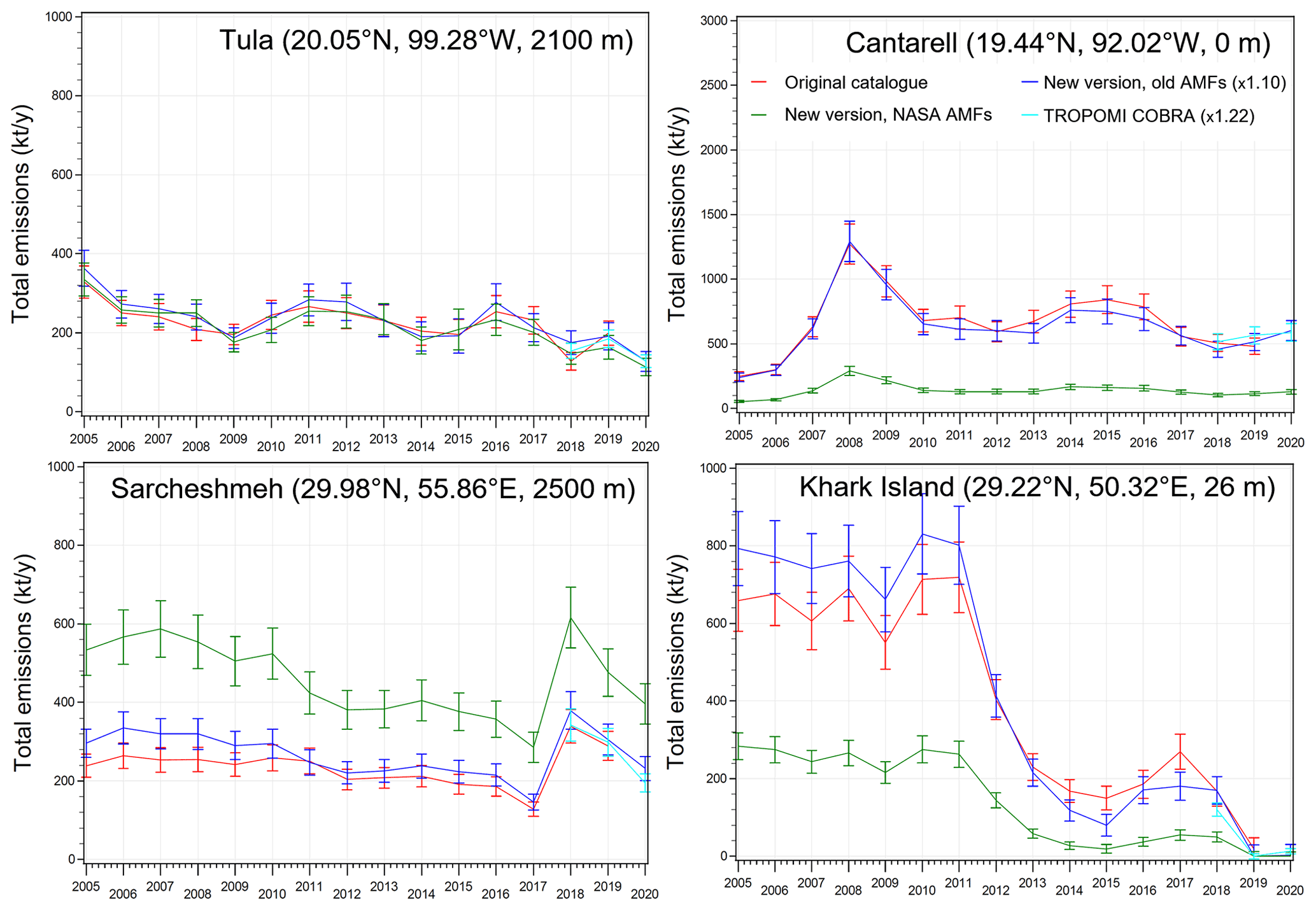
Figure 1Four examples of SO2 emission estimates with 2σ error bars from the original catalogue (red), emissions estimated from OMI version 2 SCD values and converted to VCDs using the same AMFs as in the original catalogue (blue), and emissions estimated using version 2 OMI VCD data (green). We also included TROPOMI-based estimates (cyan). The emission source names, coordinates, and elevations above sea level are shown. TROPOMI-based estimates were increased by 22 % and OMI and OMPS data were increased by 10 % as discussed in the text.
At present, the causes of all the differences between the estimates based on OMI/OMPS version 2 VCDs (i.e. ColumnAmountSO2) and SCDs (i.e. SlantColumnAmountSO2) using the source-specific AMFs is not always clear. In is some cases, it was clear that the difference is related to missing emission information in the underlying CTM (as in the case of Cantarell), although in the others we do not have a good explanation. There are differences in the partial cloud correction calculated between the two SO2 algorithm versions; but analysis of emissions calculated for different cloud fraction thresholds demonstrated that cloud fraction filtering cannot explain the difference. Another factor that could contribute to the difference is the two different versions of the reanalysis wind datasets, but the difference in the wind speed between the two reanalysis versions is on average within 1 %–2 % and is not enough to explain the difference in emissions.
As one of the goals of the catalogue is to improve the existing emissions inventories used in air quality models, we did not use version 2 VCDs that depend on the outputs of such models. Instead, the same approach as in the original catalogue was used, and source-specific AMF values were calculated.
It was found that even if we use the same AMF, emission estimated from OMI version 2 SCDs are on average lower that the values from the original catalogue. Note that the original catalogue was validated against directly measured emissions from the US power plants. To match the original catalogue values, we applied an empirical +10 % correction to OMI and OMPS Version 2 SCD. As a result of this correction, the mean difference in annual emissions between the original catalogue and OMI emission estimates for the version 2 catalogues is less than 1 %.
3.3 New site-specific AMFs
For version 2 of the catalogue, site-specific time-independent AMF values were used to calculate the SO2 VCDs and emissions. A single AMF value is calculated for each source location using a similar approach as in the original catalogue (Fioletov et al., 2016; McLinden et al., 2016). AMFs were first calculated for a subsample of OMI observations (every 100th observation from every third year, within 100 km of the source coordinates). Sampling in this way yields several thousand observations and is sufficient to represent conditions (cloud fraction, viewing and solar geometry, and seasonal sampling) for a given source for all three satellite instruments. The general approach from McLinden et al. (2014) is used, with one main exception. Here, the SO2 profile is estimated based on the elevation of the source and a climatological boundary-layer height (as a function of latitude, longitude, month, and UTC hour) from von Engeln and Teixeira (2013). Between these two altitudes, the profile is assumed to be constant in mixing ratio and zero elsewhere. The single, site-specific AMF is the average over these individual AMFs. In general, there is a relatively small difference between the original and new AMFs. The scatterplot of the AMFs used in the original catalogue vs. the AMFs used in the version 2 catalogue is shown in Fig. 2a. The new AMFs are on average 10 % higher (i.e. emission estimates are lower) for volcanic sources, about 5 % higher for power plants and smelters, and practically unchanged for the oil- and gas-related sources. The ratio of the new to the original AMF values is shown in Fig. 2b as a histogram. On average, the ratio is slightly positive (1.07), it is between 1 and 1.13 for 50 % of all sources and between 0.87 and 1.23 for 90 % of sources. Differences between the old and new version are mainly a result of changes in the OMI effective cloud fraction.

Figure 2(a) Scatterplot of the AMFs used in the original catalogue vs. the AMFs used in the version 2 catalogue. Each dot corresponds to one emission source and the dot colour reflects the source type as shown in the legend. There are total of 555 sources on the plot. The correlation coefficient between the two datasets is 0.98. (b) The distribution of the ratio of the new AMF values to the AMF values in the original catalogue.
3.4 TROPOMI COBRA
The TROPOMI COBRA SO2 algorithm retrieves SCDs (Theys et al., 2021). To ensure consistency, we used the same approach as in the original catalogue: source-specific constant AMFs, although the AMF values were slightly different from the ones used in the original catalogue, as discussed in Sect. 3.3. We also increase the TROPOMI VCDs by 22 %, as mentioned in Sect. 2.2.
3.5 The original vs. new emissions estimates
In summary, there are two main differences between the original and version 2 catalogue OMI-based emission estimates: (1) version 2 is based on a newer version of OMI SO2 data and (2) it uses slightly different AMF values. To illustrate the differences between the two versions, Fig. 3 shows emission estimates from the original catalogue and those from the emission estimates of this study from three satellite instruments grouped by geographical region and source type. The comparison was done for the same 588 sources included in the most recent version of the original catalogue. The original catalogue and the new OMI-based emission estimates show, in general, a good agreement, although the new OMI-based emissions are slightly higher for volcanic sources and lower over India. We observe no substantial regional patterns in the difference between the old and new OMI-based emission estimates. As for annual emissions from individual sources, the difference is within ±10 % in 50 % of cases and within ±23 % in 90 % of cases (only sources emitting >50 kt yr−1, were considered). Figure 3 also shows emission estimates for the version 2 catalogue based on OMPS and TROPOMI COBRA data that are very similar to OMI-based estimates.
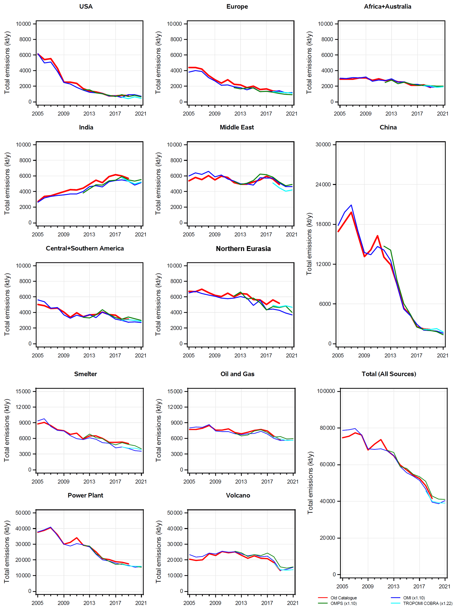
Figure 3Annual SO2 emissions estimated from four satellite datasets: the original catalogue (red), OMI-based estimates for the version 2 catalogue (blue), OMPS-based estimates for the version 2 catalogue (green), and TROPOMI COBRA-based estimates for the version 2 catalogue (cyan). The data are grouped by region (eight top panels), by emission source type (bottom four panels), and the bottom right panel shows total emissions from all sources. TROPOMI-based estimates are adjusted upwards by 22 % to account for the difference in used SO2 cross sections, and OMI and OMPS data are adjusted upwards by 10 % as discussed in the text. Only sources included in the original catalogue with the original AMF values were used in this comparison.
4.1 Merging the emission estimates
The emissions estimates were obtained using data from the three satellite instruments (OMI, OMPS, and TROPOMI). In this section, we discuss some examples of these emission estimates for individual sources. In general, estimates from the different satellite instruments correctly capture long-term changes of emissions. As an illustration, Fig. 4a and b shows the time series of annual emissions from two smelters. The Tsumeb smelter (19.23∘ S, 17.73∘ E), Namibia, was discussed by Ialongo et al. (2018). A sulfur-capture plant was installed there in 2015 to reduce SO2 emissions, and we see that estimates from all three satellite instruments show a twofold decline in emissions thereafter (Fig. 4a) although copper production has increased since 2015 (Ialongo et al., 2018). The overall emissions are relatively low, less than 100 kt yr−1, and OMPS data do not produce a reliable fit, making the emission estimates inaccurate. Another example is the Balqash smelter (46.83∘ N, 74.94∘ E), Kazakhstan, where SO2 emissions also decreased from about 500 kt yr−1 in 2005 (that matches the available information on reported emissions from https://www.thegef.org/sites/default/files/ncsa-documents/2147-22347.pdf, last access: 5 May 2022) to less than 100 kt yr−1 in 2010. A sulfur-capture plant became operational there on 8 June 2008 (http://www.kazakhmys.kz/ru/history, last access: 5 May 2022) and substantially reduced the SO2 emissions in the following years, but then all three satellite data sources show some increase in emissions after 2014.
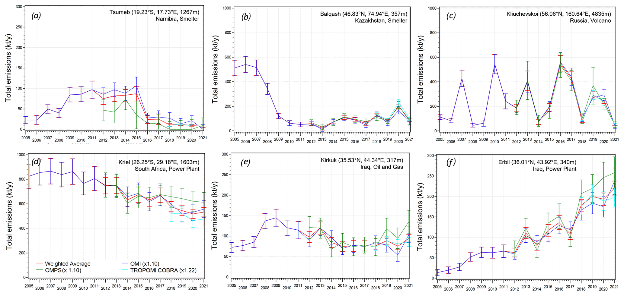
Figure 4Annual emission estimates from the three satellite data sources: OMI (blue), OMPS (green), and TROPOMI (cyan), and their weighted average (red) with 2σ error bars. TROPOMI-based estimates were increased by 22 % and OMI and OMPS data were increased by 10 % as discussed in the text. The emission source names, types, coordinates, and elevations above sea level are shown.
One of the reasons for the difference between OMI, OMPS, and TROPOMI emissions estimates is the size of the source. The three satellite instruments have very different pixel sizes and, therefore, the source plumes observed by them have different widths. For isolated point sources, this should not affect the emission estimates since we use a constant instrument-specific plume width parameter as described in Sect. 3.1. This is illustrated in Fig. 4c, where emissions estimates from a large source (Kluchevskoi volcano (56.06∘ N, 160.64∘ E), Russia) are shown. The source was highly variable in time, but all three instruments reported similar results. However, for sources that consist of multiple point sources with some distance between them, the aggregate plumes can be wider than the plume width used in the fit. Figure 4d shows emissions estimates from a cluster of sources in South Africa, with nine power plants located in an area of over 30 km in diameter. The assigned plume width for TROPOMI and OMI (15 and 20 km respectively) may not be large enough to describe the plume from that cluster of sources. As a result, estimated emissions from TROPOMI and OMI are lower than those from OMPS by 20 % and 10 %, respectively. For non-point sources, the appropriate width parameter is influenced more by the spatial extent of the source and become independent of pixel size. Thus, in the case of the South African cluster, the width parameter would be the same for all three instruments, which would bring them into better relative agreement.
Figure 4e and f show an example of two sources 66 km apart. Erbil gas power station (36.01∘ N, 43.92∘ E) was developed in several stages: the first stage was completed in 2008, the next in 2011–2012, and then in 2014 (https://www.powermag.com/repowering-erbil-power- project-adds-500-mw-to-kurdistan-grid/, last access: 5 May 2022). The SO2 emissions increased from about 20 kt yr−1 in 2005 to about 200 kt yr−1 in 2021. It is possible that this increase in emissions resulted in plumes from Erbil impacting Kirkuk (35.53∘ N, 44.34∘ E), located south-east of Erbil, leading to an increase of estimated emissions for both Kirkuk and Erbil from low-resolution OMPS data in 2019–2021.
OMI and TROPOMI are the main instruments contributing to our emission estimates. The average value of the difference in annual emissions between the TROPOMI COBRA-based estimates and the OMI-based emissions estimates is less than 2 %, the difference is within ±13 % for 50 % of cases and within ±28 % for 90 % of cases (for sources emitting >50 kt yr−1). This is an impressive result given that the instrument characteristics and retrieval algorithms are very different. It should be reminded that the 10 % correction of OMI and OMPS data and 22 % correction of TROPOMI data discussed in Sect. 3 were applied.
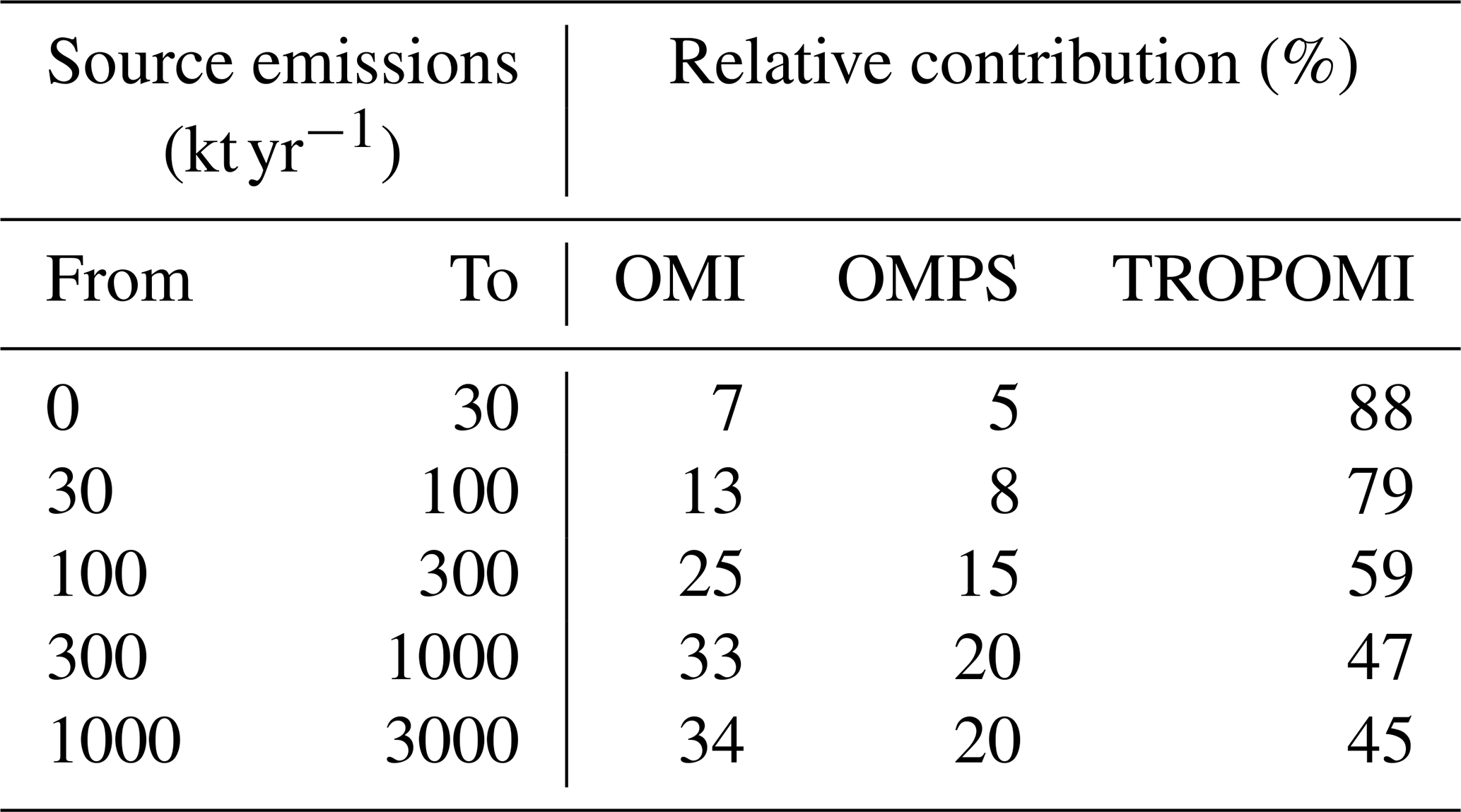
While emission estimates from three satellite instruments are available, it is more convenient for users to have a single emissions dataset. It is also important for future continuation of the catalogue after the end of the Aura/OMI mission (expected before 2025). As such, the final version 2 catalogue emission values were calculated as weighted averages of emission estimates from the three satellite instruments using inverse-variance weighting method; emission estimates for each satellite are weighted in inverse proportion to their variance (i.e. squared fitting uncertainty). The inverse-variance weighted average has the least variance among all weighted averages. The red line in the Fig. 4 shows such weighted averages, i.e. the version 2 catalogue values. For small sources, the variance of TROPOMI-based emission estimates is much lower than that for OMI and OMPS. However, this difference diminishes for larger sources (Fioletov et al., 2020, their Fig. 10). Therefore, the contribution to the weighted average from different satellites depends on the source emission strength. While the actual weights are different from source to source and from year to year, the average weights are given in Table 1. As expected for small sources, the dominant contribution to the weighted average is from TROPOMI (about 90 % for the sources below 30 kt yr−1), while for sources greater 300 kt yr−1, TROPOMI contributes less than 50 %, with 33 % contribution from OMI and 20 % from OMPS.
Table 1Relative contribution of individual satellite instruments to the weighted average for emissions estimate depending on the emission strength for 2018–2021.
Prior to 2012, only OMI data were available, and the weighted average was just OMI-based emissions. In 2012–2017, the weighted average of OMI and OMPS was used. Some sources in some years did not have enough data to produce estimates from OMPS, and in such cases, the average was based on OMI data only. Although statistically significant annual emissions estimates for some sources can be obtained from TROPOMI data only, we nevertheless included OMI and OMPS-based estimates in the weighted average for such sources in the catalogue. Multiyear averages for such sources could be significant even prior to the TROPOMI measurements.
Annual SO2 emissions from the three satellite instruments and their weighted averages grouped by region and source type are shown in Fig. 5. In general, all three satellite instruments agree well. In 2018–2021, the mean difference between OMI and TROPOMI estimates for all regions shown in Fig. 5 is within 10 % except for the northern Eurasia region (Russia, Ukraine, Kazakhstan, and former USSR countries in Central Asia), where it is about 12 %, and the USA. In the case of the USA, the difference is about 40 %. Most of the 57 USA sources were included in the catalogue due to their high emissions in the 2000s. Emissions declined in subsequent years due to scrubber installation, and most of the sources did not produce statistically significant emission estimates in 2018–2021. The OMI-based emission estimates for these sources in 2018–2021 were mostly random noise, and since we reported zero in case of negative emission values in the catalogue, their sum is biased high. If we only consider sources that emitted more than 30 kt yr−1 in 2018–2021, then the difference between TROPOMI and OMI-based estimates is below 10 %. OMPS-based emissions estimates are also slightly higher in some regions for the same reason. As the weights for OMPS are the lowest, their contribution to the weighted average is small. Finally, the difference between the weighted average (i.e. the values from the version 2 catalogue) and mean TROPOMI-based emissions averaged for all eight regions shown in Fig. 5 is between −4 % and +3 %, and for OMI and OMPS it is within ±12 % (for sources >30 kt yr−1).
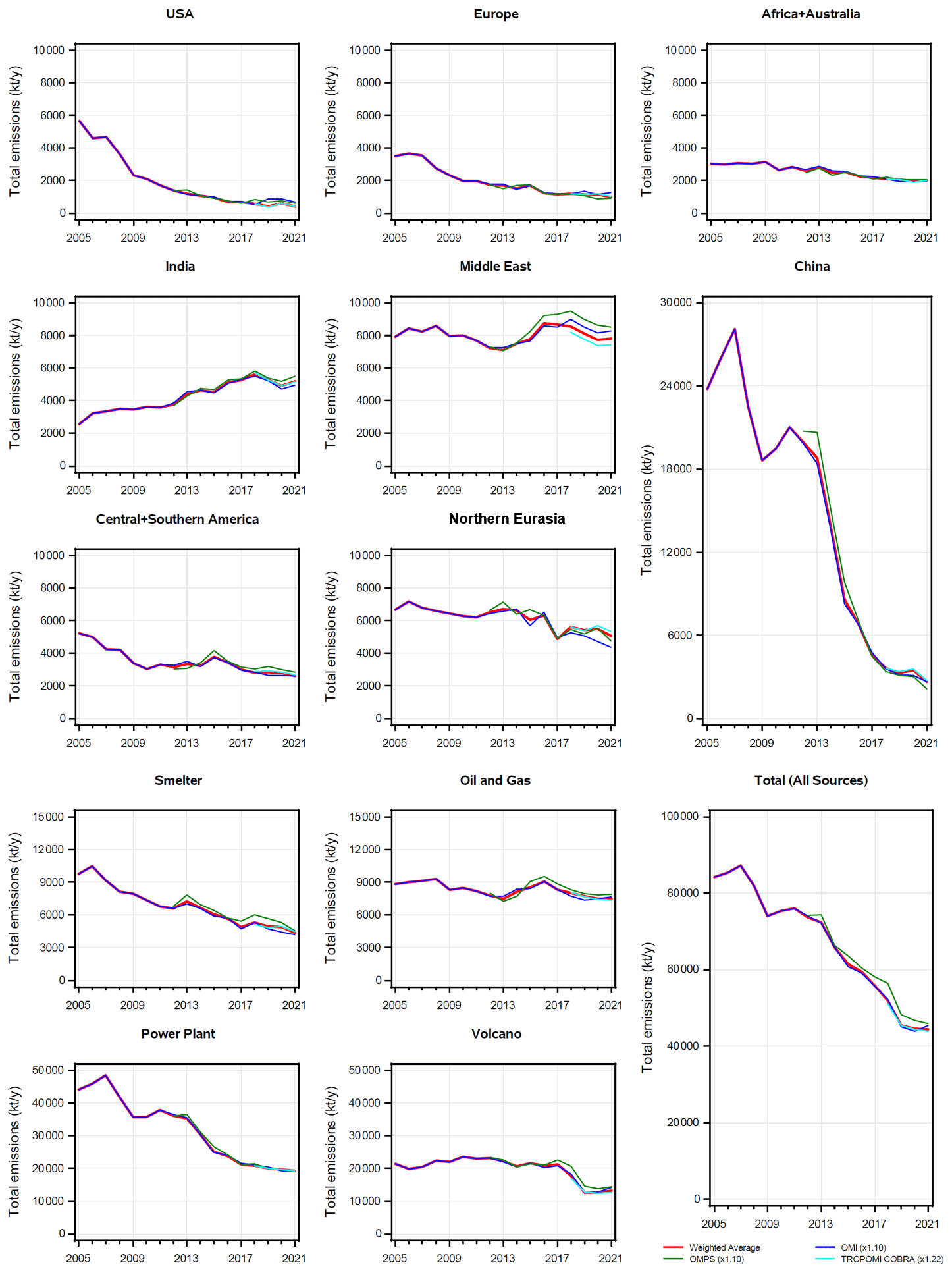
Figure 5Annual SO2 emissions from four satellite datasets: version 2 catalogue OMI VCD data (blue), version 2 catalogue OMPS data (green), version 2 catalogue TROPOMI COBRA data (cyan), and the weighted average (red). The data are grouped by region (eight top panels), by emission source type (bottom four panels), and the bottom right panel shows total emissions from all sources. TROPOMI-based estimates were increased by 22 % and OMI and OMPS data were increased by 10 % as discussed in the text. The weighted average is based on OMI data only in 2005–2011, on OMI and OMPS data in 2012–2017, and on data from all three instruments in 2018–2021.
4.2 New sources and new types of sources
In this section, we discuss some changes in the sources listed in the catalogue and their emissions. The original catalogue contained emission estimates for 491 sources. More sources have been added since then and the 2019 update of the catalogue contained 555 sources. The version 2 catalogue contains 759 sources: 477 power plants, 74 smelters, 102 oil- and gas-related sources, and 106 volcanoes. A map of the sources and the catalogue evolution is shown in Fig. 6. The main reason for adding more sources was a lower emission uncertainty when TROPOMI data are used that made it possible to monitor smaller sources. In addition, better databases of industrial source locations made it possible to identify more sources in past data. Four sources (Severodvinsk, Serov, Turov, and Fushina) were excluded from the original version because their emissions fell below the significance level when version 2 OMI data were used. Some of the sources from the original catalogue did not produce significant emissions during the TROPOMI period (2018–2021): the maximum ratio of estimated annual emissions to their standard deviation was less than 3 for 62 sources and less than 5 for 125 sources.
Figure 6Map of the sources included in the version 2 catalogue. The sources included in the original publication (Fioletov et al., 2016) are shown as black dots, the sources added to the catalogue in 2017–2019 are shown as blue dots, and sources added in the version 2 catalogue are shown as red dots.
There have been numerous changes in emissions from the listed sources since publication of the original catalogue. There is an overall decline in emissions from the US, Europe, and China, as illustrated by Fig. 5. This is largely due to installation of sulfur-capturing devices at power plants in these regions. There is also an overall decline in emissions from smelters. Some smelters, e.g. the Flin-Flon and Thompson smelters (Canada), have been closed, while the others, e.g. Bor (Serbia) and Tsumeb (Namibia), have installed scrubbers that reduced SO2 emissions (Ialongo et al., 2018). While there is a decline in emissions from the oil- and gas-related sources listed in the original catalogue (Fig. 3), there are also a number of new such sources. As a result, overall emissions from this source type remain almost unchanged (Fig. 5).
There are 13 and 43 additional sources in India and China, respectively, mostly coal-burning power plants. Many of them were built earlier, but not included in the original catalogue because it was difficult to properly identify them. The recently released power plant databases made this identification easier. These additional sources increased the estimated total emissions from China and India.
There are 38 additional sources (power plants and oil and gas processing facilities) in the Middle East region. The Al-Khairat power plant (32.43∘ N, 44.28∘ E), Iraq, is one such example. It was built in 2013 and both OMI and TROPOMI-based estimates show a persistent emission of about 170 kt yr−1 in 2014–2021. Another example is a power and desalination plant in Shuqaiq (17.66∘ N, 42.08∘ E), Saudi Arabia (http://sqwec.com/, last access: 16 December 2022), developed in multiple phases. Operations started in 2010 and emissions have increased rapidly since 2016, reaching 300 kt yr−1 in 2021.
In the catalogue, there are three categories of industrial SO2 sources: power plants, smelters, and oil- and gas-sector-related sources. There are, however, some sources that do not fall under any of these categories. One such source is a cluster of small ceramic factories at Morbi (22.8∘ N, 70.9∘ E), India, that was discussed in detail by Kharol et al. (2020). Available emissions inventories do not report any major sources in this region, and yet this source with emissions of about 100 kt yr−1 is one of the largest in the area. Another example is a large cluster of brick kilns near Dhaka (23.63∘ N, 90.45∘ E), Bangladesh. These sources are included in the version 2 catalogue. We decided to list them under the “power plant” category rather than create an additional category.
Cement production is also a source of SO2 emission, where it is produced from coal combustion (Reddy and Venkataraman, 2002). Emissions from cement plants are too small, less than 50 kt yr−1, to be detected by OMI, but two such sources (Shree (26.3∘ N, 74.13∘ E), India and Thap Kwang (14.63∘ N, 101.08∘ E), Thailand), can be detected by TROPOMI and are included in version 2 catalogue. Each of these sources is a cluster of several individual cement factories. We did not introduce a new source type in the catalogue and assigned the “power plant” source type for these sources (but included this information in the comment column).
It is rare that new large emissions sources appear at high latitudes. Two examples are production plants in the Russian Arctic near town of Usinsk: Bajandyskaya (66.432∘ N, 56.6∘ E) and East Lambeishor (66.764∘ N, 56.192∘ E) (https://energybase.ru/compressor-station/oil-treatment-plant-opf-east-lambeishor, last access: 26 January 2022) that began their operation in about 2014. The plants are 42 km apart and they process the fluid mixture of oil, gas, and water from oil wells, remove hydrogen sulfide, and prepare the oil for further use. We assume that the main SO2 emission sources are the gas flares that are clearly visible on satellite images displayed in Google Maps. The TROPOMI-based emissions are about 110 kt yr−1 for Bajandyskaya and about 70 kt yr−1 for Lambeishor, although there could be some double-counting of emission due to their close proximity. OMI data are too noisy for reliable emission estimates from these two sources.
Emissions sources can often be detected from multiyear mean SO2 VCD maps and then confirmed using high-resolution satellite imagery (Dammers et al., 2019; Fioletov et al., 2016; McLinden et al., 2016). Satellite images helped us to link some SO2 hotspots with powerships, i.e. power plants installed on a moving platform, like a ship. One such source was identified at the port of Dakar (14.69∘ N, 17.43∘ W), Senegal, and is included in the new catalogue. Karpowership's powership with 235 MW capacity was deployed there in October 2019 (https://karpowership.com/en/project-senegal, last access: 26 January 2022). The estimated emissions are about 40 kt yr−1, but it is likely the combined emissions from the powership and the existing power plant in the area. Another example is Port de Mariel (23.02∘ N, 82.75∘ W), Cuba, where three powerships with a total capacity of 184 MW were installed in November 2019 (https://karpowership.com/en/project-cuba, last access: 26 January 2022) in addition to the existing power plant. As a result, total emission from Mariel increased from about 70 kt yr−1 to about 90 kt yr−1. The contribution of such powerships to the total national electricity needs in both these cases are rather substantial, about 10 %. Large powerships have also been in operation at Zouk (33.96∘ N, 35.61∘ E) and Jieh (33.65∘ N, 35.4∘ E), Lebanon, since 2013, each with a capacity of 202 MW (https://karpowership.com/en/lebanon, last access: 26 January 2022). The powership at Jieh is included in the new catalogue and its emissions are estimated to be about 20–30 kt yr−1. In the case of Zouk, the powership was located near a power plant that has already been included in the original catalogue.
Version 2 catalogue emission estimates for OMI and, particularly, TROPOMI COBRA show a lower noise level in the South Atlantic Anomaly area. This made it possible to estimate emissions from two volcanic sources (Planchón-Peteroa (35.27∘ S, 70.57∘ W), Argentina and Lascar (23.37∘ S, 67.68∘ W), Chile) and from four oil- and gas-related sources in Brazil.
Six new volcanic sources were added to the catalogue. In addition to the two mentioned above, there are three others located in Alaska (Makushin), the Kuril Islands (Ebeko), and Nicaragua (Momotombo). Their maximum annual emissions range from 50 to 150 kt yr−1. We also added La Palma volcano, Canary Islands (https://volcano.si.edu/volcano.cfm?vn=383010, last access: 26 May 2022) that became active in 2021, although most of SO2 detected there was emitted during a major eruption in September–December 2021, and therefore not reflected in the catalogue due to the screening of high transient volcanic SO2 VCDs.
4.3 Emissions by region and source type
Figure 7 illustrates the emission sources listed in the catalogue at the beginning (2005) and the end (2021) of the available data period. The symbol size is proportional to the emission strength, while the colour represents the source type. Industrial sources with annual emissions under 3 standard errors (σ) of the estimate are not shown. There is a clear decline in the number of detectable sources over the US, China, and Europe, despite 3 times lower emission estimates uncertainties for small sources due to TROPOMI data in recent years. For example, only 11 industrial sources produced emissions above 3σ level in the US in 2021, while there were 57 such sources in 2005. There are several clusters of sources visible on the Fig. 7 maps: power plants in India and China, oil- and gas-related sources in the Middle East, and a number of smelters along the west coast of South America. The largest sources such as Norilsk and the cluster of power plants in South Africa demonstrated little changes in their emissions. Figure 7 also shows an increase in the number of sources in India and the Middle East.
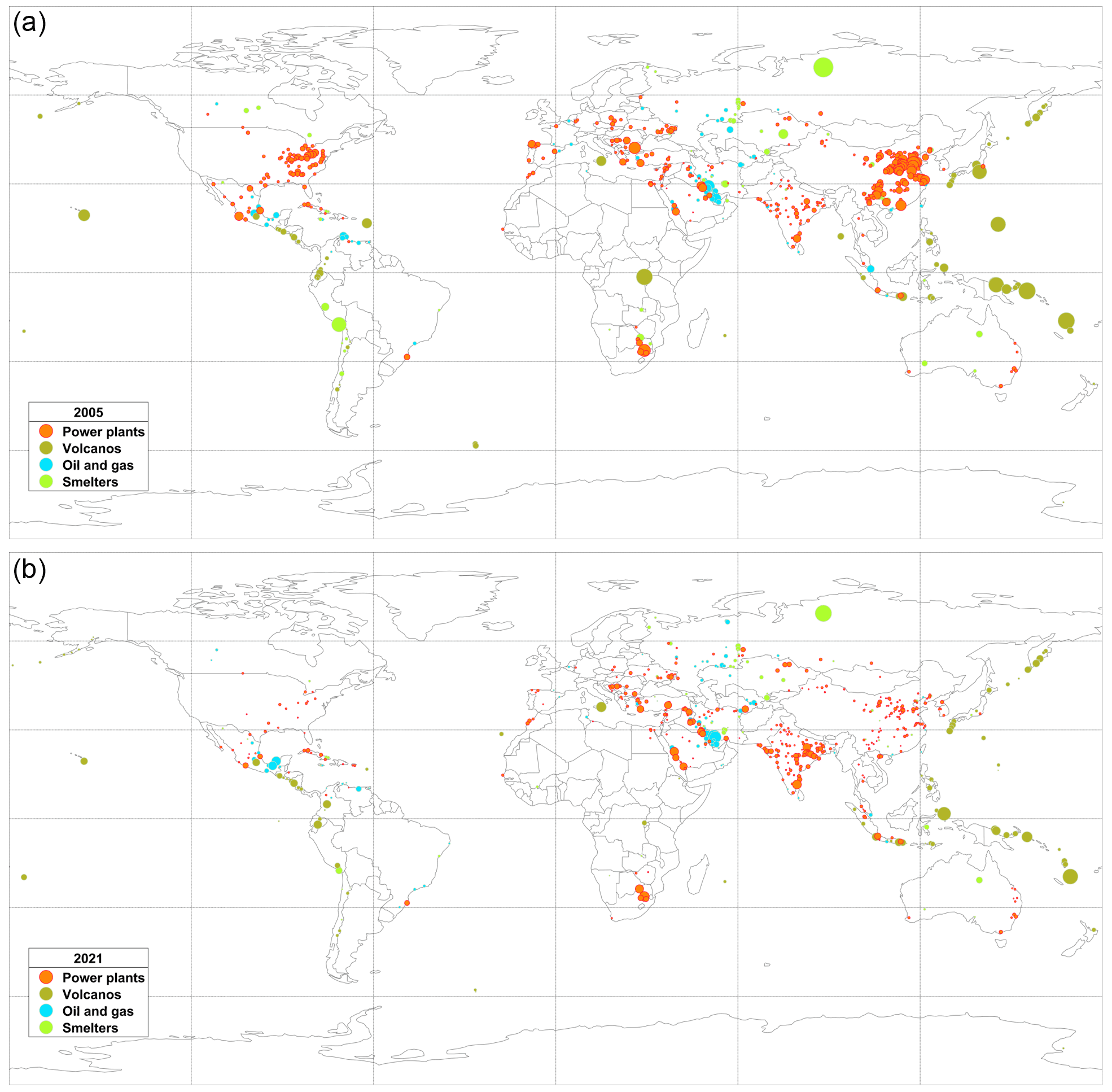
Figure 7SO2 emissions sources listed in the version 2 catalogue for 2005 (a) and 2021 (b). Only sources where the ratio of the emission value to its standard deviation is greater than 3 are shown. The size of the symbols is proportional to the annual emission values.
While the absolute values of emissions are shown in Fig. 7, the relative contribution to total emissions in different years grouped by the source type as well as country and/or region is shown in Fig. 8. The decline in emissions from China, the US, and Europe was largely related to the power generation sector. As a result, total SO2 emissions from power plants declined by about 60 %, and their relative contribution to total SO2 emissions has declined since 2005 from 52 % to 44 %. Emissions from smelters demonstrated a similar decline and the relative contribution of smelters remains unchanged (10 %–12 %). However, emissions from oil- and gas-related sources do not show any changes, and the fraction of emissions related to the oil and gas industry has increased from 11 % to 17 %.
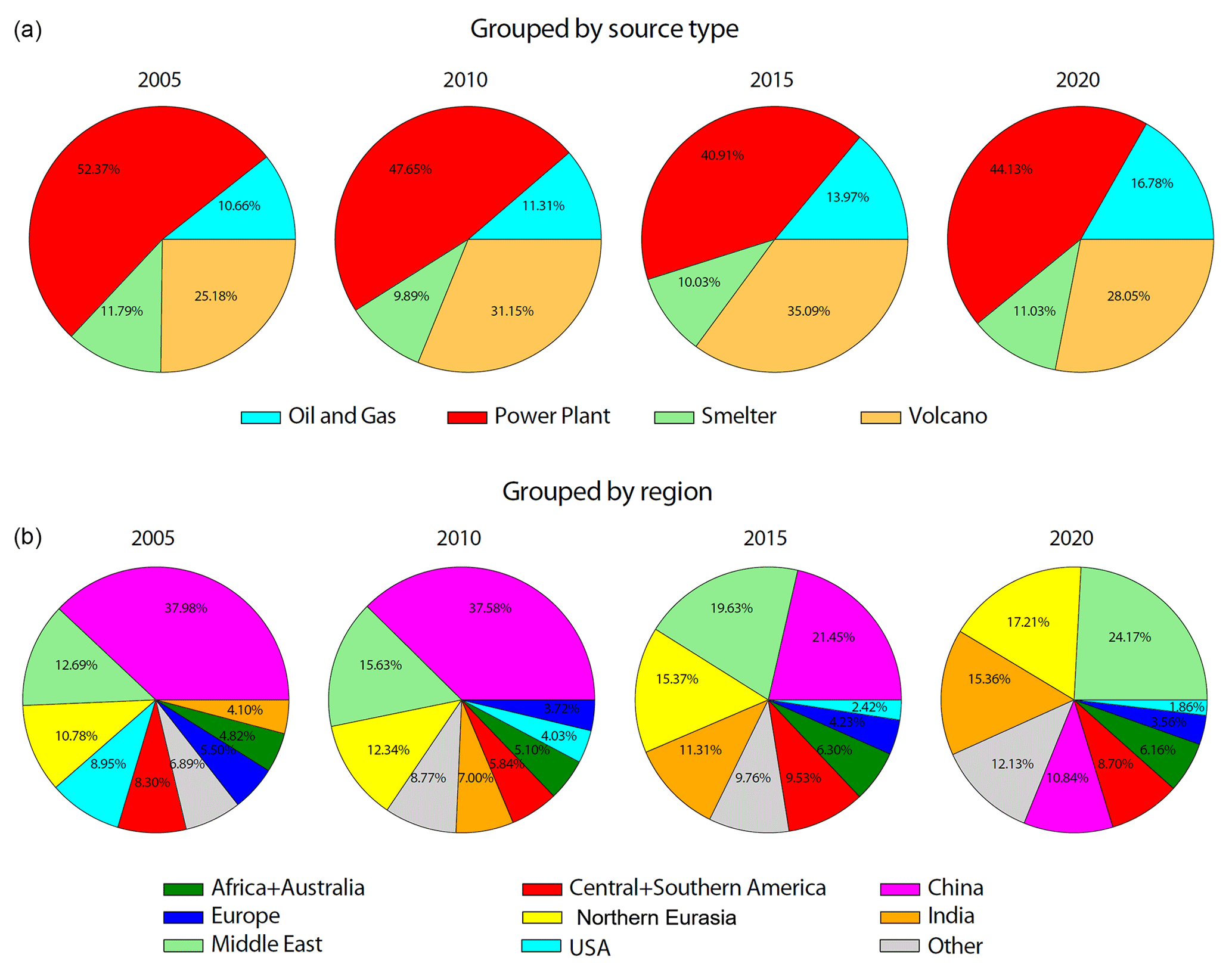
Figure 8(a) Pie charts of contributions to total SO2 emissions by the source type. Power plants are the main source of emissions and degassing volcanoes contribute between one-quarter to one-third of total emissions. (b) Pie charts of contributions to total anthropogenic SO2 emissions by region.
On a global scale, the new catalogue data show an approximate 50 % decline in global SO2 emissions between 2005 and 2021, although the SO2 emissions appear to have levelled off before 2008, between 2009 and 2013, and in the last 3 years. On a regional level, there has been a remarkable decline in emissions from the US and Europe since 2005. Their emissions also levelled off in the last 3–4 years. The relative contributions of the US and European emissions to the total anthropogenic emissions are about 2 % and 3.5 %, respectively. Emissions from China increased at the beginning of the record, but they declined thereafter. China contributed nearly 40 % to total anthropogenic emissions in 2005–2010, and its contribution declined to under 11 % in 2020. Emissions from India have surpassed emissions from China after 2015 (Li et al., 2017), but they levelled off in recent years. At present, they account for 15 % of the total anthropogenic emissions. Emissions from the Middle East show some increase, although they also levelled off in the recent years. Nevertheless, their relative contribution increased from 13 % in 2005 to 24 % in 2020. The northern Eurasia region also demonstrated some decline in emissions, but its relative contribution increased from 11 % in 2005 to 17 % in 2020.
Degassing volcanoes contribute between one-quarter and one-third of total SO2 emissions. After remaining roughly constant for the first 15 years or so, total volcanic emissions started declining in 2018 and were lower by up to 40 % in 2019–2021. This was mainly due to a very large decline (1000–2000 kt yr−1) in emissions from some strong volcanic sources, including Kilauea (Hawaii) as well as the Aoba and Ambrym (Vanuatu) volcanoes.
The full version 2 SO2 point source catalogue is available from the NASA global sulfur dioxide monitoring home page (https://so2.gsfc.nasa.gov/measures.html, last access: 11 November 2022). The direct link to the dataset is https://so2.gsfc.nasa.gov/kml/Catalogue_SO2_2022.xls (last access: 16 December 2022). The DOI identifier is https://disc.gsfc.nasa.gov/datasets/MSAQSO2L4_1/summary (last access: 16 December 2022) (https://doi.org/10.5067/MEASURES/SO2/DATA406; Fioletov et al., 2022).
The TROPOMI COBRA SO2 dataset is available from co-author Nicolas Theys on request. The OMI and OMPS PCA SO2 data are publicly available from the Goddard Earth Sciences (GES) Data and Information Services Center (DISC) (https://doi.org/10.5067/Aura/OMI/DATA2022, Li et al., 2020a, and https://doi.org/10.5067/MEASURES/SO2/DATA205, Li et al., 2020b).
To update the original catalogue of large SO2 sources and emissions (Fioletov et al., 2016), a new version 2 of the catalogue was developed that merges the data from three satellite instruments, OMI, OMPS, and TROPOMI, for the 2005–2021 period. For OMI and OMPS, version 2 SO2 data (Li et al., 2020c) were used. For TROPOMI, the COBRA research data product (Theys et al., 2021) was used. For all datasets, SCDs were converted to VCDs using a set of site-specific AMFs as in the original catalogue, although for catalogue version 2, the AMFs were recalculated using the most recent data on albedo and climatological aerosol data. As in the original catalogue, only measurements under snow- and ice-free as well as mostly cloud-free conditions were used in the analysis. The total number of sources in the version 2 catalogue is 759, including 477 power plants, 74 smelters, 102 oil- and gas-related sources, and 106 volcanoes. However, some of these sources were not active in recent years: 62 sources from the original catalogue do not produce detectable emissions in 2018–2021. Four sources were excluded from the original catalogue because their estimated emissions using version 2 OMI data are below the significance level. It should be mentioned that simple attribution of sources is not always possible because at some sites multiple different industrial sources are clustered in close proximity.
The SO2 emission estimation algorithm is identical to that used in the original study (Fioletov et al., 2016), to assure the continuity of the old and new emissions estimates. Unlike the original catalogue, where ERA-Interim reanalysis wind data were used, the new catalogue employed ERA5 reanalysis data. For consistency with the original catalogue, the values obtained from version 2 OMI and OMPS-based estimates were increased by +10 %. For TROPOMI, a +22 % correction was applied to account for differences in temperatures for the SO2 absorption coefficients used in the retrievals. Note that the original catalogue also had empirical corrections applied to ensure agreement with reliable at stack emission measurements in the US and other countries (Fioletov et al., 2016).
The version 2 catalogue emissions are weighted averages of OMI, OMPS, and TROPOMI-based emission estimates using an inverse-variance weighting method. If emission estimates from all three satellite instruments are available, the TROPOMI-based estimates dominate in the weighted average for small sources (about 90 % contribution for sources under 30 kt yr−1). For large sources (300 kt yr−1), contributions from TROPOMI, OMI, and OMPS-based emission estimates were 47 %, 33 %, and 20 %, respectively.
As previously discussed (Fioletov et al., 2016; Theys et al., 2021), the emission detection limit is typically about 30–40 kt yr−1 for OMI data and 8 kt yr−1 for TROPOMI data, although these values vary from source to source depending on the AMF values and local conditions.
Systematic differences between the emission estimates from OMI, OMPS, and TROPOMI data are less than 12 % for all eight large regions analysed in this study. However, the difference could be larger for individual sources. The differences in annual emissions between the TROPOMI COBRA-based estimates and the OMI-based estimates are within ±13 % for 50 % of cases and within ±28 % for 90 % of cases (only sources emitting >50 kt yr−1 were considered). Large differences are typically seen for sources comprised of several individual point sources. Sources in close proximity are one of the main obstacles to reliable emission estimations when using the point-source emission algorithm. Emissions from sources 60–80 km apart typically can be reliably estimated, while sources under 20–30 km apart are counted as a single source. However, it also depends on the wind climatology and emissions strength of the sources. For user convenience, for each catalogue entry, we included information about the nearest other catalogue source and the distance to that source.
The original catalogue was successfully used to improve emission inventories used in air quality and climate models, as well as to monitor emission reductions due to sulfur-capturing device installation and other applications. The version 2 catalogue updates the emission estimates using the most recent version of OMI SO2 data and utilises emission estimates from two other operational UV satellite instruments, OMPS and TROPOMI. For user convenience, the version 2 catalogue dataset also contains emission estimates for individual satellite instruments that can be further used for analysis and cross-validation of the different satellite data sources.
VEF prepared the paper and figures with contributions from all the co-authors. VEF and CAM developed the emission estimation algorithm. VEF, CAM and DG processed satellite data and estimated the emissions. CL, NK, and JJ developed the OMI and OMPS PCA version 2 algorithms and provided data. NT developed the TROPOMI COBRA algorithms and provided data. IA developed some of the emission data visualisation tools. PJTL provided support for hosting the catalogue. SC contributed to cataloguing of volcanic sources and interpreted the estimated volcanic emissions.
The contact author has declared that none of the authors has any competing interests.
Publisher's note: Copernicus Publications remains neutral with regard to jurisdictional claims in published maps and institutional affiliations.
We thank Keith Evans and Garrett Layne for developing SO2 emissions website: https://so2.gsfc.nasa.gov/measures.html (last access: 16 December 2022). We also thank EU/ESA/KNMI/DLR for providing the TROPOMI/S5P Level 1 products. Can Li, Nickolay Krotkov, and Joanna Joiner acknowledge support from the NASA Earth Science Division Aura Science Team, Suomi NPP Science Team, and US participating investigator programmes. OMI PCA SO2 data used in this study have been publicly released as part of the Aura OMI Sulfur Dioxide Data Product – OMSO2 – and can be obtained free of charge from the Goddard Earth Sciences (GES) Data and Information Services Center (DISC, http://daac.gsfc.nasa.gov/, last access: 16 December 2022). Nicolas Theys acknowledges support from ESA (S5P-PAL and S5P MPC projects) and BELSO Prodex-Trace S5P.
This paper was edited by Bo Zheng and reviewed by two anonymous referees.
Beirle, S., Hörmann, C., Penning de Vries, M., Dörner, S., Kern, C., and Wagner, T.: Estimating the volcanic emission rate and atmospheric lifetime of SO2 from space: a case study for Kīlauea volcano, Hawai`i, Atmos. Chem. Phys., 14, 8309–8322, https://doi.org/10.5194/acp-14-8309-2014, 2014.
Beirle, S., Borger, C., Dörner, S., Eskes, H., Kumar, V., de Laat, A., and Wagner, T.: Catalog of NOx emissions from point sources as derived from the divergence of the NO2 flux for TROPOMI, Earth Syst. Sci. Data, 13, 2995–3012, https://doi.org/10.5194/essd-13-2995-2021, 2021.
Bovensmann, H., Burrows, J. P., Buchwitz, M., Frerick, J., Noël, S., Rozanov, V. V., Chance, K. V., and Goede, A. P. H.: SCIAMACHY: Mission objectives and measurement modes, J. Atmos. Sci., 56, 127–150, 1999.
Callies, J., Corpaccioli, E., Eisinger, M., Hahne, A., and Lefebvre, A.: GOME-2-Metop's second-generation sensor for operational ozone monitoring, ESA Bulletin-European Space Agency, 102 28–36, https://esamultimedia.esa.int/multimedia/publications/ESA-Bulletin-102/offline/download.pdf (last access: 16 December 2022), 2000.
Carn, S. A., Fioletov, V. E., McLinden, C. A., Li, C., and Krotkov, N. A.: A decade of global volcanic SO2 emissions measured from space, Sci. Rep.-UK, 7, 44095, https://doi.org/10.1038/srep44095, 2017.
Copernicus Climate Change Service (C3S): ERA5: Fifth generation of ECMWF atmospheric reanalyses of the global climate, Copernicus Climate Change Service Climate Data Store (CDS), https://cds.climate.copernicus.eu/cdsapp{#}!/home (last access: 20 June 2020), 2017.
Dammers, E., McLinden, C. A., Griffin, D., Shephard, M. W., Van Der Graaf, S., Lutsch, E., Schaap, M., Gainairu-Matz, Y., Fioletov, V., Van Damme, M., Whitburn, S., Clarisse, L., Cady-Pereira, K., Clerbaux, C., Coheur, P. F., and Erisman, J. W.: NH3 emissions from large point sources derived from CrIS and IASI satellite observations, Atmos. Chem. Phys., 19, 12261–12293, https://doi.org/10.5194/acp-19-12261-2019, 2019.
de Foy, B., Krotkov, N. A., Bei, N., Herndon, S. C., Huey, L. G., Martínez, A.-P., Ruiz-Suárez, L. G., Wood, E. C., Zavala, M., and Molina, L. T.: Hit from both sides: tracking industrial and volcanic plumes in Mexico City with surface measurements and OMI SO2 retrievals during the MILAGRO field campaign, Atmos. Chem. Phys., 9, 9599–9617, https://doi.org/10.5194/acp-9-9599-2009, 2009.
de Foy, B., Lu, Z., Streets, D. G., Lamsal, L. N., and Duncan, B. N.: Estimates of power plant NOx emissions and lifetimes from OMI NO2 satellite retrievals, Atmos. Environ., 116, 1–11, https://doi.org/10.1016/j.atmosenv.2015.05.056, 2015.
de Graaf, M., Sihler, H., Tilstra, L. G., and Stammes, P.: How big is an OMI pixel?, Atmos. Meas. Tech., 9, 3607–3618, https://doi.org/10.5194/amt-9-3607-2016, 2016.
Dee, D. P., Uppala, S. M., Simmons, A. J., Berrisford, P., Poli, P., Kobayashi, S., Andrae, U., Balmaseda, M. A., Balsamo, G., Bauer, P., Bechtold, P., Beljaars, A. C. M., van de Berg, L., Bidlot, J., Bormann, N., Delsol, C., Dragani, R., Fuentes, M., Geer, A. J., Haimberger, L., Healy, S. B., Hersbach, H., Hólm, E. V., Isaksen, L., Kållberg, P., Köhler, M., Matricardi, M., McNally, A. P., Monge-Sanz, B. M., Morcrette, J.-J., Park, B.-K., Peubey, C., de Rosnay, P., Tavolato, C., Thépaut, J.-N., and Vitart, F.: The ERA-Interim reanalysis: Configuration and performance of the data assimilation system, Q. J. Roy. Meteor. Soc., 137, 553–597, https://doi.org/10.1002/qj.828, 2011.
Dentener, F., Drevet, J., Lamarque, J. F., Bey, I., Eickhout, B., Fiore, A. M., Hauglustaine, D., Horowitz, L. W., Krol, M., Kulshrestha, U. C., Lawrence, M., Galy-Lacaux, C., Rast, S., Shindell, D., Stevenson, D., Van Noije, T., Atherton, C., Bell, N., Bergman, D., Butler, T., Cofala, J., Collins, B., Doherty, R., Ellingsen, K., Galloway, J., Gauss, M., Montanaro, V., Müller, J. F., Pitari, G., Rodriguez, J., Sanderson, M., Solmon, F., Strahan, S., Schultz, M., Sudo, K., Szopa, S., and Wild, O.: Nitrogen and sulfur deposition on regional and global scales: A multimodel evaluation, Global Biogeochem. Cy., 20, GB4003, https://doi.org/10.1029/2005GB002672, 2006.
Eisinger, M. and Burrows, J. P.: Tropospheric sulfur dioxide observed by the ERS-2 GOME instrument, Geophys. Res. Lett., 25, 4177–4180, 1998.
Fioletov, V., McLinden, C. A., Kharol, S. K., Krotkov, N. A., Li, C., Joiner, J., Moran, M. D., Vet, R., Visschedijk, A. J. H., and Denier van der Gon, H. A. C.: Multi-source SO2 emission retrievals and consistency of satellite and surface measurements with reported emissions, Atmos. Chem. Phys., 17, 12597–12616, https://doi.org/10.5194/acp-17-12597-2017, 2017.
Fioletov, V., McLinden, C. A., Griffin, D., Theys, N., Loyola, D. G., Hedelt, P., Krotkov, N. A., and Li, C.: Anthropogenic and volcanic point source SO2 emissions derived from TROPOMI on board Sentinel-5 Precursor: first results, Atmos. Chem. Phys., 20, 5591–5607, https://doi.org/10.5194/acp-20-5591-2020, 2020.
Fioletov, V., McLinden, C. A., Griffin, D., Abboud, I., Krotkov, N., Leonard, P. J. T., Li, C., Joiner, J., Theys, N., and Carn, S.: Multi-Satellite Air Quality Sulfur Dioxide (SO2) Sources and Emissions Database Long-Term L4 Global V2, edited by: Leonard, P., Goddard Earth Science Data and Information Services Center (GES DISC) [data set], Greenbelt, MD, USA, https://doi.org/10.5067/MEASURES/SO2/DATA406, 2022.
Fioletov, V. E., McLinden, C. A., Krotkov, N., Yang, K., Loyola, D. G., Valks, P., Theys, N., Van Roozendael, M., Nowlan, C. R., Chance, K., Liu, X., Lee, C., and Martin, R. V.: Application of OMI, SCIAMACHY, and GOME-2 satellite SO2 retrievals for detection of large emission sources, J. Geophys. Res.-Atmos., 118, 11399–11418, https://doi.org/10.1002/jgrd.50826, 2013.
Fioletov, V. E., McLinden, C. A., Krotkov, N., and Li, C.: Lifetimes and emissions of SO2 from point sources estimated from OMI, Geophys. Res. Lett., 42, 1969–1976, https://doi.org/10.1002/2015GL063148, 2015.
Fioletov, V. E., McLinden, C. A., Krotkov, N., Li, C., Joiner, J., Theys, N., Carn, S., and Moran, M. D.: A global catalogue of large SO2 sources and emissions derived from the Ozone Monitoring Instrument, Atmos. Chem. Phys., 16, 11497–11519, https://doi.org/10.5194/acp-16-11497-2016, 2016.
Fischer, T. P., Arellano, S., Carn, S., Aiuppa, A., Galle, B., Allard, P., Lopez, T., Shinohara, H., Kelly, P., Werner, C., Cardellini, C., and Chiodini, G.: The emissions of CO2 and other volatiles from the world's subaerial volcanoes, Sci. Rep.-UK, 9, 1–11, https://doi.org/10.1038/s41598-019-54682-1, 2019.
Flynn, L., Long, C., Wu, X., Evans, R., Beck, C. T., Petropavlovskikh, I., Mcconville, G., Yu, W., Zhang, Z., Niu, J., Beach, E., Hao, Y., Pan, C., Sen, B., Novicki, M., Zhou, S., and Seftor, C.: Performance of the Ozone Mapping and Profiler Suite (OMPS) products, J. Geophys. Res.-Atmos., 119, 6181–6195, https://doi.org/10.1002/2013JD020467, 2014.
Hansell, A. and Oppenheimer, C.: Health Hazards from Volcanic Gases: A Systematic Literature Review, Archives of Environmental Health: An International Journal, 59, 628–639, https://doi.org/10.1080/00039890409602947, 2010.
Helfrich, S. R., McNamara, D., Ramsay, B. H., Baldwin, T., and Kasheta, T.: Enhancements to, and forthcoming developments in the Interactive Multisensor Snow and Ice Mapping System (IMS), Hydrol. Process., 21, 1576–1586, https://doi.org/10.1002/hyp.6720, 2007.
Hutchinson, T. C. and Whitby, L. M.: The effects of acid rainfall and heavy metal particulates on a boreal Forest ecosystem near the sudbury smelting region of Canada, Water Air Soil Poll., 7, 421–438, https://doi.org/10.1007/BF00285542, 1977.
Ialongo, I., Fioletov, V., McLinden, C., Jåfs, M., Krotkov, N., Li, C., and Tamminen, J.: Application of satellite-based sulfur dioxide observations to support the cleantech sector: Detecting emission reduction from copper smelters, Environ. Technol. Innov., 12, 172–179, https://doi.org/10.1016/j.eti.2018.08.006, 2018.
Kharol, S. K., Fioletov, V., McLinden, C. A., Shephard, M. W., Sioris, C. E., Li, C., and Krotkov, N. A.: Ceramic industry at Morbi as a large source of SO2 emissions in India, Atmos. Environ., 223, 117243, https://doi.org/10.1016/j.atmosenv.2019.117243, 2020.
Khokhar, M. F., Platt, U., and Wagner, T.: Temporal trends of anthropogenic SO2 emitted by non-ferrous metal smelters in Peru and Russia estimated from Satellite observations, Atmos. Chem. Phys. Discuss., 8, 17393–17422, https://doi.org/10.5194/acpd-8-17393-2008, 2008.
Klimont, Z., Smith, S. J., and Cofala, J.: The last decade of global anthropogenic sulfur dioxide: 2000–2011 emissions, Environ. Res. Lett., 8, 014003, https://doi.org/10.1088/1748-9326/8/1/014003, 2013.
Krotkov, N. A., Carn, S. A., Krueger, A. J., Bhartia, P. K., and Yang, K.: Band Residual Difference Algorithm for Retrieval of SO2 From the Aura Ozone Monitoring Instrument (OMI), IEEE T. Geosci. Remote, 44, 1259–1266, 2006.
Krotkov, N. A., McClure, B., Dickerson, R. R., Carn, S. A., Li, C., Bhartia, P. K., Yang, K., Krueger, A. J., Li, Z., Levelt, P. F., Chen, H., Wang, P., and Lu, D.: Validation of SO2 retrievals from the Ozone Monitoring Instrument over NE China, J. Geophys. Res., 113, D16S40, https://doi.org/10.1029/2007JD008818, 2008.
Krotkov, N. A., McLinden, C. A., Li, C., Lamsal, L. N., Celarier, E. A., Marchenko, S. V., Swartz, W. H., Bucsela, E. J., Joiner, J., Duncan, B. N., Boersma, K. F., Veefkind, J. P., Levelt, P. F., Fioletov, V. E., Dickerson, R. R., He, H., Lu, Z., and Streets, D. G.: Aura OMI observations of regional SO2 and NO2 pollution changes from 2005 to 2015, Atmos. Chem. Phys., 16, 4605–4629, https://doi.org/10.5194/acp-16-4605-2016, 2016.
Krueger, A. J.: Sighting of El Chichón sulfur dioxide clouds with the Nimbus 7 Total Ozone Mapping Spectrometer, Science, 220, 1377–1378, 1983.
Levelt, P. F., van den Oord, G. H. J., Dobber, M. R., Malkki, A., Stammes, P., Lundell, J. O. V., and Saari, H.: The Ozone Monitoring Instrument, IEEE T. Geosci. Remote, 44, 1093–1101, https://doi.org/10.1109/TGRS.2006.872333, 2006.
Levelt, P. F., Joiner, J., Tamminen, J., Veefkind, J. P., Bhartia, P. K., Stein Zweers, D. C., Duncan, B. N., Streets, D. G., Eskes, H., van der A, R., McLinden, C., Fioletov, V., Carn, S., de Laat, J., DeLand, M., Marchenko, S., McPeters, R., Ziemke, J., Fu, D., Liu, X., Pickering, K., Apituley, A., González Abad, G., Arola, A., Boersma, F., Chan Miller, C., Chance, K., de Graaf, M., Hakkarainen, J., Hassinen, S., Ialongo, I., Kleipool, Q., Krotkov, N., Li, C., Lamsal, L., Newman, P., Nowlan, C., Suleiman, R., Tilstra, L. G., Torres, O., Wang, H., and Wargan, K.: The Ozone Monitoring Instrument: overview of 14 years in space, Atmos. Chem. Phys., 18, 5699–5745, https://doi.org/10.5194/acp-18-5699-2018, 2018.
Li, C., Joiner, J., Krotkov, N. A., and Bhartia, P. K.: A fast and sensitive new satellite SO2 retrieval algorithm based on principal component analysis: Application to the ozone monitoring instrument, Geophys. Res. Lett., 40, 6314–6318, https://doi.org/10.1002/2013GL058134, 2013.
Li, C., McLinden, C., Fioletov, V., Krotkov, N., Carn, S., Joiner, J., Streets, D., He, H., Ren, X., Li, Z., and Dickerson, R. R.: India Is Overtaking China as the World's Largest Emitter of Anthropogenic Sulfur Dioxide, Sci. Rep.-UK, 7, 14304, https://doi.org/10.1038/s41598-017-14639-8, 2017.
Li, C., Krotkov, N. A., Leonard, P. J. T., and Joiner, J.: OMI/Aura Sulphur Dioxide (SO2) Total Column 1-orbit L2 Swath 13×24 km V003, Goddard Earth Sci. Data Inf. Serv. Cent. (GES DISC) [data set], Greenbelt, MD, USA, https://doi.org/10.5067/Aura/OMI/DATA2022, 2020a.
Li, C., Krotkov, N. A., Leonard, P. J. T., and Joiner, J.: OMPS/NPP PCA SO2 Total Column 1-Orbit L2 Swath 50×50 km V2, Goddard Earth Sci. Data Inf. Serv. Cent. (GES DISC) [data set], Greenbelt, MD, USA, https://doi.org/10.5067/MEASURES/SO2/DATA205, 2020b.
Li, C., Krotkov, N. A., Leonard, P. J. T., Carn, S., Joiner, J., Spurr, R. J. D., and Vasilkov, A.: Version 2 Ozone Monitoring Instrument SO2 product (OMSO2 V2): new anthropogenic SO2 vertical column density dataset, Atmos. Meas. Tech., 13, 6175–6191, https://doi.org/10.5194/amt-13-6175-2020, 2020c.
Liu, F., Choi, S., Li, C., Fioletov, V. E., McLinden, C. A., Joiner, J., Krotkov, N. A., Bian, H., Janssens-Maenhout, G., Darmenov, A. S., and da Silva, A. M.: A new global anthropogenic SO2 emission inventory for the last decade: a mosaic of satellite-derived and bottom-up emissions, Atmos. Chem. Phys., 18, 16571–16586, https://doi.org/10.5194/acp-18-16571-2018, 2018.
Longo, B. M., Yang, W., Green, J. B., Crosby, F. L., and Crosby, V. L.: Acute health effects associated with exposure to volcanic air pollution (vog) from increased activity at Kilauea Volcano in 2008, J. Toxicol. Env. Heal. A, 73, 1370–1381, https://doi.org/10.1080/15287394.2010.497440, 2010.
McLinden, C. A., Fioletov, V., Boersma, K. F., Kharol, S. K., Krotkov, N., Lamsal, L., Makar, P. A., Martin, R. V., Veefkind, J. P., and Yang, K.: Improved satellite retrievals of NO2 and SO2 over the Canadian oil sands and comparisons with surface measurements, Atmos. Chem. Phys., 14, 3637–3656, https://doi.org/10.5194/acp-14-3637-2014, 2014.
McLinden, C. A., Fioletov, V., Shephard, M. W., Krotkov, N., Li, C., Martin, R. V., Moran, M. D., and Joiner, J.: Space-based detection of missing sulfur dioxide sources of global air pollution, Nat. Geosci., 9, 496–500, https://doi.org/10.1038/ngeo2724, 2016.
McLinden, C. A., Adams, C. L. F., Fioletov, V., Griffin, D., Makar, P. A., Zhao, X., Kovachik, A., Dickson, N. M., Brown, C., Krotkov, N., Li, C., Theys, N., Hedelt, P., and Loyola, D. G.: Inconsistencies in sulphur dioxide emissions from the Canadian oil sands and potential implications, Environ. Res. Lett., 16, 014012, https://doi.org/10.1088/1748-9326/abcbbb, 2020.
McPeters, R. D., Heath, D. F., and Schlesinger, B. M.: Satellite observation of SO2 from El Chichon: identification and measurement, Geophys. Res. Lett., 11, 1203–1206, 1984.
Oppenheimer, C., Scaillet, B., and Martin, R. S.: Sulfur Degassing From Volcanoes: Source Conditions, Surveillance, Plume Chemistry and Earth System Impacts, Rev. Mineral. Geochem., 73, 363–421, https://doi.org/10.2138/RMG.2011.73.13, 2011.
Pope, C. A. and Dockery, D. W.: Health effects of fine particulate air pollution: Lines that connect, J. Air Waste Manage., 56, 709–742, 2006.
Reddy, M. S. and Venkataraman, C.: Inventory of aerosol and sulphur dioxide emissions from India: I – Fossil fuel combustion, Atmos. Environ., 36, 677–697, https://doi.org/10.1016/S1352-2310(01)00463-0, 2002.
Robock, A.: Volcanic eruptions and climate, Rev. Geophys., 38, 191–219, https://doi.org/10.1029/1998RG000054, 2000.
Schoeberl, M. R., Douglass, A. R., Hilsenrath, E., Bhartia, P. K., Beer, R., Waters, J. W., Gunson, M. R., Froidevaux, L., Gille, J. C., Barnett, J. J., Levelt, P. F., and DeCola, P.: Overview of the EOS Aura mission, IEEE T. Geosci. Remote, 44, 1066–1074, https://doi.org/10.1109/TGRS.2005.861950, 2006.
Seftor, C. J., Jaross, G., Kowitt, M., Haken, M., Li, J., and Flynn, L. E.: Postlaunch performance of the Suomi National Polar-orbiting Partnership Ozone Mapping and Profiler Suite (OMPS) nadir sensors, J. Geophys. Res.-Atmos., 119, 4413–4428, https://doi.org/10.1002/2013JD020472, 2014.
Smith, S. J., van Aardenne, J., Klimont, Z., Andres, R. J., Volke, A., and Delgado Arias, S.: Anthropogenic sulfur dioxide emissions: 1850–2005, Atmos. Chem. Phys., 11, 1101–1116, https://doi.org/10.5194/acp-11-1101-2011, 2011.
Theys, N., De Smedt, I., Yu, H., Danckaert, T., van Gent, J., Hörmann, C., Wagner, T., Hedelt, P., Bauer, H., Romahn, F., Pedergnana, M., Loyola, D., and Van Roozendael, M.: Sulfur dioxide retrievals from TROPOMI onboard Sentinel-5 Precursor: algorithm theoretical basis, Atmos. Meas. Tech., 10, 119–153, https://doi.org/10.5194/amt-10-119-2017, 2017.
Theys, N., Fioletov, V., Li, C., De Smedt, I., Lerot, C., McLinden, C., Krotkov, N., Griffin, D., Clarisse, L., Hedelt, P., Loyola, D., Wagner, T., Kumar, V., Innes, A., Ribas, R., Hendrick, F., Vlietinck, J., Brenot, H., and Van Roozendael, M.: A sulfur dioxide Covariance-Based Retrieval Algorithm (COBRA): application to TROPOMI reveals new emission sources, Atmos. Chem. Phys., 21, 16727–16744, https://doi.org/10.5194/acp-21-16727-2021, 2021.
Ukhov, A., Mostamandi, S., Krotkov, N., Flemming, J., da Silva, A., Li, C., Fioletov, V., McLinden, C., Anisimov, A., Alshehri, Y. M., and Stenchikov, G.: Study of SO2 Pollution in the Middle East Using MERRA-2, CAMS Data Assimilation Products, and High-Resolution WRF-Chem Simulations, J. Geophys. Res.-Atmos., 125, e2019JD031993, https://doi.org/10.1029/2019JD031993, 2020.
Van Damme, M., Clarisse, L., Whitburn, S., Hadji-Lazaro, J., Hurtmans, D., Clerbaux, C., and Coheur, P. F.: Industrial and agricultural ammonia point sources exposed, Nature, 564, 99–103, https://doi.org/10.1038/s41586-018-0747-1, 2018.
Veefkind, J. P. P., Aben, I., McMullan, K., Förster, H., de Vries, J., Otter, G., Claas, J., Eskes, H. J. J., de Haan, J. F. F., Kleipool, Q., van Weele, M., Hasekamp, O., Hoogeveen, R., Landgraf, J., Snel, R., Tol, P., Ingmann, P., Voors, R., Kruizinga, B., Vink, R., Visser, H., and Levelt, P. F. F.: TROPOMI on the ESA Sentinel-5 Precursor: A GMES mission for global observations of the atmospheric composition for climate, air quality and ozone layer applications, Remote Sens. Environ., 120, 70–83, https://doi.org/10.1016/j.rse.2011.09.027, 2012.
Vet, R., Artz, R. S., Carou, S., Shaw, M., Ro, C. U., Aas, W., Baker, A., Bowersox, V. C., Dentener, F., Galy-Lacaux, C., Hou, A., Pienaar, J. J., Gillett, R., Forti, M. C., Gromov, S., Hara, H., Khodzher, T., Mahowald, N. M., Nickovic, S., Rao, P. S. P., and Reid, N. W.: A global assessment of precipitation chemistry and deposition of sulfur, nitrogen, sea salt, base cations, organic acids, acidity and pH, and phosphorus, Atmos. Environ., 93, 3–100, https://doi.org/10.1016/j.atmosenv.2013.10.060, 2014.
Villasenor, R., Magdaleno, M., Quintanar, A., Gallardo, J. C., López, M. T., Jurado, R., Miranda, A., Aguilar, M., Melgarejo, L. A., Palmerín, E., Vallejo, C. J., and Barchet, W. R.: An air quality emission inventory of offshore operations for the exploration and production of petroleum by the Mexican oil industry, Atmos. Environ., 37, 3713–3729, https://doi.org/10.1016/S1352-2310(03)00445-X, 2003.
Von Engeln, A. and Teixeira, J.: A planetary boundary layer height climatology derived from ECMWF Reanalysis Data, J. Climate, 26, 6575–6590, https://doi.org/10.1175/JCLI-D-12-00385.1, 2013.
Zhang, Y., Li, C., Krotkov, N. A., Joiner, J., Fioletov, V., and McLinden, C.: Continuation of long-term global SO2 pollution monitoring from OMI to OMPS, Atmos. Meas. Tech., 10, 1495–1509, https://doi.org/10.5194/amt-10-1495-2017, 2017.