Year-long buoy-based observations of the air–sea transition zone off the US west coast

Two buoys equipped with Doppler lidars owned by the US Department of Energy (DOE) were deployed off the coast of California in autumn of 2020 by Pacific Northwest National Laboratory. The buoys collected data for an entire annual cycle at two offshore locations proposed for offshore wind development by the Bureau of Ocean Energy Management. One of the buoys was deployed approximately 50 km off the coast near Morro Bay in central California in 1100 m of water. The second buoy was deployed approximately 40 km off Humboldt County in northern California in 625 m of water. The buoys provided the first-ever continuous measurements of the air–sea transition zone off the coast of California. The atmospheric and oceanographic characteristics of the area and estimates of annual energy production at both the Morro Bay and Humboldt wind energy areas show that both locations have a high wind energy yield and are prime locations for future floating offshore wind turbines. This article provides a description and comprehensive analysis of the data collected by the buoys, and a final post-processed dataset is uploaded to a data archive maintained by the DOE. Additional analysis was conducted to show the value of the data collected by the DOE buoys. All post-processed data from this study are available on the Wind Data Hub website: https://a2e.energy.gov/data# (last access: 14 September 2023). Near-surface, wave, current, and cloud datasets for Humboldt and Morro Bay are provided at https://doi.org/10.21947/1783807 (Krishnamurthy and Sheridan, 2023b) and https://doi.org/10.21947/1959715 (Krishnamurthy and Sheridan, 2023a), respectively. Lidar datasets for Humboldt and Morro Bay are provided at https://doi.org/10.21947/1783809 (Krishnamurthy and Sheridan, 2023d) and https://doi.org/10.21947/1959721 (Krishnamurthy and Sheridan, 2023c), respectively.

1 Introduction

The Biden administration has announced a national goal in the United States to deploy 15 GW of floating offshore wind energy by 2035, much of which will be off the coast of California. Approximately two-thirds of the United States offshore wind potential is located over areas with waters too deep for traditional, fixed-bottom offshore wind foundations, instead requiring floating platforms. However, floating offshore wind technology is still maturing and costs 50 % more than fixed-bottom technologies. The USA aims to reduce the levelized cost of energy of floating offshore wind by 70 % by 2035 (Shields et al., 2022). Cost reductions are possible with increased offshore data collection, using lidar buoys to better understand simultaneous meteorological and oceanographic conditions, in particular wind speed and direction within the wind turbine rotor layer, where offshore farms will be installed. Offshore data are used for wind model validation and forecasting which gives wind developers and consultants the ability to predict and quantify power production and turbine loads and supports finance and investment decisions.

The Bureau of Ocean Energy Management (BOEM) delineated two offshore wind energy areas (WEAs) near Humboldt County and Morro Bay. These two areas are expected to support most of the floating offshore wind energy development for the coast of California (Dvorak et al., 2010; Musial et al., 2016). Along the US west coast, the impact of atmospheric and oceanographic conditions on floating offshore wind turbines is largely unknown. Due to the sharp gradient in the bathymetry of the seafloor extending from the coastline, future wind farms will primarily be composed of floating offshore wind turbines. Furthermore, the accuracy of existing high-resolution coupled ocean–atmosphere models in estimating the wind resource is questionable because of the complex wind–wave–terrain interactions, extensive cloudiness, and shallow atmospheric boundary layers typically observed in this region. Recent surface buoy climatological analysis using National Data Buoy Center (NDBC) buoys along the Californian coast showed seasonal and diurnal variability observed at several sites (Wang et al., 2019). So far, to the best of the authors' knowledge, there have been no wind observations collected over an annual cycle within the air–sea transition zone (ASTZ, encompassing the upper oceanic boundary layer and lower marine atmospheric boundary layer; Clayson et al., 2023) off the coast of California. Observing the ASTZ is aimed at to improve our understanding of the ocean–atmosphere coupled processes which influence the atmospheric dynamics and climate change patterns across many regions of the globe. Certain processes that the ASTZ influences within the California region are atmospheric rivers, shallow boundary layers, droughts, hurricanes, tropical Pacific coral loss, and several sub-seasonal-to-seasonal timescale processes (Armstrong McKay et al., 2022).

Pacific Northwest National Laboratory (PNNL) operates two lidar buoys on behalf of the US Department of Energy (DOE) in areas targeted for offshore wind development. The buoys are collecting first-of-its-kind publicly available, multi-seasonal, hub-height observations (Gorton and Shaw, 2020; Krishnamurthy et al., 2021). To estimate the annual wind resource at the two potential development areas in California, the two DOE buoys, equipped with Doppler lidars and a suite of meteorological and oceanographic instrumentation, were deployed at those locations for a year. One of the buoys (buoy no. 130) was deployed approximately 50 km off the coast near Morro Bay in central California in 1100 m of water. The second buoy (buoy no. 120) was deployed approximately 40 km off Humboldt County in northern California in 625 m of water. The resulting freely available data provide wind farm developers with critical information on the available wind resource at these locations. Buoy data can be freely accessed through the DOE-funded Wind Data Hub (formerly the Atmosphere to Electrons Data Archive and Portal (DAP); https://a2e.energy.gov/data, last access: 14 September 2023).

One of the DOE lidar buoys was initially deployed off the coast of Virginia in 2015, and the other buoy was first deployed off the coast of New Jersey in 2016. The data from the buoys at these locations provided the first open-ocean, hub-height wind resource characterizations over a full annual cycle at hub height in the United States. Prior analysis of the buoy data collected off the US east coast provided the experience to inform both instrument configurations and performance of various algorithms on current DOE buoy instrumentation (Shaw et al., 2020). The quality control procedures are an important aspect of the buoy data and are also currently being investigated by the International Energy Agency Task 43, expanding a wind resource assessment data model for floating lidars. In this article, substantial analysis of the data collected from the two buoys operated off the coast of California is presented. Section 2 provides details of the buoy instrumentation, lidar validation study, and deployment details. Section 3 provides an assessment of the overall data availability, quality control checks applied to the data, and algorithms used to post-process the buoy data. Post-processing algorithms were applied to data from the Doppler lidar, wave sensor, current profiler, and pyranometer data. Section 4 provides a climatological analysis of winds near the surface together with thermodynamic variables measured at the surface for the deployment periods at both Morro Bay and Humboldt. A detailed annual analysis of the Doppler lidar winds and turbulence, as well as of oceanographic observations regarding sea state and cloud distributions at both deployments, is also presented. Beyond the buoy observation analyses, we have also made a preliminary investigation of the wind profiles in the context of classical Monin–Obukhov (MO) similarity theory of the atmospheric surface layer. Section 5 provides details of the code and data availability. Finally, Sect. 6 provides a summary of all the observations.

2 Buoy instrumentation, validations, and deployment

2.1 Instrumentation

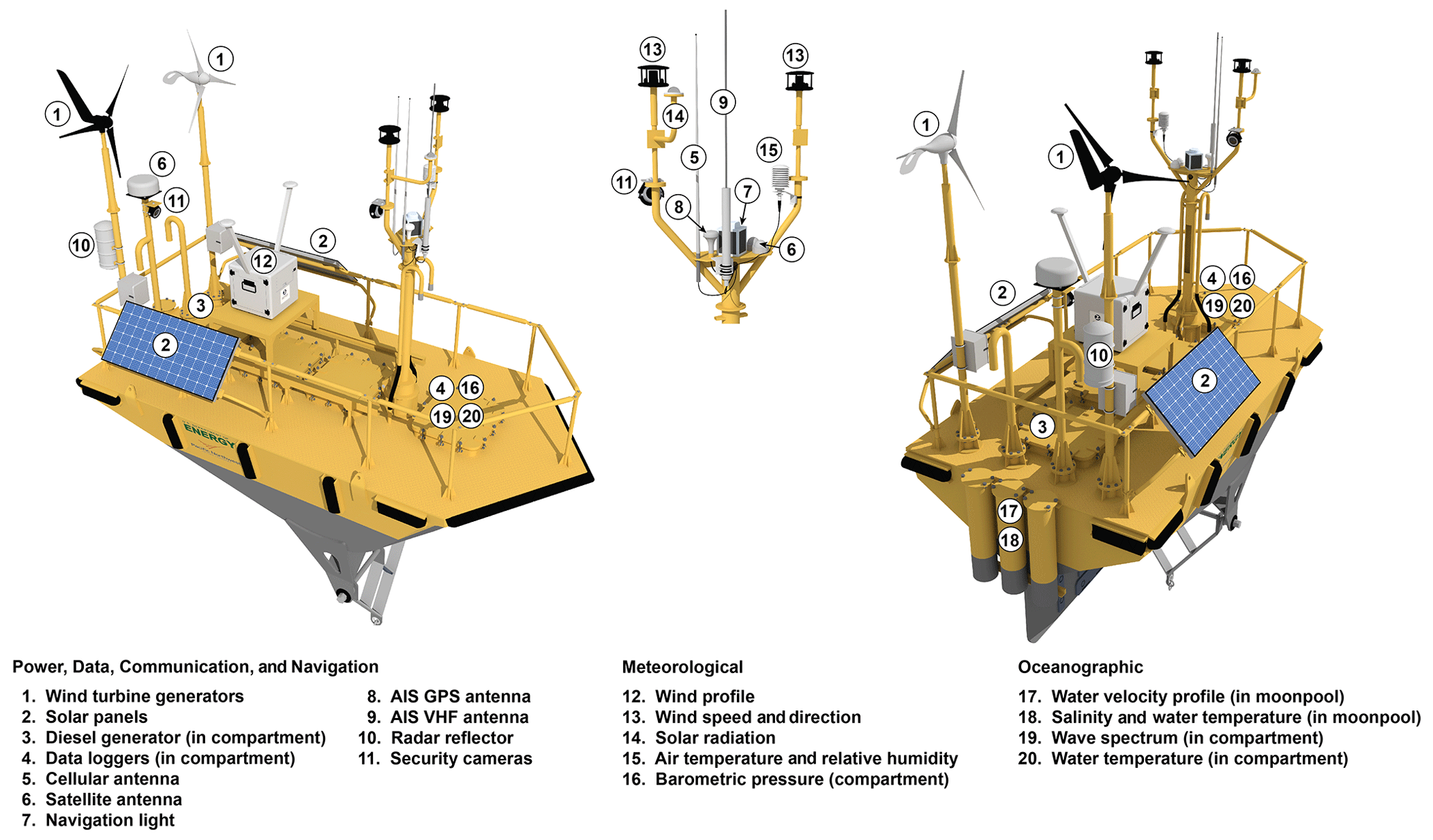
The DOE buoys used in this study have state-of-the-art instrumentation to measure the offshore wind resource. The buoys were procured as AXYS WindSentinel™ buoys in 2014 but have been significantly altered and upgraded since their initial procurement. The buoy hulls are identical to those of Navy Oceanographic Meteorological Automatic Device (NOMAD) buoys, which are known to be durable and to have good performance characteristics. They are also the principal hulls that were used on NDBC stations deployed off US coasts prior to the shift in use to discus buoys. The DOE buoys have aluminum, boat-shaped hulls (see Fig. 1 below) that are 6.1 m (20 ft) long and 3.0 m (9.8 ft) wide with a depth of 2.5 m (7.0 ft). A stainless-steel mooring yoke holds the buoy to its mooring. The yoke allows the buoy to rotate about the pitch axis but prevents the buoy from roll rotation (Timpe and Van de Voorde, 1995).

The mast on the bow of the buoy supports a satellite antenna, navigation lights, an AIS GPS/VHF antenna, a cup-and-vane anemometer (4.1 m a.s.l.), an ultrasonic anemometer (4.1 m a.s.l.), an air temperature and relative humidity sensor (3.7 m a.s.l.), and a solar radiation sensor (4 m a.s.l.). A radar reflector is placed at the stern of the buoy, and a wind profiler is placed mid-buoy deck that captures winds from 40 to 250 m a.s.l. In addition to atmospheric instruments, the buoy supports several oceanographic measurements, including sea-surface temperature measurements, an acoustic Doppler current profiler that provides ocean current speed and direction from the surface to 200 m water depth, a directional wave sensor, sea conductivity, and multiple inertial motion units to register buoy movements necessary for accurate wind calculations. Table 1 lists all the instruments, their make/model, and measurements provided by the DOE buoy during the California deployment (for more details on instruments, see Severy et al., 2021). The instrumentation on both buoys was identical. Deployment and maintenance of the buoys and instrumentation, as well as some post processing, were performed by AXYS Technologies through a subcontract from PNNL.

Figure 1 The three-dimensional schematic of the DOE buoy and sensor placement.

Table 1 Description of instrument manufacturer and models.

2.2 Instrument calibration and validation

The three inertial measurement units (IMUs) aboard the buoy were calibrated using a swing test where the buoy was rotated several times while suspended from a crane. The swing test was conducted on shore prior to deployment in the water. All IMUs recorded similar roll, pitch, and yaw measurements at different temporal resolutions (sample data shown in Appendix C for the Humboldt site). The GX3-25 IMU measured pitch, roll, and yaw at 1 Hz, while the GX5-45 and WindCube in-built IMUs measured at 10 Hz. The GX5-45 also provided measurements of linear velocity, angular velocity, and acceleration at 10 Hz, as well as position and velocity data at 4 Hz (Severy et al., 2021). The GX5-45 IMU data are used for motion-compensating the lidar wind speed, direction, and turbulence measurements. Before the California deployment, independent performance verification of both floating lidars was conducted at the Martha's Vineyard Coastal Observatory by DNV GL Energy USA Inc. (DNV GL). This verification was performed against a fixed, industry-accepted reference lidar. Wind speed and wind direction were compared against corresponding key performance indicators and acceptance criteria using the method provided in the roadmap toward commercial acceptance (Carbon Trust, 2018). In summary, both lidars (buoy nos. 120 and 130) demonstrated their ability to produce accurate wind speed and direction data. The lidar wind speed uncertainties were calculated to be less than 2 %, and correlation coefficients against the reference lidar wind speeds were greater than 99 %. A summary of the validation can be found in Gorton et al. (2020), and the validation report is available to the public on the PNNL buoy web page. (https://www.pnnl.gov/projects/lidar-buoy-program/technical-specifications, last access: 14 September 2023).

2.3 Field deployment summary

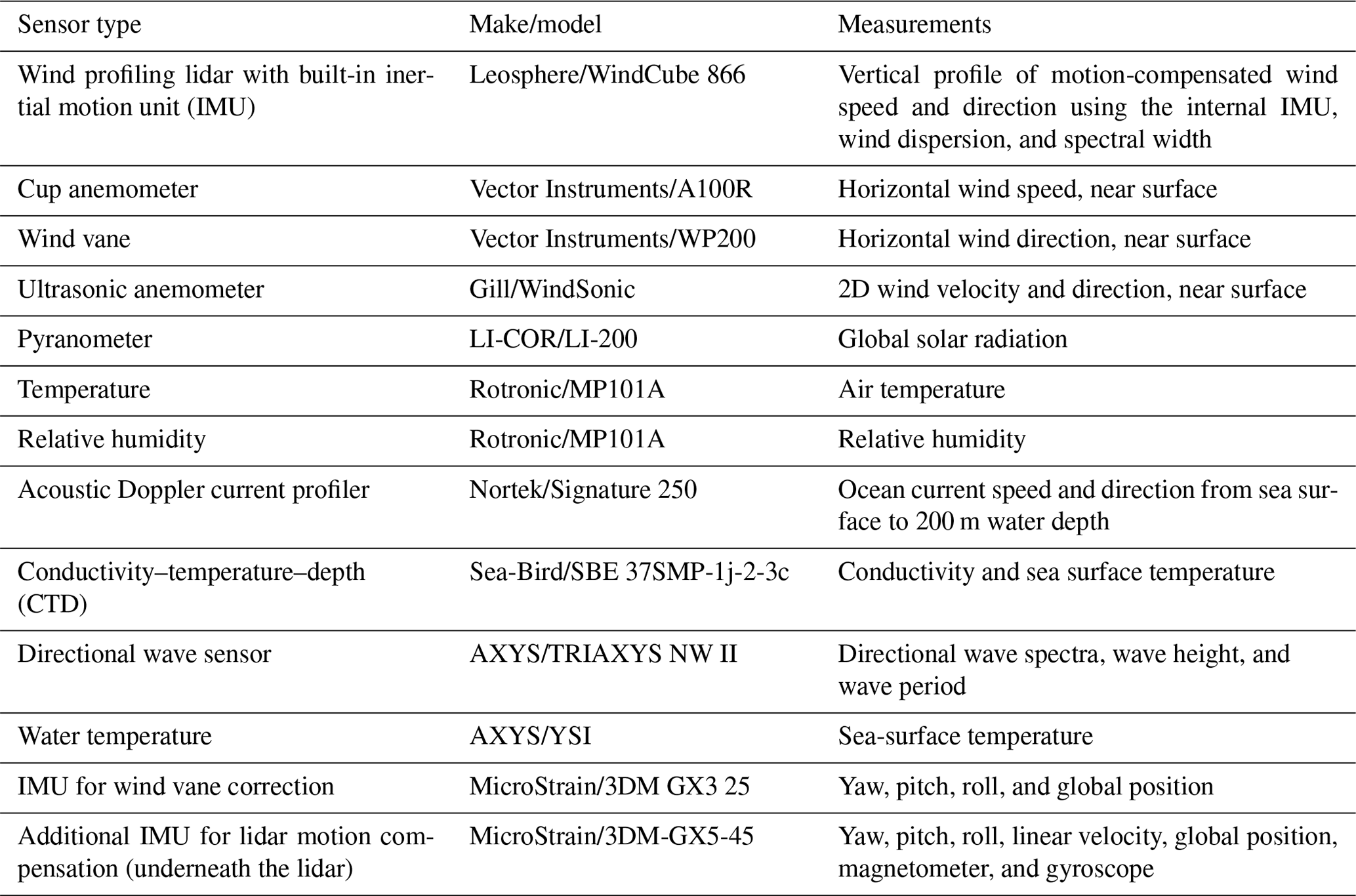
Figure 2a shows the location of the two buoys deployed within the Morro Bay and Humboldt WEAs. Multiple NDBC buoys are also located several kilometers away from the buoy sites. The NDBC buoy data are a good reference to confirm that the DOE buoy data are consistent in near-surface atmospheric and oceanographic variables. The spatial variability of the atmospheric and oceanographic variables can be assessed by comparing the measurements from these stations. The Morro Bay buoy (buoy no. 130) was deployed offshore from 28 September 2020 to 16 October 2021. Before the deployment, all the onboard IMU sensors were calibrated using a swing test, but significant drift was observed in the internal IMU within the lidar. All IMUs recorded similar trends in pitch, roll, and yaw with no time delay observed. The buoy was towed and moored approximately 50 km off the coast at approximately 35.71074^∘ N, 121.84606^∘ W. The buoy was deployed at 1050 m of water depth. The excursion radius was 1256 m with a mooring length of ∼ 1640 m. Figure 2c shows the final deployment picture of the Morro Bay buoy. At Humboldt, the buoy (buoy no. 120) was deployed offshore on 8 October 2020. The buoy was towed and moored approximately 40 km off the coast at approximately 40.9708^∘ N, 124.5901^∘ W. The buoy was deployed at a water depth of 575 m with a mooring length of 1050 m and an excursion radius of ∼ 800 m. Figure 2b shows the final deployment picture of the Morro Bay buoy. The raw and averaged data from the buoy were sent in near real time to the Wind Data Hub each day.

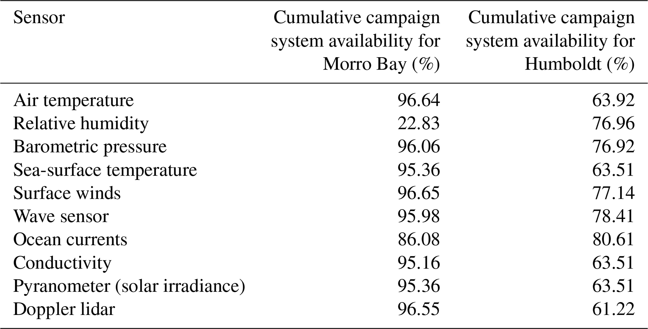
Figure 3 shows the instrument uptime for various sensors aboard both buoys, and Table 2 shows the cumulative campaign data availability for each sensor. Overall, the uptime of the buoy at Morro Bay was ∼ 98 %, and at Humboldt it was 91 % (ignoring the time when the buoy was turned off due to damage to the buoy's power system, discussed below). Sensors aboard the Morro Bay buoy performed adequately throughout the deployment and did not need a service visit or intervention. At Humboldt, the buoy unfortunately suffered some data loss due to challenging weather conditions. On 8 December 2020, the buoy encountered a large wave event off Humboldt County that resulted in damage to the buoy's power systems. To avoid additional issues, the buoy was remotely shut down until it was recovered for repair. Due to unfavorable weather conditions and other unforeseen delays, the buoy was redeployed on 24 May 2021 at 20:30 UTC. The buoy continued to experience power system issues which were ultimately resolved during a service visit on 9 April 2022. The Doppler lidar data had spotty availability during this period, because the lidar was turned on only during forecasts with high winds, i.e., when it could be powered solely by renewable sources. Finally, the Humboldt buoy was decommissioned on 28 June 2022 at 13:30 UTC.

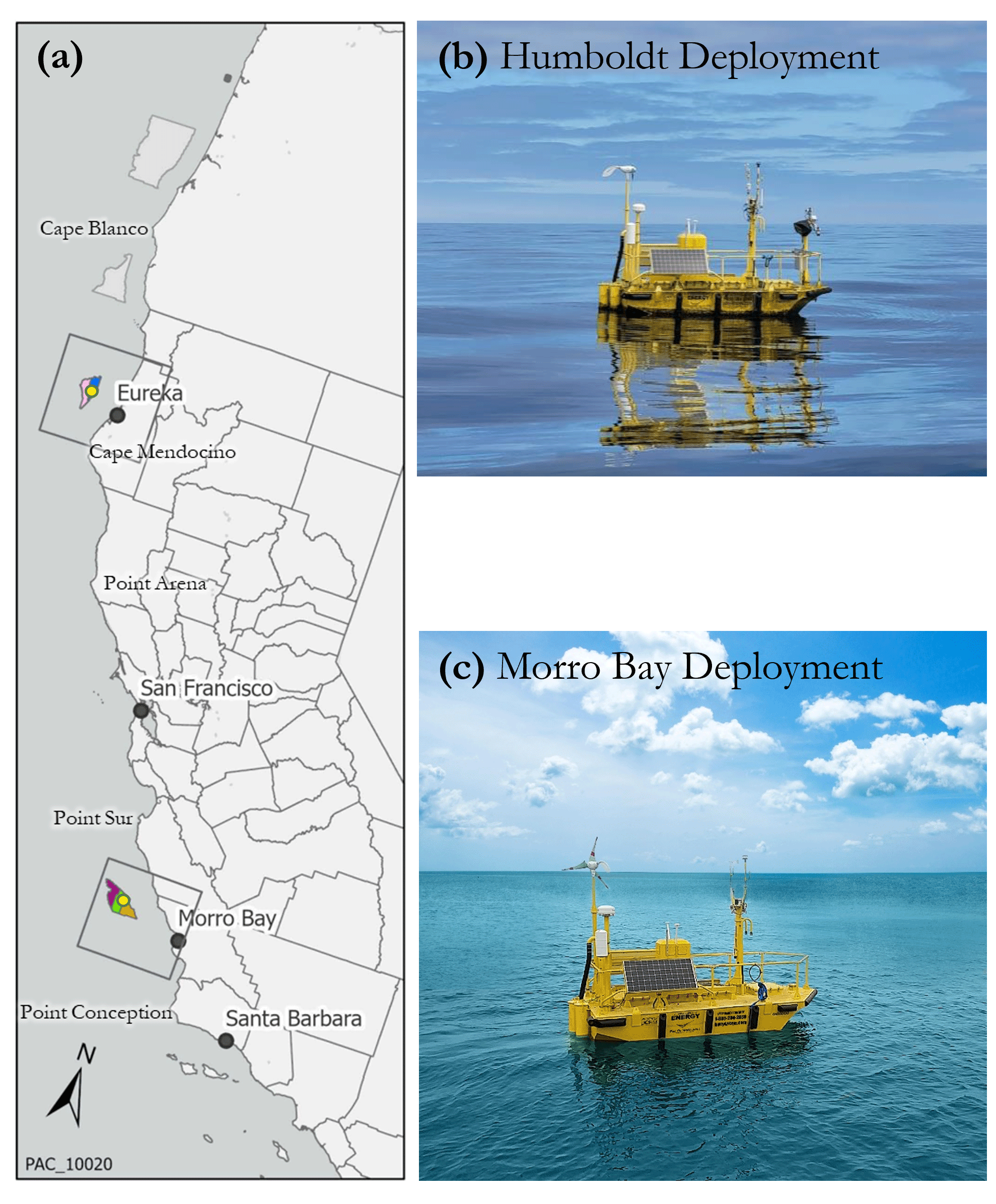
Figure 2 (a) The yellow circles indicate the location of the two buoys within the California wind energy lease regions (color coded, courtesy of BOEM). (b) A picture of the Humboldt buoy deployment in October 2020. (c) A picture of the Morro Bay buoy deployment in September 2020. Photos courtesy of AXYS Technologies, Inc.

Figure 3 (a) Instrument uptime at Morro Bay for various instrument sensors and (b) instrument uptime at Humboldt for various sensors.

Table 2 Cumulative campaign data availability after preliminary post-processing of the raw data from each sensor.

The Doppler lidar was configured to measure at predetermined heights or “range gates.” The height of the lidar window above mean sea level (m.s.l.) is 2.350 m. Therefore, for the actual measurement height, the range-gate configuration must be added to the height of the lidar window above m.s.l. The range gates were configured at 40, 60, 80, 90, 100, 120, 140, 160, 180, 200, 220, and 240 m relative to the lidar window.

3 Data analysis

Buoy measurements undergo standard quality checks, such as making sure the sensor is not providing data beyond manufacturer limits, detecting abnormal spikes in the data, filtering based on signal-to-noise ratio for the lidars, etc. These automated checks do not necessarily filter all bad data. This section describes the extra data quality checks, which include instrument cross-checking, physics-based analyses, and comparisons with nearby sensors. As a starting point, only data that were collected when the buoy was moored at the target location were considered in this analysis (any measurements collected during towing or services onshore were removed). Although measurements of pressure or temperature are valid when the buoy is moving, we mask them because they do not necessarily represent the conditions at the deployment location. Filtering by watch circle is performed in addition to instrument malfunction, the extent of the watch circle for both deployments is shown in Fig. 4. During the Morro Bay deployment, 490 measurements were flagged as bad, no measurement as questionable, and 52 083 as good. During the Humboldt deployment, 4461 were flagged as bad, 2 as questionable, and 68 312 as good. The two questionable measurements occurred when the buoy drifted a few tens of meters outside the watch circle but reported data within the watch circle during the previous and next measurements. The location data are also available within the surface data. A consolidated list of variables available in the post processed data is provided in Appendix B.

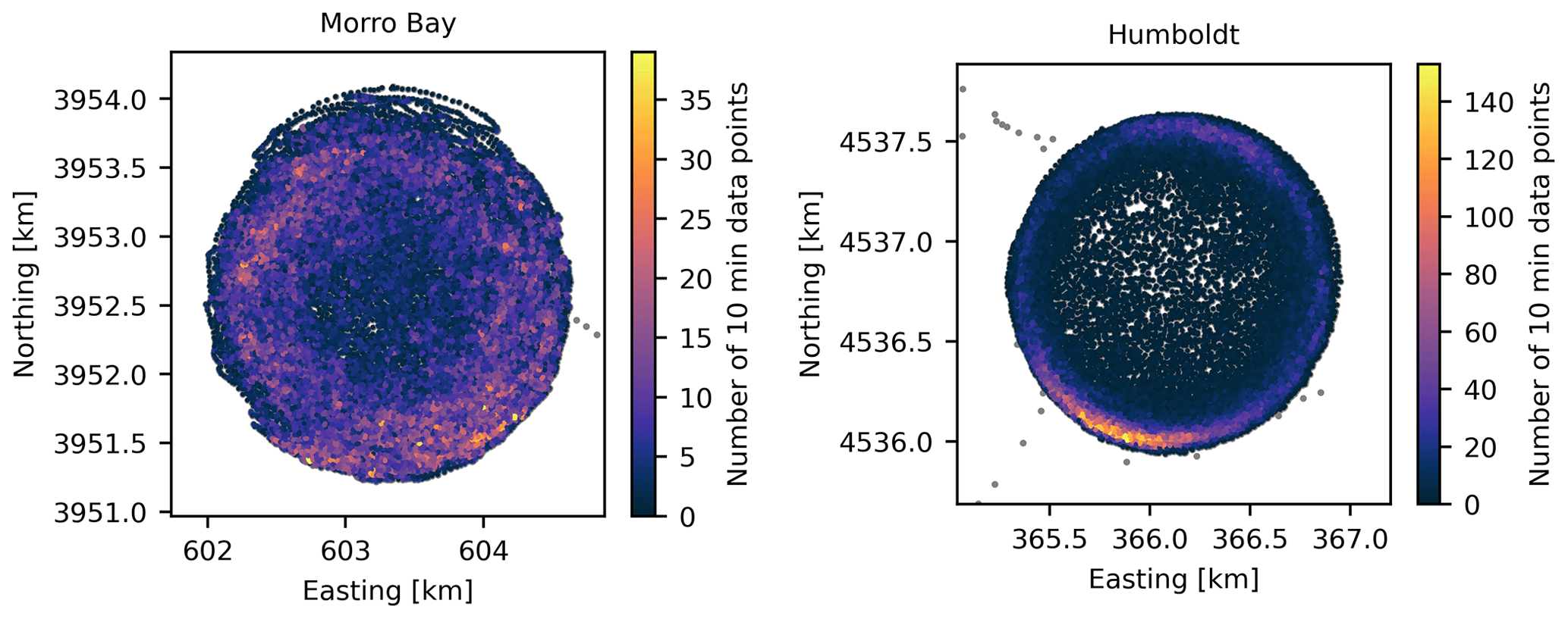
Figure 4 Location of lidar buoys during the deployments. Gray points have been identified as bad data. The color scale indicates the number of measurements in a 50 m² area. Data are projected in Universal Transverse Mercator zone 10.

3.1 Surface meteorological data processing and filtering

Each surface measurement (wind speed, wind direction, pressure, air temperature, and relative humidity) in the processed 10 min surface meteorological dataset was subjected to the following levels of quality analysis and filtration (Krishnamurthy and Sheridan, 2023a, c). First, if no instrument aboard the buoy (including the lidar, surface meteorological, and oceanic instruments) was reporting for a given timestamp, the event was considered a power outage, all surface measurements were assigned a value of NaN (not a number), and all surface measurement codes were set to 2; second, if an individual surface instrument was not reporting for a given timestamp but other surface instruments were reporting, the event was deemed an instrument failure and the individual surface measurement was assigned a value of NaN and a code of 3. Third, if no surface measurements were reporting but the lidar or oceanic instruments were reporting, the event was classified as a communications issue, so all surface measurements were assigned a value of NaN, and all surface measurement codes were set to 4. Fourth, individual surface measurements that were considered incorrect (atypical or unphysical) or outside the watch circle were filtered out by being assigned a value of NaN, and the corresponding individual surface measurement code was set to 5. Examples of atypical or nonphysical data include reported wind speeds less than 0 m s⁻¹, wind directions less than 0^∘ or greater than 360^∘, and relative humidity measurements outside the range of 0 % to 100 %. Any surface measurements that were physically probable but significantly diverged from nearby observations were assigned a code of 1. All remaining surface measurements were deemed good and assigned a code of 0.

The data recovery and quality of the surface meteorological observations during the Morro Bay deployment were high for all variables except relative humidity, with more than 90 % of the data designated as good (Table 3). Due to instrument failure, only 22.7 % of the relative humidity observations were deemed usable. For all surface meteorological variables, power outages, communications issues, and watch circle/incorrect data filtration affected the data recovery and quality for 0.8 %, 4.2 %, and 0.6 % of the Morro Bay deployment, respectively. Corrected near-surface wind directions were provided by AXYS and utilized in the Morro Bay near-surface b0 (final post processed data) dataset.

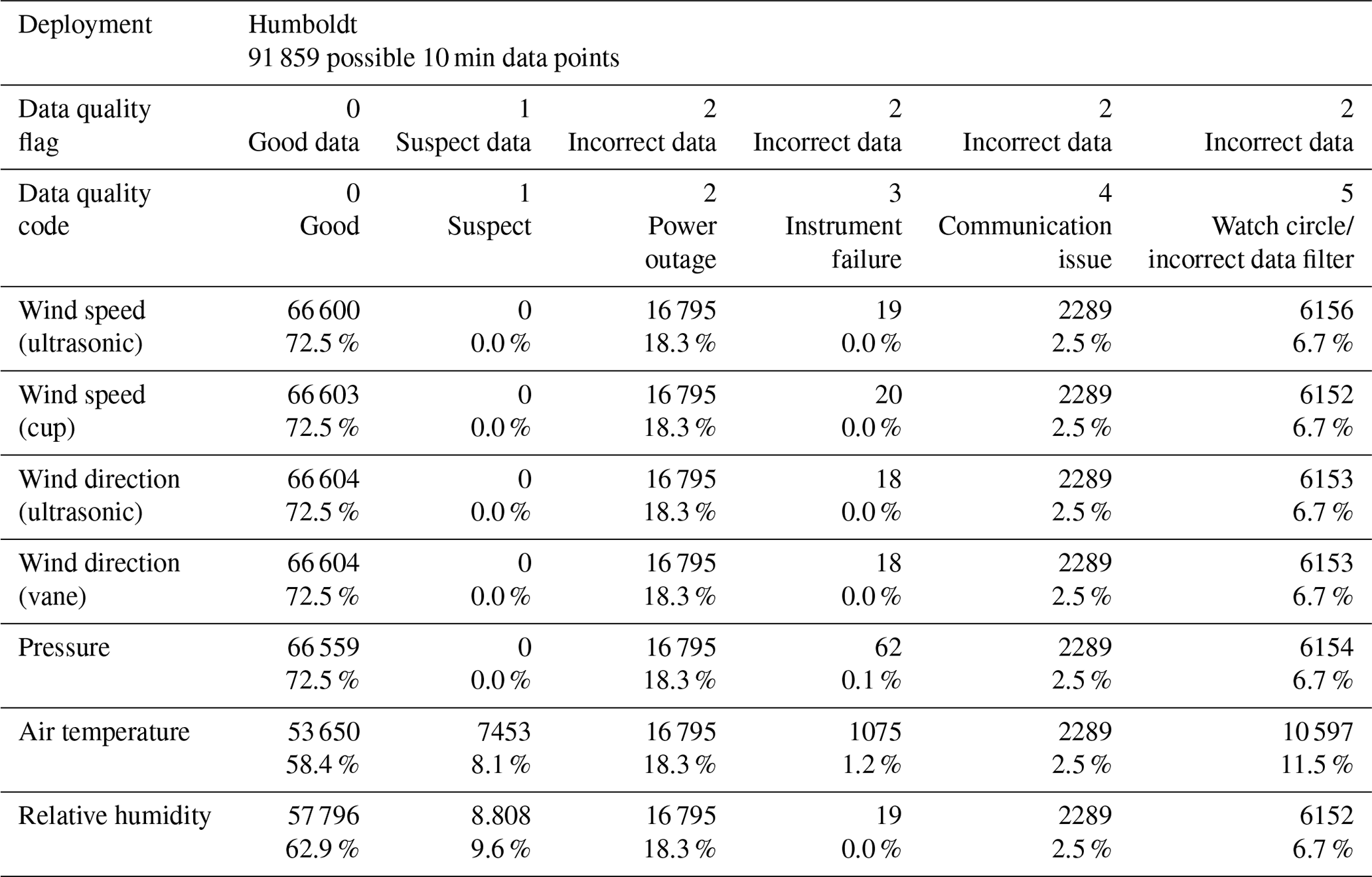
For the Humboldt deployment (Table 4), the data recovery and quality of the surface meteorological observations were both lower than at Morro Bay, even outside the extensive power outage periods discussed in Sect. 2.3. All surface instruments during the Humboldt deployment were subject to power outages for 18.3 % and communication issues for 2.5 %. Except for air temperature, the data recovery and quality for all surface meteorological variables were both affected by instrument failure for 0.1 % or less of the Humboldt deployment and by watch circle/incorrect data filtration for 6.7 % of the Humboldt deployment. No wind speed, wind direction, or pressure data were flagged as suspect, leaving 72.5 % of good data for these variables. Relative humidity observations during the period of 23 February 2022 to 29 April 2022 (9.6 % of the Humboldt deployment) were flagged as suspect due to atypical deviations from the nearest NDBC-buoy-derived relative humidity, leaving 62.9 % of good data. Missing air temperature observations due to instrument failure occurred during 1.2 % of the Humboldt deployment. In addition to the watch circle filtration, air temperature data at Humboldt were also filtered during four periods when the recorded measurements atypically dropped to around −30 ^∘C: 5–20 September 2021, 15–23 November 2021, 13 February 2022, and 24 February–5 March 2022. The total watch circle/incorrect data filtration for air temperature was 11.5 % at Humboldt. Air temperatures during the period of 5 March 2022 to 29 April 2022 (8.1 % of the Humboldt deployment) were flagged as suspect due to atypical deviations from the nearest NDBC buoy air temperatures, leaving 58.4 % of good data.

Table 3 Surface meteorological data quality flags for the Morro Bay deployment. The number of samples available after quality flag checks and percentage of data are also shown.

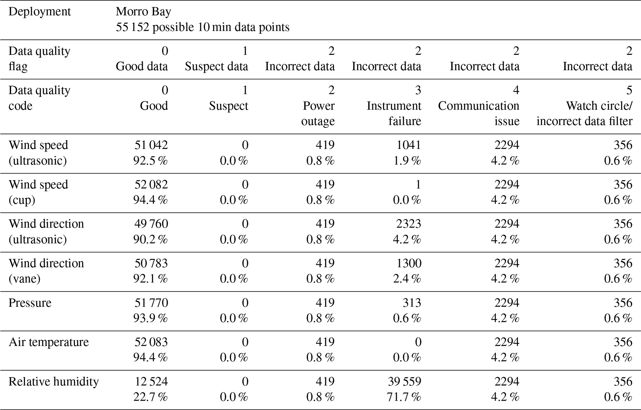
Table 4 Surface meteorological data quality flags for the Humboldt deployment. The number of samples available after quality flag checks and percentage of data are also shown.

3.2 Impact of motion correction on wind and turbulence estimates

Problems with the lidar internal WindCube IMU were known during the initial validation of the lidar. As a result, two backup IMUs were procured and installed on each lidar before the Morro Bay and Humboldt deployments. The backup IMUs were 3DM-GX5-45 (hereon referred to as the GX5) from MicroStrain Sensing. These devices were programmed to output platform attitude data at 10 Hz and position and velocity data at 4 Hz. Figures 5 and 6 show comparisons between roll and pitch measurements from the WindCube IMU and the GX5 at the Humboldt and Morro Bay sites, respectively. There is little agreement between the measurements from these two IMUs. The WindCube's measurements exhibit large fluctuations that are not physically realistic. Additionally, the WindCube's pitch and roll measurements show almost no correlation with the GX5 measurements. During the Humboldt and Morro Bay deployments, the WindCube lidar's motion-compensated wind estimates were affected by the internal IMU drift, which added significant noise to the 1 s motion-corrected wind profiles stored in real-time data files (*.rtd). Because these data are used to derive the final motion-compensated 10 min averaged data (i.e., the *.STA files), it is important to understand the impact of the bad WindCube internal IMU data on these results. Our approach involved reprocessing the uncorrected wind profiles using attitude data from the backup GX5-45 IMU unit. This allowed us to evaluate the impact of motion correction on wind speeds and velocity variances. The non-motion-compensated data are also available, which are referred to as the *.stdrtd (1 Hz) and *.stdsta (10 min averaged) files.

It is also important to note that, in addition to motion, the lidar's turbulence estimates are impacted by the sampling rate, range resolution, atmospheric conditions, and instrument noise (Frehlich, 1997; Sathe and Mann, 2013; Bodini et al., 2019a, b; Shaw et al., 2020; Kelberlau et al., 2020). In contrast to point sensors such as sonic anemometers, the lidar's ability to resolve very small-scale motion is affected by the laser pulse width and the pulse repetition frequency. More pulse averaging decreases the noise but lowers the sampling frequency. Shorter range gates (i.e., finer range resolution) result in degraded Doppler frequency resolution and greater uncertainty in the radial velocities, i.e., more noise. By contrast, longer range gates result in lower noise but smooth out the small scales. All these factors contribute to errors in the lidar-derived turbulence estimates.

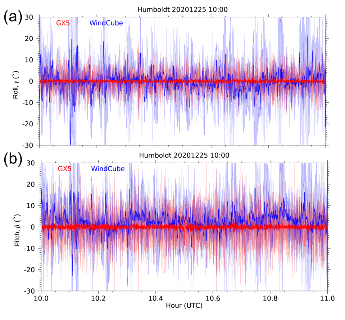
Figure 5 Comparison between the GX5 (red) and WindCube (blue) IMU measurements of (a) roll and (b) pitch observed on 25 December 2020, at the Humboldt deployment. Lighter shades show 1 s variability, and the darker shades show 10 s boxcar averages.

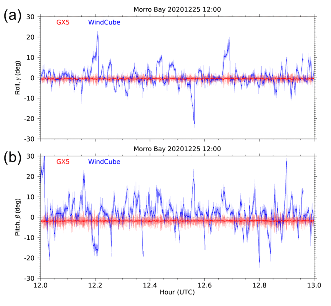
Figure 6 Comparison between the GX5 (red) and WindCube (blue) IMU measurements of (a) roll and (b) pitch observed on 25 December 2020, at the Morro Bay deployment. Lighter shades show 1 s variability, and the darker shades show 10 s boxcar averages.

The yaw measurements used in the WindCube's motion-correction procedure were derived from a differential GPS (DGPS) unit. There is good agreement between the GX5's magnetometer-derived measurement and the DGPS (not shown). The WindCube's motion-correction procedure uses its internal IMU for roll and pitch data and the DGPS for the yaw measurements to correct the 1 s winds. The final 10 min averaged results that appear in the *.STA files were obtained from averaging these 1 Hz data. Due to this fault in the WindCube internal IMU data, we observed an increase in turbulence and vertical velocity estimates in the WindCube 1 Hz STA data, as the true lidar beam observations are much closer to the respective beam azimuths and elevation angles than as estimated by the internal IMU data. This artificially induced motion results in overcompensating the 1 Hz data, creating a large error in turbulence estimates. We have observed that these impacts are canceled in a 10 min averaged wind speed estimate but are amplified when looking at turbulent statistics. Therefore, we recommend not using the WindCube STA files if interested in turbulence estimates from the lidars for these two deployments.

Reprocessing

Our approach involved reprocessing the uncorrected wind profiles using attitude data from the GX5 in place of the WindCube's internal IMU. We started with the uncorrected wind profiles that are stored in the *.stdrtd files. These files contain the x, y, and z components of the wind field (xwind, ywind, zwind) as measured in the WindCube's frame of reference. These measurements were obtained from Doppler beam-swinging (DBS) analysis of individual five-beam scans (Newman et al., 2016). Because these results were generated in real time, the DBS analysis was performed as each new beam came in. Thus, the *.stdrtd files were updated at the raw beam rate of ∼ 1.0 Hz. This resulted in considerable oversampling, because the true temporal resolution was determined by the scan time, which for the WindCube was about 5 s. Thus, the uncorrected wind profiles have a true temporal resolution of about 5 s but are oversampled at 1 s intervals. We adopted the same scheme for reprocessing the data to maintain consistency with the *.stdrtd files.

Motion correction

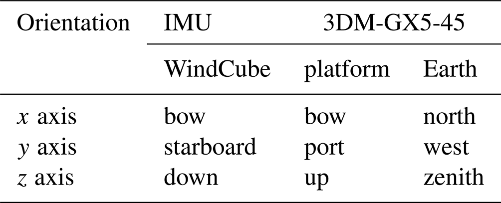
Figure 7a and b shows the coordinate system used by the WindCube and its orientation relative to the buoy. The WindCube instruments were installed on both buoys with their x axes pointing bow-ward and y axes pointing starboard. As a result, the WindCube instruments' z axes are downward. The 3DM-GX5-45's coordinate system is shown in Fig. 7c. This device was mounted upsidedown on the belly of the lidar with its x axis co-aligned to the lidar's x axis, i.e., toward the bow. As a result of the inverted orientation, the y axis of the 3DM-GX5-45 is pointed toward the port side, and z is up. The relationships between the WindCube and the GX5 coordinate systems are summarized in Table 5. Figure 7d shows the relationship between the Earth fixed reference coordinate system and GX5-45 coordinate system. The yaw angle (α) measures the orientation of the x^′ axis projected into the x–y plane, and the pitch angle (β) measures the orientation of x^′ relative the x–y plane. The roll angle (γ) describes a rotation about the negative x^′ axis, as indicated.

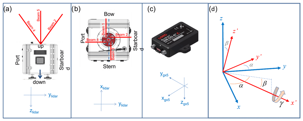
Figure 7 (a) Side view of the WindCube looking toward the bow, (b) top view of the WindCube, and (c) the 3DM-GX5-45 and its coordinate system. The x axis of the WindCube points toward the bow, and the y axis points toward the starboard side so that z points down. (d) The relationship between the Earth (x, y, z) and the GX5-45 (x^′, y^′, z^′) coordinate systems.

Table 5 Coordinate systems used by the WindCube and the 3DM-GX5-45 based on their installed positions during the Humboldt and Morro Bay deployments. The 3DM-GX5-45 provides measurements of the Euler angles necessary to transform from platform to Earth coordinates.

The uncorrected 1 s winds use the coordinate convention listed under “WindCube” in Table 5. The variables called “xwind”, “ywind”, and “zwind” in the *.stdrtd files correspond to the bow, starboard, and down directions, respectively. Transforming the WindCube's velocity measurements to the GX5 platform coordinate system simply involves taking the negatives of the WindCube's y and z velocity components, i.e.,

$$\begin{array}{}\text{(1)}& \left(\begin{array}{l}{v}_{\mathrm{bow}}\\ v_{\mathrm{port}}\\ v_{\mathrm{up}}\end{array}\right)=\left(\begin{array}{l}\mathrm{xwind}\\ -\mathrm{ywind}\\ -\mathrm{zwind}\end{array}\right).\end{array}$$

Each 1 s profile is transformed from WindCube coordinates to an Earth-fixed coordinate system using

$$\begin{array}{}\text{(2)}& \left(\begin{array}{l}{v}_{\mathrm{north}}\\ v_{\mathrm{west}}\\ v_{\mathrm{zenith}}\end{array}\right)=\mathbf{A}\left(\begin{array}{l}{v}_{\mathrm{bow}}\\ v_{\mathrm{port}}\\ v_{\mathrm{up}}\end{array}\right)\end{array}$$

where A is the matrix that transforms a vector from platform coordinates (in bow, port, up) to Earth coordinates (in north, west, zenith). A is given by

$$\begin{array}{}\text{(3)}& \mathbf{A}={\mathbf{R}}_{\mathbf{3}}\left(\mathit{\alpha }\right){\mathbf{R}}_{\mathrm{2}}\left(\mathit{\beta }\right){\mathbf{R}}_{\mathrm{1}}\left(\mathit{\gamma }\right)\end{array}$$

where α, β, and γ are the yaw, pitch, and roll angles, respectively. The individual rotation matrices are given by

$$\begin{array}{}\text{(4)}& {\displaystyle }{\mathbf{R}}_{\mathrm{1}}\left(\mathit{\gamma }\right)=\left(\begin{array}{lll}\mathrm{1}& \mathrm{0}& \mathrm{0}\\ \mathrm{0}& \cos \mathit{\gamma }& -\sin \mathit{\gamma }\\ \mathrm{0}& \sin \mathit{\gamma }& \cos \mathit{\gamma }\end{array}\right),\text{(5)}& {\displaystyle }{\mathbf{R}}_{\mathrm{2}}\left(\mathit{\beta }\right)=\left(\begin{array}{lll}\cos \mathit{\beta }& \mathrm{0}& \sin \mathit{\beta }\\ \mathrm{0}& \mathrm{1}& \mathrm{0}\\ -\sin \mathit{\beta }& \mathrm{0}& \cos \mathit{\beta }\end{array}\right),\text{(6)}& {\displaystyle }{\mathbf{R}}_{\mathrm{3}}\left(\mathit{\alpha }\right)=\left(\begin{array}{lll}\cos \mathit{\alpha }& -\sin \mathit{\alpha }& \mathrm{0}\\ \sin \mathit{\alpha }& \cos \mathit{\alpha }& \mathrm{0}\\ \mathrm{0}& \mathrm{0}& \mathrm{1}\end{array}\right).\end{array}$$

The order and direction of the rotations described by Eqs. (4) through (6) follow standard aerospace conventions as described in the GX5's documentation (Lord, 2019). When transforming from platform to Earth coordinates, a positive roll value results in port-side up and starboard down, which corresponds to a. right-handed rotation about the positive x axis. For the inverted GX5, a positive pitch corresponds to bow down and stern up, i.e., a right-handed rotation about the positive y axis (port-ward). Also, for the inverted GX5, a positive yaw corresponds to a counterclockwise rotation of the buoy, i.e., a right-handed rotation about the positive z axis (upward). In our case, Eqs. (3)–(6) represent the inverse transform from Earth to platform coordinates. As a result, R₁(γ) describes a rotation about the negative x axis, R₂(β), describes a rotation about the positive y axis, and R₃(α) describes a rotation about the negative z axis.

During reprocessing, we first computed the mean pitch, roll, and yaw from the GX5 over the pulse integration time of each lidar beam (∼ 1 s). This put the GX5 data on the same time grid as the lidar. We noted that the DBS analysis did not account for the variation in the platform attitude during the 5 s period it takes to complete one scan. Instead, we ignored motions with timescales shorter than the scan duration. Thus, for a given 5 s scan, the roll, pitch, and yaw were further averaged to produce the α, β, and γ values used in the transformation matrix, Eq. (3). We note that, in practice, there can be significant platform motion over the scan duration. Obviously, this will cause some error in the results. Averaging the 1 s data helps mitigate noise in the first-order moments (e.g., vertical velocity), but estimation of the second-order moments (e.g., vertical velocity variance) can be problematic. The final post-processed results are averaged like the STA files (Krishnamurthy and Sheridan, 2023b, d).

3.3 Wave observation data processing and filtering

Calculations of sea-surface gravity waves (henceforth waves) are derived from analyzing pitch, heave, and yaw over a 20 min time window in frequency space. A 20 min time window is the industry standard for wave measurements in the United States (NDBC, 1996). The 20 min sampling interval results in less wave data points than the rest of the instruments, which are sampled at 10 min intervals. Wave measurements are all derived from the TRIAXYS sensor, and the data were subjected to quality controls to identify spurious data by comparing measurements with adjacent ones and removing values of significant wave height exceeding 40 m (AXYS, 2012).

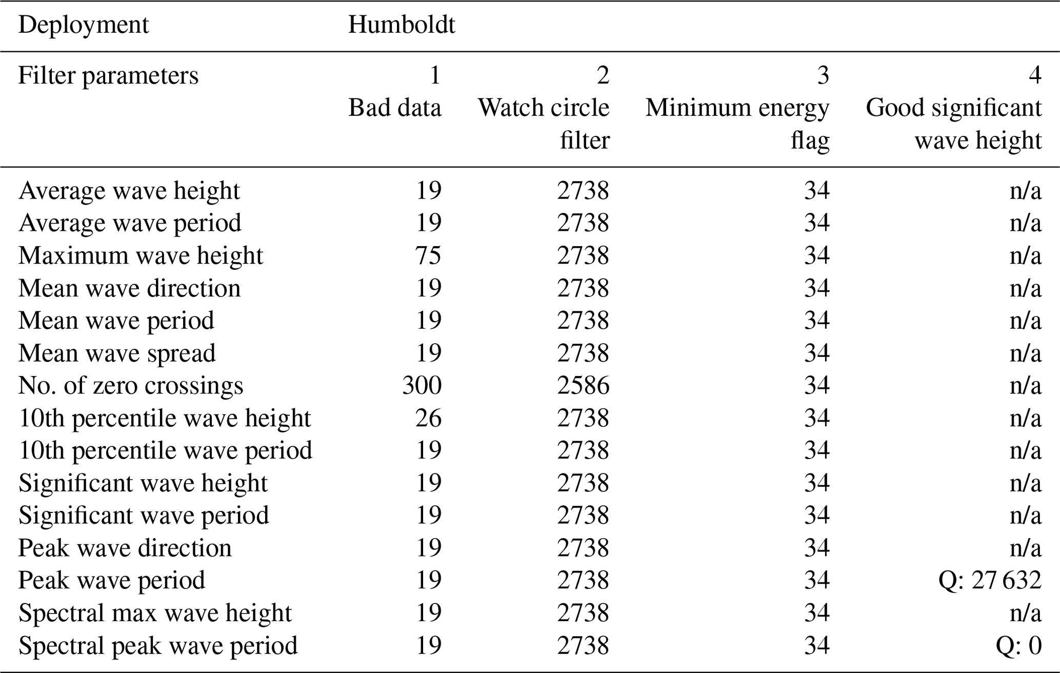
Like the surface measurements, only data within the watch circle were considered good. Thus, data marked as good or questionable outside of the watch circle by the first processing routines were marked as bad (Krishnamurthy and Sheridan, 2023a, c). Data from neighboring NDBC buoys were used as auxiliary to cross-verify the lidar buoy measurements. Stations 46028 and 46022 are located 7.7 and 25 km from the Morro Bay and Humboldt deployments, respectively. In addition, these buoys are deployed at depths of 1154 m (station 46028) and 419 m (station 46022), which are similar water depths to the lidar buoys and located far from prominent coastline features that would influence the waves. A wave climate similarity assessment was performed by pairing data flagged as good from the lidar buoys with NDBC data (the results are shown in Fig. 8). Linear regression shows slopes of 0.99 and 0.96 for the Morro Bay and Humboldt deployments, respectively – therefore, both buoy pairs experienced similar wave climates. The minimum significant wave heights measured during the deployment period at buoys 46028 and 46022 were 0.71 and 0.55 m, respectively. Therefore, significant wave heights less than 25 cm were flagged as unrealistic. A fourth level of filtering was applied to peak wave periods and peak wave direction based on significant wave height. If significant wave height was identified as questionable, then the peak wave periods and peak wave direction were as well. This only applies to questionable data, because bad data stem from sensor failure. Finally, if any of the variables were flagged as bad, then all were flagged as bad for that time period, because they were all derived from the same sensor. Summaries of the total number of current measurements with each quality flag are summarized in Tables 6 and 7.

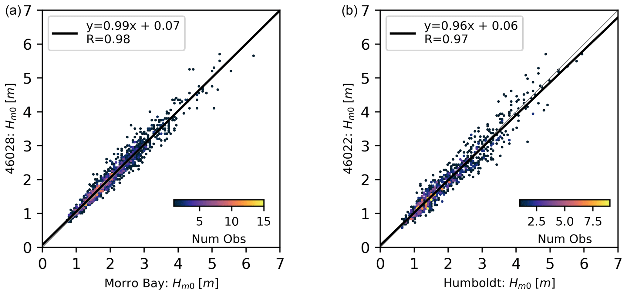
Figure 8 Significant wave height comparison between (a) Morro Bay and 46028 and between (b) Humboldt and 46022. Linear regression obtained using the least-squares method is shown in each figure along with the Pearson correlation coefficient. The color scales indicate the number of observations.

The spread between maximum wave height (H_max) and significant wave height (H_s) was also analyzed to investigate suspect data. H_s is defined as the average height of the highest $\mathrm{1}/\mathrm{3}$ waves in the sampling period. Wave heights have been shown to follow a Rayleigh distribution from which the maximum wave height in a record is estimated as $\mathrm{0.07}\sqrt{\ln \left(N\right)}{H}_{\mathrm{s}}$, where N is the number of measured waves. During the Morro Bay deployment, the maximum and average $H_{\max }/H_{\mathrm{s}}$ ratios were 2.5 and 1.6, respectively, when including questionable data, and they were 2.2 and 1.6 when considering good data only. Based on Rayleigh distributed waves, the expected values are 1.7 and 1.6 when including questionable data and 1.7 and 1.6 when considering only good data since N is not reduced significantly. This indicates that on average the data follow the expected distribution. In Morro Bay, only seven values from previously marked good data exceeded the $H_{\max }/H_{\mathrm{s}}=\mathrm{2.0}$ threshold – which has historically been used as a criterion for rogue waves (e.g., Müller et al., 2005; Nikolkina and Didenkulova, 2011) – and have thus been marked as suspect. In Humboldt, 18 points matched this criterion. None of these waves are the largest on the record – therefore, analyses based on extreme waves were unaffected.

Wave peak spread, wave duration, maximum wave period, and maximum wave crest were not included in the b0 file, because the instrument does not have the capability to measure them. Finally, the spectral peak wave period and peak wave direction were computed from the wave spectrum. The wave spectrum was estimated using the maximum entropy method (Nwogu, 1989) with the TRIAXYS post-processing software version 5.01. The spectral peak wave period is defined as the vertex of a parabola fitted to the maximum discrete period and its two adjacent periods in the directionally integrated spectrum. Peak wave direction follows the same procedure but with the frequency-integrated spectrum. These two variables do not contain data in the a0 file. Directions in the b0 file represent the direction where waves are coming from, measured clockwise from magnetic north.

Table 6 Data quality flags at the Morro Bay deployment. “n/a” represents not applicable, and Q represents quality samples.

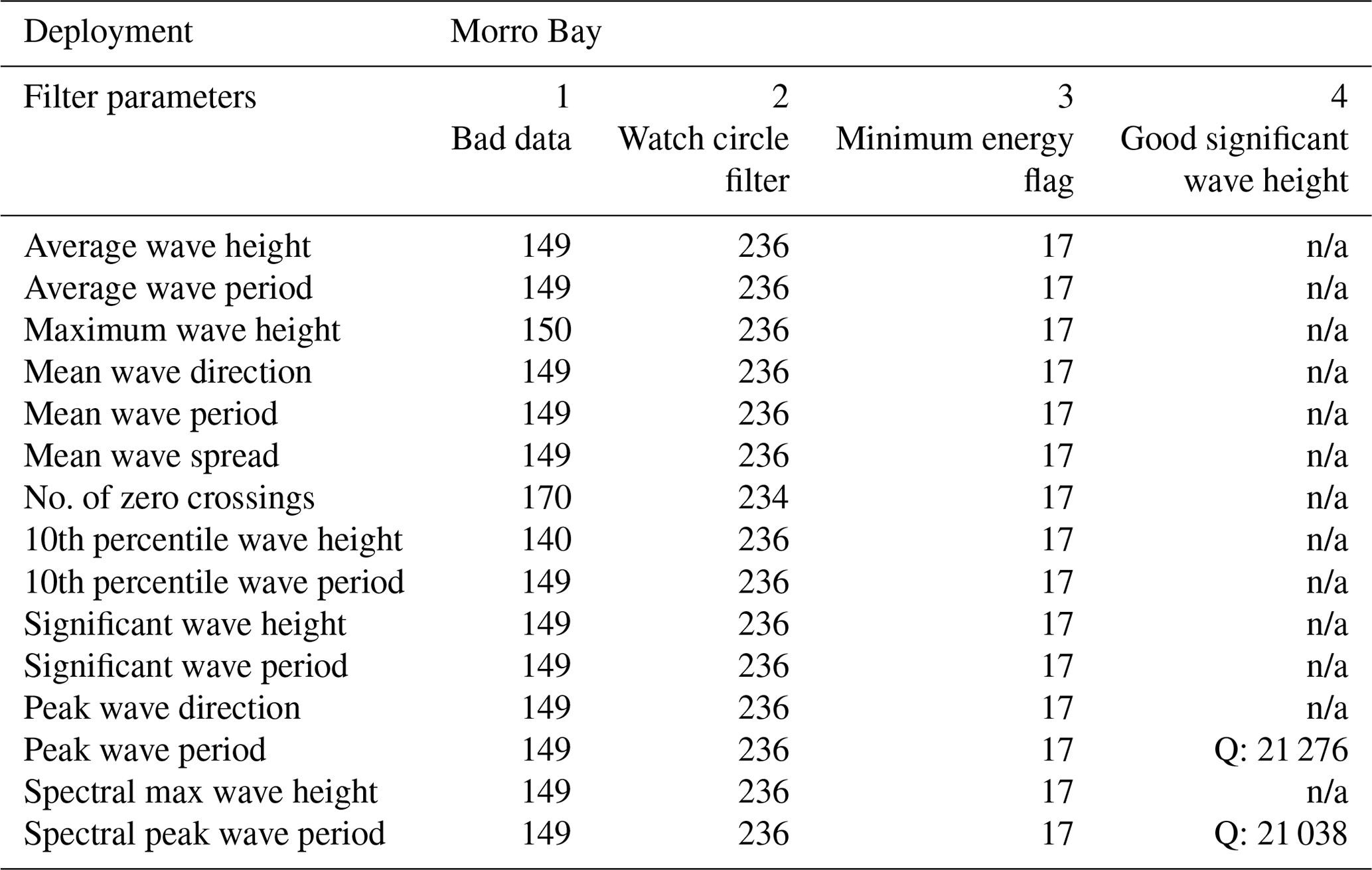
Table 7 Data quality flags at Humboldt deployment. “n/a” means not applicable, and Q represents quality samples.

3.4 Ocean current and CTD data processing and filtering

All the ocean current data were derived from the Nortek/Signature 250 acoustic Doppler current profiler (ADCP) in a 10 min window, and, as with the other sensors, were separated into three groups based on the data quality (Krishnamurthy and Sheridan, 2023a, c). The three groups included good, questionable, and bad data, with corresponding data quality flags of 0, 1, and 2, respectively. Like the filtering process in Sect. 3.4, watch circle masks were applied first, with only data within the watch circle considered good. For current speed, data that met any of the following conditions were marked as questionable:

• vertical shear of the current speed greater than 0.2 m s⁻¹,

• any data that were located between two NaN values in the vertical profile (missing values were marked as NaN),

• buoys that appeared just out of the watch circle once but then returned.

Data that met any of the following conditions were marked as bad:

• missing data;

• data from the last day before the number of bins in the ADCP changed – which included 6 October 2020 for the Morro Bay deployment and 28 December 2020 for the Humboldt deployment – to account for service visits;

• data from the last day of the deployment, which was 19 October 2021 for the Morro Bay deployment and 7 July 2022 for the Humboldt deployment;

• bursts of current speed that were temporally and spatially (in depth) uncorrelated and occurred only once (i.e., less than a 10 min duration);

• isolated measurement in time (i.e., measurements that did not have at least two consecutive successful events); and

• data measured during the buoy transit (i.e., outside the watch circle).

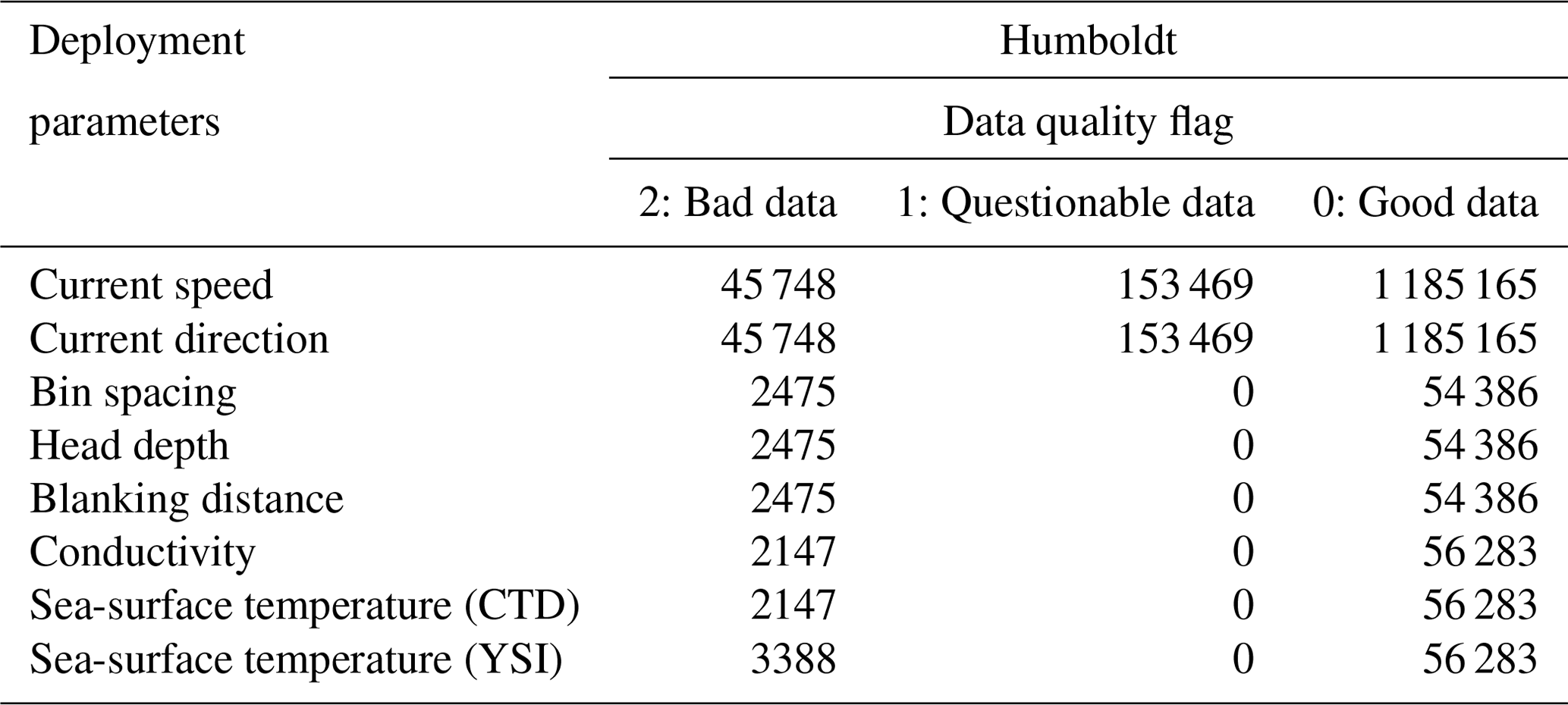
Summaries of the total number of current measurements with each quality flag are summarized in Tables 8 and 9. The maximum values among good data at Morro Bay and Humboldt were 2.01 and 1.45 m s⁻¹, respectively. The number of bins in the ADCP was initially set to 23 bins between 29 September 2020 and 6 October 2020, but then it was changed to 50 bins by 7 October 2020 at the Morro Bay deployment to improve the resolution of the data. On the contrary for Humboldt, there was an issue observed with the ADCP, so the number of bins was reduced from 50 to 23 after 28 December 2020.

Conductivity data were derived from the Sea-Bird CTD. Sea-surface temperature (SST) data were derived from two sensors, one from the Sea-Bird CTD measurement and the other from a YSI thermistor. Watch circle flags were also applied to filter the conductivity and SST data. At the Morro Bay deployment, the minimum and maximum SSTs from CTD among the good data were 9.940 and 19.149 ^∘C, respectively, and 10.002 and 20.385 ^∘C from YSI, respectively. In contrast, at the Humboldt deployment, the minimum and maximum SSTs from CTD among the good data were 9.544 and 18.300 ^∘C, respectively, and 9.524 and 18.796 ^∘C from YSI, respectively. Also note that the SSTs during the first 6 h from 29 July 2021 to 30 July 2021 at the Morro Bay deployment were marked as bad, because values from the CTD temperature sensor were unchanged during these periods. Summaries of the total conductivity and SST with each quality flag are also listed in Tables 4 and 5.

Table 8 Data quality flags at the Morro Bay deployment. The number of missing data points was not included in the second column.

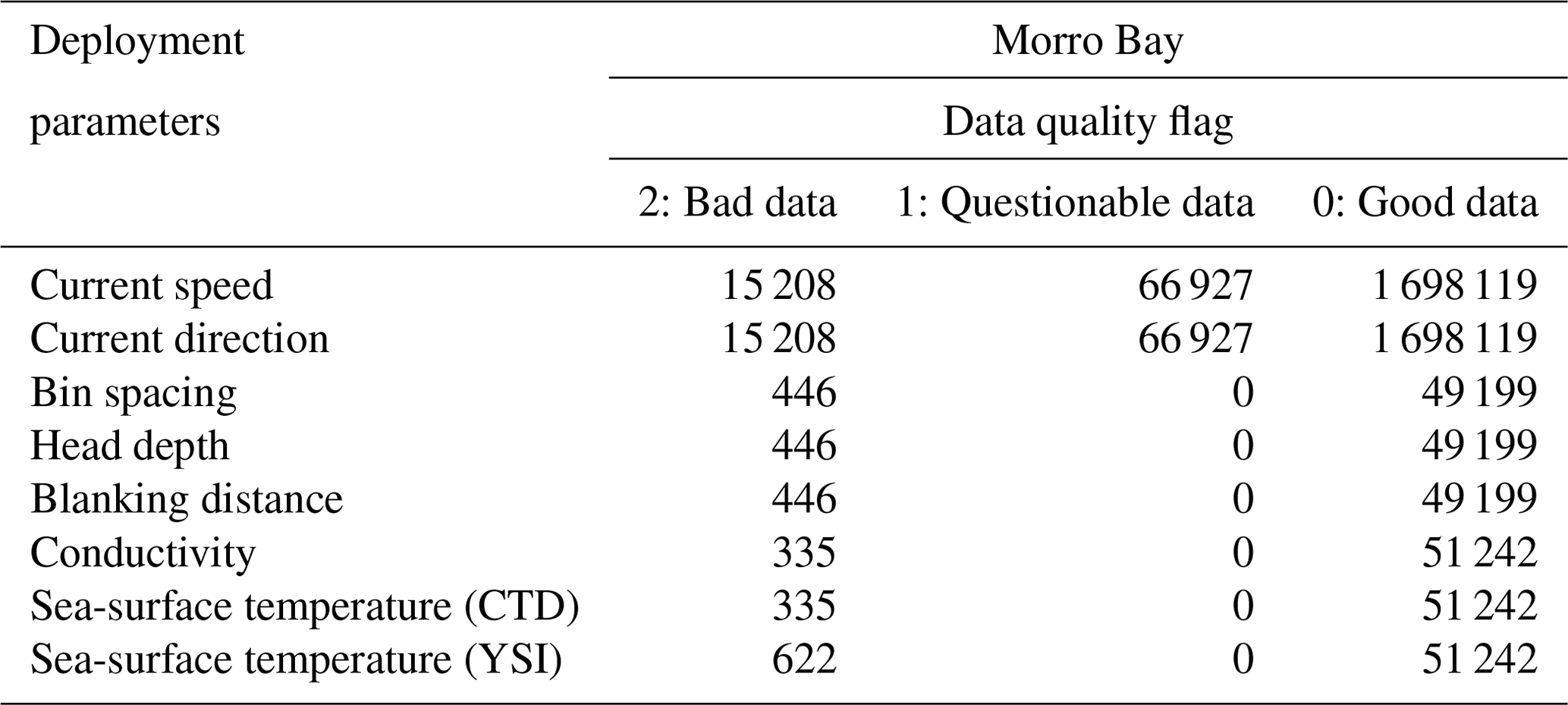
Table 9 Data quality flags at the Humboldt deployment. The number of missing data points was not included in the second column.

3.5 Pyranometer data processing and filtering

The two lidar research buoys each include a LI-200SA pyranometer (PYR) designed for field measurements of broadband global solar radiation (GSR). For the first time, the PYR-measured GSR was used here to assess both the presence of clouds and the “darkness” of the clouds. Our initial assessment was based on well-established methods developed previously for identification of clear-sky periods (Long and Ackerman, 2000) and cloud optical thickness (COT; Barnard and Long, 2004) from shortwave broadband data collected over land. It should be mentioned that the COT is a measure of sunlight attenuation passing through a cloud layer. Thus, the COT can be considered as a quantity for characterizing cloud darkness – clouds with large COT values (>10) have a “dark” appearance to a ground-based observer. The COT is related to cloud types (e.g., Rossow and Schiffer, 1991), which in turn are common markers of both dynamical and thermodynamic states of coupled atmosphere–ocean systems. Below is an outline of how these methods developed earlier for continental measurements can be extended to the more challenging coastal conditions.

During clear-sky conditions, identification of such conditions requires high-resolution (1 min) measurements of the global (or total) solar irradiance and its direct and diffuse components (Long and Ackerman, 2000). In contrast, the PYR-measured GSR has moderate resolution (10 min), and the required measurements of its direct and diffuse components are lacking. To address the lack of required inputs, changes of the GSR measured by PYR for a given day were monitored. The algorithm later checks for clear-sky periods that are long enough to allow for the corresponding empirical fitting to the diurnal cycle of sunlight described comprehensively by Long and Ackerman (2000). For example, a sufficiently large number (>100) of clear-sky points are required for empirical fitting of high-resolution (1 min) data (Long and Ackerman, 2000). Here, a limited number (>50) of clear-sky points was used for the empirical fitting of moderate-resolution (10 min) data. Coefficients of this fitting obtained for a given clear-sky day were used to estimate a hypothetical clear-sky GSR (Fig. 9a) for a nearby cloudy day. The term hypothetical is employed for the GSR that would be measured by PYR during clear-sky conditions for the considered cloudy day, i.e., an estimate is made of what the clear-sky GSR would be if the clouds were not present. Finally, the estimated values of clear-sky GSR were utilized to (1) calculate COT (Fig. 9b) using the method of Barnard and Long (2004) and (2) estimate a temporal cloud mask (Fig. 9c) by assuming that a given 10 min period is cloudy if the corresponding clear-sky GSR noticeably exceeds the PYR-measured GSR (>10 %). For our initial assessment, the selected threshold (10 %) is twice as large as the typical error (5 %) of the LI-200SA PYR under natural daylight conditions. The estimated temporal cloud mask can be used to calculate the average cloud amount for a longer period (e.g., 1 h) as a fraction of cloudy points blowing over the buoy location (Krishnamurthy and Sheridan, 2023a, c). Interpretation of the cloud mask should take into consideration the type of cloud present during the measured period. For example, dense fogs and plumes that occur in coastal areas may have optical thicknesses (up to 4) comparable to the COT of optically thin clouds, indicated by the horizontal magenta line in Fig. 9b. To distinguish dense fogs and plumes from optically thin clouds, additional measurements (e.g., lidar) are needed.

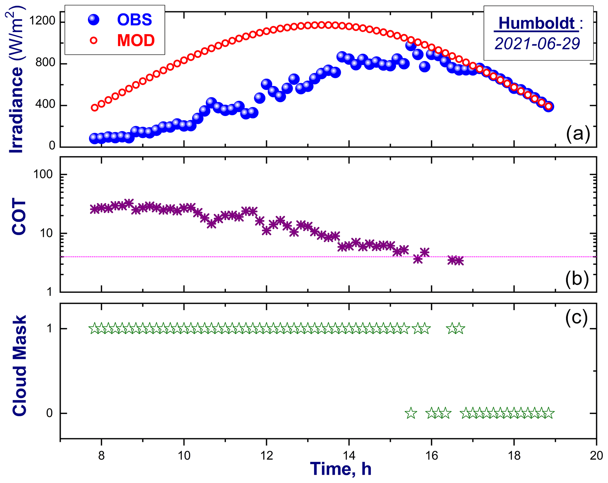
Figure 9 (a) The GSR measured (OBS) for a given day (29 June 2021) and location (Humboldt) and its estimated (or model) clear-sky (MOD) counterpart, (b) calculated COT, and (c) estimated cloud mask.

4 Results

4.1 Surface wind speed, direction, and temperature statistics

The two wind speed instruments aboard the buoys were in near-perfect agreement with each other during the Morro Bay and Humboldt deployments, with Pearson's correlation coefficients of 0.9996 and 0.9995, respectively (Fig. 10). Additionally, the near-surface wind speeds from the buoy deployments were also in good agreement with wind speed measurements from the nearest NDBC buoys during the deployment time periods, with correlations of 0.98 between the Morro Bay and NDBC 46028 buoys and of 0.91 between the Humboldt and NDBC 46022 buoys (Fig. 10).

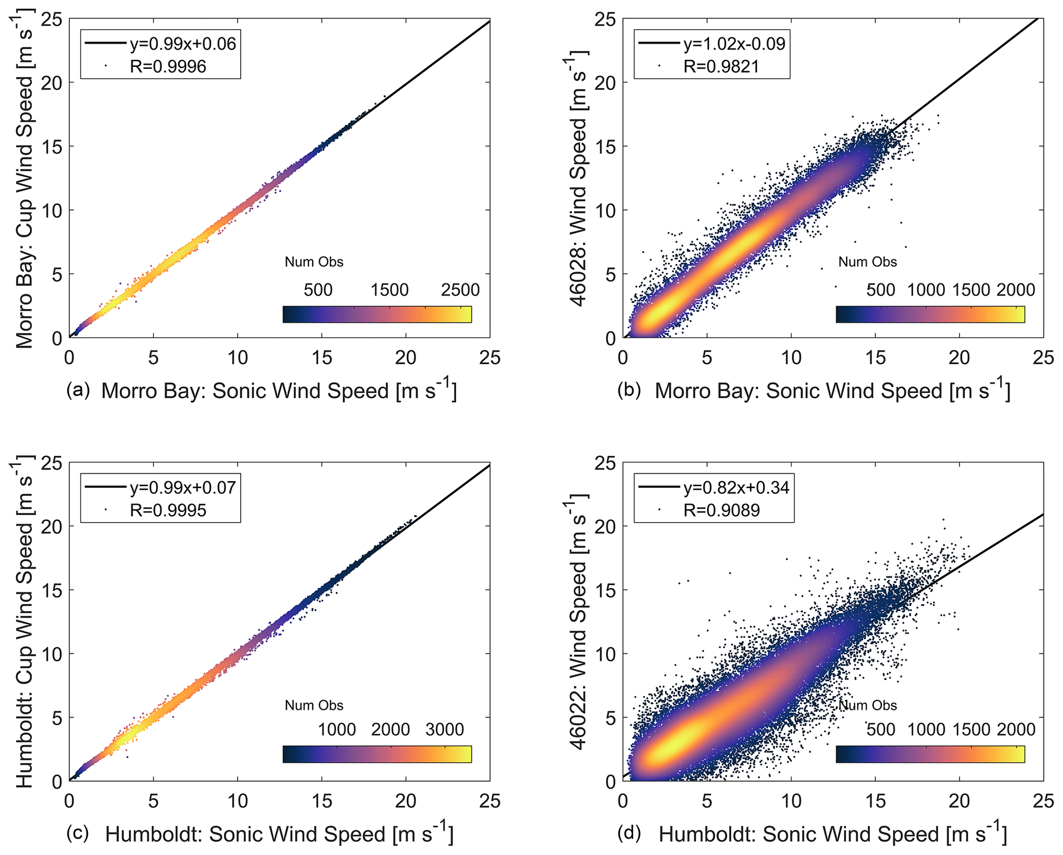
Figure 10 Onboard cup versus sonic near-surface wind speeds (a, c) and sonic versus nearest NDBC buoy near-surface wind speeds (b, d) at Morro Bay (a, b) and Humboldt (c, d).

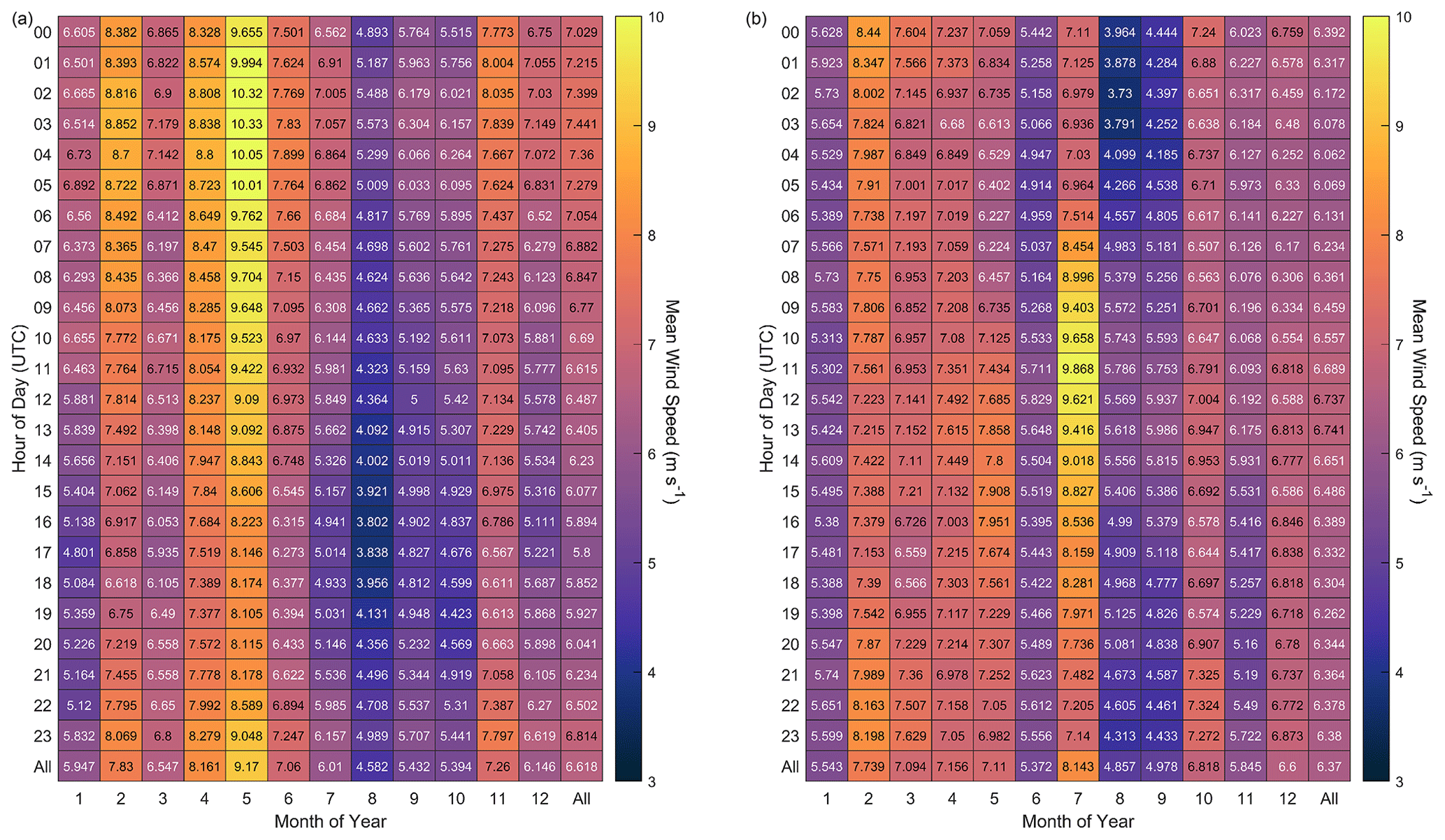
The 10 min averaged near-surface wind speeds have distinct seasonal and diurnal trends (Fig. 11). At Morro Bay, the fastest wind speeds, as averaged by hour of day over the month, occurred during the late spring, with a maximum of 9.17 m s⁻¹ in the month of May, and the slowest wind speeds occurred during the summer, with a minimum of 4.58 m s⁻¹ in the month of August. Diurnally, the fastest near-surface wind speeds occurred between 00:00–06:00 UTC, which corresponds with the evening transition in local time (16:00–22:00 Pacific standard time).

At Humboldt, a similar seasonal pattern to Morro Bay was observed with some of the fastest near-surface wind speeds occurring in the spring and the slowest occurring in late summer, with the distinct exception of the month of July. The fastest near-surface wind speeds at Humboldt, 8.14 m s⁻¹ on average, occurred during July, largely driven by the winds between 08:00–15:00 UTC corresponding with the middle of the night in local time (00:00–07:00 Pacific standard time).

Figure 11 Seasonal and diurnal average 4 m wind speeds at Morro Bay (a) and Humboldt (b).

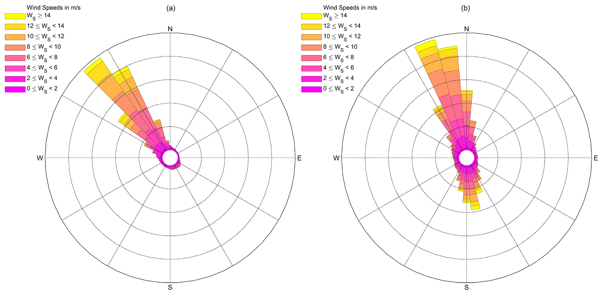
The near-surface wind direction distributions are predominantly uniform for each deployment, with the bulk of wind sourcing from the northwest at Morro Bay and the north-northwest at Humboldt (Fig. 12). Wind reversals are observed to occur along the United States Pacific coast (Bond et al., 1996), and infrequent occurrences of southeasterly near-surface flow were measured by the Morro Bay buoy, characterized by slow wind speeds. At Humboldt, more frequent occurrences of south-southeasterly flow were measured with a greater distribution of wind speeds during the events.

Figure 12 The 4 m wind roses at Morro Bay (a) and Humboldt (b).

Air and sea-surface temperatures show a distinct seasonal trend at Morro Bay (Fig. 13). Both temperatures are highest during the late summer and early autumn and lower in the spring. Temperatures at Humboldt also show a seasonal trend with a warmer summer and autumn and a cooler winter. The air–sea temperature difference (ΔT), in conjunction with wind speed, has been shown to be a good predictor for many processes in operational meteorology such as fog incidence and surface heat fluxes (e.g., Kettle, 2015). Performance of reanalysis models has been shown to correlate with atmospheric stability in the region (Sheridan et al., 2022). In Morro Bay, SST is on average higher than air temperature throughout the year (Fig. 13). Negative ΔT suggests higher likelihood of unstable atmospheric conditions at the site. In Humboldt, conditions often tend to be stable in the summer and unstable in the winter.

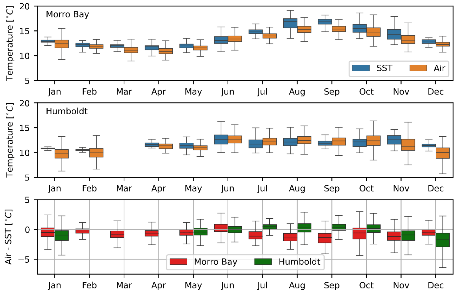
Figure 13 SST and air temperature at Morro Bay (a) and Humboldt (b). Air–sea-surface temperature difference (c). Data are shown for months with at least 2 weeks of data. The median monthly temperatures are indicated with the horizontal lines within each box, the 25th and 75th percentiles form the colored box range, and the minimum and maximum temperatures are displayed on the whiskers.

4.2 Doppler lidar wind speed, direction, and turbulence statistics

Ten-minute averages of wind speed, wind speed variance, wind direction, vertical velocity, and vertical velocity variance were computed from the corrected and uncorrected 1 s wind profiles. The 1 s data were quality controlled by assigning missing values to wind measurements with carrier-to-noise ratios (CNRs) below −23 dB. Within each 10 min interval, variances were computed by first linearly detrending the 1 s data (Krishnamurthy and Sheridan, 2023b, d). The data availability was also computed as the percentage of 1 s samples above the CNR threshold (−23 dB). No smoothing or interpolation (in height or time) was applied. To evaluate the impact of the motion-correction procedure, the effect on the median wind speed, turbulence intensity (TI), and vertical velocity profiles was examined. All the results shown in this section were obtained from the 10 min averaged data. Comparisons were carried out using only those time–height bins with mutually valid samples. This ensures that the median profiles are computed under identical meteorological conditions.

Figures 14 and 15 show the corrected wind speed and wind direction profiles for Humboldt and Morro Bay, respectively. Also shown are profiles of the difference between corrected and uncorrected wind speed profiles. The differences are quite small and indicate good agreement between the corrected and uncorrected results at all heights. Overall, the corrected wind speeds were about 3 mm s⁻¹ faster than the uncorrected winds at Humboldt, and at Morro Bay the differences are even smaller. This very close agreement indicates that it is possible to obtain accurate measurements of wind speed with no motion compensation whatsoever as long as one averages long enough. The lidar wind direction profiles shown in Figs. 14b and 15b indicate a strong preference for northwesterly flow at both Morro Bay and Humboldt. Both sites show no significant rotation with height. Morro Bay shows a strongly peaked distribution about 320^∘. Humboldt shows a dominant peak at about 345^∘ and a much weaker secondary peak near 160^∘. Also shown in Figs. 14a and 15a are profiles of the median wind speed profiles under stable and unstable atmospheric conditions. Here we define stable (unstable) conditions as whenever the air–sea temperature difference is positive (negative). The air–sea temperature difference was obtained from the difference between (model name) air temperature sensor at ∼ 4 m and the CTD water temperature sensor at a depth of 1 m. At Humboldt (Fig. 14a), the stable profile (blue) increases more rapidly with height and exhibits greater shear than the unstable (red) profile. At Morro Bay, wind speeds under stable conditions are higher at all levels, with slightly more shear than under unstable conditions.

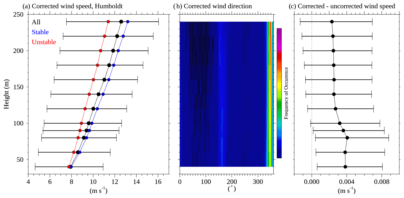
Figure 14 Humboldt observations showing (a) the median corrected wind speed profile (black), (b) the corrected wind direction distribution profile, and (c) the difference between the motion-corrected and uncorrected wind speeds. Also shown in panel (a) are the median wind speed profiles for periods with positive (blue) and negative (red) air–sea temperature differences. Error bars show the 25th to 75th percentile range. The results shown here cover the period from 25 May 2020 to 20 December 2020.

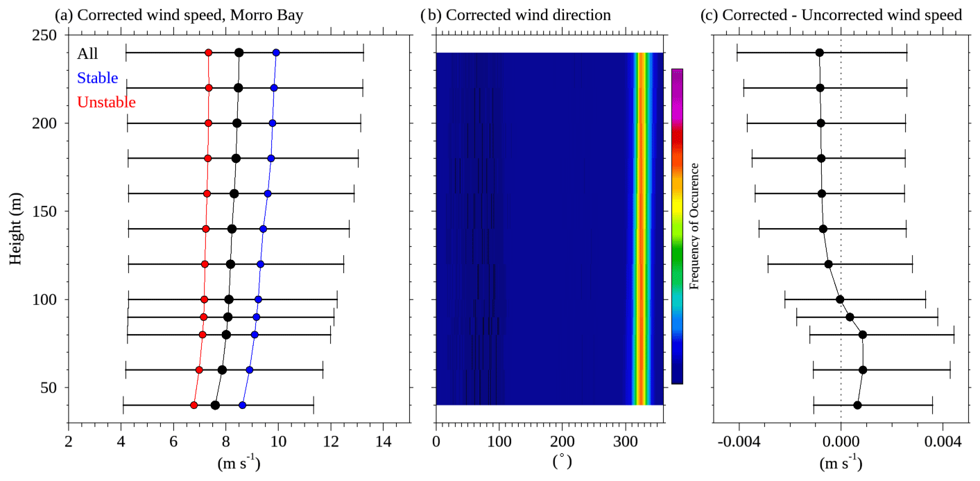
Figure 15 Morro Bay observations showing (a) the median corrected wind speed profile (black), (b) the corrected wind direction distribution profile, and (c) the difference between the motion-corrected and uncorrected wind speeds. Also shown in panel (a) are the median wind speed profiles for periods with positive (blue) and negative (red) air–sea temperature differences. Error bars show the 25th to 75th percentile range. The results shown here cover the deployment period from 17 October 2020 to 16 October 2021. The wind direction distributions shown in panel (b) are normalized at each height so that the sum of the distribution is one. The color bar scale runs from 0 to 0.05.

Figures 16 and 17 show the corrected TI profiles for Humboldt and Morro Bay, respectively. Also shown are profiles of the difference between corrected and uncorrected TI profiles. The TI was computed using wind speeds greater than 1 m s⁻¹. The TI differences are quite small and indicate good agreement between the corrected and uncorrected results at all heights. Overall, the uncorrected TIs were about 0.5 % larger than the corrected values at both Humboldt and Morro Bay.

Figure 16 Humboldt observations showing (a) the median corrected TI profile and (b) the median difference between the corrected and uncorrected TI. Also shown in panel (a) are the median profiles for periods with positive (blue) and negative (red) air–sea temperature differences. Error bars show the 25th to 75th percentile range. The results shown here cover the period from 25 May 2020 to 20 December 2020.

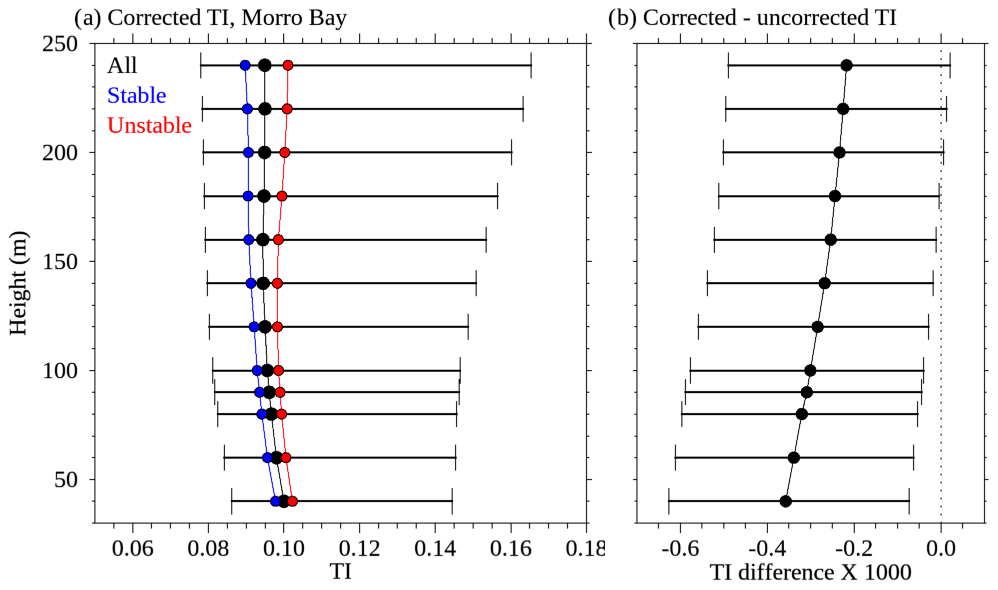
Figure 17 Morro Bay observations showing (a) the median corrected TI profile and (b) the median difference between the corrected and uncorrected TI. Also shown in panel (a) are the median profiles for periods with positive (blue) and negative (red) air–sea temperature differences. Error bars show the 25th to 75th percentile range. The results shown here cover the period from 17 October 2020 to 16 October 2021.

Figure 18 shows comparisons between corrected and uncorrected vertical velocity profiles for both Humboldt and Morro Bay. Since we expect the mean vertical velocity to be very close to zero, the vertical velocity can be used to evaluate the motion-correction procedure. Figure 18 shows that motion-corrected vertical velocities exhibited smaller biases at both sites compared to the uncorrected velocities. At Morro Bay the vertically averaged vertical velocity was −16 cm s⁻¹ for the uncorrected data and −13 cm s⁻¹ for the corrected data. At Humboldt, where the motion correction procedure had a more significant impact, the vertically averaged vertical velocities were −31 and −2 cm s⁻¹ for the uncorrected and corrected data, respectively.

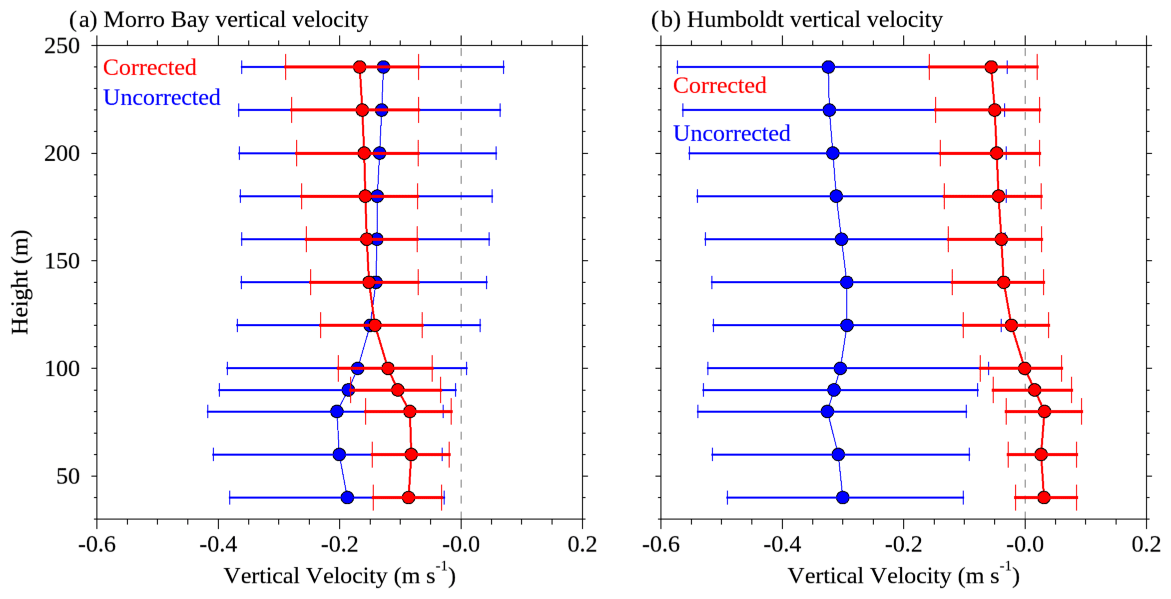
Figure 18 Median corrected (red) and uncorrected (blue) vertical velocity profiles for (a) Humboldt and (b) Morro Bay. Error bars show the 25th to 75th percentile range.

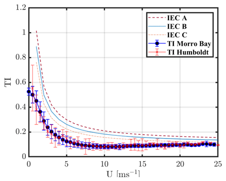
Figure 19 The 100 m bin-averaged TI estimates vs. average wind speeds at Morro Bay and Humboldt. The various International Electrotechnical Commission (IEC) wind-turbine-specific TI curves are also shown.

Figure 19 shows bin averaged TI for every wind speed bin at 100 m above sea surface level for both Humboldt and Morro Bay. The International Electrotechnical Commission (IEC) estimates for various turbine classes are also shown. This shows that floating offshore wind turbines off the US west coast will encounter low atmospheric turbulence, similar to the US east coast (Nicola et al., 2019). Profiles of lidar data availability (DA) during the Humboldt and Morro Bay deployments are shown in Fig. 20. The dataset uses missing values to flag samples that fall below a predefined CNR threshold. For the WindCube, that threshold was set at −23 dB. The data availability generally degrades with altitude, particularly above about 100 m a.g.l. Height-averaged DAs for Humboldt and Morro Bay were 83 % and 92 %, respectively. Data after 20 December 2021, from the Humboldt deployment, are currently under investigation due to an issue observed with the lidar data and are being diagnosed by the vendor.

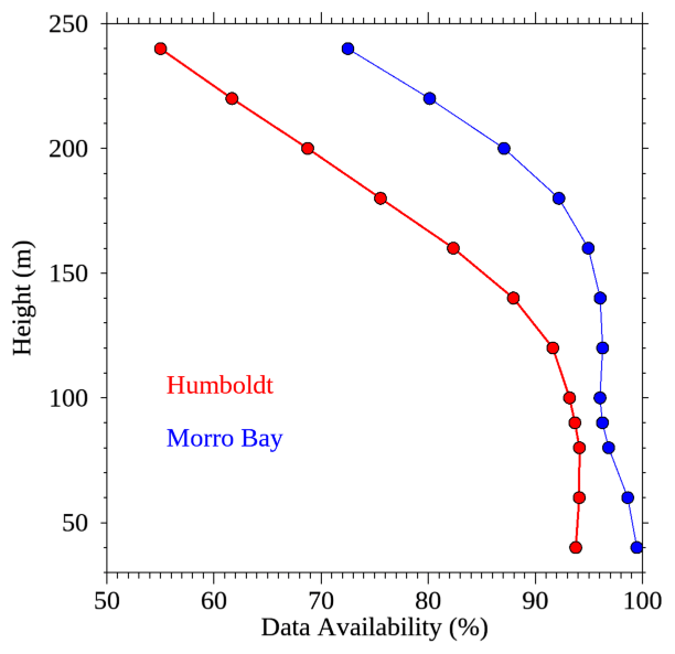
Figure 20 Data availability for the corrected lidar winds at Humboldt (red) and Morro Bay (blue).

4.3 Ocean current and direction statistics

The ocean currents had different spectra at the two buoy deployments, as shown in the wind rose (Fig. 21). Surface currents were more energetic at the Humboldt deployment than those at the Morro Bay deployment, which were more widely spread. At Morro Bay, the mean and median values of the measured surface current speed were 22.6 and 20.0 cm s⁻¹, respectively, and were 18.6 and 16.0 cm s⁻¹, respectively, for all measured current speeds. Of all currents, 10.7 % came from the southeast, and 41.2 % of the surface currents came from the northeast toward the southeast. This suggests that the mean kinetic energy peak changed between the surface and greater depths.

At Humboldt, the ocean currents came roughly from the same directions at the surface and at greater depths. For instance, approximately 26.7 % of all the currents and 35.3 % of the surface currents traveled north to northeast. The mean and median values were 28.1 and 26.0 cm s⁻¹ for the measured surface current speed, respectively, and 21.8 and 20.0 cm s⁻¹ for all measured current speeds.

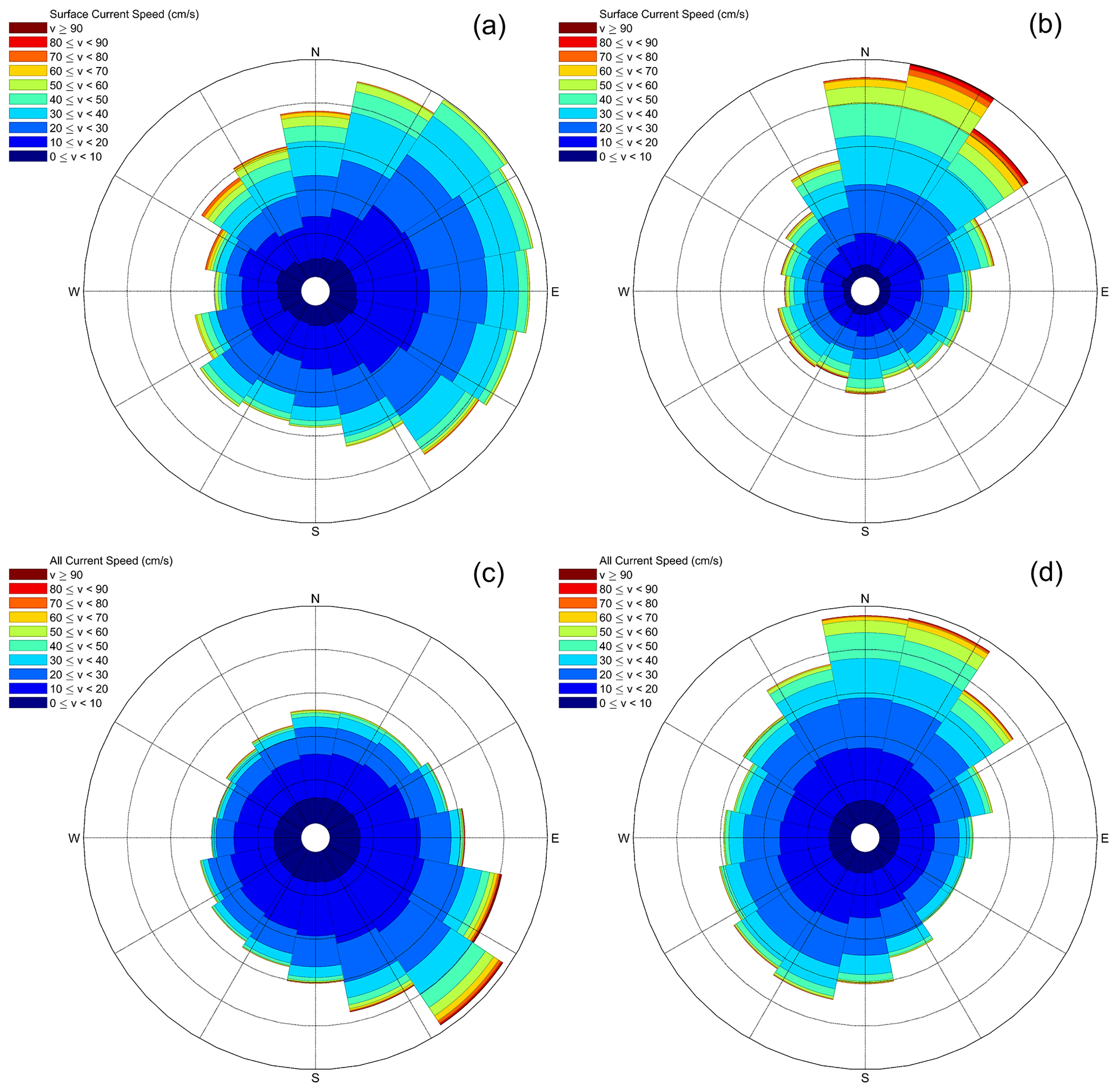
Figure 21 Wind rose of ocean currents at the surface (a, b) and at all depths (c, d) at both Morro Bay (a, c) and Humboldt (b, d). Only good data with quality control were included in the analysis.

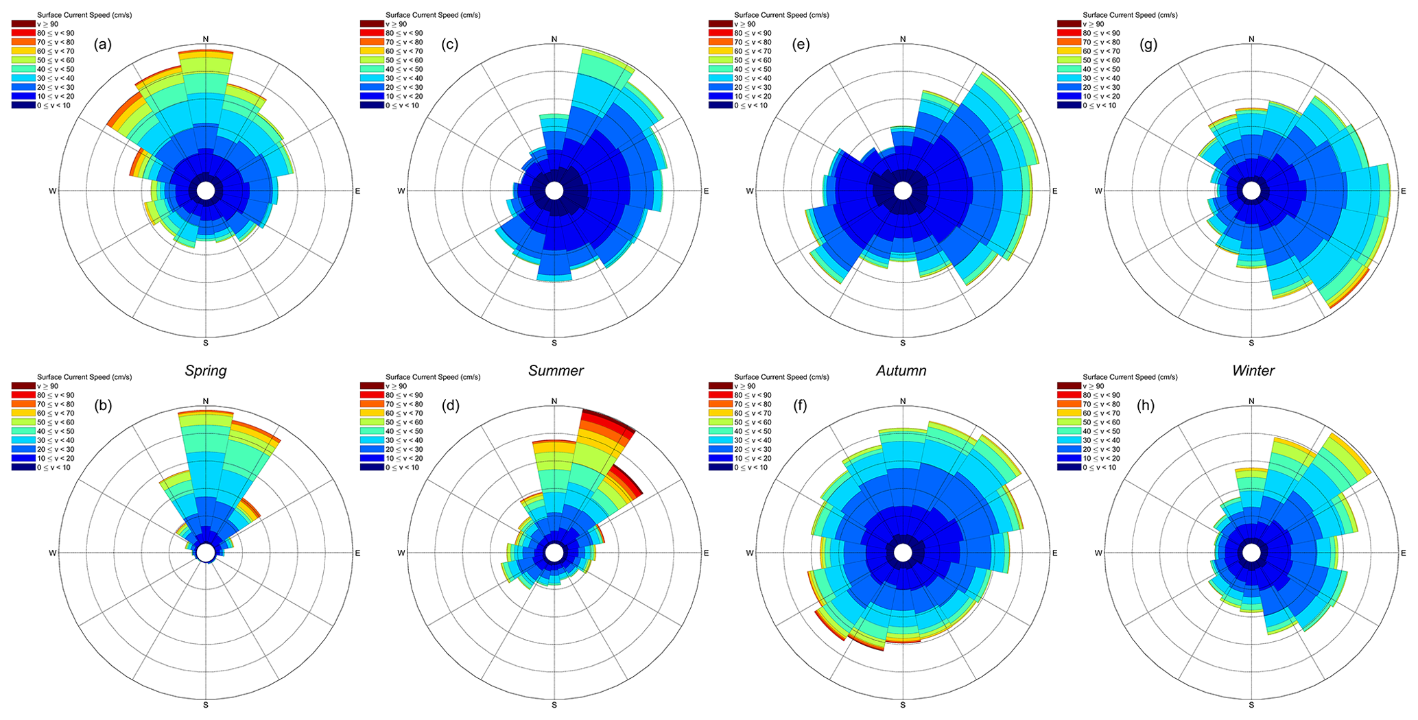
Figure 22 Wind rose of seasonal surface currents at Morro Bay (a, c, e g) and Humboldt (b, d, f, h). Only good data with quality control were included in the analysis.

There were strong seasonal variations in the surface current at both deployments (Fig. 22). The average surface current speeds during spring, summer, autumn, and winter at the Morro Bay deployment were 27.2, 18.0, 19.4, and 24.8 cm s⁻¹, respectively. At the Humboldt deployment, they were 33.3, 33.1, 25.0, and 25.5 cm s⁻¹, respectively. The mean surface current speeds during each season at the Morro Bay deployment were 25.0, 16.0, 17.0, and 24.0 cm s⁻¹. At the Humboldt deployment, they were 32.0, 30.0, 23.0, and 24.0 cm s⁻¹, respectively. The surface current at Morro Bay predominantly came from the north (11.5 %), north-northeast (11.8 %), northeast (9.7 %), and southeast (10.6 %) during each season, respectively. At Humboldt, it predominantly came from the north (28.0 %), north-northeast (17.9 %), northeast (8.7 %), and southeast (12.7 %) during each season, respectively. Note that the seasonal representation of surface currents during winter and spring at the Humboldt deployment may vary because there were no current data available during January–April 2021 and March 2022.

4.4 Waves

The wave climate in California, north of Point Conception, is characterized by energetic winters and milder summers (e.g., Yang et al., 2020). The monthly distribution of the waves is shown in Fig. 23. At Morro Bay, the mean and median significant wave heights during the winter and summer were 2.88 and 2.80 m and 1.92 and 1.87 m, respectively. At Humboldt, the mean and median significant wave heights during winter and summer were 2.80 and 2.64 m and 1.93 and 1.75 m, respectively. The spring and autumn, transition periods, have wave heights in between these ranges. Both buoys simultaneously collected data from 8 October 2020 through to 28 December 2020 and from 25 May 2021 through to 16 October 2021. During that time, waves measured at Humboldt were more energetic than those at Morro Bay, consistent with the expected longitudinal variability of the wave climate off the Californian coast.

The full historical record from buoys 46022 and 46028 has also been analyzed to contextualize the measurement period. Station 46022 has been active since 1982 and station 46028 since 1983, thus providing significant historical records. The historical context of the measurements can be provided by comparing the full record with the measurements taken at the corresponding NDBC buoys during the time in which the lidar buoy deployments were active. Figure 23 shows box plots at the neighboring buoys during the full record and the overlapping period. At buoy 46028, the average significant wave height measured during the campaign corresponded to conditions that were more energetic than the long-term average, with 25th, 50th, and 75th percentiles of 2.25, 2.83, and 3.50 m vs. 1.9, 2.52, and 3.26 m, respectively. At 46022, the winter trends were similar with 25th, 50th, and 75th percentiles of 2.31, 3.15, and 4.00 m vs. 2.20, 2.90, and 3.79 m for the measurement period and long-term average, respectively. During the summers, the conditions are also marginally above the long-term average at both stations. The historical records also show that extreme events with wave heights above 10 m have occurred at these locations. Although such events were not measured during the deployment period, they can be inferred from the neighboring buoys.

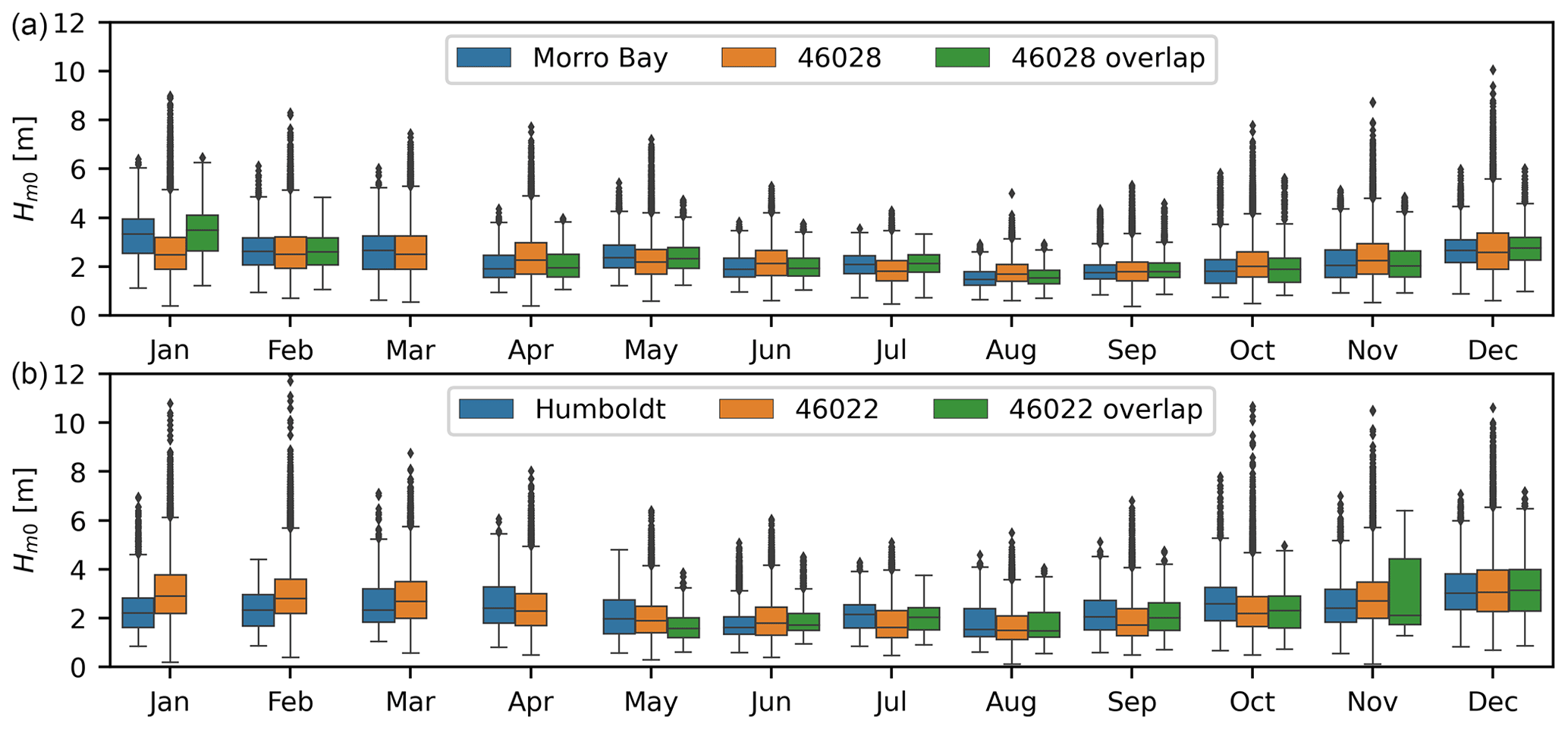
Figure 23 Monthly-average significant-wave-height distributions at (a) Morro Bay and (b) Humboldt. The buoys must have been active for at least 2 weeks for a month to be considered in the analysis. The median monthly significant wave heights are indicated with the horizontal lines within each box, the 25th and 75th percentiles form the colored box range, the whiskers are drawn at 1.5 times the interquartile range, and the dots are measurements outside of that range.

Waves near California are also seasonally variable in period and direction (e.g., Villas Bôas et al., 2017), and the lidar buoys measured these cycles at the WEAs (not shown for brevity). In addition, California experiences a multi-modal sea state where multiple sea states approach the coast simultaneously (Villas Bôas et al., 2017; Yang et al., 2020). The presence of multi-modal sea states in the WEAs complicate the description of the surface roughness. Model-based analysis of event prediction in the Mid-Atlantic Bight showed the effect that two-way coupled wave and atmospheric modeling has on accurate prediction of events (Gaudet et al., 2022). In that case, the atmospheric model obtained the surface roughness using the Taylor and Yelland (2001) parameterization with the wave model as input during runtime. Recent results suggest that using the mean wave period in surface roughness parameterizations can provide better results than the peak period (Sauvage et al., 2022). This dataset of colocated wind and wave measurements provides data for validation of these approaches. During the deployments, surface roughness estimates derived from the Taylor and Yelland (2001) parameterization for peak and mean wave periods show a difference of at least 1 order of magnitude. Figure 24 shows time series of surface roughness from October 2020 through to January 2021 at both buoys. The differences were consistent between the buoys.

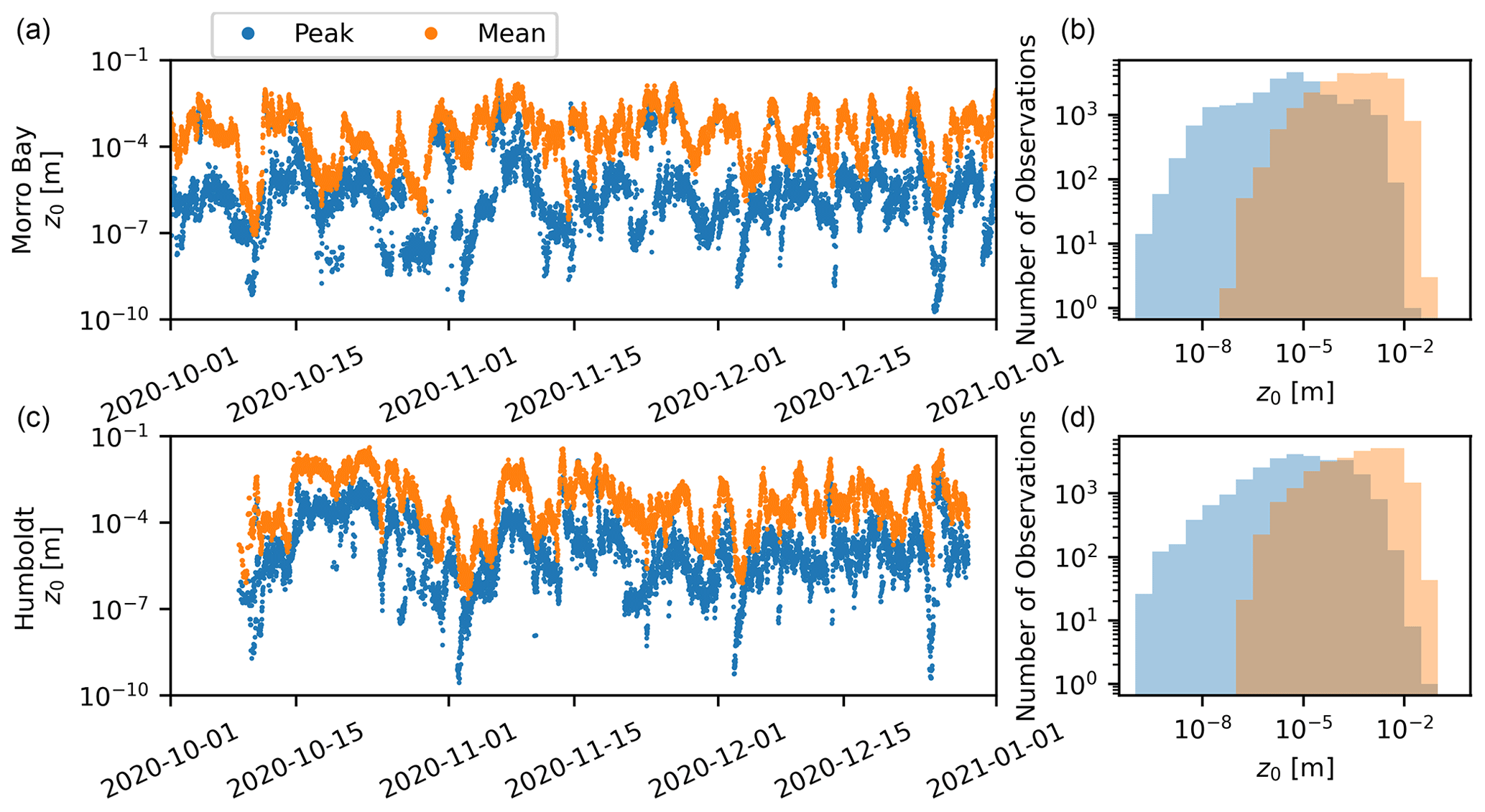
Figure 24 Surface roughness (a, b) at Morro Bay and (c, d) Humboldt. Peak and mean indicate surface roughness was calculated based on the peak wave period and mean wave period, respectively.

4.5 Cloud statistics

Clouds play a critical role in Earth's radiation balance. Atmospheric models have difficulty representing turbulent mixing processes within the boundary layer, which in turn affects the cloud representations in models. Therefore, studying the impact of clouds on boundary layer turbulence and vice versa is important to improve the accuracy of current-generation weather models. Figure 25 shows hourly cloud fraction estimates from the pyranometer data for the Morro Bay and Humboldt deployments. Both deployments show similar cloud distribution patterns, but the Morro Bay deployment shows a significantly higher density of clouds during the summer season compared to Humboldt. Additional analysis on the impact of turbulence due to the presence of clouds is a part of future work.

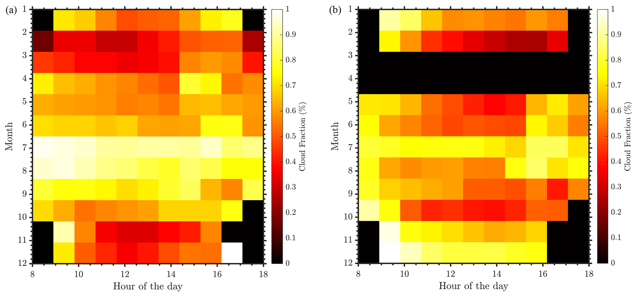
Figure 25 Cloud fraction estimates for Morro Bay (a) and Humboldt (b). A zero cloud fraction indicates no measurements during that time or data with poor quality.

4.6 Deviations from similarity theory

Theoretical wind profiles based on Monin–Obukhov (MO) similarity theory (MO) are often used in wind energy studies to extrapolate surface or near-hub-height measurements to hub height or above. During homogeneous and stationary atmospheric conditions, the non-dimensional wind shear (Φ_m), as per MO similarity theory, is a function of atmospheric stability and is given by Eq. (7)

$$\begin{array}{}\text{(7)}& {\mathrm{\Phi }}_{\mathrm{m}}\left(\mathit{\eta }\right)={\displaystyle \frac{kz}{u_{\ast }}}{\displaystyle \frac{\partial u}{\partial z}},\end{array}$$

where z is the height, u is the velocity, $\mathit{\eta }=z/L$ is the stability parameter, L is the Obukhov length (Monin and Obukhov, 1954), u_∗ is the friction velocity, and k is von Kármán's constant (0.4). The Obukhov length is a function of the friction velocity and buoyancy flux. Integrating Eq. (7) between z_o (surface roughness) and z (surface layer height) yields the well-known logarithmic wind profile equation.

$$\begin{array}{}\text{(8)}& \stackrel{\mathrm{‾}}{U}\left(z\right)={\displaystyle \frac{u_{\ast }}{k}}\left[\ln \left({\displaystyle \frac{z}{z_o}}\right)-{\mathrm{\Psi }}_{\mathrm{m}}\left({\displaystyle \frac{z}{L}}\right)\right],\end{array}$$

where Ψ_m accounts for the influence of stability on the wind profile (Monin and Obukhov, 1954). The Obukhov length (L) is given by

$$\begin{array}{}\text{(9)}& L=-{\displaystyle \frac{u_{\ast }^{\mathrm{3}}\stackrel{\mathrm{‾}}{{\mathit{\theta }}_{\mathrm{v}}}}{kg{\left(\stackrel{\mathrm{‾}}{w^{\prime }{{\mathit{\theta }}^{\prime }}_{\mathrm{v}}}\right)}_{\mathrm{s}}}},\end{array}$$

where θ_v is the virtual potential temperature, g is the gravitational constant, and ${\left(\stackrel{\mathrm{‾}}{w^{\prime }{{\mathit{\theta }}^{\prime }}_{\mathrm{v}}}\right)}_{\mathrm{s}}$ is the surface virtual potential temperature flux. When turbulent fluxes are not directly measured, they can be estimated from a bulk method when near-surface measurements of non-turbulent quantities are available (Fairall et al., 1996, 2003; Edson et al., 2013). The bulk method – the Coupled Ocean–Atmosphere Response Experiment (COARE) – relies on vertically integrated forms of MO similarity equations to relate interfacial differences of temperature, moisture, and wind components to their vertical turbulent fluxes. Necessary inputs include near-surface air temperature, relative humidity, wind speed, pressure (to compute air density), SST, significant wave height, and the phase speed of dominant waves. In general, the resultant bulk flux relations cannot be solved for the turbulent fluxes in closed form because the Obukhov length is itself a function of those fluxes. Thus, the bulk flux algorithm (except in idealized cases) becomes an iterative method to find a self-consistent set of turbulent fluxes for given non-turbulent inputs.

Deviations from MO theory within the marine boundary layer have been observed during stable atmospheric conditions (Vickers and Mahrt, 1999), low wind and fast swell cases (Grachev and Fairall, 2001), internal boundary layers (Vickers and Mahrt, 1999), and within the wave boundary layer (Davidson, 1974; Donelan et al., 1993; Smith et al., 1992). Most of these studies were conducted closer to the coast and observed larger wave-induced stresses, which affected the surface layer wind profile. In deep waters several kilometers away from the coast, the applicability of MO theory for non-dimensional wind shear estimates has still not been established in neutral and stable atmospheric conditions. In unstable atmospheric conditions, observations of wind shear follow conventional non-dimensional wind shear forms (Edson and Fairall, 1998; Edson et al., 2004), although the measurements were made at higher elevations compared to typical surface buoy heights. MO similarity theory is valid only within the surface layer, which is typically assumed to be equal to 10 % of the atmospheric boundary layer depth (h; Stull, 1998). Shallow marine atmospheric boundary layers can be observed offshore, which would significantly limit the application of similarity theory for wind energy applications. Figure 26 shows wind shear estimates measured between the surface anemometer and lidar measurements at 40 m as a function of atmospheric stability at the Morro Bay and Humboldt locations. The observed wind shear estimates were closer to the formulations from Beljaars and Holtslag (1991). Appendix A provides more details on the various similarity theory formulations used in Fig. 26.

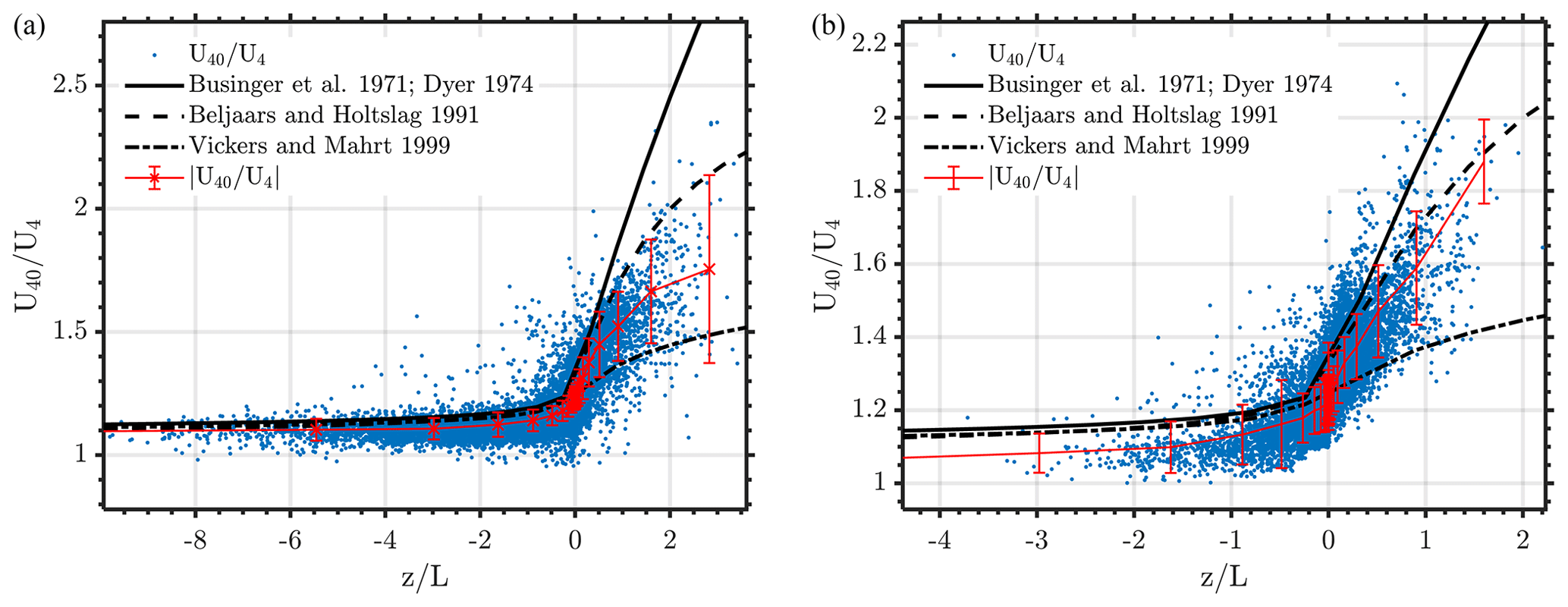
Figure 26 Wind shear observations at Morro Bay (a) and Humboldt (b) as a function of atmospheric stability. The blue dots represent 10 min observations of shear, the solid red line with crosses represents the bin-wise average, the solid black line represents the Businger–Dyer model wind shear estimate, the dashed black line represents the Beljaars and Holtslag model wind shear estimate, and the dash-dotted line represents the Vickers and Mahrt model wind shear estimate.

5 Code and data availability

All raw and post-processed data from this study are available on the Wind Data Hub website, https://a2e.energy.gov/data# (last access: 14 September 2023). The raw data (*.00) are used to create the final post-processed files (*.b0). Near-surface, wave, current, and cloud datasets for Humboldt are provided at https://a2e.energy.gov/ds/buoy/buoy.z05.b0 (last access: 14 September 2023) (DOI: https://doi.org/10.21947/1783807, Krishnamurthy and Sheridan, 2023b) and for Morro Bay at https://a2e.energy.gov/ds/buoy/buoy.z06.b0 (last access: 14 September 2023) (DOI: https://doi.org/10.21947/1959715, Krishnamurthy and Sheridan, 2023a). Lidar datasets for Humboldt are provided at https://a2e.energy.gov/ds/buoy/lidar.z05.b0 (last access: 14 September 2023) (DOI: https://doi.org/10.21947/1783809, Krishnamurthy and Sheridan, 2023d) and for Morro Bay at https://a2e.energy.gov/ds/buoy/lidar.z06.b0 (last access: 14 September 2023) (DOI: https://doi.org/10.21947/1959721, Krishnamurthy and Sheridan, 2023c). Additional codes to read the raw lidar data are available at https://github.com/rkpnnl/DOE_Buoy_DAP (last access: 1 December 2023; DOI: https://doi.org/10.5281/zenodo.10223643, Krishnamurthy, 2023). All post-processed data are available in standard NetCDF or *.csv format.

6 Conclusions

PNNL, in partnership with DOE and BOEM, deployed two buoys off the coast of California in autumn 2020 in areas targeted for offshore wind development. The buoys were outfitted with state-of-the-art instruments, including Doppler lidars, to further our understanding of atmospheric and oceanographic characteristics of the area and provide much needed data to inform the siting and leasing of offshore wind energy. Buoy measurements are valuable for studying basic science of offshore wind profiles, validating or calibrating atmospheric and oceanographic models, and developing new parameterization schemes. In this article, a summary of measurements, data-processing details, and results from lidar and other instruments aboard the buoys is presented. The final post-processed data are available to download on the Wind Data Hub.

All surface meteorological data were filtered and compared with nearby NDBC buoy measurements, with wind speed correlations of 0.98 at Morro Bay and 0.91 at Humboldt. In addition, the buoys provided a sense of the local atmospheric stability in the two regions – there was a higher likelihood of unstable atmospheric conditions at Morro Bay, while conditions were stable in the summer and unstable in the winter at Humboldt. Atmospheric models tend to deviate during stable atmospheric conditions, and such data are valuable for evaluating the accuracy of model simulations (Bodini et al., 2022). Novel analysis using buoy-based pyranometers was also conducted, which provided details about the cloud cover and aerosol optical depth over the regions. Along the US west coast, shallow marine boundary layers have been frequently observed (Beardsley et al., 1987; Burk and Thompson, 1996), which are generally encountered with clouds. Clouds are known to affect boundary layer turbulence, and a thorough understanding of how current-generation atmospheric models predict cloud patterns within the region is therefore important for future research. In addition, a thorough analysis of the wave sensor and ocean current data was performed, providing details of the multi-model sea state in the call areas about this essential characteristic for floating offshore wind farms. These data will also help support the development and validation of coupled ocean–wind–wave models (Gaudet et al., 2022).

In the Doppler lidar data, motion correction had a small impact on the 10 min wind speeds when compared to the uncorrected winds. At Humboldt and Morro Bay, negligible differences were observed between the uncorrected wind speeds and the corrected wind speeds. The STA wind speeds, on the other hand, were found to be about 4 % higher than the corrected wind speeds at Humboldt and about 3 % higher at Morro Bay. Differences between the corrected and uncorrected results were larger for second-order moments like variance or TI. At Humboldt, the uncorrected TI was on average about 0.6 % higher than the corrected result. For Morro Bay, the uncorrected TI was about 0.4 % higher than the corrected result. By contrast, STA TIs are significantly higher than either the corrected or uncorrected results. STA TIs were on average 54 % higher than the corrected variances at Humboldt and 55 % higher at Morro Bay. Motion correction also impacted estimates of vertical velocity. At Humboldt, the uncorrected vertical velocity was 68 % higher compared to the corrected result. For Morro Bay, the uncorrected vertical velocity was 28 % higher than the corrected result. By contrast, STA vertical variances were 172 % larger than the corrected variances at Humboldt and 124 % larger at Morro Bay. For turbulence estimates, the net effect of motion correction is primarily to reduce the horizontal and vertical velocity variances. The STA results presented here were obtained using erroneous pitch and roll information from the WindCube's internal IMU. As a result, the STA results contain unrealistically large estimates of velocity variance that in turn result in unrealistically large estimates of turbulence kinetic energy and TI.

Over the last few decades, logarithmic wind profiles have been used extensively in the wind energy resource assessment studies (e.g., Holtslag, 1984; Emeis, 2010, 2014; Drechsel et al., 2012; Krishnamurthy et al., 2013). In particular, the logarithmic wind profile model has been used to extrapolate observed wind speeds to hub height (e.g., tower measurements), interpolate winds between two atmospheric model levels (Sheridan et al., 2020), and extrapolate geostrophic winds to hub height using the friction velocity computed from the geostrophic-drag law (Tennekes, 1973). Because these models typically break down above the surface layer, such models must be used with caution during shallow marine boundary layers. Using the lidar data collected over an annual cycle, it was observed that the similarity theory model developed by Beljaars and Holtslag (Beljaars and Holtslag, 1991) compared well with observations. Other models tend to either overestimate or underestimate the shear within the region.

The analyses contained in this article provide significant new information about the offshore conditions along the US west coast. In addition, the experience gained will inform both configurations and analysis of the data from future deployments of these lidar buoy systems.

Appendix A: Monin–Obukhov similarity theory

Three prominent similarity-theory-based models are generally used in atmospheric studies – the Businger–Dyer (BD; Businger et al., 1971; Dyer, 1974), Beljaars and Holtslag (BH; Beljaars and Holtslag, 1991), and Vickers and Mahrt (VM; Vickers and Mahrt, 1999) models. For reference, their stability functions are given here. The BD functions for stable (η≥0) and unstable atmospheric (η<0) conditions are given by

$$\begin{array}{}\text{(A1)}& {\mathit{\psi }}_{\mathrm{BD}}\left(\mathit{\eta }\right)=\left\{\begin{array}{l}-\mathrm{6}\mathit{\eta },\text{for}\mathit{\eta }\ge \mathrm{0};\\ \mathrm{2}\log \left(\frac{\mathrm{1}+x}{\mathrm{2}}\right)+\log \frac{\mathrm{1}+x^{\mathrm{2}}}{\mathrm{2}}-\mathrm{2}\mathrm{atan}\left(x\right)+\frac{\mathit{\pi }}{\mathrm{2}},\\ \text{for}\mathit{\eta }<\mathrm{0};\end{array}\right.\end{array}$$

where $x={\left(\mathrm{1}-\mathrm{19.3}\mathit{\eta }\right)}^{\mathrm{1}/\mathrm{4}}$. Similarly, the BH stability functions are given by

$$\begin{array}{}\text{(A2)}& {\mathit{\psi }}_{\mathrm{BH}}\left(\mathit{\eta }\right)=\left\{\begin{array}{l}-a\mathit{\eta }-b(\mathit{\eta }-\left(\frac{c}{d}\right))\exp (-d\mathit{\eta })-bc/d,\\ \text{for}\mathit{\eta }\ge \mathrm{0};\\ \frac{\mathrm{3}}{\mathrm{2}}\log \left(\frac{\mathrm{1}+x+x^{\mathrm{2}}}{\mathrm{3}}\right)-\sqrt{\mathrm{3}}\mathrm{atan}\left(\frac{\mathrm{2}x+\mathrm{1}}{\sqrt{\mathrm{3}}}\right)+\frac{\mathit{\pi }}{\sqrt{\mathrm{3}}},\\ \mathrm{for}\mathit{\eta }<\mathrm{0};\end{array}\right.\end{array}$$

with a=1, $b=\mathrm{2}/\mathrm{3}$, c=5, d=0.35, and $x={\left(\mathrm{1}-\mathrm{12.87}\mathit{\eta }\right)}^{\mathrm{1}/\mathrm{3}}$. The VM stability functions are given by

$$\begin{array}{}\text{(A3)}& {\mathit{\psi }}_{\mathrm{VM}}\left(\mathit{\eta }\right)=\left\{\begin{array}{l}-\mathrm{3}x+\log \mathit{\eta }-\log \left(\mathrm{1}-x\right)+\frac{\mathrm{1}}{\mathrm{2}}\log \left(x^{\mathrm{2}}+x+\mathrm{1}\right)\\ +\sqrt{\mathrm{3}}\mathrm{atan}\left(\frac{\mathrm{2}x+\mathrm{1}}{\sqrt{\mathrm{3}}}\right),\text{for}\mathit{\eta }\ge \mathrm{0};\\ \mathrm{2}\log \left(\frac{\mathrm{1}+y}{\mathrm{2}}\right)+\log \left(\frac{\mathrm{1}+y^{\mathrm{2}}}{\mathrm{2}}\right)-\mathrm{2}\mathrm{atan}\left(y\right)+\frac{\mathit{\pi }}{\mathrm{2}},\\ \text{for}\mathit{\eta }<\mathrm{0};\end{array}\right.\end{array}$$

where $x={\left(\mathrm{1}+\mathrm{16}\mathit{\eta }\right)}^{\mathrm{1}/\mathrm{3}}$, and $y={\left(\mathrm{1}-\mathrm{35}\mathit{\eta }\right)}^{\mathrm{1}/\mathrm{4}}$.

Appendix B: Data files, naming convention, and list of instruments

Data collected from past and current buoy deployments are made available for public access within the DAP (https://a2e.energy.gov/data, last access: 14 September 2023). All processed data are uploaded after complete datasets are recovered from the buoy during schedule maintenance visits and after buoy recovery. Data available from the buoy processed data files include the measurements described in Table B1. All times are in UTC.

The file naming convention used for the data files is given below:

• “AAAA.z##.b0.yyyymmdd.hhmmss.BBB.a2e.ccc”,

  where

  • AAA is data source, e.g.,

    • “buoy”

    • “lidar”

  • ## is the buoy deployment number, e.g.,

    • “05” for the Humboldt deployment,

    • “06” for the Morro Bay deployment;

  • yyyymmdd is the calendar date when the data file begins;

  • HHMMSS is the time, in UTC, when the data file begins;

  • BBB is the measurement type (“currents”, “waves”, “lidar”, etc.); and

  • ccc is the filetype, e.g.,

    • “.csv”

    • “.nc”

Table B1 Description of measurements, variables, and units.

Appendix C: IMU buoy swing test results

Figure C1 shows sample data from the buoy swing test at Humboldt prior to the deployment. All IMUs were calibrated during the swing test and showed consistent results, although the WindCube IMU consistent performed poorly during the deployment, which is also shown in Sect. 3.2.

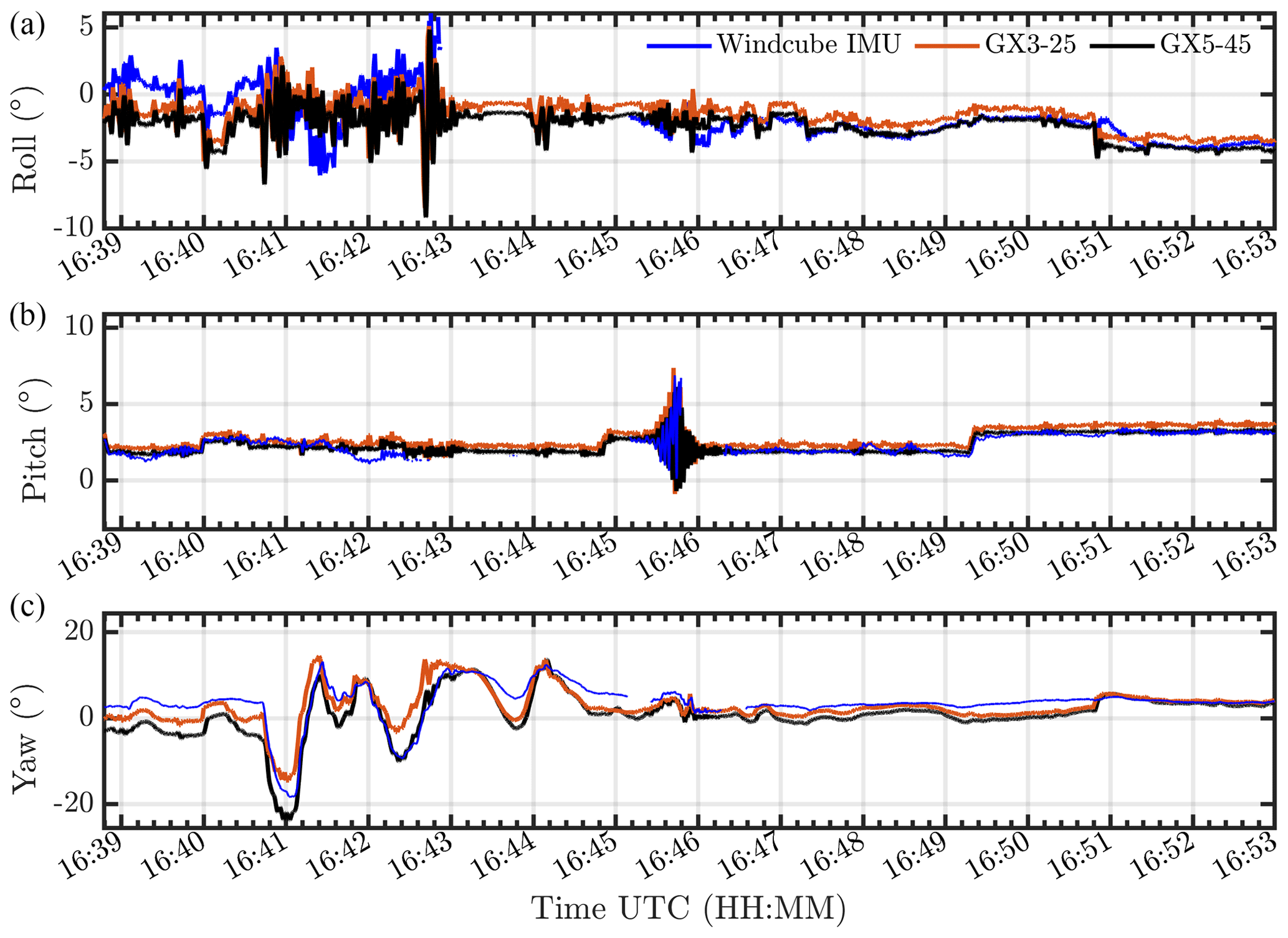
Figure C1 Buoy swing test results showing the IMU data from the WindCube, GX3-25, and GX5-45 at Humboldt.