The use of GRDC gauging stations for calibrating large-scale hydrological models

The Global Runoff Data Centre (GRDC) provides time series of observed discharges and information on hydrometric stations that are valuable for calibrating and validating the results of hydrological models. We address a common issue in large-scale hydrology that has not been satisfactorily solved, though investigated several times. To compare simulated and observed discharge, grid-based hydrological models must fit reported station locations to the resolution-dependent gridded river network. We introduce an intersection-over-union ratio approach to selected station locations on a coarser grid scale, reducing the errors in assigning stations to the correct upstream basin. We update the 10-year-old database of watershed boundaries with additional stations based on a high-resolution (3 arcsec) river network and provide source codes and high- and low-resolution watershed boundaries to easily select stations for calibration/validation of hydrological models. The dataset is stored on Zenodo with the associated DOI: https://doi.org/10.5281/zenodo.6906577 (Burek and Smilovic, 2022).

1 Introduction

River discharge is one of the most important variables in hydrological modeling because all basin processes are integrated into this variable. Discharge spatially and temporally integrates the range of meteorological variables and basin characteristics. Spatially and temporally distributed properties of river and lake morphology, soil, groundwater, snow, glaciers, climate, land cover, and human interaction influence discharge at the outlet of a basin. Discharge is extremely useful for calibrating and validating global hydrological models (Müller Schmied et al., 2021; Sutanudjaja et al., 2014; Hanasaki et al., 2008) using different objective functions, such as Nash–Sutcliffe (Nash and Sutcliffe, 1970) and Kling–Gupta (Kling et al., 2012). It is also useful for tasks like estimating flood hazards (Alfieri et al., 2015), inland navigation (Nilson et al., 2012; Christodoulou et al., 2020), energy power production (Hunt et al., 2020; Van Vliet et al., 2016), and water scarcity (Hoekstra et al., 2012; Van Beek et al., 2011).

Since the establishment of the Global Runoff Data Centre (GRDC) database (Vorosmarty et al., 1998; Fekete et al., 2002), the number of stations has increased and the number of publications using the GRDC dataset has also grown – the GRDC publication database of 2021 (GRDC, 2020) references 118 publications using the discharge time series. The Generic Statistical Information Model (GSIM) database (Do et al., 2018) provides a good overview of several river discharge databases worldwide. Although there are several public databases of river discharge at a basin scale (e.g., Mekong Basin, Mekong River Commission, 2023), the GRDC database offers the richest source of global river discharge data, as follows.

A global hydrological database is essential for research and application-oriented hydrological and climatological studies at global, regional, and basin scales. The Global Runoff Database is a unique collection of river discharge data on a global scale. It contains time series of daily and monthly river discharge data of well over 10 000 stations worldwide. This adds up to around 470,000 station years with an average record length of 45 years (GRDC, 2020).

The GRDC database of river discharge comes with information about the stations from the data providers, like the location of the station, name of the station and the river, upstream area, elevation, mean discharge, and more. The location and the upstream area are especially important in comparing model results from hydrological models with station discharge data.

Quality checking of station attributes and spatial redistribution of station locations for different gridded river networks for hydrological models have been carried out since the beginning of GRDC data collection (Fekete and Vörösmarty, 1999) and for each model repeatedly (Sutanudjaja et al., 2018; Zhao et al., 2017; Wang et al., 2018). For example, to test the Community Water Model (CWatM) (Burek et al., 2020) global model performance at 30 arcmin (=0.5^∘ ≈50 × 50 km; hereafter, 30^′) resolution, we used the station data and the global drainage direction map (DDM30) network (Döll and Lehner, 2002) and corrected the locations to fit with the approach of Zhao et al. (2017). Several errors can occur when the discharge station is used for gridded hydrological modeling, as follows.

1. The station location is not at the correct location and is too far from the river.

2. The station location is at the correct location, but because of the river width and/or the grid resolution of a high-resolution river network, the station location is not in the appropriate grid cell of the river network or because, even at 100 m, the network is not high-resolution enough to capture the station location.

3. The high-resolution network does not represent reality (e.g., the river does not flow in the deepest part of the valley because of human interventions).

4. Upscaling error: when a coarser resolution for hydrological modeling is applied (e.g., 30^′), using the original station location might lead to its position being wrongly assigned because, for instance, the coarser grid cell river network may include the junction with a tributary. In contrast, the station may indicate the tributary itself.

5. Mismatch error: suppose the station location is selected only by comparing the upstream area of the upscaled network with the reported upstream area. In this case, a station could be assigned to the wrong basin because the upstream area fits slightly better.

6. The global station density is unevenly distributed. We find a high density for North America and Europe and a low density for Asia and Africa. In North America and Europe, some stations are close downstream to other ones, even though no significant tributaries are entering.

This paper aims to provide a Python code to easily select stations for calibration/validation of hydrological models by addressing these possible errors and giving examples of how to correct them. Lehner (2012) calculated explicit watershed boundaries for 7163 basins on a high-resolution network. These watershed boundaries are freely available on the GRDC website (GRDC, 2020). We repeated this exercise but using a higher-resolution network based on a more up-to-date dataset, the 3 arcsec (∼100 m or exactly 92.61 m at the Equator, hereafter, 3^′′) MERIT hydro-network (Yamazaki et al., 2019) rather than the 15 arcsec (∼500 m) HydroSHEDS (Lehner et al., 2008). Moreover, we used a greater number of GRDC stations, including those added in the last 10 years (10 701 stations as opposed to 7532). In addition to the high-resolution basins, we added a method for upscaling each station automatically to 5^′ (∼10 km) and 30^′ (∼50 km) using a more advanced method than simply comparing the river network upstream area with the reported upstream area. Using this method, a selection of stations can be appropriated to the resolution of the hydrological model. Furthermore, our code is available and open source in Python to change or calculate stations for individual applications.

2 Methods

The methods can be split up into three main groups, each group building upon the results of the previous one. The first method describes allocating a station location from the GRDC database to fit best on a high-resolution network. This method reproduces the approach from Lehner (2012). The second method describes how to upscale the station location from a high-resolution network to a low-resolution network used in standard land surface hydrological routing models by comparing upstream areas and the similarity of the station upstream areas at high and low resolution. The third method describes how to select the most appropriate stations for calibrating hydrological models, depending on the metadata of the stations and the chosen model grid resolution.

2.1 Procedure for station allocation on a high-resolution network

2.1.1 Automatic procedure

We used the MERIT hydro database of Yamazaki et al. (2019), which comes as an open-source database in chunks of 5^∘ × 5^∘ at 3^′′ resolution (36 billion grid cells per 5^∘ × 5^∘). We used the river network direction maps and applied the D8 flow model convention: either each grid cell can flow into one of the eight neighboring grid cells or it is a sink. This approach, which does not allow rivers to be split into two streams or grid cells to contribute to several basins simultaneously, is used in most land surface models and grid-based hydrological models. We obtained the upstream area of each high-resolution grid cell from the upstream area in square kilometers from the MERIT dataset. For the evaluation, we used all stations with a reported upstream area greater than or equal to 10 km² (124 stations have an upstream area smaller than 10 km²) or with no reported upstream area record (327 have no upstream area record in the GRDC dataset).

For the automatic station allocation, we mainly follow the protocol of Lehner (2012) as follows.

1. A rectangular search radius of 165 arcsec (∼5 km) for each station was defined.

2. For each grid in this rectangle, the upstream drainage area (UPA) from the network from Yamazaki et al. (2019) was compared to the area reported in the GRDC, and the upstream area accordance is computed as follows:

   upstream area accordance = GRDC reported UPA $/$ gridded network UPA (where GRDC reported UPA < gridded network UPA);

   upstream area accordance = gridded network UPA $/$ GRDC reported UPA (where GRDC reported UPA ≥ gridded network UPA).

3. All cells with an upstream area accordance of less than 50 % were dismissed from further evaluation.

4. A first ranking scheme – area discrepancy (RA) – was calculated with values between 0 (best fit) and 50:

   RA = 100 – upstream area accordance [%].

5. For the second ranking scheme – distance (RD) – the distance of the cell to the reported station location in the GRDC database was calculated and normalized to obtain the value 0 at the station location and 50 in 5 km distance.

6. An objective criterion (OC) for ranking was computed by OC = RA + 2 ⋅ RD. The equation and weighting were taken from Lehner (2012).

7. The grid cell with the lowest OC value was taken as the corresponding grid cell for the station location on a high-resolution network.

8. If no station location was found in this step, the search radius was increased to 5^′ (∼10 km), OC was calculated as OC = RA + RD, and the lowest OC value was taken as the corresponding grid cell.

2.1.2 Manual procedure for the remaining stations

For the ∼7.5 % of the stations that failed both rounds of searching, we carried out the following manual inspections.

• For the 3 % of stations in the GRDC database (327 stations) with a reported area of −999, we used the next biggest river. We checked manually with GIS, but we did not check all station information manually (e.g., station name, river name, and altitude).

• For the 1.5 % of stations that failed the automatic search but had a valid UPA record (169 stations), we manually checked and assigned a location in the range of up to 120 km from the original site (to address any typographical error, e.g., 51.57^∘ instead of 52.57^∘).

• For the 2.2 % of the stations (228 stations), we could not find an adequate location on the high-resolution network – perhaps due to errors in the GRDC database or insufficient network maps (e.g., missing canals, braided rivers, diversion, and confluent rivers)

2.1.3 Output: polygons of basins

For 10 349 basins, we assigned polygons based on the reallocated station locations at high resolution (3^′′) with the Python library flwdir from Eilander et al. (2021) and the river direction mosaic maps from Yamazaki et al. (2019). Like the original from Lehner (2012), we produced two versions: (a) polygons that follow the exact grid cell contours with high memory requirements and (b) a version with smoothed edges and low memory consumption. The resulting shapefiles were produced in the ESRI shapefile format and included the station information from GRDC. This process addresses errors (1), (2), and (3) (noted above) and provides an update to the shapefiles of Lehner (2012).

2.2 Upscaling station location to a coarser grid cell resolution

The main idea of creating a new set of high-resolution watershed boundaries is not only to update the work of Lehner (2012) but also to use a different method of assigning station discharge time series to the correct grid cell in grid-based hydrological models. Global hydrological models use 30^′ resolution in the ISIMIP3 project (Warszawski et al., 2014). The trend for global modeling is to move toward higher resolutions at 5^′ and hyper resolution (≤1 km) (Bierkens, 2015). For regional studies (Hanasaki et al., 2022; Guillaumot et al., 2022), the resolution is already 1 km or below. Approaches to upscaling to coarser resolutions are mainly based on comparing the reported UPA and the UPA calculated from the river network (Fekete and Vörösmarty, 1999; Zhao et al., 2017).

With the flwdir tool from Eilander et al. (2021) and with the idea of Munier and Decharme (2022) of comparing the similarity of shapes, it is possible to introduce another objective criterion – the similarity of high-resolution watershed boundaries and low-resolution boundaries. Using the method of comparing upstream areas, we can partly address error (4) upscaling error but not errors (5) and (6).

For an automatic upscaling process, we used the following protocol.

• We defined a minimum UPA for the station we wanted to use in the low-resolution hydrological model (e.g., UPA ≥ 9000 km² for 30^′ (∼3 cells), UPA ≥ 1000 km² for 5^′ (∼12 cells)).

• To find the grid cell on the coarse-resolution network which best fits the UPA and the shape of the high-resolution network, we calculated two objective criteria for all coarse grid cells with a distance ≤2 coarse cell distance (altogether 25 grid cells) to the location of the station on the high-resolution network (see Fig. 1)

• For each coarse grid cell, the coarse UPA was derived, and the upstream area accordance was computed as first objective criterion:

  upstream area accordance = GRDC reported UPA $/$ coarse UPA (GRDC reported UPA < coarse UPA);

  upstream area accordance = coarse UPA $/$ GRDC reported UPA (GRDC reported UPA ≥ coarse UPA).

• The upstream area accordance can have a value of [0,1], where a value of 1 means that GRDC and coarse UPA have the same upstream area.

• The second objective criterion was the intersection-over-union ratio (Rezatofighi et al., 2019; Munier and Decharme, 2022): intersection-over-union ratio = area of intersection $/$ area of union.

  Therefore the watershed shape for the station at high resolution is created and compared to the watershed shape for the station at low resolution. The area of intersection represents the area that the high-resolution shape and the low-resolution shape have in common. The area of union represents the area of the combined shapes of high and low resolution. The intersection-over-union ratio can have a value of [0,1]. The closer to 1 the intersection-over-union ratio value, the more similar the shapes are.

• To reduce the two objective criteria to one solution, the minimum Euclidian distance between the best possible solution (at 0,0) and the two objective criteria was calculated. Both objective criteria have a range of [0,1]. Therefore, we decided to use a weighting factor of 1 for both criteria.

  $$\mathrm{\text{ED}}=\sqrt{{\left(\mathrm{1}-\text{upstream area accordance}\right)}^{\mathrm{2}}+{\left(\mathrm{1}-\text{intersection-over-union ratio}\right)}^{\mathrm{2}}}$$

• The low-resolution coordinates with minimum Euclidian distance were chosen as the station coordinates for this grid size resolution.

Figure 1 illustrates this method for low resolution (5^′) and for cell location No. 7, which is one 5^′ cell south of the cell where the Passau/Inn station is located (see the enlarged inset in the top left of Fig. 1). Even if this cell does not represent the cell where the station is located, it fits the upstream area accordance and the best intersection-over-union ratio of all 25 cells around the station location.

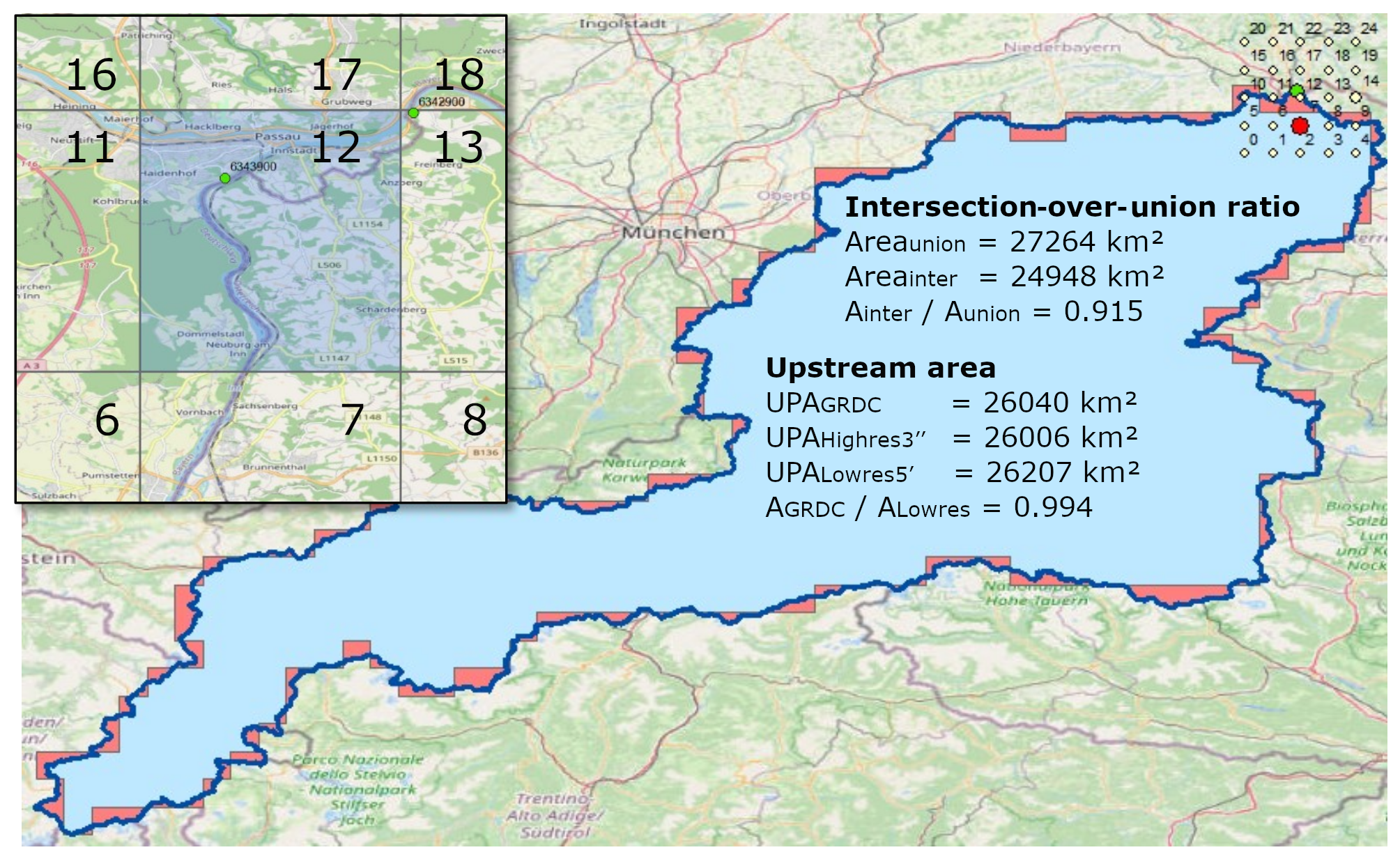
Figure 1 Intersection-over-union ratio for the River Inn basin in Passau, Germany, GRDC 6343900. The dark blue line is the watershed of the Inn up to Passau at high resolution (3^′′). The light blue is the intersection between the low-resolution Inn at 5^′ and 3^′′, and red signifies the union of the 5^′ basin with the 3^′′ basin. © OpenStreetMap contributors 2022. Distributed under the Open Data Commons Open Database License (ODbL) v1.0.

Figure 2 shows four examples of the 25 cell locations around the Passau/Inn station. Figure 2a uses the cell where the station is located. This cell represents not only the Inn but the also the Danube and the Inn Basin. Figure 2b includes only a small tributary of the Inn and Fig. 2c contains only the Danube Basin but not the Inn Basin. Figure 2d shows the best location (one grid cell south of the grid cell with the station – same as in Fig. 1).

As a result, we obtain a pair of coordinates for each station at a coarser resolution. Here we chose 5^′ and 30^′. For 5^′, the network from Eilander et al. (2021) was used based on the high-resolution network from Yamazaki et al. (2019), while for 30^′, the DDM30 network from Döll and Lehner (2002) was used, as this is the agreed upon network for the ISIMIP2 and ISIMIP3 (Frieler et al., 2017) hydrological modeling efforts.

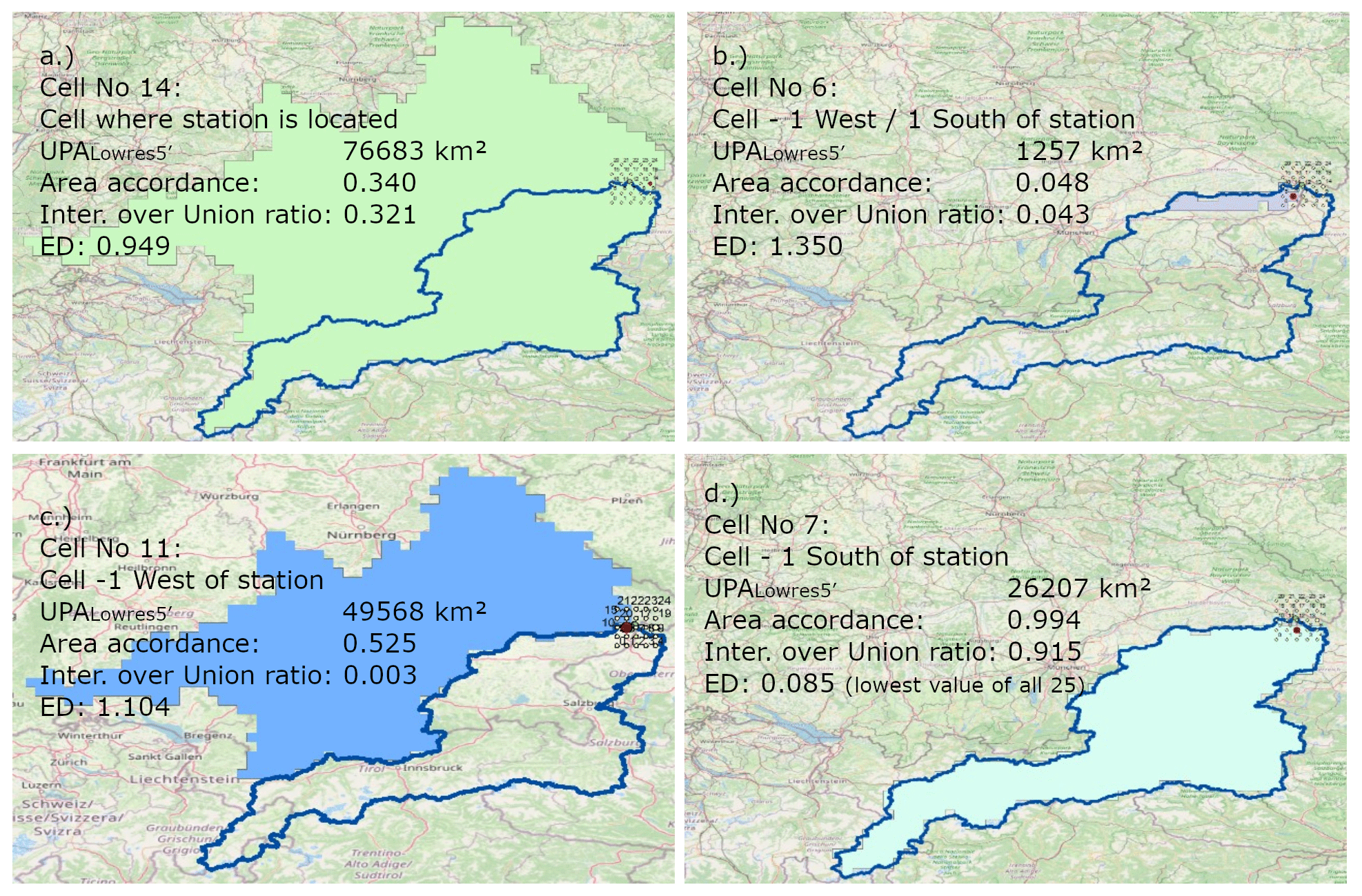
Figure 2 Concept of similarity for the Passau/Inn station, Germany – GRDC 6343900 with a high-resolution watershed map shown in blue outline and four different watershed maps based on a 5^′ resolution network around the station location. © OpenStreetMap contributors 2022. Distributed under the Open Data Commons Open Database License (ODbL) v1.0.

2.3 Selecting station for calibration of a hydrological model based on metadata

In the previous step, we selected stations based solely on location metadata. For the next selection step, we included meta information of time series like length, end date, and the number of missing values in a time series. For calibration or validation, the unsuitable stations were those with only short time series, those that ended too far in the past, and those with too many missing values. The criteria for “too short” and “too old” are subjective and can be chosen in another way, as in Alfieri et al. (2020), but if the criteria are not strong enough, post-selection can be done. If they are too rigid, the settings part of the Python code can be changed. Fortunately, all the necessary information is included in the metadata file from GRDC.

2.3.1 Deselection and ranking criteria

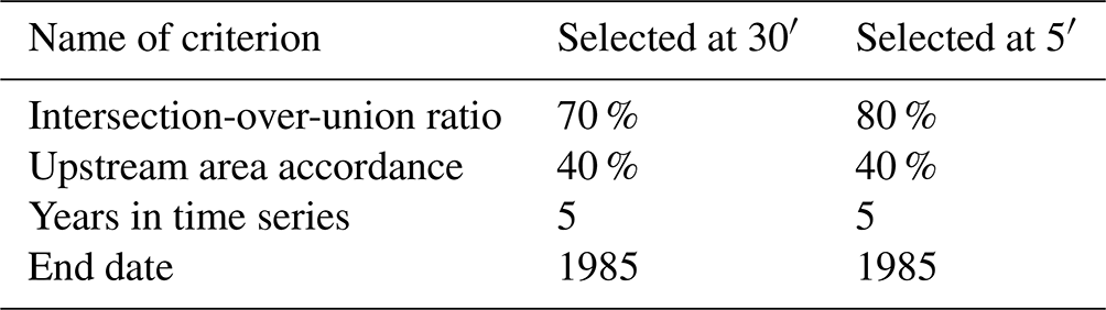
We included several criteria for selecting or deselecting a station (see Table 1). We derived the first two criteria from the previous analysis of the station location.

• The accordance of the UPA on the chosen resolution with the area reported from GRDC: here, we chose a relatively forgiving upstream area accordance. If the upstream area of the selected resolution had a criterion of more than 40 %, this criterion is fulfilled. In most cases, the area was above this ratio, but we did not want to deselect stations where the GRDC record might be accurate.

• The intersection-over-union ratio between the high-resolution shapefiles and the shapefile of the chosen resolution.

We included two selection criteria from the metadata information about the time series.

• The time series should have at least 5 years of monthly or daily records.

• The end date of a time series should be later than 1985.

Table 1 Selection criteria based on low resolution.

2.3.2 Division of stations

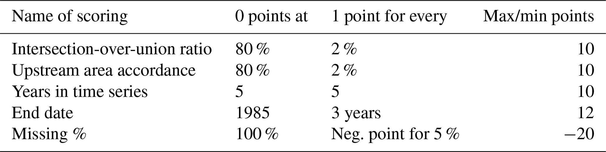
The stations may be too close to each other for it to be worth calibrating both. We checked the similarity of the low-resolution shapefiles. If they were equal to or more than 95 % similar, we decided to calibrate only one station and keep the other for validation purposes. To choose which of the similar stations we kept for calibration, we introduced a ranking/scoring system.

If a station had a higher intersection-over-union ratio or upstream area accordance than 80 %, it received one scoring point for every 2 %. Stations earn scoring points for every 5 additional years of time series length and for time series end dates after 1985. For missing data in the time series, scoring points are subtracted (see Table 2 for the scoring criteria). The station with the higher score is chosen. These criteria are subjective and can be changed in the Python code.

Table 2 Scoring where two stations are too similar.

2.3.3 Output: list of stations to be appropriated for calibration

As a result of this step, we obtained two tables for 30^′ and 5^′ that distinguished the stations as useful for calibration, as useful for validation, and as not recommended for calibration or validation. All evaluation was solely based on the metadata file provided by GRDC.

3 Results

3.1 Station allocation at high resolution

The March 2022 GRDC station dataset has 10 701 stations in total. We used only those stations with a UPA equal to 10 km² (thus discounting 124 stations), but we kept the stations without data for the UPA (327 stations). We used an automatic detection method to find the best location for each station on the high-resolution MERIT network at 3^′′. In addition we did a manual search for 169 stations, but we still had 228 stations which we could not assign to a basin. Figure 3 shows the global distribution of GRDC stations (status as of March 2022), with a high concentration of stations in North America and Europe and a lower and more clustered distribution in Africa and Asia.

For further analysis, we had 10 349 stations with a counterpart in a location on the MERIT network and an assigned basin at 3^′′ resolution, and 49 of these basins did not have a reported area in GRDC. From the remaining 10 300 stations, we calculated the area in accordance with the GRDC reported UPA and the area calculated on the high-resolution network using UPA maps from Yamazaki et al. (2019). We kept only those with an upstream area accordance ≥0.4 (10241 stations). For hydrological modeling, this accordance might be too low. Still, we assumed there were some errors in the reported area of GRDC and that these stations could be deselected in a further step, if necessary.

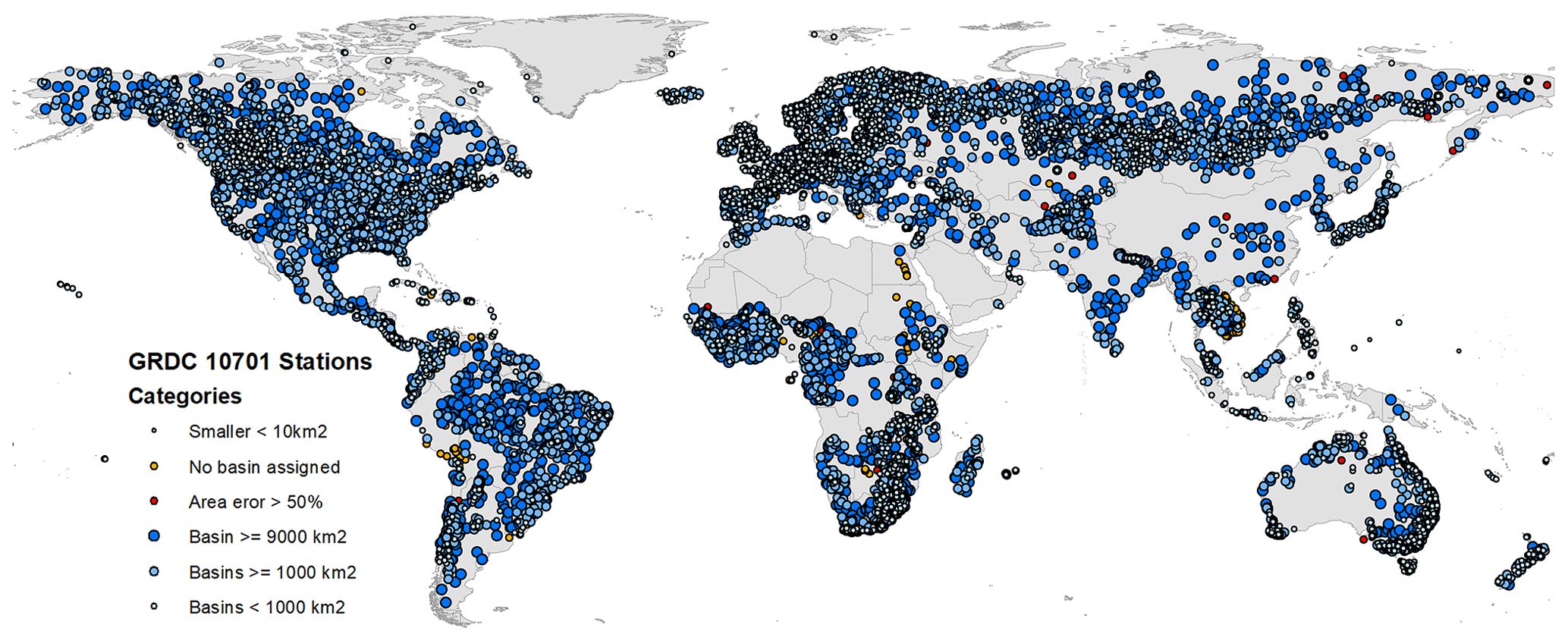
Figure 3 Location and categories of 10 701 GRDC stations (world administrative boundaries by https://www.opendatasoft.com, last access: 6 December 2023).

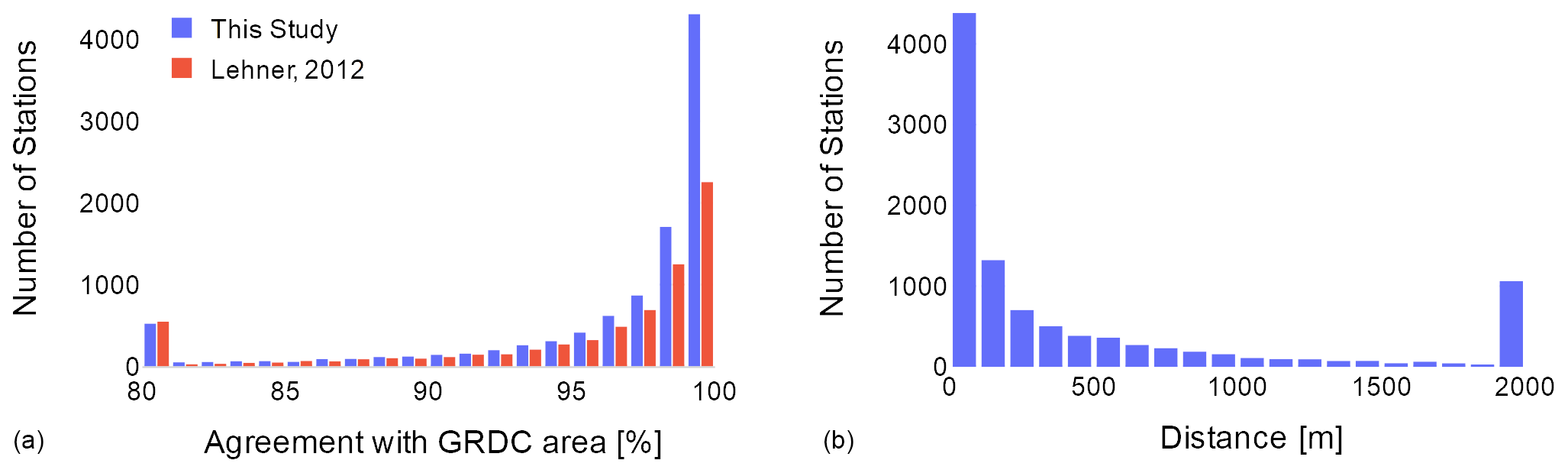
Figure 4 Histogram of (a) accordance with GRDC upstream area and (b) distance from the corrected location to the GRDC location.

The histogram of upstream area accordance in Fig. 4a and Table 1 shows that a high number of stations (43 %) have upstream area accordance that is equal to or more than 99 % (an area error of less than 1 %). Compared with the work of Lehner (2012), we obtained a slightly higher percentage of accordance in this class but with almost twice as many stations (4332 vs. 2422). Here, 88 % (85 % for Lehner, 2012) still had good accordance of 90 % or more. There were 330 stations with an area accordance of less than 75 %, 18 stations with less than 50 %, while 49 stations had no area reported.

Figure 4b shows the distance in meters from the reported station coordinates in GRDC and the station location according to the high-resolution network. A necessary shift in stations might be required because (a) the river network is not high resolution enough to capture the river (see Fig. 5d) or (b) the river width is greater than 90 m, and it would be necessary to shift the station location from the river shore into the middle of the river to match the high-resolution network. However, we assumed that most distance errors greater than 500 m come from the stations being wrongly allocated. Table 3 shows that the percentage of upstream area accordance negatively correlates with the distance median. Here, the distance is the distance in meters between the reported station location in the GRDC dataset and the location represented in the 3^′′ MERRIT network. The median distance is calculated as the median of distances for all stations in each row of Table 3.

Table 3 Comparison of stations with accordance in area of high-resolution basins with area reported from GRDC.

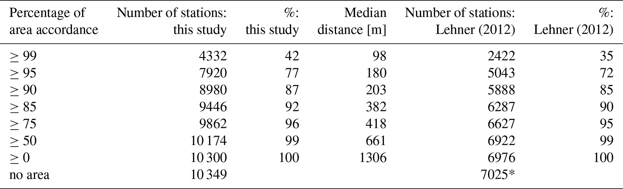
* Of 7163 stations in Lehner (2012), 7025 match the new dataset.

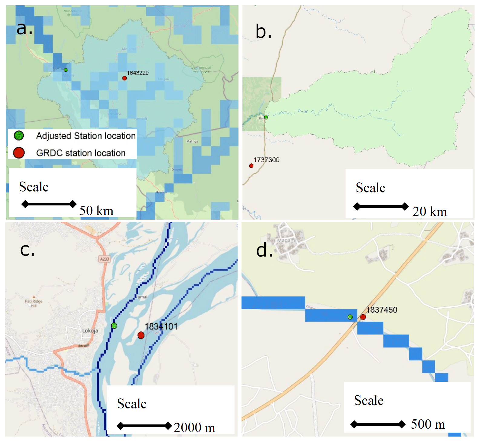
Figure 5 Possible errors in station location. © OpenStreetMap contributors 2022. Distributed under the Open Data Commons Open Database License (ODbL) v1.0.

Figure 5 shows some of the possible errors as well as the need to correct the station location that will be used in hydrological models as follows.

Part (a): GRDC station 1643220 Mouila-Val-Marie, Ghana, has a reported UPA of 15 900 km². The closest river to the station location has a high-resolution UPA of 2477 km². The next location with a closer upstream area to the reported one (15 868 km²) is 50 km to the west. Thus, here, either the station location or the reported area is wrong.

Part (b): GRDC station 1737300 Bamingui, Central African Republic, with a reported area of 4380 km², has no river of this size at a closer distance. We thus chose the river near the city of Bamingui with a high-resolution UPA of 6075 km² at a distance of 25.7 km from the GRDC station location.

Part (c) shows the station location of GRDC 1834101 Lokoja, Nigeria. The station seems to be on the Benue River, a tributary of the Niger River. According to Udo et al. (2021), the station is located on the Niger River, upstream of the junction of the Niger and Benue. Lehner (2012) assumed the station is downstream of the junction. No area is reported as being associated with this station, but the area could be 337 000 km² (Benue), 1 651 000 km² (upstream Niger), or 1 990 000 km² (downstream Niger).

Part (d) shows the GRDC station 1837450 at Challawa Bridge in Nigeria at the exact location underneath a bridge over the River Challawa. However, the high-resolution network of 90 m shows no river on this grid cell, and the station location must thus be shifted 90 m to the west.

Another example is GRDC stations 1396200, 1396201, and 1396210, which have the same reported location but different river station names and UPAs.

For GRDC station 4208919 on the Dunkirk River, Canada, we found a typographical error. Instead of 58^∘ N, it should be 56^∘ N.

Station Siramakana, Mali, at the Baoulé River GRDC station 1112330 is, according to Hydroscience Montpellier (2022), around 50 km from the station location mentioned in the GRDC dataset.

The remaining 10 241 stations are not equally distributed globally. There are regions where water cannot be measured as streamflow, such as Greenland, the Sahara, the Arab Peninsula, the Kalahari, and central Australia. In other regions, we know that streamflow is measured, but GRDC does not have the records (some parts of Italy, Indonesia); in some regions, we do not even know if there are measurements (e.g., North Korea). Some basins, especially in North America and Europe, have a dense reported discharge station network (e.g., the Danube). Figure 6 shows the number of subbasins of GRDC stations placed inside another station. For example, in the Danube, there is a station for the upper River Inn, which is inside the basin of the lower Inn (another station), which is inside the basin of the upper Danube, which is inside the basin of the middle Danube, just like the concept of Matryoshka dolls.

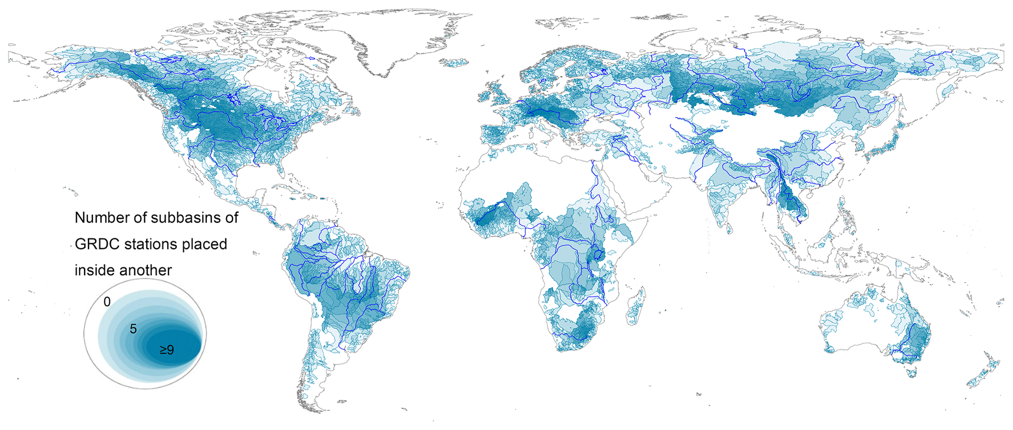
Figure 6 Watershed shapefile of 10 241 station using GRDC stations and MERIT network map (world administrative boundaries by https://www.opendatasoft.com, last access: 6 December 2023).

3.2 Station allocation at low resolution (5^′ and 30^′)

We allocated 10 241 stations with an area ≥10 km², and we created shapefiles and a station record for low resolutions of 30^′ and 5^′. For the resolution of 30^′, we used a threshold of a UPA of ≥9000 km² (around three grid cells at 30^′ resolution). For 5^′, we used a threshold of ≥1000 km² (∼12 grid cells at 5^′ resolution). This selection was subjective, and other papers have slightly different assumptions (Alfieri et al., 2020).

With the similarity method, we can avoid a basin being allocated to a station that fits better according to the UPA but is not very similar to the basin shapefile at high resolution. Figure 7 shows this for two examples. The Above Babine River station of the Skeena River in Canada, GRDC No. 4245920, is located shortly before the junction with the Babine River. If we take the location of the station GRDC No. 4245920 at 30^′ resolution, we obtain the Skeena and the Babine River joined together. We have to move the station to allocate it to the correct basin. The reported UPA of the station is 12 400 km². If we had selected only by upstream area or by weighted upstream area and distance, we would have chosen the Babine River (UPA of 30^′: 12 495 km²) over the Skeena River (UPA of 30^′: 11 937 km²). Figure 7a shows that the selected 30^′ basin in darker blue (Skeena River) with the lower UPA fits better with the high-resolution basin even if the distance to the cell center of the Skeena Basin is 59 km (distance between green dot and dark blue square) compared to the distance to the Babine River of 28 km (distance between green dot and red square).

Figure 7b shows a station mismatch selected by the UPA at 5^′. The Khudan River in Russia, GRDC No. 2907025, has a reported UPA of 7800 km². We only shifted the station by 0.8 km to fit the 3^′ high-resolution network. If we select by UPA, the Uda River, with a UPA at 5^′ resolution of 7901 km², fits better than the Khudan River, with a UPA at 5^′ resolution of 7673 km². Also, the cell center of the Uda River is closer to the station (4.4 km) than the cell center of the Khudan River (8.2 km). Selecting by area and shape similarity points to the correct basin, shown in dark blue in Fig. 7b.

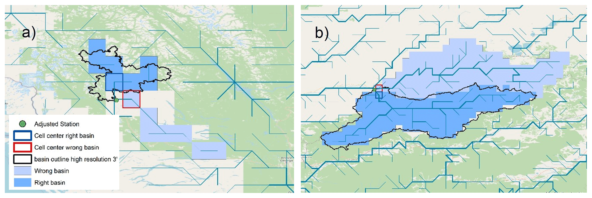
Figure 7 Mismatch of basin allocation because of selection from upstream area only. Panel (a) shows the Skeena River, Canada, at 30^′ resolution; (b) shows the Khudan River, Russia, at 5^′ resolution. © OpenStreetMap contributors 2022. Distributed under the Open Data Commons Open Database License (ODbL) v1.0.

For the coarser resolution of 5^′, we selected 6414 stations with a basin area ≥1000 km². For the resolution of 30', we selected 2741 stations with a basin area ≥9000 km². For the 2741 selected station resolution of 30^′, we found 68 cases (2 %) where the station location would account for the wrong basins, which the UPA and distance method could not detect. For 684 stations (25 %), we chose basin representations of the stations that fit better to similarity and UPA than to UPA and distance. For the 6414 selected stations for 5^′ resolution, we had 23 cases of station mismatch (0.7 %) and 680 (11 %) where we chose another basin representation than with UPA and distance. We assigned polygons based on the upscaled river network for those two resolutions. We provided the list of stations with adjusted station locations and the 5^′ and 30^′ watershed boundaries as shapefiles.

3.3 Selecting stations for calibration at low resolution (5^′ and 30^′)

Based on the selection criteria of Tables 1 and 2, we included meta information of the station time series (length and end date of the time series, number of missing values, daily or monthly values). As mentioned in Sect. 2, the selection criteria were subjective, but the Python code for changing the criteria tables is available on GitHub.

For the low resolution of 30^′, from the 2724 stations (with a UPA of ≥9000 km²), we selected 953 stations for calibration. Another 105 stations could be used for validation purposes. The latter stations are not in the first calibration category because they are equal to or more than 95 %, similar to a station chosen for calibration. We dismissed 1666 stations from the calibration because they do not fulfill the necessary criteria given in Table 1. For the low-resolution of 5^′, we selected 3917 out of 6415 stations. Another 175 stations were available for validation, and we dismissed 2323 stations.

Figure 8 and the histograms in Fig. 9 show the global distribution. North America, Brazil, Europe, Russia, and Australia are well covered but Asia and Africa only partly. At 5^′ resolution, 441 stations are in Africa, and 1270 and 746 are in North America and Europe.

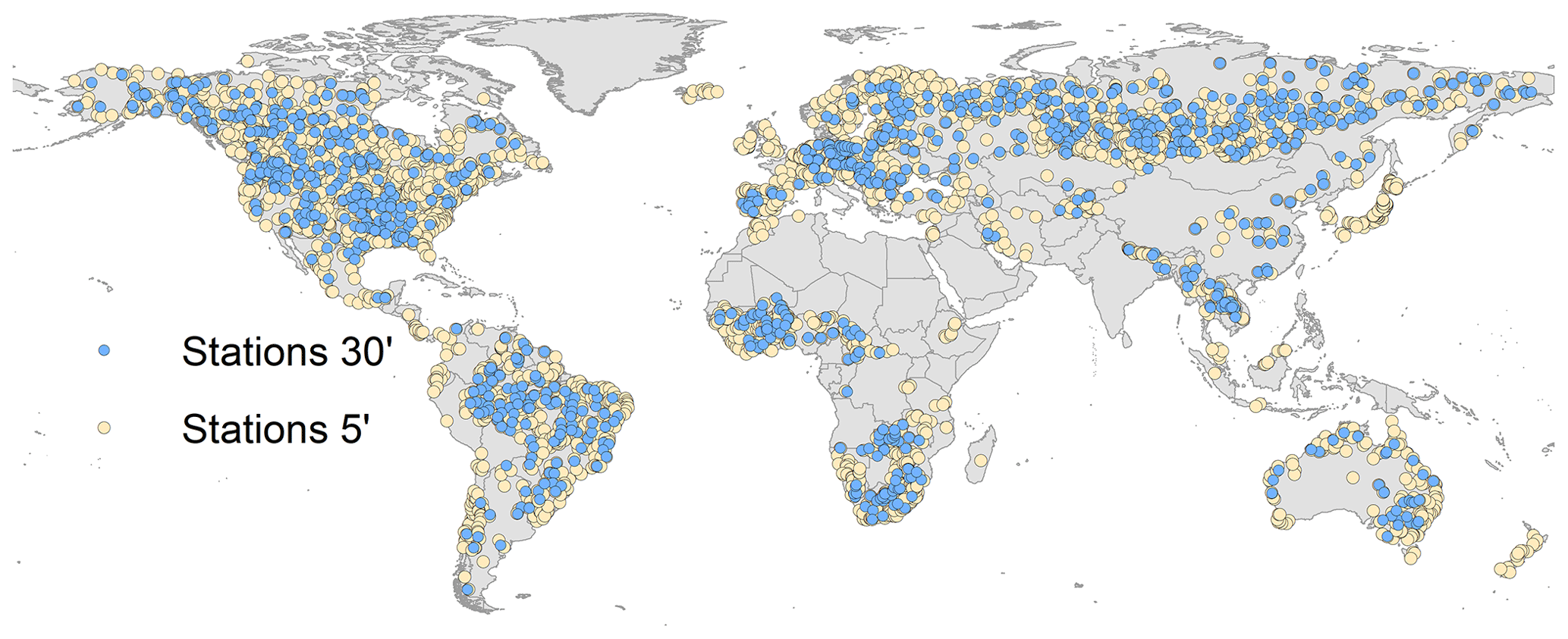
Figure 8 Selected station for calibration at 30^′ (949 stations) and 5^′ (3917 stations) resolution (world administrative boundaries by https://www.opendatasoft.com, last access: 6 December 2023).

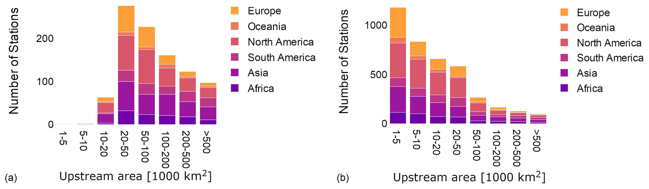
Figure 9 Histogram of selected calibration stations (a) 949 stations for 30^′; (b) 3917 stations for 5^′, classified by upstream area (shown in 1000 km²) and continent.

4 Code and data availability

The MERIT Hydro – global hydrography dataset is available for download at http://hydro.iis.u-tokyo.ac.jp/~yamadai/MERIT_Hydro (Yamazaki et al., 2019) and was last updated on 17 May 2019. The metadata information on 10 701 was provided by the Global Runoff Data Centre (GRDC, 2020, https://www.bafg.de/GRDC) (last access: 4 April 2022). The watershed boundaries based on Lehner et al. (2011) can be downloaded from GRDC.

The high-resolution (3^′′) and low-resolution (5^′ and 30^′) source code, tables, and shapefile datasets are stored on Zenodo with the associated DOI https://doi.org/10.5281/zenodo.6906577 (Burek and Smilovic, 2022). In addition, we provide the source code on a GitHub repository https://github.com/iiasa/CWATM_grdc_calibration_stations (last access: 6 December 2023) as release version 1.0. Here we used input data from MERIT Hydro with a resolution of 3^′′ and an eight-direction (D8) flow model network format, but the code can be changed to use any resolution and non-geographical projections as input format. Please keep in mind that the Zenodo repository is the location where users can retrieve the exact data that have been used in this study.

5 Conclusion

This paper describes the procedure used to generate a dataset of station locations of observed discharge to be used at different resolutions for calibrating large-scale hydrological models. It is based on the metadata of GRDC stations and MERIT Hydro. The Python source code and dataset produced are freely available for download through a GitHub and Zenodo repository.

The first step toward generating a high-resolution collection of watershed shapefiles was to update the work of Lehner (2012) to include more basins (10 241 stations vs. 7163) based on a higher-resolution river network database (3^′′ MERIT Hydro from Yamazaki et al. (2019) vs. 15^′′ the HydroSHEDS from Lehner et al. (2008), including the changed GRDC IDs from September 2021). The second step, generating a lower-resolution collection of watershed shapefiles based on the intersection-over-union ratio, was inspired by the ideas of Rezatofighi et al. (2019) and Munier and Decharme (2022). This is a better approach than selecting a station location from low-resolution river network systems based only on the UPA and distance to the original location. Here, we provide the low-resolution watershed boundaries at 30^′ and 5^′ resolution and the source code to produce results for different resolutions and projection systems. The third step, selecting suitable stations for calibration and validation, was also based on the intersection-over-union ratio. This selection of stations can now be used more effectively to calibrate grid-based hydrological models at different resolutions.

We are very grateful for the work of GRDC in collecting and making available a considerable number of stations. Around 8000 of the 10 701 stations fit very well and have less than a 5 % difference between the reported UPA and the MERIT Hydro-calculated UPA. Around 10 000 stations have less than 30 % UPA difference. For 228 stations, however, we could not find a suitable location, and for another 437 stations, the reported area and calculated area are very different (25 % error). Most stations (8544) could be located on the high-resolution MERIT network within a 1 km range. However, 843 stations have a corrected station location of more than 5 km distance from the original position. We propose a quality check for these stations; otherwise, the time series cannot be used for any applications.